chapter 1: review of stochastic process

Statistical Digital Signal Processing

Chapter 1: Introduction and Review of Stochastic Process

Objective of the Course

• To enable students analyze, represent andmanipulate random signals with LTI systems.– Understand challenges posed by random

signals,

– Understand how to model random signals,

– Understand how to represent random signals,

– Understand how to design LTI system toestimate random signals,

– Understand efficient algorithms to estimaterandom signals.

Bisrat Derebssa, SECE, AAiT, AAU

Content of the course

1. Introduction and Review of Stochastic Process

2. Linear Signal Modelling

3. Nonparametric Power Spectrum Estimation

4. Optimum Linear Estimation of Signals

5. Algorithms for Optimum Linear Filter

6. Adaptive Filters


References

• Statistical Digital Signal Processing andModeling, M. Hayes, Wiley, 1996.

• Statistical and Adaptive signal Processing,Dimitris G. Manolakis, Vinay K. Ingle,Stephen M. Kogon, Artech House, 2005

• Optimum Signal Processing, Sophocles J.Orfanidis, McGraw-Hill, 2007


Evaluation

• Assignment (20%)

• Mid Exam (30%)

• Final Exam (50%)


Random Variables

• Any random situation can be studied by theaxiomatic definitions of probability bydefining 𝑆, ℱ, 𝑃𝑟 .– 𝑆 = {𝜁1, 𝜁2, … } – Universal set of unpredictable

outcomes

– ℱ – collection of subset of 𝑆 whose elements are calledevents.

– Pr 𝜁𝑘, 𝑘 = 1,2, . . . – probability representing the

unpredictability of these events.


• Difficult to work with this probability spacefor two reasons.–The basic space contains abstract events and

outcomes that are difficult to manipulate.• We want random outcomes that can be measured and

manipulated in a meaningful way by using numericaloperations.

–The probability function Pr {·} is a set functionthat again is difficult, to manipulate by usingcalculus.


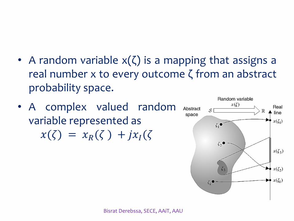
• A random variable x(ζ) is a mapping that assigns areal number x to every outcome ζ from an abstractprobability space.

• A complex valued randomvariable represented as𝑥(𝜁) = 𝑥𝑅(𝜁 ) + 𝑗𝑥𝐼(𝜁


•This mapping should satisfy the following twoconditions:–the interval {X(ζ) ≤ x } is an event in the abstract

probability space for every x ;

–Pr {X(ζ) =∞}=0 and Pr{X(ζ) = −∞} =0.

• A random variable is called discrete-valued ifx takes a discrete set of values {xk};

• Otherwise, it is termed a continuous-valuedrandom variable.


Representation of Random VariablesCumulative distribution function (CDF)

𝐹𝑋 𝑥 = 𝑃𝑟{𝑋(𝜁) ≤ 𝑥}

Probability density function (pdf ) 𝑓𝑋 𝑥 =

𝑑𝐹𝑋 𝑥

𝑑𝑥

Expectation of a random variable

𝐸 𝑥 𝜁 = 𝜇𝑥 =

𝑥

𝑥𝑘𝑝𝑥

න−∞

∞

𝑥𝑓𝑋 𝑥 𝑑𝑥

Expectation of a functionof random variable

𝐸 𝑔 𝑥 𝜁 = න−∞

∞

𝑔(𝑥)𝑓𝑋 𝑥 𝑑𝑥

Moments 𝑟𝑥(𝑚)

= 𝐸 𝑥𝑚 𝜁 = න−∞

∞

𝑥𝑚𝑓𝑋 𝑥 𝑑𝑥

Central Moments𝛾𝑥(𝑚)

= 𝐸 𝑥 𝜁 − 𝜇𝑥𝑚 = න

−∞

∞

𝑥 − 𝜇𝑥𝑚𝑓𝑋 𝑥 𝑑𝑥


Second central moment or variance 𝜎𝑥

2 = 𝛾𝑥(2)

= 𝐸 𝑥 𝜁 − 𝜇𝑥2

Skewness 𝑘𝑥(3)

=1

𝜎𝑥3 𝛾𝑥

(3)

Kurtosis 𝑘𝑥~(4)

=1

𝜎𝑥4 𝛾𝑥

(4)− 3

Characteristic functions 𝚽𝑥 𝜉 = 𝐸 𝑒𝑗𝜉𝑥 𝜁 = න−∞

∞

𝑓𝑋 𝑥 𝑒𝑗𝜉𝑥𝑑𝑥

Moment generating functionsഥ𝚽𝒙 𝑠 = 𝐸 𝑒𝑠𝑥 𝜁 = න

−∞

∞

𝑓𝑋 𝑥 𝑒𝑠𝑥𝑑𝑥

Cumulants generating functions ഥ𝚿𝑥 𝑠 = ln ഥ𝚽𝑥 𝑠 = ln 𝐸 𝑒𝑠𝑥 𝜁

Cumulants 𝑘𝑥(𝑚)

= อd𝑚[ഥ𝚿𝑥 𝑠 ]

d𝑠𝑚𝑠=0


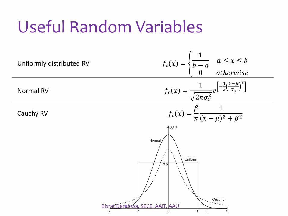
Useful Random Variables

Uniformly distributed RV 𝑓𝑥 𝑥 = ቐ1

𝑏 − 𝑎𝑎 ≤ 𝑥 ≤ 𝑏

0 𝑜𝑡ℎ𝑒𝑟𝑤𝑖𝑠𝑒

Normal RV 𝑓𝑥 𝑥 =1

2𝜋𝜎𝑥2𝑒−12𝑥−𝜇𝜎𝑥

2

Cauchy RV 𝑓𝑥 𝑥 =𝛽

𝜋

1

𝑥 − 𝜇 2 + 𝛽2


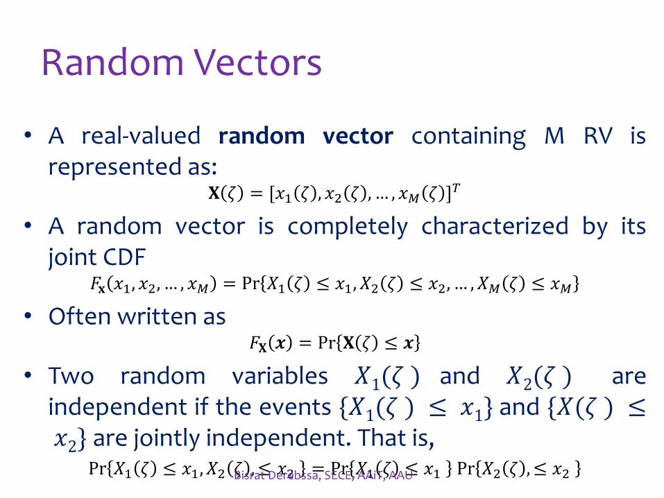
Random Vectors

• A real-valued random vector containing M RV isrepresented as:

𝐗 𝜁 = [𝑥1 𝜁 , 𝑥2 𝜁 , … , 𝑥𝑀 𝜁 ]𝑇

• A random vector is completely characterized by itsjoint CDF

𝐹𝐱 𝑥1, 𝑥2, … , 𝑥𝑀 = Pr 𝑋1 𝜁 ≤ 𝑥1, 𝑋2 𝜁 ≤ 𝑥2, … , 𝑋𝑀 𝜁 ≤ 𝑥𝑀

• Often written as𝐹𝐗 𝒙 = Pr 𝐗 𝜁 ≤ 𝒙

• Two random variables 𝑋1(𝜁 ) and 𝑋2(𝜁 ) areindependent if the events {𝑋1(𝜁 ) ≤ 𝑥1} and {𝑋(𝜁 ) ≤𝑥2} are jointly independent. That is,

Pr 𝑋1 𝜁 ≤ 𝑥1, 𝑋2 𝜁 ,≤ 𝑥2 = Pr 𝑋1 𝜁 ≤ 𝑥1 Pr 𝑋2 𝜁 , ≤ 𝑥2Bisrat Derebssa, SECE, AAiT, AAU

• The probability functions require anenormous amount of information that is noteasy to obtain or is too complexmathematically for practical use.

• In practical applications, random vectors aredescribed by less complete but moremanageable statistical averages.


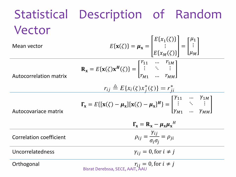
Statistical Description of RandomVector

Mean vector 𝐸 𝐱 𝜁 = 𝝁𝐱 =𝐸 𝑥1 𝜁

⋮𝐸 𝑥𝑀 𝜁

=

𝜇1⋮𝜇𝑀

Autocorrelation matrix𝐑𝐱 = 𝐸 𝐱 𝜁 𝐱𝑯 𝜁 =

𝑟11 … 𝑟1𝑀⋮ ⋱ ⋮𝑟𝑀1 … 𝑟𝑀𝑀

Autocovariace matrix𝚪𝐱 = 𝐸 𝐱 𝜁 − 𝝁𝐱 𝐱 𝜁 − 𝝁𝐱

𝑯 =

𝛾11 … 𝛾1𝑀⋮ ⋱ ⋮

𝛾𝑀1 … 𝛾𝑀𝑀

𝚪𝐱 = 𝐑𝐱 − 𝝁𝐱𝝁𝐱𝐻

Correlation coefficient 𝜌𝑖𝑗 =𝛾𝑖𝑗

𝜎𝑖𝜎𝑗= 𝜌𝑗𝑖

Uncorrelatedness 𝛾𝑖𝑗 = 0, for 𝑖 ≠ 𝑗

Orthogonal 𝑟𝑖𝑗 = 0, for 𝑖 ≠ 𝑗Bisrat Derebssa, SECE, AAiT, AAU

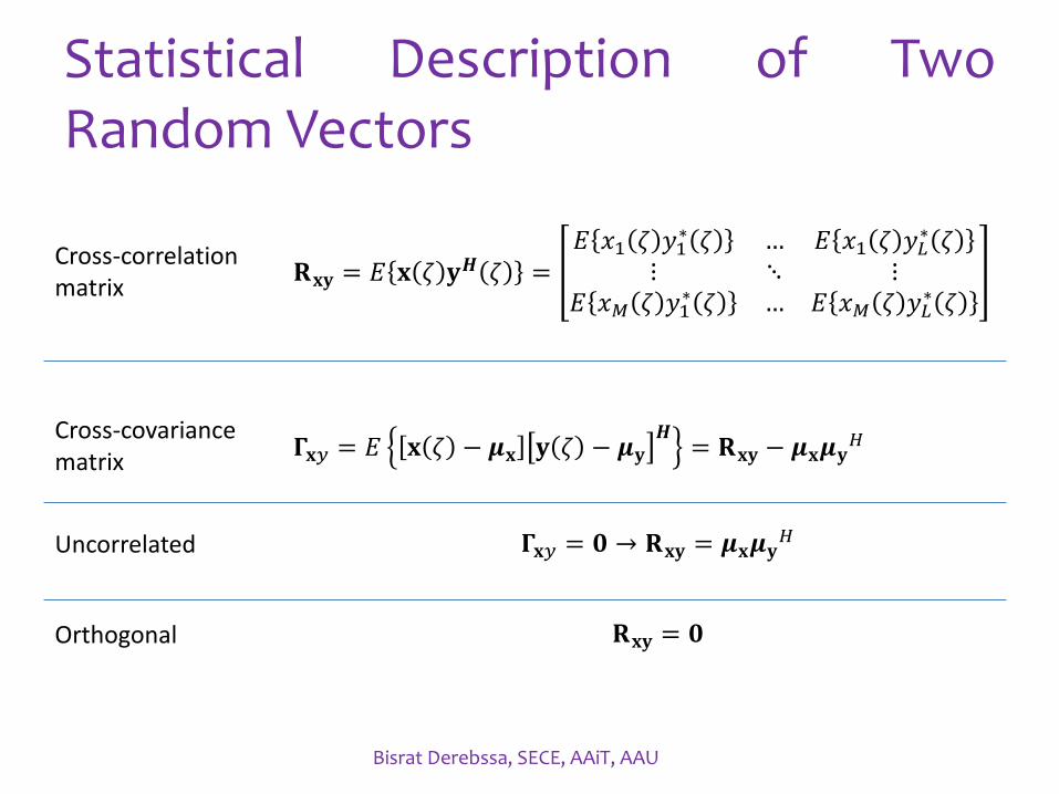
Statistical Description of TwoRandom Vectors

Cross-correlation matrix

𝐑𝐱𝐲 = 𝐸 𝐱 𝜁 𝐲𝑯 𝜁 =𝐸 𝑥1 𝜁 𝑦1

∗ 𝜁 … 𝐸 𝑥1 𝜁 𝑦𝐿∗ 𝜁

⋮ ⋱ ⋮𝐸 𝑥𝑀 𝜁 𝑦1

∗ 𝜁 … 𝐸 𝑥𝑀 𝜁 𝑦𝐿∗ 𝜁

Cross-covariance matrix

𝚪𝐱𝑦 = 𝐸 𝐱 𝜁 − 𝝁𝐱 𝐲 𝜁 − 𝝁𝐲𝑯

= 𝐑𝐱𝐲 − 𝝁𝐱𝝁𝐲𝐻

Uncorrelated 𝚪𝐱𝑦 = 𝟎 → 𝐑𝐱𝐲 = 𝝁𝐱𝝁𝐲𝐻

Orthogonal 𝐑𝐱𝐲 = 𝟎


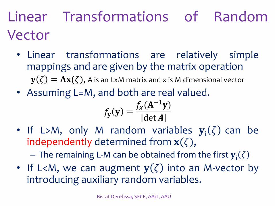
Linear Transformations of RandomVector• Linear transformations are relatively simple

mappings and are given by the matrix operation𝐲 𝜁 = 𝐀𝐱(𝜁), A is an LxM matrix and x is M dimensional vector

• Assuming L=M, and both are real valued.

𝑓𝐲 𝐲 =𝑓𝑥(𝐀

−1𝐲)

det 𝑨

• If L>M, only M random variables 𝐲𝐢 𝜁 can beindependently determined from 𝐱(𝜁),– The remaining L-M can be obtained from the first 𝐲𝐢 𝜁

• If L<M, we can augment 𝐲 𝜁 into an M-vector byintroducing auxiliary random variables.


• For complex valued RV,

𝑓𝐲 𝐲 =𝑓𝑥(𝐀

−1𝐲)

det 𝑨 2

• The determination of 𝑓𝐲 𝐲 is tedious and in

practice not necessary.


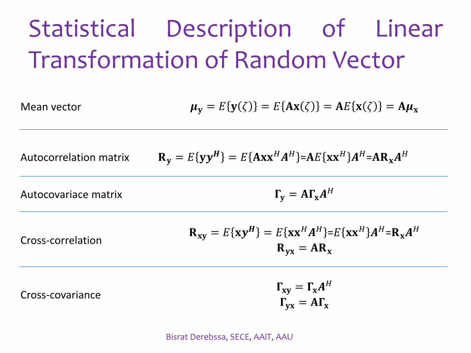
Statistical Description of LinearTransformation of Random Vector

Mean vector 𝝁𝐲 = 𝐸 𝐲 𝜁 = 𝐸 𝐀𝐱 𝜁 = 𝐀𝐸 𝐱 𝜁 = 𝐀𝝁𝐱

Autocorrelation matrix 𝐑𝐲 = 𝐸 𝐲𝒚𝑯 = 𝐸 𝐀𝐱𝐱𝐻𝑨𝐻 =𝐀𝐸 𝐱𝐱𝐻 𝑨𝐻=𝐀𝐑𝐱𝑨𝐻

Autocovariace matrix 𝚪𝐲 = 𝐀𝚪𝐱𝑨𝐻

Cross-correlation𝐑𝐱𝐲 = 𝐸 𝐱𝒚𝑯 = 𝐸 𝐱𝐱𝐻𝑨𝐻 =𝐸 𝐱𝐱𝐻 𝑨𝐻=𝐑𝐱𝑨

𝐻

𝐑𝐲𝐱 = 𝐀𝐑𝐱

Cross-covariance𝚪𝐱𝐲 = 𝚪𝐱𝑨

𝐻

𝚪𝐲𝐱 = 𝐀𝚪𝐱


Normal Random Vectors

• If the components of the random vector x (ζ ) arejointly normal, then x (ζ ) is a normal random M -vector.

• For real valued normal random vector

𝑓𝐱 𝐱 =1

(2𝜋) ൗ𝑀 2 𝚪𝐱ൗ1 2𝑒−12𝐱−𝛍𝐱

𝑇𝚪𝐱−1 𝐱−𝛍𝐱

• Its characteristic equation is

Φ𝐱(𝝃) = 𝑒𝑗𝝃𝑇𝝁𝐱−

12𝝃𝑇𝚪𝐱𝝃


Properties of normal random vector

• Pdf and all higher order momentscompletely specified from mean vector andcovariance matrix.

• If the components of 𝐱 𝜁 are mutuallyuncorrelated, they are also independent.

• A linear transformation of a normal randomvector is also normal.


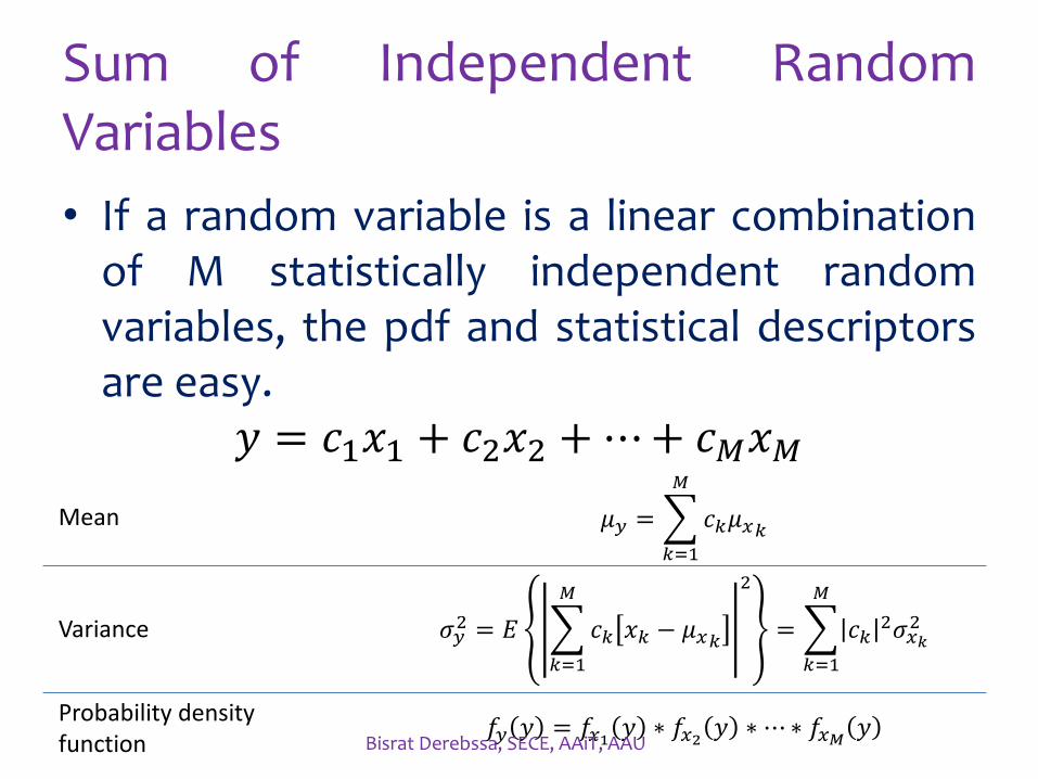
Sum of Independent RandomVariables

• If a random variable is a linear combinationof M statistically independent randomvariables, the pdf and statistical descriptorsare easy.

𝑦 = 𝑐1𝑥1 + 𝑐2𝑥2 +⋯+ 𝑐𝑀𝑥𝑀

Mean 𝜇𝑦 =

𝑘=1

𝑀

𝑐𝑘𝜇𝑥𝑘

Variance 𝜎𝑦2 = 𝐸

𝑘=1

𝑀

𝑐𝑘 𝑥𝑘 − 𝜇𝑥𝑘

2

=

𝑘=1

𝑀

𝑐𝑘2𝜎𝑥𝑘

2

Probability density function

𝑓𝑦 𝑦 = 𝑓𝑥1 𝑦 ∗ 𝑓𝑥2 𝑦 ∗ ⋯∗ 𝑓𝑥𝑀 𝑦Bisrat Derebssa, SECE, AAiT, AAU

• Example: What is the pdf of y if its is the sum offour identical independent random variablesuniformly distributed over [-0.5, 0.5].

• Solution:U[-0.5, 0.5]*U[-0.5, 0.5]= fx12 fx12*U[-0.5, 0.5]=fx123 fx123*U[-0.5, 0.5]=fx1234


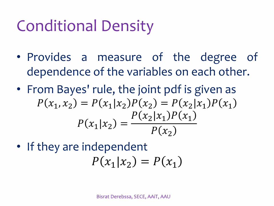
Conditional Density

• Provides a measure of the degree ofdependence of the variables on each other.

• From Bayes' rule, the joint pdf is given as𝑃 𝑥1, 𝑥2 = 𝑃 𝑥1|𝑥2 𝑃 𝑥2 = 𝑃 𝑥2|𝑥1 𝑃 𝑥1

𝑃 𝑥1|𝑥2 =𝑃 𝑥2|𝑥1 𝑃 𝑥1

𝑃 𝑥2

• If they are independent𝑃 𝑥1|𝑥2 = 𝑃 𝑥1


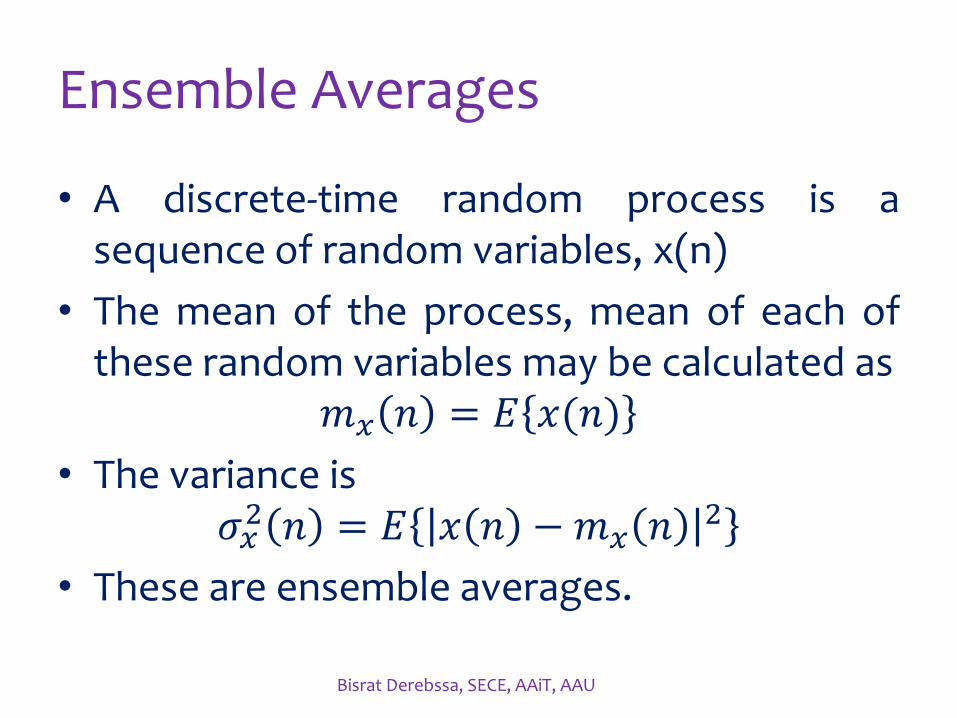
Ensemble Averages

• A discrete-time random process is asequence of random variables, x(n)

• The mean of the process, mean of each ofthese random variables may be calculated as

𝑚𝑥 𝑛 = 𝐸 𝑥(𝑛)

• The variance is𝜎𝑥2 𝑛 = 𝐸 𝑥 𝑛 −𝑚𝑥 𝑛 2

• These are ensemble averages.


• The autocorrelation of the process is𝑟𝑥 𝑘, 𝑙 = 𝐸 𝑥 𝑘 𝑥∗(𝑙)

• This provides the statistical relationshipbetween the random variables x(k) and x(l).

• Wide-sense stationary

– Mean of process is constant,

– Autocorrelation dependent only on (k-l)

– Variance is finite


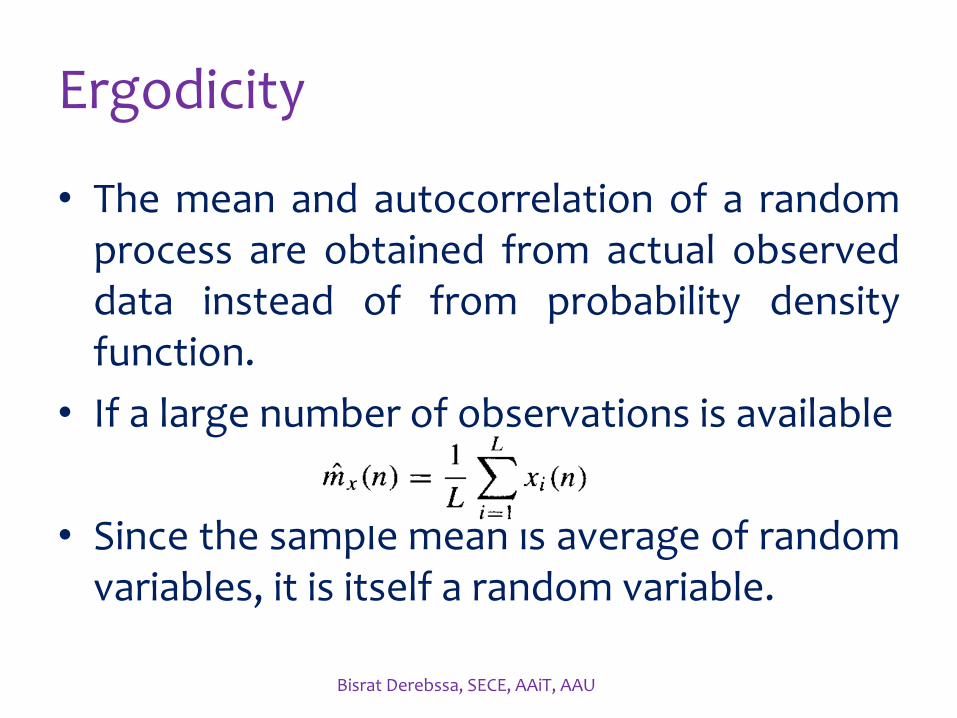
Ergodicity

• The mean and autocorrelation of a randomprocess are obtained from actual observeddata instead of from probability densityfunction.

• If a large number of observations is available

• Since the sample mean is average of randomvariables, it is itself a random variable.


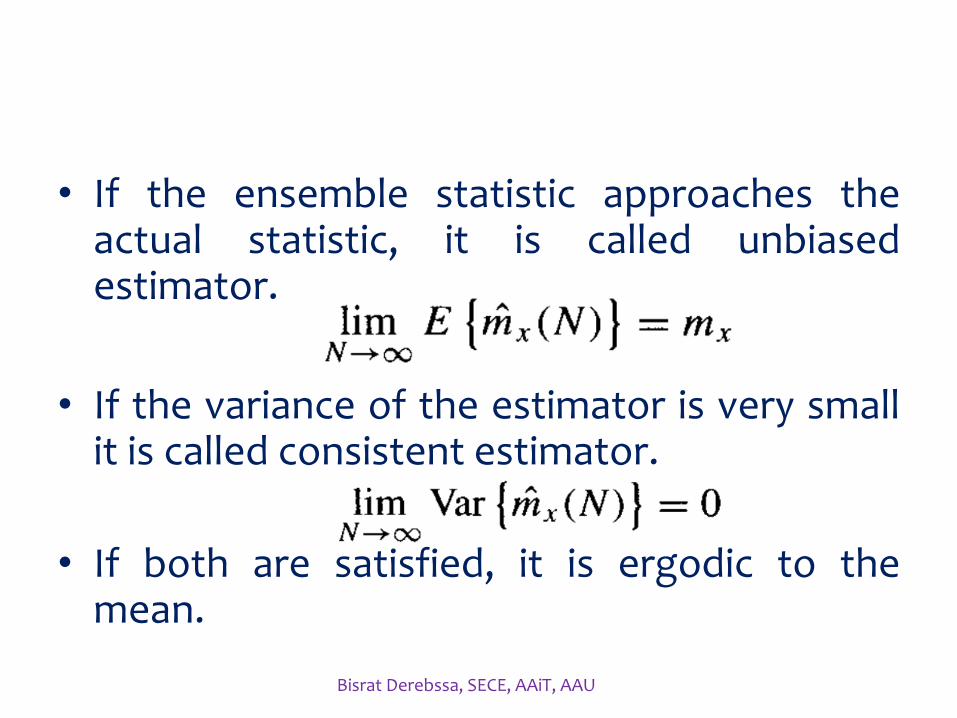
• If the ensemble statistic approaches theactual statistic, it is called unbiasedestimator.

• If the variance of the estimator is very smallit is called consistent estimator.

• If both are satisfied, it is ergodic to themean.


• This ergodicity principle may be generalizedto other ensemble averages.


Random Processes through LinearTime-invariant Systems

• Consider a linear time-invariant system withimpulse response h(t) driven by a randomprocess input X(t)


• It is difficult to obtain a completespecification of the output process ingeneral,

– The input is known only probabilistically.

• The mean and autocorrelation of the outputcan be determined in terms of the mean andautocorrelation of the input.


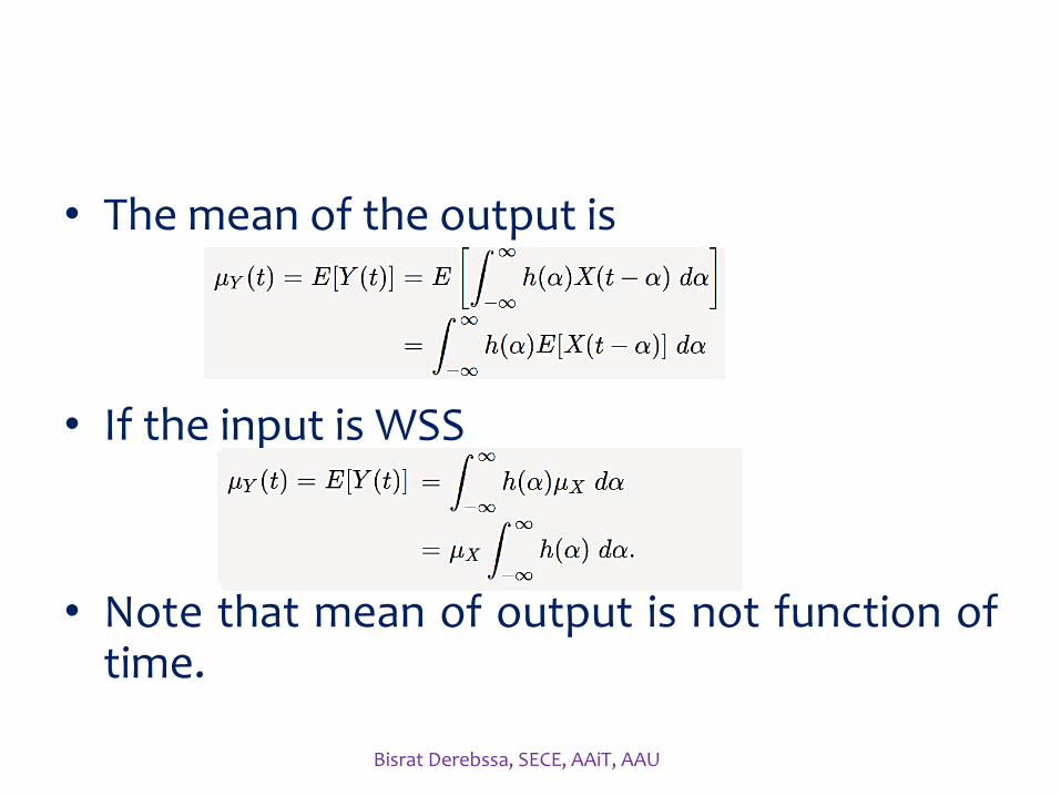
• The mean of the output is

• If the input is WSS

• Note that mean of output is not function oftime.


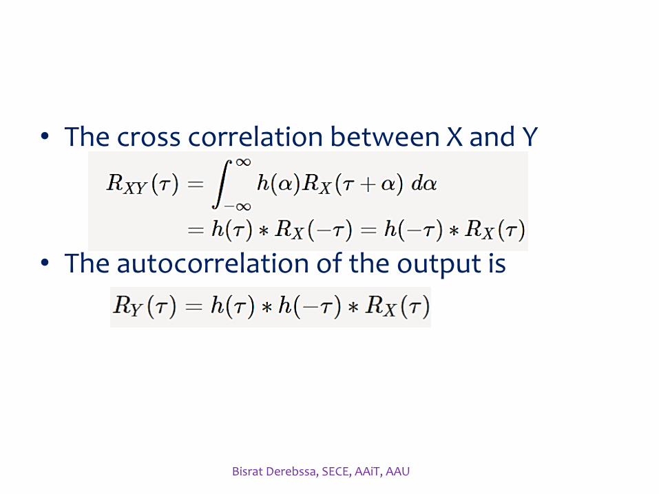
• The cross correlation between X and Y

• The autocorrelation of the output is


Power Spectrum

• The Fourier transform is important in therepresentation of random processes.

• Since random signals are only knownprobabilistically, it is not possible tocompute the Fourier transform directly.

• For a wide-sense stationary random process,the autocorrelation is a deterministicfunction of time.


• The periodogram is an estimation of thepower spectrum

• The autocorrelation sequence can beobtained from the periodogram


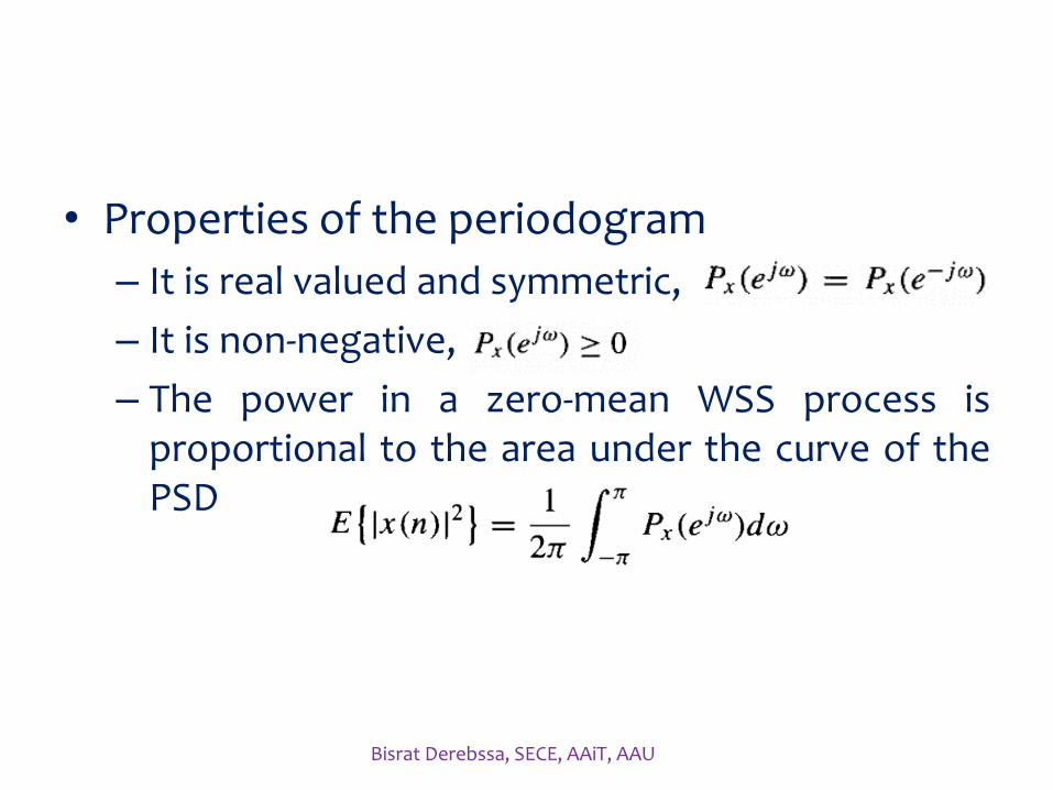
• Properties of the periodogram

– It is real valued and symmetric,

– It is non-negative,

– The power in a zero-mean WSS process isproportional to the area under the curve of thePSD


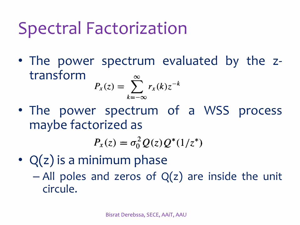
Spectral Factorization

• The power spectrum evaluated by the z-transform

• The power spectrum of a WSS processmaybe factorized as

• Q(z) is a minimum phase– All poles and zeros of Q(z) are inside the unit

circule.


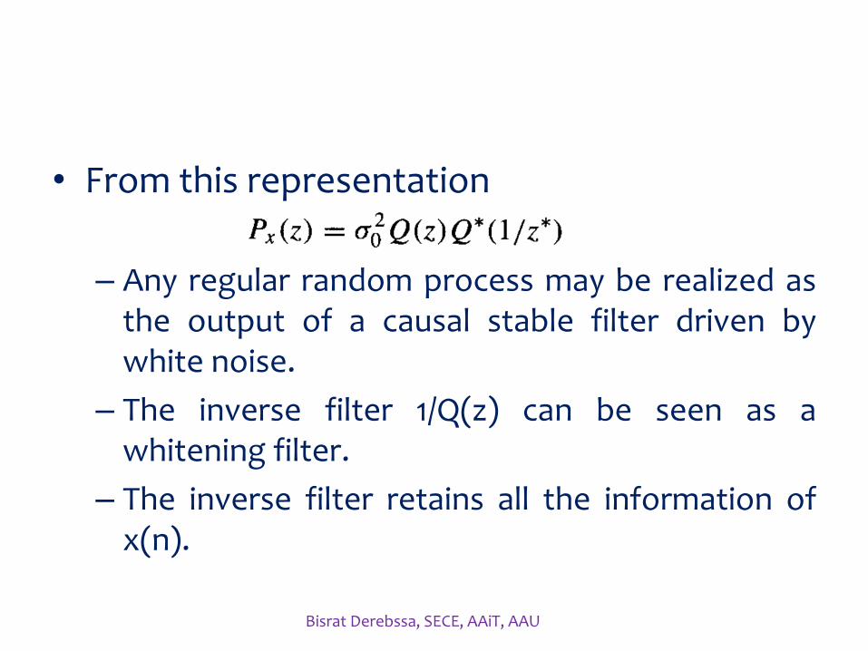
• From this representation

– Any regular random process may be realized asthe output of a causal stable filter driven bywhite noise.

– The inverse filter 1/Q(z) can be seen as awhitening filter.

– The inverse filter retains all the information ofx(n).


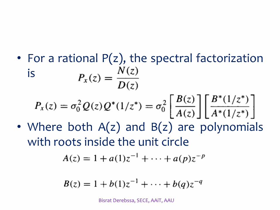
• For a rational P(z), the spectral factorizationis

• Where both A(z) and B(z) are polynomialswith roots inside the unit circle


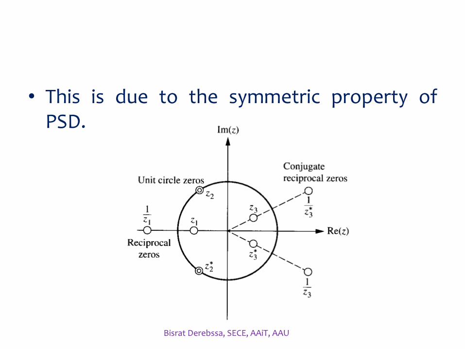
• This is due to the symmetric property ofPSD.


Assignment 1

• 1.1 Show that if the mth derivative of the momentgenerating function with respect to 𝑠 evaluated at 𝑠 =0results in the mth moment.

• 1.2 Find the mean, variance, moments and momentgenerating functions of Uniform, Normal and Cauchy RV.

• 1.3 Show that a linear transformation of a normal randomvector is also normal.

• 1.4 Find the spectral factorization of the following function.


• 1.5 The input to a linear shift-invariant filter with unit sampleresponse h(n) is a zero-mean wide-sense stationaryprocesses with autocorrelation rx(k). Find theautocorrelation of the output processes for all k and itsvariance.

ℎ 𝑛 = 𝛿 𝑛 −1

3𝛿 𝑛 − 1 +

1

4𝛿 𝑛 − 2

𝑟𝑥 𝑘 =1

2

|𝑘|


chapter 1: review of stochastic process

Documents