chapter 1sethi/postscript/lost sales template.pdfchapter 1 average cost optimality in inventory...

Chapter 1

AVERAGE COST OPTIMALITY ININVENTORY MODELS WITH MARKO-VIAN DEMANDS AND LOST SALES∗

Dirk BeyerHewlett-Packard [email protected]

Suresh P. SethiUniversity of Texas at DallasCorresponding [email protected]

Abstract This paper is concerned with long-run average cost minimization of astochastic inventory problem with Markovian demand, fixed orderingcost, convex surplus cost, and lost sales. The states of the Markovchain represent different possible states of the environment. Using avanishing discount approach, a dynamic programming equation and thecorresponding verification theorem are established. Finally, the exis-tence of an optimal state-dependent (s, S) policy is proved.

1. IntroductionIn the literature of stochastic inventory models, there are two different

assumptions about the excess demand unfilled from existing inventories:the backlog assumption and the lost sales assumption. The former ismore popular in the literature partly because historically the inventorystudies started with spare parts inventory management problems in mil-itary applications, where the backlog assumption is realistic. However,

∗This research was supported in part by NSERC grant A4619 and a grant from The Universityof Texas at Dallas.

2

in many other business situations, it is quite often that demand thatcannot be satisfied on time is lost. This is particularly true in a compet-itive business environment. For example in many retail establishments,such as a supermarket or a department store, a customer chooses a com-petitive brand or goes to another store if his/her preferred brand is outof stock.

In the presence of fixed ordering costs in inventory models under eitherassumption, an important issue has been to establish the optimality of(s, S)-type policies. There are many classical and recent papers thatdeal with this issue in the backlog case. These are cited and reviewedin Beyer and Sethi (1997,1999); see also the forthcoming book of Beyer,Cheng and Sethi (2004). However, only Veinott (1966), Shreve (1976),Bensoussan, Crouhy and Proth (1983), and Cheng and Sethi (1999),to our knowledge, have considered the lost sales case explicitly. Thisis perhaps because the proofs of the results in the lost sales case areusually more complicated than those in the backlog case. Shreve (1976)and Bensoussan, Crouhy and Proth (1983) establish the optimality of an(s, S)-type policy by using the concept of K-convexity. Veinott (1966)provides a different proof for the optimality of (s, S)-type policies inthe lost sales case. His proof is based on a different set of assumptionswhich neither implies nor is implied by those used in Shreve (1976) andBensoussan, Crouhy and Proth (1983). It should be noted that all theseresults are obtained under the condition of zero lead time. Cheng andSethi (1999) is discussed below.

Many efforts have been made to incorporate various realistic featuresin inventory models. However, most of them are carried out under thebacklog assumption. One such feature is that of Markovian demand,which has been considered by Karlin and Fabens (1960), Song and Zip-kin (1993), Sethi and Cheng (1997), Ozekici and Parlar (1999), Beyerand Sethi (1997,1999), and Beyer, Sethi and Taksar (1998). Withoutexception, they all use the backlog assumption in their analysis. As anatural extension of and a flexible alternative to independent demandsconsidered in the bulk of the classical inventory literature, Markoviandemands can model demands that are dependent on randomly chang-ing economic and market conditions. As the lost sales situation is oftenthe case in competitive markets, it is interesting and worthwhile to ex-tend the Markovian demand model to incorporate the lost sales case.Cheng and Sethi (1999) accomplish this in the discounted cost case. Itis the purpose of this paper to treat that lost sales case with Markoviandemands from the viewpoint of minimizing long-run average cost.

The plan of the paper is as follows. In the next section, we provide aprecise formulation of the problem. Relevant results for the discounted

Average Cost Optimality in Inventory Models 3

cost problem obtained in Cheng and Sethi (1999) are summarized inSection 1.3. Also examined in this section is the asymptotic behavior ofthe differential discounted value function as the discount rate approacheszero. In Section 1.4, we develop the vanishing discount approach to es-tablish the average cost optimality equation. The associated verificationtheorem is proved in Section 1.5, and the theorem is used to show thata state-dependent (s, S) policy, or simply an (si, Si) policy, is optimalfor the problem. Section 1.6 concludes the paper with suggestions forfuture research.

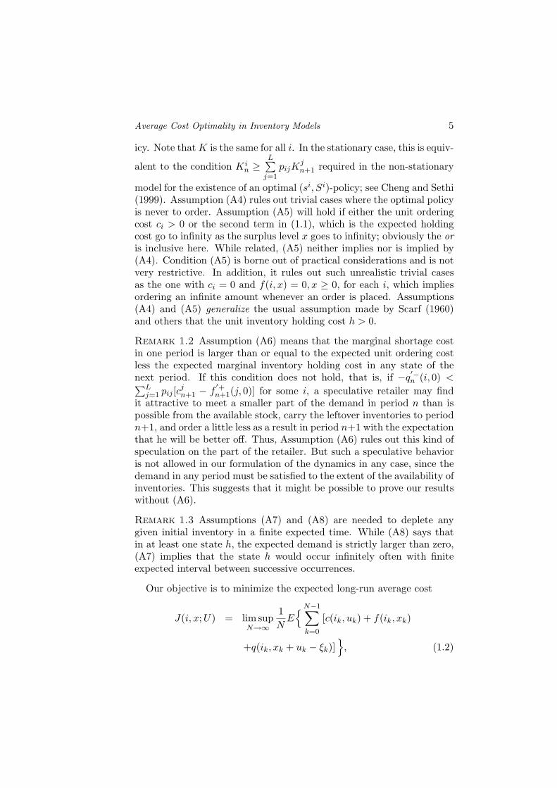
2. Formulation of the ModelIn order to specify the stationary, discrete time, infinite horizon inven-

tory problem under consideration, we introduce the following notationand basic assumptions:

(Ω,F , P ) = the probability space;I = 1, 2, . . . , L, a finite collection of possible demand

states;ik = the demand state in period k, k ∈ Z = 0, 1, 2, . . . ;

ik = a Markov chain with the (L× L)-transition matrixP = pij;

ξk = the demand realized during the period k, ξk

dependent on ik, but not on k;φi(·) = the conditional density function of ξk when ik = i;Φi(·) = the distribution function corresponding to φi;

uk = the nonnegative order quantity in period k;xk = the (non-negative) inventory level at the beginning

of period k (or, at the end of period k − 1);c(i, u) = the cost of ordering u ≥ 0 units in period k when

ik = i;f(i, x) = the inventory cost when ik = i and xk = x ≥ 0;

q(i, x + u− ξ) = the shortage cost when ik = i, xk = x, uk = u, andξk = ξ;

δ(z) = 0, 1, respectively, when z ≤ 0, z > 0, respectively.

We suppose that orders are placed at the beginning of a period, de-livered instantaneously, and followed by the period’s demand; see Fig-ure 1.1. Unsatisfied demands are lost.

4

0 1 2 k k + 1 k + 2

period 0 period 1 period k period k + 1

?

6ξk

?

6

uk

?

6

yk

?

6

xk ?

6xk+1

Figure 1.1. Temporal conventions used for the discrete-time inventory problem.

We make the following assumptions throughout the paper. While notall the results proved in this paper require all of the assumptions, wedo use all of the assumptions to derive the main results of the paperin Sections 1.4 and 1.5. For specificity, we shall list the assumptionsrequired in the statements of the results proved in this paper.Assumption A1. The production cost is given by c(i, u) = Kδ(u)+ciu,where the fixed ordering cost K ≥ 0 and the variable cost ci ≥ 0.Assumption A2. For each i, the inventory cost function f(i, ·) is con-vex, non-decreasing and of linear growth, i.e., f(i, x) ≤ Cf (1 + |x|) forsome Cf > 0 and all x. Also f(i, x) = 0 for all x ≤ 0.Assumption A3. For each i, the shortage cost function q(i, ·) is convex,non-increasing and of linear growth, i.e., q(i, x) ≤ Cq(1 + |x|) for someCq > 0 and all x. Also q(i, x) = 0 for all x ≥ 0.Assumption A4. There is a state g ∈ I such that f(g, x) is not iden-tically zero.Assumption A5. The production and inventory costs satisfy for all i,

cix +L∑

j=1

pij

∞∫

0

f(j, (x− z)+)ϕi(z)dz →∞ as x →∞. (1.1)

Assumption A6. For each i, q′−(i, 0) ≤ ∑L

j=1 pij(f′+(j, 0)−cj), where

the supersripts ‘+’ and ‘−’ denote the right-hand and left-hand deriva-tives.Assumption A7. The Markov chain (ik)∞k=0 is irreducible.Assumption A8. There is a state h ∈ I such that 1 − Φh(ε) = ρ > 0for some ε > 0.Assumption A9. E(ξi) < ∞ for each i.

Remark 1.1 Assumptions (A1)–(A3) reflect the usual structure of theproduction and inventory costs to prove the optimality of an (si, Si) pol-


icy. Note that K is the same for all i. In the stationary case, this is equiv-

alent to the condition Kin ≥

L∑j=1

pijKjn+1 required in the non-stationary

model for the existence of an optimal (si, Si)-policy; see Cheng and Sethi(1999). Assumption (A4) rules out trivial cases where the optimal policyis never to order. Assumption (A5) will hold if either the unit orderingcost ci > 0 or the second term in (1.1), which is the expected holdingcost go to infinity as the surplus level x goes to infinity; obviously the oris inclusive here. While related, (A5) neither implies nor is implied by(A4). Condition (A5) is borne out of practical considerations and is notvery restrictive. In addition, it rules out such unrealistic trivial casesas the one with ci = 0 and f(i, x) = 0, x ≥ 0, for each i, which impliesordering an infinite amount whenever an order is placed. Assumptions(A4) and (A5) generalize the usual assumption made by Scarf (1960)and others that the unit inventory holding cost h > 0.

Remark 1.2 Assumption (A6) means that the marginal shortage costin one period is larger than or equal to the expected unit ordering costless the expected marginal inventory holding cost in any state of thenext period. If this condition does not hold, that is, if −q

′−n (i, 0) <∑L

j=1 pij [cjn+1 − f

′+n+1(j, 0)] for some i, a speculative retailer may find

it attractive to meet a smaller part of the demand in period n than ispossible from the available stock, carry the leftover inventories to periodn+1, and order a little less as a result in period n+1 with the expectationthat he will be better off. Thus, Assumption (A6) rules out this kind ofspeculation on the part of the retailer. But such a speculative behavioris not allowed in our formulation of the dynamics in any case, since thedemand in any period must be satisfied to the extent of the availability ofinventories. This suggests that it might be possible to prove our resultswithout (A6).

Remark 1.3 Assumptions (A7) and (A8) are needed to deplete anygiven initial inventory in a finite expected time. While (A8) says thatin at least one state h, the expected demand is strictly larger than zero,(A7) implies that the state h would occur infinitely often with finiteexpected interval between successive occurrences.

Our objective is to minimize the expected long-run average cost

J(i, x;U) = lim supN→∞

1N

E N−1∑

k=0

[c(ik, uk) + f(ik, xk)

+q(ik, xk + uk − ξk)]

, (1.2)

6

with i0 = i and x0 = x ≥ 0, where U = (u0, u1, . . .), ui ≥ 0, i = 0, 1, . . . ,is a history-dependent or non-anticipative decision (order quantities) forthe problem. Such a control U is termed admissible. Let U denote theclass of all admissible controls. The surplus balance equations are givenby

xk+1 = (xk + uk − ξk+1)+, k = 0, 1, . . . . (1.3)

Our aim is to show that (i) there exists a constant λ∗ termed the optimalaverage cost, which is independent of the initial i and x, (ii) a controlU∗ ∈ U such that

λ∗ = J(i, x; U∗) ≤ J(i, x; U), for all U ∈ U , (1.4)

and (iii)

λ∗ = limN→∞

1N

E

N−1∑

k=0

[c(ik, u∗k) + f(ik, x∗k) + q(ik, xk + uk − ξk)]

,

(1.5)where x∗k, k = 0, 1, . . . , is the surplus process corresponding to U∗ withi0 = i and x0 = x.

To prove these results we will use the vanishing discount approach.That is, by letting the discount factor α in the discounted cost problemapproach 1, we will show that we can derive a dynamic programmingequation whose solution provides an average optimal control and theassociated minimum average cost λ∗.

For this purpose, we recapitulate relevant results for the discountedcost problem obtained in Cheng and Sethi (1999).

Remark 1.4 It may be noted that the objective function (1.2) is slightly,but not essentially, different from that used in the classical literature.Whereas we base the surplus cost on the initial surplus in each period,the usual practice in the literature is to charge the cost on the endingsurplus levels, which means to have f(ik, xk+1) instead f(ik, xk) in (1.2).Note that the xk+1 is also the ending inventory in period k. It should beobvious that this difference in the objective functions does not changethe long-run average cost for any admissible policy. By the same tokenwe can justify our choice to charge shortage cost at the end of a givenperiod.


3. Markovian Demand Model With DiscountedCosts

Consider the model formulated above with the average cost objective(1.2) replaced by the following extended real-valued objective function:

Jα(i, x; U) =∞∑

k=0

αkE[c(ik, uk)+f(ik, xk)+q(ik, xk+uk−ξk)], 0 ≤ α < 1.

(1.6)Define the value function with i0 = i and x0 = x as

vα(i, x) = infU∈ U

Jα(i, x;U). (1.7)

Let B0 denote the class of all continuous functions from I × IR into[0,∞) and the point-wise limits of sequences of these functions; see Feller(1971). Note that it includes piecewise-continuous functions. Let B1

denote the space of functions in B0 that are of linear growth, i.e., forany b ∈ B1, 0 ≤ b(i, x) ≤ Cb(1+ |x|) for some Cb > 0. Let B2 denote thesubspace of functions in B1 that are uniformly continuous with respectto x ∈ R. For any b ∈ B1, we define the notation

F (b)(i, y) =L∑

j=1

pij

∫ ∞

0b(j, (y − z)+)φi(z)dz. (1.8)

Theorem 1.5 Let Assumptions (A1)–(A3), (A5), (A6) and (A9) hold.Then

(i) the value function vα(·, ·) is in B2 and it solves the dynamic pro-gramming equation

vα(i, x) = f(i, x) + infu≥0

c(i, u) + E[q(i, x + u− ξi)

+αL∑

j=1

pijv(j, (x + u− ξi)+)]

= f(i, x) + infu≥0

c(i, u) + Eq(i, x + u− ξi)

+αF (v)(j, x + u); (1.9)

(ii) vα(i, ·) is K-convex and there are real numbers (siα, Si

α), siα ≤ Si

α,such that the feedback policy uk,α(i, x) = (Si

α − x)δ(siα − x) is op-

timal.

Proof. Theorem 1.5 is stated but not proved in Cheng and Sethi(1999). The proof of part (i) follows the lines of the proof of Theorem 2.3

8

in Beyer, Sethi and Taksar (1998) by taking the limit of the n-periodvalue function as n tends to infinity. Part (ii) follows immediately sincethe limit of a sequence of K-convex functions is K-convex. 2

Hereafter, we shall omit the additional subscript α on the controlpolicies for ease of notation. Thus, for example, uk,α(i, x) will be denotedsimply as uk(i, x). Since we do not consider the limits of the controlvariables as α ↑ 1, the practice of omitting the subscript α will not causeany confusion. In any case, the dependence of controls on α will alwaysbe clear from the context.

To insure a ”smooth” limiting behavior for α → 1, we prove in Lemma1.7 that vα(i, ·) is locally equi-Lipschitzian, a term which is defined inthe lemma itself.

For any given state i0 = l and y > 0, let

τl,y := infn :n∑

k=1

ξk ≥ y

be the first index for which the cumulative demand is not less than y.The following lemma is proved in Beyer and Sethi (1997,1999):

Lemma 1.6 Let Assumptions (A7) and (A8) hold. Then E(τl,y) < ∞.

Lemma 1.7 Under Assumptions (A1)-(A3), and (A7)-(A9), vα(i, ·) islocally equi-Lipschitzian, i.e., for X > 0 there is a positive constantC1 < ∞, independent of α, such that

|vα(i, x)− vα(i, x)| ≤ C1|x− x| for all x, x ∈ [0, X]. (1.10)

Proof. Consider the case x ≥ x. Let us fix an α ∈ [0, 1). It followsfrom Theorem 1.5 that there is an optimal feedback strategy U . Use thestrategy U with initial surplus x, and the strategy U defined by

uk = [uk − (xk − xk)]+ =

0 if uk ≤ xk − xk,uk + xk − xk if uk > xk − xk,

with initial x, where xk and xk denote the inventory levels resulting fromthe respective strategies. It is easy to see that the following inequalitieshold for all k:

0 ≤ xk − xk ≤ x− x and uk ≤ uk.

Let τ := infn :∑n

k=0 ξk ≥ x. If uk = 0 for all k ∈ [0, τ ], thenxτ = xτ = 0 and the two trajectories are identical for all k > τ . Ifuk′ 6= 0 for some k′ ∈ [0, τ ], then xk′ = xk′ and the two trajectories areidentical for all k > k′. In any case, the two trajectories are identical forall k > τ . From Assumptions (A1)–(A3), we have

c(ik, uk) ≤ c(ik, uk),


|f(ik, xk)− f(ik, xk)| ≤ Cf |x− x|, and

|q(ik, xk + uk − ξk)− q(ik, xk + uk − ξk)| ≤ Cq|x− x|.

Therefore,

vα(i, x)− vα(i, x) ≤ Jα(i, x; U)− Jα(i, x;U)

= E( τ∑

k=0

αk(f(ik, xk)− f(ik, xk)

+q(ik, xk + uk − ξk)− q(ik, xk + uk − ξk)

+c(ik, uk)− c(ik, uk)))

≤ E( τ∑

k=0

αk(Cf + Cq)|x− x|)

≤ E(τ + 1)(Cf + Cq)|x− x|. (1.11)

It follows immediately from Lemma 1.6 that E(τ + 1) = E(τi,x + 1) ≤E(τi,X + 1) < ∞.

To complete the proof, it is sufficient to prove the above inequalityfor x < x. In this case, let us define the strategy U by

uk =

uk + x− x if uk > 0,0 otherwise,

It is easy to see that the following inequalities hold for all k:

0 ≥ xk − xk ≥ x− x and uk − uk ≤ x− x.

Let τ := infn :∑n

k=0 ξk ≥ x. If uk = 0 for all k ∈ [0, τ ], thenxτ = xτ = 0 and the two trajectories are identical for all k > τ . Ifuk′ 6= 0 for some k′ ∈ [0, τ ], then xk′ = xk′ and the two trajectories areidentical for all k > k′. In any case, the two trajectories are identical forall k > τ .

From Assumptions (A1)–(A3), we have

c(ik, uk)− c(ik, uk) ≤ maxci|x− x|,

|f(ik, xk)− f(ik, xk)| ≤ Cf |x− x|, and

|q(ik, xk + uk − ξk)− q(ik, xk + uk − ξk)| ≤ Cq|x− x|.

10

Therefore,

vα(i, x)− vα(i, x) ≤ Jα(i, x; U)− Jα(i, x; U)

= E( τ∑

k=0




≤ E( τ∑

k=0

αk(Cf + Cq + maxci)|x− x|)

≤ E(τ + 1)(Cf + Cq + maxci)|x− x|. (1.12)

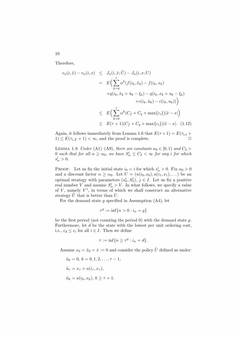
Again, it follows immediately from Lemma 1.6 that E(τ +1) = E(τi,x +1) ≤ E(τi,X + 1) < ∞, and the proof is complete. 2

Lemma 1.8 Under (A1)–(A9), there are constants α0 ∈ [0, 1) and C2 >0 such that for all α ≥ α0, we have Si

α ≤ C2 < ∞ for any i for whichsiα > 0.

Proof. Let us fix the initial state i0 = i for which siα > 0. Fix α0 > 0

and a discount factor α ≥ α0. Let U = (u(i0, x0), u(i1, x1), . . . ) be anoptimal strategy with parameters (sj

α, Sjα), j ∈ I. Let us fix a positive

real number V and assume Siα > V . In what follows, we specify a value

of V , namely V ∗, in terms of which we shall construct an alternativestrategy U that is better than U .

For the demand state g specified in Assumption (A4), let

τ g := infn > 0 : in = g

be the first period (not counting the period 0) with the demand state g.Furthermore, let d be the state with the lowest per unit ordering cost,i.e., cd ≤ ci for all i ∈ I. Then we define

τ := infn ≥ τ g : in = d.

Assume x0 = x0 = x := 0 and consider the policy U defined as under:

uk = 0, k = 0, 1, 2, . . . , τ − 1,

uτ = xτ + u(iτ , xτ ),

uk = u(ik, xk), k ≥ τ + 1.


The two policies and the resulting trajectories differ only in periods 0through τ . Therefore, we have

vα(i, x)− Jα(i, x; U) = Jα(i, x; U)− Jα(i, x; U)

= E( τ∑

k=0




= E( τ∑

k=1

αk(f(ik, xk) + q(ik, xk + uk − ξk)

−q(ik,−ξk)))

+ E

(τ∑

k=0

αkc(ik, uk)

)

−E(ατ c(iτ , uτ )). (1.13)

After ordering in period τ , the total accumulated ordered amount up toperiod τ is less for policy U than it is for U . Observe that the policyU orders only in period τ . The order of the policy U is executed at thelowest possible per unit cost cd in period τ , which is not earlier than anyof the ordering periods of policy U . Because U orders only once and Uorders at least once in periods 0, 1, . . . , τ , the total fixed ordering cost ofU does not exceed the total fixed ordering cost of U . Thus,

E

(τ∑

k=0

αkc(ik, uk)

)≥ E(ατ c(iτ , uτ )).

Furthermore, it follows from Assumptions (A3), (A7), and (A9) that

E

(τ∑

k=1

q(ik,−ξt)

)< ∞.

Because τ ≥ τ g, we obtain

E

(τ∑

k=1

αk(f(ik, xk) + q(ik, xk + uk − ξk))

)≥ E

(τg∑

k=1

αkf(ik, xk)

),

and because Siα ≥ V , we obtain

xk ≥ V −k∑

t=1

ξt.

12

Irreducibility of the the Markov chain (in)∞n=0 implies existence of aninteger m, 0 ≤ m ≤ L, such that P (im = g) > 0. Let m0 be the smallestsuch m. It follows that τ g ≥ m0 and, therefore,

E

(τg∑

k=1

αkf(ik, xk)

)≥ αm0E(f(im0 , xm0))

≥ αm00 E(f(g, V −

m0∑

t=1

ξt)|im0 = g)P (im0 = g),

for all α ≥ α0. (1.14)

Using Assumptions (A2), (A4), and (A9), it is easy to show that theright-hand side of (1.14) tends to infinity as V goes to infinity. Therefore,we can choose V ∗, 0 ≤ V ∗ < ∞, such that for all α ≥ α0,

vα(i, x)− Jα(i, x; U) ≥ αm00 E(f(g, V ∗ −

m0∑

t=1

ξt)|im0 = g)P (im0 = g)

−E

(τ∑

k=1

q(ik,−ξt)

)> 0. (1.15)

Note that the RHS of (1.15) is independent of α. Thus for α ≥ α0, apolicy with Si

α > C2 := V ∗ cannot be optimal. 2

4. Vanishing Discount ApproachLemma 1.9 Under Assumptions (A1)–(A9), the differential discountedvalue function wα(i, x) := vα(i, x) − vα(1, 0) is uniformly bounded withrespect to α for all x and i.

Proof. Since Lemma 1.7 implies

|wα(i, x)| = |vα(i, x)− vα(1, 0)| ≤ |vα(i, x)− vα(i, 0)|+ |vα(i, 0)−vα(1, 0)| ≤ C3|x|+ |wα(i, 0)|,

it is sufficient to prove that wα(i, 0) is uniformly bounded. Note that C3

may depend on x, but it is independent of α.First, we show that there is an M > −∞ with wα(i, 0) ≥ M for

all α. Let α be fixed. From Theorem 1.5 we know that there is astationary discount optimal feedback policy U = (u(i, x), u(i, x), . . . ).With k∗ = infk : ik = i, we consider the cost for the initial state(i0, x0) = (1, 0) and the inventory policy U , which does not order inperiods 0, 1, . . . , k∗ − 1 and follows U beginning with period k∗:


uk = 0 for k < k∗,uk = u(ik, xk) for k ≥ k∗.

The cost corresponding to this policy is

Jα(1, 0; U) = E

(k∗−1∑

k=0

αkq(ik,−ξk) + αk∗vα(i, 0)

). (1.16)

Because of Assumptions (A3), (A7) and (A9),

E

(k∗−1∑

k=0

q(ik,−ξk)

)≤ −M < ∞.

Therefore, we have

wα(i, 0) = vα(i, 0)− vα(1, 0) ≥ vα(i, 0)− Jα(1, 0; U)

≥ vα(i, 0)− E

(k∗−1∑

k=0

αkq(ik,−ξk) + αk∗vα(i, 0)

)

≥ vα(i, 0)(1−E(αk∗)) + M ≥ M. (1.17)

The opposite inequality wα(i, 0) ≤ M is shown analogously by chang-ing the role of the states 1 and i. Thus, |wα(i, x)| ≤ C3|x|+maxM, M,and the proof is complete. 2

Lemma 1.10 Under Assumptions (A3) and (A9), (1−α)vα(1, 0) is uni-formly bounded on 0 < α < 1.

Proof. Consider the strategy U = (0, 0, . . . ). Because U is not neces-sarily optimal,

0 ≤ vα(1, 0) ≤ Jα(1, 0; U) = E

( ∞∑

k=0

αkq(ik,−ξk)

).

Because of (A3) and (A9), Eq(i,−ξk) is bounded for all i and there is aC4 < ∞ such that E(q(ik,−ξk)) < C4. Therefore,

0 ≤ (1− α)vα(1, 0) ≤ (1− α)∞∑

k=0

αkC4 = C4.

This completes the proof. 2

14

Theorem 1.11 Let Assumptions (A1)–(A9) hold. There exist a se-quence (αk)∞k=1 converging to 1, a constant λ∗, and a locally Lipschitzcontinuous function w∗(·, ·) such that

(1− αk)vαk(i, x) → λ∗ and wαk

(i, x) → w∗(i, x),

locally uniformly in x and i as k goes to infinity. Moreover, (λ∗, w∗)satisfies the average cost optimality equation

w(i, x) + λ = f(i, x) + infu≥0

c(i, u) + Eq(i, x + u− ξi) + F (w)(i, x + u).(1.18)

Proof. From Lemma 1.7 and the definition of wα(i, x), it is clearthat wα(i, ·) is locally equi-Lipschitzian for α ≥ α0, and therefore itis uniformly continuous in any finite interval. Additionally, accord-ing to Lemma 1.9, wα(i, ·) is uniformly bounded, and by Lemma 1.10,(1−α)vα(1, 0) is uniformly bounded. Therefore, from the Arzela-AscoliTheorem (see, e.g., ?) and Lemma 1.7, there are a sequence αk → 1,a locally Lipschitz continuous function w∗(i, x), and a constant λ∗ suchthat

(1− αk)vαk(1, 0) → λ∗, and wαk

(i, x) → w∗(i, x)

for each x locally uniformly in any given interval. By the diagonalizationprocedure , a subsequence can be found so that w∗αk

(i, ·) converges to alocally Lipschitz continuous function w∗(i, ·) on the entire real line.

Next, it is easy to see that

limk→∞

(1− αk)vαk(i, x) = lim

k→∞(1− αk)(wαk

(i, x) + vαk(1, 0)) = λ∗.

Substituting vαk(i, x) = wαk

(i, x) + vαk(1, 0) in (1.8) yields

wαk(i, x) + (1− αk)vαk

(1, 0) = f(i, x) + infu≥0

c(i, u)

+Eq(i, x + u− ξi)+αkF (wαk

)(i, x + u). (1.19)

Since wαk(i, x) converges locally uniformly with respect to x and i and

since for a given x, a minimizer u∗ in (1.19) can be chosen such thatx + u∗ − ξ ∈ [0, x + C2] by Lemma 1.8, we can pass to the limit on bothsides of (1.19), and obtain (1.18). This completes the proof. 2

Lemma 1.12 Let λ∗ be defined as in Theorem 1.11. Let Assumptions(A1)–(A9) hold. Then for any admissible strategy U , we have λ∗ ≤J(i, x; U).


Proof. Let U = (u0, u1, . . . ) denote any admissible decision. Suppose

J(i, x; U) < λ∗. (1.20)

Setf(k) = E[f(ik, xk) + q(ik, xk + uk − ξk) + c(ik, uk)].

From (1.20) it follows immediately that∑n−1

k=0 f(k) < ∞ for each positiveinteger n, since otherwise we would have J(i, x; U) = ∞. Note that

J(i, x; U) = lim supn→∞

1n

n−1∑

k=0

f(k),

while

(1− α)Jα(i, x; U) = (1− α)∞∑

k=0

αkf(k). (1.21)

Since f(k) is nonnegative for each k, the sum in (1.21) is well definedfor 0 ≤ α < 1, and we can use the Tauberian theorem (see, e.g., Sznadjerand Filar (1992), Theorem 2.2) to obtain

lim supα↑1

(1− α)Jα(i, x;U) ≤ J(i, x;U) < λ∗.

On the other hand, we know from Theorem 1.11 that (1−αk)vαk(i, x) →

λ∗ on a subsequence αk∞k=1 converging to one. Thus, there exists anα < 1 such that

(1− α)Jα(i, x;U) < (1− α)vα(i, x),

which contradicts the definition of the value function vα(i, x). 2

5. Verification TheoremDefinition 1.13 Let (λ,w) be a solution of the average optimality equa-tion (1.18). An admissible strategy U = (u0, u1, . . . ) is called stable withrespect to w if for each initial inventory level x ≥ 0 and for each initialdemand state i ∈ I,

limk→∞

1kE(w(ik, xk)) = 0,

where xk is the inventory level in period k corresponding to the initialstate (i, x) and the strategy U .

16

Lemma 1.14 Assume (A1)-(A9). There are constants Si < ∞ and 0 ≤si ≤ Si, i ∈ I, such that

u∗(i, x) =

Si − x, x < si

0, x ≥ si

attains the minimum on the RHS in (1.18) for w = w∗ as definedin Theorem 1.11. Furthermore, the stationary feedback strategy U∗ =(u∗, u∗, . . . ) is stable with respect to any continuous function w.

Proof. Let αk∞k=0 be the sequence defined in Theorem 1.11. Let

Gαk(i, y) = ciy + Eq(i, y − ξi) + αkF (wαk

)(i, y)and

G(i, y) = ciy + Eq(i, y − ξi) + F (w∗)(i, y). (1.22)

Because w∗(i, ·) is K-convex, we know that a minimizer in (1.18) isgiven by

u∗(i, x) =

Si − x, x < si

0, x ≥ si ,

where 0 ≤ Si ≤ ∞ minimizes G(i, ·), and si solves

G(si) = K + G(Si),

if a solution exists or else si = 0. Note that if si = 0, it follows thatu∗(i, x) = 0 for all nonnegative x. It remains to show that Si < ∞.

We distinguish two cases.Case 1. If there is a subsequence, still denoted by αk∞k=0, such thatsiαk

> 0 for all k = 0, 1, ..., then it follows from Lemma 1.8 that Gαk

attains its minimum in [0, C2] for all αk > α0. Thus Gαk, k = 0, 1, ..., are

locally uniformly continuous and converge uniformly to G. Therefore,G attains its minimum also in [0, C2], which implies Si ≤ C2.Case 2. If there is no such sequence, then there is a sequence, stilldenoted by αk∞k=0, such that si

αk= 0 for all k = 0, 1, .... It follows

that for all y > x,Gαk

(x) < K + Gαk(y),

and therefore in the limit,

G(x) < K + G(y).

This implies that the infimum in (1.18) is attained for u∗(i, x) ≡ 0, whichis equivalent to si = 0. But, if si = 0, we can choose Si arbitrarily, saySi = C2.


It is immediate that the stationary policy U∗ is stable with respectto any continuous function, since it implies xk ∈ [0, maxC2, x0] for allk = 0, 1, . . . . 2

Theorem 1.15 (Verification Theorem). Let (λ,w(·, ·)) be a solu-tion of the average cost optimality equation (1.18) with w continuous on[0,∞).

(i) Then λ ≤ J(i, x; U) for any admissible U .

(ii) Suppose there exists a u(i, x) for which the infimum in (1.18) isattained. Furthermore, let U = (u, u, . . . ), the stationary feedbackpolicy given by u, be stable with respect to w. Then

λ = J(i, x; U) = λ∗ = limN→∞

1N

E( N−1∑

k=0

f(ik, xk)

+q(ik, xk + uk − ξk) + c(ik, uk)),

and U is an average optimal strategy.

(iii) Moreover, U minimizes

lim infN→∞

1N

E

(N−1∑

k=0

f(ik, xk) + q(ik, xk + uk − ξk) + c(ik, uk)

)

over the class of admissible decisions which are stable with respectto w.

Proof. We start by showing that

λ ≤ J(i, x;U) for any U stable w.r.t. w. (1.23)

We assume that U is stable with respect to w, and begin with a resulton conditional expectations (see, e.g., Gikhman and Skorokhod (1972)),which gives

Ew(in+1, xn+1) | i1, . . . , in, ξ1, . . . , ξn= Ew(in+1, (xn + un − ξn)+)|i1, . . . , in, ξ1, . . . , ξn−1= E(w(in+1, (y − ξn)+)|i1, . . . , in, ξ1, . . . , ξn−1y=xn+un

= E(w(in+1, (y − ξn)+) | iny=xn+un

= F (w)(in, y)y=xn+un

= F (w)(in, xn + un) a.s. (1.24)

18

Because uk does not necessarily attain the infimum in (1.18), we have

w(ik, xk) + λ ≤ f(ik, xk) + c(ik, uk) + q(ik, xk + uk − ξk)+F (w)(ik, xk + uk) a.s.,

and from (1.24) we derive

w(ik, xk) + λ ≤ f(ik, xk) + q(ik, xk + uk − ξk) + c(ik, uk)+E(w(ik+1, xk + uk − ξk+1) | ik) a.s..

By taking the mathematical expectation on both sides, we obtain

E(w(ik, xk)) + λ ≤ E(f(ik, xk) + q(ik, xk + uk − ξk) + c(ik, uk))+E(w(ik+1, xk+1)).

Summing from 0 to n− 1 yields

nλ ≤ E

(n−1∑

k=0


)

+E(w(in, xn))− E(w(i0, x0)). (1.25)

Divide by n, let n go to infinity, and use the fact that U is stable withrespect to w, to obtain

λ ≤ lim infn→∞

1n

E

(n−1∑

k=0


).

(1.26)Note that if the above inequality holds for ‘liminf’, it certainly holds alsofor ‘limsup’. This proves (1.23).

On the other hand, if there exists a u which attains the infimum in(1.18), we then have

w(ik, xk) + λ = f(ik, xk) + q(ik, xk + uk − ξk) + c(ik, u(ik, xk))+F (w)(ik, xk + u(ik, xk)), a.s.,

and we obtain analogously

nλ = E

(n−1∑

k=0

f(ik, xk) + q(ik, xk + uk − ξk) + c(ik, u(ik, xk))

)

+E(w(in, xn))−E(w(i0, x0)). (1.27)

Because U is assumed stable with respect to w, we get

λ = limn→∞

1n

E

(n−1∑

k=0

f(ik, xk) + q(ik, xk + uk − ξk) + c(ik, u(ik, xk)

)

= J(i, x; U). (1.28)


For the special solution (λ∗, w∗) defined in Theorem 1.11 and thestrategy U∗ defined in Lemma 1.14, we obtain

λ∗ = J(i, x;U∗).

We know from Lemma 1.14 that U∗ is stable with respect to any con-tinuous function. It therefore follows that

λ ≤ J(i, x;U∗) = λ∗, (1.29)

which, in view of Lemma 1.12, proves part (i) of the theorem.Part (i) of the Theorem together with (1.28) proves the average-

optimality of U over all admissible strategies. Furthermore, since λ =J(i, x; U) ≥ λ∗ by (1.28) and Lemma 1.12, it follows from (1.29) thatλ = λ∗ and the proof of Part (ii) is completed.

Finally, Part (iii) immediately follows from Part (i) and (1.26). 2

Remark 1.16 It should be obvious that any solution (λ,w) of the av-erage cost optimality equation and control u∗ satisfying (i) and (ii) ofTheorem 1.15 will have a unique λ, since it represents the minimumaverage cost. On the other hand, if (λ,w) is a solution, then (λ,w + c),where c is any constant, is also a solution. For the purpose of this paperwe do not require w to be unique up to a constant. If w is not uniqueup to a constant, then u∗ may not be unique. We also do not need w∗in Theorem 1.11 to be unique either.

The final result of this section, namely, that there exists an average-optimal policy of (s, S)-type is an immediate consequence of Lemma 1.14and Theorem 1.15.

Theorem 1.17 Assume (A1)–(A9). Let si and Si, i ∈ I, be definedas in Lemma 1.14. The stationary feedback strategy U∗ = (u∗, u∗, . . . )defined by

u∗(i, x) =

Si − x, x < si

0, x ≥ si,

is average optimal.

6. Concluding RemarksIn this paper we have carried out a rigorous analysis of the average cost

stochastic inventory problem with Markovian demand, fixed orderingcost and lost sales. We have proved a verification theorem for the averagecost optimality equation, which we have used to establish the existenceof an optimal state-dependent (s, S)-policy.

20

Throughout the analysis, we have assumed that the inventory andshortage cost functios are of linear growth. Further research shouldaddress extending this analysis to more general cost functions. An ex-tension of the model for cost functions with polynomial growth in thebacklog case was carried out in Beyer, Sethi and Taksar (1998). Forother extensions, see the forthcoming book by Beyer, Cheng and Sethi(2004).

ReferencesBensoussan, A., Crouhy, M., and Proth, J. Mathematical Theory of

Production Planning. North-Holland, 1983.Beyer, D. and Sethi, S.P. Average Cost Optimality in Inventory Mod-

els with Markovian Demand. Journal of Optimization Theory andApplications, 92:3,497–526, 1997.

Beyer, D. and Sethi, S.P. The Classical Average-Cost Inventory Modelsof Iglehart and Veinott-Wagner Revisited. Journal of OptimizationTheory and Applications, 101:3,523-555, 1999.

Beyer, D., Sethi, S.P., and Taksar, M. Inventory Models with Marko-vian Demands and Cost Functions of Polynomial Growth. Journal ofOptimization Theory and Application, 98:2,281–323, 1998.

Beyer, D., Cheng, F., and Sethi, S.P. Inventory Models in MarkovianEnvironments. Kluwer, forthcoming.

Cheng, F., and Sethi, S.P. Optimality of State-Dependent (s, S) Policiesin Inventory Models with Markov-Modulated Demand and Lost Sales.Production and Operations Management, 8:2,183–192, 1999.

Federgruen, A. and Zipkin, P. An Efficient Algorithm for ComputingOptimal (s, S) Policies. Operations Research, 32:1268–1285, 1984.

Feller, W. An Introduction to Probability Theory and its Application.Vol. 2, 2nd Edition, Wiley, New York, NY, 1971.

Gikhman, I., and Skorokhod, A. Stochastic Differential Equations. SpringerVerlag, Berlin, Germany, 1972.

Karlin, S., and Fabens, A. The (s, S) Inventory Model under MarkovianDemand Process. Mathematical Methods in the Social Sciences, editedby K. Arrow, S. Karlin, and P. Suppes, Stanford University Press,Stanford, CA, 159–175, 1960.

Ozekici, S., and Parlar, M. Inventory Models with Unreliable Suppliersin Random Environment. Annals of Operations Research, 91:123–136,1999.

Scarf, H. The Optimality of (s, S) Policies in the Dynamic InventoryProblem. Mathematical Methods in the Social Sciences, edited by


K. Arrow, S. Karlin, and P. Suppes, Stanford University Press, Stan-ford, CA, 196–202, 1960.

Sethi, S.P. and Cheng, F. Optimality of (s, S) Policies in Inventory Mod-els with Markovian Demand Processes. Operations Research, 45:6,931–939, 1997.

Shreve, S.E. Abbreviated proof [in the lost sales case] in Bertsekas, D.P.Dynamic Programming and Stochastic Control, Academic Press, NewYork, NY, 105–106, 1976.

Song, J.S., and Zipkin, P.Inventory Control in a Fluctuating DemandEnvironment. Operations Research, 41:351–370, 1993.

Sznadjer, R. and Filar, J. A., Some Comments on a Theorem of Hardyand Littlewood. Journal of Optimization Theory and Applications,75:1,201–208, 1992.

Veinott, A. On the Optimality of (s, S) Inventory Policies: New Con-ditions and a New Proof. SIAM Journal on Applied Mathematics,14:5,1067–1083, 1966.

chapter 1sethi/postscript/lost sales template.pdfchapter 1 average cost optimality in inventory...

Documents