chapter 1 structure of lie algebraspersonalpages.to.infn.it/~billo/didatt/gruppi/liealgebras.pdf ·...

Chapter 1

STRUCTURE OF LIE ALGEBRAS

1.1 Introduction

In this Chapter ...Goal of classifying the complexified Lie algebras. As for groups, try to sinle out “build-

ing blocks”, that will be (semi)-simple Lie algebras. Classification of complex simple algebrascompletely known, 4 families plus 5 exceptional cases. ...

1.1.1 Complexified Lie algebras

A complex or complexified Lie algebra Gc is a Lie algebra that as a vector space is defined overC. The generators can be linearly combined with complex coefficients, and changes of basis areeffected by complex matrices in GL(n,C). Therefore, more sets of structure constants are relatedby a change of basis, and the classes of isomorphic algebras are larger.

Example The complexification of the Lie algebra of real matrices gl(n,R) is, of course, the Liealgebra of complex matrices gl(n,C); similarly the algebra of complex traceless matrices gl(n,C)is the complexification of sl(n,R).

Consider the algebra sl(2,C), whose elements are matrices of the form

m = m0 L0 +m+ L+ +m− L− , m0,m±1 ∈ C , (1.1.1)

where the generators L0 and L± were introduced in Eq. (??).The Lie algebra sl(2,C) is isomorphic to the complexification of the Lie algebra su(2), defined

in Eq.s (??,??) which, in turn, was already isomorphic as a real Lie algebra to so(3). Indeed,the generators L0, L± are related by a complex change of basis to the generators ti = −i/2σ

i ofsu(2):

L0 = σ3 = 2i t3 ,

L± =σ1 ± iσ2

2= i(t1 ± it2) . (1.1.2)

The inverse relation is that

t3 = −i

2L0 ,

t1 = −i

2(L+ + L−) ,

1

Some important structures in Lie algebras 2

t2 = −1

2(L+ − L−) . (1.1.3)

Thus the complex algebra sl(2,C) admits different real sections, namely different real Liealgebras obtained by taking real linear combinations of three independent generators, chosen ascertain specific (in general complex) combinations of the L0, L± generators. If we allow onlyreal linear combinations of L0, L± we obtain sl(2,R); if we allow only real combinations of thegenerators ti of Eq. (??) we obtain su(2). As an exercise, define the real section that leads to theLie algebra su(1, 1) (the Lie algebra of the group SU(1, 1)).

1.1.1.1 Real sections

... choice of an involutive automorphism.

1.2 Some important structures in Lie algebras

...

1.2.1 Subalgebras and ideals

Let us investigate the most important substructures that may appear in a Lie algebra G. Wewill remark the relations of these substructures to substructures of the Lie group that is obtainedunpn exponentiation of G. We will in particular introduce the notions of Lie subalgebra and ofideal.

1.2.1.1 Lie subalgebras

Given a Lie algebra G, a subspace H ⊂ G is a Lie subalgebra of G iff it is by itself a Lie algebra.Namely, we must have (in symbolic notation):

[H,H] ⊆ H . (1.2.4)

Under the exponential map, a Lie subalgebra generates a Lie subgroup:

H ⊂ G exp−→ H = eH ⊂ G = eG , (1.2.5)

with H a subgroup of G. Indeed, ∀x, y ∈ H, the group product of the correponding groupelements:

exey = exp

(

x+ y +1

2[x, y] +

1

12([x, [x, y]] + [[x, y] , y]) + . . .

)

= ez , with z ∈ H , (1.2.6)

where we used the Baker-Campbell-Hausdorff formula Eq. (??). Indeed, the result of all commu-tators above stay in H, by the definition Eq. (1.2.4).

Every generator L of a Lie algebra gives rise to an abelian subalgebra {λL}, with λ ∈ R,that exponentiates to a one-parameter abelian subgroup of G.


1.2.1.2 Ideals

An ideal I ⊂ G is a subalgebra such that

[I,G] ⊆ I . (1.2.7)

That is, commuting an element of I with any element of G we obtain again an element of I *ingeneral a different one).

An ideal of G exponentiates to an invariant subgroup

I = eI ⊂ G (1.2.8)

of G. Indeed, ∀h ∈ I, ∀x ∈ G, we have

e−xehex = exp(

e−xhex)

= exp

(

h− [x, h] +1

2[x, [x, h]] + . . .

)

= eh′

, with h′ ∈ I . (1.2.9)

We used the properties Eq.s (??,??) of the exponential map, and the fact that [x, h] ∈ I, so thatalso [x, [x, h]] ∈ I, and so on.

Let us note a couple of simple properties of ideals.

i) If I, I ′ are ideals of G, then also I + I ′ (i.e. the subspace obtained as the direct sum of thesubspaces I and I ′) is an ideal. Indeed, ∀x ∈ I, ∀x′ ∈ I ′ and ∀y ∈ G, we have

[x+ x′, y] = [x, y] + [x′, y] ∈ I + I ′ , (1.2.10)

since [x, y] ∈ I and [x′, y] ∈ I ′.ii) If I, I ′ are ideals of G, then also [I, I ′] (namely the subspace spanned by all commutators

between elements of the two ideals) is an ideal. Indeed, ∀x ∈ I, ∀x′ ∈ I ′ and ∀y ∈ G, wehave, using the Jacobi identity,

[[x, x′] , y] = − [[x′, y] , x]− [[y, x] , x′] ∈ [I, I ′] , (1.2.11)

since [x, y] ∈ I and [x′, y] ∈ I ′.

1.2.1.3 Center of a Lie algebra

The center Z(G) of a Lie algebra G is the subalgebra such that

[Z(G),G] = 0 . (1.2.12)

Elements of the center of the Lie algebra exponentiate to elements in the center of the Liegroup G: ∀z ∈ Z(G), ∀y ∈ G,

e−yezey = exp(

e−yzey)

= exp

(

z − [z, x] +1

2[y, [y, z]] + . . .

)

= ez , (1.2.13)

all the commutator terms vanish because of Eq. (1.2.12).


1.2.1.4 The derived algebra

The derived algebra DG of a Lie algebra G is the subspace spanned by all commutators:

DG = [G,G] . (1.2.14)

The derived algebra exponentiates to the derived group DG, namely the group generated by allgroup commutators. In fact, every group commutator in G can be written as follows:

exeye−xe−y = exp(

exye−x)

e−y = exp (y + comm.s) e−y = exp (comm.s) = ez , z ∈ DG .(1.2.15)

The derived algebra DG is clearly an ideal of G, as [DG,G] ⊆ DG by the definition Eq. (1.2.14).Let us further notice the following simple facts.

i) If G is Abelian, we obviously have DG = 0;ii) At the opposite, there are many instances of Lie algebras such that DG = G, namely, all

elements can be written as commutators. For instance, in the su(2) algebra we have

t1 = [t2, t3] , t2 = [t3, t1] , t3 = [t1, t2] . (1.2.16)

1.2.1.5 Normalizer

The normalizer N (K) of a subspace K ⊂ G is the subspace of G for which K behaves like anideal:

N (K) = {x ∈ G : [K,x] ⊆ K} . (1.2.17)

The normalizer N (K) is a subalgebra of G. Indeed, using the Jacobi identity we have, ∀x, y ∈N (K),

[K, [x, y]] = − [x, [y,K]]− [y, [K,x]] ∈ K , (1.2.18)

since in the r.h.s. the commutators [y,K] and [K,x] belong to K because of the definitionEq. (1.2.17), and so do then the double commutators.

A normalizer in the Lie algebra G exponentiates to a normalizer in the Lie group G.

1.2.1.6 Centralizer

The centralizer C(K) of a subspace K ⊂ G is the subspace of G for which K behaves like thecentre:

C(K) = {x ∈ G : [K,x] = 0} . (1.2.19)

The normalizer C(K) is a subalgebra of G. Indeed, using the Jacobi identity we have, ∀x, y ∈C(K),

[K, [x, y]] = − [x, [y,K]]− [y, [K,x]] = 0 , (1.2.20)

as it follows from immediately using in the r.h.s. the Eq. (1.2.17), and so do then the doublecommutators.

A Lie algebra centralizer exponentiates to a centralizer in the Lie group G.


1.2.2 Quotient Lie algebras

The quotient space

G/I (1.2.21)

of a Lie algebra G by an ideal I ⊂ G is again a Lie algebra. In Eq. (1.2.21) G/I, as a vectorspace, is just the usual quotient space with respect to the equivalence relation

∀x, x′ ∈ G , x ∼ x′ ⇔ x′ = x+ u , for some u ∈ I . (1.2.22)

The elements of G/I are the equivalence classes with respect to Eq. (1.2.22), which we maydenote as [x] ≡ x+ I. The dimension of G/I is

dimG/I = dimG− dim I . (1.2.23)

The Lie product of the classes is simply defined as

[x+ I, y + I] ≡ [x, y] + I . (1.2.24)

This is a good definition, namely it is independent of the choice of representatives x, y preciselybecause I is in ideal. Indeed, choosing any other representatives x′ = x + u, y′ = y + v, withu, v ∈ I, we have

[x′, y′] = [x+ u, y + v] = [x, y] + w , with w = [u, y] + [x, v] + [u, v] ∈ I . (1.2.25)

Therefore we find

[x′ + I, y′ + I] = [x, y] + I = [x+ I, y + I] . (1.2.26)

Equipped with the Lie product Eq. (1.2.24) the quotient space is thus a Lie algebra.Upon exponentiation, the quotient algebra gives rise to a factor group:

G/I exp−→ exp (G/I) = G/I , (1.2.27)

where I is the normal subgroup of G = expG obtained exponentiating the ideal I. Indeed, theequivalence relation Eq. (1.2.22) gives rise to the (left) equivalence relation in the group, seeEq. (??) which is used to define G/I: if x′ ∼ x, namely if x′ = x+ u for some u ∈ I, then

ex+u = ex exp

(

u−1

2[x, u] + . . .

)

= ex h with h′ = eu′

∈ I , (1.2.28)

since u′ ∈ I as all the commutators in the exponent belong to I by the definition of ideal. Thusthe classes x+I exponentiate to the classes ex I, namely the elements of G/I. Since I is a normalsubgroup, G/I is a group.

1.2.2.1 First homomorphism theorem

The first homomorphism theorem for groups, discussed in Sec. ?? has a counterpart for Liealgebras. Let

φ : G −→ G′ (1.2.29)

be a Lie algebra homomorphism.


i) kerφ is an ideal of G. Indeed, ∀x ∈ kerφ, ∀y ∈ G,

φ ([x, y]) = [φ(x), φ(y)] = [0, φ(y)] = 0 , (1.2.30)

so that [x, y] belongs to kerφ as well.ii) We can thus form the quotient algebra G/kerφ. When restricted to the quotient algebra, φ

becomes an isomorphism:φ : G/kerφ←→ G′ . (1.2.31)

The above is an example of the more general relation between homomorphisms (and iso-morphisms) at the group and algebra level. The main idea (which we state without discussion)is the following. Let G1, G2 be two Lie groups, and G1,G2 their Lie algebras. In general, thegroup of group homomorphisms Hom(G1, G2) is mapped homomorphically onto the group of Liealgebra homomorphisms hom(G1,G2). The map is an isomorphism only when G1 and G2 aresimply-connected.

1.2.3 Adjoint action and adjoint map (or representation)

1.2.3.1 Adjoint action of the group on the algebra

Every element g of a Lie group G determines an automorphism Adg of the associated Lie algebraG, given as follows:

∀x ∈ G , Adg : x 7→ g−1xg ∈ G . (1.2.32)

Indeed, writing g = ey, with y ∈ G, we see that

e−yxey = x− [y, x] +1

2[y, [y, x]] + . . . ∈ G . (1.2.33)

The map Adg is an homomorphism since, ∀x, y ∈ G,

[

g−1xg, g−1yg]

= g−1xgg−1yg − (x↔ y) = g−1 [x, y] g . (1.2.34)

It is in fact also an isomorphism, as the kernel coincides with 0: asking that g−1xg = 0 impliesthat x = 0.

We made use of the adjoint action of the group in Sec. ?? when we discussed the homomor-phic relation between SU(2) and SO(3).

1.2.3.2 The adjoint map (or adjoint representation) of a Lie algebra

The adjoint map ad associates to every element x in a Lie algebra G a linear operator adx ∈End(G) acting on G itself, defined as follows:

adx : y ∈ G 7→ adxy = [x, y] . (1.2.35)

This map is an homomorhism of the Lie algebra into itself, namely we have

[adx, ady] = ad[x,y] , (1.2.36)

where the commutator in the l.h.s. is a commutator of linear operators. Indeed, ∀z ∈ G,

[adx, ady] z = adx [y, z]− ady [x, z] = [x, [y, z]]− [y, [x, z]] = − [x, [z, y]]− [y, [x, z]]

= [z, [y, x]] = [x, [y, z]] = ad[x,y]z . (1.2.37)


Thus the adjoint map gives in fact a d-dimensional representation of the Lie algebra G,where d = dimG. The explicit matrix representatives can be written choosing a basis {ti} ofgenerators. One has then

adtitj = [ti, tj ] = c kij tk , (1.2.38)

namely the generators in this prepresntation are given by

(Ti)kj ≡ (adti)

kj = c k

ij . (1.2.39)

This is nothing else but the definition of the adjoint representation given in Sec. ??.The kernel of the adjoint map is the center of the algebra: x ∈ ker ad iff adxy = [x, y] = 0

for every y ∈ G, namely iff x ∈ Z(G). Thus the adjoint representation is faithful only if G has atrivial center.

1.2.3.3 Derivations of a Lie algebra

A derivation of a Lie algebra is an operator ∂ : G→ G satisfying the following properties.

i) Linearity: ∂(αx+ βy) = α∂x+ β∂y, where x, y ∈ G and α, β are scalar coefficients.ii) Leibnitz rule:

∂ [x, y] = [∂x, y] + [x, ∂y] . (1.2.40)

This concept is perfectly analogous to the concept of derivation of an algebra, discussed in themathematical Appendix, Sec. ??, around Eq. (??), where we regarded tangent vectors and vecorfields as derivations of the algebra of locally and globally defined functions respectively. Weremarked that the space ∂A of derivations of an algebra A is a Lie algebra, see Eq. (??). Thefact that the vector fields form a Lie algebra played an important role in our discussion of therelation between Lie groups and Lie algebras in Sec. ??. Similarly, the space ∂G of derivationsof a Lie algebra forms a Lie algebra. Show this directly as an exercise.

The adjoint operators adx are derivations of G: ∀x ∈ G, adx ∈ G (so ∂G is at least as bigas G. Indeed, linearity is immediate, and the Leibnitz rule follows from the Jacobi identity:

adx [y, z] = [x, [y, z]] = − [y, [z, x]]− [z, [x, y]] = [[x, y] , z] + [[y, x] , z] = [adxy, z] + [y, adxz] .(1.2.41)

1.2.4 Direct and semi-direct sums of Lie algebras

1.2.4.1 Direct sum of Lie algebras

We say that G is the direct sum of G1 and G2, and we denote it as

G = G1 ⊕G2 , (1.2.42)

if the following is true:

i) G as a vector space is the direct sum of G1 and G2;ii) G1 and G2 are both ideals of G:

[G1,G1 ⊕G2] ⊆ G1 ,

[G2,G1 ⊕G2] ⊆ G2 (1.2.43)

from which it follows that all the “mixed” commutators vanish: [G1,G2] = 0.


1.2.4.2 Semi-direct sum of Lie algebras

Let K and H be Lie algebras. Suppose that K admits a representationσ by means of linearoperators acting on H:

∀k ∈ K , σ : k −→ σ(k) ∈ H . (1.2.44)

Suppose moreover that all these operators σ(k) be derivations of H. We define then the semi-direct sum Lie algebra

G = K⊕s H (1.2.45)

as the Lie which

i) as a vector space is simply the direct sum of K and H, so that its elements can be simplydenoted as k + h, with k ∈ K and h ∈ H;

ii) is endowed with the Lie product

[k + h, k′ + h′] ≡ [k, k′] + [h, h′] + σ(k)h′ − σ(k′)h . (1.2.46)

Notice that the first term in the r.h.s. is in K, all the remaining ones on H. Eq. (1.2.46) is agood definition of a Lie product, as it satisfies the necessary properties: linearity and Jacobiidentity. Linearity is immediate, Jacobi identity is left as an exercise (it is in verifying theacobi identity that the fact that σ(k) is a derivation comes into play).

In the reverse direction, when can we assert that a Lie algebra G decomposes into a semidirectsum? It must be the case that G decomposes as a vector space as G = K⊕H and

i) K ∩ H = 0, so that any element g ∈ G is uniquely written as g = k + h, with k ∈ K andh ∈ H;

ii) H is an ideal of G.

This being the case, we have G = K⊕s H, with the original Lie product in G. Indeed, we have

[k + h, k′ + h′] = [k, k′] + [h, h′] + [k, h′]− [k′, h] (1.2.47)

which agrees with Eq. (1.2.46) with the representation σ of K being provided by the adjoint map:σ(k) = adk. Indeed, since H is an ideal, we have in particular [K,H] ⊆ H, so that every adk is alinear operator acting on H

Under the exponential map, a semidirect sum maps to a semi-direct product of Lie groups:

G = K⊕s H exp−→ G = KsH , (1.2.48)

where H = expH is an invariant subgroup of G. The unicity of the decomposition at the algebralevel maps into the unicity of the decomposition g ∈ G = gg, with g ∈ K, g ∈ H, and thederivation σ defines upon exponentiation the “adjoint” action of K on H which is inherent tothe definition of the semi-direct product of groups, see Eq. (??).

Example of a direct sum Lie algebra: so(4) ∼ so(3) ⊕ so(3) We defined in Eq. (??) a basisof generators Lab = −Lba (a < b) for the so(n) algebra. The six so(4) generators Lab, witha, b,= 1, 2, 3, 4 satify the algebra Eq. (??), for n = 4:

[Lab, Lcd] = δadLbc + δbcLad − δacLbd − δbdLac . (1.2.49)

The main types of Lie algebras 9

We can immediately individuate a so(3) subalgebra spanned by the three generators Lij , wherei, j run only up to 3. Viewing the Lab as 4 × 4 matrices, the Lij are nothing else but the usual3 × 3 generators of so(3) placed in the upper left 3 × 3 block. As usual for so(3) let us renamethese generators as

Mi =1

2εijkLjk (i, j = 1, 2, 3) . (1.2.50)

These generators close evidently a so(3) subalgebra:

[Mi,Mj ] = εijkMk . (1.2.51)

The remaining set of three generators we denote as follows:

Ni = Li4 (i = 1, 2, 3) . (1.2.52)

From Eq. (1.2.49), beside Eq. (1.2.52), the following commutation relations arise (check it):

[Ni, Nj ] = − εijkMk ;

[Mi, Nj ] = εijkNk . (1.2.53)

With the following real change of basis:

Ji =Mi +Ni

2,

Ki =Mi −Ni

2, (1.2.54)

it is possible to disentangle the commutation relations Eq.s (1.2.52,1.2.53); the Lie algebra so(4),expressed in the basis of geberators Ji,Ki, exhibits a direct product structure (check it):

[Ji, Jj ] = εijkJk ;

[Ki,Kj ] = εijkKk . (1.2.55)

hus we have so(4) = so(3) ⊕ so(3), the two so(3) factors being generated respectively from thema and the Na.

1.3 The main types of Lie algebras

The basic insight in trying to study and classify the possible Lie algebras is to analyze first theirpossible structure of ideals; as we have seen, when non-trivial ideals are present, this indicatesthat the algebra can be seen as being obtained as an “extension” by means e.g. of direct orsemidirect sums from simpler algebras.

Let us start from some definitions that are appropriate to this task.

1.3.1 Simple Lie algebras

A Lie algebra G is simple iff

i) G admits no ideals;ii) the derived algebra DG ≡ [G,G] is non trivial.


The requirement ii) excludes the Abelian algebras from the class of simple Lie algebras, which byrequirement i) are defined indeed as the “simplest” Lie algebras, not admitting any substructurefrom which they could be determined as direct or semi-direct extensions.

Notice that if G is simple, then

DG = G (1.3.56)

as otherwise G would contain a proper ideal DG. Also, if G is simple, its center Z(G) must betrivial, for the same reason.

The exponential of a simple Lie algebra G gives a simple group G = expG (if with G wedenote the unique simply-connected group obtained upon exponentiation).

1.3.2 Nilpotent and solvable algebras

Simple Lie algebra have the property Eq. (1.3.56) that the derived algebra coincides with thealgebra, namely that all elements can be expressed as commutators. We now introduce classesof algebras (nilpotent and solvable Lie algebras) that have in a way the opposite behaviour. Theconcepts of nilpotent and solvable algebras, and the contrasting one of semi-simple algebras wewill introduce after, are basically extensions to entire Lie algebras of well known concepts forendomorphisms, that are very briefly summarized in Sec. ?? of the appendix.

1.3.2.1 Nilpotent Lie algebras

A Lie algebra G is a nilpotent Lie algebra if it possesses a terminating central descending seriesof ideals:

G ≡ G1 ⊃ G2 ≡[

G1,G1]

⊃ G3 ≡[

G1,G2]

⊃ . . . ⊃ Gk = {0} , (1.3.57)

for some k ∈ N.

The typical example of a nilpotent Lie algebra is the Lie algebra N(k,R) of strictly uppertriangular N ×N matrices: ∀m ∈ N(N,R), mij 6= 0⇒ j > i. It is then clear that in the productof any such matrices (and thus also in their commutator) also all the elements immediatly abovethe diagonal vanish: (mn)ij 6= 0⇒ j > i+1, and so on. Thus the subspaces of matrices Ni(k,R)which are non-zero only from i lines above the diagonal on form a terminating chain of ideals asin Eq. (1.3.57) with k = N , since

[

N(N,R),Ni(N,R)]

= Ni+1(N,R) (1.3.58)

and clearly NN (N,R) contains only the null matrix.

Notice however that it is not necessary that G to be made of nilpotent operators for it tobe a nilpotent algebra. Indeed, a simple counterexample is the Lie algebra of diagonal k × kmatrices, D(N,R) which is clearly Abelian (and isomorphic to RN ):

[D(N,R),D(N,R)] = 0 , (1.3.59)

and thus exhibits the property Eq. (1.3.57) with k = 0.

The point is that the property Eq. (1.3.57) actually concernes the adjoint representation ofthe Lie algebra G.


Engel’s theorem Indeed, the definition Eq. (1.3.57) has the following meaning. For some k, thatdepends only on the algebra G, we have

adx1adx2 . . . adxk

(y) = 0 ∀xi, y ∈ G . (1.3.60)

In particular, as an operator,(adx)

k = 0 ∀x ∈ G , (1.3.61)

that is, all the adjoint operators adx are nilpotent endomorphisms, The converse (if all the adjointoperators adx are nilpotent then the algebra G has the property Eq. (1.3.57)) turns also out tobe true, so we have the so-called Engel’s theorem:

G nilpotent ⇔ ∀x ∈ G , adx ∈ End(G) is nilpotent. (1.3.62)

The chain property Being nilpotent, all operators adx admit a common null eigenvector, andwith an appropritate choice of basis {ti} of G they are represented by strictly upper triangularmatrices. In this basis, G admits a chain of ideals of codimension 1:

G1 ≡ G ⊃ G2 ⊃ . . . ⊃ Gd = {0} , (1.3.63)

where d = dimG, G = G1 is spanned by the generators {ti}, with i = 1, . . . d, G2 is spanned by{ti} with i = 1, . . . d− 1 and so forth. We have dimGn = d− n− 1 and (by the same reasoningwe used to obtain Eq. (1.3.58))

∀x ∈ G , adx : Gk −→ Gk+1 , i.e.,[

G,Gk]

⊂ Gk+1 . (1.3.64)

The chain of ideals Eq. (1.3.63) “majorizes” the central descending series Eq. (1.3.57).

Some properties of nilpotent Lie algebras

i) If G is nilpotent, all subalgebras and homomorphic images of G are nilpotent as well.ii) If G/Z(G is nilpotent, then G is nilpotent (show this as an exercise).iii) If G is nilpotent (and non-trivial), then it has a non-trivial center. Indeed, the last term in

the central descending series Eq. (1.3.57) is central:[

G,Gk−1]

= 0.

1.3.2.2 Solvable Lie algebras

Nihilpotent algebras are defined by the property Eq. (1.3.57). We have seen that this implies thechain property Eq. (1.3.63), but is in fact a stronger condition the reverse implication does nothold).

Now we externd our attention to the most general Lie algebras that admit a chain of codi-mension 1 ideals as in Eq. (1.3.63) (or, briefly. “have the chain property”). Such algebras arenamed solvable Lie algebras.

The name is due to the fact that under the exponential map, a solvable Lie algebra gives riseto a solvable Lie group. Indeed, referiing to the chain Eq. (1.3.63), the quotient algebra Gk/Gk+1

has dimension 1, hence it is Abelian. For the Lie group G = expG we obtain a chain of invariantsubgroups:

G1 ≡ G ⊃ G2 ⊃ . . . ⊃ Gd = {e} (1.3.65)

with all the factor groups Gk/Gk+1 having dimension 1, and hence being Abelian. According tothe definition given in Sec. ??, G is solvable.


It is possible to define the solvability in a different way, by means of a property similarto (but less restrictive than) the property Eq. (1.3.57) that defines the nilpotent algebras. Analgebra G is solvable iff it possesses a terminating derivative series:

G ⊃ DG ⊃ D2G ⊃ . . . ⊃ DkG = {0} , (1.3.66)

for some k ∈ N. The properties Eq. (1.3.65) and Eq. (1.3.66) are equivalent. Assume Eq. (1.3.65).Since G admits a proper ideal G2, it can be shown that DG 6= G: the algebra is not simple. Thedimension of DG must therefore be at least 1 less than the dimension of G, so DmathbbG ⊆ G2.The reasoning can be repeated for G2, which admits the proper ideal G3, so that DG2 = D2G ⊆G3, and so on. Thus the chain Eq. (1.3.65) majorizes the derivative series Eq. (1.3.66); since theformer stops at some point, so does the second. In the reverse direction, assume Eq. (1.3.66).Since DG ⊂ G is a proper ideal, there is a subset of generators of G ,{ti} with i = 1, . . . p,which are outside DG. Let us adjoin all these generators but one to DG, namely let us constructG ⊕ Span(t1, . . . , tp−1). This subspace is an ideal since it contains DG, and has codimension 1.The argument can be repeated, so that the series Eq. (1.3.65) can be constructed.

The solvable Lie algebras are characterized by the fact that

i) all the adjoint operators adx, ∀x ∈ G admit a common eigenvector (in general, a non-nullone);

ii) there exists a basis of G in which all the matrices adx have an upper (not strictly upper,in general) triangular form. This is true at the level of complexified algebras, the change tosuch a basis is in general complex.

Some important properties of solvable algebras are listed below.

i) If G is solvable, DG is nilpotent.ii) If G is solvable, so are all its subalgebras and homomorphic images.iii) If I ⊂ G is a solvabe ideal and G/I is solvable, then G is solvable.iv) If I and I ′ are solvable ideals of some Lie algebra G, then I + I ′ is a solvable ideal of G.

The typical model of a solvable Lie algebra is the Lie algebra M(N,R) of N × N uppertriagular matrices: ∀m ∈ M(N,R), mij 6= 0 ⇔ j ≥ i. The product of two such matrices isstill upper triangular, but any commutator [m,n] is strictly upper triangular (the terms on thediagonal cancel):

[M(N,R),M(N,R)] = N(N,R) (1.3.67)

where N(N,R) is the nilpotent Lie algebra of strictly upper triangular matrices described afterEq. (1.3.57). The central descending series Eq. (1.3.57) for M(N,R) does not terminate, since ifwe now commute an element m of M(N,R), mij 6= 0 ⇔ j ≥ i, with a strictly upper triangularmatrix n ∈ N(N,R), nij 6= 0⇔ j > i, we get [m,n]ij 6= 0⇔ j > i, i.e.

[M(N,R),N(N,R)] = N(N,R) , (1.3.68)

and the descending series does not proceed further. However, the derivative series Eq. (1.3.66)does terminate: the commutators of commutators become “more and more upper-triangular”.

Example A simple example of a solvable Lie algebra is given by the Lie algebra iso(2) of theinhomogeneous proper rotation group ISO(2), taht we discussed in Sec. ??. The group ISO(2)is the group of transformations of the space R2 described by Eq. (??): x 7→ R(θ)x + v, whereR(θ) ∈ SO(2) and x ≡ (x1, x2) ∈ R2. It is a 3-dimensional Lie group, parametrized by the three


coordinates θ ∈ [0, 2π] and vi ∈ R, i = 1, 2. The generators of infinitesimal tranformations T1

and T2, associated to infinitesimal tranformations δv1 and δv2 respectively, and T3, associated toδθ, accordingly to Eq. (??) are immediately found to be given by

T1 =∂

x1, T2 =

∂

x2, T3 = x2 ∂

x1− x1 ∂

x2. (1.3.69)

T3 is indeed (−i times) the angular momentum in the x1, x2 plane, see Eq. (??), while T1,2 are (itimes) the momenta in the two directions. Their commutators are easily found:

[T1, T2] = 0 , [T3, T1] = T2 , [T3, T2] = −T1 . (1.3.70)

The subalgebra spanned by T1,2 is just the algebra of infinitesimal two-dimensional translationsT2 ∼ R2, which is Abelian.

Changing basis by introducing T± = T2 ± iT1, the commutation relations become

[T+, T−] = 0 , [T3, T±] = ±iT± . (1.3.71)

The commutations define the form of the adjoint endomorphisms:

adTiTj ≡ [Ti, Tj ] = (adTi

)kj Tk . (1.3.72)

With the basis ordering (T3, T+, T−) Eq. (1.3.71) implies thus

adT3=

0 0 00 i 00 0 i

, adT+=

0 −i 00 0 00 0 0

, adT− =

0 0 i0 0 00 0 0

. (1.3.73)

All the adjoint matrices are upper triangular. On the other hand, the algebra iso(2) is immediatelyseen to be solvable according to the definition Eq. (1.3.66). The central descending series is

iso(2) ⊃ Diso(2) ≡ [iso(2), iso(2)] = T2 ⊃ D2iso(2) ≡ [T2, T2] = 0 . (1.3.74)

Indeed, it follows from Eq. (1.3.69) that only the generators T1,2 are exrpessible as commutators,so Diso(2) = T2. However, T2 is abelian, so the series stops at the second step.

1.3.3 Semi-simple Lie algebras and the Levi decomposition

1.3.3.1 The radical of a Lie algebra

The radical of a Lie algebra G, denoted as RadG, is the maximal solvable ideal of G. Beingmaximal means that RadG is not strictly contained in any other solvable ideal.

The definition makes sense, because RadG is unique. Indeed, if S is any other solvabe ideal,S + RadG is a solvable ideal. Since RadG is maximal, we must have S + RadG = RadG. Butthis means that S ⊂ RadG, so RadG contains all solvable ideals and is unique.

1.3.3.2 Semi-simple Lie algebras

A semi-simple algebra is a Lie algebra that contains no solvable ideals:

G semisimple ⇔ RadG = {0} . (1.3.75)


An equivalent definitions is that

G semisimple ⇔ G has no Abelian ideal . (1.3.76)

Indeed, if G has an Abelian ideal A, this ideal is of course also solvable (even nilpotent): [A,A] =0. In the other direction, if G admits a solvable ideal S, then DkS = {0} for some k, namely[

Dk−1S, Dk−1S]

= {0}, i.e., Dk−1S is an Abelian ideal.We see that with respect to the definition of simple Lie algebras in Sec. 1.3.1, the definition

of semi-simple Lie algebras is much less restrictive: they can have ideals, only these ideals cannotbe Abelian. What is the relation between semi-simple and simple Lie algebras? It turns out (wewell not prove it here) that if G is semi-simple, then generically it decomposes into a direct sumof simple Lie algebras:

G = ⊕iGi , (1.3.77)

with Gi simple.An important observation is that for any Lie algebra G the quotient algebra G/RadG is

semi-simple: we factor out the maximal solvable ideal, so that no solvable ideal remains. In fact,this statement can be made more precise, and we have the Levi’s theorem.

1.3.3.3 Levi decomposition

Every Lie algebra G can be written as

G = L⊕s RadG , (1.3.78)

where the Lie algebra L, called the Levi subalgebra of G, is semi-simple.

Example: the Galileian algebra The invariance group of classical non relativistic mechanics isthe Galilei group which consists of the following transformations on the space–time manifoldwhose points are labeled by the three space coordinates xi and by the instant of time t:

(

xi

t

)

7→

(

xi′

t′

)

(1.3.79)

where{

xi′ = Rij x

j + vi t+ ci

t′ = t+ T(1.3.80)

andRi

j = rotation matrix RRT = 1xi 7→ xi + ci is a translationxi 7→ xi + vi t corresponds to a special Galilei transformationt 7→ t+ T corresponds to a time translation

(1.3.81)

The total number of parameters is 10 just as for the relativistic Poincare group. Let us write thecorresponding Lie algebra. For the rotations we have the angular momentum generators:

Jij = xi ∂j − xj ∂i → Ji = εijk xj ∂k (1.3.82)

for the space translations we have the momentum generators

Pi = ∂i (1.3.83)


while the galileian boosts are generated by:

Ki = t ∂i (1.3.84)

Finally the hamiltonian generates time translations:

H = ∂t (1.3.85)

By explicit evaluation of the commutators we find that the Galilei Lie algebra has the followingstructure:

[Ji , Jj ] = εijk Jk ; [Ji , Pj ] = − εijk Pk[Ji , Kj ] = − εijkKk ; [Ji , H] = 0[Pi , H] = 0 ; [Pi , Pj ] = 0[Ki , H] = −Pi ; [Ki , Kj ] = 0[Pi , Kj ] = 0

(1.3.86)

We can ask the question whether the Galilei algebra G is semisimple. The answer is no. IndeedPi (i = 1, 2, 3 ) generate an abelian ideal since we easily verify that [P , X] ⊂ P , ∀X ∈ G, sothat P is an ideal. Next we inquiry whether G is solvable. The derivative algebra DG is madeby Ji, Pi,Ki. We easily verify, however, that D2G = DG so that G is not solvable. On the otherhand if we consider the subalgebra S(0) generated by {P,K,H} we see that:

DS(0) = S(1) = {P} ; DS(1) = {0} (1.3.87)

so that S(0) is solvable. The algebra generated by Ji is instead semisimple. Hence the Galileialgebra is, according to Levi’s theorem, the direct product of a semisimple algebra with a solvableone.

1.3.4 The Killing form

The Killing form κ is a bilinear form on G:

κ : G×G −→ C , (1.3.88)

explicitely defined as follows:

∀x, y ∈ G , κ(x, y) = tr (adxady) . (1.3.89)

It enjoys, beyond its bilinearity, which is immediate from Eq. (1.3.89), the following properties.

i) It is symmetric: κ(x, y) = κ(y, x), as follows immediately from the cyclic property of thetrace.

ii) κ([x, y] , z) = κ(z, [y, z]). This follows from the homomorphicity of the ad map and thecyclicity of the trace. Indeed, ...

1.3.4.1 The Killing metric

Being a bilinear form, the Killing form is determined by its value on any pair of basis vector ofG, namely by the Killing metric

κab = κ(ta, tb) = tr (adtaadtb) , (1.3.90)

where {ta} is a basis of generators. Expliciting the adjoint actions in Eq. (1.3.90), the iling metriccan be expressed in terms of the structure constants of the Lie algebra:

κab = c dac c

cbd . (1.3.91)

Indeed, ...

Cartan’s canonical form of semi-simple Lie algebras 16

1.3.4.2 A completely antisymmetric tensor

The Killing metric can be used to “lower” the upper index of the structure constants, defining atensor

cabc = c fab κfc . (1.3.92)

The tensor cabc is now totally antisymmetric with respect top the exchange of any indices. Indeed,...

1.3.5 Cartan’s criteria

The definition of solvable Lie algebras (and thus, of consequenc, of semi-simple Lie algebras)refers to properties of the adjoint representation. Cartan has recast these definitions in terms ofproperties of traces in the adjoint representation, namely of properties of the Killing metric.

1.3.5.1 Cartan’s criterion of solvability

G solvable ⇔ ∀x, y, z , κ(x, [y, z]) = 0 . (1.3.93)

This is the application of a trace criterion to establish the nilpotency of an endomorphism, appliedin order to establish the nilpotency of DG, and thus the solvability of G.

1.3.5.2 Cartan’s criterion of semi-simplicity

According to this criterion, a Lie algebra G is semi-simple iff its Killing form is non-degenerate:

G semi-simple ⇔ det(κab) 6= 0 . (1.3.94)

Example: the Killing form of su(2) From the su(2) algebra Eq. (??) and

1.3.6 The Casimir operator

The 2-nd order Casimir operator Cfor a semi-simple Lie algebra is an operator quadratic in thegenerators, defined using the inverse of the Killing metric:

C = (κ−1)ab ta tb . (1.3.95)

it has the remarkable property of communting with all generators:

[C, ta] = 0 , ∀a = 1, . . . ,dimG . (1.3.96)

To prove this, ...

1.4 Cartan’s canonical form of semi-simple Lie algebras

1.4.1 Cartan subalgebra and roots

...

1.4.1.1 Cartan decomposition and its properties

...


1.4.1.2 Canonical form of a semi-simple Lie algebra

...

Example: sl(2,C) ...

1.4.2 Properties of the root systems

Let us now consider the properties of a root system associated with a semisimple Lie algebra.We have the

Theorem 1.4.1. If α, β ∈ Φ are two roots, then the following two statements are true:

(i) 2 (α , β)(α ,α) ∈ Z

(ii) β − 2α (α , β)(α ,α) ∈ Φ is also a root.

1.4.2.1 The Weyl group

...

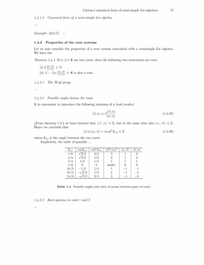
1.4.2.2 Possible angles betwee the roots

It is convenient to introduce the following notation of a hook product

〈β, α〉 ≡ 2(β, α)

(α, α)(1.4.97)

¿From theorem 1.4.1 we have learned that 〈β , α 〉 ∈ Z, but at the same time also 〈α , β 〉 ∈ Z.Hence we conclude that

〈β, α〉〈α, β〉 = 4 cos2 θαβ ∈ Z (1.4.98)

where θαβ is the angle between the two roots.Explicitely, the table of possible ...

θαβ cos θαβ cos2 θαβ |β|2/|α|2 〈α, β〉〈β, α〉π/6

√3/2 3/4 3 1 3

π/4√2/2 1/2 2 1 2

π/3 1/2 1/4 1 1 1π/2 0 0 undet. 0 02π/3 −1/2 1/4 1 −1 −13π/4 −

√2/2 1/2 2 −1 −2

5π/6 −√3/2 3/4 3 −1 −3

Table 1.1. Possible angles and ratio of norms between pairs of roots.

1.4.2.3 Root systems in rank 1 and 2

...


1.4.3 Simple root systems and the Cartan matrix

...

1.4.3.1 Decomposable root systems

...

1.4.3.2 Simple root systems

..

1.4.3.3 The Cartan matrix

The Cartan matrix associated to a simple root system ∆ = {alphai}, i = 1, . . . , r, of a simpleLie algebra of ramk r is defined by

Cij = 〈αi, αj〉 = 2(αi, αj)

(αj , αj). (1.4.99)

According to Eq. (??), there are only the following possibilities

Cii = 2 , ∀i ,

Cij = 0,−1,−2,−3 , ∀i 6= j . (1.4.100)

Notice that the Cartan matrix is in general not symmetric: 〈αi, αj〉 6= 〈αj , αi〉 unless the tworoots have the same length. So the Cartan matrix is symmetric only if all the simple roots havethe same length (in which case the algebra is said to be a simply-laced Lie algebra.

Example For instance, consider the root system B2 of Fig. ??. We have 〈α1, α2〉 = −1 and〈α2, α1〉 = −2, so that the corresponding Cartan matrix is

C =

(

2 −1−2 2

)

. (1.4.101)

Example: the Lie algebra A2 ∼ sl(3,C) ...

Example: the G2 algebra ...

1.4.4 Dynkin diagrams and the classification of simple Lie algebras

Having established that all possible irreducible root systems Φ are uniquely determined (up toisomorphisms) by the Cartan matrix:

Cij =< αi , αj >≡ 2(αi , αj)

(αj , αj)(1.4.102)

we can classify all the complex simple Lie algebras by classifying all possible Cartan matrices.


PSfrag replacements

α1

α1

α2

α2

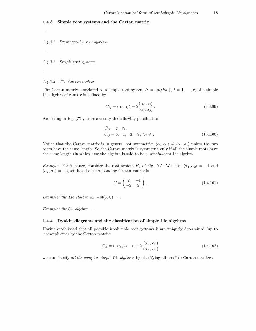
Figure 1.1. The root system G2.

i

α1

i

α2

i

α3

i

α4

. . . i

αr−1

i

α`

Figure 1.2. The simple roots αi are represented by circles

1.4.4.1 Dynkin diagrams

Each Cartan matrix can be given a graphical representation in the following way. To each simpleroot αi we associate a circle © as in fig.1.2 and then we link the i-th circle with the j-th circleby means of a line which is simple, double or triple depending on whether

< αi , αj >< αj , αi >= 4 cos2 θij =

{

123

(1.4.103)

having denoted θij the angle between the two simple roots αi and αj . The corresponding graphis named a Coxeter graph.

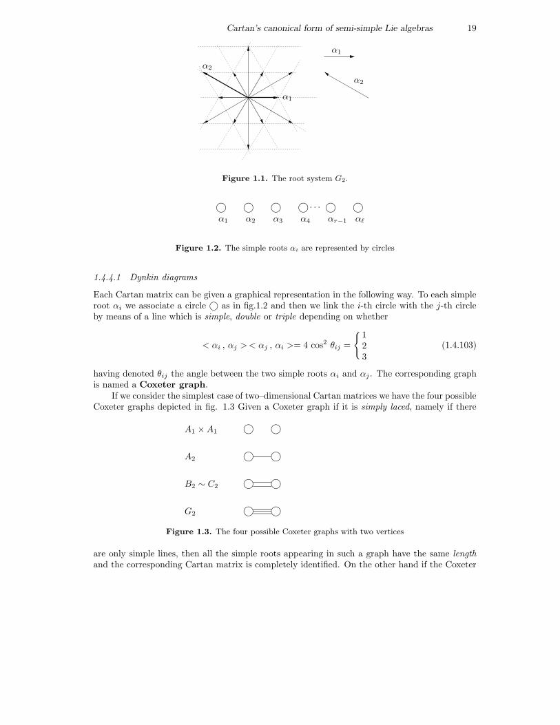
If we consider the simplest case of two–dimensional Cartan matrices we have the four possibleCoxeter graphs depicted in fig. 1.3 Given a Coxeter graph if it is simply laced, namely if there

A1 ×A1i i

A2i i

B2 ∼ C2i i

G2i i

Figure 1.3. The four possible Coxeter graphs with two vertices

are only simple lines, then all the simple roots appearing in such a graph have the same lengthand the corresponding Cartan matrix is completely identified. On the other hand if the Coxeter


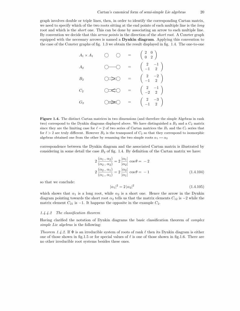
graph involves double or triple lines, then, in order to identify the corresponding Cartan matrix,we need to specify which of the two roots sitting at the end points of each multiple line is the longroot and which is the short one. This can be done by associating an arrow to each multiple line.By convention we decide that this arrow points in the direction of the short root. A Coxeter graphequipped with the necessary arrows is named a Dynkin diagram. Applying this convention tothe case of the Coxeter graphs of fig. 1.3 we obtain the result displayed in fig. 1.4. The one-to-one

A1 ×A1i i =

(

2 00 2

)

A2i i =

(

2 −1−1 2

)

B2i> i =

(

2 −2−1 2

)

C2i< i =

(

2 −1−2 2

)

G2i> i =

(

2 −3−1 2

)

Figure 1.4. The distinct Cartan matrices in two dimensions (and therefore the simple Algebras in rank

two) correspond to the Dynkin diagrams displayed above. We have distinguished a B2 and a C2 matrix

since they are the limiting case for ` = 2 of two series of Cartan matrices the B` and the C` series that

for ` > 2 are truly different. However B2 is the transposed of C2 so that they correspond to isomorphic

algebras obtained one from the other by renaming the two simple roots α1 ↔ α2

correspondence between the Dynkin diagram and the associated Cartan matrix is illustrated byconsidering in some detail the case B2 of fig. 1.4. By definition of the Cartan matrix we have:

2(α1 , α2)

(α2 , α2)= 2|α1|

|α2|cos θ = − 2

2(α2 , α1)

(α1 , α1)= 2|α2|

|α1|cos θ = − 1 (1.4.104)

so that we conclude:|α1|

2 = 2 |α2|2 (1.4.105)

which shows that α1 is a long root, while α2 is a short one. Hence the arrow in the Dynkindiagram pointing towards the short root α2 tells us that the matrix elements C12 is −2 while thematrix element C21 is −1. It happens the opposite in the example C2.

1.4.4.2 The classification theorem

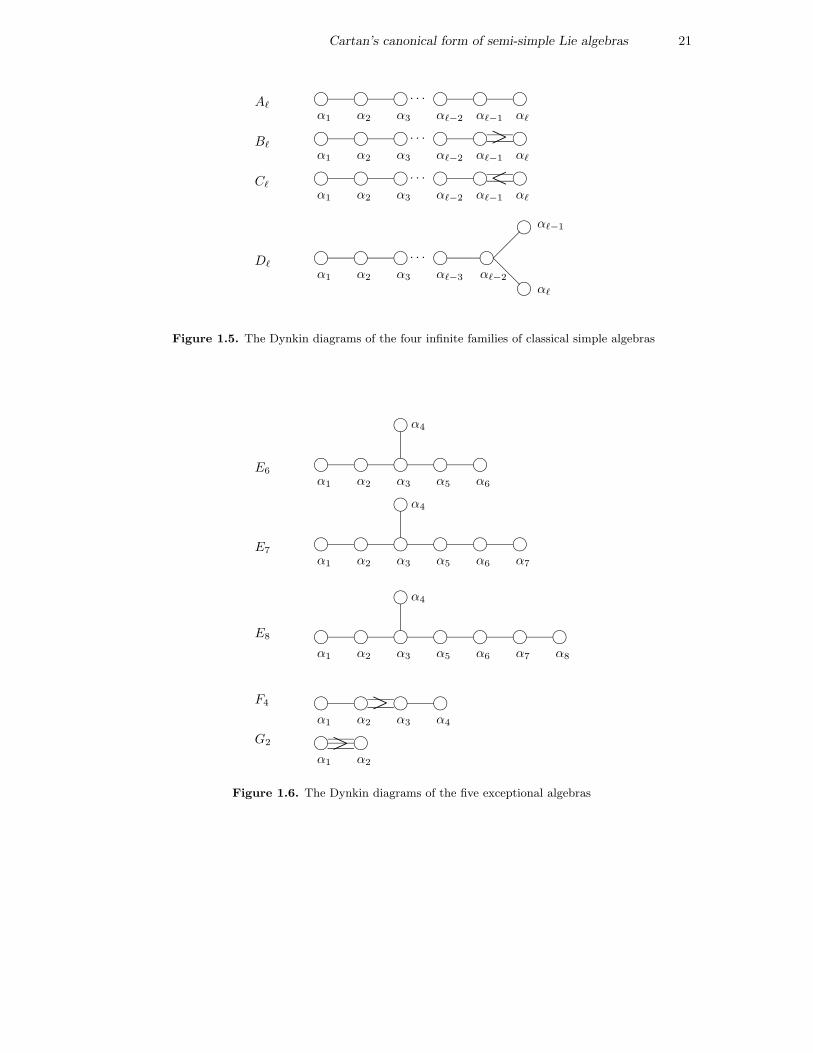
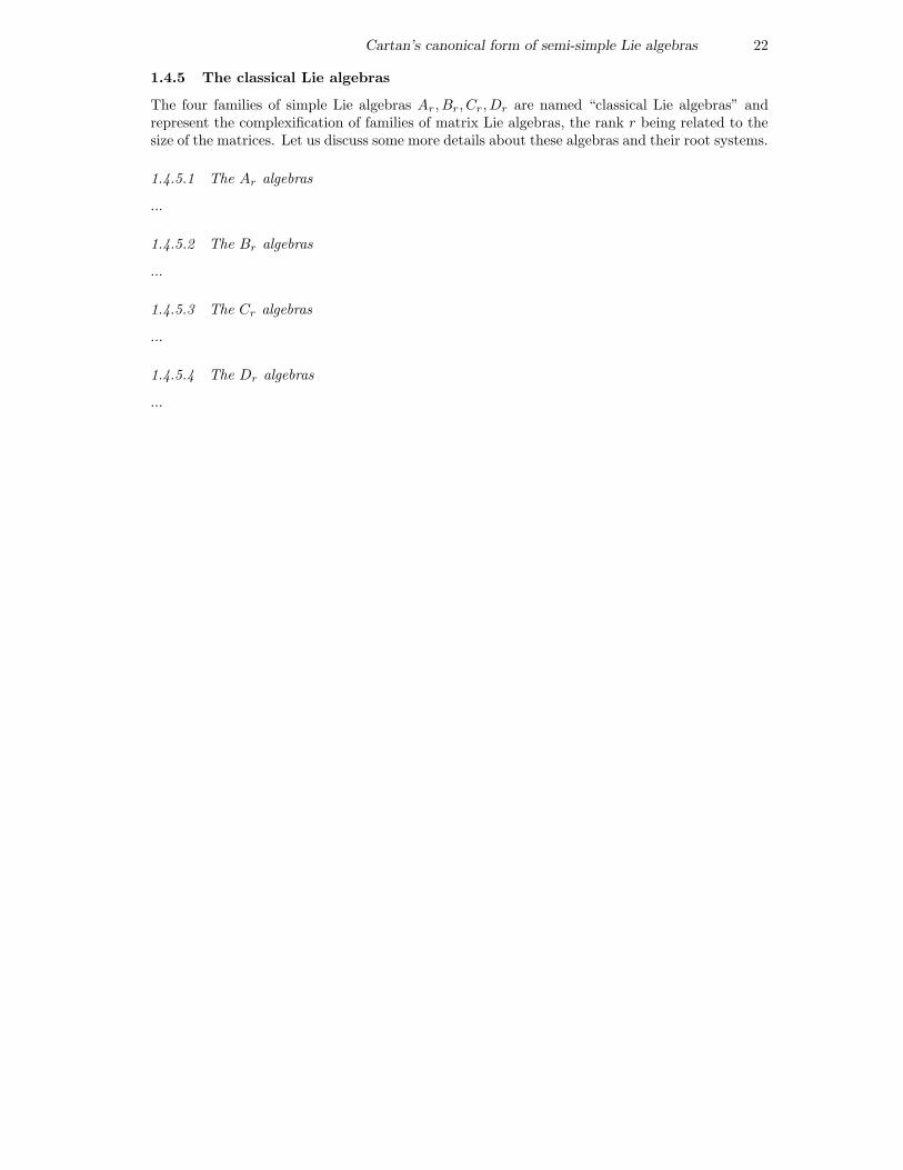
Having clarified the notation of Dynkin diagrams the basic classification theorem of complexsimple Lie algebras is the following:

Theorem 1.4.2. If Φ is an irreducible system of roots of rank ` then its Dynkin diagram is eitherone of those shown in fig.1.5 or for special values of ` is one of those shown in fig.1.6. There areno other irreducible root systems besides these ones.


Aì

α1

i

α2

i

α3

. . . i

α`−2

i

α`−1

i

α`

Bì

α1

i

α2

i

α3

. . . i

α`−2

i

α`−1

> i

α`

Cì

α1

i

α2

i

α3

. . . i

α`−2

i

α`−1

< i

α`

Dì

α1

i

α2

i

α3

. . . i

α`−3

i

α`−2

¡¡

@@

i

i

α`−1

α`

Figure 1.5. The Dynkin diagrams of the four infinite families of classical simple algebras

E6i

α1

i

α2

i

α3

iα4

i

α5

i

α6

E7i

α1

i

α2

i

α3

iα4

i

α5

i

α6

i

α7

E8 i

α1

i

α2

i

α3

iα4

i

α5

i

α6

i

α7

i

α8

F4 i

α1

i

α2

> i

α3

i

α4

G2 i

α1

> i

α2

Figure 1.6. The Dynkin diagrams of the five exceptional algebras


1.4.5 The classical Lie algebras

The four families of simple Lie algebras Ar, Br, Cr, Dr are named “classical Lie algebras” andrepresent the complexification of families of matrix Lie algebras, the rank r being related to thesize of the matrices. Let us discuss some more details about these algebras and their root systems.

1.4.5.1 The Ar algebras

...

1.4.5.2 The Br algebras

...

1.4.5.3 The Cr algebras

...

1.4.5.4 The Dr algebras

...

chapter 1 structure of lie algebraspersonalpages.to.infn.it/~billo/didatt/gruppi/liealgebras.pdf ·...

Documents