chapter 11 dynamic programming - unicampandreani/ms515/capitulo7.pdf · 533 11 dynamic programming...

533

11Dynamic Programming

Dynamic programming is a useful mathematical technique for making a sequence of in-terrelated decisions. It provides a systematic procedure for determining the optimal com-bination of decisions.

In contrast to linear programming, there does not exist a standard mathematical for-mulation of “the” dynamic programming problem. Rather, dynamic programming is a gen-eral type of approach to problem solving, and the particular equations used must be de-veloped to fit each situation. Therefore, a certain degree of ingenuity and insight into thegeneral structure of dynamic programming problems is required to recognize when andhow a problem can be solved by dynamic programming procedures. These abilities canbest be developed by an exposure to a wide variety of dynamic programming applicationsand a study of the characteristics that are common to all these situations. A large numberof illustrative examples are presented for this purpose.

11.1 A PROTOTYPE EXAMPLE FOR DYNAMIC PROGRAMMING

EXAMPLE 1 The Stagecoach Problem

The STAGECOACH PROBLEM is a problem specially constructed1 to illustrate the fea-tures and to introduce the terminology of dynamic programming. It concerns a mythicalfortune seeker in Missouri who decided to go west to join the gold rush in California dur-ing the mid-19th century. The journey would require traveling by stagecoach through un-settled country where there was serious danger of attack by marauders. Although his start-ing point and destination were fixed, he had considerable choice as to which states (orterritories that subsequently became states) to travel through en route. The possible routesare shown in Fig. 11.1, where each state is represented by a circled letter and the direc-tion of travel is always from left to right in the diagram. Thus, four stages (stagecoachruns) were required to travel from his point of embarkation in state A (Missouri) to hisdestination in state J (California).

This fortune seeker was a prudent man who was quite concerned about his safety. Af-ter some thought, he came up with a rather clever way of determining the safest route. Life

1This problem was developed by Professor Harvey M. Wagner while he was at Stanford University.

insurance policies were offered to stagecoach passengers. Because the cost of the policyfor taking any given stagecoach run was based on a careful evaluation of the safety of thatrun, the safest route should be the one with the cheapest total life insurance policy.

The cost for the standard policy on the stagecoach run from state i to state j, whichwill be denoted by cij, is

534 11 DYNAMIC PROGRAMMING

3

4

7 4 6

3 2 4

4 1 5

1 4

6 3

3 3

2 4 3

B C D E F G H I J

A B

C

D

E

F

G

H

I

These costs are also shown in Fig. 11.1.We shall now focus on the question of which route minimizes the total cost of the

policy.

Solving the Problem

First note that the shortsighted approach of selecting the cheapest run offered by each suc-cessive stage need not yield an overall optimal decision. Following this strategy wouldgive the route A � B � F � I � J, at a total cost of 13. However, sacrificing a little onone stage may permit greater savings thereafter. For example, A � D � F is cheaperoverall than A � B � F.

One possible approach to solving this problem is to use trial and error.1 However, thenumber of possible routes is large (18), and having to calculate the total cost for eachroute is not an appealing task.

A C F

D G

B E

I

H

J

2

4

3

64

71

33

2

4

41

53

3

3

6

4

4

FIGURE 11.1The road system and costsfor the stagecoach problem.

1This problem also can be formulated as a shortest-path problem (see Sec. 9.3), where costs here play the roleof distances in the shortest-path problem. The algorithm presented in Sec. 9.3 actually uses the philosophy ofdynamic programming. However, because the present problem has a fixed number of stages, the dynamic pro-gramming approach presented here is even better.

Fortunately, dynamic programming provides a solution with much less effort than ex-haustive enumeration. (The computational savings are enormous for larger versions of thisproblem.) Dynamic programming starts with a small portion of the original problem andfinds the optimal solution for this smaller problem. It then gradually enlarges the prob-lem, finding the current optimal solution from the preceding one, until the original prob-lem is solved in its entirety.

For the stagecoach problem, we start with the smaller problem where the fortuneseeker has nearly completed his journey and has only one more stage (stagecoach run) togo. The obvious optimal solution for this smaller problem is to go from his current state(whatever it is) to his ultimate destination (state J). At each subsequent iteration, the prob-lem is enlarged by increasing by 1 the number of stages left to go to complete the jour-ney. For this enlarged problem, the optimal solution for where to go next from each pos-sible state can be found relatively easily from the results obtained at the preceding iteration.The details involved in implementing this approach follow.

Formulation. Let the decision variables xn (n � 1, 2, 3, 4) be the immediate destina-tion on stage n (the nth stagecoach run to be taken). Thus, the route selected is A �x1 � x2 � x3 � x4, where x4 � J.

Let fn(s, xn) be the total cost of the best overall policy for the remaining stages, giventhat the fortune seeker is in state s, ready to start stage n, and selects xn as the immedi-ate destination. Given s and n, let xn* denote any value of xn (not necessarily unique) thatminimizes fn(s, xn), and let f n* (s) be the corresponding minimum value of fn(s, xn). Thus,

f n*(s) � min fn(s, xn) � fn(s, xn*),xn

where

fn(s, xn) � immediate cost (stage n) � minimum future cost (stages n � 1 onward)� csxn

� f n*�1(xn).

The value of csxnis given by the preceding tables for cij by setting i � s (the current state)

and j � xn (the immediate destination). Because the ultimate destination (state J) is reachedat the end of stage 4, f 5* ( J) � 0.

The objective is to find f 1* (A) and the corresponding route. Dynamic programmingfinds it by successively finding f 4*(s), f 3*(s), f 2*(s), for each of the possible states s andthen using f 2*(s) to solve for f 1*(A).1

Solution Procedure. When the fortune seeker has only one more stage to go (n � 4),his route thereafter is determined entirely by his current state s (either H or I) and his fi-nal destination x4 � J, so the route for this final stagecoach run is s � J. Therefore, sincef 4*(s) � f4(s, J) � cs,J, the immediate solution to the n � 4 problem is

11.1 A PROTOTYPE EXAMPLE FOR DYNAMIC PROGRAMMING 535

n � 4: s f 4*(s) x4*

H 3 JI 4 J

1Because this procedure involves moving backward stage by stage, some writers also count n backward to denotethe number of remaining stages to the destination. We use the more natural forward counting for greater simplicity.

When the fortune seeker has two more stages to go (n � 3), the solution procedurerequires a few calculations. For example, suppose that the fortune seeker is in state F.Then, as depicted below, he must next go to either state H or I at an immediate cost ofcF,H � 6 or cF,I � 3, respectively. If he chooses state H, the minimum additional cost af-ter he reaches there is given in the preceding table as f 4*(H) � 3, as shown above the Hnode in the diagram. Therefore, the total cost for this decision is 6 � 3 � 9. If he choosesstate I instead, the total cost is 3 � 4 � 7, which is smaller. Therefore, the optimal choiceis this latter one, x3* � I, because it gives the minimum cost f 3*(F) � 7.


F

H

I

6

3

4

3

Similar calculations need to be made when you start from the other two possible statess � E and s � G with two stages to go. Try it, proceeding both graphically (Fig. 11.1)and algebraically [combining cij and f 4*(s) values], to verify the following complete re-sults for the n � 3 problem.

f3(s, x3) � csx3� f 4*(x3)

x3

n � 3: s H I f 3*(s) x3*

E 4 8 4 HF 9 7 7 IG 6 7 6 H

The solution for the second-stage problem (n � 2), where there are three stages togo, is obtained in a similar fashion. In this case, f2(s, x2) � csx2

� f 3*(x2). For example,suppose that the fortune seeker is in state C, as depicted below.

C

E

G

3

2

4

F

7

6

4

He must next go to state E, F, or G at an immediate cost of cC,E � 3, cC,F � 2, or cC,G � 4, respectively. After getting there, the minimum additional cost for stage 3 to theend is given by the n � 3 table as f 3*(E) � 4, f 3*(F) � 7, or f 3*(G) � 6, respectively, asshown above the E and F nodes and below the G node in the preceding diagram. The re-sulting calculations for the three alternatives are summarized below.

x2 � E: f2(C, E) � cC,E � f 3*(E) � 3 � 4 � 7.x2 � F: f2(C, F) � cC,F � f 3*(F) � 2 � 7 � 9.x2 � G: f2(C, G) � cC,G � f 3*(G) � 4 � 6 � 10.

The minimum of these three numbers is 7, so the minimum total cost from state C to theend is f 2*(C ) � 7, and the immediate destination should be x2* � E.

Making similar calculations when you start from state B or D (try it) yields the fol-lowing results for the n � 2 problem:

11.1 A PROTOTYPE EXAMPLE FOR DYNAMIC PROGRAMMING 537

f2(s, x2) � csx2� f 3*(x2)

x2

n � 2: s E F G f 2*(s) x2*

B 11 11 12 11 E or FC 7 9 10 7 ED 8 8 11 8 E or F

In the first and third rows of this table, note that E and F tie as the minimizing value ofx2, so the immediate destination from either state B or D should be x2* � E or F.

Moving to the first-stage problem (n � 1), with all four stages to go, we see that thecalculations are similar to those just shown for the second-stage problem (n � 2), exceptnow there is just one possible starting state s � A, as depicted below.

These calculations are summarized next for the three alternatives for the immediate des-tination:

x1 � B: f1(A, B) � cA,B � f 2*(B) � 2 � 11 � 13.x1 � C: f1(A, C) � cA,C � f 2*(C ) � 4 � 7 � 11.x1 � D: f1(A, D) � cA,D � f 2*(D) � 3 � 8 � 11.

A

B

D

2

4

11

C

7

8

3

Since 11 is the minimum, f 1*(A) � 11 and x1* � C or D, as shown in the following table.


f1(s, x1) � csx1� f 2*(x1)

x1

n � 1: s B C D f 1*(s) x1*

A 13 11 11 11 C or D

An optimal solution for the entire problem can now be identified from the four ta-bles. Results for the n � 1 problem indicate that the fortune seeker should go initially toeither state C or state D. Suppose that he chooses x1* � C. For n � 2, the result for s � Cis x2* � E. This result leads to the n � 3 problem, which gives x3* � H for s � E, and then � 4 problem yields x4* � J for s � H. Hence, one optimal route is A � C � E �H � J. Choosing x1* � D leads to the other two optimal routes A � D � E � H � Jand A � D � F � I � J. They all yield a total cost of f 1*(A) � 11.

These results of the dynamic programming analysis also are summarized in Fig. 11.2.Note how the two arrows for stage 1 come from the first and last columns of the n � 1table and the resulting cost comes from the next-to-last column. Each of the other arrows(and the resulting cost) comes from one row in one of the other tables in just the same way.

You will see in the next section that the special terms describing the particular con-text of this problem—stage, state, and policy—actually are part of the general terminol-ogy of dynamic programming with an analogous interpretation in other contexts.

G

I

T4

3

4

71

33

4

1 3

34

CA F

E

H

D

B

11

11 4

3

77

8 6

4

1 2 3 4Stage:

State:

FIGURE 11.2Graphical display of thedynamic programmingsolution of the stagecoachproblem. Each arrow showsan optimal policy decision(the best immediatedestination) from that state,where the number by thestate is the resulting costfrom there to the end.Following the boldfacearrows from A to T gives thethree optimal solutions (thethree routes giving theminimum total cost of 11).

The stagecoach problem is a literal prototype of dynamic programming problems. In fact,this example was purposely designed to provide a literal physical interpretation of therather abstract structure of such problems. Therefore, one way to recognize a situation

11.2 CHARACTERISTICS OF DYNAMIC PROGRAMMING PROBLEMS

that can be formulated as a dynamic programming problem is to notice that its basic struc-ture is analogous to the stagecoach problem.

These basic features that characterize dynamic programming problems are presentedand discussed here.

1. The problem can be divided into stages, with a policy decision required at each stage.The stagecoach problem was literally divided into its four stages (stagecoaches)

that correspond to the four legs of the journey. The policy decision at each stage waswhich life insurance policy to choose (i.e., which destination to select for the next stage-coach ride). Similarly, other dynamic programming problems require making a sequenceof interrelated decisions, where each decision corresponds to one stage of the problem.

2. Each stage has a number of states associated with the beginning of that stage.The states associated with each stage in the stagecoach problem were the states

(or territories) in which the fortune seeker could be located when embarking on thatparticular leg of the journey. In general, the states are the various possible conditionsin which the system might be at that stage of the problem. The number of states maybe either finite (as in the stagecoach problem) or infinite (as in some subsequent ex-amples).

3. The effect of the policy decision at each stage is to transform the current state to astate associated with the beginning of the next stage (possibly according to a proba-bility distribution).

The fortune seeker’s decision as to his next destination led him from his currentstate to the next state on his journey. This procedure suggests that dynamic program-ming problems can be interpreted in terms of the networks described in Chap. 9. Eachnode would correspond to a state. The network would consist of columns of nodes,with each column corresponding to a stage, so that the flow from a node can go onlyto a node in the next column to the right. The links from a node to nodes in the nextcolumn correspond to the possible policy decisions on which state to go to next. Thevalue assigned to each link usually can be interpreted as the immediate contribution tothe objective function from making that policy decision. In most cases, the objectivecorresponds to finding either the shortest or the longest path through the network.

4. The solution procedure is designed to find an optimal policy for the overall problem,i.e., a prescription of the optimal policy decision at each stage for each of the possi-ble states.

For the stagecoach problem, the solution procedure constructed a table for eachstage (n) that prescribed the optimal decision (xn*) for each possible state (s). Thus, inaddition to identifying three optimal solutions (optimal routes) for the overall problem,the results show the fortune seeker how he should proceed if he gets detoured to a statethat is not on an optimal route. For any problem, dynamic programming provides thiskind of policy prescription of what to do under every possible circumstance (which iswhy the actual decision made upon reaching a particular state at a given stage is re-ferred to as a policy decision). Providing this additional information beyond simplyspecifying an optimal solution (optimal sequence of decisions) can be helpful in a va-riety of ways, including sensitivity analysis.

5. Given the current state, an optimal policy for the remaining stages is independent ofthe policy decisions adopted in previous stages. Therefore, the optimal immediate de-

11.2 CHARACTERISTICS OF DYNAMIC PROGRAMMING PROBLEMS 539

cision depends on only the current state and not on how you got there. This is the prin-ciple of optimality for dynamic programming.

Given the state in which the fortune seeker is currently located, the optimal lifeinsurance policy (and its associated route) from this point onward is independent ofhow he got there. For dynamic programming problems in general, knowledge of thecurrent state of the system conveys all the information about its previous behavior nec-essary for determining the optimal policy henceforth. (This property is the Markovianproperty, discussed in Sec. 16.2.) Any problem lacking this property cannot be for-mulated as a dynamic programming problem.

6. The solution procedure begins by finding the optimal policy for the last stage.The optimal policy for the last stage prescribes the optimal policy decision for

each of the possible states at that stage. The solution of this one-stage problem is usu-ally trivial, as it was for the stagecoach problem.

7. A recursive relationship that identifies the optimal policy for stage n, given the opti-mal policy for stage n � 1, is available.

For the stagecoach problem, this recursive relationship was

f n*(s) � minxn

{csxn� f *n�1(xn)}.

Therefore, finding the optimal policy decision when you start in state s at stage n re-quires finding the minimizing value of xn. For this particular problem, the correspondingminimum cost is achieved by using this value of xn and then following the optimal pol-icy when you start in state xn at stage n � 1.

The precise form of the recursive relationship differs somewhat among dynamicprogramming problems. However, notation analogous to that introduced in the pre-ceding section will continue to be used here, as summarized below.

N � number of stages.

n � label for current stage (n � 1, 2, . . . , N ).

sn � current state for stage n.

xn � decision variable for stage n.

xn* � optimal value of xn (given sn).

fn(sn, xn) � contribution of stages n, n � 1, . . . , N to objective function if system startsin state sn at stage n, immediate decision is xn, and optimal decisions aremade thereafter.

f n*(sn) � fn(sn, xn*).

The recursive relationship will always be of the form

f n*(sn) � max { fn(sn, xn)} or f n*(sn) � min {fn(sn, xn)},xn xn

where fn(sn, xn) would be written in terms of sn, xn, f *n�1(sn�1), and probably somemeasure of the immediate contribution of xn to the objective function. It is the inclu-sion of f *n�1(sn�1) on the right-hand side, so that f *n(sn) is defined in terms of f *n�1(sn�1),that makes the expression for f *n(sn) a recursive relationship.

The recursive relationship keeps recurring as we move backward stage by stage.When the current stage number n is decreased by 1, the new f *n(sn) function is derived


by using the f *n�1(sn�1) function that was just derived during the preceding iteration,and then this process keeps repeating. This property is emphasized in the next (and fi-nal) characteristic of dynamic programming.

8. When we use this recursive relationship, the solution procedure starts at the end andmoves backward stage by stage—each time finding the optimal policy for that stage—until it finds the optimal policy starting at the initial stage. This optimal policy imme-diately yields an optimal solution for the entire problem, namely, x1* for the initial states1, then x2* for the resulting state s2, then x3* for the resulting state s3, and so forth tox*N for the resulting stage sN.

This backward movement was demonstrated by the stagecoach problem, where theoptimal policy was found successively beginning in each state at stages 4, 3, 2, and 1,respectively.1 For all dynamic programming problems, a table such as the followingwould be obtained for each stage (n � N, N � 1, . . . , 1).

11.3 DETERMINISTIC DYNAMIC PROGRAMMING 541

fn(sn, xn)xn

sn f n*(sn) xn*

When this table is finally obtained for the initial stage (n � 1), the problem of interestis solved. Because the initial state is known, the initial decision is specified by x1* in thistable. The optimal value of the other decision variables is then specified by the other ta-bles in turn according to the state of the system that results from the preceding decisions.

This section further elaborates upon the dynamic programming approach to deterministicproblems, where the state at the next stage is completely determined by the state and pol-icy decision at the current stage. The probabilistic case, where there is a probability dis-tribution for what the next state will be, is discussed in the next section.

Deterministic dynamic programming can be described diagrammatically as shown inFig. 11.3. Thus, at stage n the process will be in some state sn. Making policy decisionxn then moves the process to some state sn�1 at stage n � 1. The contribution thereafterto the objective function under an optimal policy has been previously calculated to bef *n�1(sn�1). The policy decision xn also makes some contribution to the objective func-tion. Combining these two quantities in an appropriate way provides fn(sn, xn), the con-tribution of stages n onward to the objective function. Optimizing with respect to xn thengives f n*(sn) � fn(sn, xn*). After xn* and f n*(sn) are found for each possible value of sn, thesolution procedure is ready to move back one stage.

One way of categorizing deterministic dynamic programming problems is by the formof the objective function. For example, the objective might be to minimize the sum of thecontributions from the individual stages (as for the stagecoach problem), or to maximize

11.3 DETERMINISTIC DYNAMIC PROGRAMMING

1Actually, for this problem the solution procedure can move either backward or forward. However, for manyproblems (especially when the stages correspond to time periods), the solution procedure must move backward.

such a sum, or to minimize a product of such terms, and so on. Another categorization isin terms of the nature of the set of states for the respective stages. In particular, states sn

might be representable by a discrete state variable (as for the stagecoach problem) or bya continuous state variable, or perhaps a state vector (more than one variable) is required.

Several examples are presented to illustrate these various possibilities. More impor-tantly, they illustrate that these apparently major differences are actually quite inconse-quential (except in terms of computational difficulty) because the underlying basic struc-ture shown in Fig. 11.3 always remains the same.

The first new example arises in a much different context from the stagecoach prob-lem, but it has the same mathematical formulation except that the objective is to maxi-mize rather than minimize a sum.


State:

Stagen

Stagen � 1

sn sn � 1Contribution

of xnfn(sn, xn) f *n � 1(sn � 1)

xn

Value:

FIGURE 11.3The basic structure fordeterministic dynamicprogramming.

TABLE 11.1 Data for the World Health Council problem

Thousands of AdditionalPerson-Years of Life

CountryMedicalTeams 1 2 3

0 0 0 01 45 20 502 70 45 703 90 75 804 105 110 1005 120 150 130

EXAMPLE 2 Distributing Medical Teams to Countries

The WORLD HEALTH COUNCIL is devoted to improving health care in the underde-veloped countries of the world. It now has five medical teams available to allocate amongthree such countries to improve their medical care, health education, and training pro-grams. Therefore, the council needs to determine how many teams (if any) to allocate toeach of these countries to maximize the total effectiveness of the five teams. The teamsmust be kept intact, so the number allocated to each country must be an integer.

The measure of performance being used is additional person-years of life. (For a par-ticular country, this measure equals the increased life expectancy in years times the coun-try’s population.) Table 11.1 gives the estimated additional person-years of life (in multi-ples of 1,000) for each country for each possible allocation of medical teams.

Which allocation maximizes the measure of performance?

Formulation. This problem requires making three interrelated decisions, namely, howmany medical teams to allocate to each of the three countries. Therefore, even thoughthere is no fixed sequence, these three countries can be considered as the three stages ina dynamic programming formulation. The decision variables xn (n � 1, 2, 3) are the num-ber of teams to allocate to stage (country) n.

The identification of the states may not be readily apparent. To determine the states,we ask questions such as the following. What is it that changes from one stage to the next?Given that the decisions have been made at the previous stages, how can the status of thesituation at the current stage be described? What information about the current state ofaffairs is necessary to determine the optimal policy hereafter? On these bases, an appro-priate choice for the “state of the system” is

sn � number of medical teams still available for allocation to remaining countries(n, . . . , 3).

Thus, at stage 1 (country 1), where all three countries remain under consideration for al-locations, s1 � 5. However, at stage 2 or 3 (country 2 or 3), sn is just 5 minus the num-ber of teams allocated at preceding stages, so that the sequence of states is

s1 � 5, s2 � 5 � x1, s3 � s2 � x2.

With the dynamic programming procedure of solving backward stage by stage, when weare solving at stage 2 or 3, we shall not yet have solved for the allocations at the preced-ing stages. Therefore, we shall consider every possible state we could be in at stage 2 or3, namely, sn � 0, 1, 2, 3, 4, or 5.

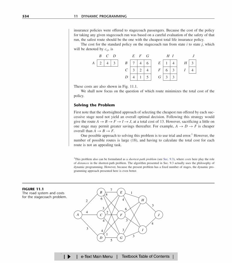
Figure 11.4 shows the states to be considered at each stage. The links (line segments)show the possible transitions in states from one stage to the next from making a feasibleallocation of medical teams to the country involved. The numbers shown next to the linksare the corresponding contributions to the measure of performance, where these numberscome from Table 11.1. From the perspective of this figure, the overall problem is to findthe path from the initial state 5 (beginning stage 1) to the final state 0 (after stage 3) thatmaximizes the sum of the numbers along the path.

To state the overall problem mathematically, let pi(xi) be the measure of performancefrom allocating xi medical teams to country i, as given in Table 11.1. Thus, the objectiveis to choose x1, x2, x3 so as to

Maximize �3

i�1pi(xi),

subject to

�3

i�1xi � 5,

and

xi are nonnegative integers.

Using the notation presented in Sec. 11.2, we see that fn(sn, xn) is

fn(sn, xn) � pn(xn) � max �3

i�n�1pi(xi),


where the maximum is taken over xn�1, . . . , x3 such that

�3

i�n

xi � sn

and the xi are nonnegative integers, for n � 1, 2, 3. In addition,

f n*(sn) � max fn(sn, xn)xn�0,1, . . . , sn

Therefore,

fn(sn, xn) � pn(xn) � f *n�1(sn � xn)

(with f 4* defined to be zero). These basic relationships are summarized in Fig. 11.5.


Stage:

State:

1 2 3

0 0

120

20150

50

700

105

45

20110

80

100

130

0

75

45 20

4575

900

110

7520

70

0 0

20

0

45

45

0 0 0

1 1

2 2

33

44

555

FIGURE 11.4Graphical display of theWorld Health Councilproblem, showing thepossible states at each stage,the possible transitions instates, and the correspondingcontributions to the measureof performance.

Consequently, the recursive relationship relating functions f 1*, f 2*, and f 3* for this prob-lem is

f n*(sn) � max {pn(xn) � f *n�1(sn � xn)}, for n � 1, 2.xn�0,1, . . . , sn

For the last stage (n � 3),

f 3*(s3) � max p3(x3).x3�0,1, . . . , s3

The resulting dynamic programming calculations are given next.

Solution Procedure. Beginning with the last stage (n � 3), we note that the values ofp3(x3) are given in the last column of Table 11.1 and these values keep increasing as wemove down the column. Therefore, with s3 medical teams still available for allocation tocountry 3, the maximum of p3(x3) is automatically achieved by allocating all s3 teams; sox3* � s3 and f 3*(s3) � p3(s3), as shown in the following table.


sn sn � xn

Stagen � 1

Stagen

State:

Value: fn(sn, xn) pn(xn)� pn(xn) � f *

n � 1(sn � xn)

f *n � 1(sn � xn)

xn

n � 3: s3 f 3*(s3) x3*

0 0 01 50 12 70 23 80 34 100 45 130 5

We now move backward to start from the next-to-last stage (n � 2). Here, finding x2* requires calculating and comparing f2(s2, x2) for the alternative values of x2, namely,x2 � 0, 1, . . . , s2. To illustrate, we depict this situation when s2 � 2 graphically:

FIGURE 11.5The basic structure for theWorld Health Councilproblem.

2

0

2

45

20

0

1

50

70

0

State:

This diagram corresponds to Fig. 11.5 except that all three possible states at stage 3 areshown. Thus, if x2 � 0, the resulting state at stage 3 will be s2 � x2 � 2 � 0 � 2, whereasx2 � 1 leads to state 1 and x2 � 2 leads to state 0. The corresponding values of p2(x2)from the country 2 column of Table 11.1 are shown along the links, and the values off 3*(s2 � x2) from the n � 3 table are given next to the stage 3 nodes. The required calcu-lations for this case of s2 � 2 are summarized below.

Formula: f2(2, x2) � p2(x2) � f 3*(2 � x2).p2(x2) is given in the country 2 column of Table 11.1.f 3*(2 � x2) is given in the n � 3 table (bottom of preceding page).

x2 � 0: f2(2, 0) � p2(0) � f 3*(2) � 0 � 70 � 70.x2 � 1: f2(2, 1) � p2(1) � f 3*(1) � 20 � 50 � 70.x2 � 2: f2(2, 2) � p2(2) � f 3*(0) � 45 � 0 � 45.

Because the objective is maximization, x2* � 0 or 1 with f 2*(2) � 70.Proceeding in a similar way with the other possible values of s2 (try it) yields the fol-

lowing table.


f2(s2, x2) � p2(x2) � f 3*(s2 � x2)x2

n � 2: s2 0 1 2 3 4 5 f 2*(s2) x2*

0 0 0 0 or 11 50 20 50 0 or 12 70 70 45 70 0 or 13 80 90 95 75 95 2 or 14 100 100 115 125 110 125 3 or 15 130 120 125 145 160 150 160 4 or 1

We now are ready to move backward to solve the original problem where we are start-ing from stage 1 (n � 1). In this case, the only state to be considered is the starting stateof s1 � 5, as depicted below.

5

0

5

120

45

0

4

125

160

0

State:

•••

Since allocating x1 medical teams to country 1 leads to a state of 5 � x1 at stage 2, achoice of x1 � 0 leads to the bottom node on the right, x � 1 leads to the next node up,and so forth up to the top node with x1 � 5. The corresponding p1(x1) values from Table

11.1 are shown next to the links. The numbers next to the nodes are obtained from thef 2*(s2) column of the n � 2 table. As with n � 2, the calculation needed for each alterna-tive value of the decision variable involves adding the corresponding link value and nodevalue, as summarized below.

Formula: f1(5, x1) � p1(x1) � f 2*(5 � x1).p1(x1) is given in the country 1 column of Table 11.1.f 2*(5 � x1) is given in the n � 2 table.

x1 � 0: f1(5, 0) � p1(0) � f 2*(5) � 0 � 160 � 160.x1 � 1: f1(5, 1) � p1(1) � f 2*(4) � 45 � 125 � 170.

�

x1 � 5: f1(5, 5) � p1(5) � f 2*(0) � 120 � 0 � 120.

The similar calculations for x1 � 2, 3, 4 (try it) verify that x1* � 1 with f 1*(5) � 170, asshown in the following table.


f1(s1, x1) � p1(x1) � f 2*(s1 � x1)x2

n � 1: s1 0 1 2 3 4 5 f 1*(s1) x1*

5 160 170 165 160 155 120 170 1

Thus, the optimal solution has x1* � 1, which makes s2 � 5 � 1 � 4, so x2* � 3, whichmakes s3 � 4 � 3 � 1, so x3* � 1. Since f 1*(5) � 170, this (1, 3, 1) allocation of medicalteams to the three countries will yield an estimated total of 170,000 additional person-years of life, which is at least 5,000 more than for any other allocation.

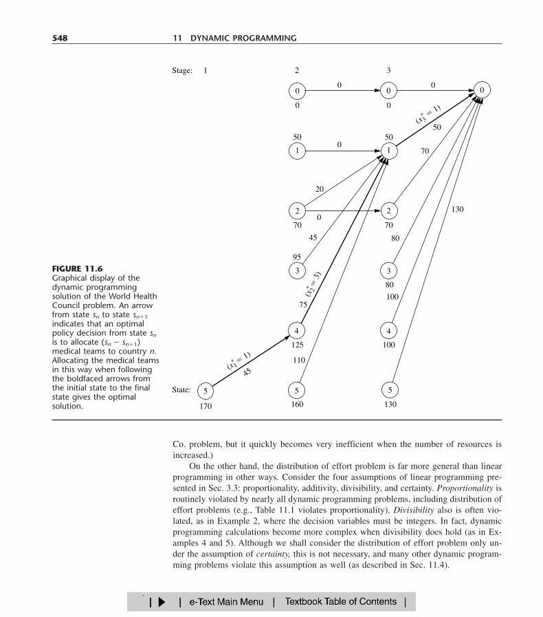
These results of the dynamic programming analysis also are summarized in Fig. 11.6.

A Prevalent Problem Type—The Distribution of Effort Problem

The preceding example illustrates a particularly common type of dynamic programmingproblem called the distribution of effort problem. For this type of problem, there is justone kind of resource that is to be allocated to a number of activities. The objective is todetermine how to distribute the effort (the resource) among the activities most effectively.For the World Health Council example, the resource involved is the medical teams, andthe three activities are the health care work in the three countries.

Assumptions. This interpretation of allocating resources to activities should ring a bellfor you, because it is the typical interpretation for linear programming problems given atthe beginning of Chap. 3. However, there also are some key differences between the dis-tribution of effort problem and linear programming that help illuminate the general dis-tinctions between dynamic programming and other areas of mathematical programming.

One key difference is that the distribution of effort problem involves only one re-source (one functional constraint), whereas linear programming can deal with thousandsof resources. (In principle, dynamic programming can handle slightly more than one re-source, as we shall illustrate in Example 5 by solving the three-resource Wyndor Glass

Co. problem, but it quickly becomes very inefficient when the number of resources isincreased.)

On the other hand, the distribution of effort problem is far more general than linearprogramming in other ways. Consider the four assumptions of linear programming pre-sented in Sec. 3.3: proportionality, additivity, divisibility, and certainty. Proportionality isroutinely violated by nearly all dynamic programming problems, including distribution ofeffort problems (e.g., Table 11.1 violates proportionality). Divisibility also is often vio-lated, as in Example 2, where the decision variables must be integers. In fact, dynamicprogramming calculations become more complex when divisibility does hold (as in Ex-amples 4 and 5). Although we shall consider the distribution of effort problem only un-der the assumption of certainty, this is not necessary, and many other dynamic program-ming problems violate this assumption as well (as described in Sec. 11.4).


State:

2 3

0

1

0 0

0

50 500

0 0

20

70 70

95

80

0

(x 3* �

1)

50

70

2

80

100

100

5

130

130

4

5

(x 1* �

1)

45

170 160

125

110

75(x

2* � 3

)

45

5

2

3 3

1

0

Stage: 1

4

FIGURE 11.6Graphical display of thedynamic programmingsolution of the World HealthCouncil problem. An arrowfrom state sn to state sn�1indicates that an optimalpolicy decision from state snis to allocate (sn � sn�1)medical teams to country n.Allocating the medical teamsin this way when followingthe boldfaced arrows fromthe initial state to the finalstate gives the optimalsolution.

Of the four assumptions of linear programming, the only one needed by the distrib-ution of effort problem (or other dynamic programming problems) is additivity (or its ana-log for functions involving a product of terms). This assumption is needed to satisfy theprinciple of optimality for dynamic programming (characteristic 5 in Sec. 11.2).

Formulation. Because they always involve allocating one kind of resource to a num-ber of activities, distribution of effort problems always have the following dynamic pro-gramming formulation (where the ordering of the activities is arbitrary):

Stage n � activity n (n � 1, 2, . . . , N ).xn � amount of resource allocated to activity n.

State sn � amount of resource still available for allocation to remaining activities(n, . . . , N ).

The reason for defining state sn in this way is that the amount of the resource still avail-able for allocation is precisely the information about the current state of affairs (enteringstage n) that is needed for making the allocation decisions for the remaining activities.

When the system starts at stage n in state sn, the choice of xn results in the next stateat stage n � 1 being sn�1 � sn � xn, as depicted below:1


sn sn � xnxn

n � 1n

State:

Stage:

1This statement assumes that xn and sn are expressed in the same units. If it is more convenient to define xn assome other quantity such that the amount of the resource allocated to activity n is anxn, then sn�1 � sn � anxn.

Note how the structure of this diagram corresponds to the one shown in Fig. 11.5 for theWorld Health Council example of a distribution of effort problem. What will differ fromone such example to the next is the rest of what is shown in Fig. 11.5, namely, the rela-tionship between fn(sn, xn) and f *n�1(sn � xn), and then the resulting recursive relationshipbetween the f n* and f *n�1 functions. These relationships depend on the particular objectivefunction for the overall problem.

The structure of the next example is similar to the one for the World Health Councilbecause it, too, is a distribution of effort problem. However, its recursive relationship dif-fers in that its objective is to minimize a product of terms for the respective stages.

At first glance, this example may appear not to be a deterministic dynamic pro-gramming problem because probabilities are involved. However, it does indeed fit our def-inition because the state at the next stage is completely determined by the state and pol-icy decision at the current stage.

EXAMPLE 3 Distributing Scientists to Research Teams

A government space project is conducting research on a certain engineering problem thatmust be solved before people can fly safely to Mars. Three research teams are currentlytrying three different approaches for solving this problem. The estimate has been madethat, under present circumstances, the probability that the respective teams—call them 1,

2, and 3—will not succeed is 0.40, 0.60, and 0.80, respectively. Thus, the current proba-bility that all three teams will fail is (0.40)(0.60)(0.80) � 0.192. Because the objective isto minimize the probability of failure, two more top scientists have been assigned to theproject.

Table 11.2 gives the estimated probability that the respective teams will fail when 0,1, or 2 additional scientists are added to that team. Only integer numbers of scientists areconsidered because each new scientist will need to devote full attention to one team. Theproblem is to determine how to allocate the two additional scientists to minimize the prob-ability that all three teams will fail.

Formulation. Because both Examples 2 and 3 are distribution of effort problems, theirunderlying structure is actually very similar. In this case, scientists replace medical teamsas the kind of resource involved, and research teams replace countries as the activities.Therefore, instead of medical teams being allocated to countries, scientists are being al-located to research teams. The only basic difference between the two problems is in theirobjective functions.

With so few scientists and teams involved, this problem could be solved very easilyby a process of exhaustive enumeration. However, the dynamic programming solution ispresented for illustrative purposes.

In this case, stage n (n � 1, 2, 3) corresponds to research team n, and the state sn is thenumber of new scientists still available for allocation to the remaining teams. The decisionvariables xn (n � 1, 2, 3) are the number of additional scientists allocated to team n.

Let pi(xi) denote the probability of failure for team i if it is assigned xi additional sci-entists, as given by Table 11.2. If we let � denote multiplication, the government’s ob-jective is to choose x1, x2, x3 so as to

Minimize �3

i�1pi(xi) � p1(x1)p2(x2)p3(x3),

subject to

�3

i�1xi � 2


TABLE 11.2 Data for the Government Space Project problem

Probability of Failure

TeamNew

Scientists 1 2 3

0 0.40 0.60 0.801 0.20 0.40 0.502 0.15 0.20 0.30

and

xi are nonnegative integers.

Consequently, fn(sn, xn) for this problem is

fn(sn, xn) � pn(xn) � min �3

i�n�1pi(xi),

where the minimum is taken over xn�1, . . . , x3 such that

�3

i�n

xi � sn

and

xi are nonnegative integers,

for n � 1, 2, 3. Thus,

f n*(sn) � min fn(sn, xn),xn�0,1, . . . , sn

where

fn(sn, xn) � pn(xn) � f *n�1(sn � xn)

(with f 4* defined to be 1). Figure 11.7 summarizes these basic relationships.Thus, the recursive relationship relating the f 1*, f 2*, and f 3* functions in this case is

f n*(sn) � min {pn(xn) � f *n�1(sn � xn)}, for n � 1, 2,xn�0,1, . . . , sn

and, when n � 3,

f 3*(s3) � min p3(x3).x3 � 0,1, . . . , s3

Solution Procedure. The resulting dynamic programming calculations are as follows:


sn sn � xn

Stagen � 1

Stagen

State:

Value: fn(sn, xn) pn(xn)� pn(xn) � f *

n � 1(sn � xn)

f *n � 1(sn � xn)

xn

FIGURE 11.7The basic structure for thegovernment space projectproblem.

n � 3: s3 f 3*(s3) x3*

0 0.80 01 0.50 12 0.30 2

Therefore, the optimal solution must have x1* � 1, which makes s2 � 2 � 1 � 1, so thatx2* � 0, which makes s3 � 1 � 0 � 1, so that x3* � 1. Thus, teams 1 and 3 should eachreceive one additional scientist. The new probability that all three teams will fail wouldthen be 0.060.

All the examples thus far have had a discrete state variable sn at each stage. Fur-thermore, they all have been reversible in the sense that the solution procedure actuallycould have moved either backward or forward stage by stage. (The latter alternativeamounts to renumbering the stages in reverse order and then applying the procedure inthe standard way.) This reversibility is a general characteristic of distribution of effortproblems such as Examples 2 and 3, since the activities (stages) can be ordered in anydesired manner.

The next example is different in both respects. Rather than being restricted to inte-ger values, its state variable sn at stage n is a continuous variable that can take on anyvalue over certain intervals. Since sn now has an infinite number of values, it is no longerpossible to consider each of its feasible values individually. Rather, the solution for f n*(sn)and xn* must be expressed as functions of sn. Furthermore, this example is not reversiblebecause its stages correspond to time periods, so the solution procedure must proceedbackward.


f2(s2, x2) � p2(x2) � f 3*(s2 � x2)x2

n � 2: s2 0 1 2 f 2*(s2) x2*

0 0.48 0.48 01 0.30 0.32 0.30 02 0.18 0.20 0.16 0.16 2

f1(s1, x1) � p1(x1) � f 2*(s1 � x1)x1

n � 1: s1 0 1 2 f 1*(s1) x1*

2 0.064 0.060 0.072 0.060 1

EXAMPLE 4 Scheduling Employment Levels

The workload for the LOCAL JOB SHOP is subject to considerable seasonal fluctuation.However, machine operators are difficult to hire and costly to train, so the manager is re-luctant to lay off workers during the slack seasons. He is likewise reluctant to maintainhis peak season payroll when it is not required. Furthermore, he is definitely opposed toovertime work on a regular basis. Since all work is done to custom orders, it is not pos-sible to build up inventories during slack seasons. Therefore, the manager is in a dilemmaas to what his policy should be regarding employment levels.

The following estimates are given for the minimum employment requirements dur-ing the four seasons of the year for the foreseeable future:


Season Spring Summer Autumn Winter Spring

Requirements 255 220 240 200 255

Employment will not be permitted to fall below these levels. Any employment above theselevels is wasted at an approximate cost of $2,000 per person per season. It is estimatedthat the hiring and firing costs are such that the total cost of changing the level of em-ployment from one season to the next is $200 times the square of the difference in em-ployment levels. Fractional levels of employment are possible because of a few part-timeemployees, and the cost data also apply on a fractional basis.

Formulation. On the basis of the data available, it is not worthwhile to have the em-ployment level go above the peak season requirements of 255. Therefore, spring em-ployment should be at 255, and the problem is reduced to finding the employment levelfor the other three seasons.

For a dynamic programming formulation, the seasons should be the stages. There areactually an indefinite number of stages because the problem extends into the indefinitefuture. However, each year begins an identical cycle, and because spring employment isknown, it is possible to consider only one cycle of four seasons ending with the springseason, as summarized below.

Stage 1 � summer,Stage 2 � autumn,Stage 3 � winter,Stage 4 � spring.

xn � employment level for stage n (n � 1, 2, 3, 4).(x4 � 255.)

It is necessary that the spring season be the last stage because the optimal value ofthe decision variable for each state at the last stage must be either known or obtainablewithout considering other stages. For every other season, the solution for the optimal em-ployment level must consider the effect on costs in the following season.

Let

rn � minimum employment requirement for stage n,

where these requirements were given earlier as r1 � 220, r2 � 240, r3 � 200, and r4 � 255. Thus, the only feasible values for xn are

rn � xn � 255.

Referring to the cost data given in the problem statement, we have

Cost for stage n � 200(xn � xn�1)2 � 2,000(xn � rn).

Note that the cost at the current stage depends upon only the current decision xn andthe employment in the preceding season xn�1. Thus, the preceding employment level is

all the information about the current state of affairs that we need to determine the opti-mal policy henceforth. Therefore, the state sn for stage n is

State sn � xn�1.

When n � 1, s1 � x0 � x4 � 255.For your ease of reference while working through the problem, a summary of the data

is given in Table 11.3 for each of the four stages.The objective for the problem is to choose x1, x2, x3 (with x0 � x4 � 255) so as to

Minimize �4

i�1[200(xi � xi�1)2 � 2,000(xi � ri)],

subject to

ri � xi � 255, for i � 1, 2, 3, 4.

Thus, for stage n onward (n � 1, 2, 3, 4), since sn � xn�1

fn(sn, xn) � 200(xn � sn)2 � 2,000(xn � rn)

� min �4

i�n�1[200(xi � xi�1)2 � 2,000(xi � ri)],

ri�xi�255

where this summation equals zero when n � 4 (because it has no terms). Also,

f n*(sn) � min fn(sn, xn).rn�xn�255

Hence,

fn(sn, xn) � 200(xn � sn)2 � 2,000(xn � rn) � f *n�1(xn)

(with f5* defined to be zero because costs after stage 4 are irrelevant to the analysis). Asummary of these basic relationships is given in Fig. 11.8.


TABLE 11.3 Data for the Local Job Shop problem

n rn Feasible xn Possible sn � xn�1 Cost

1 220 220 � x1 � 255 s1 � 255 200(x1 � 255)2 � 2,000(x1 � 220)2 240 240 � x2 � 255 220 � s2 � 255 200(x2 � x1)2 � 2,000(x2 � 240)3 200 200 � x3 � 255 240 � s3 � 255 200(x3 � x2)2 � 2,000(x3 � 200)4 255 x4 � 255 200 � s4 � 255 200(255 � x3)2

Stagen

snState:

Stagen � 1

Value: fn(sn, xn)� sum

200(xn � sn)2 � 2,000(xn � rn) f *n � 1(xn)

xnxn

FIGURE 11.8The basic structure for theLocal Job Shop problem.

Consequently, the recursive relationship relating the f n* functions is

f n*(sn) � min {200(xn � sn)2 � 2,000(xn � rn) � f *n�1(xn)}.rn�xn�255

The dynamic programming approach uses this relationship to identify successivelythese functions—f 4*(s4), f 3*(s3), f 2*(s2), f 1*(255)—and the corresponding minimizing xn.

Solution Procedure. Stage 4: Beginning at the last stage (n � 4), we already knowthat x4* � 255, so the necessary results are


Stage 3: For the problem consisting of just the last two stages (n � 3), the recursiverelationship reduces to

f 3*(s3) � min {200(x3 � s3)2 � 2,000(x3 � 200) � f 4*(x3)}200�x3�255

� min {200(x3 � s3)2 � 2,000(x3 � 200) � 200(255 � x3)2},200�x3�255

where the possible values of s3 are 240 � s3 � 255.One way to solve for the value of x3 that minimizes f3(s3, x3) for any particular value

of s3 is the graphical approach illustrated in Fig. 11.9.

n � 4: s4 f 4*(s4) x4*

200 � s4 � 255 200(255 � s4)2 255

200 s3 s3 � 2502

255 x3

2,000(x3 � 200)

200(x3 � s3)2

200(255 � x3)2Sum � f3(s3, x3)

f *3(s3)

FIGURE 11.9Graphical solution for f 3*(s3)for the Local Job Shopproblem.

However, a faster way is to use calculus. We want to solve for the minimizing x3 interms of s3 by considering s3 to have some fixed (but unknown) value. Therefore, set thefirst (partial) derivative of f3(s3, x3) with respect to x3 equal to zero:

�x3� f3(s3, x3) � 400(x3 � s3) � 2,000 � 400(255 � x3)

� 400(2x3 � s3 � 250)� 0,

which yields

x3* � �s3 �

2250�.

Because the second derivative is positive, and because this solution lies in the feasible in-terval for x3 (200 � x3 � 255) for all possible s3 (240 � s3 � 255), it is indeed the de-sired minimum.

Note a key difference between the nature of this solution and those obtained for thepreceding examples where there were only a few possible states to consider. We now havean infinite number of possible states (240 � s3 � 255), so it is no longer feasible to solveseparately for x3* for each possible value of s3. Therefore, we instead have solved for x3*as a function of the unknown s3.

Using

f 3*(s3) � f3(s3, x3*) � 200��s3 �2

250� � s3�

2

� 200�255 � �s3 �

2250��

2

� 2,000��s3 �2

250� � 200�

and reducing this expression algebraically complete the required results for the third-stageproblem, summarized as follows.


n � 3: s3 f 3*(s3) x3*

240 � s3 � 255 50(250 � s3)2 � 50(260 � s3)2 � 1,000(s3 � 150)s3 � 250��

2

Stage 2: The second-stage (n � 2) and first-stage problems (n � 1) are solved in asimilar fashion. Thus, for n � 2,

f2(s2, x2) � 200(x2 � s2)2 � 2,000(x2 � r2) � f 3*(x2)� 200(x2 � s2)2 � 2,000(x2 � 240)

� 50(250 � x2)2 � 50(260 � x2)2 � 1,000(x2 � 150).

The possible values of s2 are 220 � s2 � 255, and the feasible region for x2 is 240 �x2 � 255. The problem is to find the minimizing value of x2 in this region, so that

f 2*(s2) � min f2(s2, x2).240�x2�255

Setting to zero the partial derivative with respect to x2:

�x2� f2(s2, x2) � 400(x2 � s2) � 2,000 � 100(250 � x2) � 100(260 � x2) � 1,000

� 200(3x2 � 2s2 � 240)� 0

yields

x2 � �2s2 �

3240

�.

Because

f2(s2, x2) � 600 0,

this value of x2 is the desired minimizing value if it is feasible (240 � x2 � 255). Overthe possible s2 values (220 � s2 � 255), this solution actually is feasible only if 240 �s2 � 255.

Therefore, we still need to solve for the feasible value of x2 that minimizes f2(s2, x2)when 220 � s2 � 240. The key to analyzing the behavior of f2(s2, x2) over the feasibleregion for x2 again is the partial derivative of f2(s2, x2). When s2 � 240,

f2(s2, x2) 0, for 240 � x2 � 255,

so that x2 � 240 is the desired minimizing value.The next step is to plug these values of x2 into f2(s2, x2) to obtain f 2*(s2) for s2 � 240

and s2 � 240. This yields

�x2

2

�x2

2


200(x1 � s1)2 � 2,000(x1 � 220) � 200(240 � x1)2 � 115,000,if 220 � x1 � 240

f1(s1, x1) �200(x1 � s1)2 � 2,000(x1 � 220) � [(240 � x1)2 � (255 � x1)2 � (270 � x1)2]

� 2,000(x1 � 195), if 240 � x1 � 255.

200�

9

n � 2: s2 f 2*(s2) x2*

220 � s2 � 240 200(240 � s2)2 � 115,000 240

240 � s2 � 255 �20

90

� [(240 � s2)2 � (255 � s2)2 �2s2 �

3240�

� (270 � s2)2] � 2,000(s2 � 195)

Stage 1: For the first-stage problem (n � 1),

f1(s1, x1) � 200(x1 � s1)2 � 2,000(x1 � r1) � f 2*(x1).

Because r1 � 220, the feasible region for x1 is 220 � x1 � 255. The expression for f 2*(x1)will differ in the two portions 220 � x1 � 240 and 240 � x1 � 255 of this region. Therefore,

Considering first the case where 220 � x1 � 240, we have

�x1� f1(s1, x1) � 400(x1 � s1) � 2,000 � 400(240 � x1)

� 400(2x1 � s1 � 235).

It is known that s1 � 255 (spring employment), so that

�x1� f1(s1, x1) � 800(x1 � 245) � 0

for all x1 � 240. Therefore, x1 � 240 is the minimizing value of f1(s1, x1) over the region220 � x1 � 240.

When 240 � x1 � 255,

�x1� f1(s1, x1) � 400(x1 � s1) � 2,000

� �4090

�[(240 � x1) � (255 � x1) � (270 � x1)] � 2,000

� �4030

� (4x1 � 3s1 � 225).

Because

�x

2

12� f1(s1, x1) 0 for all x1,

set

�x1� f1(s1, x1) � 0,

which yields

x1 � �3s1 �

4225

�.

Because s1 � 255, it follows that x1 � 247.5 minimizes f1(s1, x1) over the region 240 � x1 � 255.

Note that this region (240 � x1 � 255) includes x1 � 240, so that f1(s1, 240) f1(s1,247.5). In the next-to-last paragraph, we found that x1 � 240 minimizes f1(s1, x1) over theregion 220 � x1 � 240. Consequently, we now can conclude that x1 � 247.5 also mini-mizes f1(s1, x1) over the entire feasible region 220 � x1 � 255.

Our final calculation is to find f 1*(s1) for s1 � 255 by plugging x1 � 247.5 into theexpression for f1(255, x1) that holds for 240 � x1 � 255. Hence,

f 1*(255) � 200(247.5 � 255)2 � 2,000(247.5 � 220)

� �2090

� [2(250 � 247.5)2 � (265 � 247.5)2 � 30(742.5 � 575)]

� 185,000.


These results are summarized as follows:


Therefore, by tracing back through the tables for n � 2, n � 3, and n � 4, respec-tively, and setting sn � x*n�1 each time, the resulting optimal solution is x1* � 247.5,x2* � 245, x3* � 247.5, x4* � 255, with a total estimated cost per cycle of $185,000.

To conclude our illustrations of deterministic dynamic programming, we give one ex-ample that requires more than one variable to describe the state at each stage.

n � 1: s1 f 1*(s1) x1*

255 185,000 247.5

EXAMPLE 5 Wyndor Glass Company Problem

Consider the following linear programming problem:

Maximize Z � 3x1 � 5x2,

subject to

x1 � 2x2 � 43x1 � 2x2 � 123x1 � 2x2 � 18

and

x1 � 0, x2 � 0.

(You might recognize this as being the model for the Wyndor Glass Co. problem—intro-duced in Sec. 3.1.) One way of solving small linear (or nonlinear) programming problemslike this one is by dynamic programming, which is illustrated below.

Formulation. This problem requires making two interrelated decisions, namely, thelevel of activity 1, denoted by x1, and the level of activity 2, denoted by x2. Therefore,these two activities can be interpreted as the two stages in a dynamic programming for-mulation. Although they can be taken in either order, let stage n � activity n (n � 1, 2).Thus, xn is the decision variable at stage n.

What are the states? In other words, given that the decision had been made at priorstages (if any), what information is needed about the current state of affairs before the de-cision can be made at stage n? Reflection might suggest that the required information isthe amount of slack left in the functional constraints. Interpret the right-hand side of theseconstraints (4, 12, and 18) as the total available amount of resources 1, 2, and 3, respec-tively (as described in Sec. 3.1). Then state sn can be defined as

State sn � amount of respective resources still available for allocation to remaining activities.

(Note that the definition of the state is analogous to that for distribution of effort prob-lems, including Examples 2 and 3, except that there are now three resources to be allo-cated instead of just one.) Thus,

sn � (R1, R2, R3),

where Ri is the amount of resource i remaining to be allocated (i � 1, 2, 3). Therefore,

s1 � (4, 12, 18),s2 � (4 � x1, 12, 18 � 3x1).

However, when we begin by solving for stage 2, we do not yet know the value of x1, andso we use s2 � (R1, R2, R3) at that point.

Therefore, in contrast to the preceding examples, this problem has three state vari-ables (i.e., a state vector with three components) at each stage rather than one. From atheoretical standpoint, this difference is not particularly serious. It only means that, in-stead of considering all possible values of the one state variable, we must consider all pos-sible combinations of values of the several state variables. However, from the standpointof computational efficiency, this difference tends to be a very serious complication. Be-cause the number of combinations, in general, can be as large as the product of the num-ber of possible values of the respective variables, the number of required calculations tendsto “blow up” rapidly when additional state variables are introduced. This phenomenon hasbeen given the apt name of the curse of dimensionality.

Each of the three state variables is continuous. Therefore, rather than consider eachpossible combination of values separately, we must use the approach introduced in Ex-ample 4 of solving for the required information as a function of the state of the system.

Despite these complications, this problem is small enough that it can still be solvedwithout great difficulty. To solve it, we need to introduce the usual dynamic programmingnotation. Thus,

f2(R1, R2, R3, x2) � contribution of activity 2 to Z if system starts in state(R1, R2, R3) at stage 2 and decision is x2

� 5x2,

f1(4, 12, 18, x1) � contribution of activities 1 and 2 to Z if system starts in state (4, 12, 18) at stage 1, immediate decision is x1, and thenoptimal decision is made at stage 2,

� 3x1 � max {5x2}.x2�12

2x2�18�3x1x2�0

Similarly, for n � 1, 2,

f n*(R1, R2, R3) � max fn(R1, R2, R3, xn),xn

where this maximum is taken over the feasible values of xn. Consequently, using the rel-evant portions of the constraints of the problem gives

(1) f 2*(R1, R2, R3) � max {5x2},2x2�R22x2�R3x2�0

(2) f1(4, 12, 18, x1) � 3x1 � f 2*(4 � x1, 12, 18 � 3x1),


(3) f 1*(4, 12, 18) � max {3x1 � f 2*(4 � x1, 12, 18 � 3x1)}.x1�4

3x1�18x1�0

Equation (1) will be used to solve the stage 2 problem. Equation (2) shows the basicdynamic programming structure for the overall problem, also depicted in Fig. 11.10. Equa-tion (3) gives the recursive relationship between f 1* and f 2* that will be used to solve thestage 1 problem.

Solution Procedure. Stage 2: To solve at the last stage (n � 2), Eq. (1) indicates thatx2* must be the largest value of x2 that simultaneously satisfies 2x2 � R2, 2x2 � R3, andx2 � 0. Assuming that R2 � 0 and R3 � 0, so that feasible solutions exist, this largestvalue is the smaller of R2/2 and R3/2. Thus, the solution is


Stage 1: To solve the two-stage problem (n � 1), we plug the solution just obtainedfor f 2*(R1, R2, R3) into Eq. (3). For stage 2,

(R1, R2, R3) � (4 � x1, 12, 18 � 3x1),

so that

f 2*(4 � x1, 12, 18 � 3x1) � 5 min ��R22�, �

R23�� 5 min ��

122�, �

18 �2

3x1��is the specific solution plugged into Eq. (3). After we combine its constraints on x1, Eq.(3) then becomes

f1*(4, 12, 18) � max �3x1 � 5 min ��122�, �

18 �2

3x1��.0�x1�4

Over the feasible interval 0 � x1 � 4, notice that

min ��122�, �

18 �2

3x1�� if 0 � x1 � 2

if 2 � x1 � 4,

6

9 � �32

� x1

n � 2: (R1, R2, R3) f 2*(R1, R2, R3) x2*

R2 � 0, R3 � 0 5 min ��R22�, �

R23�� min ��

R22�, �

R23��

Stage1

State:

Stage2

Value: f *2(4 � x1, 12, 18 � 3x1)

x14, 12, 18 4 � x1, 12, 18 � 3x1

f1(4, 12, 18, x1)� sum

3x1

FIGURE 11.10The basic structure for theWyndor Glass Co. linearprogramming problem.

so that

3x1 � 5 min ��122�, �

18 �2

3x1�� Because both

max {3x1 � 30} and max �45 � �92

� x1�0�x1�2 2�x1�4

achieve their maximum at x1 � 2, it follows that x1* � 2 and that this maximum is 36, asgiven in the following table.

if 0 � x1 � 2

if 2 � x1 � 4.

3x1 � 30

45 � �92

�x1


n � 1: (R1, R2, R3) f 1*(R1, R2, R3) x1*

(4, 12, 18) 36 2

Because x1* � 2 leads to

R1 � 4 � 2 � 2, R2 � 12, R3 � 18 � 3(2) � 12

for stage 2, the n � 2 table yields x2* � 6. Consequently, x1* � 2, x2* � 6 is the optimalsolution for this problem (as originally found in Sec. 3.1), and the n � 1 table shows thatthe resulting value of Z is 36.

Probabilistic dynamic programming differs from deterministic dynamic programming inthat the state at the next stage is not completely determined by the state and policy deci-sion at the current stage. Rather, there is a probability distribution for what the next statewill be. However, this probability distribution still is completely determined by the stateand policy decision at the current stage. The resulting basic structure for probabilistic dy-namic programming is described diagrammatically in Fig. 11.11.

For the purposes of this diagram, we let S denote the number of possible states atstage n � 1 and label these states on the right side as 1, 2, . . . , S. The system goes tostate i with probability pi (i � 1, 2, . . . , S) given state sn and decision xn at stage n. Ifthe system goes to state i, Ci is the contribution of stage n to the objective function.

When Fig. 11.11 is expanded to include all the possible states and decisions at all thestages, it is sometimes referred to as a decision tree. If the decision tree is not too large,it provides a useful way of summarizing the various possibilities.

Because of the probabilistic structure, the relationship between fn(sn, xn) and thef *n�1(sn�1) necessarily is somewhat more complicated than that for deterministic dynamicprogramming. The precise form of this relationship will depend upon the form of the over-all objective function.

To illustrate, suppose that the objective is to minimize the expected sum of the con-tributions from the individual stages. In this case, fn(sn, xn) represents the minimum ex-

11.4 PROBABILISTIC DYNAMIC PROGRAMMING

pected sum from stage n onward, given that the state and policy decision at stage n aresn and xn, respectively. Consequently,

fn(sn, xn) � �S

i�1pi[Ci � f *n�1(i)],

with

f *n�1(i) � min fn�1(i, xn�1),xn�1

where this minimization is taken over the feasible values of xn�1.Example 6 has this same form. Example 7 will illustrate another form.

11.4 PROBABILISTIC DYNAMIC PROGRAMMING 563

Stage n Stage n � 1

State:

Probability Contributionfrom stage n

Decision xn

p1

p2

pS

C1

C2

CS

f *n � 1(1)

f *n � 1(2)

f *n � 1(S)

1

2

��

��

S

sn

fn(sn, xn)

FIGURE 11.11The basic structure forprobabilistic dynamicprogramming.

EXAMPLE 6 Determining Reject Allowances

The HIT-AND-MISS MANUFACTURING COMPANY has received an order to supplyone item of a particular type. However, the customer has specified such stringent qualityrequirements that the manufacturer may have to produce more than one item to obtain anitem that is acceptable. The number of extra items produced in a production run is calledthe reject allowance. Including a reject allowance is common practice when producingfor a custom order, and it seems advisable in this case.

The manufacturer estimates that each item of this type that is produced will be ac-ceptable with probability �

12

� and defective (without possibility for rework) with probability�12

�. Thus, the number of acceptable items produced in a lot of size L will have a binomialdistribution; i.e., the probability of producing no acceptable items in such a lot is (�

12

�)L.Marginal production costs for this product are estimated to be $100 per item (even if

defective), and excess items are worthless. In addition, a setup cost of $300 must be in-curred whenever the production process is set up for this product, and a completely newsetup at this same cost is required for each subsequent production run if a lengthy in-

spection procedure reveals that a completed lot has not yielded an acceptable item. Themanufacturer has time to make no more than three production runs. If an acceptable itemhas not been obtained by the end of the third production run, the cost to the manufacturerin lost sales income and penalty costs will be $1,600.

The objective is to determine the policy regarding the lot size (1 � reject allowance)for the required production run(s) that minimizes total expected cost for the manufacturer.

Formulation. A dynamic programming formulation for this problem is

Stage n � production run n (n � 1, 2, 3),xn � lot size for stage n,

State sn � number of acceptable items still needed (1 or 0) at beginning of stage n.

Thus, at stage 1, state s1 � 1. If at least one acceptable item is obtained subsequently, thestate changes to sn � 0, after which no additional costs need to be incurred.

Because of the stated objective for the problem,

fn(sn, xn) � total expected cost for stages n, . . . , 3 if system starts in state sn atstage n, immediate decision is xn, and optimal decisions are madethereafter,

f n*(sn) � min fn(sn, xn),xn�0, 1, . . .

where f n*(0) � 0. Using $100 as the unit of money, the contribution to cost from stage nis [K(xn) � xn] regardless of the next state, where K(xn) is a function of xn such that

K(xn) � �Therefore, for sn � 1,

fn(1, xn) � K(xn) � xn � ��12

��xn

f *n�1(1) � �1 � ��12

��xn� f *n�1(0)

� K(xn) � xn � ��12

��xn

f *n�1(1)

[where f 4*(1) is defined to be 16, the terminal cost if no acceptable items have been ob-tained]. A summary of these basic relationships is given in Fig. 11.12.

if xn � 0if xn 0.

0,3,


State:


Decision 1 xn

f *n � 1(0) � 0

f *n � 1(1)

Value: fn(1, xn)� K( )�xn� f *

n � 1(1)

0

1

1 � ( )xn12

( )12

xn

( )12

xn

xn( ) 12

K( )�xn xn

K( )�xn xn

xn

FIGURE 11.12The basic structure for theHit-and-Miss ManufacturingCo. problem.

Consequently, the recursive relationship for the dynamic programming calculations is

f n*(1) � min �K(xn) � xn � ��12

��xn

f *n�1(1)�xn�0, 1, . . .

for n � 1, 2, 3.

Solution Procedure. The calculations using this recursive relationship are summa-rized as follows.


f2(1, x2) � K(x2) � x2 � ��12

��x2

f 3*(1)

x2

n � 2: s2 0 1 2 3 4 f 2*(s2) x2*

0 0 0 0

1 8 8 7 7 7�12

� 7 2 or 3

f3(1, x3) � K(x3) � x3 � 16��12

��x3

x3

n � 3: s3 0 1 2 3 4 5 f 3*(s3) x3*

0 0 0 0

1 16 12 9 8 8 8�12

� 8 3 or 4

f1(1, x1) � K(x1) � x1 � ��12

��x

1f 2*(1)

x1

n � 1: s1 0 1 2 3 4 f 1*(s1) x1*

1 7 7�12

� 6�34

� 6�78

� 7�176� 6�

34

� 2

Thus, the optimal policy is to produce two items on the first production run; if noneis acceptable, then produce either two or three items on the second production run; if noneis acceptable, then produce either three or four items on the third production run. The to-tal expected cost for this policy is $675.

EXAMPLE 7 Winning in Las Vegas

An enterprising young statistician believes that she has developed a system for winninga popular Las Vegas game. Her colleagues do not believe that her system works, so theyhave made a large bet with her that if she starts with three chips, she will not have at leastfive chips after three plays of the game. Each play of the game involves betting any de-

sired number of available chips and then either winning or losing this number of chips.The statistician believes that her system will give her a probability of �

23

� of winning a givenplay of the game.

Assuming the statistician is correct, we now use dynamic programming to deter-mine her optimal policy regarding how many chips to bet (if any) at each of the threeplays of the game. The decision at each play should take into account the results ofearlier plays. The objective is to maximize the probability of winning her bet with hercolleagues.

Formulation. The dynamic programming formulation for this problem is

Stage n � nth play of game (n � 1, 2, 3),xn � number of chips to bet at stage n,

State sn � number of chips in hand to begin stage n.

This definition of the state is chosen because it provides the needed information about thecurrent situation for making an optimal decision on how many chips to bet next.

Because the objective is to maximize the probability that the statistician will win herbet, the objective function to be maximized at each stage must be the probability of fin-ishing the three plays with at least five chips. (Note that the value of ending with morethan five chips is just the same as ending with exactly five, since the bet is won eitherway.) Therefore,

fn(sn, xn) � probability of finishing three plays with at least five chips, given thatthe statistician starts stage n in state sn, makes immediate decision xn,and makes optimal decisions thereafter,

f n*(sn) � max fn(sn, xn).xn�0, 1, . . . , sn

The expression for fn(sn, xn) must reflect the fact that it may still be possible to ac-cumulate five chips eventually even if the statistician should lose the next play. If sheloses, the state at the next stage will be sn � xn, and the probability of finishing with atleast five chips will then be f *n�1(sn � xn). If she wins the next play instead, the state willbecome sn � xn, and the corresponding probability will be f *n�1(sn � xn). Because the as-sumed probability of winning a given play is �

23

�, it now follows that

fn(sn, xn) � �13

� f *n�1(sn � xn) � �23

� f *n�1(sn � xn)

[where f 4*(s4) is defined to be 0 for s4 � 5 and 1 for s4 � 5]. Thus, there is no direct con-tribution to the objective function from stage n other than the effect of then being in thenext state. These basic relationships are summarized in Fig. 11.13.

Therefore, the recursive relationship for this problem is

f n*(sn) � max ��13

� f *n�1(sn � xn) � �23

� f *n�1(sn � xn)�,xn�0, 1, . . . , sn

for n � 1, 2, 3, with f 4*(s4) as just defined.


Solution Procedure. This recursive relationship leads to the following computationalresults.


State:


Decision sn xn

f *n � 1(sn � xn)

f *n � 1(sn � xn)

Value: fn(sn, xn)

� f *n � 1(sn � xn) � sn � xn

sn � xn

0

0f *

n � 1(sn � xn)23

13

13

23

Stage n Stage n � 1

FIGURE 11.13The basic structure for theLas Vegas problem.

n � 3: s3 f 3*(s3) x3*

�0 0 —�1 0 —�2 0 —

�3 �23

� 2 (or more)

�4 �23

� 1 (or more)

�5 1 0 (or � s3 � 5)

f1(s1, x1) � �13

�f 2*(s1 � x1) � �23

�f 2*(s1 � x1)

x1

n � 1: s1 0 1 2 3 f 1*(s1) x1*

3 �23

� �22

07� �

23

� �23

� �22

07� 1

f2(s2, x2) � �13

�f 3*(s2 � x2) � �23

�f 3*(s2 � x2)

x2

n � 2: s2 0 1 2 3 4 f 2*(s2) x2*

�0 0 0 —�1 0 0 0 —

�2 0 �49

� �49

� �49

� 1 or 2

�3 �23

� �49

� �23

� �23

� �23

� 0, 2, or 3

�4 �23

� �89

� �23

� �23

� �23

� �89

� 1

�5 1 1 0 (or � s2 � 5)

Therefore, the optimal policy is

if win, x2* � 1 �x1* � 1

if lose, x2* � 1 or 2 �This policy gives the statistician a probability of �

2207� of winning her bet with her colleagues.

if win,

if lose, bet is lost

x3* � 0x3* � 2 or 3.

if win,if lose,


Dynamic programming is a very useful technique for making a sequence of interrelateddecisions. It requires formulating an appropriate recursive relationship for each individ-ual problem. However, it provides a great computational savings over using exhaustiveenumeration to find the best combination of decisions, especially for large problems. Forexample, if a problem has 10 stages with 10 states and 10 possible decisions at each stage,then exhaustive enumeration must consider up to 10 billion combinations, whereas dy-namic programming need make no more than a thousand calculations (10 for each stateat each stage).

This chapter has considered only dynamic programming with a finite number of stages.Chapter 21 is devoted to a general kind of model for probabilistic dynamic programmingwhere the stages continue to recur indefinitely, namely, Markov decision processes.

11.5 CONCLUSIONS

1. Bertsekas, D. P.: Dynamic Programming: Deterministic and Stochastic Models, Prentice-Hall,Englewood Cliffs, NJ, 1987.

2. Denardo, E. V.: Dynamic Programming Theory and Applications, Prentice-Hall, EnglewoodCliffs, NJ, 1982.

3. Howard, R. A.: “Dynamic Programming,” Management Science, 12: 317–345, 1966.4. Smith, D. K.: Dynamic Programming: A Practical Introduction, Ellis Horwood, London, 1991.5. Sniedovich, M.: Dynamic Programming, Marcel Dekker, New York, 1991.

SELECTED REFERENCES

“Ch. 11—Dynamic Programming” LINGO File

LEARNING AIDS FOR THIS CHAPTER IN YOUR OR COURSEWARE

x3* � �2 or 3 (for x2* � 1)1, 2, 3, or 4 (for x2* � 2)

11.2-1. Consider the following network, where each number alonga link represents the actual distance between the pair of nodes con-nected by that link. The objective is to find the shortest path fromthe origin to the destination.

CHAPTER 11 PROBLEMS 569

An asterisk on the problem number indicates that at least a partialanswer is given in the back of the book.

PROBLEMS

(origin) (destination)B

C

A

D

E

T

9

6O

7

5

7

8

6

6

7

f *3(D) � 6

f *3(E) � 7

f *2(C) � 13

f *2(A) � 11

(a) What are the stages and states for the dynamic programmingformulation of this problem?

(b) Use dynamic programming to solve this problem. However,instead of using the usual tables, show your work graphi-cally (similar to Fig. 11.2). In particular, start with the givennetwork, where the answers already are given for f n*(sn) forfour of the nodes; then solve for and fill in f 2*(B) and f 1*(O).Draw an arrowhead that shows the optimal link to traverseout of each of the latter two nodes. Finally, identify the op-timal path by following the arrows from node O onward tonode T.

(c) Use dynamic programming to solve this problem by manuallyconstructing the usual tables for n � 3, n � 2, and n � 1.

(d) Use the shortest-path algorithm presented in Sec. 9.3 to solvethis problem. Compare and contrast this approach with the onein parts (b) and (c).

11.2-2. The sales manager for a publisher of college textbooks hassix traveling salespeople to assign to three different regions of thecountry. She has decided that each region should be assigned atleast one salesperson and that each individual salesperson shouldbe restricted to one of the regions, but now she wants to determinehow many salespeople should be assigned to the respective regionsin order to maximize sales.

(a) Use dynamic programming to solve this problem. Instead ofusing the usual tables, show your work graphically by con-structing and filling in a network such as the one shown forProb. 11.2-1. Proceed as in Prob. 11.2-1b by solving for f n*(sn)for each node (except the terminal node) and writing its valueby the node. Draw an arrowhead to show the optimal link (orlinks in case of a tie) to take out of each node. Finally, iden-tify the resulting optimal path (or paths) through the networkand the corresponding optimal solution (or solutions).

(b) Use dynamic programming to solve this problem by con-structing the usual tables for n � 3, n � 2, and n � 1.

Region

Salespersons 1 2 3

1 35 21 282 48 42 413 70 56 634 89 70 75

The following table gives the estimated increase in sales (inappropriate units) in each region if it were allocated various num-bers of salespeople:

the problem of finding the longest path (the largest total time)through this network from start to finish, since the longest path isthe critical path.

11.2-3. Consider the following project network when applyingPERT/CPM as described in Chap. 10, where the number over eachnode is the time required for the corresponding activity. Consider


B E

D

C

A

0

3

START

FINISH

3 2

7

4

6

0

4

1

4

5

2

5

I

L

K

J

H

G

F

(a) What are the stages and states for the dynamic programmingformulation of this problem?

(b) Use dynamic programming to solve this problem. However,instead of using the usual tables, show your work graphically.In particular, fill in the values of the various f n*(sn) under thecorresponding nodes, and show the resulting optimal arc to tra-verse out of each node by drawing an arrowhead near the be-ginning of the arc. Then identify the optimal path (the longestpath) by following these arrowheads from the Start node to theFinish node. If there is more than one optimal path, identifythem all.

(c) Use dynamic programming to solve this problem by con-structing the usual tables for n � 4, n � 3, n � 2, and n � 1.

11.2-4. Consider the following statements about solving dynamicprogramming problems. Label each statement as true or false, andthen justify your answer by referring to specific statements (withpage citations) in the chapter.(a) The solution procedure uses a recursive relationship that en-

ables solving for the optimal policy for stage (n � 1) given theoptimal policy for stage n.

(b) After completing the solution procedure, if a nonoptimal de-cision is made by mistake at some stage, the solution proce-dure will need to be reapplied to determine the new optimaldecisions (given this nonoptimal decision) at the subsequentstages.

(c) Once an optimal policy has been found for the overall prob-lem, the information needed to specify the optimal decision ata particular stage is the state at that stage and the decisionsmade at preceding stages.

11.3-1.* The owner of a chain of three grocery stores has purchasedfive crates of fresh strawberries. The estimated probability distrib-ution of potential sales of the strawberries before spoilage differsamong the three stores. Therefore, the owner wants to know howto allocate five crates to the three stores to maximize expected profit.

For administrative reasons, the owner does not wish to splitcrates between stores. However, he is willing to distribute no cratesto any of his stores.

The following table gives the estimated expected profit at eachstore when it is allocated various numbers of crates:

Store

Crates 1 2 3

0 0 0 01 5 6 42 9 11 93 14 15 134 17 19 185 21 22 20

11.3-4. A political campaign is entering its final stage, and pollsindicate a very close election. One of the candidates has enoughfunds left to purchase TV time for a total of five prime-time com-mercials on TV stations located in four different areas. Based onpolling information, an estimate has been made of the number ofadditional votes that can be won in the different broadcasting ar-eas depending upon the number of commercials run. These esti-mates are given in the following table in thousands of votes:

Use dynamic programming to determine how many of the fivecrates should be assigned to each of the three stores to maximizethe total expected profit.

11.3-2. A college student has 7 days remaining before final ex-aminations begin in her four courses, and she wants to allocate thisstudy time as effectively as possible. She needs at least 1 day oneach course, and she likes to concentrate on just one course eachday, so she wants to allocate 1, 2, 3, or 4 days to each course. Hav-ing recently taken an OR course, she decides to use dynamic pro-gramming to make these allocations to maximize the total gradepoints to be obtained from the four courses. She estimates that thealternative allocations for each course would yield the number ofgrade points shown in the following table:


Solve this problem by dynamic programming.

11.3-3. A company is planning its advertising strategy for nextyear for its three major products. Since the three products are quitedifferent, each advertising effort will focus on a single product. Inunits of millions of dollars, a total of 6 is available for advertisingnext year, where the advertising expenditure for each product mustbe an integer greater than or equal to 1. The vice-president for mar-keting has established the objective: Determine how much to spendon each product in order to maximize total sales. The followingtable gives the estimated increase in sales (in appropriate units) forthe different advertising expenditures:

Estimated Grade Points

Course

Study Days 1 2 3 4

1 3 5 2 62 5 5 4 73 6 6 7 94 7 9 8 9

ProductAdvertisingExpenditure 1 2 3

1 7 4 62 10 8 93 14 11 134 17 14 15

Use dynamic programming to solve this problem.

Area

Commercials 1 2 3 4

0 0 0 0 01 4 6 5 32 7 8 9 73 9 10 11 124 12 11 10 145 15 12 9 16

Use dynamic programming to determine how the five com-mercials should be distributed among the four areas in order tomaximize the estimated number of votes won.

11.3-5. A county chairwoman of a certain political party is mak-ing plans for an upcoming presidential election. She has receivedthe services of six volunteer workers for precinct work, and shewants to assign them to four precincts in such a way as to maxi-mize their effectiveness. She feels that it would be inefficient toassign a worker to more than one precinct, but she is willing to as-sign no workers to any one of the precincts if they can accomplishmore in other precincts.

The following table gives the estimated increase in the num-ber of votes for the party’s candidate in each precinct if it were al-located various numbers of workers:

Precinct

Workers 1 2 3 4

0 0 0 0 01 4 7 5 62 9 11 10 113 15 16 15 144 18 18 18 165 22 20 21 176 24 21 22 18

This problem has several optimal solutions for how many of thesix workers should be assigned to each of the four precincts to

(b) Now assume that any amount within the total budget can be spentin each phase, where the estimated effect of spending an amountxi (in units of millions of dollars) in phase i (i � 1, 2, 3) is

m � 10x1 � x21

f2 � 0.40 � 0.10x2

f3 � 0.60 � 0.07x3.

[Hint: After solving for the f 2*(s) and f 3*(s) functions analytically,solve for x1* graphically.]

11.3-9. The management of a company is considering three pos-sible new products for next year’s product line. A decision nowneeds to be made regarding which products to market and at whatproduction levels.

Initiating the production of two of these products would re-quire a substantial start-up cost, as shown in the first row of thetable below. Once production is under way, the marginal net rev-enue from each unit produced is shown in the second row. Thethird row gives the percentage of the available production capac-ity that would be used for each unit produced.

maximize the total estimated increase in the plurality of the party’scandidate. Use dynamic programming to find all of them so thechairwoman can make the final selection based on other factors.

11.3-6. Use dynamic programming to solve the Northern AirplaneCo. production scheduling problem presented in Sec. 8.1 (see Table8.7). Assume that production quantities must be integer multiplesof 5.

11.3-7. Reconsider the Build-Em-Fast Co. problem described inProb. 8.1-9. Use dynamic programming to solve this problem.

11.3-8.* A company will soon be introducing a new product intoa very competitive market and is currently planning its market-ing strategy. The decision has been made to introduce the prod-uct in three phases. Phase 1 will feature making a special intro-ductory offer of the product to the public at a greatly reducedprice to attract first-time buyers. Phase 2 will involve an inten-sive advertising campaign to persuade these first-time buyers tocontinue purchasing the product at a regular price. It is knownthat another company will be introducing a new competitive prod-uct at about the time that phase 2 will end. Therefore, phase 3will involve a follow-up advertising and promotion campaign totry to keep the regular purchasers from switching to the compet-itive product.

A total of $4 million has been budgeted for this marketingcampaign. The problem now is to determine how to allocate thismoney most effectively to the three phases. Let m denote the ini-tial share of the market (expressed as a percentage) attained inphase 1, f2 the fraction of this market share that is retained inphase 2, and f3 the fraction of the remaining market share that isretained in phase 3. Given the following data, use dynamic pro-gramming to determine how to allocate the $4 million to maxi-mize the final share of the market for the new product, i.e., tomaximize mf2 f3.(a) Assume that the money must be spent in integer multiples of

$1 million in each phase, where the minimum permissiblemultiple is 1 for phase 1 and 0 for phases 2 and 3. The fol-lowing table gives the estimated effect of expenditures in eachphase:


Effect onMarket Share

Millions ofDollars Expended m f2 f3

0 — 0.2 0.31 20 0.4 0.52 30 0.5 0.63 40 0.6 0.74 50 — —

Product

1 2 3

Start-up cost 3 2 0Marginal net revenue 2 3 1Capacity used per unit, % 20 40 20

Only 3 units of product 1 could be sold, whereas all units thatcould be produced of the other two products could be sold. Theobjective is to determine the number of units of each product toproduce in order to maximize the total profit (total net revenue mi-nus start-up costs).(a) Assuming that production quantities must be integers, use dy-

namic programming to solve this problem.(b) Now consider the case where the divisibility assumption holds,

so that the variables representing production quantities aretreated as continuous variables. Assuming that proportionalityholds for both net revenues and capacities used, use dynamicprogramming to solve this problem.

11.3-10. Consider an electronic system consisting of four compo-nents, each of which must work for the system to function. The re-liability of the system can be improved by installing several par-allel units in one or more of the components. The following tablegives the probability that the respective components will functionif they consist of one, two, or three parallel units:

11.3-13. Consider the following integer nonlinearprogramming problem.

Maximize Z � x1x22x3

3,

subject to

x1 � 2x2 � 3x3 � 10x1 � 1, x2 � 1, x3 � 1,

and

x1, x2, x3 are integers.


11.3-14.* Consider the following nonlinear programming problem.

Maximize Z � 36x1 � 9x21 � 6x3

1

� 36x2 � 3x32,

subject to

x1 � x2 � 3

and

x1 � 0, x2 � 0.


11.3-15. Re-solve the Local Job Shop employment schedulingproblem (Example 4) when the total cost of changing the level ofemployment from one season to the next is changed to $100 timesthe square of the difference in employment levels.

11.3-16. Consider the following nonlinear programming problem.

Maximize Z � 2x21 � 2x2 � 4x3 � x2

3

subject to

2x1 � x2 � x3 � 4

and

x1 � 0, x2 � 0, x3 � 0.



Maximize Z � 2x1 � x22,

subject to

x21 � x2

2 � 4

and

x1 � 0, x2 � 0.


The probability that the system will function is the product ofthe probabilities that the respective components will function.

The cost (in hundreds of dollars) of installing one, two, orthree parallel units in the respective components is given by thefollowing table:


Probability of Functioning

Parallel Units Component 1 Component 2 Component 3 Component 4

1 0.5 0.6 0.7 0.52 0.6 0.7 0.8 0.73 0.8 0.8 0.9 0.9

Cost

Parallel Units Component 1 Component 2 Component 3 Component 4

1 1 2 1 22 2 4 3 33 3 5 4 4

Because of budget limitations, a maximum of $1,000 can be expended.Use dynamic programming to determine how many parallel

units should be installed in each of the four components to maxi-mize the probability that the system will function.

11.3-11. Consider the following integer nonlinear programmingproblem.

Maximize Z � 3x21 � x3

1 � 5x22 � x3

2,

subject to

x1 � 2x2 � 4

and

x1 � 0, x2 � 0x1, x2 are integers.


11.3-12. Consider the following integer nonlinear programmingproblem.

Maximize Z � 18x1 � x21 � 20x2 � 10x3,

subject to

2x1 � 4x2 � 3x3 � 11

and

x1, x2, x3 are nonnegative integers.


and

x1 � 0, x2 � 0.



Maximize Z � 5x1 � x2,

subject to

2x21 � x2 � 13

x21 � x2 � 9

and

x1 � 0, x2 � 0.


11.3-24. Consider the following “fixed-charge” problem.

Maximize Z � 3x1 � 7x2 � 6f (x3),

subject to

x1 � 3x2 � 2x3 � 6x1 � x2 � 2x3 � 5

and

x1 � 0, x2 � 0, x3 � 0,

where

f (x3) � �Use dynamic programming to solve this problem.

11.4-1. A backgammon player will be playing three consecutivematches with friends tonight. For each match, he will have the op-portunity to place an even bet that he will win; the amount bet canbe any quantity of his choice between zero and the amount ofmoney he still has left after the bets on the preceding matches. Foreach match, the probability is �

12

� that he will win the match and thuswin the amount bet, whereas the probability is �

12

� that he will losethe match and thus lose the amount bet. He will begin with $75,and his goal is to have $100 at the end. (Because these are friendlymatches, he does not want to end up with more than $100.) There-fore, he wants to find the optimal betting policy (including all ties)that maximizes the probability that he will have exactly $100 af-ter the three matches.


11.4-2. Imagine that you have $5,000 to invest and that you willhave an opportunity to invest that amount in either of two invest-

if x3 � 0if x3 0.

0�1 � x3


Minimize Z � x41 � 2x2

2

subject to

x21 � x2

2 � 2.

(There are no nonnegativity constraints.) Use dynamic program-ming to solve this problem.


Maximize Z � x21x2,

subject to

x21 � x2 � 2.

(There are no nonnegativity constraints.) Use dynamic program-ming to solve this problem.


Maximize Z � x31 � 4x2

2 � 16x3,

subject to

x1x2x3 � 4

and

x1 � 1, x2 � 1, x3 � 1.

(a) Solve by dynamic programming when, in addition to the givenconstraints, all three variables also are required to be integer.

(b) Use dynamic programming to solve the problem as given (con-tinuous variables).


Maximize Z � x1(1 � x2)x3,

subject to

x1 � x2 � x3 � 1

and

x1 � 0, x2 � 0, x3 � 0.


11.3-22. Consider the following linear programming problem.

Maximize Z � 15x1 � 10x2,

subject to

x1 � 2x2 � 63x1 � x2 � 8


11.4-5. The Profit & Gambit Co. has a major product that has beenlosing money recently because of declining sales. In fact, duringthe current quarter of the year, sales will be 4 million units belowthe break-even point. Because the marginal revenue for each unitsold exceeds the marginal cost by $5, this amounts to a loss of $20million for the quarter. Therefore, management must take actionquickly to rectify this situation. Two alternative courses of actionare being considered. One is to abandon the product immediately,incurring a cost of $20 million for shutting down. The other alter-native is to undertake an intensive advertising campaign to increasesales and then abandon the product (at the cost of $20 million) onlyif the campaign is not sufficiently successful. Tentative plans forthis advertising campaign have been developed and analyzed. Itwould extend over the next three quarters (subject to early cancel-lation), and the cost would be $30 million in each of the three quar-ters. It is estimated that the increase in sales would be approxi-mately 3 million units in the first quarter, another 2 million unitsin the second quarter, and another 1 million units in the third quar-ter. However, because of a number of unpredictable market vari-ables, there is considerable uncertainty as to what impact the ad-vertising actually would have; and careful analysis indicates thatthe estimates for each quarter could turn out to be off by as muchas 2 million units in either direction. (To quantify this uncertainty,assume that the additional increases in sales in the three quartersare independent random variables having a uniform distributionwith a range from 1 to 5 million, from 0 to 4 million, and from�1 to 3 million, respectively.) If the actual increases are too small,the advertising campaign can be discontinued and the product aban-doned at the end of either of the next two quarters.

If the intensive advertising campaign were initiated and con-tinued to its completion, it is estimated that the sales for some timethereafter would continue to be at about the same level as in thethird (last) quarter of the campaign. Therefore, if the sales in thatquarter still were below the break-even point, the product wouldbe abandoned. Otherwise, it is estimated that the expected dis-counted profit thereafter would be $40 for each unit sold over thebreak-even point in the third quarter.

Use dynamic programming to determine the optimal policymaximizing the expected profit.

ments (A or B) at the beginning of each of the next 3 years. Bothinvestments have uncertain returns. For investment A you will ei-ther lose your money entirely or (with higher probability) get back$10,000 (a profit of $5,000) at the end of the year. For investmentB you will get back either just your $5,000 or (with low probabil-ity) $10,000 at the end of the year. The probabilities for these eventsare as follows:


AmountInvestment Returned ($) Probability

A 0 0.310,000 0.7

B 5,000 0.910,000 0.1

You are allowed to make only (at most) one investment each year,and you can invest only $5,000 each time. (Any additional moneyaccumulated is left idle.)(a) Use dynamic programming to find the investment policy that

maximizes the expected amount of money you will have after3 years.

(b) Use dynamic programming to find the investment policy thatmaximizes the probability that you will have at least $10,000after 3 years.

11.4-3.* Suppose that the situation for the Hit-and-Miss Manu-facturing Co. problem (Example 6) has changed somewhat. Aftera more careful analysis, you now estimate that each item producedwill be acceptable with probability �

23

�, rather than �12

�, so that the prob-ability of producing zero acceptable items in a lot of size L is (�

13

�)L.Furthermore, there now is only enough time available to make twoproduction runs. Use dynamic programming to determine the newoptimal policy for this problem.

11.4-4. Reconsider Example 7. Suppose that the bet is changed asfollows: “Starting with two chips, she will not have at least fivechips after five plays of the game.” By referring to the previouscomputational results, make additional calculations to determinethe new optimal policy for the enterprising young statistician.

chapter 11 dynamic programming - unicampandreani/ms515/capitulo7.pdf · 533 11 dynamic programming...

Documents