chapter 11 finite element analysis...- slides for class teaching* chapter 11 introduction to...

Applied Engineering Analysis- slides for class teaching*

Chapter 11Introduction to Finite-element Analysis

Chapter 11 Finite element analysis©Tai-Ran Hsu ([email protected])

* Based on the textbook on “Applied Engineering Analysis”by Tai-Ran Hsu, published by

John Wiley & Sons, 2018(ISBN 9781119071204)

1

Chapter Learning Objectives

● Learn the principle of finite element method for engineering analyses.● Learn the concept of discretization of continua for approximation solutions.● Become familiar with the steps in general finite element analysis.● Learn the derivation of interpolation functions for simplex elements.● Learn the variational principle in deriving element equations.● Learn the derivation of element equations using the Rayleigh-Ritz method

and the Galerkin method.● Learn the input/output in general finite element analysis.● Learn to assemble element equations to the overall stiffness equations.● Learn to solve for primary unknown quantities from overall stiffness

equations.● Learn to relate the primary unknown quantities obtained from the finite

element method to other required secondary unknown quantities. ● Learn the use of general-purpose finite element analysis codes adopted by

industry in solving complex real-world problems.

2

11.1 Overview of Finite Element Method (FEM) (p.381)

We have emphasized the importance of Stage 2 in the 4 stages in general cases of engineering analysis in Chapter 1. This stage requires engineers to idealize many physical situations in the problems that they are dealing with, so that they can use their “available tools” to handle the problems in the subsequent “mathematical modeling,” followed by the stage of “interpretation of analysis results” in the end.

Such idealizations, though are necessary in getting “the jobs done”, but usually would result in compromising the required accuracies in results in many occasions. Significant “safety factors” need to be introduced to compensate many less‐than‐realistic idealizations made in the analysis. Many would call the “safety factors” that engineers often need to introduce in their analysis with a layman’s term of “factors of ignorance.”

FEM was used in many concurrent engineering anlyses to alleviate the needs for engineers’ making less‐than‐realistic idealizations on the real physical situations. Advanced finite element analyses offered by many commercially available general‐purpose codes have also been used to simulate performances of new engineering systems with established computer‐aided‐design packages. Simulation of product’s performance has save significant cost and time on producing and testing of real prototypes, as well as time required to produce and testing these prototypes in traditional engineering practices.

3

11.2 The Principle of FEM (p.383)The essence of the finite element method can be summarized in a simple phrase of “Divide and Conquer.”The core strategy of the FEM is indeed to “divide” continua of complicated geometry with infinite number of degree‐of‐freedom (dof) in the solutions into a finite number of sub‐divisions of the continua with specific simple geometry called “elements.” These elements are interconnected at specific points, either on the sides of the elements and/or at the corners called “nodes” in a discretized model. “Element equations” are derived for each of these elements in the discretized model based on the appropriate physical theories and principles. An “overall structural equation” is then derived by assembling all the element equations in the discretized model, upon which the specified loading and boundary conditions on the original continuum are applied.

Desired solutions on the unknown quantities are solved from these “overall structural equations” at every element and nodes using the techniques of solving simultaneous linear equations such as the Gaussian elimination method or its derivatives as presented in Section 4.7.3 on p.135.

Because the desired solutions are made available only at the finite number of the elements (and nodes) in the discretized model, but not everywhere in the original continuum. In other word, the finite element method provides solutions at elements and nodes of the discretized continua. It thus has reduced the total infinite number of dof with the original continua to a finite number degree‐of‐freedom (dof) after they are discretized in the finite element analysis. The concept of “divide and concur” can thus be viewed as the fundamental principle of this method.

4

11.3 Steps in Finite Element Analysis (p.383)FEM is now being used in virtually every engineering disciplines, as well as in science, economics, agriculture, and even in financial institutions. It is not possible to establish a set of standard procedures for all the computations for the problems described in thee disciplines. We will focus our attention in formulations on deformable solids, as often used in mechanical engineering However, as a general guideline, most finite elements analyses follow eight (8) steps, as will be described below.

Step 1: Discretization of the real structures (p.383)

Discretization of continua in engineering analyses is the foundation for the formulation of the finite element analysis.

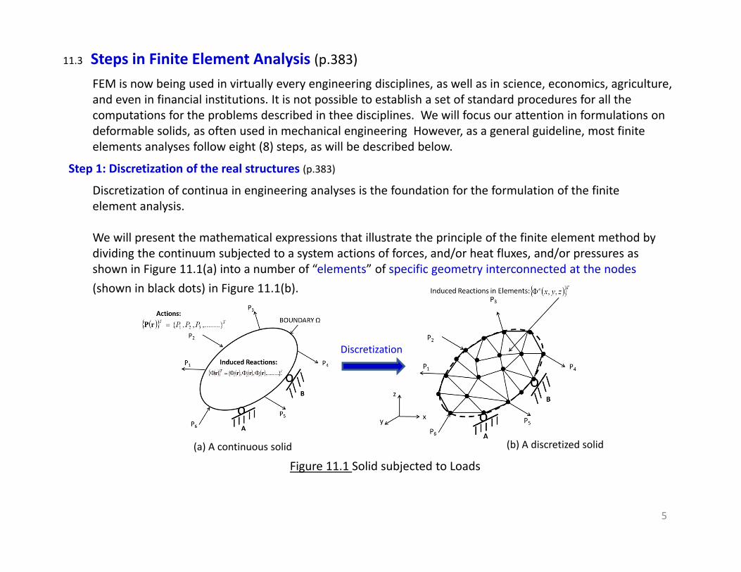
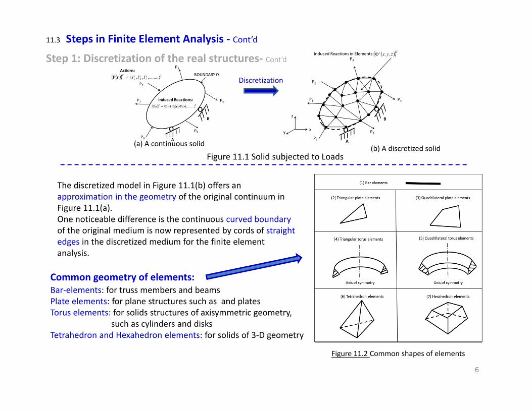
We will present the mathematical expressions that illustrate the principle of the finite element method by dividing the continuum subjected to a system actions of forces, and/or heat fluxes, and/or pressures as shown in Figure 11.1(a) into a number of “elements” of specific geometry interconnected at the nodes (shown in black dots) in Figure 11.1(b).

(a) A continuous solid (b) A discretized solid

Figure 11.1 Solid subjected to Loads

Discretization

5

6

The discretized model in Figure 11.1(b) offers an approximation in the geometry of the original continuum in Figure 11.1(a). One noticeable difference is the continuous curved boundary of the original medium is now represented by cords of straightedges in the discretized medium for the finite element analysis.

Step 1: Discretization of the real structures‐ Cont’d

11.3 Steps in Finite Element Analysis ‐ Cont’d

(a) A continuous solid (b) A discretized solidFigure 11.1 Solid subjected to Loads

Discretization

Figure 11.2 Common shapes of elements

Bar‐elements: for truss members and beamsPlate elements: for plane structures such as and platesTorus elements: for solids structures of axisymmetric geometry,

such as cylinders and disksTetrahedron and Hexahedron elements: for solids of 3‐D geometry

Common geometry of elements:

7

Step 1: Discretization of the real structures‐ Cont’d


(a) A continuous solid (b) A discretized solidFigure 11.1 Solid subjected to Loads

Discretization

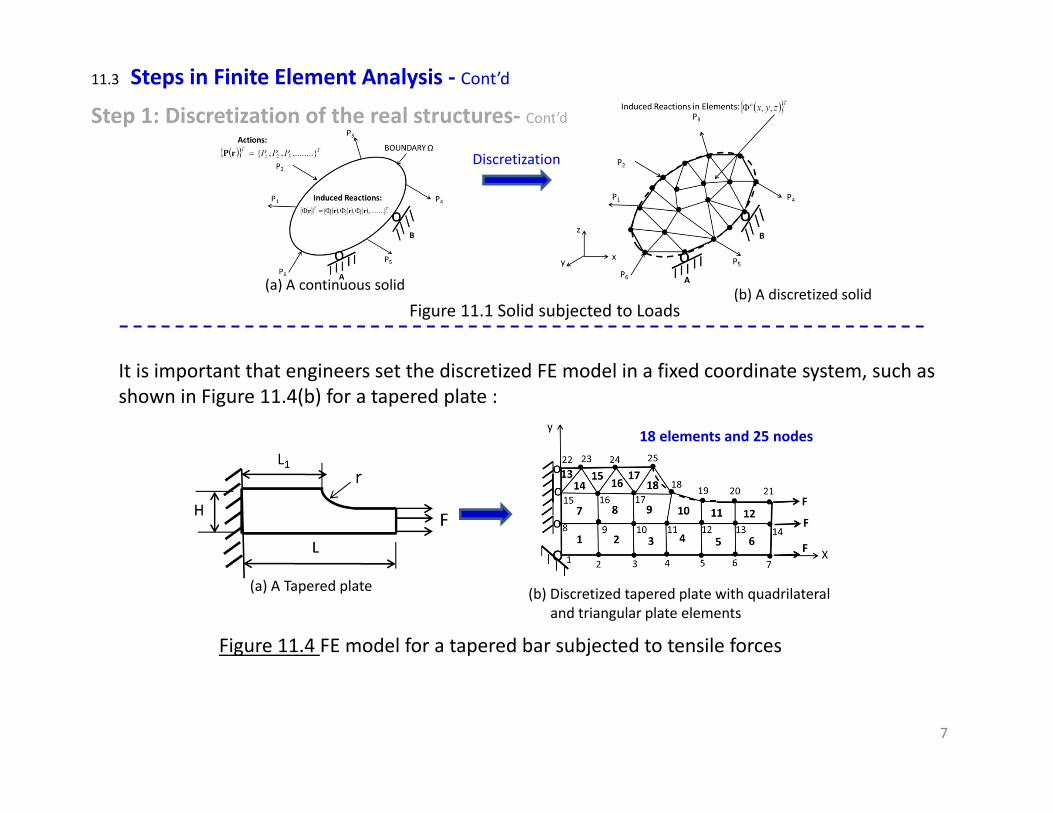
It is important that engineers set the discretized FE model in a fixed coordinate system, such as shown in Figure 11.4(b) for a tapered plate :

(a) A Tapered plate (b) Discretized tapered plate with quadrilateral and triangular plate elements

Figure 11.4 FE model for a tapered bar subjected to tensile forces

18 elements and 25 nodes

8

11.3 Steps in Finite Element Analysis ‐ Cont’dStep 1: Discretization of the real structures‐ Cont’d: Identities of elements and nodes in discretized model:

(a) A Tapered plate (b) Discretized tapered plate with quadrilateral and triangular plate elements

Node No. x‐coordinate y‐coordinate Nodal constraints

Applied nodal force

(cm) (cm) in displacements1 0 0 ux = uy = 07 18 0 F8 0 3 ux = 014 18 3 F15 0 6 ux = 017 6 618 10 619 12 421 18 4 F22 0 8 ux = 023 1.5 825 9 8

Element No.

Associate node numbers Material characterized by

input material number1 1,2,9,8 16 6,7,14,13 17 6,9,16,15 18 9,10,17,16 112 13,14,21,20 113 15,23,22,22 114 15,16,23,23 115 16,24,23,23 116 16,17,24,24 117 17,25,24,24 118 17,18,25,25 1

Nodal description of FE model of a tapered bar Element description of FE model of a tapered bar

Input of nodal and element information (18 elements and 25 nodes):

Designation of plate deformationby nodal displacements (movements):ux = displacements along x‐coordinateuy = displacements along y‐coordinate

9

Step 2: Identify the primary unknown quantities for the analysis (p.387)


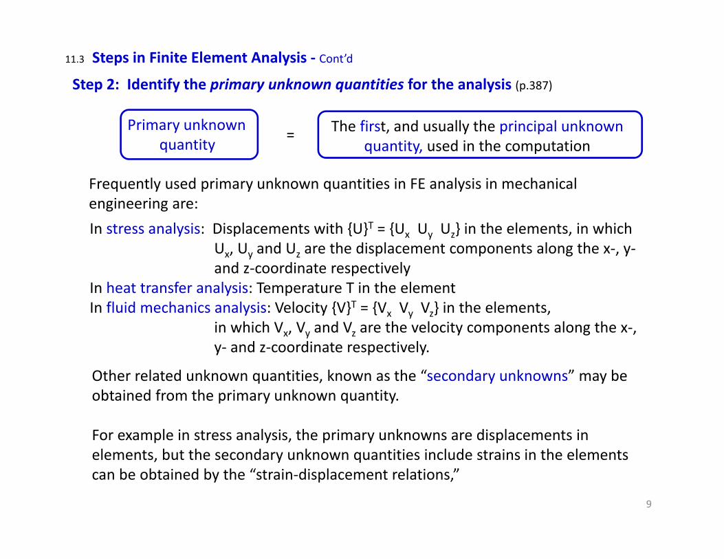
Primary unknown quantity = The first, and usually the principal unknown

quantity, used in the computation

Frequently used primary unknown quantities in FE analysis in mechanical engineering are: In stress analysis: Displacements with {U}T = {Ux Uy Uz} in the elements, in which

Ux, Uy and Uz are the displacement components along the x‐, y‐and z‐coordinate respectively

In heat transfer analysis: Temperature T in the elementIn fluid mechanics analysis: Velocity {V}T = {Vx Vy Vz} in the elements,

in which Vx, Vy and Vz are the velocity components along the x‐, y‐ and z‐coordinate respectively.

Other related unknown quantities, known as the “secondary unknowns” may be obtained from the primary unknown quantity.

For example in stress analysis, the primary unknowns are displacements in elements, but the secondary unknown quantities include strains in the elements can be obtained by the “strain‐displacement relations,”

10

Step 3: Derive the interpolation functions (p.388)11.3 Steps in Finite Element Analysis ‐ Cont’d

Interpolation functions relate the primary quantities in the elements and those at the associate nodes of the same element – a very important function in FE analysis.

General form of Interpolation function:

rr N (11.1)

rwherer = the position vector representing the respective function Φ(x,y,z) in rectangular

coordinate system, or Φ (r,θ,z) in cylindrical polar coordinate system.

= the primary unknown quantities in the element

.

The quantity [N(r)] in the right‐hand‐ side of Equation (11.1) is the interpolation function in a matrix form, and = the same primary quantities at the associate nodes of the same element.

Interpolation functions [N(r)] in Equation (11.1) often are referred to as “shape functions” because its form vary according to the “shape” of the elements.

Tetrahedral elements for 3‐D solids with 4 nodesTriangular plate elements for 2‐D plane solids have 3 nodesBar elements for 1‐D solids with 2 nodesAxisymmetric triangular elements for solids with circular geometry with 3 nodesOther element shapes: hexahedral elements have 6 sides and 8 nodes, quadrilateral plate elements with 4 sides and 4 nodes.

11

Step 3: Derive the interpolation functions‐Cont’d11.3 Steps in Finite Element Analysis ‐ Cont’d

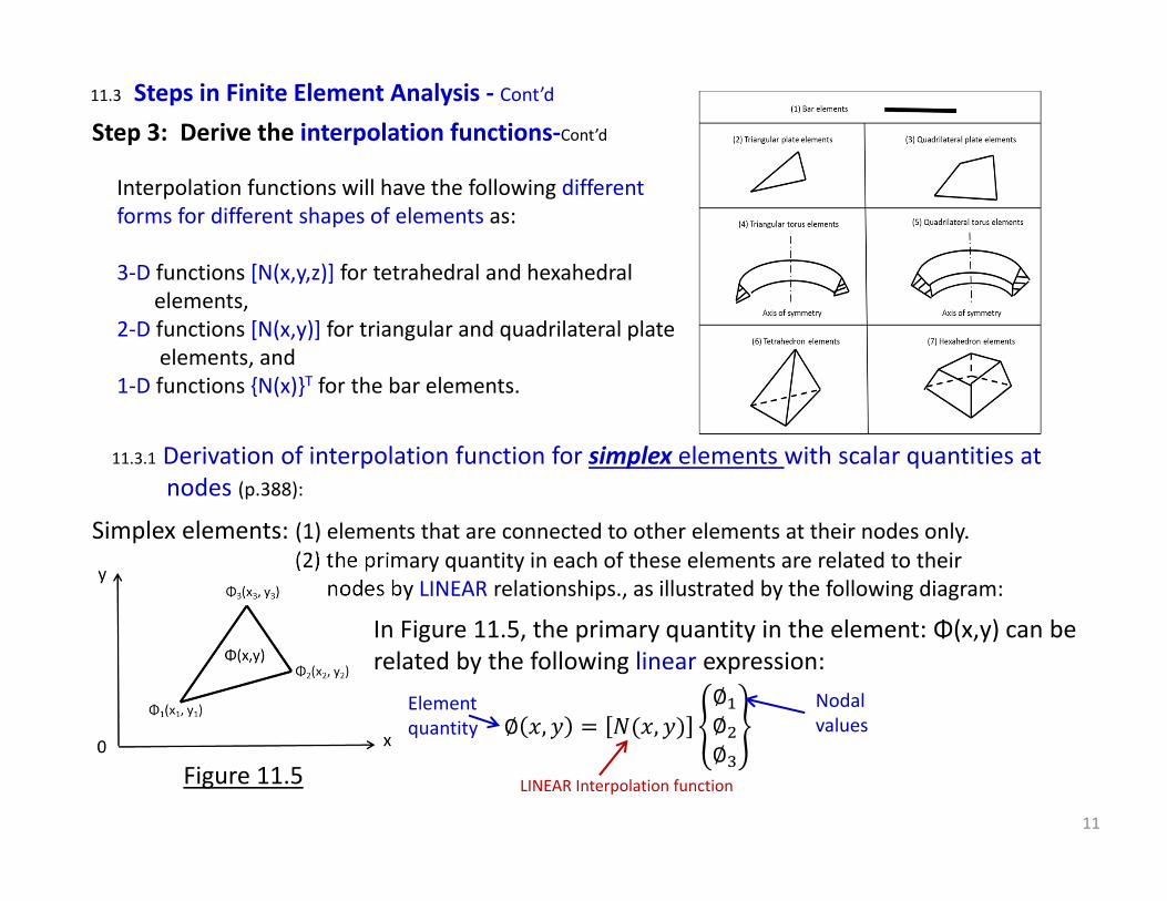
Interpolation functions will have the following different forms for different shapes of elements as:

3‐D functions [N(x,y,z)] for tetrahedral and hexahedral elements,

2‐D functions [N(x,y)] for triangular and quadrilateral plate elements, and

1‐D functions {N(x)}T for the bar elements.

11.3.1 Derivation of interpolation function for simplex elements with scalar quantities at nodes (p.388):

Simplex elements: (1) elements that are connected to other elements at their nodes only.(2) the primary quantity in each of these elements are related to their

nodes by LINEAR relationships., as illustrated by the following diagram:

In Figure 11.5, the primary quantity in the element: Φ(x,y) can be related by the following linear expression:

∅ , ,∅∅∅

Elementquantity

Nodalvalues

LINEAR Interpolation functionFigure 11.5

12


11.3.1 Derivation of interpolation function for simplex elements with Scalar quantities‐Cont’d

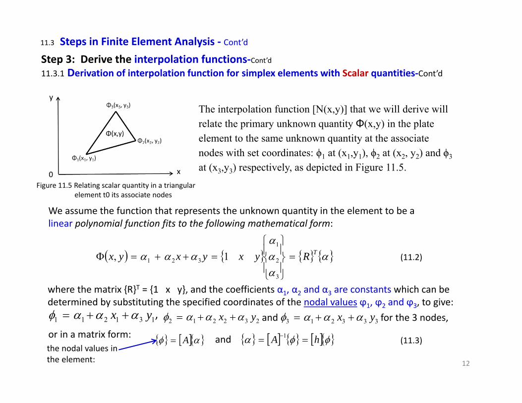
Figure 11.5 Relating scalar quantity in a triangular element t0 its associate nodes

The interpolation function [N(x,y)] that we will derive will relate the primary unknown quantity Φ(x,y) in the plate element to the same unknown quantity at the associate nodes with set coordinates: ϕ1 at (x1,y1), ϕ2 at (x2, y2) and ϕ3

at (x3,y3) respectively, as depicted in Figure 11.5.

We assume the function that represents the unknown quantity in the element to be a linear polynomial function fits to the following mathematical form:

TRyxyxyx

3

2

1

321 1, (11.2)

where the matrix {R}T = {1 x y}, and the coefficients α1, α2 and α3 are constants which can be determined by substituting the specified coordinates of the nodal values ϕ1, ϕ2 and ϕ3, to give:

131211 yx 232212 yx 333213 yx

or in a matrix form: A (11.3) hA 1and

for the 3 nodes,

the nodal values in the element:

, and

13


11.3.1 Derivation of interpolation function for simplex elements with Scalar quantities – Cont’d

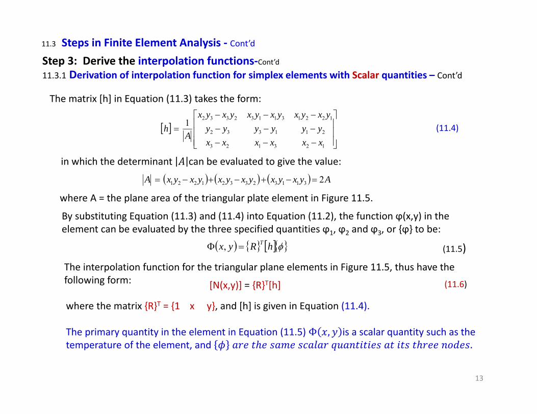
The matrix [h] in Equation (11.3) takes the form:

123123

211332

1221311323321

xxxxxxyyyyyy

yxyxyxyxyxyx

Ah (11.4)

in which the determinant can be evaluated to give the value:

AyxyxyxyxyxyxA 2311323321221

where A = the plane area of the triangular plate element in Figure 11.5.

By substituting Equation (11.3) and (11.4) into Equation (11.2), the function ϕ(x,y) in the element can be evaluated by the three specified quantities ϕ1, ϕ2 and ϕ3, or {ϕ} to be:

hRyx T , (11.5)The interpolation function for the triangular plane elements in Figure 11.5, thus have the following form: [N(x,y)] = {R}T[h] (11.6)

where the matrix {R}T = {1 x y}, and [h] is given in Equation (11.4).

The primary quantity in the element in Equation (11.5) Φ , is a scalar quantity such as the temperature of the element, and .

14


11.3.1 Derivation of interpolation function for simplex elements with scalar quantities at nodes – Cont’d:

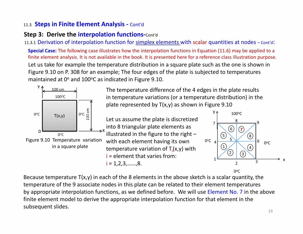
Let us take for example the temperature distribution in a square plate such as the one is shown in Figure 9.10 on P. 308 for an example; The four edges of the plate is subjected to temperatures maintained at 0o and 100oC as indicated in Figure 9.10.

Figure 9.10 Temperature variationin a square plate

The temperature difference of the 4 edges in the plate resultsin temperature variations (or a temperature distribution) in theplate represented by T(x,y) as shown in Figure 9.10

Let us assume the plate is discretized into 8 triangular plate elements as illustrated in the figure to the right –with each element having its own temperature variation of Ti(x,y) with i = element that varies from: i = 1,2,3,……,8.

Because temperature T(x,y) in each of the 8 elements in the above sketch is a scalar quantity, the temperature of the 9 associate nodes in this plate can be related to their element temperatures by appropriate interpolation functions, as we defined before. We will use Element No. 7 in the above finite element model to derive the appropriate interpolation function for that element in the subsequent slides.

Special Case: The following case illustrates how the interpolation functions in Equation (11.6) may be applied to a finite element analysis. It is not available in the book. It is presented here for a reference class illustration purpose.



Figure A

Figure B

Figure C

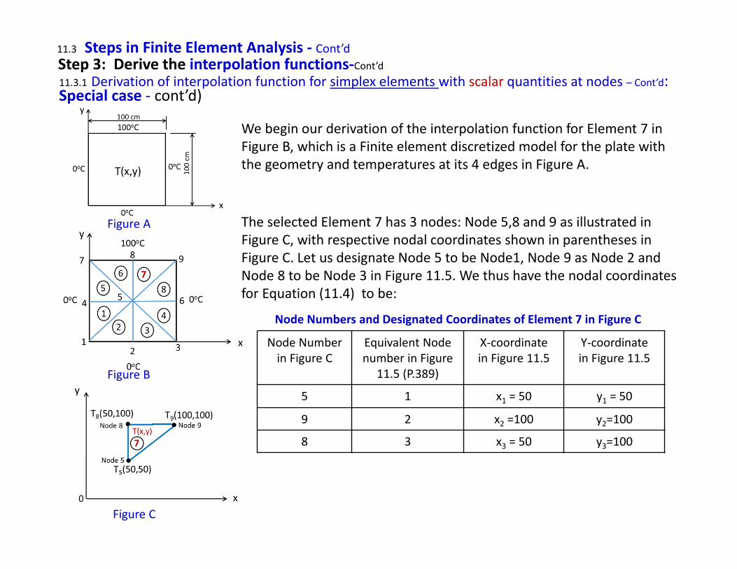
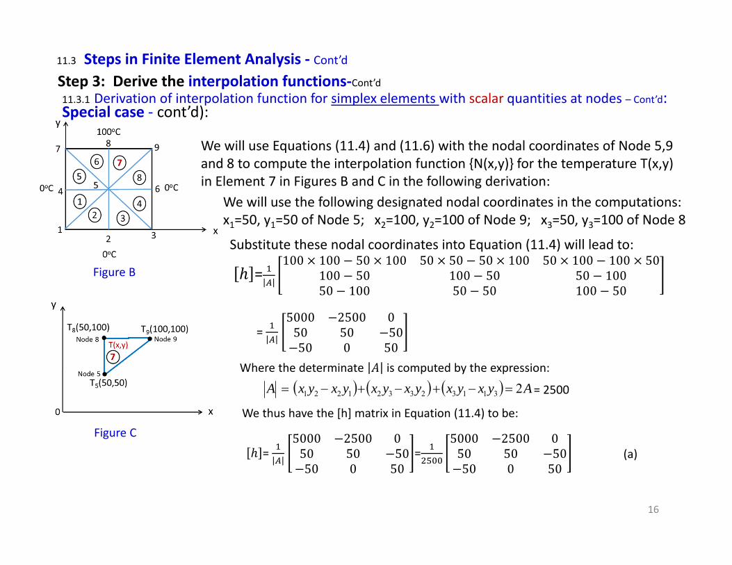
We begin our derivation of the interpolation function for Element 7 in Figure B, which is a Finite element discretized model for the plate withthe geometry and temperatures at its 4 edges in Figure A.

The selected Element 7 has 3 nodes: Node 5,8 and 9 as illustrated in Figure C, with respective nodal coordinates shown in parentheses in Figure C. Let us designate Node 5 to be Node1, Node 9 as Node 2 and Node 8 to be Node 3 in Figure 11.5. We thus have the nodal coordinates for Equation (11.4) to be:

Node Numberin Figure C

Equivalent Node number in Figure

11.5 (P.389)

X‐coordinatein Figure 11.5

Y‐coordinatein Figure 11.5

5 1 x1 = 50 y1 = 50

9 2 x2 =100 y2=100

8 3 x3 = 50 y3=100

Node Numbers and Designated Coordinates of Element 7 in Figure C

Special case ‐ cont’d)

16



Figure B

Figure C

We will use Equations (11.4) and (11.6) with the nodal coordinates of Node 5,9 and 8 to compute the interpolation function {N(x,y)} for the temperature T(x,y) in Element 7 in Figures B and C in the following derivation:

We will use the following designated nodal coordinates in the computations:x1=50, y1=50 of Node 5; x2=100, y2=100 of Node 9; x3=50, y3=100 of Node 8

Substitute these nodal coordinates into Equation (11.4) will lead to:

=100 100 50 100 50 50 50 100 50 100 100 50

100 50 100 50 50 10050 100 50 50 100 50

= 5000 2500 050 50 5050 0 50

Where the determinate is computed by the expression:

AyxyxyxyxyxyxA 2311323321221 = 2500

We thus have the [h] matrix in Equation (11.4) to be:

= 5000 2500 050 50 5050 0 50

=5000 2500 050 50 5050 0 50

(a)

Special case ‐ cont’d):

17



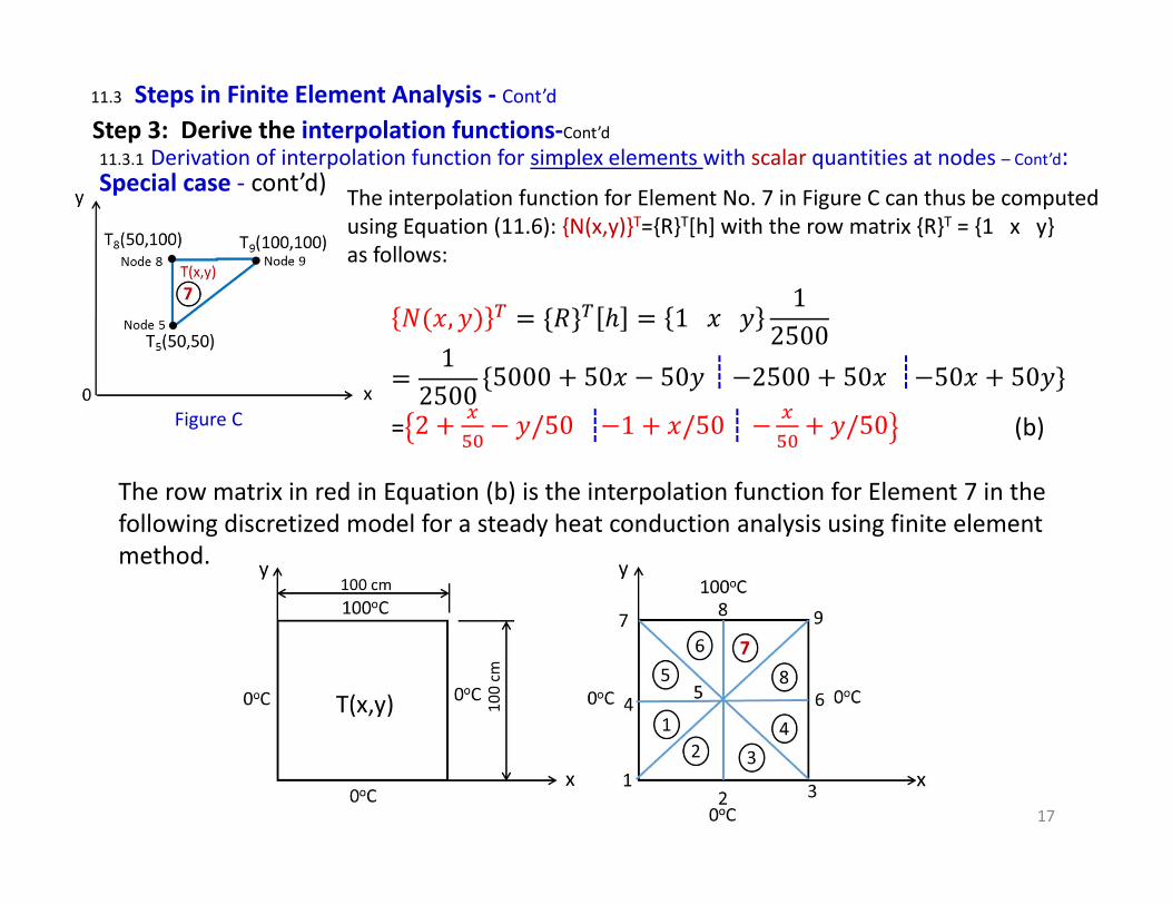
Figure C

The interpolation function for Element No. 7 in Figure C can thus be computedusing Equation (11.6): {N(x,y)}T={R}T[h] with the row matrix {R}T = {1 x y} as follows:

, 1 1

25001

25005000 50 50 2500 50 50 50

= 2 /50 1 /50 /50 (b)

The row matrix in red in Equation (b) is the interpolation function for Element 7 in thefollowing discretized model for a steady heat conduction analysis using finite elementmethod.

Special case ‐ cont’d)

18



Example on using the interpolation function in FE analyses:We define interpolation function [N(x,y)] to be the function that relate the NODAL qyanties to thatanywhere in the corresponding elements, as expressed below:

∅ , ,∅∅∅

Elementquantity

Nodalvalues

Interpolation function

Here, we will compute the interpolation function of a triangular element with designated nodalcoordinates as illustrated as given in Equation (b) in the last slide, which allows us to express thetemperature anywhere in this element (Element 7 in the FE model), such as Tp(60,70) with the element at x=60 cm and y=70 cm, in terms of its nodal temperatures T5 =25.2oC, T9 =50oC and T8 =100oC result

from a finite element analysis:

Tp(60,75) = {(2+60/50‐70/50) (‐1+60/50) (60/50+70/50)}

= 1.8 0.2 0.225.250100

67.36

The interpolation function of an element would enable us compute the scalar quantities (such as temperature) anywhere in the element based on computed nodal temperatures.

Special case ‐ end

19


11.3.2 Derivation of interpolation function for simplex elements with Vector quantities at nodes (p.390)

Often, the primary unknown quantities in triangular plate elements in a discretized finite element model contain VECTOR quantities with more than two components.

Components in its primary quantity expressed as Φx(x,y) along the x‐coordinate and the other component Φy(x,y) along the y‐coordinate asillustrated in Figure 11.6.

Consequently, there are 2 or 3 corresponding components of the same primary quantity: at each of the 3 associate nodes: (1) φ1x(x1,y1) along the x‐direction, and(2) φ1y(x1,y1) along the y‐coordinate at Node 1

situated at (x1,y1), etc.

Figure 11.6 Triangular Plate Element with Two Unknown Components

A common practice of FE analysis involving primary unknown vectors is in the stress analysis of machine structures with element displacements U(x,y) to be the primary unknown quantity with 2 components along the x‐ and y‐coordinates respectively. Interpolation functions for this situation require more complicated mathematical derivations than those for scalar quantities as presented in the previous sub‐section.

20


11.3.2 Derivation of interpolation function for simplex elements with Vector quantities at nodes

By referring the triangular plate element in Figure 11.6,we may express the element vectorial quantities in terms of the same quantities at its 3 nodes by the following expression:

333

222

111

321

654

321

,,,

,,,,

,,

,

yxyxyx

yxNyxNyxNyxN

yxyx

yxyx

yxy

x

(11.8)

Element Quantities:

Interpolation Function

NodalQuantities:

Equation (11.7) shows that the vector quantities in the element vary LINEARLY over the element, as in all simplex elements. N1(x,y), N2(x,y) and N3(x,y) in Equation (11.8) are components of the interpolation function [N(x,y)] associated with the unknown nodal quantities ϕ1, ϕ2, and ϕ3 at Node 1, 2 and 3 respectively:

111

1111 ,

,yxyx

y

x

222

2222 ,

,yxyx

y

x

333

3333 ,

,yxyx

y

x

(11.7)

yxxxyyyxyxA

yxN 2332233211,

yxxxyyyxyxA

yxN 3113311321,

yxxxyyyxyxA

yxN 1221122131,

(11.9a)

(11.9b)

(11.9c) 3113233212212

1 yxyxyxyxyxyxA where = plane area of the element

The components of the interpolation function are expressed to be:

Figure 11.6

21



333

222

111

321

654

321

,,,

,,,,

,,

,

yxyxyx

yxNyxNyxNyxN

yxyx

yxyx

yxy

x

(11.8)

111

1111 ,

,yxyx

y

x

222

2222 ,

,yxyx

y

x

333

3333 ,

,yxyx

y

x

where, and

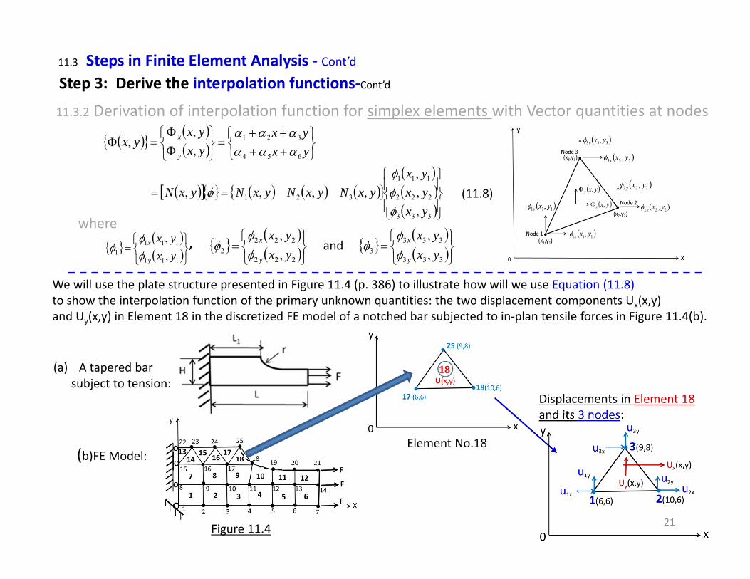
We will use the plate structure presented in Figure 11.4 (p. 386) to illustrate how will we use Equation (11.8)to show the interpolation function of the primary unknown quantities: the two displacement components Ux(x,y) and Uy(x,y) in Element 18 in the discretized FE model of a notched bar subjected to in‐plan tensile forces in Figure 11.4(b).

Figure 11.4

(a) A tapered barsubject to tension:

(b)FE Model:Element No.18

Displacements in Element 18and its 3 nodes:

22

By referring to displacements Ux(x,y) and Uy(x,y) in Element 18 and those of the 3 nodes: (u1x, u1y) at Node 1, (u2x, u2y) at Node 2, and (u3x, u3y) at Node 3 in the up right figure with nodal coordinates: x1=6, x2=10, x3=9; y1=6, y2=6, y3=8, as shown in Figure 11.4(b) using Equations (11.9a,b,c):



We will first compute the plane area of Element 18 to be:12

= 6 6 10 6 10 8 9 6 9 6 6 8 = 8 4 18

We will then use Equations (11.9a,b,c) to compute the 3 components , N1(x,y), N2(x,y) and N3(x,y)of the interpolation function as:

,14 10 8 9 6 6 8 9 10 6.5 0.5 0.25

(x,y)= 9 6 6 8 8 6 + 6 9 1.5 0.5 0.75

(x,y) = 6 6 10 6 6 6 10 6 6

23


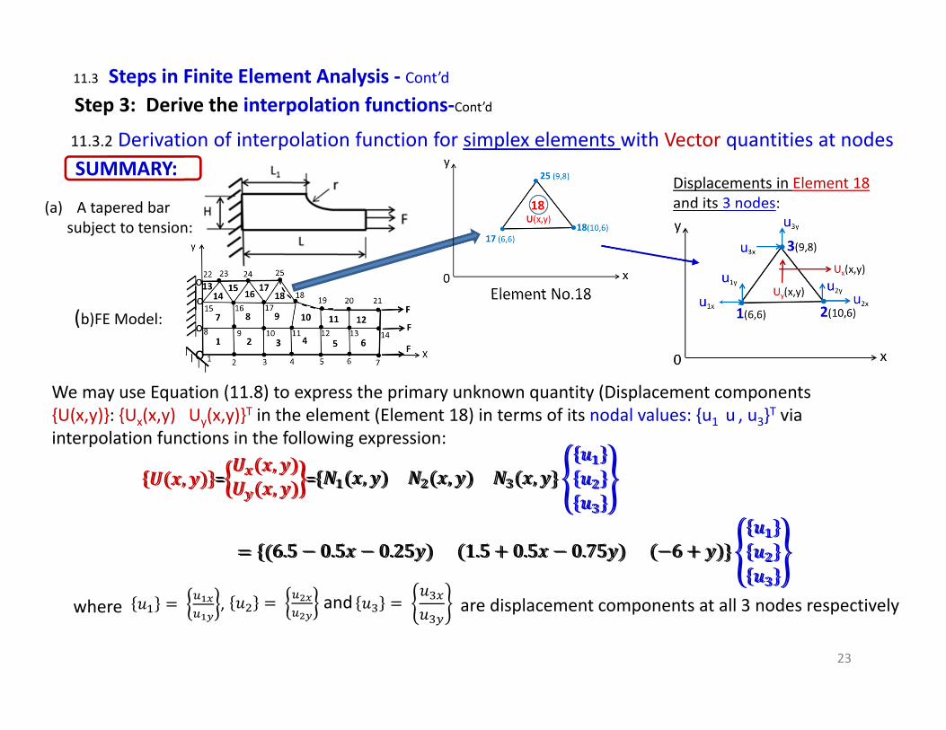
11.3.2 Derivation of interpolation function for simplex elements with Vector quantities at nodes SUMMARY:Y

(a) A tapered barsubject to tension:

(b)FE Model:Element No.18

Displacements in Element 18and its 3 nodes:

We may use Equation (11.8) to express the primary unknown quantity (Displacement components{U(x,y)}: {Ux(x,y) Uy(x,y)}T in the element (Element 18) in terms of its nodal values: {u1 u , u3}T via interpolation functions in the following expression:

, =,, = , , ,

6.5 0.5 0.25 1.5 0.5 0.75 6

,

, =,, = , , ,

6.5 0.5 0.25 1.5 0.5 0.75 6

and where are displacement components at all 3 nodes respectively

24

Step 3: Derive the interpolation functions‐Cont’d



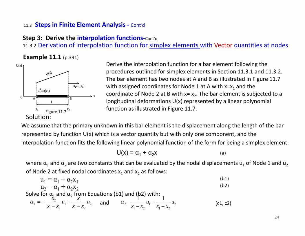
Example 11.1 (p.391)Derive the interpolation function for a bar element following the procedures outlined for simplex elements in Section 11.3.1 and 11.3.2. The bar element has two nodes at A and B as illustrated in Figure 11.7 with assigned coordinates for Node 1 at A with x=x1 and the coordinate of Node 2 at B with x= x2. The bar element is subjected to a longitudinal deformations U(x) represented by a linear polynomial function as illustrated in Figure 11.7. Figure 11.7

Solution:We assume that the primary unknown in this bar element is the displacement along the length of the bar represented by function U(x) which is a vector quantity but with only one component, and the interpolation function fits the following linear polynomial function of the form for being a simplex element:

U(x) = α1 + α2x (a)

where α1 and α2 are two constants that can be evaluated by the nodal displacements u1 of Node 1 and u2of Node 2 at fixed nodal coordinates x1 and x2 as follows:

u1 = α1 + α2x1u2 = α1 + α2x2

(b1)(b2)

Solve for α1 and α2 from Equations (b1) and (b2) with:2

21

11

21

21 u

xxxu

xxx

2

211

212

11 uxx

uxx

and (c1, c2)

25

Step 3: Derive the interpolation functions‐Cont’d



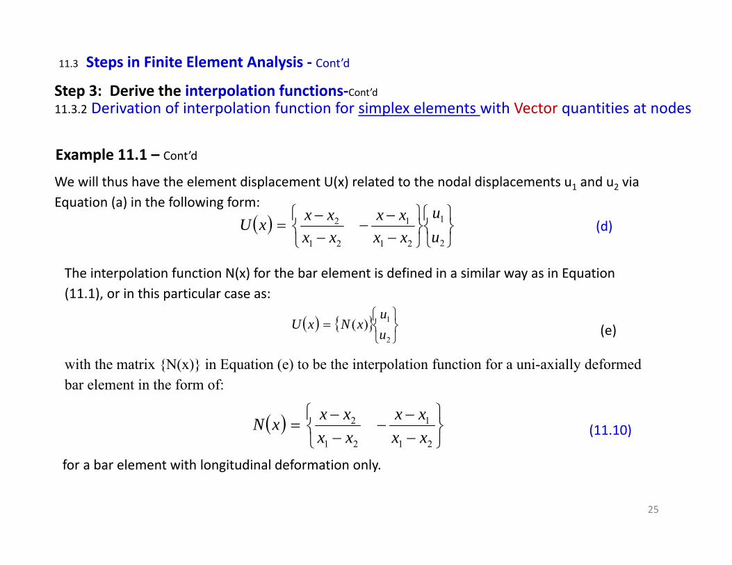
Example 11.1 – Cont’d

We will thus have the element displacement U(x) related to the nodal displacements u1 and u2 via Equation (a) in the following form:

2

1

21

1

21

2

uu

xxxx

xxxxxU (d)

The interpolation function N(x) for the bar element is defined in a similar way as in Equation (11.1), or in this particular case as:

2

1)(uu

xNxU

with the matrix {N(x)} in Equation (e) to be the interpolation function for a uni-axially deformed bar element in the form of:

(e)

21

1

21

2

xxxx

xxxxxN (11.10)

for a bar element with longitudinal deformation only.

26

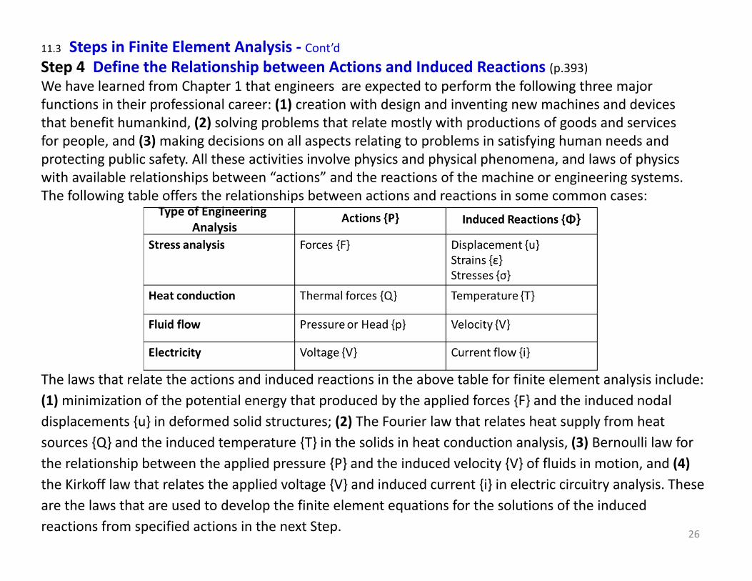
11.3 Steps in Finite Element Analysis ‐ Cont’dStep 4 Define the Relationship between Actions and Induced Reactions (p.393)We have learned from Chapter 1 that engineers are expected to perform the following three major functions in their professional career: (1) creation with design and inventing new machines and devices that benefit humankind, (2) solving problems that relate mostly with productions of goods and servicesfor people, and (3)making decisions on all aspects relating to problems in satisfying human needs and protecting public safety. All these activities involve physics and physical phenomena, and laws of physics with available relationships between “actions” and the reactions of the machine or engineering systems. The following table offers the relationships between actions and reactions in some common cases:

Type of Engineering Analysis

The laws that relate the actions and induced reactions in the above table for finite element analysis include: (1)minimization of the potential energy that produced by the applied forces {F} and the induced nodal displacements {u} in deformed solid structures; (2) The Fourier law that relates heat supply from heat sources {Q} and the induced temperature {T} in the solids in heat conduction analysis, (3) Bernoulli law for the relationship between the applied pressure {P} and the induced velocity {V} of fluids in motion, and (4)the Kirkoff law that relates the applied voltage {V} and induced current {i} in electric circuitry analysis. These are the laws that are used to develop the finite element equations for the solutions of the induced reactions from specified actions in the next Step.

27

11.3 Steps in Finite Element Analysis ‐ Cont’dStep 5 Derive Element Equations (p.394)Element equations relate the applied actions to the discretized continua and the induced reactions in the elements. There are generally two distinct methods that can be used to derive these equations in finite element analyses:

(1) The Rayleigh-Ritz method:We began this chapter with the presentation of the principle of the Finite element method (FEM) with the discretization of continua in Figure 11.1(a) on p.384 into a finite number of individual elements of specific geometry interconnected at a finite number of nodes in Figure 11.1(b).

Figure 11.1(a) Figure 11.1(b)

Derivation of element equations for the elements in Figure 11.1(b) is based on the identification of the expressionof a FUNCTIONAL (function of functions) that include the primary unknown quantities, e.g. the induced displacement in the elements and the applied actions, namely the applied forces or pressures. This functional can be used to relate the actions and the induced reactions of the discretized continua according to law of physics for all elements in the discretized FE model, as illustrated in Figure 11.1(b). We will derive the appropriate math expression for the FUNCTIONALS in the next slide.

28

11.3 Steps in Finite Element Analysis ‐ Cont’dStep 5 Derive Element Equations – Cont’d(1) The Rayleigh-Ritz method - Cont’d:

eThis method involves with variation of a suitable functional that can characterize the continuum in the analysis with Φe being the primary unknown quantity in the elements of a discretized continuum in Figure 11.1(b). This functional can be expressed in forms of differential quantities such as shown in Equation (11.11).

dsr

gdvr

fs

ee

v

eee

,.........,,........, (11.11)

where dv and ds are the volume and surface of the elements in the discretized continuum respectively as shown in Figure 11.1(b).

Figure 11.1(b)

The variational principle leads to the situation in which the rate of change of the functional in Equation (11.11) with respect to its variable Φe to be kept in minimum as shown in Equation (11.12)

0

.

.

.3

2

1

e

e

e

e

e

(11.12)

where ................,,, 321eee are the primary quantities in respective elements 1,2,3,….in the discretized

medium as shown in Figure 11.1(b).

e

29

11.3 Steps in Finite Element Analysis ‐ Cont’dStep 5 Derive Element Equations – Cont’d(1) The Rayleigh-Ritz method - Cont’d:

0

.

.

.3

2

1

e

e

e

e

e

(11.12)

Figure 11.1(b)

The variation of the functional with respect to the induced quantities in a continua to a minimum as shownin Equation (11.12) is quite commonly used practice in describing a continuum in equilibrium condition, such asthe potential energy produced by the displacements in the continuum induced by applied forces, or the induced temperature field in a substance induced by applied thermal forces. The expression in Equation (11.12) also applies to EACH element in a discretized continuum as illustrated in Figure 11.1(b), as will be demonstrated by the following equations:

01

e

02

e

03

e

for Element No. 1

for Element No. 2

for Element No. 3

(11.13a)

(11.13b)

(11.13c)

and so on and so forth. Equation (11.13a,b,c) may lead to the “element equation” for all elements of a discretized continuum in Figure 11.1(b)

30

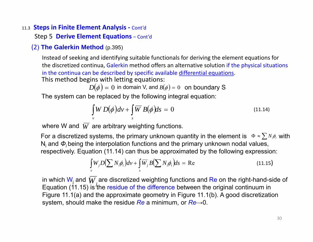
11.3 Steps in Finite Element Analysis ‐ Cont’dStep 5 Derive Element Equations – Cont’d(2) The Galerkin Method (p.395)

Instead of seeking and identifying suitable functionals for deriving the element equations for the discretized continua, Galerkin method offers an alternative solution if the physical situationsin the continua can be described by specific available differential equations.

0D in domain V, and 0B on boundary SThe system can be replaced by the following integral equation:

0 dsBWdvDWsv

(11.14)

where W and W are arbitrary weighting functions.For a discretized systems, the primary unknown quantity in the element is withNi and Φi being the interpolation functions and the primary unknown nodal values, respectively. Equation (11.14) can thus be approximated by the following expression:

iiN

Re dsNBWdvNDW iis

jiiv

j (11.15)

in which Wj and are discretized weighting functions and Re on the right-hand-side of Equation (11.15) is the residue of the difference between the original continuum in Figure 11.1(a) and the approximate geometry in Figure 11.1(b). A good discretization system, should make the residue Re a minimum, or Re→0.

jW

This method begins with letting equations:

31

11.3 Steps in Finite Element Analysis ‐ Cont’dStep 5 Derive Element Equations – Cont’d(2) The Galerkin Method – Cont’d

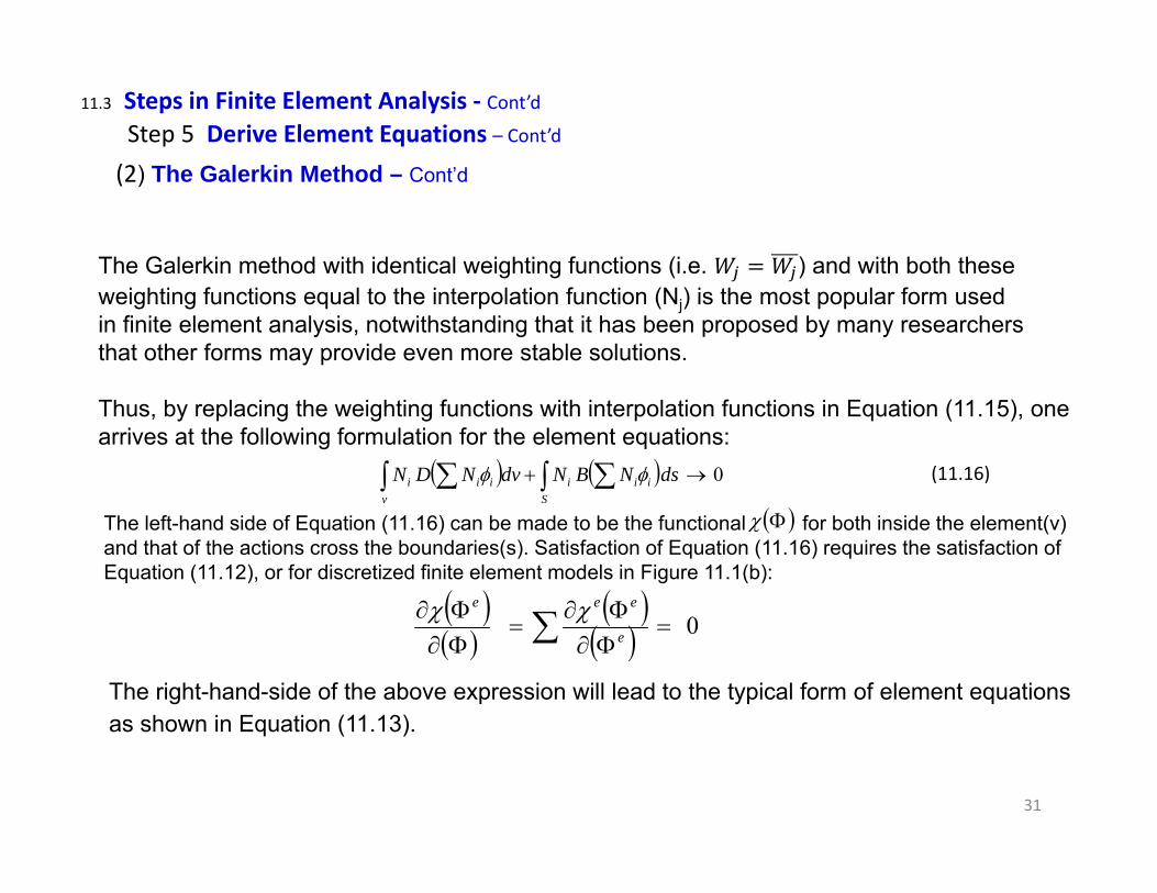
The Galerkin method with identical weighting functions (i.e. ) and with both these weighting functions equal to the interpolation function (Nj) is the most popular form used in finite element analysis, notwithstanding that it has been proposed by many researchers that other forms may provide even more stable solutions.

Thus, by replacing the weighting functions with interpolation functions in Equation (11.15), one arrives at the following formulation for the element equations:

0 dsNBNdvNDN iiS

iiiv

i (11.16)

The left-hand side of Equation (11.16) can be made to be the functional for both inside the element(v) and that of the actions cross the boundaries(s). Satisfaction of Equation (11.16) requires the satisfaction of Equation (11.12), or for discretized finite element models in Figure 11.1(b):

0

e

eee

The right-hand-side of the above expression will lead to the typical form of element equations as shown in Equation (11.13).

11.3 Steps in Finite Element Analysis ‐ Cont’dStep 5 Derive Element Equations – Cont’d

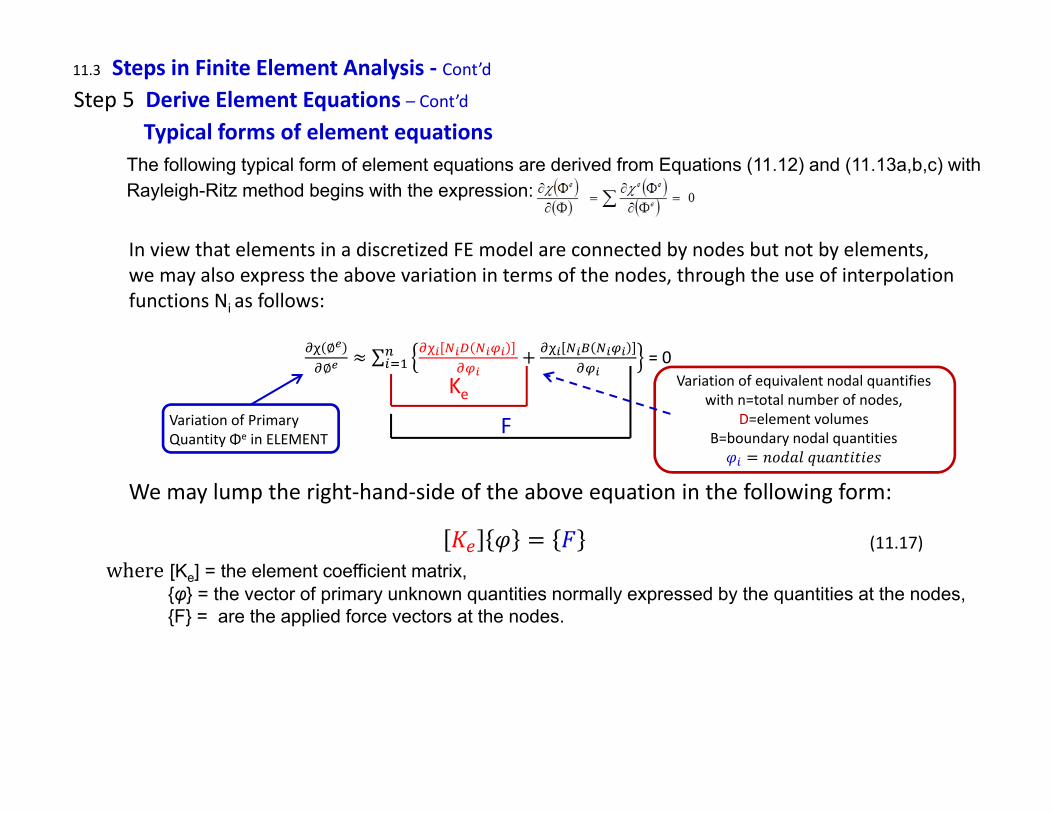
Typical forms of element equationsThe following typical form of element equations are derived from Equations (11.12) and (11.13a,b,c) with Rayleigh-Ritz method begins with the expression:

(11.17)where [Ke] = the element coefficient matrix,

{φ} = the vector of primary unknown quantities normally expressed by the quantities at the nodes,{F} = are the applied force vectors at the nodes.

In view that elements in a discretized FE model are connected by nodes but not by elements,we may also express the above variation in terms of the nodes, through the use of interpolation functions Ni as follows:

∅∅

∑ = 0

Variation of PrimaryQuantity Φe in ELEMENT

Variation of equivalent nodal quantifieswith n=total number of nodes,

D=element volumesB=boundary nodal quantities

KeF

We may lump the right‐hand‐side of the above equation in the following form:

33

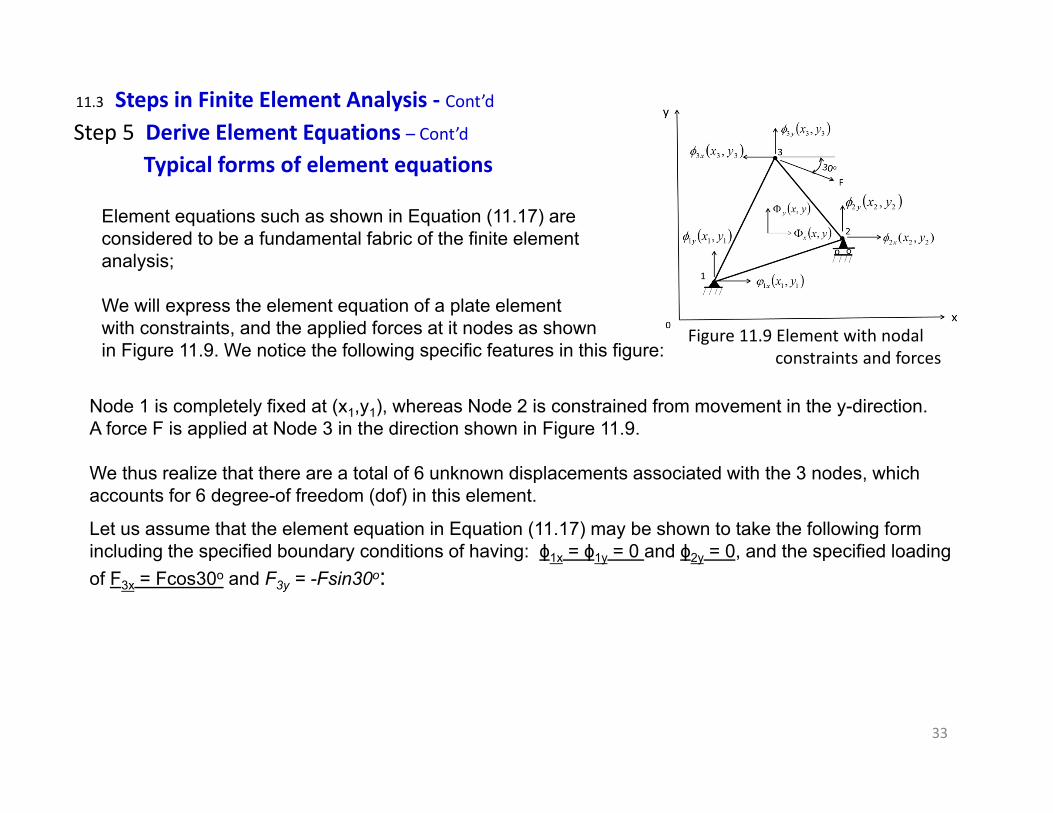
Node 1 is completely fixed at (x1,y1), whereas Node 2 is constrained from movement in the y-direction. A force F is applied at Node 3 in the direction shown in Figure 11.9.

We thus realize that there are a total of 6 unknown displacements associated with the 3 nodes, which accounts for 6 degree-of freedom (dof) in this element.

Element equations such as shown in Equation (11.17) are considered to be a fundamental fabric of the finite element analysis;

We will express the element equation of a plate element with constraints, and the applied forces at it nodes as shown in Figure 11.9. We notice the following specific features in this figure:

Step 5 Derive Element Equations – Cont’dTypical forms of element equations


Figure 11.9 Element with nodal constraints and forces

Let us assume that the element equation in Equation (11.17) may be shown to take the following form including the specified boundary conditions of having: ϕ1x = ϕ1y = 0 and ϕ2y = 0, and the specified loading of F3x = Fcos30o and F3y = -Fsin30o:

34

11.3 Steps in Finite Element Analysis ‐ Cont’dStep 5 Derive Element Equations – Cont’dTypical forms of element equations (p.397)‐ cont’d

oy

ox

y

x

y

x

y

x

y

x

y

x

FFFF

FFFF

kkkkkkkkkkkkkkkkkkkkkkkkkkkkkkkkkkkk

30sin30cos

0000

0

00

3

3

2

2

1

1

3

3

2

2

1

1

666564636261

565554535251

464544434241

363534333231

262524232221

161514131211

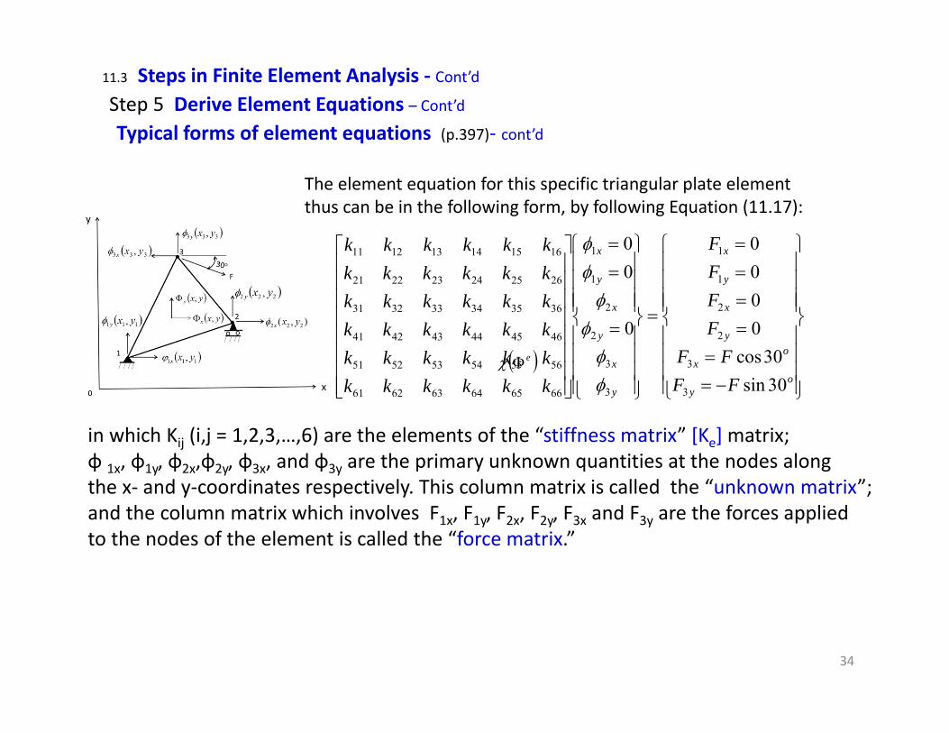
The element equation for this specific triangular plate elementthus can be in the following form, by following Equation (11.17):

in which Kij (i,j = 1,2,3,…,6) are the elements of the “stiffness matrix” [Ke] matrix;φ 1x, φ1y, φ2x,φ2y, φ3x, and φ3y are the primary unknown quantities at the nodes along the x‐ and y‐coordinates respectively. This column matrix is called the “unknown matrix”; and the column matrix which involves F1x, F1y, F2x, F2y, F3x and F3y are the forces applied to the nodes of the element is called the “force matrix.”

e

35

Step 6 Derive Overall Stiffness Equations11.3 Steps in Finite Element Analysis ‐ Cont’d

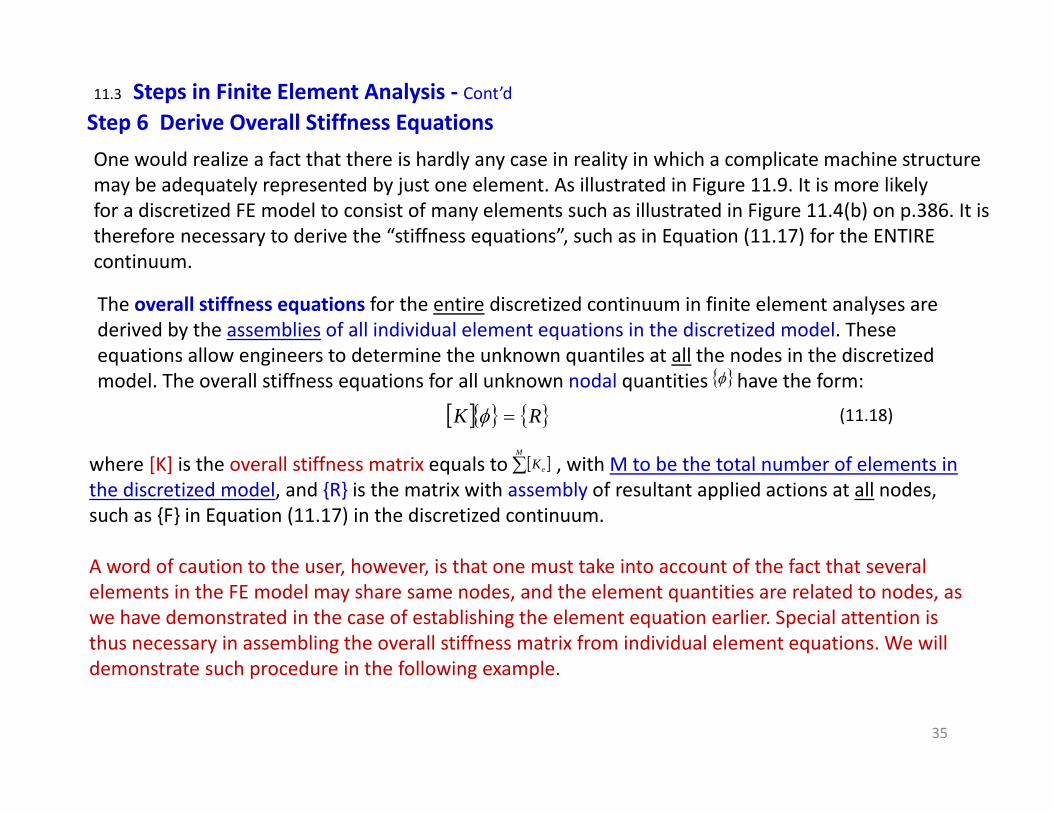
One would realize a fact that there is hardly any case in reality in which a complicate machine structuremay be adequately represented by just one element. As illustrated in Figure 11.9. It is more likelyfor a discretized FE model to consist of many elements such as illustrated in Figure 11.4(b) on p.386. It is therefore necessary to derive the “stiffness equations”, such as in Equation (11.17) for the ENTIREcontinuum.

The overall stiffness equations for the entire discretized continuum in finite element analyses are derived by the assemblies of all individual element equations in the discretized model. These equations allow engineers to determine the unknown quantiles at all the nodes in the discretized model. The overall stiffness equations for all unknown nodal quantities have the form:

RK (11.18)

where [K] is the overall stiffness matrix equals to , with M to be the total number of elements in the discretized model, and {R} is the matrix with assembly of resultant applied actions at all nodes, such as {F} in Equation (11.17) in the discretized continuum.

A word of caution to the user, however, is that one must take into account of the fact that several elements in the FE model may share same nodes, and the element quantities are related to nodes, aswe have demonstrated in the case of establishing the element equation earlier. Special attention is thus necessary in assembling the overall stiffness matrix from individual element equations. We will demonstrate such procedure in the following example.

M

eK

36

Step 6 Derive Overall Stiffness Equations – Cont’d11.3 Steps in Finite Element Analysis ‐ Cont’d

Example 11.3 (P.397):A thin plate of quadrilateral shape is shown in Figure 11.10. The plate is sub‐divided into to two triangular elements with Element 1 consisting of Node 1, 3 and 4, and Element 2 has Node 2, 4 and 3. It shows that Node 3 and 4 are shared by both Element 1 and 2. We will draw a map for the assembly of these two element equations to form the overall stiffness equation for the plate structure if the element equations for both Elements 1 and 2 are expressed in Equations (a) and (b) respectively. Figure 11.10 FE model of a quadrilateral

plate structure

y

x

y

x

y

x

y

x

y

x

y

x

FFFFFF

vuvuvu

4

4

3

3

1

1

4

4

3

3

1

1

y

x

y

x

y

x

y

x

y

x

y

x

FFFFFF

vuvuvu

4

4

3

3

2

2

4

4

3

3

2

2

(a)

(b)

For Element No. 1:

For Element No. 2:

The open triangles (Δ) and solid circles (●) in Equations (a) and (b) represent the elements of coefficient matrix [Ke1] for Element 1, and [Ke2] for Element 2 respectively.

37


Example 11.3 (P.397) – Cont’d on assembly of coefficient matrices:Step 6 Derive Overall Stiffness Equations – Cont’d

We recognize the following facts from the FE discretization of theplate structure in Figure 11.10:

(1) There are 4 nodes in the FE model.(2) Each node has 2 dof: with ui (i=1,2,3,4) to be the nodal displacements

along the x‐coordinate, and vi (i=1,2,3,4) are the displacements along the y‐coordinate.

(3) So, the overall stiffness matrix [K] in Equation (11.18) should have8 rows and 8 columns to coincide with 2x4=8dof (degree‐of‐freedom).

(4) If we express the nodal displacements in the following way:(a column matrix with 8 elements):

Figure 11.10 FE model of a quadrilateral plate structure

We should then have the map for the assembly of these two element equations to form the overall stiffness equationfor the plate structure in the form as shown in Figure 11.11 inthe left.

Figure 11.11 Map of the assembled coefficient matrix [K] of Element 1 and 2

38

11.3 Steps in Finite Element Analysis ‐ Cont’dStep 7 Solve for Primary Unknown Quantities (p.398)

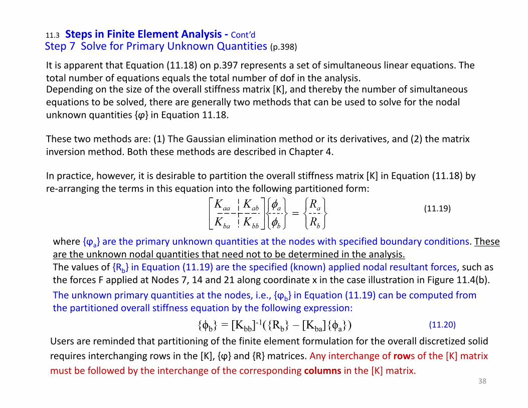
It is apparent that Equation (11.18) on p.397 represents a set of simultaneous linear equations. The total number of equations equals the total number of dof in the analysis. Depending on the size of the overall stiffness matrix [K], and thereby the number of simultaneous equations to be solved, there are generally two methods that can be used to solve for the nodal unknown quantities {φ} in Equation 11.18.

These two methods are: (1) The Gaussian elimination method or its derivatives, and (2) the matrix inversion method. Both these methods are described in Chapter 4.

In practice, however, it is desirable to partition the overall stiffness matrix [K] in Equation (11.18) by re‐arranging the terms in this equation into the following partitioned form:

(11.19)

where {ϕa} are the primary unknown quantities at the nodes with specified boundary conditions. These are the unknown nodal quantities that need not to be determined in the analysis. The values of {Rb} in Equation (11.19) are the specified (known) applied nodal resultant forces, such as the forces F applied at Nodes 7, 14 and 21 along coordinate x in the case illustration in Figure 11.4(b). The unknown primary quantities at the nodes, i.e., {ϕb} in Equation (11.19) can be computed from the partitioned overall stiffness equation by the following expression:

{ϕb} = [Kbb]-1({Rb} – [Kba]{ϕa}) (11.20)

Users are reminded that partitioning of the finite element formulation for the overall discretized solid requires interchanging rows in the [K], {ϕ} and {R} matrices. Any interchange of rows of the [K] matrix must be followed by the interchange of the corresponding columns in the [K] matrix.

39

11.3 Steps in Finite Element Analysis ‐ Cont’dStep 7 Solve for Primary Unknown Quantities – Cont’d

Example 11.4 (p.400)Use the matrix partitions in Equation (11.19) and the solution in Equation (11.20) to solve the unknown value of ϕ3 from the following overall stiffness matrix involving 4 nodes at ϕ1, ϕ2, ϕ3, and ϕ4 with specified values of: ϕ1 =2, ϕ2 = 3, and ϕ4 = 4.

55021

32142123

11324321

4

3

2

1

SolutionFrom Equation(a), we identified the following matrices matching the designation of the matrices in Equation (11.18):

32142123

11324321

K

4

3

2

1

55021

R

The overall coefficient matrix:

The primary unknown matrix: , and the overall resultant matrix:

(a)

40

11.3 Steps in Finite Element Analysis ‐ Cont’dStep 7 Solve for Primary Unknown Quantities – Cont’d

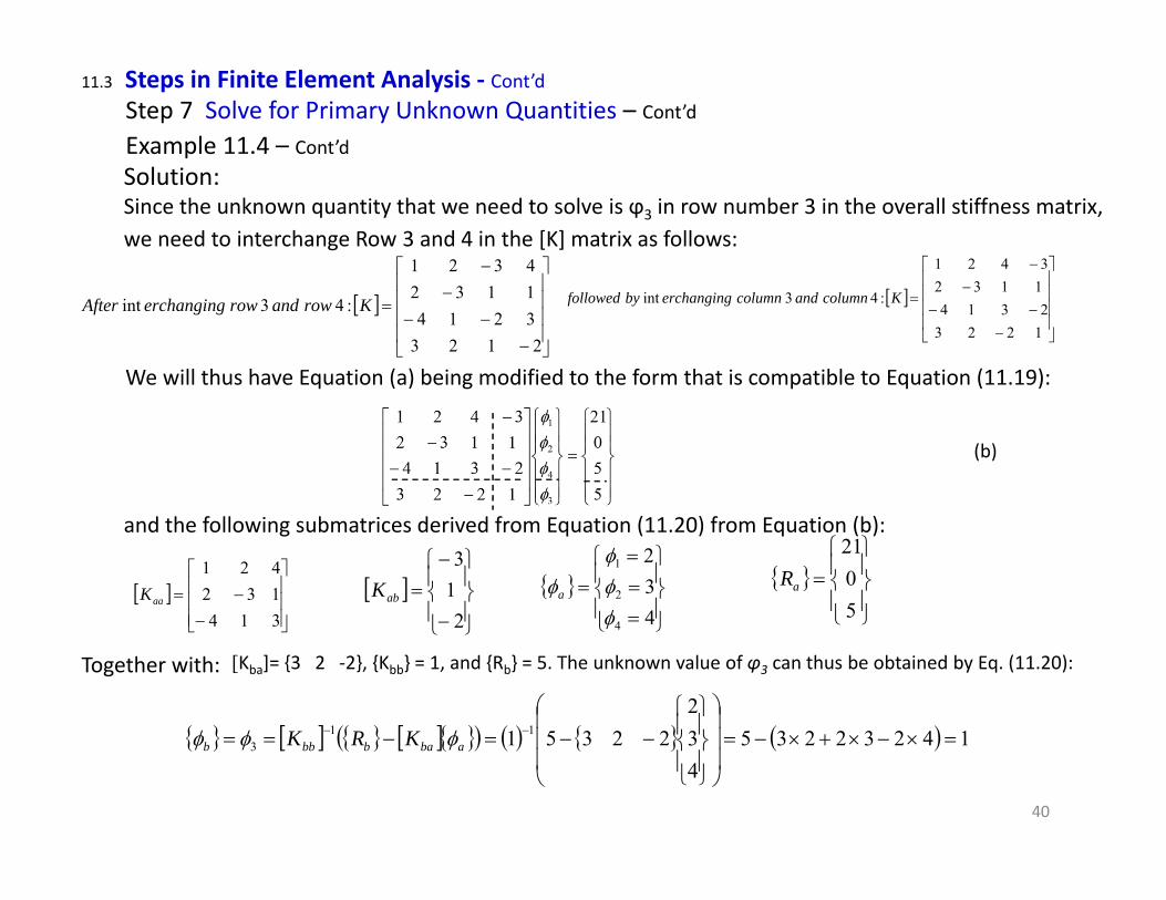
Example 11.4 – Cont’dSolution:Since the unknown quantity that we need to solve is ϕ3 in row number 3 in the overall stiffness matrix, we need to interchange Row 3 and 4 in the [K] matrix as follows:

2123321411324321

:43int KrowandrowerchangingAfter

12232314

11323421

:43int Kcolumnandcolumnerchangingbyfollowed

We will thus have Equation (a) being modified to the form that is compatible to Equation (11.19):

and the following submatrices derived from Equation (11.20) from Equation (b):

(b)

314132421

aaK

213

abK

432

4

2

1

a

5021

aR

[Kba]= {3 2 ‐2}, {Kbb} = 1, and {Rb} = 5. The unknown value of φ3 can thus be obtained by Eq. (11.20):Together with:

14232235432

22351 113

ababbbb KRK

41

11.3 Steps in Finite Element Analysis ‐ Cont’dStep 8 Solve for Secondary Unknown Quantities (p.401)

Primary unknown quantity = The first, and usually the principal unknown

quantity used in the computation

We defined primary quantities in FE analysis early in Step 2 on p.382 of finite element analysis in the following way:

We also indicated that the selection of primary quantities for the analysis may vary from case to case.

Selection of primary unknown quantities for FE analyses in mechanical and aerospace engineering include:(1) Element displacements {U}T in stress analysis, (2) Temperature {T}T for heat transfer analysis, and (3) Velocity {V}T for fluid mechanics analysis.

However, these primary unknown quantities may not be the only unknown quantities that engineers needto obtain in their problem solving. Other unknown quantities (known as Secondary Unknown Quantities) are required in many cases by the FE analyses, such as “stresses {σ}” and “strains {ε}” often are the critical quantities that engineers need to obtain in their machine structure analyses. These secondary unknown quantities can be obtained by existing formulations that relate the element displacement (the primary unknown quantity) and the “element strains” from which one may obtain the element “stress components” by using the Hooke’s law. This process of obtaining the secondary unknown quantities from the primary unknown quantities resulting from the FE analysis will be elaborated in a later Section 11.5 of this chapter. Similar procedures of computing the secondary unknown quantities from the primary unknown quantities are available from other laws of physics.

42

11.4 Output of Finite Element Analysis (p.401)

Results of outputs of the finite element analyses may take different forms. In general, these forms may include the following categories: (1) Tabulated data, (2) Contour maps of the computed unknowns in elements or nodes, (3) Different zones of both the primary and secondary unknown quantities with different color

designations over the discretized model, and (4) Visual animation of selected unknown quantities in the discretized model.

Tabulation of output may also include user’s input in material properties, descriptions of elements and nodes in the discretized model with specified boundary conditions and loadings, as illustrated in Step 1 of the finite element analysis.

There are, of course, the computed nodal displacements and stresses of all elements.

The output of element stresses by most FE codes are expressed in von‐Mises stress for multi‐axially loaded structures. Mathematical expression of von‐Mises stresses are given in Equations (11. 21a,b):

2312

322

2121 (11.21a)

where σ1, σ2 and σ3 are three principal stresses in elements.

222222 62

1xzyzxyzzxxzzyyyyxx (11.21b)

in which σxx, σyy, ….σxy, σxz, etc. are the stress components as will be define in Section11.5 (p.403).

43

11.4 Output of Finite Element Analysis - Cont’d

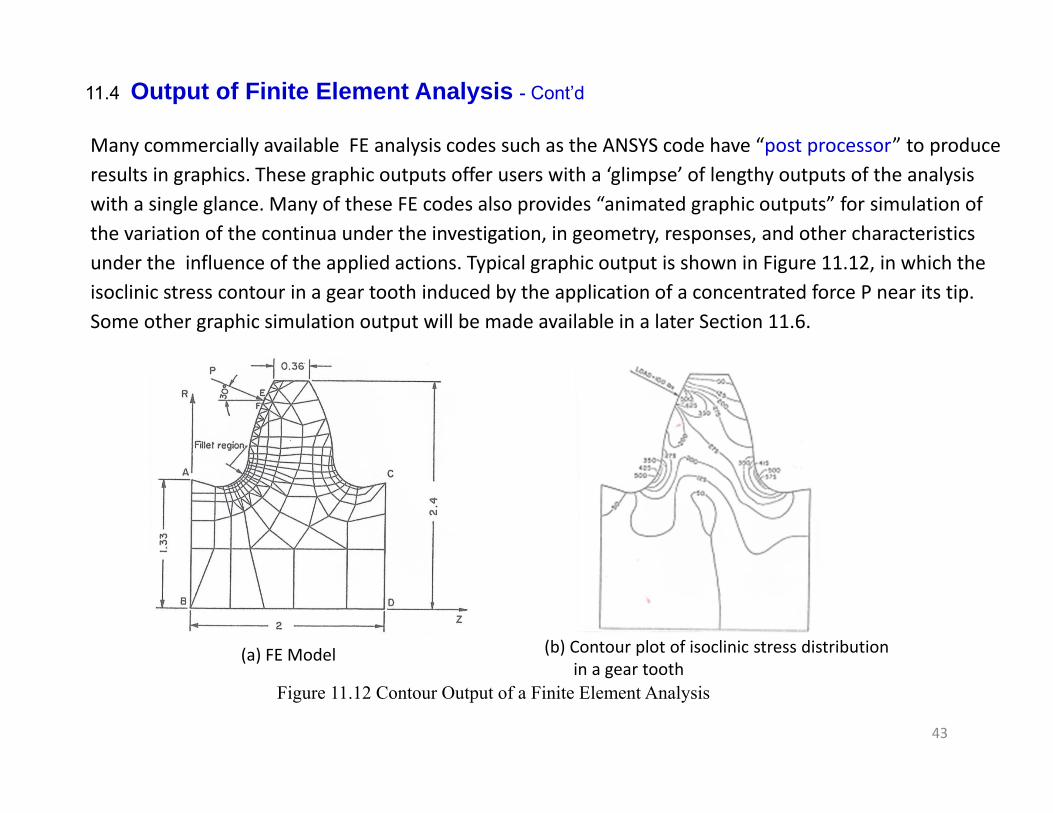
Many commercially available FE analysis codes such as the ANSYS code have “post processor” to produce results in graphics. These graphic outputs offer users with a ‘glimpse’ of lengthy outputs of the analysis with a single glance. Many of these FE codes also provides “animated graphic outputs” for simulation of the variation of the continua under the investigation, in geometry, responses, and other characteristics under the influence of the applied actions. Typical graphic output is shown in Figure 11.12, in which the isoclinic stress contour in a gear tooth induced by the application of a concentrated force P near its tip. Some other graphic simulation output will be made available in a later Section 11.6.

(a) FE Model (b) Contour plot of isoclinic stress distribution in a gear tooth

Figure 11.12 Contour Output of a Finite Element Analysis

44

11.5 Elastic Stress Analysis of Solid Structures by the FE Method (p.403)

One of the major challenges of mechanical engineers is to ensure structural integrity of machines orengineering systems that they are involved with in their professional activities. These structures can be as simple as coat hangers in Example 1.1 (p.10), and it can be as complicated as the structures of commercial airliners in Figures 1.2 (p.5) and military aircraft in Figure 3.41 (p.117) and beyond.

Structure integrity of machines or engineering systems are assessed by stress analysis using theoriesof linear elasticity, thermoelastoplasticity, and the coupled thermoelastoplasticity‐creep‐fracture mechanics.Some special‐ and general‐purpose commercially FE codes have such capabilities in advanced analysis.

In this section, we will present only the key formulation for computing induced deformation and stresses in solid structures by externally applied forces. All formulations are derived on the theory of elasticity –meaning that the deformation of the structure materialis limited within its elastic limit as stipulated in the tensile strength of the materials depicted in the Stress vs.Strain diagram shown in the right figure for common metallic materials.

45

11.5 Elastic Stress Analysis of Solid Structures by the FE Method – Cont’d

11.5.1 Stresses ‐ How does it happen (p.404)Following are 2 likely physical responses that can occur in a homogeneous solid subjected to a set of applied forces {P} as illustrated in Figure 11.14(a):

(1) the solid deforms into a new shape, and (2) the solid develops internal resistance to the

applied forces.

The induced internal resistance by the solid eventually reaches a new state of equilibrium with the applied forces, and the solid ceases further deformation under this new equilibrium condition. (a) Solid subjected to external loads

(b) Stress components in an infinitesimally small cube in deformed solid

Figure 11.14 Induced stresses in a deformed solid

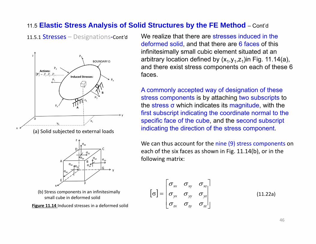
Let us consider an infinitesimally small cubic element located at (x1, y1, z1) within the deformed solid, and with its edges parallel to the three coordinates as shown in Figure 11.14(a). We envisage that there are six faces of this infinitesimally small cubic element, and there exist stress components with some normal to the faces of the cube, and some others on the faces, as shown in Figure 11.14(b).

46

We realize that there are stresses induced in the deformed solid, and that there are 6 faces of this infinitesimally small cubic element situated at an arbitrary location defined by (x1,y1,z1)in Fig. 11.14(a), and there exist stress components on each of these 6 faces.

A commonly accepted way of designation of these stress components is by attaching two subscripts to the stress σ which indicates its magnitude, with the first subscript indicating the coordinate normal to the specific face of the cube, and the second subscript indicating the direction of the stress component.

We can thus account for the nine (9) stress components on each of the six faces as shown in Fig. 11.14(b), or in the following matrix:


11.5.1 Stresses – Designations‐Cont’d

(a) Solid subjected to external loads

(b) Stress components in an infinitesimally small cube in deformed solid

Figure 11.14 Induced stresses in a deformed solid

zzzyzx

yzyyyx

xzxyxx

σ (11.22a)

47

where σxx, σyy and σzz are the stress components that exist on the faces perpendicular to the respective x-, y- and z-coordinates, and orient along the same respective coordinates. We will call these stress components the “normal stresses” in the deformed solid.

The other 6 stress components with different subscripts, such as σxy and σxz, etc. are called shearing stress components,( with σxy exists on the cube face that is normal to the x-coordinate and points in the y-direction and σxz being another shearing stress existing on the same cube face but points to the z-directiotn).


11.5.1 Stresses – 6 independent stress components ‐ Cont’dWe have designated 9 induced stress components existing on each of the 6 faces of a point inside an deformed solid at (x,y,z) representedby an infinitesimally small cube, by a square matrix:

zzzyzx

yzyyyx

xzxyxx

σ (11.22a)

Due to the fact the 9 stresses on the 6 faces of the cube in in full equilibrium under the deformed state, this number is reduced to six in Equation (11.22b) with the relationships of: σxy = σyx, σyz = σzy and σxz = σzx. We thus have the 6 independent stress components in deformed solid in three-dimensional stress analyses:

zz

yzyy

xzxyxx

SYM

(11.22b)

48


11.5.2 Displacements (p.406)Displacements in a deformed solid means the change of shape of the solid due to externally applied forces as illustrated in Figure 11.15

Displacement of the solid may be mathematically expressed by the net movement of Point P1 to P2 , and it can be represented by a vector U with components u, v and w along the coordinates x, y and z respectively.

The displacement vector of a point P located in (x,y,z) can thus be expressed as:

, , =, ,

, , , ,

(11.24)

where u(x,y,z), v(x,y,z) and w(x,y,z) are the components of the displacement in element locatedat (x,y,z) in a deformed solid along the x‐, y‐ and z‐coordinate respectively.

Figure 11.15 Displacements in a Deformed Solid

49


11.5.3 Strains (p.406)

Figure 11.15 Displacements in a Deformed Solid

Figure 11.15 illustrates the change of the shape of a solid as a result of the applied forces {P}. This change of shape of the solid ceases after the solid reaches a new equilibrium of its state with induced resistance by the material and the change of the shape of the solid.We may observe that the “intensity” of these resistances in terms of “stresses” existing everywhere in the deformed solid, including at Point P(x,y,z) in Figure 11.15, and the stresses at this “point” (now represented by an infinitesimally small cube) as shown in Figure 11.14(b)

Figure 11.14(b)

One may envisage that these stresses appearing on the faces of the cube would have also caused the changes in either the “size” or the“shape” of the cube from its original state to the current state of the induced deformation.

If we express the 6 independent stress components in Equation (11.22b) into a column matrix in the following form:

654321 T (11.23)

in which σ1 = σxx σ2 = σyy σ3 = σzz σ4 = σxy σ5 = σyz σ6 = σxz shown in Figure 11.14(b)

We may also express the corresponding 6 strain components in a similar form: 654321 T (11.25)

with ϵ1 = ϵxx ϵ2 = ϵyy ϵ3 = ϵzz ϵ4 = ϵxy ϵ5 = ϵyz ϵ6 = ϵxz

50


11.5.4 Fundamental Relationships in Linear Elasticity (p.407) In this sub‐section, we will outline the relationships of the three essential physical quantities of stresses {σ}, strains {ε} and displacements {u} in stress analysis of solid structures. These relationships were derived by the theory of elasticity. We will only present these formulations that are relevant to the subsequent derivations of equations and formula required for the subsequent finite element analysis.

11.5.4.1 Strain‐displacement relations (p.407):We designated displacements of the deformed solid by {U(x,y,z)} from Point P1 at (x,y,z) to Point P2 at (x+u, y+v, z+w) as in Figure 11.15, with:u = u(x,y,z) for the net movement of the point along the x‐coordinate, v = v(x,y,z) to be the net movement of the same point along the

y‐coordinate w= w(x,y,z) to be the net movement of the point along the z‐coordinate.

Displacements represent variation in LINEAR dimensions. Strains in the deformed solid are measures of the “rate” of changes of linear dimensions of a solid located at (x,y,z) represented by a cube in Figure 11.14(b) over its original linear dimensions. By referring to the cubic in Figure 11.14(b), the corresponding strain component εxxassociated with normal stress component σxx along the x‐coordinate can be related to be: εxx=ΔAD/AD, in which ΔAD is the change of the length of the side AD due to the action of stress σxx. It is logical to say that the normal strains that are associated with normal stresses result in the linear dimensional change of the solid, or we may conclude that the 3 normal strains components represent “dimensional change of the solid.”

Figure 11.15

Figure 11.14(b)

51


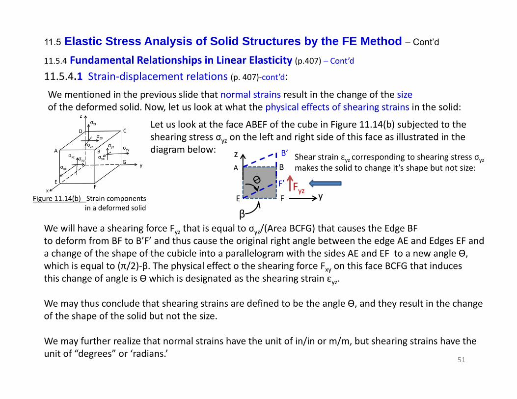
11.5.4 Fundamental Relationships in Linear Elasticity (p.407) – Cont’d 11.5.4.1 Strain‐displacement relations (p. 407)‐cont’d:We mentioned in the previous slide that normal strains result in the change of the sizeof the deformed solid. Now, let us look at what the physical effects of shearing strains in the solid:

Let us look at the face ABEF of the cube in Figure 11.14(b) subjected to the shearing stress σyz on the left and right side of this face as illustrated in the diagram below:

Fyz

A B

E F

B’

F’y

z

βWe will have a shearing force Fyz that is equal to σyz/(Area BCFG) that causes the Edge BF to deform from BF to B’F’ and thus cause the original right angle between the edge AE and Edges EF and a change of the shape of the cubicle into a parallelogram with the sides AE and EF to a new angle ϴ, which is equal to (π/2)‐β. The physical effect o the shearing force Fxy on this face BCFG that induces this change of angle is ϴ which is designated as the shearing strain εyz.

We may thus conclude that shearing strains are defined to be the angle ϴ, and they result in the change of the shape of the solid but not the size.

We may further realize that normal strains have the unit of in/in or m/m, but shearing strains have the unit of “degrees” or ‘radians.’

Figure 11.14(b) Strain components in a deformed solid

Shear strain εyz corresponding to shearing stress σyzmakes the solid to change it’s shape but not size:

52


11.5.4 Fundamental Relationships in Linear Elasticity – Cont’d 11.5.4.1 Strain‐displacement relations (p.407)‐cont’d:

We may thus relate the strain and displacement relations in the following expressions:

x

zyxuzyxxx

,,,,

y

zyxvzyxyy

,,,,

z

zyxwzyxzz

,,,,

y

zyxux

zyxvzyxxy

,,,,,,

z

zyxvy

zyxwzyxyz

,,,,,,

z

zyxux

zyxwzyxxz

,,,,,,

(A) 3 independent normal strain components:

(B) 3 independent shearing strain components:

(11.26a)

(11.26b)

(11.26c)

(11.26d)

(11.26e)

(11.26f)

53


11.5.4 Fundamental Relationships in Linear Elasticity – Cont’d 11.5.4.1 Strain‐displacement relations‐cont’d:

The relationships in Equations (11.26a to f) may be expressed in the following matrix form:

zyxwzyxvzyxu

xz

yz

xy

z

y

x

xz

yz

xy

zz

yy

xx

,,,,,,

0

0

0

00

00

00

(11.27)

or in the following form Equation (11.28) for the subsequent derivation of element equations:

zyxwzyxvzyxu

xz

yz

xy

z

y

x

xz

yz

xy

zz

yy

xx

,,,,,,

0

0

0

00

00

00

(11.27)

UD (11.28)

where

xz

yz

xy

z

y

x

D

0

0

0

00

00

00

(11.29)

54


11.5.4 Fundamental Relationships in Linear Elasticity – Cont’d 11.5.4.2 Stress‐Strain relations (p.408):We will refer to the stress components in Figure 11.14 (b) to relate the corresponding strain components using the generalized Hooke’s law inthe following forms:

xz

yz

xy

zz

yy

xx

xz

yz

xy

zz

yy

xx

SYM

E

221

0221

00221

000100010001

211

(11.30)

or in a compact form: C (11.31)

where E is the Young’s modulus and ν is the Poisson’s ratio of the material.

The matrix [C], called elasticity matrix has the form:

221

0221

00221

000100010001

211

SYM

EC (11.32)

Figure 11.14(b)

55


11.5.4 Fundamental Relationships in Linear Elasticity – Cont’d 11.5.4.3 Strain Energy in Deformed Elastic Solids (p.409):

The above formulations are derived on a postulation that a deformed solid elastic solids with induced deformations (or displacements) {U}, stresses {σ} and strains {ε} by applied external forces in an equilibrium state will disappear altogether after the removal of the applied forces.

This postulation leads us to believe that there must be a mechanism that restores the solid to its original state after the removal of the applied loads.

This mechanism is referred to as the “strain energy.”

This energy is induced in the solid during the deformation process, and it is “stored” in the deformed solid at the equilibrium under the external loading. It will be released to restore the deformed solid to its original state after the removal of the applied actions.

56


11.5.4 Fundamental Relationships in Linear Elasticity – Cont’d 11.5.4.3 Strain Energy in Deformed Elastic Solids (p.409) ‐ Cont’d:

dvUv

yzyzxzxzxyxyzzzzyyyyxxxx 21,

dvUv

T 21,

Since the energy to restore the size and shape of the solid once the externally applied forces are removed is created by the deformation of the solid as expressed by the strains induced by the externally applied forces associated with the induced stresses, we may mathematically express this energy in the following form:

where v is the volume of the solid, or in a compact form:

(11.33)

(11.34)

57


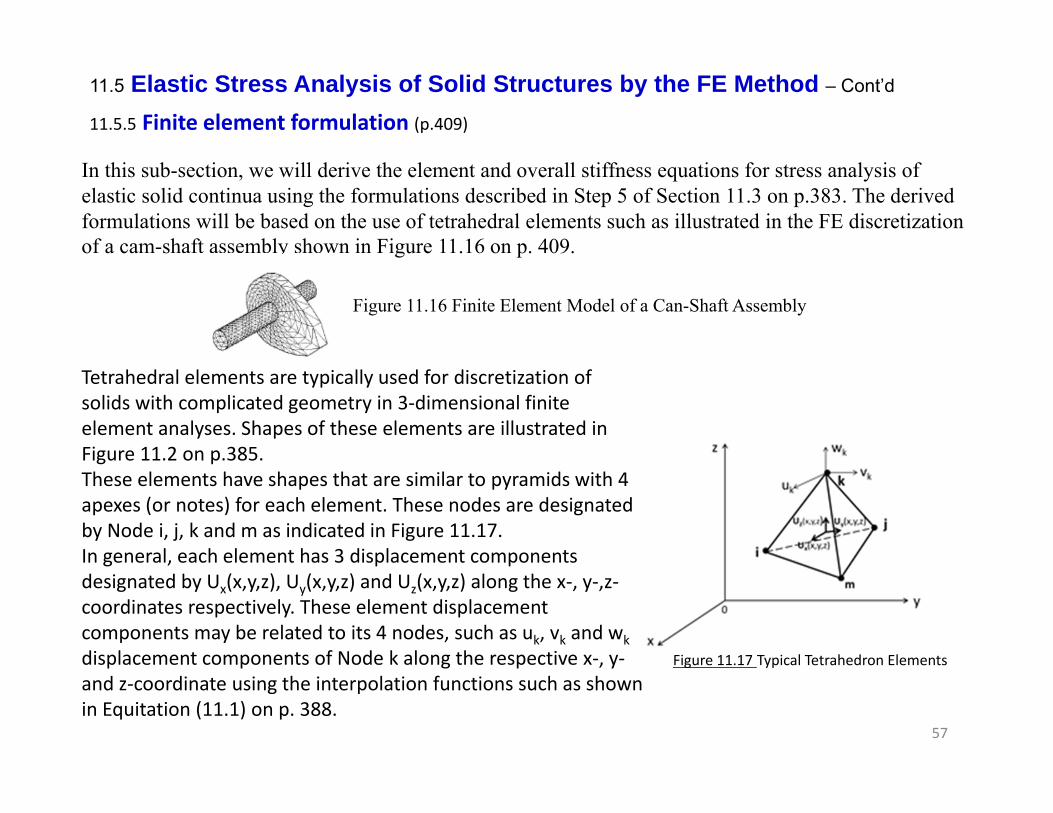
11.5.5 Finite element formulation (p.409)

In this sub-section, we will derive the element and overall stiffness equations for stress analysis of elastic solid continua using the formulations described in Step 5 of Section 11.3 on p.383. The derived formulations will be based on the use of tetrahedral elements such as illustrated in the FE discretization of a cam-shaft assembly shown in Figure 11.16 on p. 409.

Figure 11.16 Finite Element Model of a Can-Shaft Assembly

Tetrahedral elements are typically used for discretization of solids with complicated geometry in 3‐dimensional finite element analyses. Shapes of these elements are illustrated in Figure 11.2 on p.385.These elements have shapes that are similar to pyramids with 4 apexes (or notes) for each element. These nodes are designated by Node i, j, k and m as indicated in Figure 11.17. In general, each element has 3 displacement components designated by Ux(x,y,z), Uy(x,y,z) and Uz(x,y,z) along the x‐, y‐,z‐coordinates respectively. These element displacement components may be related to its 4 nodes, such as uk, vk and wkdisplacement components of Node k along the respective x‐, y‐and z‐coordinate using the interpolation functions such as shown in Equitation (11.1) on p. 388.

Figure 11.17 Typical Tetrahedron Elements

58


11.5.5 Finite element formulation – Cont’d

zyxzyxzyx

zyxzyxzyx

zyx,,W,,V,,U

,,U,,U,,U

,,U

z

y

x

We begin our formulation by expressing the element displacement and its components in the form:

where U(x,y,z), V(x,y,z) and W(x,y,z) are the components of element displacement along x‐, y‐and z‐coordinates respectively in a rectangular coordinate system.

We may also express the Element displacements {U(x,y,z)} in terms of the components at its associated Nodes, {u} using the interpolation function [N(x,y,z)] in Equation (11.1) to give:

u,,,,U,,U,,U

,,U

z

y

x

zyxNzyxzyxzyx

zyx

(11.35)

The displacement components {u} in Equation (11.35) for all 4 nodes in the tetrahedral element in Figure 11.17are designated as follows:{u}T = {ui vi wi} for Node i,

= {ui vj wj} for Node j,= {uk vk wk} for Node k (as shown in Fig.11.17)= {um vm wm} for Node m


59


11.5.5 Finite element formulation (p.411) – Cont’d


These nodal displacements at the 4 nodes are point values with real numbers. The total number of displacement components of the four nodes of a tetrahedral element in Figure 11.17 is thus equal to 12, as expressed in the following matrix form:

mmmkkkjjjiiiT wvuwvuwvuwvuu (11.36)

We may thus express the Element displacements in the tetrahedral element in Figure 11.17 in terms of The displacements of its 4 nodes by the flowing expression:

u,,,,,,),,(u,,,,U,,U,,U

,,U

z

y

x

zyxNzyxNzyxNzyxNzyxNzyxzyxzyx

zyx mkji

(11.37)

or, in a compact form: mkji uuuu,,U mkji NNNNzyx

where Ni, Nj, Nk and Nm are the components of the interpolation function associated with Node i, j, k and m in Figure 11.17 respectively.

60


11.5.5 Finite element formulation (p.411) – Cont’d

We will then derive the expression for the strains in the element in terms of the nodal displacements by substituting Equation (11.35) into Equation (11.28) and obtain:

uzyxBzyx ..,, (11.38)where the matrix [B] has the form:

zyxNDzyxB ,,),,( (11.39)

The matrix [B(x,y,z)] in Equation (11.39) may be obtained by the derivatives of [N(x,y,z)] with respect to the coordinates x-, y- and z- respectively. The matrix [D] is given in Equation (11.29) on p.408.

The element stresses in terms of nodal displacement components are related by substituting Equation (11.38) into Equation (11.31) on p.408 to give:

uzyxBCzyx ,,,, (11.40)

And finally, the expression of strain energy in the deformed element is obtained by substituting Equations (11.38) and (11.40) into Equation (11.34) on p.409, resulting in the following equation for the strain energy of the deformed element:

dvuzyxBCzyxBuuUv

TT ..,,21 (11.41)

The strain energy U({u}) in Equation (11.41) is the energy stored in the deformed solid (elements in this case). It is induced by the applied forces at the nodes of the elements.

61

11.5 Elastic Stress Analysis of Solid Structures by the FE Method – Cont’d11.5.5 Finite element formulation – derivation of Element equations (p.412)

In Step 5 of Section 11.3 (p.394), we presented the element equations for discretized continua given in Equation (11.17) on p.396: , in which [Ke]=the element stiffness matrix, {φ} = nodal quantities (e.g., displacements of the same element). Element equations are then used to derive the overall stiffness equation in Equation (11.18) on p. 397 with the overall stiffness matrix [K] = where M=total number of elements in the discretized model used in FE analysis, and {R} is the column matrix that accounts for the net forces on every node of the discretized continuum. Further, we learned that element equations are derived by either Rayleigh‐Ritz method on p.394 with identifiable functionals (χ), or by the Galerkinmethod (p.395) with identifiable differential equations.

FKe

RK M

eK

We will use the Rayleigh‐Ritz variation method (p. 394) to derive the element equations for the present case of elastic stress analysis of a solid loaded by applied forces {P} on it surface as illustrated in Figure 11.1. Figure 11.2 is the discretized model of the same loaded solid. The reason for us using this method is becausethere is no identifiable differential equations that can describe the present case as required by the Galerkinmethod. Our effort in using the Rayleigh‐Ritz method in deriving the element equation is to derive a suitable functional that is suitable for the present case and situation.

Fig. 11.1 A continuum subject to Applied Forces {P(r)}Fig. 11.2 FE discretization of a continuum subject to forces

62


11.5.5 Finite element formulation – derivation of Element equations (p.412) ‐ Cont’d

Fig. 11.1 A continuum subject to Applied Forces {P(r)} Fig. 11.15 Induced deformation of a

continuum applied forces

We will derive the element equation similar to Equation (11.17) on p.396 and then the overall stiffness equation of the entire structure similar to Equation (11.18) on p.397. The principle of deriving the Element equation for the FE analysis of deformed elastic solids will be based on the following observations on the Figures 11.1, 11.15 and 11.14(b) appeared on the top of this slide:

(1) We have an elastic solid continuum subject to a set of forces applied at its surface as illustrated inFigure 11.1

(2) The above situation results in two responses by the solid continuum: (a) it deforms from the shape of the continuum into a new shape from the solid curve to that in dotted curve in Figure 11.15, and (b) there is internal resistance generated simultaneously with its deformation. We realize that the solid deformation is represented by “Strains” in the continuum, and the resistance is represented by stresses with components illustrated by what is shown in Figure 11.14,

(3) We view the deformation in the solid continuum created by the applied forces as the “work” done byapplied forces to the deformed continuum, Wp.

63

11.5 Elastic Stress Analysis of Solid Structures by the FE Method – Cont’d11.5.5 Finite element formulation – derivation of Element equations ‐ Cont’d

Fig. 11.1 A continuum subject to Applied Forces {P(r)}

Fig. 11.15 Induced deformation of a continuum applied forces

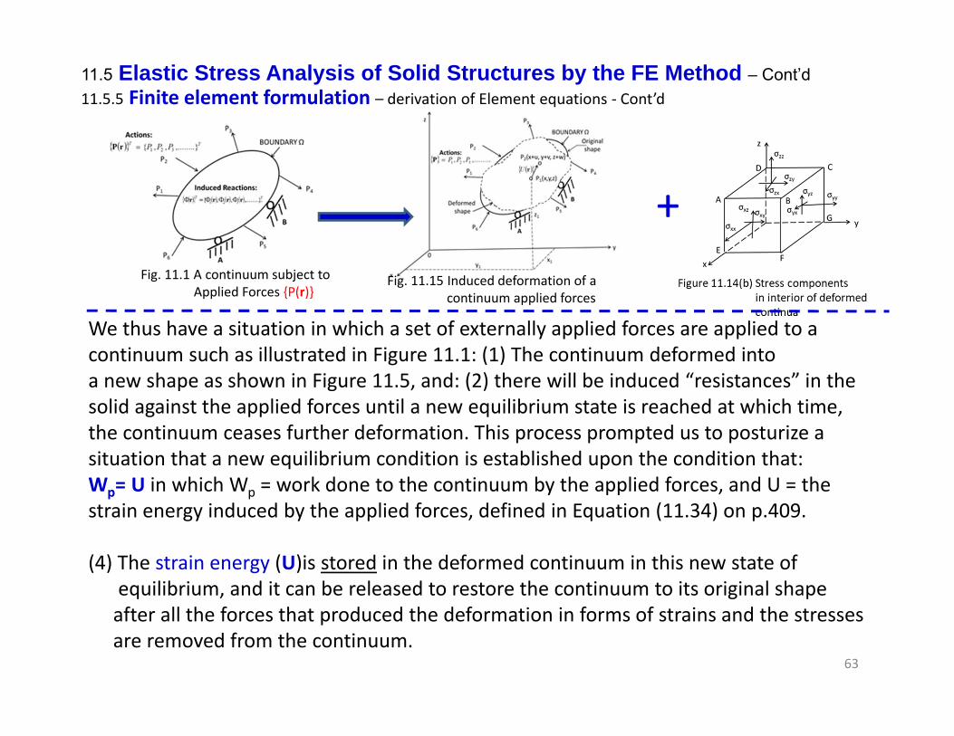
We thus have a situation in which a set of externally applied forces are applied to a continuum such as illustrated in Figure 11.1: (1) The continuum deformed intoa new shape as shown in Figure 11.5, and: (2) there will be induced “resistances” in the solid against the applied forces until a new equilibrium state is reached at which time, the continuum ceases further deformation. This process prompted us to posturize a situation that a new equilibrium condition is established upon the condition that:Wp= U in which Wp = work done to the continuum by the applied forces, and U = the strain energy induced by the applied forces, defined in Equation (11.34) on p.409.

(4) The strain energy (U)is stored in the deformed continuum in this new state of equilibrium, and it can be released to restore the continuum to its original shape after all the forces that produced the deformation in forms of strains and the stresses are removed from the continuum.

64


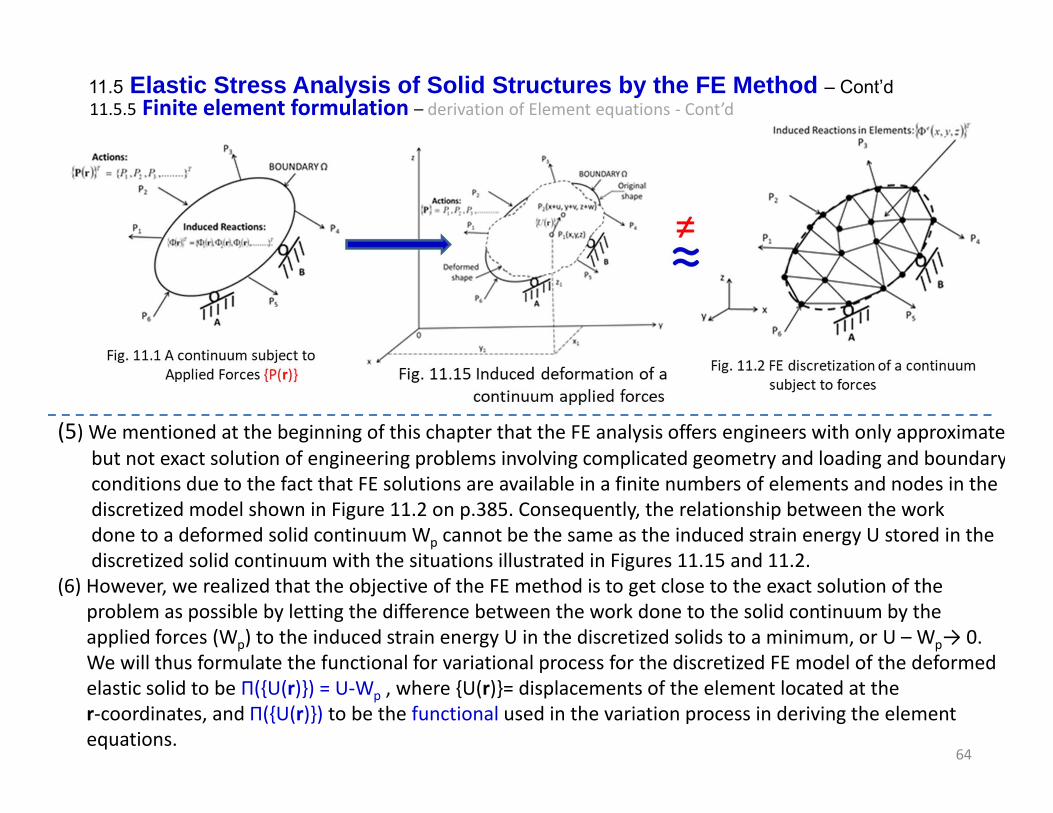
(5) We mentioned at the beginning of this chapter that the FE analysis offers engineers with only approximatebut not exact solution of engineering problems involving complicated geometry and loading and boundaryconditions due to the fact that FE solutions are available in a finite numbers of elements and nodes in the discretized model shown in Figure 11.2 on p.385. Consequently, the relationship between the work done to a deformed solid continuum Wp cannot be the same as the induced strain energy U stored in the discretized solid continuum with the situations illustrated in Figures 11.15 and 11.2.

(6) However, we realized that the objective of the FE method is to get close to the exact solution of the problem as possible by letting the difference between the work done to the solid continuum by the applied forces (Wp) to the induced strain energy U in the discretized solids to a minimum, or U – Wp→ 0. We will thus formulate the functional for variational process for the discretized FE model of the deformed elastic solid to be Π({U(r)}) = U‐Wp , where {U(r)}= displacements of the element located at the r‐coordinates, and Π({U(r)}) to be the functional used in the variation process in deriving the element equations.

65


Π({U(r)}) = U‐Wp

We have derived the functional for variation in deriving the element equation for an elastically deformed element in the form: . However, in view that all elements in discretized FE models are interconnected at nodes, we will express this functional in terms of nodal displacement components vis. the interpolation function N(x,y,z) in a rectangular coordinate system. We will have the Functional expressed in such a way:

Πwhere U({u}) = strain energy of the element in terms of nodal displacements {u}, and the work done to the element by the applied forces has the form of:

dstzyxUdvfzyxUWT

s

T

vp ,,,,

in which U(x,y,z) are the components of displacement of the element, {f} are the body forces, such as the weight or dynamic forces of the element, and {t} are the “surface tractions” such as pressure orother forms of forces applied on the edges of the element. We have already derived the expression of the strain energy shown in Equation (11.41):

dvuzyxBCzyxBuuUv

TT ..,,21 (11.41)

The functional (or strain energy) in the element can thus be expressed in terms of nodal displacement with the interpolation function [N(x,y,z)] in the following expression:

dstzyxNudvfzyxNu

dvuzyxBCzyxBuu

TT

s

TT

v

v

TT

,,,,

..,,21

(11.42)

One may readily realize that Π({u}) in Equation (11.42) also represent the potential energy that is“stored” in the deformed element in a equilibrium condition.

66


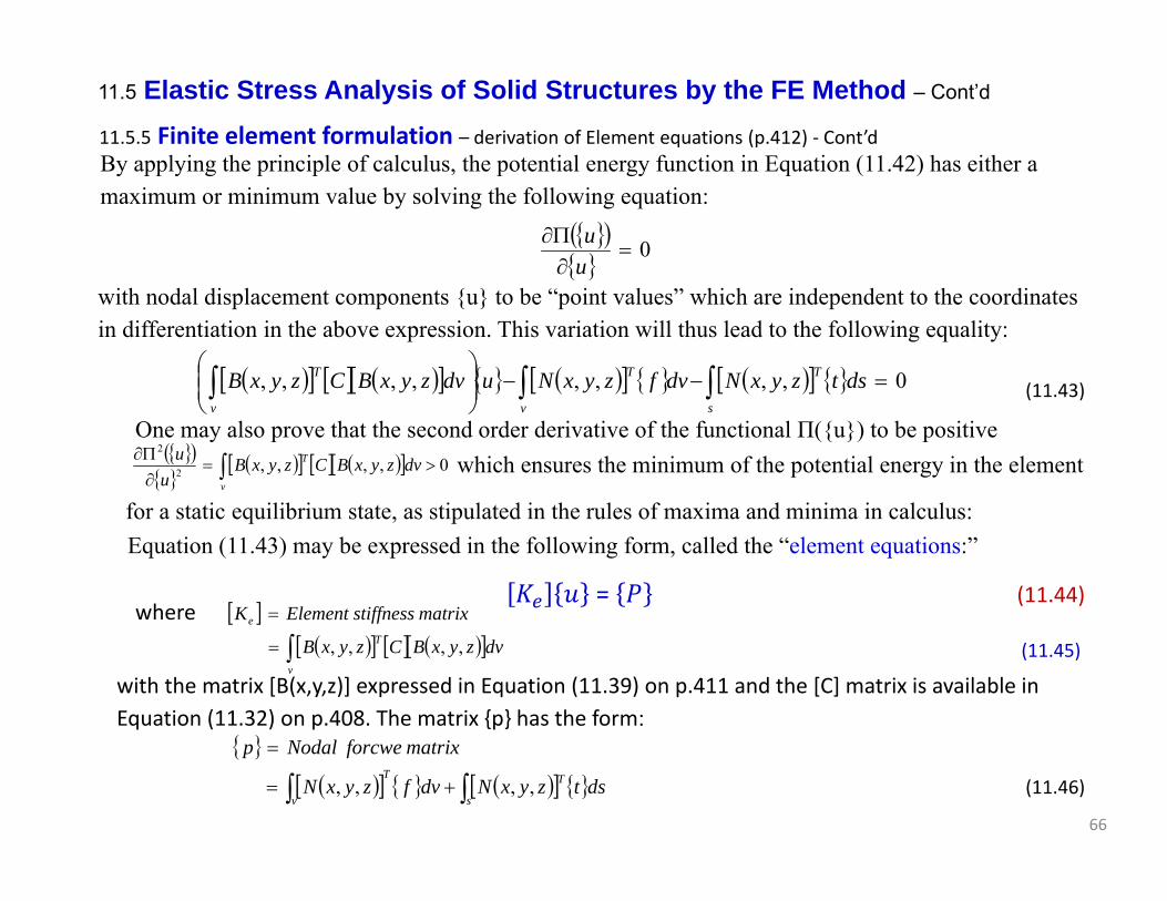
11.5.5 Finite element formulation – derivation of Element equations (p.412) ‐ Cont’d By applying the principle of calculus, the potential energy function in Equation (11.42) has either a maximum or minimum value by solving the following equation:

0

uu

with nodal displacement components {u} to be “point values” which are independent to the coordinates in differentiation in the above expression. This variation will thus lead to the following equality:

0,,,,,,,,

dstzyxNdvfzyxNudvzyxBCzyxBs

T

v

T

v

T(11.43)

One may also prove that the second order derivative of the functional Π({u}) to be positive

Equation (11.43) may be expressed in the following form, called the “element equations:”

0,,,,2

2

v

T dvzyxBCzyxBu

u which ensures the minimum of the potential energy in the element

for a static equilibrium state, as stipulated in the rules of maxima and minima in calculus:

= (11.44)

dvzyxBCzyxB

matrixstiffnessElementK

v

T

e

,,,,

where

(11.45)

with the matrix [B(x,y,z)] expressed in Equation (11.39) on p.411 and the [C] matrix is available in Equation (11.32) on p.408. The matrix {p} has the form:

dstzyxNdvfzyxN

matrixforcweNodalp

s

TT

v

,,,, (11.46)

67


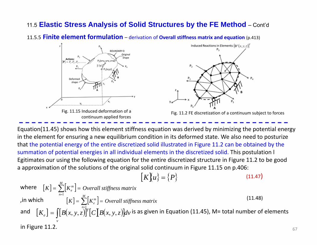
11.5.5 Finite element formulation – derivation of Overall stiffness matrix and equation (p.413)

Fig. 11.2 FE discretization of a continuum subject to forcesFig. 11.15 Induced deformation of a continuum applied forces

Equation(11.45) shows how this element stiffness equation was derived by minimizing the potential energyin the element for ensuring a new equilibrium condition in its deformed state. We also need to posturize that the potential energy of the entire discretized solid illustrated in Figure 11.2 can be obtained by thesummation of potential energies in all individual elements in the discretized solid. This postulation lEgitimates our using the following equation for the entire discretized structure in Figure 11.2 to be gooda approximation of the solutions of the original solid continuum in Figure 11.15 on p.406:

PuK (11.47)

matrixstiffnessOverallKKM

n

me

1

where

matrixstiffnessOverallKKM

n

me

1

,in which (11.48)

dvzyxBCzyxBKv

Te ,,,,and is as given in Equation (11.45), M= total number of elements

in Figure 11.2.

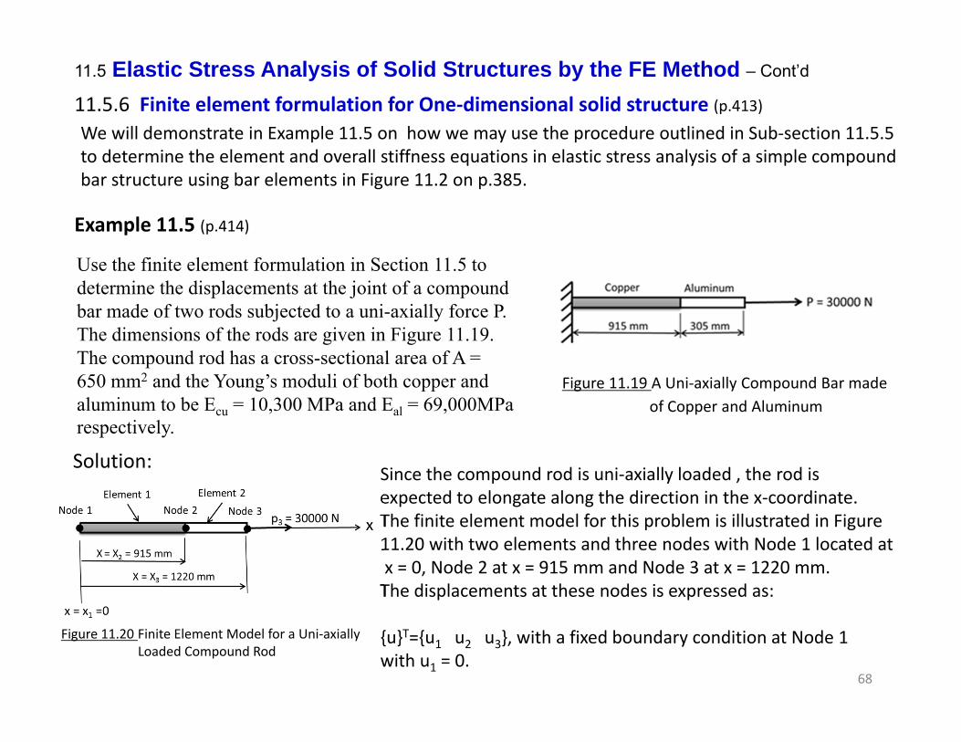
68


11.5.6 Finite element formulation for One‐dimensional solid structure (p.413) We will demonstrate in Example 11.5 on how we may use the procedure outlined in Sub‐section 11.5.5to determine the element and overall stiffness equations in elastic stress analysis of a simple compound bar structure using bar elements in Figure 11.2 on p.385.

Example 11.5 (p.414)

Use the finite element formulation in Section 11.5 to determine the displacements at the joint of a compound bar made of two rods subjected to a uni-axially force P. The dimensions of the rods are given in Figure 11.19. The compound rod has a cross-sectional area of A = 650 mm2 and the Young’s moduli of both copper and aluminum to be Ecu = 10,300 MPa and Eal = 69,000MPa respectively.

Figure 11.19 A Uni‐axially Compound Bar made of Copper and Aluminum

Solution:Since the compound rod is uni‐axially loaded , the rod is expected to elongate along the direction in the x‐coordinate. The finite element model for this problem is illustrated in Figure 11.20 with two elements and three nodes with Node 1 located atx = 0, Node 2 at x = 915 mm and Node 3 at x = 1220 mm. The displacements at these nodes is expressed as:

{u}T={u1 u2 u3}, with a fixed boundary condition at Node 1 with u1 = 0.

Figure 11.20 Finite Element Model for a Uni‐axiallyLoaded Compound Rod

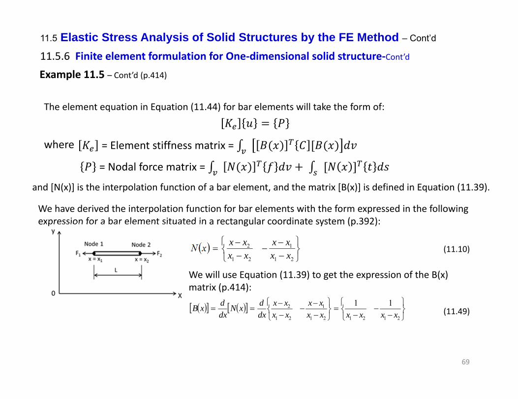
69


11.5.6 Finite element formulation for One‐dimensional solid structure‐Cont’dExample 11.5 – Cont’d (p.414)

The element equation in Equation (11.44) for bar elements will take the form of:

where = Element stiffness matrix =

and [N(x)] is the interpolation function of a bar element, and the matrix [B(x)] is defined in Equation (11.39).

= Nodal force matrix =

We have derived the interpolation function for bar elements with the form expressed in the followingexpression for a bar element situated in a rectangular coordinate system (p.392):

21

1

21

2

xxxx

xxxxxN (11.10)

We will use Equation (11.39) to get the expression of the B(x) matrix (p.414):

212121

1

21

2 11xxxxxx

xxxxxx

dxdxN

dxdxB (11.49)

70

By substituting the above expression of [N(x)] in Equation (11.10), [B(x)] in Equation (11.49), and with [C] = E and dv=Adx with A being the cross-sectional area of the bar element and x1-x2 = -L into Equations (11.42) and (11.43), we will obtain the element stiffness matrix from Equation (11.45):


11.5.6 Finite element formulation for One‐dimensional solid structure‐Cont’dExample 11.5 – Cont’d

11

1111110 L

EAAdxLL

ELL

KL

T

e (11.50)

The nodal forces matrix to a uni-axially loaded bar element is: {p}T = {-F1 F2}The element equation of the bar element thus has the form from Equation (11.44) to be:

2

1

2

1

1111

FF

uu

LEA (11.51)

mNxxx

LAEKe /10

317.7317.7317.7317.7

1111

1091565010300

1111 6

31

111

Our current analysis involves 2 elastic bars with dimensions shown in Figure 11.20. We may establish both element equations by using Equation (11.51) with the following data:

Element No. Length (L),mm

Young’s modulus (E), MPa

1 L1=915 E1=10300

2 L2=305 E2=69000

(a)

mNxx

xLAEKe /10

05.14705.14705.14705.147

1111

1030565069000

1111 6

32

222

(b)

A=650 mm2

71


11.5.6 Finite element formulation for One‐dimensional solid structure‐Cont’dExample 11.5 – Cont’d on overall stiffness equation and solution (p.415):

mNxxx

LAEKe /10

317.7317.7317.7317.7

1111

1091565010300

1111 6

31

111

(a)

mNxx

xLAEKe /10

05.14705.14705.14705.147

1111

1030565069000

1111 6

32

222

(b)

The element equations for both Element 1 and 2 with stiffness matrices shown in Equations (a) and (b) thus take the following forms in Equation (11.44) to give:

2

1

2

166

66

10317.710317.710317.710317.7

pp

uu

xxxx

for Element 1: (c)and

3

2

3

266

66

1005.1471005.1471005.1471005.147

pp

uu

xxxx

(d)for Element 2:

In view of the sharing of Node 2 by both the elements, the overall stiffness matrix of the structure following the rule of assembly as described in Example 11.3 and Figure 11.11 to give:

05.1470005.147367.1540

0317.7317.710

05.1470005.14705.147317.70

0317.7317.710 66K N/m (e)

We may thus use the above overall stiffness equation and the element equations in Equations (c) and (d) to obtain the overall stiffness equation of the compound bar following Equation (11.47) as:

30000000

05.1470005.147367.1540

0317.7317.710

3

2

1

3

2

16

ppp

uu

u

(f)

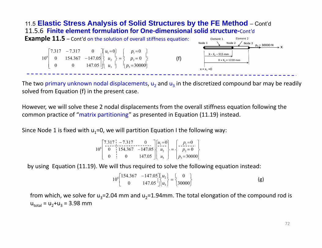
72

11.5 Elastic Stress Analysis of Solid Structures by the FE Method – Cont’d11.5.6 Finite element formulation for One‐dimensional solid structure‐Cont’dExample 11.5 – Cont’d on the solution of overall stiffness equation:

30000000

05.1470005.147367.1540

0317.7317.710

3

2

1

3

2

16

ppp

uu

u(f)

The two primary unknown nodal displacements, u2 and u3 in the discretized compound bar may be readily solved from Equation (f) in the present case.

However, we will solve these 2 nodal displacements from the overall stiffness equation following the common practice of “matrix partitioning” as presented in Equation (11.19) instead.

Since Node 1 is fixed with u1=0, we will partition Equation I the following way:

by using Equation (11.19). We will thus required to solve the following equation instead:

30000

005.147005.147367.154

103

26

uu

(g)

from which, we solve for u3=2.04 mm and u2=1.94mm. The total elongation of the compound rod isutotal = u2+u3 = 3.98 mm

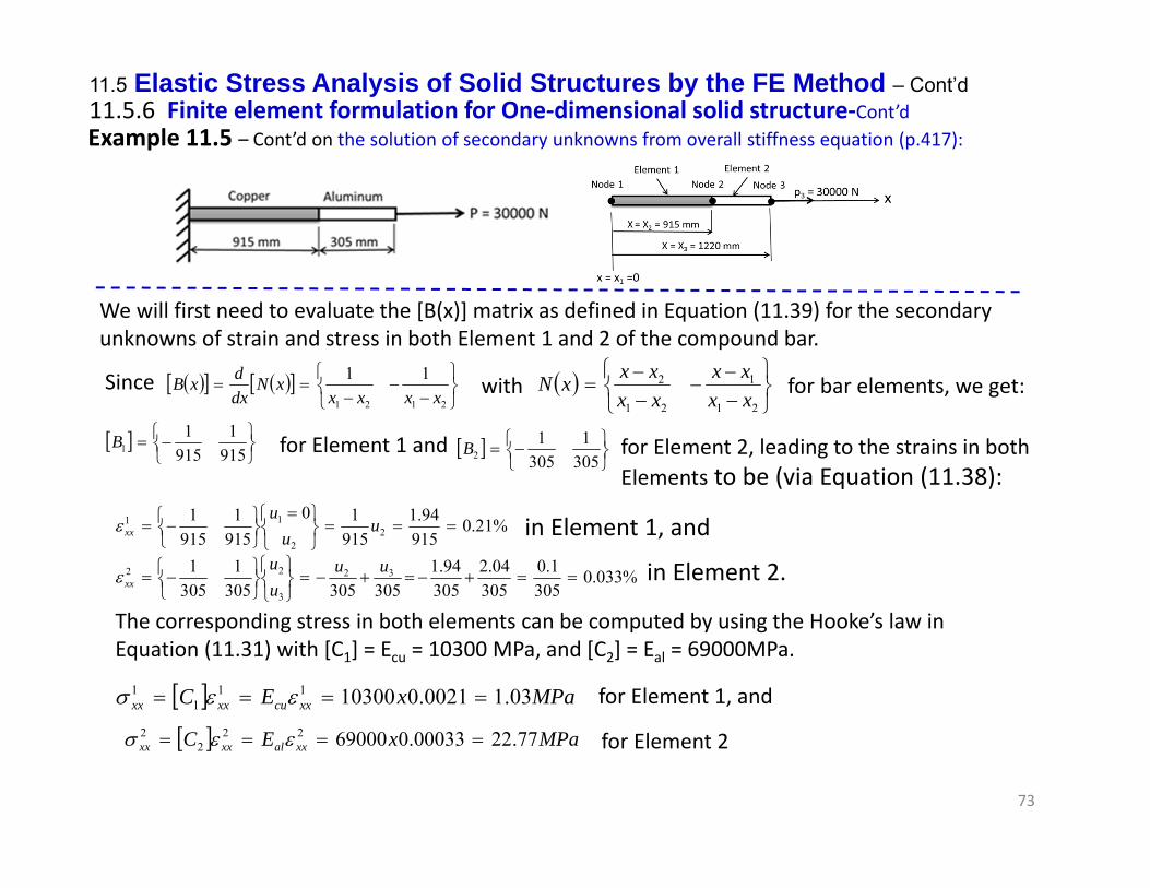
73

11.5 Elastic Stress Analysis of Solid Structures by the FE Method – Cont’d11.5.6 Finite element formulation for One‐dimensional solid structure‐Cont’dExample 11.5 – Cont’d on the solution of secondary unknowns from overall stiffness equation (p.417):

We will first need to evaluate the [B(x)] matrix as defined in Equation (11.39) for the secondary unknowns of strain and stress in both Element 1 and 2 of the compound bar.

2121

11xxxx

xNdxdxB

21

1

21

2

xxxx

xxxxxNwith for bar elements, we get:Since

9151

9151

1B for Element 1 and

3051

3051

2B for Element 2, leading to the strains in both Elements to be (via Equation (11.38):

%21.0915

94.191510

9151

9151

22

11

u

uu

xx in Element 1, and

%033.0305

1.0305

04.2305

94.1305305305

13051 32

3

22

uuuu

xx in Element 2.

The corresponding stress in both elements can be computed by using the Hooke’s law in Equation (11.31) with [C1] = Ecu = 10300 MPa, and [C2] = Eal = 69000MPa.

MPaxEC xxcuxxxx 03.10021.010300111

1 for Element 1, and

MPaxEC xxalxxxx 77.2200033.069000222

2 for Element 2

74

11.6 General‐Purpose Finite Element Analysis Codes (p.417)The incredible versatility of the finite element method coupled with the unprecedented rapid advance of digital technologies for computer hardware and software technologies has resulted in broad acceptance of this method by members of science and engineering communities in handling all sorts of problems with great accuracy and reliabilities that are much beyond the capabilities of traditional analytical tools. The broad acceptance of this method has also prompted the commercialization of the finite element analysis software package, or “codes” by a number of reputable companies. Finite element analysis codes such as ANSYS, ABACUS, COSMOS, etc. have served the industry well in the past half a century. It is not possible to describe all these commercially available codes in this chapter due to the limitation of the length and the copyright issues. What will be presented in this section is merely an overview of these commercial codes.

11.6.1 Common features in general‐purpose finite element codes (p.419)

1) The program offers extensive capabilities of solving engineering problems ranging from static and dynamic elastic to elastoplastic stress analysis of sloid structures made of either traditional materials and of unusual materials such as composites, biomedical materials, etc. with applied loads from non‐traditional sources such as piezoelectric and electrostatic forcesas well as molecular forces in the stress analysis of structures at micro and nanometer scales.

2) These codes have a large element library with many more element types to choose from simplex elements offered in Figure 11.2. There are other types of elements that can make the finite element analysis more efficient in terms of setting discretization models and produces accurate analytical results. Typical available elements of these codes are displayed in the next slide.

75

11.6 General‐Purpose Finite Element Analysis Codes – Cont’d

11.6.1 Common features in general‐purpose finite element codes‐Cont’d

Figure 11.21 Advanced Elements for Finite Element Models (p.418)

In the above element library, we will find that many of these elements in general‐purpose FE codes have elements interconnected at multiple nodes. And further, these codes adopt more sophisticated interpolation function than the simple linear functions s presented in this book, and the integrationof the element stiffness matrices indicated in Equation (11.45) on p. 413 and the boundary forcematrices in Equation (11.46) on the same page are performed on multi‐point Gaussian quadrature described in Section 10.4.3. All Ttses features have increase the accuracies of the FE analysis solutions.

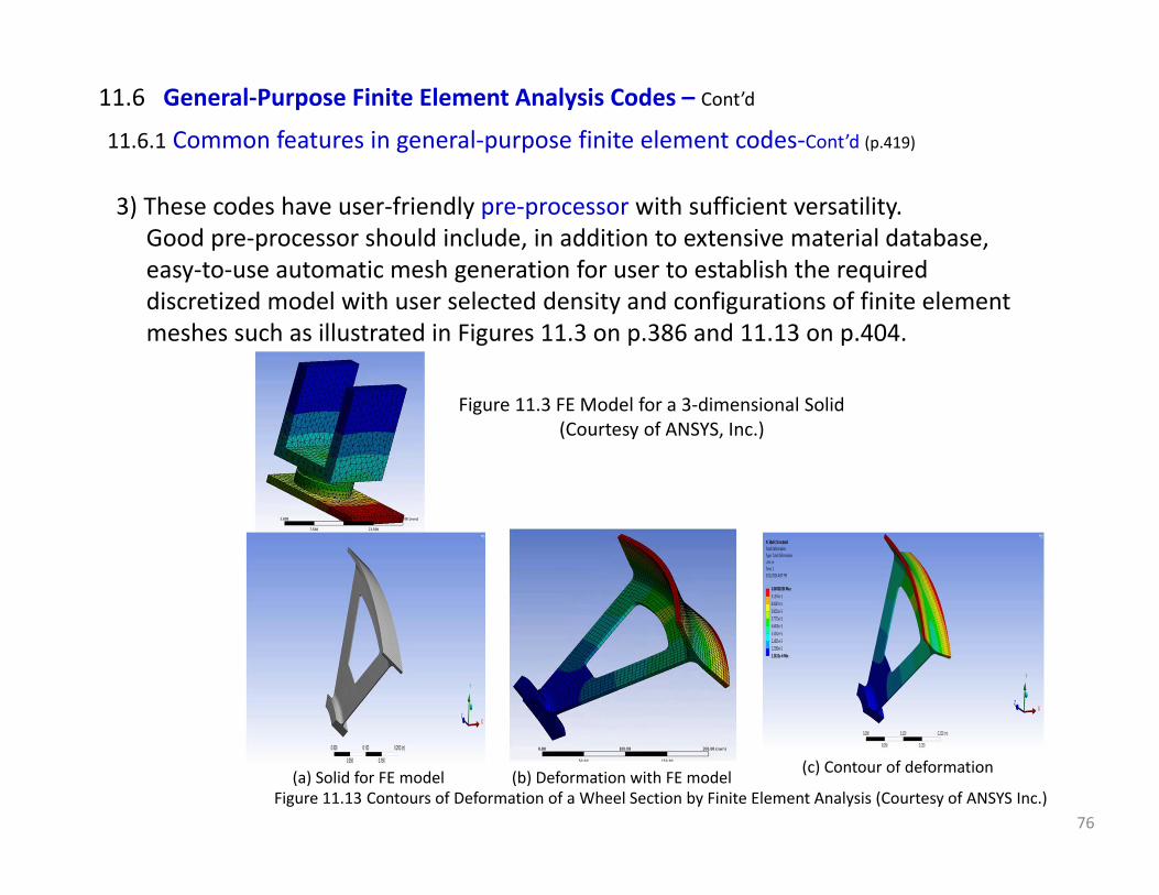
76


11.6.1 Common features in general‐purpose finite element codes‐Cont’d (p.419)

3) These codes have user‐friendly pre‐processor with sufficient versatility. Good pre‐processor should include, in addition to extensive material database, easy‐to‐use automatic mesh generation for user to establish the required discretized model with user selected density and configurations of finite element meshes such as illustrated in Figures 11.3 on p.386 and 11.13 on p.404.

Figure 11.3 FE Model for a 3‐dimensional Solid(Courtesy of ANSYS, Inc.)

(a) Solid for FE model (b) Deformation with FE model (c) Contour of deformation

Figure 11.13 Contours of Deformation of a Wheel Section by Finite Element Analysis (Courtesy of ANSYS Inc.)

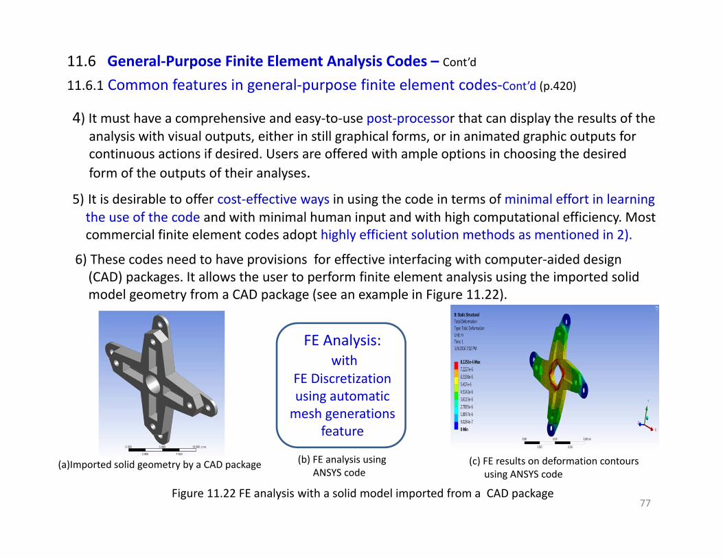
77


11.6.1 Common features in general‐purpose finite element codes‐Cont’d (p.420)

4) It must have a comprehensive and easy‐to‐use post‐processor that can display the results of the analysis with visual outputs, either in still graphical forms, or in animated graphic outputs for continuous actions if desired. Users are offered with ample options in choosing the desired form of the outputs of their analyses.

5) It is desirable to offer cost‐effective ways in using the code in terms of minimal effort in learning the use of the code and with minimal human input and with high computational efficiency. Most commercial finite element codes adopt highly efficient solution methods as mentioned in 2).

6) These codes need to have provisions for effective interfacing with computer‐aided design (CAD) packages. It allows the user to perform finite element analysis using the imported solid model geometry from a CAD package (see an example in Figure 11.22).

FE Analysis:with

FE Discretizationusing automaticmesh generations

feature

(a)Imported solid geometry by a CAD package (b) FE analysis usingANSYS code

(c) FE results on deformation contoursusing ANSYS code

Figure 11.22 FE analysis with a solid model imported from a CAD package

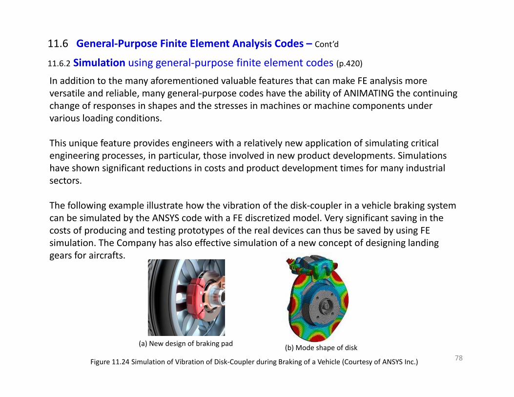
78

11.6.2 Simulation using general‐purpose finite element codes (p.420)


In addition to the many aforementioned valuable features that can make FE analysis more versatile and reliable, many general‐purpose codes have the ability of ANIMATING the continuing change of responses in shapes and the stresses in machines or machine components under various loading conditions.

This unique feature provides engineers with a relatively new application of simulating critical engineering processes, in particular, those involved in new product developments. Simulations have shown significant reductions in costs and product development times for many industrial sectors.

The following example illustrate how the vibration of the disk‐coupler in a vehicle braking system can be simulated by the ANSYS code with a FE discretized model. Very significant saving in the costs of producing and testing prototypes of the real devices can thus be saved by using FE simulation. The Company has also effective simulation of a new concept of designing landing gears for aircrafts.

(a) New design of braking pad (b) Mode shape of disk

Figure 11.24 Simulation of Vibration of Disk‐Coupler during Braking of a Vehicle (Courtesy of ANSYS Inc.)

chapter 11 finite element analysis...- slides for class teaching* chapter 11 introduction to...

Documents