chapter 12 * analysis of variance - cerritos...
TRANSCRIPT
-- 576 --
CHAPTER 12 ∇ ANALYSIS OF VARIANCE
Chapter Preview
In Chapters 8 and 9, hypothesis tests were demonstrated for testing asingle mean. Hypothesis tests between two means was subsequentlydemonstrated in Chapter 10. To continue in this fashion, Chapter 12introduces the concept of the analysis of variance technique (ANOVA)so that a hypothesis test for the equality of several means can becompleted. The F-distribution will be utilized in this test, since wewill be comparing the measures of variation (variance) among thedifferent sets of data and the measure of variation (variance) withinthe sets the data.
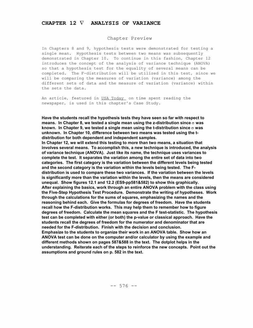
An article, featured in USA Today on time spent reading thenewspaper, is used in this chapter’s Case Study.
Have the students recall the hypothesis tests they have seen so far with respect tomeans. In Chapter 8, we tested a single mean using the z-distribution since σ wasknown. In Chapter 9, we tested a single mean using the t-distribution since σ wasunknown. In Chapter 10, difference between two means was tested using the t-distribution for both dependent and independent samples.In Chapter 12, we will extend this testing to more than two means, a situation thatinvolves several means. To accomplish this, a new technique is introduced, the analysisof variance technique (ANOVA). Just like its name, the technique uses variances tocomplete the test. It separates the variation among the entire set of data into twocategories. The first category is the variation between the different levels being testedand the second category is the variation within the levels being tested. The F-distribution is used to compare these two variances. If the variation between the levelsis significantly more than the variation within the levels, then the means are consideredunequal. Show figures 12.1 and 12.2 (ES9-pp581&582) to show this graphically.After explaining the basics, work through an entire ANOVA problem with the class usingthe Five-Step Hypothesis Test Procedure. Demonstrate the writing of hypotheses. Workthrough the calculations for the sums of squares, emphasizing the names and thereasoning behind each. Give the formulas for degrees of freedom. Have the studentsrecall how the F-distribution works. This may help them to remember how to figuredegrees of freedom. Calculate the mean squares and the F test-statistic. The hypothesistest can be completed with either (or both) the p-value or classical approach. Have thestudents recall the degrees of freedom for the numerator and denominator that areneeded for the F-distribution. Finish with the decision and conclusion.Emphasize to the students to organize their work in an ANOVA table. Show how anANOVA test can be done on the computer and/or calculator by using the example anddifferent methods shown on pages 587&588 in the text. The dotplot helps in theunderstanding. Reiterate each of the steps to reinforce the new concepts. Point out theassumptions and ground rules on p. 582 in the text.
-- 577 --
CHAPTER 12 CASE STUDY
12.1 a.
b. The mean amount of time spent reading the newspaperincreases steadily from 8.5 minutes daily for theyoungest group to 23 minutes daily for the oldest group.
SECTION 12.1 ANSWER NOW EXERCISES
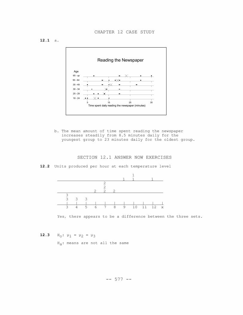
12.2 Units produced per hour at each temperature level
1 1 1 1
2 2
2 2 2 33 3 3
| | | | | | | | | | |3 4 5 6 7 8 9 10 11 12 x
Yes, there appears to be a difference between the three sets.
12.3 Ho: µ1 = µ2 = µ3
Ha: means are not all the same
5 15 25 35
Reading the Newspaper
18 - 24
25 - 29
30 - 34
35 - 49
50 - 64
65 - up
Age
Time spent daily reading the newspaper (minutes)
-- 578 --
SECTION 12.2 ANSWER NOW EXERCISES
12.4 a. Yes, there seems to be quite a bite of variation between thevalues shown on the Snapshot.
b. The male and female categories encompass the entirepopulation; as do the other 5 categories.
12.5 The 'amount of money donated' was separated into categoriesaccording to age for presentation and analyzing. ANOVA'subdivides' the data into categories of the factor, age inthis case.
SECTION 12.3 ANSWER NOW EXERCISES
12.6 a. 0 b. 2 c. 4 d. 31 e. 393
SECTION 12.3 EXERCISES
WRITING HYPOTHESES FOR THE DIFFERENCE AMONG SEVERAL MEANS
null hypothesis: Ho: µ µ µ µ1 2 3= = = =... n
or
Ho: The mean values for all n levels of the experiment are the same.[factor has no effect]
alternative hypothesis: Ha: The means are not all equal.[factor has an effect]
or
Ha: At least one mean value is different from the others.
Use subscripts on the population means that correspond to thedifferent levels or sources of the experiment.
-- 579 --
12.7 a. Ho: µ1 = µ2 = µ3 = µ4 = µ5 vs. Ha: Means not all equal[mean scores are all same]
b. Ho: µ1 = µ2 = µ3 = µ4 vs. Ha: Means not all equal[mean scores are all same]
c. Ho: µ1 = µ2 = µ3 = µ4 vs. Ha: Means not all equal[factor has no effect] [has an effect]
d. Ho: µ1 = µ2 = µ3 vs. Ha: Means not all equal[no effect] [has an effect]
Review the rules for calculating the p-value in: ES9-pp520&521, IRM-p502, if necessary. Remember to use the F-distribution, thereforeeither Tables 9a,b or c will be used to find probabilities. Review ofthe use of these tables can be found in: ES9-p517, IRM-p500.
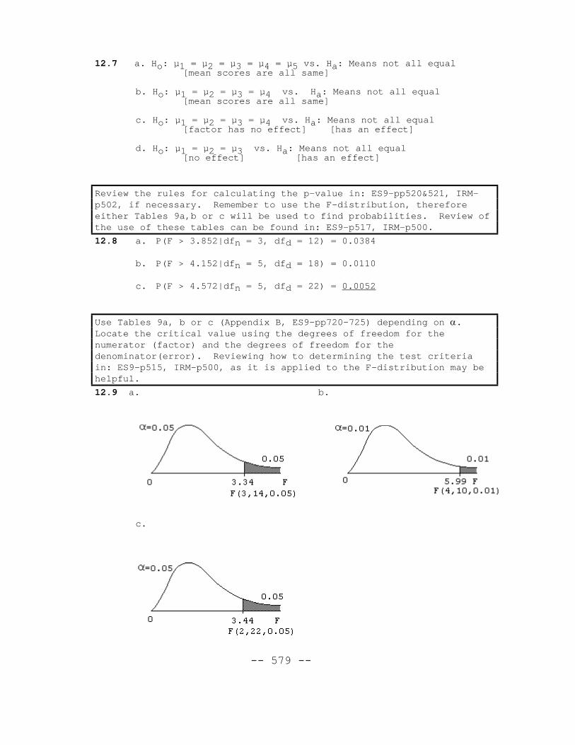
12.8 a. P(F > 3.852|dfn = 3, dfd = 12) = 0.0384
b. P(F > 4.152|dfn = 5, dfd = 18) = 0.0110
c. P(F > 4.572|dfn = 5, dfd = 22) = 0.0052
Use Tables 9a, b or c (Appendix B, ES9-pp720-725) depending on α.Locate the critical value using the degrees of freedom for thenumerator (factor) and the degrees of freedom for thedenominator(error). Reviewing how to determining the test criteriain: ES9-p515, IRM-p500, as it is applied to the F-distribution may behelpful.
12.9 a. b.
c.
-- 580 --
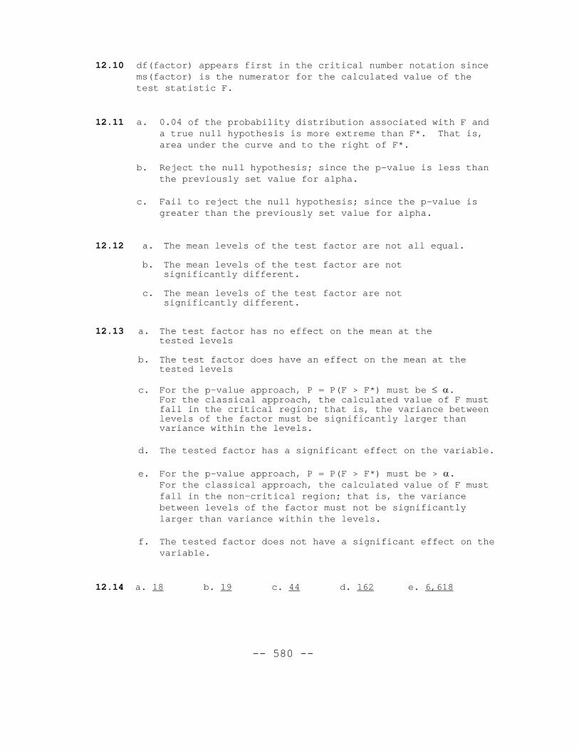
12.10 df(factor) appears first in the critical number notation sincems(factor) is the numerator for the calculated value of thetest statistic F.
12.11 a. 0.04 of the probability distribution associated with F anda true null hypothesis is more extreme than F*. That is,area under the curve and to the right of F*.
b. Reject the null hypothesis; since the p-value is less thanthe previously set value for alpha.
c. Fail to reject the null hypothesis; since the p-value isgreater than the previously set value for alpha.
12.12 a. The mean levels of the test factor are not all equal.
b. The mean levels of the test factor are notsignificantly different.
c. The mean levels of the test factor are notsignificantly different.
12.13 a. The test factor has no effect on the mean at thetested levels
b. The test factor does have an effect on the mean at thetested levels
c. For the p-value approach, P = P(F > F*) must be ≤ α. For the classical approach, the calculated value of F mustfall in the critical region; that is, the variance betweenlevels of the factor must be significantly larger thanvariance within the levels.
d. The tested factor has a significant effect on the variable.
e. For the p-value approach, P = P(F > F*) must be > α. For the classical approach, the calculated value of F mustfall in the non-critical region; that is, the variancebetween levels of the factor must not be significantlylarger than variance within the levels.
f. The tested factor does not have a significant effect on thevariable.
12.14 a. 18 b. 19 c. 44 d. 162 e. 6,618
-- 581 --
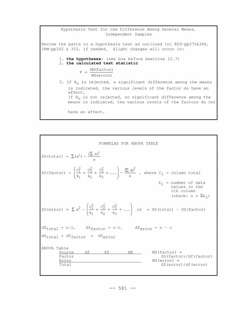
Hypothesis Test for the Difference Among Several Means,Independent Samples
Review the parts to a hypothesis test as outlined in: ES9-pp370&386,IRM-pp342 & 353, if needed. Slight changes will occur in:
1. the hypotheses: (see box before exercise 12.7)2. the calculated test statistic
FMS factor
MS error=
( )
( )
3. If Ho is rejected, a significant difference among the means
is indicated, the various levels of the factor do have aneffect.If Ho is not rejected, no significant difference among the means is indicated, the various levels of the factors do not
have an effect.
FORMULAS FOR ANOVA TABLE
SS(total) = ∑ −∑
( )( )
xx
n2
2
SS(factor) = n
)x(...
k
C
k
C
k
C 2
3
23
2
22
1
21 ∑
−
+++ , where Ci = column total
ki = number of data values in the ith column
(check: n = Σki)
SS(error) =
+++−∑ ...
k
C
k
C
k
Cx
3
23
2
22
1
212 or = SS(total) - SS(factor)
dftotal = n-1, dffactor = c-1, dferror = n - c
dftotal = dffactor + dferror
ANOVA TableSource df SS MS MS(factor) = Factor SS(factor)/df(factor)Error MS(error) =Total SS(error)/df(error)
-- 582 --
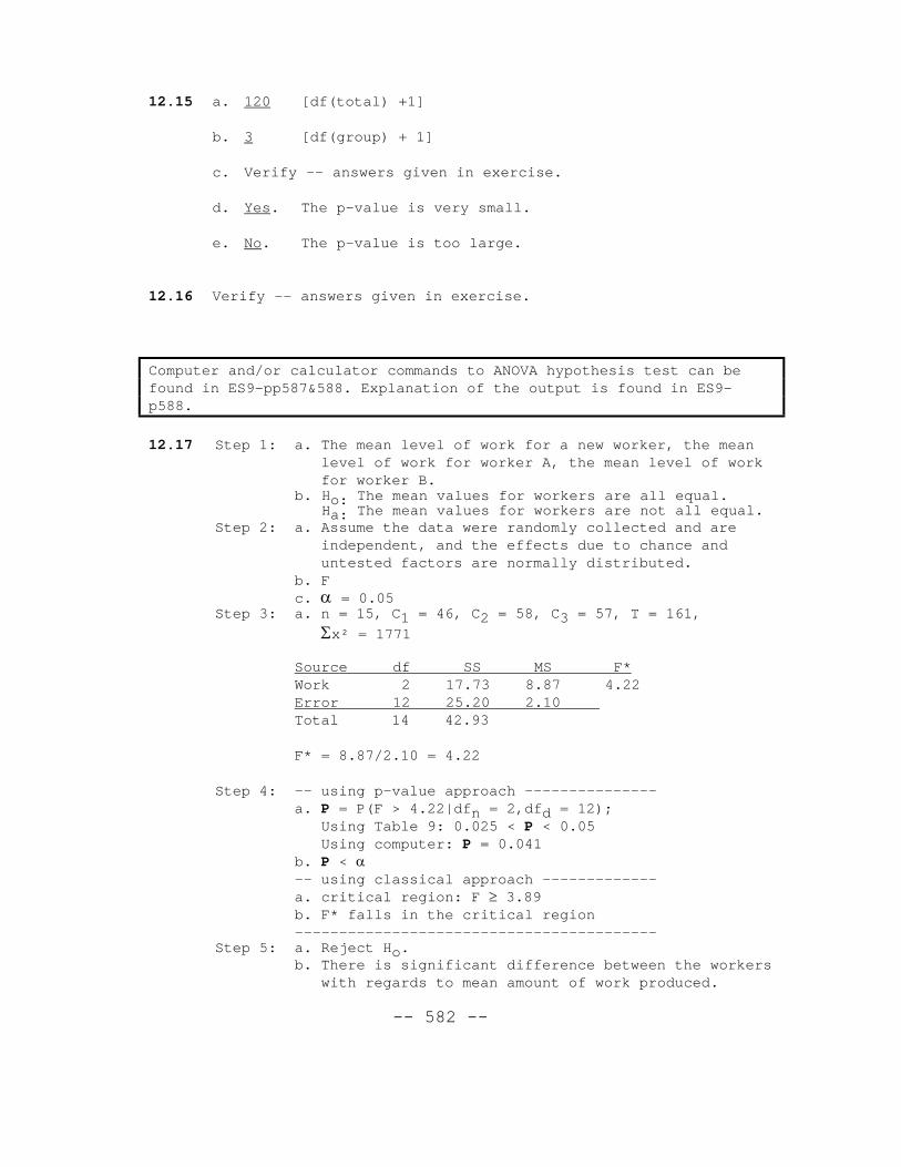
12.15 a. 120 [df(total) +1]
b. 3 [df(group) + 1]
c. Verify -- answers given in exercise.
d. Yes. The p-value is very small.
e. No. The p-value is too large.
12.16 Verify -- answers given in exercise.
Computer and/or calculator commands to ANOVA hypothesis test can befound in ES9-pp587&588. Explanation of the output is found in ES9-p588.
12.17 Step 1: a. The mean level of work for a new worker, the meanlevel of work for worker A, the mean level of workfor worker B.
b. Ho: The mean values for workers are all equal.Ha: The mean values for workers are not all equal.
Step 2: a. Assume the data were randomly collected and areindependent, and the effects due to chance anduntested factors are normally distributed.
b. Fc. α = 0.05
Step 3: a. n = 15, C1 = 46, C2 = 58, C3 = 57, T = 161,
Σx² = 1771
Source df SS MS F*Work 2 17.73 8.87 4.22Error 12 25.20 2.10 Total 14 42.93
F* = 8.87/2.10 = 4.22
Step 4: -- using p-value approach ---------------a. P = P(F > 4.22|dfn = 2,dfd = 12);
Using Table 9: 0.025 < P < 0.05 Using computer: P = 0.041
b. P < α-- using classical approach -------------a. critical region: F ≥ 3.89b. F* falls in the critical region-----------------------------------------
Step 5: a. Reject Ho.b. There is significant difference between the workers
with regards to mean amount of work produced.
-- 583 --
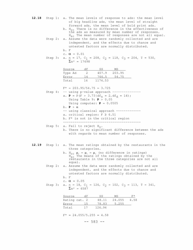
12.18 Step 1: a. The mean levels of response to ads: the mean levelof big headline ads, the mean level of straightforward ads, the mean level of bold print ads.
b. Ho: There is no difference in the effectiveness ofthe ads as measured by mean number of responses.Ha: The mean number of responses are not all equal.
Step 2: a. Assume the data were randomly collected and areindependent, and the effects due to chance anduntested factors are normally distributed.
b. Fc. α = 0.01
Step 3: a. n = 17, C1 = 208, C2 = 118, C3 = 204, T = 530, Σx² = 17698
Source df SS MS Type Ad 2 407.9 203.95Error 14 766.5 54.75 Total 16 1174.53
F* = 203.95/54.75 = 3.725Step 4: -- using p-value approach ---------------
a. P = P(F > 3.73|dfn = 2,dfd = 14);Using Table 9: P > 0.05 Using computer: P = 0.0505
b. P > α-- using classical approach -------------a. critical region: F ≥ 6.51b. F* is not in the critical region-----------------------------------------
Step 5: a. Fail to reject Ho.b. There is no significant difference between the ads
with regards to mean number of responses.
12.19 Step 1: a. The mean ratings obtained by the restaurants in thethree categories.
b. Ho: µF = µD = µS (no difference in ratings)Ha: The means of the ratings obtained by therestaurants in the three categories are not allequal.
Step 2: a. Assume the data were randomly collected and areindependent, and the effects due to chance anduntested factors are normally distributed.
b. Fc. α = 0.05
Step 3: a. n = 18, C1 = 126, C2 = 102, C3 = 113, T = 341, Σx² = 6587
Source df SS MS F*Rating cat. 2 48.11 24.055 4.58Error 15 78.83 5.255 Total 17 126.94
F* = 24.055/5.255 = 4.58
-- 584 --
Step 4: -- using p-value approach ---------------a. P = P(F > 4.58|dfn = 2,dfd = 15);
Using Table 9: 0.025 P < 0.05 Using computer: P = 0.028
b. P < α-- using classical approach -------------a. critical region: F ≥ 3.68b. F* is in the critical region-----------------------------------------
Step 5: a. Reject Ho.b. The data shows significant evidence that would give
reason to reject the null hypothesis that the meansof the three categories of ratings given to therestaurants are not equal.
12.20 a. Step 1: a. The mean oat-production yield rates for six states.b. Ho: The mean yield rate is the same for each of the
six states.Ha: The mean yield rate is not the same for each of
the six states.Step 2: a. Assume the data were randomly collected and are
independent, and the effects due to chance anduntested factors are normally distributed.
b. Fc. α = 0.05
Step 3: a. n = 39, C1 = 612.40, C2 = 352, C3 = 329.80, C4 = 314, C5 = 405.10, C6 = 379, T = 2392.3, Σx² = 151151
Source df SS MS F* Factor 5 1145.1 229.0 2.32Error 33 3259.9 98.8Total 38 4405.0
Step 4: -- using p-value approach ---------------a. P = P(F > 2.32|dfn = 5,dfd = 33);
Using Table 9: P > 0.05Using computer: P = 0.065
b. P > α-- using classical approach -------------a. F(5,33,0.05) = 2.53b. F* is not in the critical region-----------------------------------------
Step 5: a. Fail to reject Ho.b. There is not sufficient evidence to show that at
least one mean is significantly different from theothers at the 0.05 level of significance.
-- 585 --
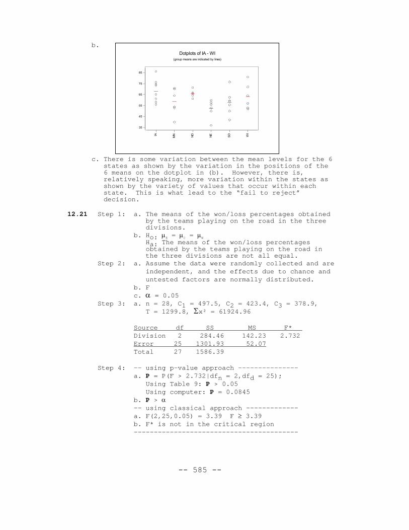
b.
c. There is some variation between the mean levels for the 6states as shown by the variation in the positions of the6 means on the dotplot in (b). However, there is,relatively speaking, more variation within the states asshown by the variety of values that occur within eachstate. This is what lead to the “fail to reject”decision.
12.21 Step 1: a. The means of the won/loss percentages obtainedby the teams playing on the road in the threedivisions.
b. Ho: µE = µC = µW
Ha: The means of the won/loss percentagesobtained by the teams playing on the road inthe three divisions are not all equal.
Step 2: a. Assume the data were randomly collected and areindependent, and the effects due to chance anduntested factors are normally distributed.
b. Fc. α = 0.05
Step 3: a. n = 28, C1 = 497.5, C2 = 423.4, C3 = 378.9, T = 1299.8, Σx² = 61924.96
Source df SS MS F* Division 2 284.46 142.23 2.732Error 25 1301.93 52.07Total 27 1586.39
Step 4: -- using p-value approach ---------------a. P = P(F > 2.732|dfn = 2,dfd = 25);
Using Table 9: P > 0.05Using computer: P = 0.0845
b. P > α-- using classical approach -------------a. F(2,25,0.05) = 3.39 F ≥ 3.39b. F* is not in the critical region-----------------------------------------
IA
MN
ND
NE
SD WI
35
45
55
65
75
85
Dotplots of IA - WI(group means are indicated by lines)
-- 586 --
Step 5: a. Fail to reject Ho.b. The data shows no significant evidence that would
give reason to reject the null hypothesis that themeans of the won/loss percentages obtained by theteams playing on the road in the three divisionsare equal.
12.22 Step 1: a. The mean age of three test groups: the mean age forthe TTS group, the mean age for the Antivert group,the mean age for the placebo group.
b. Ho: The mean age for groups are all equal.Ha: The mean age for groups are not all equal.
Step 2: a. Assume the data were randomly collected and areindependent, and the effects due to chance anduntested factors are normally distributed.
b. Fc. α = 0.05
Step 3: a. n = 58, k1 = 18, C1 = 846, k2 = 21, C2 = 894, k3 = 19, C3 = 805, T = 2545, Σx² = 120,549
Source df SS MS F* Group 2 254.591 127.30 0.81Error 55 8621.564 156.76 Total 57 8876.155
Step 4: -- using p-value approach ---------------a. P = P(F > 0.81|dfn = 2,dfd = 55);
Using Table 9: P > 0.05Using computer: P = 0.449
b. P > α-- using classical approach -------------a. F(2,55,0.05) ≈ 3.15 F ≥ 3.15b. F* is not in the critical region-----------------------------------------
Step 5: a. Fail to reject Ho.b. The data does not show a significant difference
between the mean ages of the groups.
12.23 Calories:Step 1: a. The means of the calories contained in the four
snack categories are not all equal.b. Ho: µ1 = µ2 = µ3 = µ4
Ha: The means of the calories contained in the foursnack categories are not all equal.
Step 2: a. Assume the data were randomly collected and areindependent, and the effects due to chance anduntested factors are normally distributed.
b. Fc. α = 0.01
-- 587 --
Step 3: a. n = 50, k1 = 12, C1 = 1029, k2 = 10, C2 = 557, k3 = 12, C3 = 1033, k4 = 16, C4 = 1342, T = 3961, Σx² = 338265
Source df SS MS F* Category 3 6955.56 2318.52 6.088Error 46 17519.02 380.85Total 49 24474.58
Step 4: -- using p-value approach ---------------a. P = P(F > 6.088|dfn = 3,dfd = 46);
Using Table 9: P < 0.01Using computer: P = 0.0014
b. P < α-- using classical approach -------------a. F(3,46,0.01) ≈ 4.26 F ≥ 4.26b. F* is in the critical region-----------------------------------------
Step 5: a. Reject Ho.b. The data shows significant evidence that would give
reason to reject the null hypothesis that thecalories contained by the snacks in each categoryare not equal.
Fat content:Step 1: a. The mean age of three test groups: the mean age for
the TTS group, the mean age for the Antivert group,the mean age for the placebo group.
b. Ho: µ1 = µ2 = µ3 = µ4
Ha: The means of the grams of fat contained in thefour snack categories are not all equal.
Step 2: a. Assume the data were randomly collected and areindependent, and the effects due to chance anduntested factors are normally distributed.
b. Fc. α = 0.01
Step 3: a. n = 50, k1 = 12, C1 = 25.3, k2 = 10, C2 = 12.4, k3 = 12, C3 = 28.2, k4 = 16, C4 = 12.1, T = 78.0, Σx² = 341.4
Source df SS MS F* Category 3 22.46 7.49 1.745Error 46 197.26 4.29Total 49 219.72
Step 4: -- using p-value approach ---------------a. P = P(F > 1.745|dfn = 3,dfd = 46);
Using Table 9: P > 0.05Using computer: P = 0.171
b. P > α-- using classical approach -------------a. F(3,46,0.01) ≈ 4.26 F ≥ 4.26b. F* is not in the critical region-----------------------------------------
-- 588 --
Step 5: a. Fail to reject Ho.b. The data shows no significant evidence that
would give reason to reject the nullhypothesis that the grams of fat contained bythe snacks in each category are not equal.
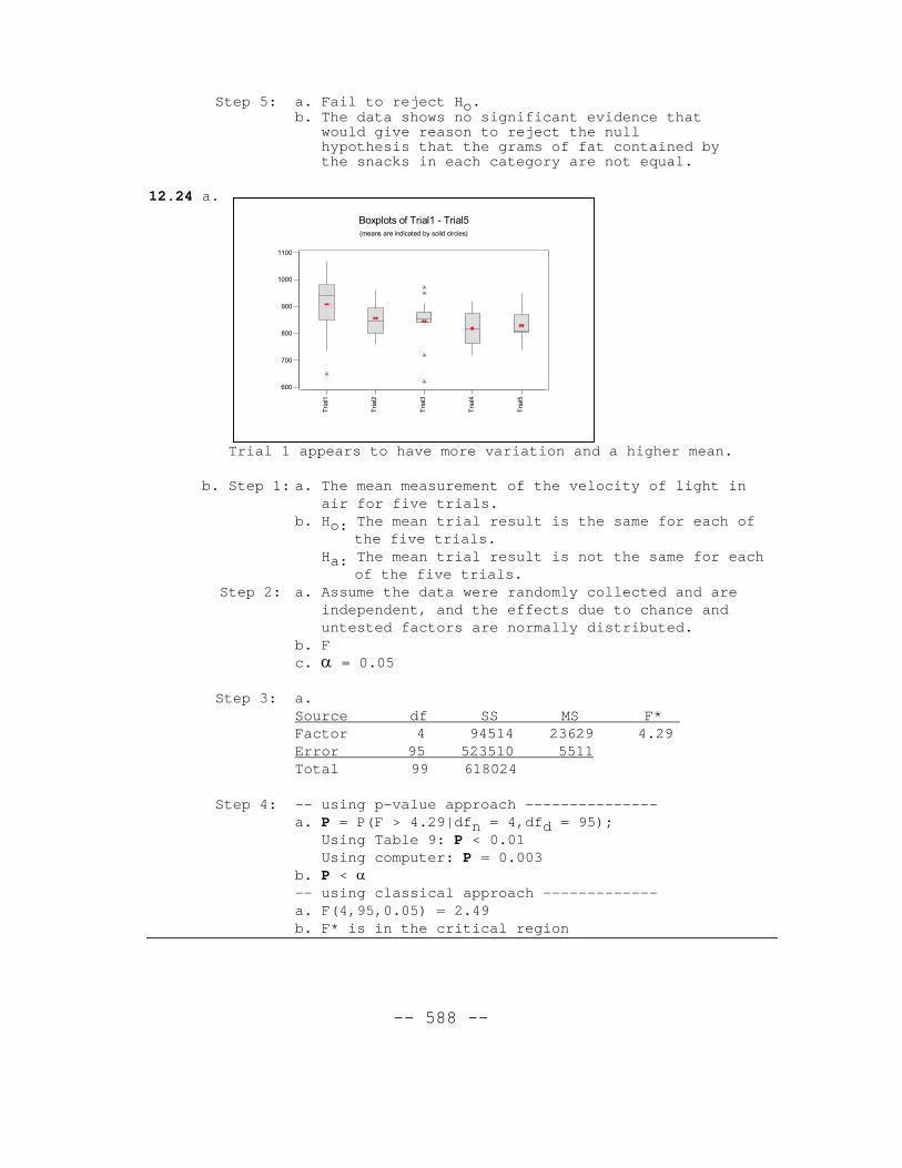
12.24 a.
Trial 1 appears to have more variation and a higher mean.
b. Step 1: a. The mean measurement of the velocity of light inair for five trials.
b. Ho: The mean trial result is the same for each ofthe five trials.
Ha: The mean trial result is not the same for eachof the five trials.
Step 2: a. Assume the data were randomly collected and areindependent, and the effects due to chance anduntested factors are normally distributed.
b. Fc. α = 0.05
Step 3: a. Source df SS MS F* Factor 4 94514 23629 4.29Error 95 523510 5511Total 99 618024
Step 4: -- using p-value approach ---------------a. P = P(F > 4.29|dfn = 4,dfd = 95);
Using Table 9: P < 0.01Using computer: P = 0.003
b. P < α-- using classical approach -------------a. F(4,95,0.05) = 2.49b. F* is in the critical region
Tria
l1
Tria
l2
Tria
l3
Tria
l4
Tria
l5
600
700
800
900
1000
1100
Boxplots of Trial1 - Trial5(means are indicated by solid circles)
-- 589 --
Step 5: a. Reject Ho.b. There is sufficient evidence to show that at least
one mean is significantly different from the othersat the 0.05 level of significance.
c. The first trial had the highest mean and largest standarddeviation. These results may have been due to start upprocedures and methods.
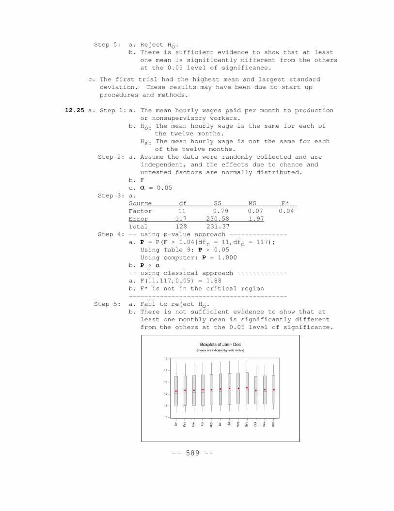
12.25 a. Step 1: a. The mean hourly wages paid per month to productionor nonsupervisory workers.
b. Ho: The mean hourly wage is the same for each ofthe twelve months.
Ha: The mean hourly wage is not the same for eachof the twelve months.
Step 2: a. Assume the data were randomly collected and areindependent, and the effects due to chance anduntested factors are normally distributed.
b. Fc. α = 0.05
Step 3: a. Source df SS MS F* Factor 11 0.79 0.07 0.04Error 117 230.58 1.97Total 128 231.37
Step 4: -- using p-value approach ---------------a. P = P(F > 0.04|dfn = 11,dfd = 117);
Using Table 9: P > 0.05Using computer: P = 1.000
b. P > α-- using classical approach -------------a. F(11,117,0.05) = 1.88b. F* is not in the critical region-----------------------------------------
Step 5: a. Fail to reject Ho.b. There is not sufficient evidence to show that at
least one monthly mean is significantly differentfrom the others at the 0.05 level of significance.
Jan
Fe
b
Mar
Ap
r
May Ju
n
Jul
Aug
Se
p
Oct
No
v
De
c
10
11
12
13
14
15
Boxplots of Jan - Dec(means are indicated by solid circles)
-- 590 --
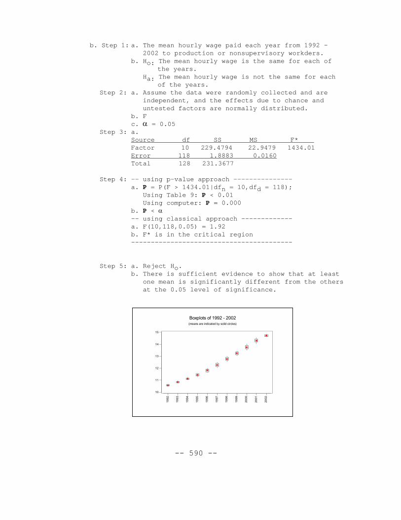
b. Step 1: a. The mean hourly wage paid each year from 1992 –2002 to production or nonsupervisory workders.
b. Ho: The mean hourly wage is the same for each ofthe years.
Ha: The mean hourly wage is not the same for eachof the years.
Step 2: a. Assume the data were randomly collected and areindependent, and the effects due to chance anduntested factors are normally distributed.
b. Fc. α = 0.05
Step 3: a. Source df SS MS F* Factor 10 229.4794 22.9479 1434.01Error 118 1.8883 0.0160Total 128 231.3677
Step 4: -- using p-value approach ---------------a. P = P(F > 1434.01|dfn = 10,dfd = 118);
Using Table 9: P < 0.01Using computer: P = 0.000
b. P < α-- using classical approach -------------a. F(10,118,0.05) = 1.92b. F* is in the critical region-----------------------------------------
Step 5: a. Reject Ho.b. There is sufficient evidence to show that at least
one mean is significantly different from the othersat the 0.05 level of significance.
19
92
19
93
19
94
19
95
19
96
19
97
19
98
19
99
20
00
20
01
20
02
10
11
12
13
14
15
Boxplots of 1992 - 2002(means are indicated by solid circles)
-- 591 --
RETURN TO CHAPTER CASE STUDY
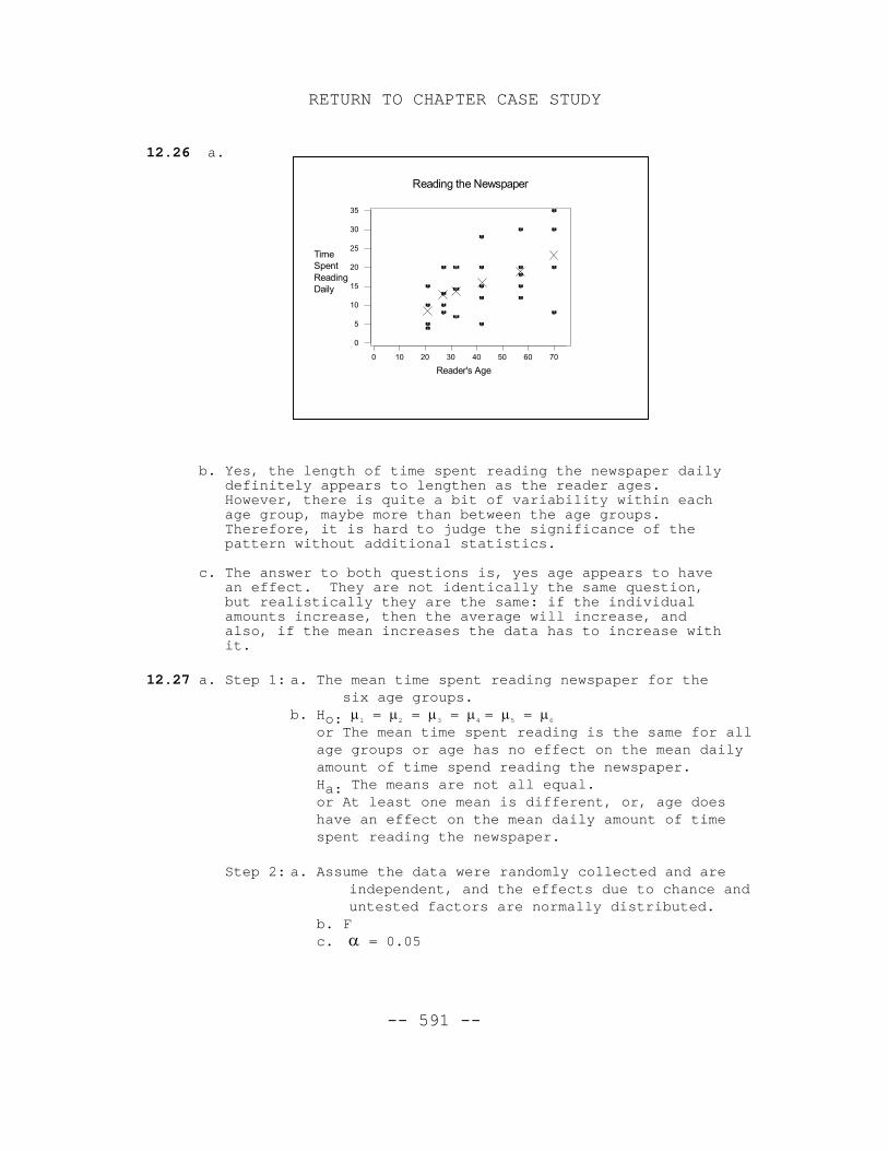
12.26 a.
b. Yes, the length of time spent reading the newspaper dailydefinitely appears to lengthen as the reader ages.However, there is quite a bit of variability within eachage group, maybe more than between the age groups.Therefore, it is hard to judge the significance of thepattern without additional statistics.
c. The answer to both questions is, yes age appears to havean effect. They are not identically the same question,but realistically they are the same: if the individualamounts increase, then the average will increase, andalso, if the mean increases the data has to increase withit.
12.27 a. Step 1: a. The mean time spent reading newspaper for thesix age groups.
b. Ho: µ1 = µ2 = µ3 = µ4 = µ5 = µ6
or The mean time spent reading is the same for allage groups or age has no effect on the mean dailyamount of time spend reading the newspaper.
Ha: The means are not all equal.or At least one mean is different, or, age doeshave an effect on the mean daily amount of timespent reading the newspaper.
Step 2: a. Assume the data were randomly collected and areindependent, and the effects due to chance anduntested factors are normally distributed.
b. Fc. α = 0.05
0 10 20 30 40 50 60 70
0
5
10
15
20
25
30
35
Reader's Age
TimeSpentReadingDaily
Reading the Newspaper
-- 592 --
Step 3: a. n = 25, k1 = 4, C1 = 34, k2 = 4, C2 = 51, k3 = 3, C3 = 41, k4 = 5, C4 = 80, k5 = 5,
C5 = 95, k6 = 4, C6 = 93, T = 394, Σx² = 7904
Source df SS MS F* Age 5 537.4 107.5 1.76Error 19 1157.2 60.9Total 24 1694.6
Step 4: -- using p-value approach ---------------a. P = P(F > 1.76|dfn = 5,dfd = 19); Using Table 9: P > 0.05 Using computer: P = 0.168b. P > α-- using classical approach -------------a. F(5,19,0.05) = 2.74b. F* is not in the critical region-----------------------------------------
Step 5: a. Fail to reject Ho.b. The data does not show significant evidence
to conclude the mean amount of time spentreading newspaper yesterday is effected byage, at the 0.05 level of significance.
b. The amount of variability within the age groups is toolarge, relatively speaking, for the amount of variabilitybetween age groups to be significant.
12.28 Answers will vary.
CHAPTER EXERCISES
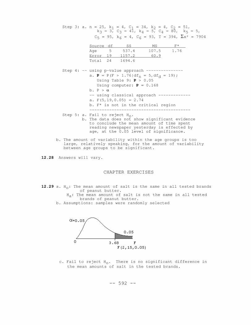
12.29 a. Ho: The mean amount of salt is the same in all tested brandsof peanut butter.
Ha: The mean amount of salt is not the same in all testedbrands of peanut butter.
b. Assumptions: samples were randomly selected
c. Fail to reject Ho. There is no significant difference inthe mean amounts of salt in the tested brands.
-- 593 --
d. Since the p-value is quite large (much larger than 0.05), ittells us the sample data is quite likely to have occurredunder the assumed conditions and a true null hypothesis.Therefore, we 'fail to reject Ho.'
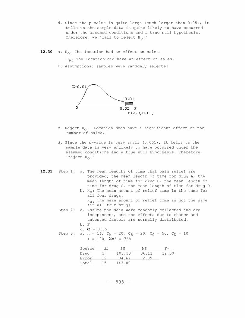
12.30 a. Ho: The location had no effect on sales.
Ha: The location did have an effect on sales.
b. Assumptions: samples were randomly selected
c. Reject Ho. Location does have a significant effect on thenumber of sales.
d. Since the p-value is very small (0.001), it tells us thesample data is very unlikely to have occurred under theassumed conditions and a true null hypothesis. Therefore, 'reject Ho.'
12.31 Step 1: a. The mean lengths of time that pain relief areprovided; the mean length of time for drug A, themean length of time for drug B, the mean length oftime for drug C, the mean length of time for drug D.
b. Ho: The mean amount of relief time is the same forall four drugs.Ha: The mean amount of relief time is not the samefor all four drugs.
Step 2: a. Assume the data were randomly collected and areindependent, and the effects due to chance anduntested factors are normally distributed.
b. Fc. α = 0.05
Step 3: a. n = 16, CA = 20, CB = 20, CC = 50, CD = 10,
T = 100, Σx² = 768
Source df SS MS F* Drug 3 108.33 36.11 12.50Error 12 34.67 2.89 Total 15 143.00
-- 594 --
Step 4: -- using p-value approach ---------------a. P = P(F > 12.50|dfn = 3,dfd = 12);
Using Table 9: P < 0.01Using computer: P = 0.001
b. P < α-- using classical approach -------------a. critical value: F(3,12,0.05) = 3.49
critical region: F ≥ 3.49b. F* is in the critical region
-----------------------------------------Step 5: b. Reject Ho.
c. There is a significant difference between the mean amount of time one gets relief from these four drugs.
12.32 Step 1: a. The mean stopping distance on wet pavement for eachbrand of tire.
b. Ho: The mean stopping distance is not affected bythe brand of tire.Ha: The mean stopping distance is affected by therand of tire.
Step 2: a. Assume the data were randomly collected and areindependent, and the effects due to chance anduntested factors are normally distributed.
b. Fc. α = 0.05
Step 3: a. n = 23, CA = 217, CB = 194, CC = 216, CD = 245 T = 872, Σx² = 33,282Source df SS MS F* Brand 3 95.36 31.79 4.78Error 19 126.47 6.66 Total 22 221.83
Step 4: -- using p-value approach ---------------a. P = P(F > 4.78|dfn = 3,dfd = 19);
Using Table 9: 0.01 < P < 0.025Using computer: P = 0.012
b. P < α-- using classical approach -------------a. critical value: F(3,19,0.05) = 3.13
critical region: F ≥ 3.13b. F* is in the critical region-----------------------------------------
Step 5: b. Reject Ho.c. There is a significant difference between the mean stopping distance for the different tire brands.
-- 595 --
12.33 Step 1: a. The mean amounts of soft drink dispensed: the meanamount for machine A, the mean amount for machineB, the mean amount for machine C, the mean amountfor machine D, the mean amount for machine E.
b. Ho: The mean amounts dispensed by the machines areall equal.Ha: The mean amounts dispensed by the machines arenot all equal.
Step 2: a. Assume the data were randomly collected and areindependent, and the effects due to chance anduntested factors are normally distributed.
b. Fc. α = 0.01
Step 3: a. n = 18, CA = 16.5, CB = 20.6, CC = 16.9, CD = 19.1, CE = 21.8, T = 94.9, Σx² = 523.49
Source df SS MS F* Machine 4 20.998 5.2495 31.6Error 13 2.158 0.166 Total 17 23.156
Step 4: -- using p-value approach ---------------a. P = P(F > 31.6|dfn = 4,dfd = 13);
Using Table 9: P < 0.01Using computer: P = 0.000
b. P < α-- using classical approach -------------a. critical value: F(4,13,0.01) = 5.21
critical region: F ≥ 5.21b. F* is in the critical region
-----------------------------------------Step 5: a. Reject Ho.
b. There is a significant difference between the machines with regards to mean amount of soft drink dispensed.
12.34 a.Step 1: a. The mean transfer values for five suburbs: the mean
transfer value for suburb A, the mean transfervalue for suburb B, the mean transfer value forsuburb C, the mean transfer value for suburb D, themean transfer value for suburb E.
b. Ho: The mean transfer value is the same for allfive suburbs.Ha: The mean transfer value is not the same for allfive suburbs.
Step 2: a. Assume the data were randomly collected and areindependent, and the effects due to chance anduntested factors are normally distributed.
b. Fc. α = 0.01
-- 596 --
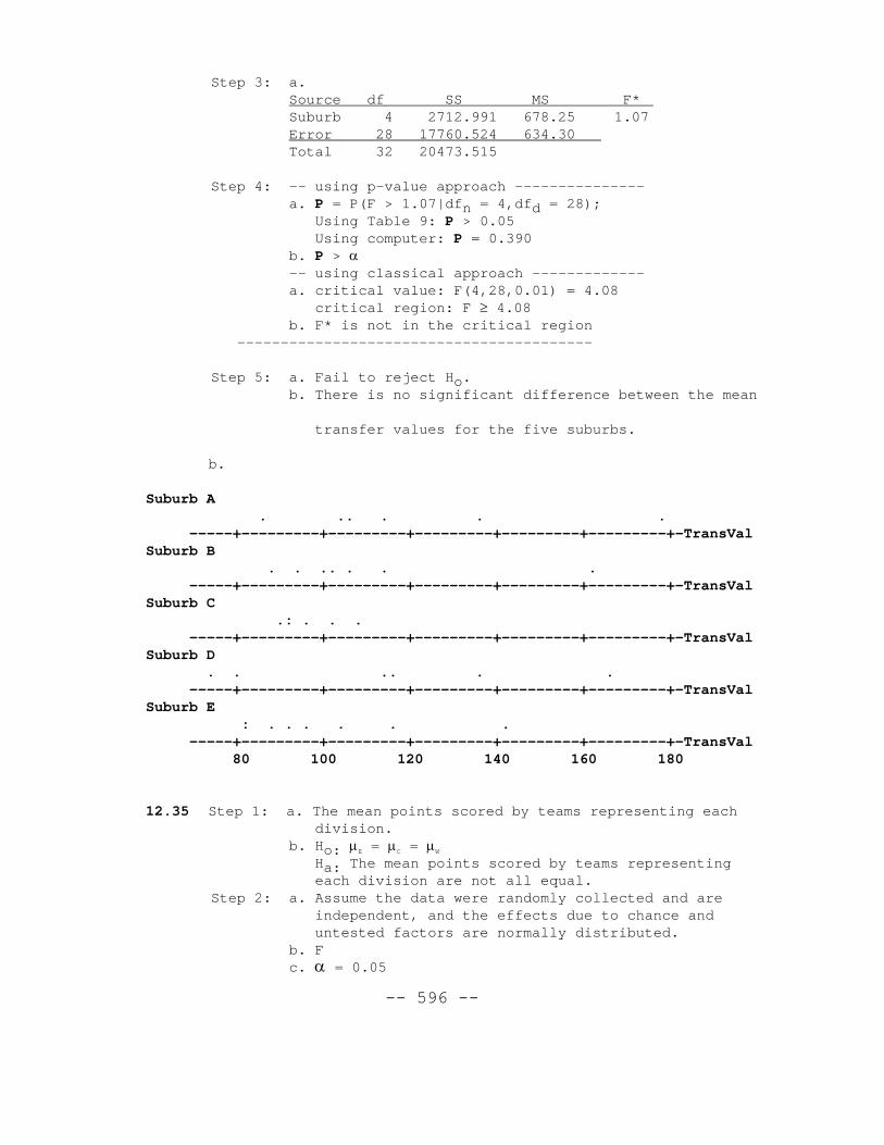
Step 3: a. Source df SS MS F* Suburb 4 2712.991 678.25 1.07Error 28 17760.524 634.30 Total 32 20473.515
Step 4: -- using p-value approach ---------------a. P = P(F > 1.07|dfn = 4,dfd = 28);
Using Table 9: P > 0.05Using computer: P = 0.390
b. P > α-- using classical approach -------------a. critical value: F(4,28,0.01) = 4.08
critical region: F ≥ 4.08b. F* is not in the critical region
-----------------------------------------
Step 5: a. Fail to reject Ho.b. There is no significant difference between the mean
transfer values for the five suburbs.
b.
Suburb A . .. . . . -----+---------+---------+---------+---------+---------+-TransValSuburb B . . .. . . . -----+---------+---------+---------+---------+---------+-TransValSuburb C .: . . . -----+---------+---------+---------+---------+---------+-TransValSuburb D . . .. . . -----+---------+---------+---------+---------+---------+-TransValSuburb E : . . . . . . -----+---------+---------+---------+---------+---------+-TransVal 80 100 120 140 160 180
12.35 Step 1: a. The mean points scored by teams representing eachdivision.
b. Ho: µE = µC = µW
Ha: The mean points scored by teams representingeach division are not all equal.
Step 2: a. Assume the data were randomly collected and areindependent, and the effects due to chance anduntested factors are normally distributed.
b. Fc. α = 0.05
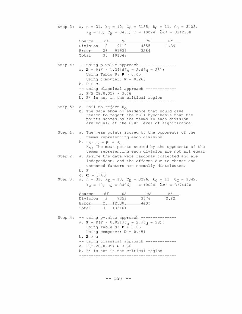
-- 597 --
Step 3: a. n = 31, kE = 10, CE = 3135, kC = 11, CC = 3408,
kW = 10, CW = 3481, T = 10024, Σx² = 3342358
Source df SS MS F* Division 2 9110 4555 1.39Error 28 91939 3284Total 30 101049
Step 4: -- using p-value approach ---------------a. P = P(F > 1.39|dfn = 2,dfd = 28);
Using Table 9: P > 0.05Using computer: P = 0.266
b. P > α-- using classical approach -------------a. F(2,28,0.05) ≈ 3.36b. F* is not in the critical region-----------------------------------------
Step 5: a. Fail to reject Ho.b. The data show no evidence that would give
reason to reject the null hypothesis that thepoints scored by the teams in each divisionare equal, at the 0.05 level of significance.
Step 1: a. The mean points scored by the opponents of theteams representing each division.
b. Ho: µE = µC = µW
Ha: The mean points scored by the opponents of theteams representing each division are not all equal.
Step 2: a. Assume the data were randomly collected and areindependent, and the effects due to chance anduntested factors are normally distributed.
b. Fc. α = 0.05
Step 3: a. n = 31, kE = 10, CE = 3276, kC = 11, CC = 3342,
kW = 10, CW = 3406, T = 10024, Σx² = 3374470
Source df SS MS F* Division 2 7353 3676 0.82Error 28 125808 4493Total 30 133161
Step 4: -- using p-value approach ---------------a. P = P(F > 0.82|dfn = 2,dfd = 28);
Using Table 9: P > 0.05Using computer: P = 0.451
b. P > α-- using classical approach -------------a. F(2,28,0.05) ≈ 3.36b. F* is not in the critical region-----------------------------------------
-- 598 --
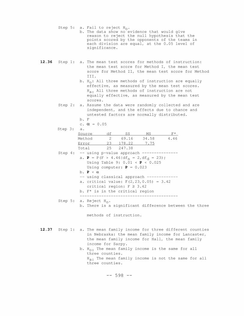
Step 5: a. Fail to reject Ho.b. The data show no evidence that would give
reason to reject the null hypothesis that thepoints scored by the opponents of the teams ineach division are equal, at the 0.05 level ofsignificance.
12.36 Step 1: a. The mean test scores for methods of instruction:the mean test score for Method I, the mean testscore for Method II, the mean test score for MethodIII.
b. Ho: All three methods of instruction are equally effective, as measured by the mean test scores.Ha: All three methods of instruction are notequally effective, as measured by the mean testscores.
Step 2: a. Assume the data were randomly collected and areindependent, and the effects due to chance anduntested factors are normally distributed.
b. Fc. α = 0.05
Step 3: a.Source df SS MS F* Method 2 69.16 34.58 4.46Error 23 178.22 7.75Total 25 247.38
Step 4: -- using p-value approach ---------------a. P = P(F > 4.46|dfn = 2,dfd = 23);
Using Table 9: 0.01 < P < 0.025Using computer: P = 0.023
b. P < α-- using classical approach -------------a. critical value: F(2,23,0.05) = 3.42
critical region: F ≥ 3.42b. F* is in the critical region-----------------------------------------
Step 5: a. Reject Ho.b. There is a significant difference between the three
methods of instruction.
12.37 Step 1: a. The mean family income for three different countiesin Nebraska: the mean family income for Lancaster,the mean family income for Hall, the mean familyincome for Sarpy.
b. Ho: The mean family income is the same for allthree counties.Ha: The mean family income is not the same for allthree counties.
-- 599 --
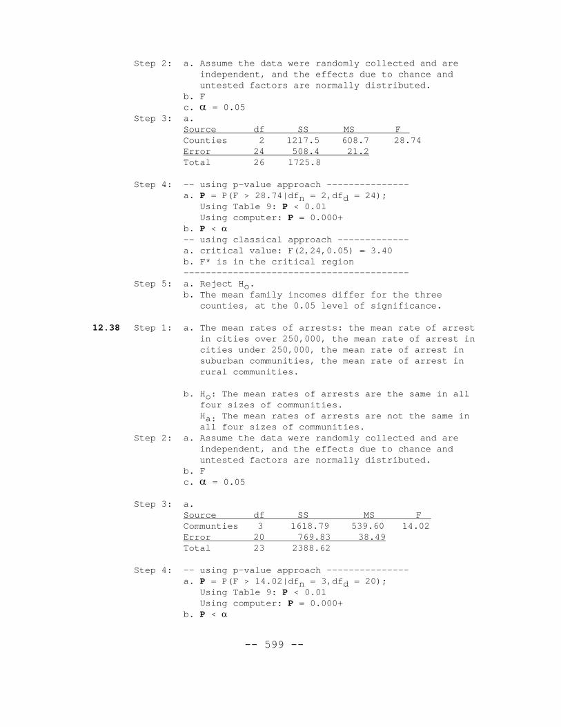
Step 2: a. Assume the data were randomly collected and areindependent, and the effects due to chance anduntested factors are normally distributed.
b. Fc. α = 0.05
Step 3: a. Source df SS MS F Counties 2 1217.5 608.7 28.74Error 24 508.4 21.2Total 26 1725.8
Step 4: -- using p-value approach ---------------a. P = P(F > 28.74|dfn = 2,dfd = 24);
Using Table 9: P < 0.01Using computer: P = 0.000+
b. P < α-- using classical approach -------------a. critical value: F(2,24,0.05) = 3.40b. F* is in the critical region-----------------------------------------
Step 5: a. Reject Ho.b. The mean family incomes differ for the three
counties, at the 0.05 level of significance.
12.38 Step 1: a. The mean rates of arrests: the mean rate of arrestin cities over 250,000, the mean rate of arrest incities under 250,000, the mean rate of arrest insuburban communities, the mean rate of arrest inrural communities.
b. Ho: The mean rates of arrests are the same in allfour sizes of communities.Ha: The mean rates of arrests are not the same inall four sizes of communities.
Step 2: a. Assume the data were randomly collected and areindependent, and the effects due to chance anduntested factors are normally distributed.
b. Fc. α = 0.05
Step 3: a. Source df SS MS F Communties 3 1618.79 539.60 14.02Error 20 769.83 38.49Total 23 2388.62
Step 4: -- using p-value approach ---------------a. P = P(F > 14.02|dfn = 3,dfd = 20);
Using Table 9: P < 0.01Using computer: P = 0.000+
b. P < α
-- 600 --
-- using classical approach -------------a. critical value: F(3,20,0.05) = 3.10
critical region: F ≥ 3.10b. F* is in the critical region
-----------------------------------------Step 5: a. Reject Ho.
b. There is a significant difference between the meanrates of arrests for the different size ommunities.
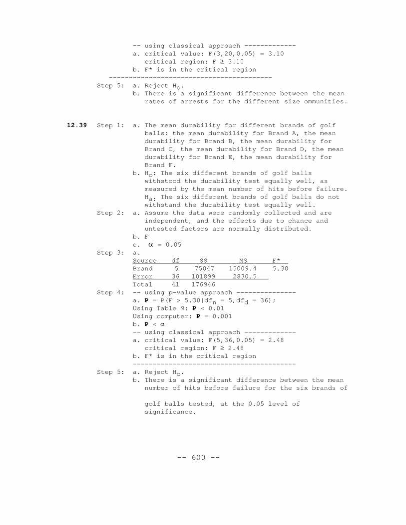
12.39 Step 1: a. The mean durability for different brands of golfballs: the mean durability for Brand A, the meandurability for Brand B, the mean durability forBrand C, the mean durability for Brand D, the meandurability for Brand E, the mean durability forBrand F.
b. Ho: The six different brands of golf ballswithstood the durability test equally well, asmeasured by the mean number of hits before failure.Ha: The six different brands of golf balls do notwithstand the durability test equally well.
Step 2: a. Assume the data were randomly collected and areindependent, and the effects due to chance anduntested factors are normally distributed.
b. Fc. α = 0.05
Step 3: a. Source df SS MS F* Brand 5 75047 15009.4 5.30Error 36 101899 2830.5 Total 41 176946
Step 4: -- using p-value approach ---------------a. P = P(F > 5.30|dfn = 5,dfd = 36);Using Table 9: P < 0.01Using computer: P = 0.001b. P < α-- using classical approach -------------a. critical value: F(5,36,0.05) = 2.48
critical region: F ≥ 2.48b. F* is in the critical region-----------------------------------------
Step 5: a. Reject Ho.b. There is a significant difference between the mean number of hits before failure for the six brands of
golf balls tested, at the 0.05 level ofsignificance.
-- 601 --
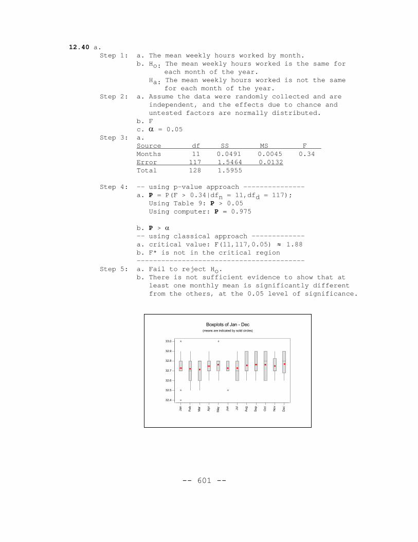
12.40 a.Step 1: a. The mean weekly hours worked by month.
b. Ho: The mean weekly hours worked is the same foreach month of the year.
Ha: The mean weekly hours worked is not the samefor each month of the year.
Step 2: a. Assume the data were randomly collected and areindependent, and the effects due to chance anduntested factors are normally distributed.
b. Fc. α = 0.05
Step 3: a. Source df SS MS F Months 11 0.0491 0.0045 0.34Error 117 1.5464 0.0132Total 128 1.5955
Step 4: -- using p-value approach ---------------a. P = P(F > 0.34|dfn = 11,dfd = 117);
Using Table 9: P > 0.05Using computer: P = 0.975
b. P > α-- using classical approach -------------a. critical value: F(11,117,0.05) ≈ 1.88b. F* is not in the critical region-----------------------------------------
Step 5: a. Fail to reject Ho.b. There is not sufficient evidence to show that at
least one monthly mean is significantly differentfrom the others, at the 0.05 level of significance.
Jan
Fe
b
Mar
Ap
r
May Ju
n
Jul
Aug
Se
p
Oct
No
v
De
c
32.4
32.5
32.6
32.7
32.8
32.9
33.0
Boxplots of Jan - Dec(means are indicated by solid circles)
-- 602 --
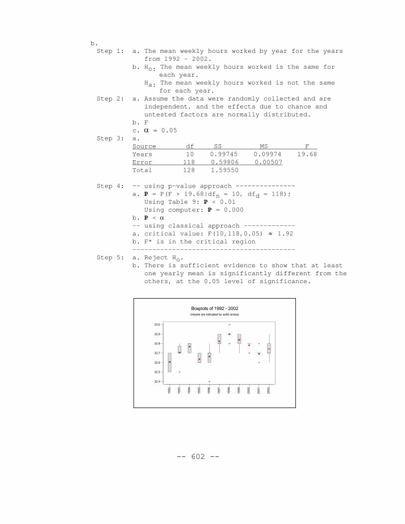
b.Step 1: a. The mean weekly hours worked by year for the years
from 1992 - 2002.b. Ho: The mean weekly hours worked is the same for
each year.Ha: The mean weekly hours worked is not the same
for each year.Step 2: a. Assume the data were randomly collected and are
independent, and the effects due to chance anduntested factors are normally distributed.
b. Fc. α = 0.05
Step 3: a. Source df SS MS F Years 10 0.99745 0.09974 19.68Error 118 0.59806 0.00507Total 128 1.59550
Step 4: -- using p-value approach ---------------a. P = P(F > 19.68|dfn = 10, dfd = 118);
Using Table 9: P < 0.01Using computer: P = 0.000
b. P < α-- using classical approach -------------a. critical value: F(10,118,0.05) ≈ 1.92b. F* is in the critical region-----------------------------------------
Step 5: a. Reject Ho.b. There is sufficient evidence to show that at least
one yearly mean is significantly different from theothers, at the 0.05 level of significance.
19
92
19
93
19
94
19
95
19
96
19
97
19
98
19
99
20
00
20
01
20
02
32.4
32.5
32.6
32.7
32.8
32.9
33.0
Boxplots of 1992 - 2002(means are indicated by solid circles)
-- 603 --
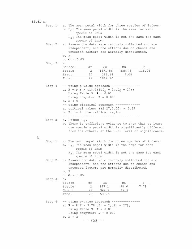
12.41 a.Step 1: a. The mean petal width for three species of irises.
b. Ho: The mean petal width is the same for eachspecie of iris
Ha: The mean petal width is not the same for eachspecie of iris.
Step 2: a. Assume the data were randomly collected and areindependent, and the effects due to chance anduntested factors are normally distributed.
b. Fc. α = 0.05
Step 3: a. Source df SS MS F Specie 2 1671.56 835.78 118.06Error 27 191.14 7.08Total 29 1862.70
Step 4: -- using p-value approach ---------------a. P = P(F > 118.06|dfn = 2,dfd = 27);
Using Table 9: P < 0.01Using computer: P = 0.000
b. P < α-- using classical approach -------------a. critical value: F(2,27,0.05) ≈ 3.37b. F* is in the critical region-----------------------------------------
Step 5: a. Reject Ho.b. There is sufficient evidence to show that at least
one specie’s petal width is significantly differentfrom the others, at the 0.05 level of significance.
b.Step 1: a. The mean sepal width for three species of irises.
b. Ho: The mean sepal width is the same for eachspecie of iris
Ha: The mean sepal width is not the same for eachspecie of iris.
Step 2: a. Assume the data were randomly collected and areindependent, and the effects due to chance anduntested factors are normally distributed.
b. Fc. α = 0.05
Step 3: a. Source df SS MS F Specie 2 197.1 98.6 7.78Error 27 342.2 12.7Total 29 539.4
Step 4: -- using p-value approach ---------------a. P = P(F > 7.78|dfn = 2,dfd = 27);
Using Table 9: P < 0.01Using computer: P = 0.002
b. P < α
-- 604 --
-- using classical approach -------------a. critical value: F(2,27,0.05) ≈ 3.37b. F* is in the critical region-----------------------------------------
Step 5: a. Reject Ho.b. There is sufficient evidence to show that at least
one specie’s sepal width is significantly differentfrom the others, at the 0.05 level of significance.
c. Type 0 has the shortest PW and the longest SW. Type 1 has thelongest PW and the middle SW. Type 2 has the middle PW and theshortest SW.
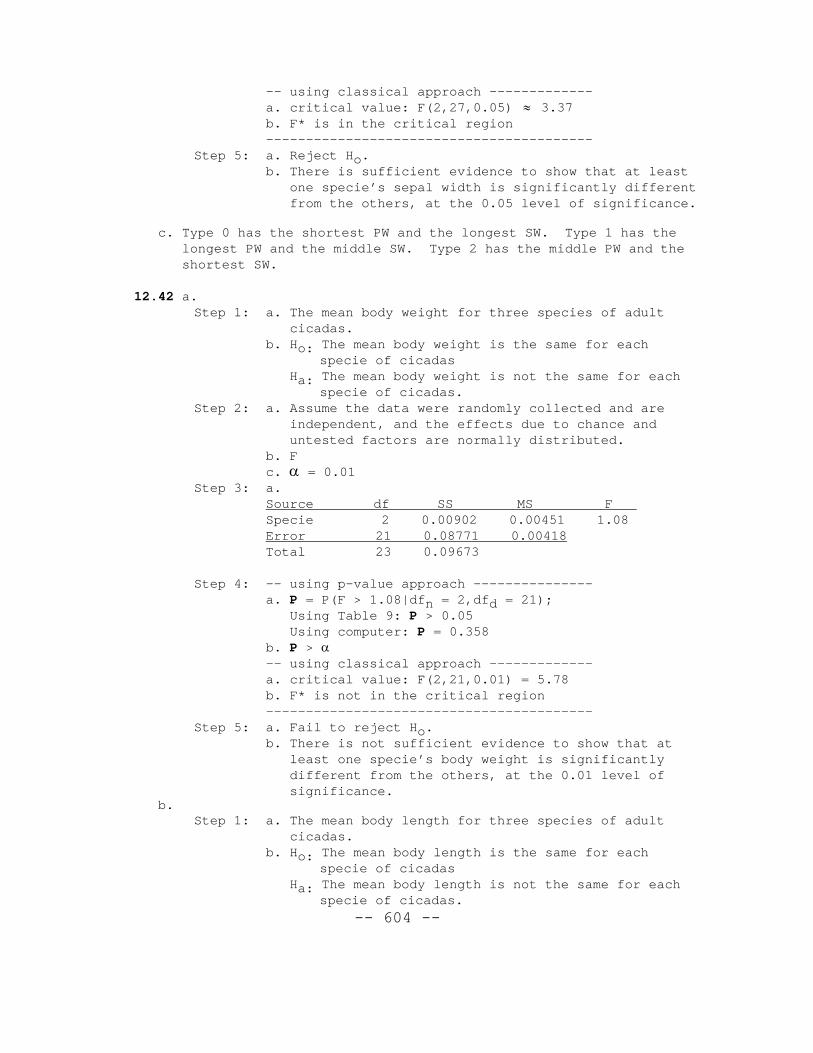
12.42 a.Step 1: a. The mean body weight for three species of adult
cicadas.b. Ho: The mean body weight is the same for each
specie of cicadasHa: The mean body weight is not the same for each
specie of cicadas.Step 2: a. Assume the data were randomly collected and are
independent, and the effects due to chance anduntested factors are normally distributed.
b. Fc. α = 0.01
Step 3: a. Source df SS MS F Specie 2 0.00902 0.00451 1.08Error 21 0.08771 0.00418Total 23 0.09673
Step 4: -- using p-value approach ---------------a. P = P(F > 1.08|dfn = 2,dfd = 21);
Using Table 9: P > 0.05Using computer: P = 0.358
b. P > α-- using classical approach -------------a. critical value: F(2,21,0.01) = 5.78b. F* is not in the critical region-----------------------------------------
Step 5: a. Fail to reject Ho.b. There is not sufficient evidence to show that at
least one specie’s body weight is significantlydifferent from the others, at the 0.01 level ofsignificance.
b.Step 1: a. The mean body length for three species of adult
cicadas.b. Ho: The mean body length is the same for each
specie of cicadasHa: The mean body length is not the same for each
specie of cicadas.
-- 605 --
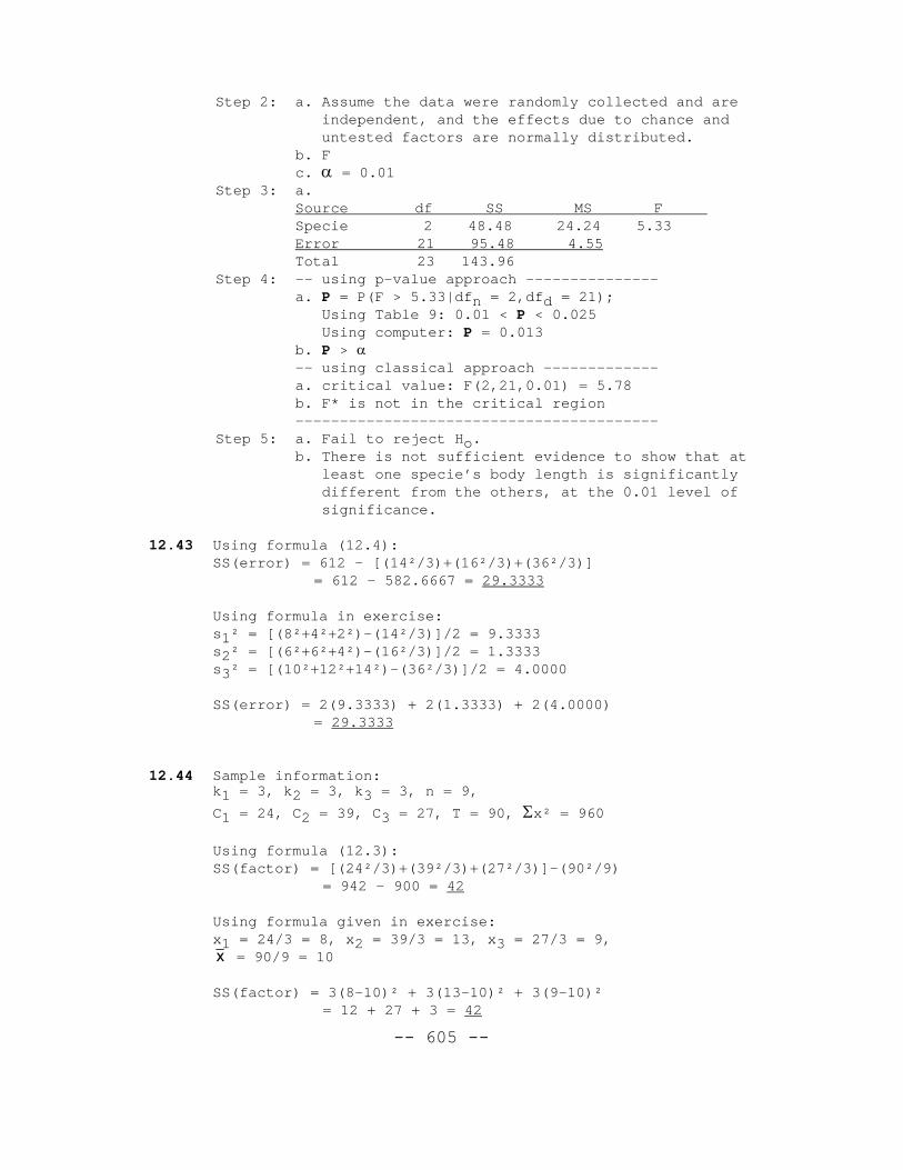
Step 2: a. Assume the data were randomly collected and areindependent, and the effects due to chance anduntested factors are normally distributed.
b. Fc. α = 0.01
Step 3: a. Source df SS MS F Specie 2 48.48 24.24 5.33Error 21 95.48 4.55Total 23 143.96
Step 4: -- using p-value approach ---------------a. P = P(F > 5.33|dfn = 2,dfd = 21);
Using Table 9: 0.01 < P < 0.025Using computer: P = 0.013
b. P > α-- using classical approach -------------a. critical value: F(2,21,0.01) = 5.78b. F* is not in the critical region-----------------------------------------
Step 5: a. Fail to reject Ho.b. There is not sufficient evidence to show that at
least one specie’s body length is significantlydifferent from the others, at the 0.01 level ofsignificance.
12.43 Using formula (12.4):SS(error) = 612 - [(14²/3)+(16²/3)+(36²/3)]
= 612 - 582.6667 = 29.3333
Using formula in exercise:s1² = [(8²+4²+2²)-(14²/3)]/2 = 9.3333s2² = [(6²+6²+4²)-(16²/3)]/2 = 1.3333s3² = [(10²+12²+14²)-(36²/3)]/2 = 4.0000
SS(error) = 2(9.3333) + 2(1.3333) + 2(4.0000) = 29.3333
12.44 Sample information:k1 = 3, k2 = 3, k3 = 3, n = 9,
C1 = 24, C2 = 39, C3 = 27, T = 90, Σx² = 960
Using formula (12.3):SS(factor) = [(24²/3)+(39²/3)+(27²/3)]-(90²/9)
= 942 - 900 = 42
Using formula given in exercise:x1 = 24/3 = 8, x2 = 39/3 = 13, x3 = 27/3 = 9,x = 90/9 = 10
SS(factor) = 3(8-10)² + 3(13-10)² + 3(9-10)² = 12 + 27 + 3 = 42
-- 606 --
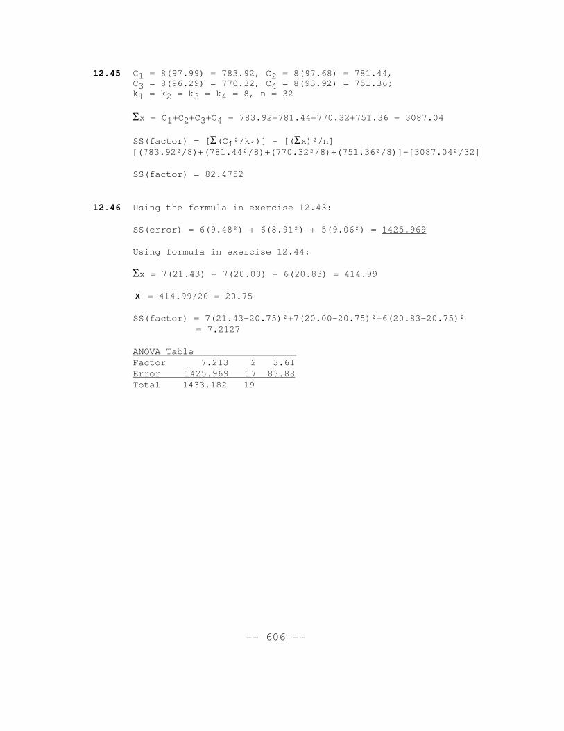
12.45 C1 = 8(97.99) = 783.92, C2 = 8(97.68) = 781.44,C3 = 8(96.29) = 770.32, C4 = 8(93.92) = 751.36;k1 = k2 = k3 = k4 = 8, n = 32
Σx = C1+C2+C3+C4 = 783.92+781.44+770.32+751.36 = 3087.04
SS(factor) = [Σ(Ci²/ki)] - [(Σx)²/n] [(783.92²/8)+(781.44²/8)+(770.32²/8)+(751.36²/8)]-[3087.04²/32]
SS(factor) = 82.4752
12.46 Using the formula in exercise 12.43:
SS(error) = 6(9.48²) + 6(8.91²) + 5(9.06²) = 1425.969
Using formula in exercise 12.44:
Σx = 7(21.43) + 7(20.00) + 6(20.83) = 414.99
x = 414.99/20 = 20.75
SS(factor) = 7(21.43-20.75)²+7(20.00-20.75)²+6(20.83-20.75)²= 7.2127
ANOVA Table Factor 7.213 2 3.61Error 1425.969 17 83.88Total 1433.182 19