1

CHAPTER 13

LAGRANGIAN MECHANICS

13.1 Introduction

The usual way of using newtonian mechanics to solve a problem in dynamics is first of

all to draw a large, clear diagram of the system, using a ruler and a compass. Then mark

in the forces on the various parts of the system with red arrows and the accelerations of

the various parts with green arrows. Then apply the equation F = ma in two different

directions if it is a two-dimensional problem or in three directions if it is a three-

dimensional problem, or θ=τ &&I if torques are involved. More correctly, if a mass or a

moment of inertia is not constant, the equations are pF &= and .L&=τ In any case, we

arrive at one or more equations of motion, which are differential equations which we

integrate with respect to space or time to find the desired solution. Most of us will have

done many, many problems of that sort.

Sometimes it is not all that easy to find the equations of motion as described above.

There is an alternative approach known as lagrangian mechanics which enables us to find

the equations of motion when the newtonian method is proving difficult. In lagrangian

mechanics we start, as usual, by drawing a large, clear diagram of the system, using a

ruler and a compass. But, rather than drawing the forces and accelerations with red and

green arrows, we draw the velocity vectors (including angular velocities) with blue

arrows, and, from these we write down the kinetic energy of the system. If the forces are

conservative forces (gravity, springs and stretched strings), we write down also the

potential energy. That done, the next step is to write down the lagrangian equations of

motion for each coordinate. These equations involve the kinetic and potential energies,

and are a little bit more involved than F = ma, though they do arrive at the same results.

I shall derive the lagrangian equations of motion, and while I am doing so, you will think

that the going is very heavy, and you will be discouraged. At the end of the derivation

you will see that the lagrangian equations of motion are indeed rather more involved than

F = ma, and you will begin to despair – but do not do so! In a very short time after that

you will be able to solve difficult problems in mechanics that you would not be able to

start using the familiar newtonian methods, and the speed at which you do so will be

limited solely by the speed at which you can write. Indeed, you scarcely have to stop and

think. You know straight away what you have to do. Draw the diagram. Mark the

velocity vectors. Write down expressions for the kinetic and potential energies, and

apply the lagrangian equations. It is automatic, fast, and enjoyable.

Incidentally, when Lagrange first published his great work La méchanique analytique

(the modern French spelling would be mécanique), he pointed out with some pride in his

introduction that there were no drawings or diagrams in the book – because all of

mechanics could be done analytically – i.e. with algebra and calculus. Not all of us,

however, are as gifted as Lagrange, and we cannot omit the first and very important step

2

of drawing a large and clear diagram with ruler and compass and marking all the velocity

vectors.

13.2 Generalized Coordinates and Generalized Forces

In two-dimensions the positions of a point can be specified either by its rectangular

coordinates (x, y) or by its polar coordinates. There are other possibilities such as

confocal conical coordinates that might be less familiar. In three dimensions there are the

options of rectangular coordinates (x, y, z), or cylindrical coordinates (ρ, φ, z) or

spherical coordinates (r, θ , φ) – or again there may be others that may be of use for

specialized purposes (inclined coordinates in crystallography, for example, come to

mind). The state of a molecule might be described by a number of parameters, such as

the bond lengths and the angles between the bonds, and these may be varying

periodically with time as the molecule vibrates and twists, and these bonds lengths and

bond angles constitute a set of coordinates which describe the molecule. We are not

going to think about any particular sort of coordinate system or set of coordinates.

Rather, we are going to think about generalized coordinates, which may be lengths or

angles or various combinations of them. We shall call these coordinates (q1 , q2 , q3 ,...).

If we are thinking of a single particle in three-dimensional space, there will be three of

them, which could be rectangular, or cylindrical, or spherical. If there were N particles,

we would need 3N coordinates to describe the system – unless there were some

constraints on the system.

With each generalized coordinate qj is associated a generalized force Pj, which is defined

as follows. If the work required to increase the coordinate qj by δqj is Pj δqj, then Pj is

the generalized force associated with the coordinate qj.

It will be noted that a generalized force need not always be dimensionally equivalent to a

force. For example, if a generalized coordinate is an angle, the corresponding

generalized force will be a torque.

One of the things that we shall want to do is to identify the generalized force associated

with a given generalized coordinate.

13.3 Holonomic constraints

The complete description of a system of N unconstrained particles requires 3N

coordinates. You can think of the state of the system at any time as being represented by

a single point in 3N-dimensional space. If the system consists of molecules in a gas, or a

cluster of stars, or a swarm of bees, the coordinates will be continually changing, and the

point that describes the system will be moving, perhaps completely unconstrained, in its

3N-dimensional space.

3

However, in many systems, the particles may not be free to wander anywhere at will;

they may be subject to various constraints. A constraint that can be described by an

equation relating the coordinates (and perhaps also the time) is called a holonomic

constraint, and the equation that describes the constraint is a holonomic equation. If a

system of N particles is subject to k holonomic constraints, the point in 3N-dimensional

space that describes the system at any time is not free to move anywhere in 3N-

dimensional space, but it is constrained to move over a surface of dimension 3N − k. In

effect only 3N − k coordinates are needed to describe the system, given that the

coordinates are connected by k holonomic equations.

Incidentally, I looked up the word “holonomic” in The Oxford English Dictionary and it

said that the word was from the Greek őλος, meaning “whole” or “entire” and νóµ-ος,

meaning “law”. It also said “applied to a constrained system in which the equations

defining the constraints are integrable or already free of differentials, so that each

equation effectively reduces the number of coordinates by one; also applied to the

constraints themselves.”

As an example, consider a bar of wet soap slithering around in a hemispherical basin of

radius a. You can describe its position in the basin by means of the usual two spherical

angles (θ , φ); the motion is otherwise constrained by its remaining in contact with the

basin; that is to say it is subject to the holonomic constraint r = a. Thus instead of

needing three coordinates to describe the position of a totally unconstrained particle, we

need only two coordinates.

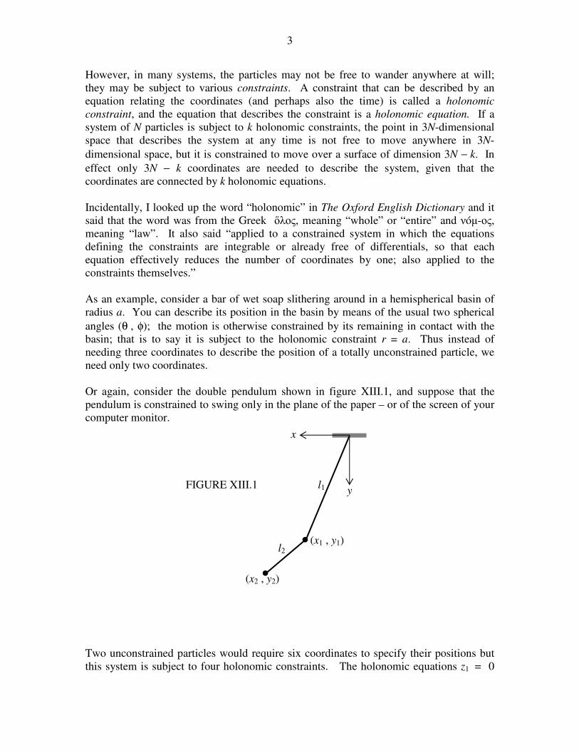
Or again, consider the double pendulum shown in figure XIII.1, and suppose that the

pendulum is constrained to swing only in the plane of the paper – or of the screen of your

computer monitor.

Two unconstrained particles would require six coordinates to specify their positions but

this system is subject to four holonomic constraints. The holonomic equations z1 = 0

l1

l2 •

•

x

y FIGURE XIII.1

(x1 , y1)

(x2 , y2)

4

and z2 = 0 constrain the particles to be moving in a plane, and, if the strings are kept

taut, we have the additional holonomic constraints 2

1

2

1

2

1 lyx =+

and .)()( 2

2

2

12

2

12 lyyxx =−+− Thus only two coordinates are needed to describe the

system, and they could conveniently be the angles that the two strings make with the

vertical.

13.4 The Lagrangian Equations of Motion

This section might be tough – but don’t be put off by it. I promise that, after we have got

over this section, things will be easy. But in this section I don’t like all these summations

and subscripts any more than you do.

Suppose that we have a system of N particles, and that the force on the ith particle (i = 1

to N) is Fi. If the ith particle undergoes a displacement δri, the total work done on the

system is .i

i

i rF δ⋅∑ The position vector r of a particle can be written as a function of its

generalized coordinates; and a change in r can be expressed in terms of the changes in the

generalized coordinates. Thus the total work done on the system is

,j

j j

i

i

i qq

δ∂

∂∑∑ ⋅ r

F 13.4.1

which can be written .∑∑ δ∂

∂⋅j

j

j

i

i

i qq

rF 13.4.2

But by definition of the generalized force, the work done on the system is also

.j

j

j qP δ⋅∑ 13.4.3

Thus the generalized force Pi associated with generalized coordinate qi is given by

.

j

i

i

ijq

P∂

∂= ⋅∑

rF 13.4.4

Now iii m rF &&= , so that

.

j

ii

i

ijq

mP∂

∂= ⋅∑

rr&& 13.4.5

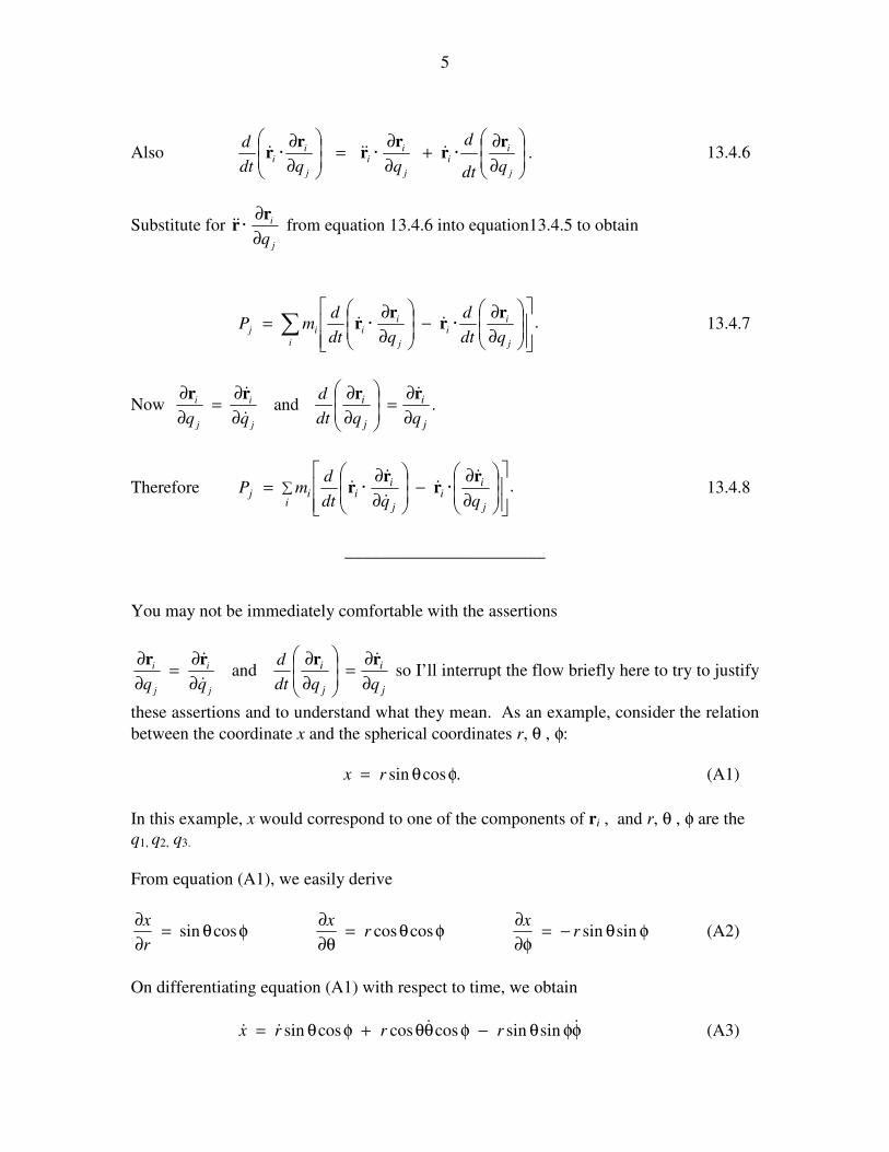
5

Also .

∂

∂+

∂

∂=

∂

∂ ⋅⋅⋅j

ii

j

ii

j

ii

qdt

d

qqdt

d rr

rr

rr &&&& 13.4.6

Substitute for j

i

q∂

∂⋅ rr&& from equation 13.4.6 into equation13.4.5 to obtain

.

∂

∂−

∂

∂= ⋅⋅∑

j

ii

j

ii

i

ijqdt

d

qdt

dmP

rr

rr && 13.4.7

Now j

i

j

i

qq &

&

∂

∂=

∂

∂ rr and .

j

i

j

i

qqdt

d

∂

∂=

∂

∂ rr &

Therefore .

∂

∂−

∂

∂= ⋅⋅∑

j

ii

j

ii

iij

qqdt

dmP

rr

rr

&&

&

&& 13.4.8

_______________________

You may not be immediately comfortable with the assertions

j

i

j

i

qq &

&

∂

∂=

∂

∂ rr and

j

i

j

i

qqdt

d

∂

∂=

∂

∂ rr &so I’ll interrupt the flow briefly here to try to justify

these assertions and to understand what they mean. As an example, consider the relation

between the coordinate x and the spherical coordinates r, θ , φ:

.cossin φθ= rx (A1)

In this example, x would correspond to one of the components of ri , and r, θ , φ are the

q1, q2, q3.

From equation (A1), we easily derive

φθ−=φ∂

∂φθ=

θ∂

∂φθ=

∂

∂sinsincoscoscossin r

xr

x

r

x (A2)

On differentiating equation (A1) with respect to time, we obtain

φφθ−φθθ+φθ= &&&& sinsincoscoscossin rrrx (A3)

6

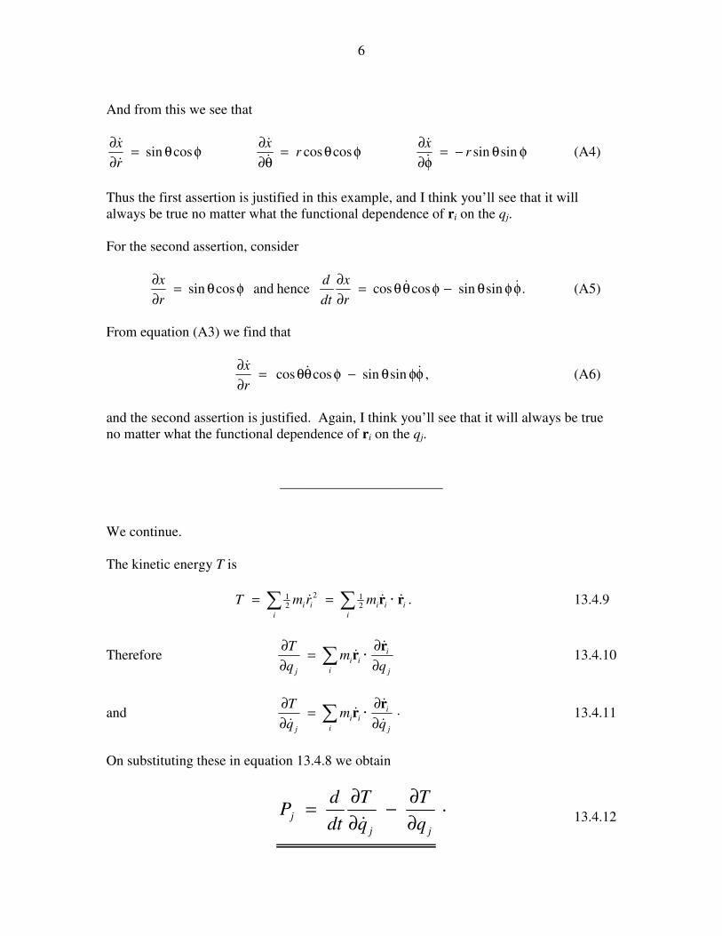
And from this we see that

φθ−=φ∂

∂φθ=

θ∂

∂φθ=

∂

∂sinsincoscoscossin r

xr

x

r

x

&

&

&

&

&

& (A4)

Thus the first assertion is justified in this example, and I think you’ll see that it will

always be true no matter what the functional dependence of ri on the qj.

For the second assertion, consider

.sinsincoscoshence andcossin φφθ−φθθ=∂

∂φθ=

∂

∂&&

r

x

dt

d

r

x (A5)

From equation (A3) we find that

φφθ−φθθ=∂

∂&&

&sinsincoscos

r

x, (A6)

and the second assertion is justified. Again, I think you’ll see that it will always be true

no matter what the functional dependence of ri on the qj.

_______________________

We continue.

The kinetic energy T is

.212

21

i

i

ii

i

ii mrmT rr &&& ⋅∑∑ == 13.4.9

Therefore j

ii

i

i

j qm

q

T

∂

∂=

∂

∂ ⋅∑r

r&

& 13.4.10

and .

j

ii

i

i

j qm

q

T

&

&&

& ∂

∂=

∂

∂ ⋅∑r

r 13.4.11

On substituting these in equation 13.4.8 we obtain

.

jj

jq

T

q

T

dt

dP

∂

∂−

∂

∂=

& 13.4.12

7

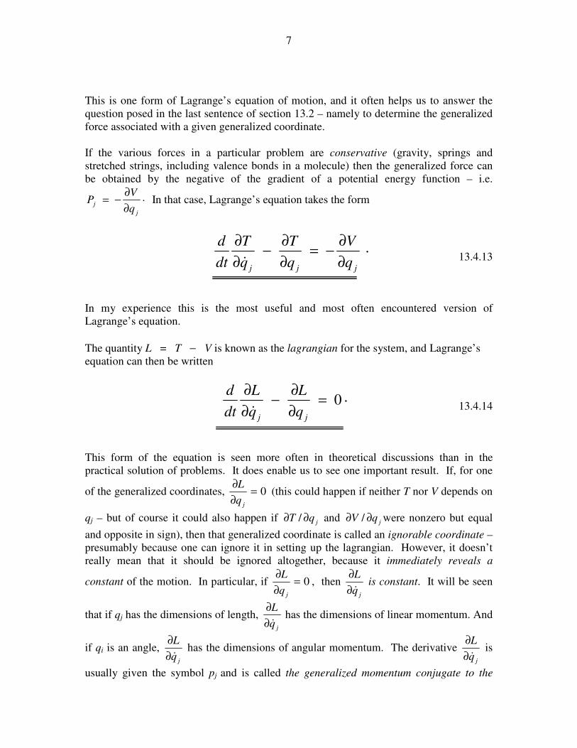
This is one form of Lagrange’s equation of motion, and it often helps us to answer the

question posed in the last sentence of section 13.2 – namely to determine the generalized

force associated with a given generalized coordinate.

If the various forces in a particular problem are conservative (gravity, springs and

stretched strings, including valence bonds in a molecule) then the generalized force can

be obtained by the negative of the gradient of a potential energy function – i.e.

.

j

jq

VP

∂

∂−= In that case, Lagrange’s equation takes the form

.

jjj q

V

q

T

q

T

dt

d

∂

∂−=

∂

∂−

∂

∂

& 13.4.13

In my experience this is the most useful and most often encountered version of

Lagrange’s equation.

The quantity L = T − V is known as the lagrangian for the system, and Lagrange’s

equation can then be written

.0=

∂

∂−

∂

∂

jj q

L

q

L

dt

d

& 13.4.14

This form of the equation is seen more often in theoretical discussions than in the

practical solution of problems. It does enable us to see one important result. If, for one

of the generalized coordinates, 0=∂

∂

jq

L (this could happen if neither T nor V depends on

qj – but of course it could also happen if jqT ∂∂ / and jqV ∂∂ / were nonzero but equal

and opposite in sign), then that generalized coordinate is called an ignorable coordinate –

presumably because one can ignore it in setting up the lagrangian. However, it doesn’t

really mean that it should be ignored altogether, because it immediately reveals a

constant of the motion. In particular, if 0=∂

∂

jq

L, then

jq

L

&∂

∂ is constant. It will be seen

that if qj has the dimensions of length, jq

L

&∂

∂ has the dimensions of linear momentum. And

if qi is an angle, jq

L

&∂

∂ has the dimensions of angular momentum. The derivative

jq

L

&∂

∂ is

usually given the symbol pj and is called the generalized momentum conjugate to the

8

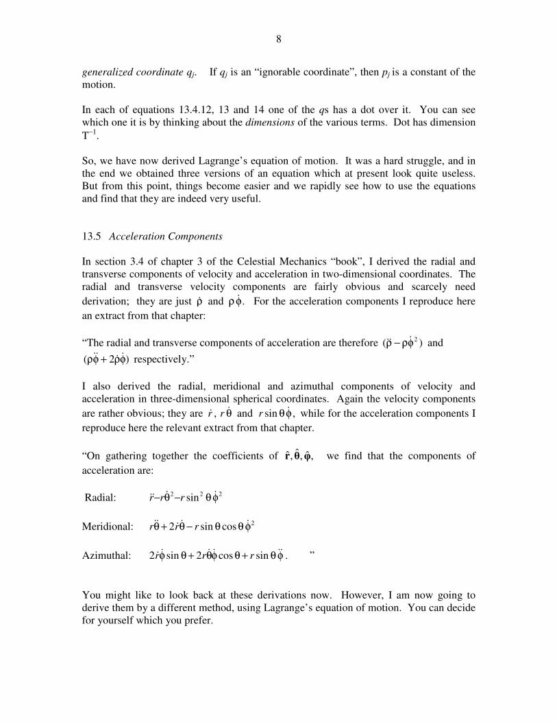
generalized coordinate qj. If qj is an “ignorable coordinate”, then pj is a constant of the

motion.

In each of equations 13.4.12, 13 and 14 one of the qs has a dot over it. You can see

which one it is by thinking about the dimensions of the various terms. Dot has dimension

T−1

.

So, we have now derived Lagrange’s equation of motion. It was a hard struggle, and in

the end we obtained three versions of an equation which at present look quite useless.

But from this point, things become easier and we rapidly see how to use the equations

and find that they are indeed very useful.

13.5 Acceleration Components

In section 3.4 of chapter 3 of the Celestial Mechanics “book”, I derived the radial and

transverse components of velocity and acceleration in two-dimensional coordinates. The

radial and transverse velocity components are fairly obvious and scarcely need

derivation; they are just ρ& and .φρ & For the acceleration components I reproduce here

an extract from that chapter:

“The radial and transverse components of acceleration are therefore )( 2φρ−ρ &&& and

)2( φρ+φρ &&&& respectively.”

I also derived the radial, meridional and azimuthal components of velocity and

acceleration in three-dimensional spherical coordinates. Again the velocity components

are rather obvious; they are ,sinand, φθθ &&& rrr while for the acceleration components I

reproduce here the relevant extract from that chapter.

“On gathering together the coefficients of ,ˆ,ˆ,ˆ φθr we find that the components of

acceleration are:

Radial: 222 sin φθ−θ− &&&& rrr

Meridional: 2cossin2 φθθ−θ+θ &&&&& rrr

Azimuthal: φθ+θφθ+θφ &&&&&& sincos2sin2 rrr . ”

You might like to look back at these derivations now. However, I am now going to

derive them by a different method, using Lagrange’s equation of motion. You can decide

for yourself which you prefer.

9

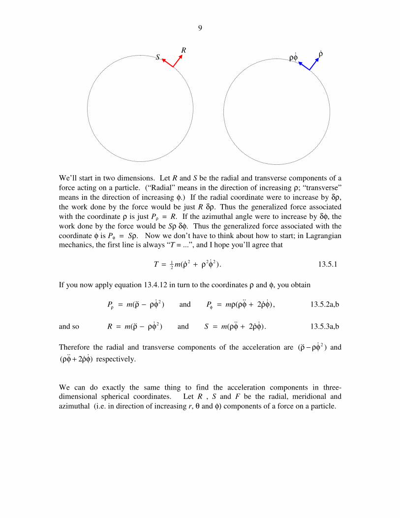
We’ll start in two dimensions. Let R and S be the radial and transverse components of a

force acting on a particle. (“Radial” means in the direction of increasing ρ; “transverse”

means in the direction of increasing φ.) If the radial coordinate were to increase by δρ,

the work done by the force would be just R δρ. Thus the generalized force associated

with the coordinate ρ is just Pρ = R. If the azimuthal angle were to increase by δφ, the

work done by the force would be Sρ δφ. Thus the generalized force associated with the

coordinate φ is Pφ = Sρ. Now we don’t have to think about how to start; in Lagrangian

mechanics, the first line is always “T = ...”, and I hope you’ll agree that

.)( 222

21 φρ+ρ= &&mT 13.5.1

If you now apply equation 13.4.12 in turn to the coordinates ρ and φ, you obtain

,)2(and)( 2 φρ+φρρ=φρ−ρ= φρ&&&&&&& mPmP 13.5.2a,b

and so .)2(and)( 2 φρ+φρ=φρ−ρ= &&&&&&& mSmR 13.5.3a,b

Therefore the radial and transverse components of the acceleration are )( 2φρ−ρ &&& and

)2( φρ+φρ &&&& respectively.

We can do exactly the same thing to find the acceleration components in three-

dimensional spherical coordinates. Let R , S and F be the radial, meridional and

azimuthal (i.e. in direction of increasing r, θ and φ) components of a force on a particle.

R S

ρ& φρ&

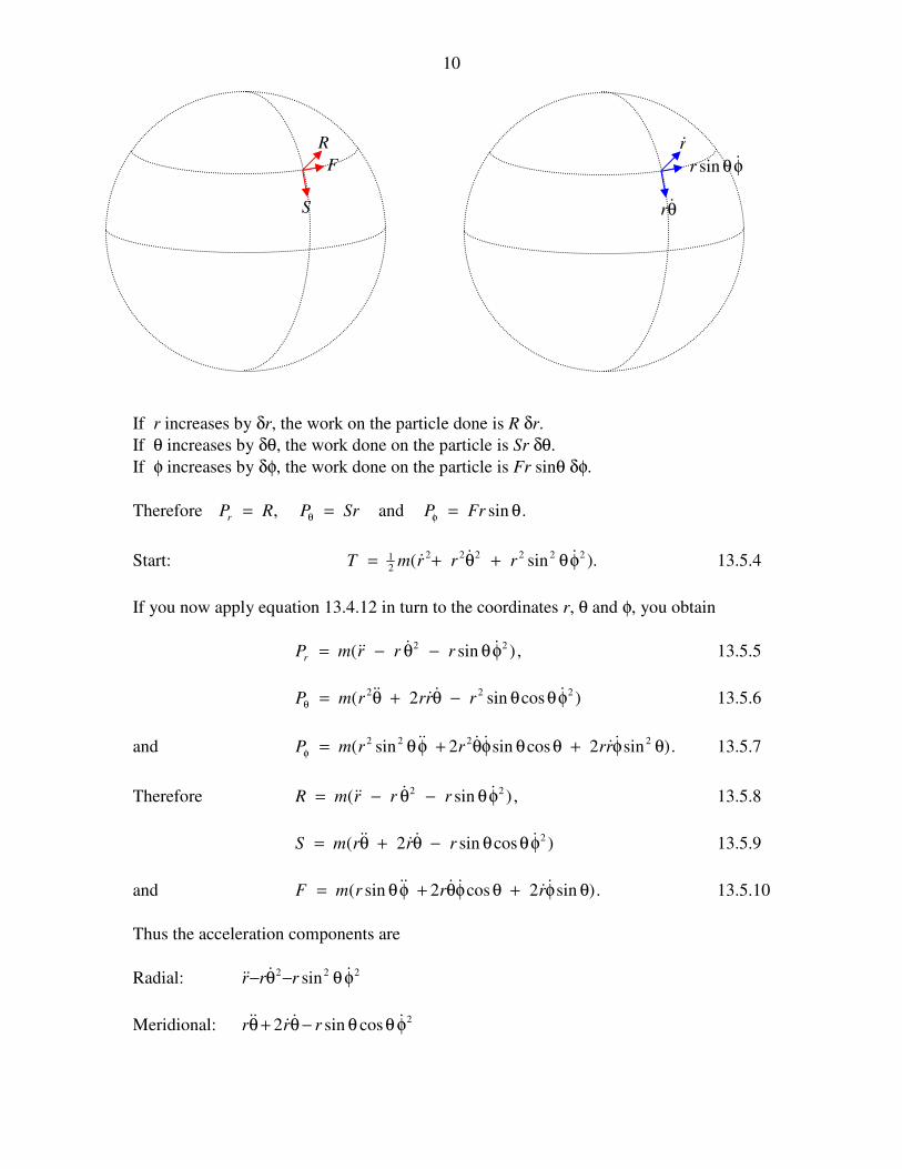
10

If r increases by δr, the work on the particle done is R δr.

If θ increases by δθ, the work done on the particle is Sr δθ.

If φ increases by δφ, the work done on the particle is Fr sinθ δφ.

Therefore .sinand, θ=== φθ FrPSrPRPr

Start: ).sin( 222222

21 φθ+θ+= &&& rrrmT 13.5.4

If you now apply equation 13.4.12 in turn to the coordinates r, θ and φ, you obtain

,)sin( 22 φθ−θ−= &&&& rrrmPr 13.5.5

)cossin2( 222 φθθ−θ+θ=θ&&&&& rrrrmP 13.5.6

and .)sin2cossin2sin( 2222 θφ+θθφθ+φθ=φ&&&&&& rrrrmP 13.5.7

Therefore ,)sin( 22 φθ−θ−= &&&& rrrmR 13.5.8

)cossin2( 2φθθ−θ+θ= &&&&& rrrmS 13.5.9

and .)sin2cos2sin( θφ+θφθ+φθ= &&&&&& rrrmF 13.5.10

Thus the acceleration components are

Radial: 222 sin φθ−θ− &&&& rrr

Meridional: 2cossin2 φθθ−θ+θ &&&&& rrr

R

S

F

r&

θ&r

φθ &sinr

11

Azimuthal: φθ+θφθ+θφ &&&&&& sincos2sin2 rrr .

Be sure to check the dimensions. Since dot has dimension T−1

, and these expressions

must have the dimensions of acceleration, there must be an r and two dots in each term.

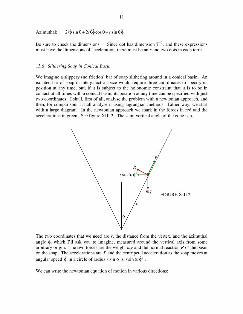
13.6 Slithering Soap in Conical Basin

We imagine a slippery (no friction) bar of soap slithering around in a conical basin. An

isolated bar of soap in intergalactic space would require three coordinates to specify its

position at any time, but, if it is subject to the holonomic constraint that it is to be in

contact at all times with a conical basin, its position at any time can be specified with just

two coordinates. I shall, first of all, analyse the problem with a newtonian approach, and

then, for comparison, I shall analyse it using lagrangian methods. Either way, we start

with a large diagram. In the newtonian approach we mark in the forces in red and the

accelerations in green. See figure XIII.2. The semi vertical angle of the cone is α.

The two coordinates that we need are r, the distance from the vertex, and the azimuthal

angle φ, which I’ll ask you to imagine, measured around the vertical axis from some

arbitrary origin. The two forces are the weight mg and the normal reaction R of the basin

on the soap. The accelerations are r&& and the centripetal acceleration as the soap moves at

angular speed φ& in a circle of radius r sin α is 2sin φα &r .

We can write the newtonian equation of motion in various directions:

•

α

R

mg

r&&

2sin φα &r

FIGURE XIII.2

r

12

Horizontal: )sinsin(cos 2 α−φα=α rrmR &&&

i.e. .)(tan 2 rrmR &&& −φα= 13.6.1

Vertical: .cossin α=−α rmmgR && 13.6.2

Perpendicular

to surface: .cossinsin 2φαα=α− &mrmgR 13.6.3

Parallel

to surface: .sincos 22 rrg &&& −φα=α 13.6.4

Only two of these are independent, and we can choose to use whichever two we want to

at our convenience. There are, however, three quantities that we may wish to determine,

namely the two coordinates r and φ, and the normal reaction R. Thus we need another

equation. We note that, since there are no azimuthal forces, the angular momentum per

unit mass, which is ,sin 22 φα &r is conserved, and therefore φ&2r is constant and equal to

its initial value, which I’ll call l2Ω. That is, we start off at a distance l from the vertex

with an initial angular speed Ω. Thus we have as our third independent equation

.22 Ω=φ lr & 13.6.5

This last equation shows that ∞→φ& as .0→r

One possible type of motion is circular motion at constant height (put 0=r&& ). From

equations 13.6.1 and 2 it is easily found that the condition for this is that

.tansin

2

αα=φ

gr& 13.6.6

In other words, if the particle is projected initially horizontally ( 0=r& ) at r = l and

Ω=φ& , it will describe a horizontal circle (for ever) if

.say,tansin

C

2/1

Ω=

αα=Ω

l

g 13.6.7

13

If the initial speed is less than this, the particle will describe an elliptical orbit with a

minimum r < l; if the initial speed is greater than this, the particle will describe an

elliptical orbit with a maximum r > l.

Now let’s do the same problem in a lagrangian formulation. This time we draw the same

diagram, but we mark in the velocity components in blue. See figure XIII.3. We are

dealing with conservative forces, so we are going to use equation 13.4.13, the most useful

form of Lagrange’s equation.

We need not spend time wondering what to do next. The first and second things we

always have to do are to find the kinetic energy T and the potential energy V, in order that

we can use equation 13.4.13.

)sin( 2222

21 φα+= && rrmT 13.6.8

and constant.cos +α= mgrV 13.6.9

Now go to equation 13.4.13, with qi = r, and work out all the derivatives, and you should

get, when you apply the lagrangian equation to the coordinate r:

.cossin 22 α−=φα− grr &&& 13.6.10

φα &sinr

α

r&

FIGURE XIII.3

r

⊗

14

Now do the same thing with the coordinate φ. You see immediately that φ∂

∂

φ∂

∂ VTand

are both zero. Therefore φ∂

∂&

T

dt

d is zero and therefore

φ∂

∂&

T is constant. That is,

φα &22 sinmr is constant and so φ&2r is constant and equal to its initial value l2Ω. Thus

the second lagrangian equation is

.22 Ω=φ lr & 13.6.11

Since the lagrangian is independent of φ, φ is called, in this connection, an “ignorable

coordinate” – and the momentum associated with it, namely ,2φ&mr is constant.

Now it is true that we arrived at both of these equations also by the newtonian method,

and you may not feel we have gained much. But this is a simple, introductory example,

and we shall soon appreciate the power of the lagrangian method,

Having got these two equations, whether by newtonian or lagrangian methods, let’s

explore them further. For example, let’s eliminate φ& between them and hence get a

single equation in r:

.cossin3

224

α−=αΩ

− gr

lr&& 13.6.12

We know enough by now (see Chapter 6) to write rdr

dr &&& =v

vv where,as , and if we

let the constants αΩ 224 sinl and g cos α equal A and B respectively, equation 13.6.12

becomes

.3

Br

A

dr

d−=

vv 13.6.13

(It may just be useful to note that the dimensions of A and B are L4T

−2 and LT

−2

respectively. This will enable us to keep track of dimensional analysis as we go.)

If we start the soap moving horizontally (v = 0) when r = l, this integrates, with these

initial conditions, to

.)(211

22

2rlB

rlA −+

−=v 13.6.14

15

Again, so that we can see what we are doing, let CBll

A=+ 2

2 (note that [C] = L

2T

−2),

and equation13.6.14 becomes

.22

2Br

r

AC −−=v 13.6.15

This gives )( r&=v as a function of r. The particle reaches is maximum or minimum

height when v = 0; that is where

.02 23 =+− ACrBr 13.6.16

One solution of this is obviously r = l. Of the other two solutions, one is positive (which

we want) and the other is negative (which we don’t want).

If we go back to the original meanings of A, B and C, and write ,/ lrx = equation (16)

becomes, after a little tidying up

.02

tansin1

2

tansin 22

23 =

ααΩ+

+

ααΩ−

g

lx

g

lx 13.6.17

Recall from equation 13.6.7 that

2/1

ctansin

αα=Ω

l

g, and the equation becomes

,02

12 2

c

22

2

c

23 =

Ω

Ω+

+

Ω

Ω− xx 13.6.18

or, with ,2 2

c

2

Ω

Ω=a

( ) .01 23 =++− axax 13.6.19

This factorizes to

.0))(1( 2 =−−− aaxxx 13.6.20

The solution we are interested in is

( ).)4(21 ++= aaax 13.6.21

16

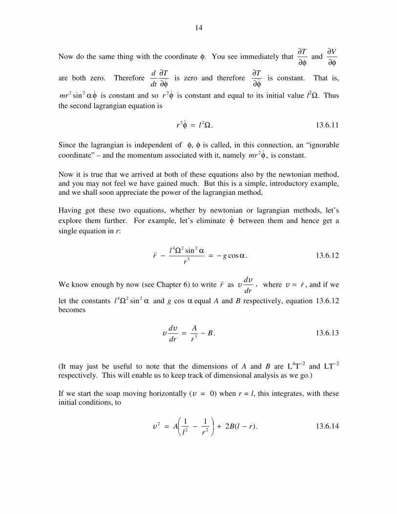
0 0.5 1 1.5 2 2.50

0.5

1

1.5

2

2.5

3

3.5

4

Ω /Ωc

r/l (low

er

or

upper

bound)

13.7 Slithering Soap in Hemispherical Basin

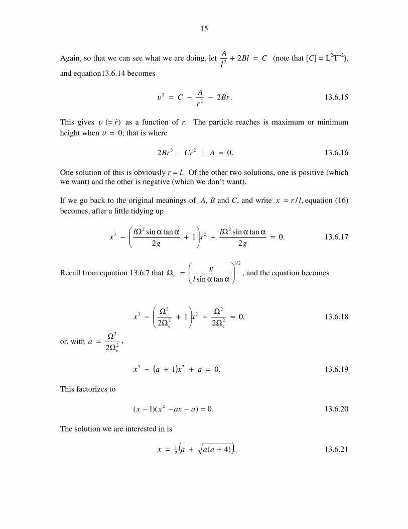
Suppose that the basin is of radius a and the soap is subject to the holonomic constraint r

= a - i.e. that it remains in contact with the basin at all times. Note also that this is just

the same constraint of a pendulum free to swing in three-dimensional space except that it

is subject to the holonomic constraint that the string be taut at all times. Thus any

conclusions that we reach about our soap will also be valid for a pendulum.

We’ll start with the newtonian approach, and I’ll draw in red the two forces on the soap,

namely its weight and the normal reaction of the basin on the soap. Figure XIII.4

FIGURE XIII.4

•

mg

R

θ

17

We’ll make use of the expressions for the radial, meridional and azimuthal accelerations

from section 13.5 and we’ll write down the equations of motion in these directions:

Radial: mg cos θ − R = m( 222 sin φθ−θ− &&&& rrr ), 13.7.1

Meridional: −mg sin θ = m( 2cossin2 φθθ−θ+θ &&&&& rrr ), 13.7.2

Azimuthal: 0 = m( φθ+θφθ+θφ &&&&&& sincos2sin2 rrr ). 13.7.3

We also have the constraint that r = a and hence that ,0== rr &&& after which these

equations become

,)sin(cos 222 φθ+θ−=−θ &&maRmg 13.7.4

,)cossin(sin 2φθθ−θ=θ− &&&ag 13.7.5

.cos2sin0 θφθ+φθ= &&&& 13.7.6

These, then, are the newtonian equations of motion. If you still prefer the newtonian

method to the lagrangian method, and you wish to integrate these and find expressions

θ, φ and R separately, by all means go ahead and do so – but I’m now going to try the

lagrangian approach.

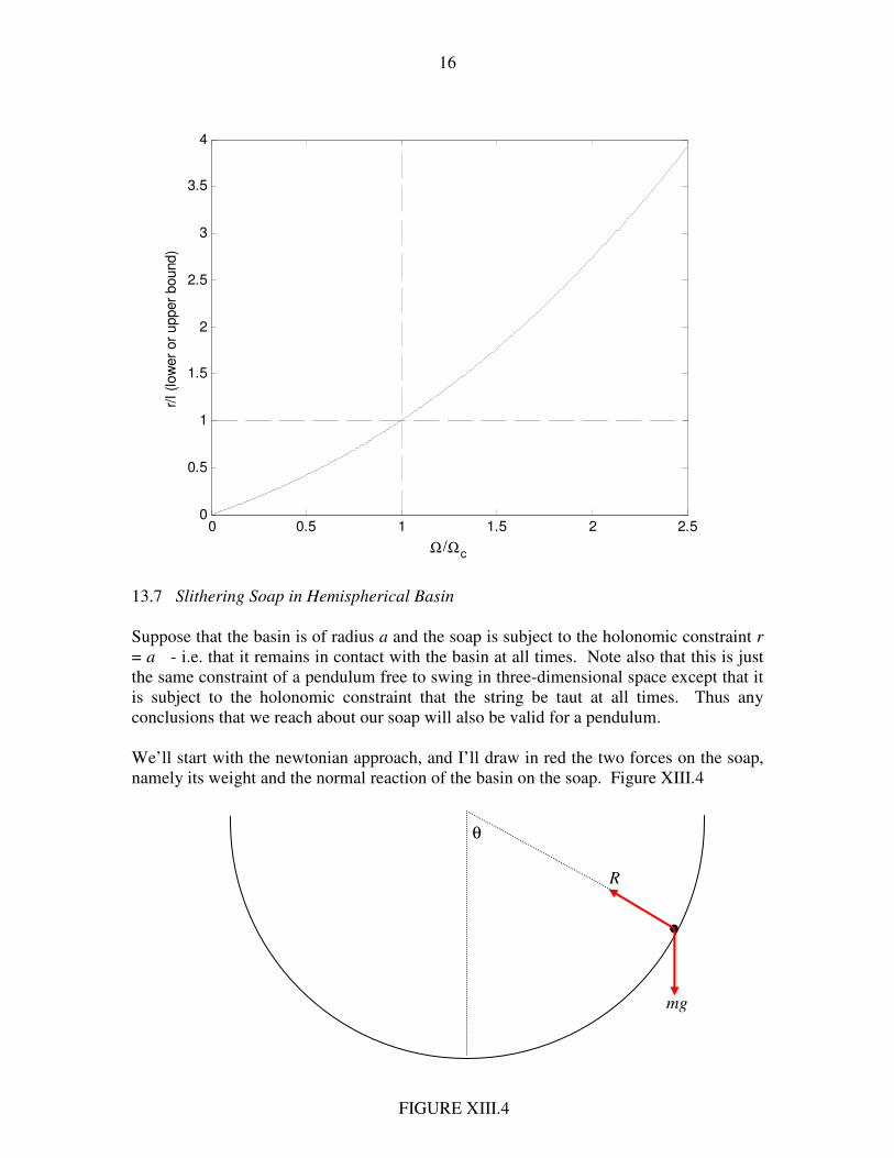
Although Lagrange himself would not have drawn a diagram, we shall not omit that step

– but instead of marking in the forces, we’ll mark in the velocity components, and then

we’ll immediately write down expressions for the kinetic and potential energies. Indeed

the first line of a lagrangian calculation is always “T = ...”.

FIGURE XIII.5

θ

⊗

θ&a

φθ &sina

18

.)sin( 2222

21 φθ+θ= &&maT 13.7.7

.constantcos +θ−= mgaV 13.7.8

Now apply equation 13.4.13 in turn to the coordinates θ and φ.

θ: .sincossin 2 θ−=φθθ−θ gaa &&& 13.7.9

φ: As for the conical basin, we see that φ∂

∂

φ∂

∂ VTand are both zero (φ is an "ignorable

coordinate") and therefore φ∂

∂&

Tis constant and equal to its initial value. If the initial

values of φ& and θ are Ω and α respectively, then

.sinsin 22 Ωα=φθ & 13.7.10

This is merely stating that angular momentum is conserved.

We can easily eliminate φ& from equations 13.4.9 and 10 to obtain

,sin

csccot 2

a

gk

θ−θθ=θ&& 13.7.11

where .sin 24 Ωα=k 13.7.12

Write θ

θθθ

d

d&&&& as in the usual way and integrate to obtain the first space integral:

).csc(csc)cos(cos2 222 α−θ−α−θ=θ ka

g& 13.7.13

The upper and lower bounds for θ occur when .0=θ&

Example. Suppose that the initial value of θ is α = 45o and that we start by pushing the

soap horizontally ( 0=θ& ) at an initial angular speed Ω = 3 rad s−1

, so that k = 2.25 rad2

s−2

. Suppose that the radius of the basin is a = 1.96 m and that g = 9.8 m s−2

. You can

then put 0=θ& in equation 13.7.13 and solve it for θ. One solution, of course, is θ =

α. We could find the other solution by Newton-Raphson iteration, or by putting

)cos1/(1csc 22 θ−=θ and solving it as a cubic equation in cos θ. Alternatively, try

this:

19

Let ,cos,cos,2

cxng

ak=α=θ=

so that .)1/(1cscand)1/(1csc 2222 cx −=α−=θ

The equation then becomes a quadratic equation in x, with solution

That is, .)1(2

]1)()[1(42

22

c

cnccnnx

−

−+−−+−=

I’ll leave you to re-write this in terms of what these quantities originally meant.

13.8 More Examples

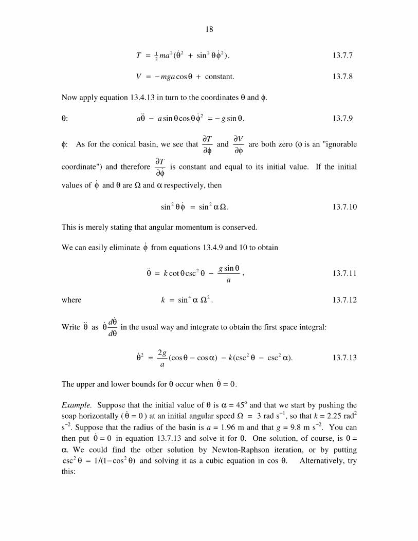
i.

The kinetic energy is .)()( 2

2212

1212

21 yxmyxmxMT &&&&& ++−+= 13.8.1

yx && −

yx && +

x&

M

m1 •

• m2

FIGURE XIII.6

The upper pulley is fixed in position. Both

pulleys rotate freely without friction about their

axles. Both pulleys are “light” in the sense that

their rotational inertias are small and their

rotation contributes negligibly to the kinetic

energy of the system. The rims of the pulleys

are rough, and the ropes do not slip on the

pulleys. The gravitational acceleration is g.

The mass M moves upwards at a rate x& with

respect to the upper, fixed, pulley, and the

smaller pulley moves downwards at the same

rate. The mass m1 moves upwards at a rate

y& with respect to the small pulley, and

consequently its speed in laboratory space is

yx && − . The speed of the mass m2 is therefore

yx && + in laboratory space. The object is to find

x&& and y&& in terms of g.

20

The potential energy is .constant)]()([ 21 ++−−−= yxmyxmMxgV 13.8.2

Apply Lagrange’s equation (13.4.13) in turn to the coordinates x and y:

x: .)()()( 2121 mmMgyxmyxmxM −−−=++−+ &&&&&&&&&& 13.8.3

y: .)()()( 2121 mmgyxmyxm −−=++−− &&&&&&&& 13.8.4

These two equations can be solved at one’s leisure for x&& and .y&&

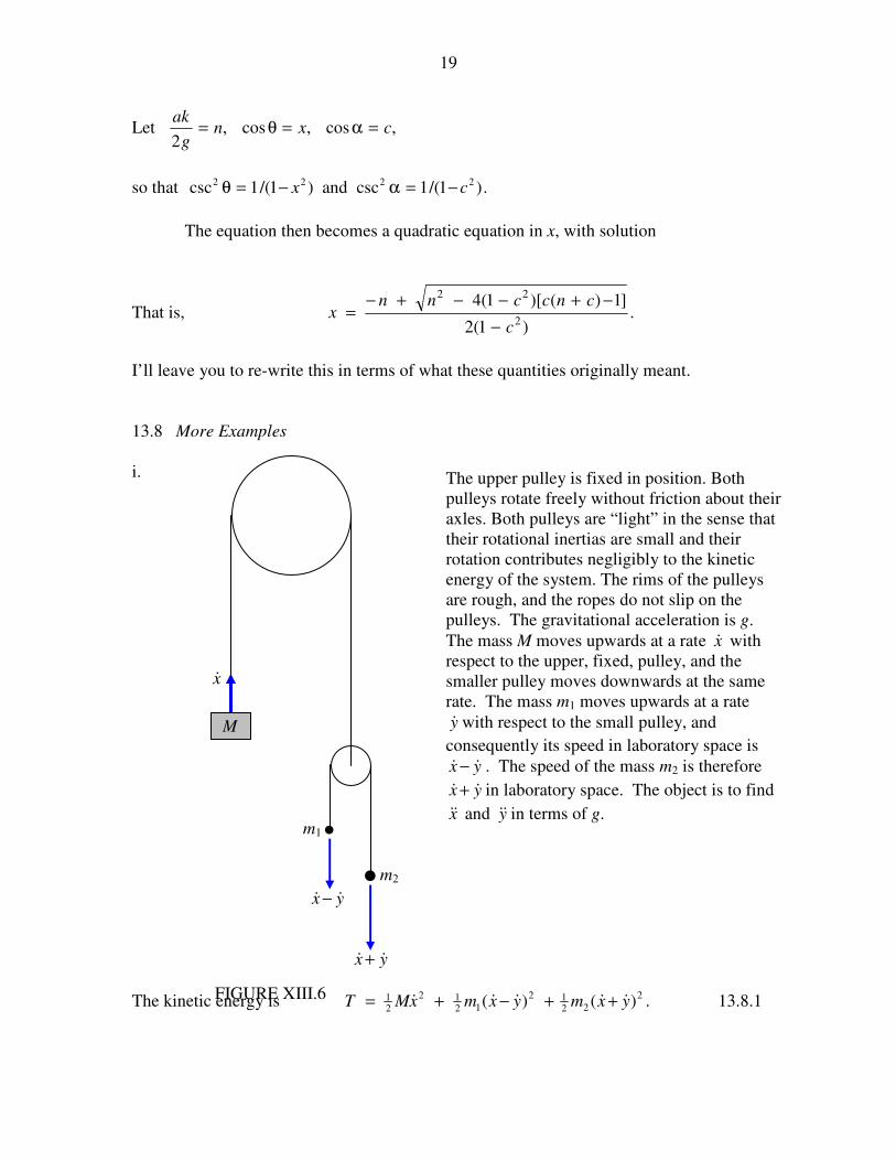
ii. A torus of mass M and radius a rolls without slipping on a horizontal plane. A pearl

of mass m slides smoothly around inside the torus. Describe the motion.

I have marked in the several velocity vectors. The torus is rolling at angular speed .φ&

Consequently the linear speed of the centre of mass of the hoop is ,φ&a and the pearl also

shares this velocity. In addition, the pearl is sliding relative to the torus at an angular

speed θ& and consequently has a component to its velocity of θ&a tangential to the torus.

We are now ready to start.

The kinetic energy of the torus is the sum of its translational and rotational kinetic

energies:

•

θ

φ&a

φ&

θ&a

φ&a

21

.)()( 2222

212

21 φ=φ+φ &&& MaMaaM

The kinetic energy of the pearl is

.)cos2( 222

21 θφθ−φ+θ &&&&ma

Therefore .)cos2( 222

2122 θφθ−φ+θ+φ= &&&&& maMaT 13.8.5

The potential energy is

V = constant − mga cos θ . 13.8.6

The lagrangian equation in θ becomes

.0sin)cos( =θ+θφ−θ ga &&&& 13.8.7

The lagrangian equation in φ becomes

.)sincos()2( 2 θθ−θθ=φ+ &&&&& mmM 13.8.8

These, then, are two differential equations in the two variables. The lagrangian part of

the analysis is over; we now have to see if we can do anything with these equations.

It is easy to eliminate φ&& and hence get a single differential equation in θ:

0sin)2(cossin)sin2( 22 =θ++θθθ+θθ+ gmMmaamM &&& . 13.8.9

If you are good at differential equations, you might be able to do something with this, and

get θ as a function of the time. In the meantime, I think I can get the “first space

integral” (see Chapter 6) – i.e. θ& as a function of θ. Thus, the total energy is constant:

.cos)cos2( 222

2122

EmgamaMa =θ−θφθ−φ+θ+φ &&&&& 13.8.10

Here I am measuring the potential energy from the centre of the circle. Also, if we

assume that the initial condition is that at time t = 0 the kinetic energy was zero and θ =

α, then .cosα−= mgaE

Equation 13.8.8 can easily be integrated once with respect to time, since

,)cos(sincos 2 θθ=θθ−θθ &&&&

dt

d as would have been apparent during the derivation of

22

equation 13.8.8. With the condition that the kinetic energy was initially zero, integration

of equation13.8.8 gives

.cos)2( θθ=φ+ && mmM 13.8.11

Now we can easily eliminate φ& between equations 13.8.10 and 11, to obtain a single

equation relating θ& and θ:

,01cos)sin1( 22 =−θ−θ+θ dcb& 13.8.12

where .sec,2

,)2(

2

α−===+

=E

mgad

M

mc

EmM

Mmab 13.8.13a,b,c

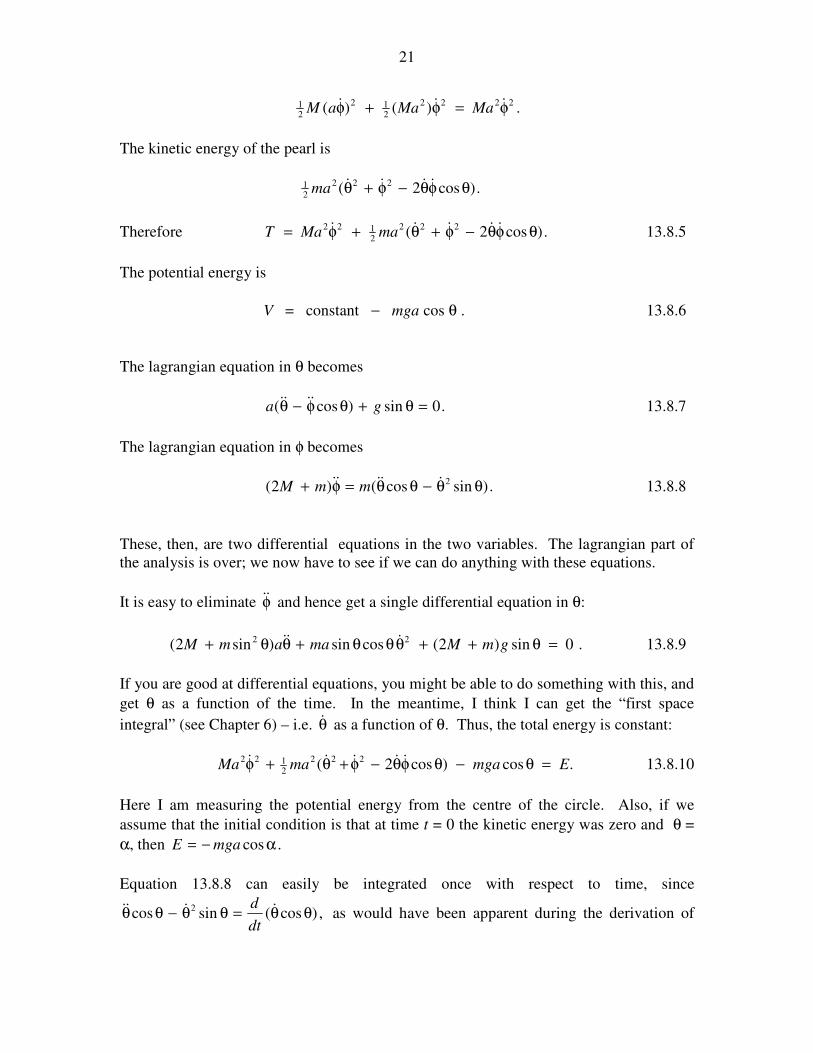
iii.

As in example ii, we have a torus of radius a and mass M, and a pearl of mass m which

can slide freely and without friction around the torus. This time, however, the torus is not

rolling along the table, but is spinning about a vertical axis at an angular speed φ& . The

pearl has a velocity component θ&a because it is sliding around the torus, and a

component φθ &sina because the torus is spinning. The resultant speed is the orthogonal

sum of these. The kinetic energy of the system is the sum of the translational kinetic

energy of the pearl and the rotational kinetic energy of the torus:

.)()sin( 22

21

212222

21 φ+φθ+θ= &&& MamaT 13.8.14

•

θ

φ&

θsina φθ&sina ⊗

θ&a

23

If we refer potential energy to the centre of the torus:

.cosθ= mgaV 13.8.15

The lagrangian equations with respect to the two variables are

θ: .0sin)cossin( 2 =θ−φθθ−θ ga &&& 13.8.16

φ: .constantsin212 =φ+φθ && Mm 13.8.17

The constant is equal to whatever the initial value of the left hand side was. E.g., maybe

the initial values of θ and φ& were α and ω. This finishes the lagrangian part of the

analysis. The rest is up to you. For example, it would be easy to eliminate φ& between

these two equations to obtain a differential equation between θ and the time. If you then

write θθθθ dd /as &&&& in the usual way, I think it wouldn’t be too difficult to obtain the first

space integral and hence get θ& as a function of θ. I haven’t tried it, but I’m sure it’ll

work.

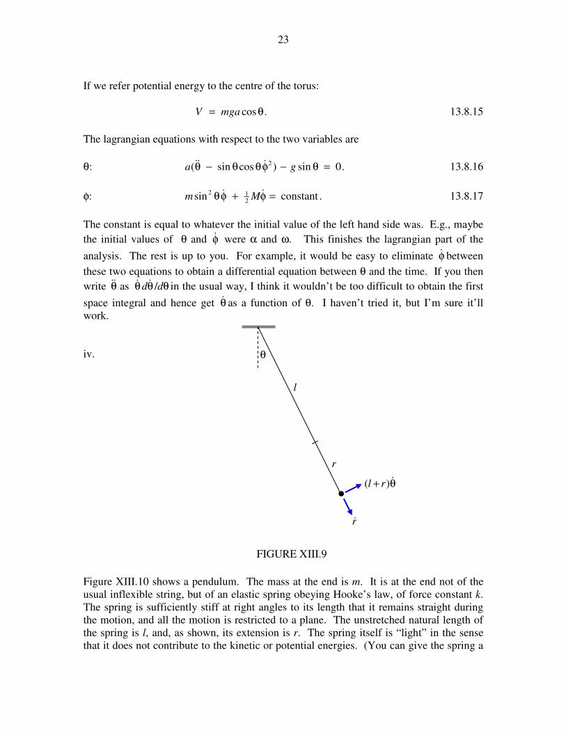
iv.

Figure XIII.10 shows a pendulum. The mass at the end is m. It is at the end not of the

usual inflexible string, but of an elastic spring obeying Hooke’s law, of force constant k.

The spring is sufficiently stiff at right angles to its length that it remains straight during

the motion, and all the motion is restricted to a plane. The unstretched natural length of

the spring is l, and, as shown, its extension is r. The spring itself is “light” in the sense

that it does not contribute to the kinetic or potential energies. (You can give the spring a

θ+ &)( rl

θ

l

r

•

r&

FIGURE XIII.9

24

finite mass if you want to make the problem more difficult.) The kinetic and potential

energies are

( )222

21 )( θ++= && rlrmT 13.8.18

and .cos)(constant 2

21 krrlmgV +θ+−= 13.8.19

Apply Lagrange’s equation in turn to r and to θ and see where it leads you.

v. Another example suitable for lagrangian methods is given as problem number 11 in

Appendix A of these notes.

Lagrangian methods are particularly applicable to vibrating systems, and examples of

these will be discussed in chapter 17. These chapters are being written in more or less

random order as the spirit moves me, rather than in logical order, so that vibrating

systems appear after the unlikely sequence of relativity and hydrostatics.

13.9 Hamilton’s Variational Principle

Hamilton’s variational principle in dynamics is slightly reminiscent of the principle of

virtual work in statics, discussed in section 9.4 of Chapter 9. When using the principle of

virtual work in statics we imagine starting from an equilibrium position, and then

increasing one of the coordinates infinitesimally. We calculate the virtual work done and

set it to zero. I am slightly reminded of this when discussing Hamilton’s principle in

dynamics

Imagine some mechanical system – some contraption including in its construction

various wheels, jointed rods, springs, elastic strings, pendulums, inclined planes,

hemispherical bowls, and ladders leaning against smooth vertical walls and smooth

horizontal floors. It may require N generalized coordinates to describe its configuration

at any time. Its configuration could be described by the position of a point in N-

dimensional space. Or perhaps it is subject to k holonomic constraints – in which case

the point that describes its configuration in N-dimensional space is not free to move

anywhere in that space, but is constrained to slither around on a surface of dimension

.kN −

The system is not static, but it is evolving. It is changing from some initial state at time t1

to some final state at time t2. The generalized coordinates that describe it are changing

with time – and the point in N-space is slithering round on its surface of dimension N − k.

One can imagine that at any instant of time one can calculate its kinetic energy T and its

potential energy V, and hence its lagrangian L = T − V. You can multiply L at some

25

moment by a small time interval δt and then add up all of these products between t1 and t2

to form the integral

∫2

1

.t

tdtL

This quantity – of dimension ML2T

−1 and SI unit J s – is sometimes called the “action”.

There are many different ways in which we can imagine the system to evolve from its

initial state to its final state – and there are many different routes that we can imagine

might be taken by our point in N-space as its moves from its initial position to its final

position, as long as it moves over its surface of dimension N − k. But, although we can

imagine many such routes, the manner in which the system will actually evolve, and the

route that the point will actually take is determined by Hamilton’s principle; and the

route, according to this principle, is such that the integral ∫2

1

t

tdtL is a minimum, or a

maximum, or an inflection point, when compared with other imaginable routes. Stated

otherwise, let us suppose that we calculate ∫2

1

t

tdtL over the actual route taken and then

calculate the variation in ∫2

1

t

tdtL if the system were to move over a slightly different

adjacent path. Then (and here is the analogy with the principle of virtual work in a statics

problem) this variation

∫δ2

1

t

tdtL

from what ∫2

1

t

tdtL would have been over the actual route is zero. And this is Hamilton’s

variational principle.

The next questions will surely be: Can I use this principle for solving problems in

mechanics? Can I prove this bald assertion?

Let me try to use the principle to solve two simple and familiar problems, and then move

on to a more general problem.

The first problem will be this. Imagine that we have a particle than can move in one

dimension (i.e. one coordinate – for example its height y above a table − suffices to

describe its position), and that when its coordinate is y its potential energy is

V = mgy. 13.9.1

Its kinetic energy is, of course,

.2

21 ymT &= 13.9.2

26

We are going to use the variational principle to find the equation of motion – i.e we are

going to find an expression for its acceleration. I imagine at the moment you have no

idea what its acceleration could possibly be – but don’t worry, for we know that the

lagrangian is

,2

21 mgyymL −= & 13.9.3

and we’ll make short work of it with Hamilton’s variational principle and soon find the

acceleration. According to this principle, y must vary with t in such a manner that

∫ =−δ2

1

.0)( 2

21

t

tdtgyym & 13.9.4

Let us vary ,byandby yyyy δδ&& and see how the integral varies.

The integral is then ∫ δ−δ2

1

,)(t

tdtygyym && 13.9.5

which I’ll call I1 − I2.

Now ,dt

dyy =& and if y varies by δy, the resulting variation in y& will be

., yddtyorydt

dy δ=δδ=δ &&

Therefore ∫ δ=2

1

.1

t

tydymI & 13.9.6.

(If unconvinced of this, consider .sinsincos tdedttdt

dedtte

ttt ∫==∫ ∫ )

By integration by parts: ∫ δ−δ=2

1

2

1.][1

t

t

t

t ydymyymI && 13.9.10

The first term is zero because the variation is zero at the beginning and end points. In the

second term, ,dtyyd &&& = and therefore

∫ δ−=2

1

.1

t

tdtyymI && 13.9.11

∴ ∫∫ δ+−=δ2

1

2

1

,)(t

t

t

tdtygymdtL && 13.9.12

and, for this to be zero, we must have

.gy −=&& 13.9.13

27

This is the equation of motion that we sought. You would never have guessed this,

would you?

Now let’s do another one-dimensional problem. Only one coordinate, x, describes the

particle’s position, and, when its coordinate is x we’ll suppose that its potential energy is

,22

21 xmV ω= and its kinetic energy is, of course, .2

21 xmT &= The equation of motion,

or the way in which the acceleration varies with position, must be such as to satisfy

.0)(2

1

222

21 =ω−δ∫ dtxxm

t

t& 13.9.14

If we vary ,byandby xxxx δδ&& the variation in the integral will be

,)( 2122

1

IIdtxxxxmt

t−=δω−δ∫ && say. 13.9.15

By precisely the same argument as before, the first integral is found to be ∫ δ−2

1

.t

tdtxxm &&

Therefore ∫ ∫∫ δω−δ−=δ2

1

2

1

2

1

,2t

t

t

t

t

tdtxxmdtxxmdtL && 13.9.16

and, for this to be zero, we must have

.2 xx ω−=&& 13.9.17

These two examples must have given the impression that we are doing something very

difficult in order to derive something that is immediately obvious – but the examples

were just intended to show the direction of a more general argument we are about to

make.

This time, we’ll consider a very general system, in which we write the lagrangian as a

function of the (several) generalized coordinates and their time rates of change - i.e.

),( ii qqLL &= - without specifying any particular form of the function – and we’ll carry

out the same sort of argument to derive a very general equation of motion.

We have ∫ ∑∫∫ =

δ

∂

∂+δ

∂

∂=δ=δ

2

1

2

1

2

1

.0t

ti

i

i

i

i

t

t

t

tdtq

q

Lq

q

LdtLdtL &

& 13.9.18

As before, ,ii qdt

dq δ=δ & so that

28

.2

1

2

2

1

2

1

2

1

dtq

L

dt

dqq

q

Lqd

q

Ldtq

dt

d

q

Ldtq

q

L

i

t

ti

t

t

i

i

i

t

ti

i

t

ti

i

t

ti

i

&&&&&

& ∂

∂δ−

δ

∂

∂=δ

∂

∂=δ

∂

∂=δ

∂

∂∫∫∫∫ 13.9.19

∴ .02

1

2

1

=δ

∂

∂−

∂

∂=δ ∫ ∑∫

t

ti

i ii

t

tdtq

q

L

dt

d

q

LdtL

& 13.9.20

Thus we arrive at the general equation of motion

.0=

∂

∂−

∂

∂

ii q

L

dt

d

q

L

& 13.9.21

Thus we have derived Lagrange’s equation of motion from Hamilton’s variational

principle, and this is indeed the way it is often derived. However, in this chapter, I

derived Lagrange’s equation quite independently, and hence I would regard this

derivation not so much as a proof of Lagrange’s equation but as a vindication of the

correctness of Hamilton’s variational principle.