Chapter 13

The Math for Graphing in DC Circuits

Graphing• Overview

Critical for practical analysis many different natural systems. Note: Theoretical analysis involves using mathematical models and describing equations.• Practical analysis of electronic circuits and devices

o Build the circuit, control variables, measure and record results

o Plot results Example

• Diode Voltage/Current characteristicso Test Circuit 13-1 on page 271

Change voltage across diode in steps Record current through

• Plot data on X-Y coordinate grid Fig 13-3a• Sometimes you plot on Log paper Fig 13-3b

Graphing• Overview

Semi-Log paper

Graphing• Plotting data on a system of rectangular

coordinates See Figure 13-4 for key points

• Horizontal and vertical axeso Can have different scaleso Horizontal axis is often called the X Axiso Vertical axis is often called the Y Axis

• Point were they cross is the origino Both are number lines with their zeros at the origin

• Identifying points on the grapho Points are given x and y values/coordinateso Example: Point __ (X, Y)

With numbers Point A (5, -2) & Point B (-4, 6) See Figure 13-5 on page 273 and next slide

o Practice Problems – top of page 274

Graphing• Plotting data on a system of rectangular

coordinates

Graphing• Graphing Linear Equations

Review of Linear Equations• Terms only one variable

o Multi-term expressions or equations may have different variables

• Variable exponent =1• Examples

o 2x + 1 = 9o 5 + 6a = 23o 6x + 7y = 14

A graph of a Linear Equation is a straight line• Example: 2x – y = 6

o If y = 0 2x =6 x = 3 Point (3, 0)o If x = 0 y = -6 Point (0, -6)

Graphing• Graphing Linear Equations

A graph of a Linear Equation is a straight line• Example: 2x – y = 6

o Plot those pointso Draw a straight line through themo You have plotted the linear equation

• Work through Example 13-1 on page 276• Work through some practice problems on page 276

Graphing• Slope of a Line

Example: 2x – y = 6• Change from (3,0) (5,4)• • The slope of a line is defined as

the change in ‘y’ that results from an increase in x

Positive and negative slopes• If y increases as x increases,

positive slope ‘+’ o Fig 13-8

• If y decreases as x increases, positive slope ‘-’ o Fig 13-9

• Do Example 13-2 on page 278• Work Practice problems on

page 278

Graphing• Slope Intercept Form

This is a specific format for linear equations that have two variables.• y = mx + b When:

o x and y are variableso m and b are constants

Example problem 13-3 on page 279 Do Practice Problems

• Page 279

• Interpreting Graphs Graph in Fig 13-11 on page 280

• The slope in =1 in terms plotted data I/ V = S

Graphing• Interpreting Graphs

Graph in Fig 13-11 on page 280• The slope in =1 in terms plotted data I/V = G• 4mA/4V = 1mS = G• R = 1/G = 1/1mS = 1000Ω

Non-linear devices have characteristic graphs that are harder to understand (See Fig 3-12)

• The slope of the changes depending the selected point• But it can be measured at each point using a tangent line

o Tangent is a straight line that touches a curve at only one point

Graphing• Interpreting Graphs

Non-linear devices have characteristic graphs that are harder to understand • See Figure 13-3

o Slope of tangent line = G or 1/R at the common point o o (dynamic or AC resistance)

Note as the Voltage changes the slope (and rd) of the line (and rd) changes drastically

Thus the rd and is dependent upon the value of the x coordinate

o There also is a non dynamic resistance at each point on the curve.

RD = V/I , at the tangent point RD = 0.5V/6mA = 83.3

Graphing• Interpreting Graphs

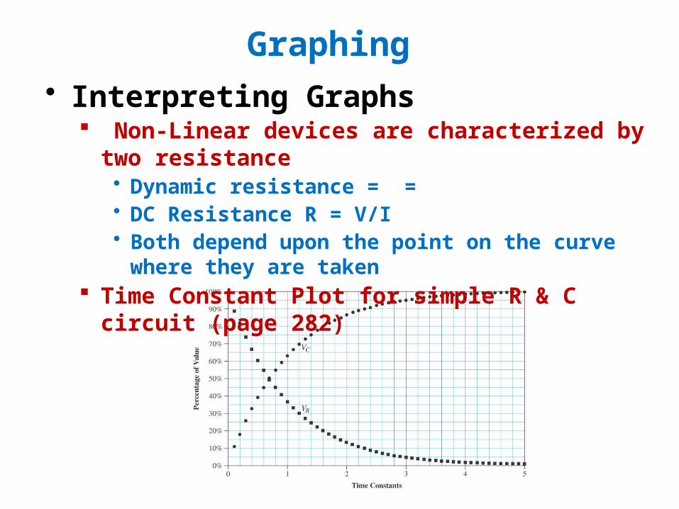
Non-Linear devices are characterized by two resistance• Dynamic resistance = = • DC Resistance R = V/I • Both depend upon the point on the curve where they are

taken Time Constant Plot for simple R & C circuit (page 282)

Graphing• Interpreting Graphs

Time Constant Plot for simple R & C circuit (page 282)• Do Example problems 13-4 and 13-5 on page 282• Practice Problems on page 13-5

• Plotting Curves Critical to determine the independent variable and the

dependent variable• For example in Fig 13-11 (page 280)

o Changes in V result in new values for Io Independent variable is usually plotted with respect to the

X Axiso The resulting dependent values are plotted with respect to

the y Axis

Graphing• Plotting Curves

Example Problem 13-6

Graphing• Plotting Curves

Example Problem 13-7