© Jeffrey S. Zax 2008 -14.1-

Chapter 14: Express yourself

8/24/08

Chapter 14: Express yourself -14.1-

Section 14.0: The Basics -14.1-

Section 14.1: Introduction -14.3-

Section 14.2: Dummy variables -14.3-

Section 14.3: Non-linear effects: The quadratic specification -14.8-

Section 14.4: Non-linear effects: Logarithms -14.18-

Section 14.5: Non-linear effects: Interactions -14.26-

Section 14.6: Conclusion -14.38-

Exercises -14.39-

Section 14.0: The Basics

For our purposes, regression has to be a linear function of the constant and coefficients so that their

estimators can be linear functions of the dependent variable. However, explanatory variables can appear

in discrete and non-linear form. These forms give us the opportunity to represent a wide and varied

range of possible relationships between the explanatory and dependent variables.

1. Section 14.2: Dummy variables identify the absence or presence of an indivisible

characteristic. The intercept for observations that don’t have this characteristic is a. The

effective intercept for observations that do have this characteristic is a+b2, where b2 is the slope

associated with the dummy variable. The slope b2 estimates the fixed difference in yi between

those that do and do not have the characteristic at issue.

© Jeffrey S. Zax 2008 -14.2-

2. Section 14.2: We fall into the dummy variable trap when we enter one dummy variable for a

particular characteristic, and another dummy variable for the opposite or absence of that

characteristic. These dummy variables are perfectly correlated, so slopes and their variances

are undefined. We only need one dummy variable, because its slope measures the difference

between the values of yi for observations that have the characteristic and those that don’t or

have its opposite.

3. Equations 14.13 and 14.18, Section 14.3: The quadratic specification is

y x xi i i i= + + +α β β ε1 22 .

$1xi is the linear term. $2xi2 is the quadratic term. If $1>0 and $2<0, small changes in xi increase

E(yi) when and reduce it when .xi < − ββ

1

22 xi > − ββ

1

22

4. Equations 14.35 and 14.36, Section 14.4: The semi-log specification is

ln .y xi i i= + +α β ε

The coefficient is the expected relative change in the dependent variable in response to an

absolute change in the explanatory variable.

β =

⎡

⎣⎢

⎤

⎦⎥E

yyx

i

Δ

Δ.

5. Equations 14.38 and 14.39, Section 14.4: The log-log specification is

ln ln .y xi i i= + +α β ε

© Jeffrey S. Zax 2008 -14.3-

The coefficient is the elasticity of the expected change in the dependent variable with respect

to the change in the explanatory variable:

β =

⎡⎣⎢

⎤⎦⎥

⎡⎣⎢

⎤⎦⎥

E yy

xx

i

i

Δ

Δ.

6. Equations 14.48 and 14.52, Section 14.5: Interactions allow the effect of one variable to

depend on the value of another. The population relationship with an interaction is

y x x x xi i i i i i= + + + +α β β β ε1 1 2 2 3 1 2 .

The change in the expected value of yi with a change in x1i

ΔΔ

yx

x i1

1 3 2= +β β .

Section 14.1: Introduction

The population relationship of Equation 12.1 is so flexible that it allows us to investigate a broad range

of relationships. We have already used it to help us understand the determinants of earnings, rent, Gross

National Income per capita and child mortality. However, it is capable of more. In our examples of the

last two chapters, all of the dependent and independent variables are continuous. Yet we may remember

some hints from Chapter 1 to the effect that interesting variables can come in other forms. This chapter

expands on those hints to explore some of the variety that is possible within the limits of Equation 12.1

Section 14.2: Dummy variables

In the regression of Figure 1.1, we include one variable indicating sex and five indicating racial or

© Jeffrey S. Zax 2008 -14.4-

ethnic identity. It’s easy to see why. Regardless of our exposure to current affairs, we have to be aware

that there is lots of concern as to whether these elements of identity have any effect on earnings. To

some degree, our sample validates this concern. It reveals large, significant negative effects for women

and blacks, and large, if imprecisely estimated effects, for several other racial and ethnic categories.

In Chapter 1 we identify the variables indicating sex, racial and ethnic identity as discrete, or

categorical. In fact, they are perhaps most commonly referred to as dummy variables. We don’t

mention this in chapter 1 because we are trying to get engaged with the material and it isn’t a good

place to get distracted by some nomenclature which seems a little pejorative and arbitrary. However,

we do demonstrate how incredibly useful they can be. More than half of the explanatory variables in

Figure 1.1 are dummies.

We also don’t say anything in chapter 1 about what, mathematically, a dummy variable is,

except to contrast them with continuous variables. This gives us a hint. As we say in chapter 1,

continuous random variables “take on a wide range of values”. This is easy to accept, since it clearly

describes our examples, earnings and age.

We haven’t thought about it much, but this wouldn’t ordinarily describe the kinds of

characteristics that we represent with dummy variables. For example, is it meaningful to talk about

being “more” or “less” of a Native Hawaiian or other Pacific Islander? More or less of a woman or a

man? In some contexts, as suggested by the obscure reference in footnote 10 of chapter 1, this may be

an interesting line of inquiry. Usually not. For most purposes, one either has the specified identity or

doesn’t.

This implies that discrete variables take on a limited range of values. In fact, it suggests that

only two might be necessary, one to indicate the presence of a characteristic and one to indicate its

absence. This is exactly how dummy variables work. They accomplish their purpose with only two

values, zero and one. We assign a value of one to an observation if it has the characteristic which is

represented by the dummy variable. We assign a value of zero if it doesn’t.

What does this look like? Return to the population relationship of Equation 12.1. Let’s assume

© Jeffrey S. Zax 2008 -14.5-

that the second explanatory variable, x2i, is categorical. Observations that do not have the characteristic

represented by x2i get the value of zero. For them, Equation 12.1 becomes

( )y xx

i i i

i i

= + + += + +α β β εα β ε

1 1 2

1 1

0.

(14.1)

In other words, these observations are really described by the population relationship of Equation 5.1,

with " as the constant and $1 as the coefficient.

For observations that have the characteristic represented by the categorical variable, x2i=1. This

means that Equation 12.1 becomes

( )

( )y x

xi i i

i i

= + + +

= + + +

α β β ε

α β β ε1 1 2

2 1 1

1

.(14.2)

Equation 14.2 implies that when the continuous variable x1i=0, observations with the indicated

characteristic have

yi = +α β2 (14.3)

In other words, for practical purposes, the constant for these observations is "+$2 rather than ", itself.

The effect of the characteristic represented by x2i is the difference between the expected value

of yi for those that have the characteristic and those that don’t. We can represent the former as

( )E y xi i| .2 1= (14.4)

This expression employs some notation that we saw in our statistics course, and reintroduce in footnote

20 of Chapter 6. To refresh our memories, the vertical strike “|” is read as “conditional on”, or, more

simply, “when”. We can read the expression in Equation 14.4 as representing “the expected value of

yi when x2i is equal to one”.

When x2i=1, the term in the parentheses of Equation 14.4 is given by Equation 14.2. Making

© Jeffrey S. Zax 2008 -14.6-

that substitution, we have

( ) ( )( )E y x E xi i i i| .2 2 1 11= = + + +α β β ε (14.5)

Assuming, once again, that ,i has the properties of chapter 5, Exercise 14.1 demonstrates that

( ) ( )E y x xi i i| .2 2 1 11= = + +α β β (14.6)

Continuing with the notation of Equation 14.4, the expected value of yi for observations lacking

the characteristic represented by x2i is

( )E y xi i| .2 0= (14.7)

Exercise 14.1 also helps us verify that the expected value of yi for these observations is

( )E y x xi i i| .2 1 10= = +α β (14.8)

Combining Equations 14.6 and 14.8, the effect of the characteristic represented by x2i is

( ) ( ) ( )( ) ( )E y x E y x x xi i i i i i| |

.2 2 2 1 1 1 1

2

1 0= − = = + + − +

=

α β β α β

β(14.9)

Equation 14.9 demonstrates that when x2i is a dummy variable, the population relationship of

equation 12.1 implies that the value of yi for an observation with the characteristic that it represents

differs from the value of yi for an observation without that characteristic, but with the same value of

x1i, by the fixed amount $2. Effectively, the constant for this latter observation is ". However, the

constant for the former observation is, as given in Equation 14.3, "+ $2.

This analysis carries over directly into the sample relationship. If x2i is the dummy variable,

then, when x1i=0, a in Equation 12.12 estimates the value of yi for observations that do not have the

characteristic indicated by x2i. The estimate of this value for observations that do have the characteristic

is a+b2. The difference between the values of yi for these two observations is b2. More generally, this

1 We prove this in Exercise 14.2.

© Jeffrey S. Zax 2008 -14.7-

is the difference between the values of yi for any two observations that differ in the characteristic

indicated by x2i, but that share the same value of x1i. This is exactly how we interpret the slopes for the

dummy variables in Figure 1.1.

Apart from interpretation, everything that we have said about the slopes from equation 12.12

is true for the slopes attached to dummy variables, so long as equation 12.1 is the true population

relationship and the properties of the ,is are as in chapter 5. In particular, the slope for a dummy

variable is the BLU estimator of $2. This may seem surprising, since dummy variables seem so

different in character from the continuous variables that have been our examples all along. It’s not

really, though. None of the results in Chapters 12 or 13 depend on the specific values that are valid for

x2i. As long as these values vary across observations, all of our formulas work regardless.

However, the specific values that are assigned to dummy variables heighten one of the dangers

that we discussed earlier. Imagine that x2i is a dummy variable representing women. We might think

that its slope estimates the distinct effect that women experience on their values of yi. From this

perspective, isn’t it possible that men also experience a distinct effect on their values of yi? Doesn’t this

suggest that men ought to have their own dummy variable, too?

This reasoning is superficially appealing, but wrong. Here’s why. If x2i identifies women, then

x2i=1 for each woman and x2i=0 for each man. If we simultaneously define x1i as a dummy variable that

identifies men, then x1i=1 for each man and x1i=0 for each woman. This means that, for all men, x1i=1

and x2i=0. For all women, x1i=0 and x2i=1. In other words, for men and women both,

x xi i1 21= − . (14.10)

There is a fixed relationship between x1i and x2i that holds throughout the sample! This means

that |CORR(x1i,x2i)|=1.1 All of the bad things that happen when this is true, which we examine in

Section 13.3 and Exercise 13.4, are ours to suffer if we enter a dummy variable for women and a

dummy variable for men in the same regression.

© Jeffrey S. Zax 2008 -14.8-

As we’ve just said, these bad things are not unique to dummy variables. They occur whenever

we put two explanatory variables that are perfectly correlated into the same regression. It’s just that

we’re especially likely to succumb to the temptation to do so when we work through an argument like

the one above. There, we almost convinced ourselves that if women deserved their own dummy

variable, so did men! This mistake is so common that it has its own name. It’s called the dummy

variable trap.

If we fall into it, it’s because we didn’t believe Equation 14.9. The message of that Equation

is clear: $2 measures only the difference between the effects of having and not having the characteristic

indicated by x2i. Exercise 14.1 demonstrates that this is true, regardless of whether the population

relationship includes the dummy variable for the characteristic, or the mirror-image dummy variable

for its absence.

Since there is only one difference, we only need one coefficient to represent it, and one slope

to estimate it. We get in trouble if we mistake $2 as the absolute effect of having the characteristic.

That’s when we begin to mislead ourselves into believing that it might make sense to measure the

absolute effect of not having the characteristic, as well.

Section 14.3: Non-linear effects: The quadratic specification

The word “linear” has appeared many times in this text. It always represents something that we like.

There are two interrelated types of linearity that are very important to us. First, it is important that yi

be a linear function of the parameters in the population relationship, apart from F. Second, it is

important that our estimators be linear functions of yi. These forms of linearity are valuable because,

with both, it’s easy, or at least relatively easy, to establish the basic properties of our estimators. If we

had to do without one or the other, we couldn’t derive expected values or variances for our slopes

without much more sophisticated tools.

However, this doesn’t mean that “nonlinear” is always bad. In particular, our population

relationships of equations 5.1 and 12.1 have adopted, implicitly, another form of linearity that is not

© Jeffrey S. Zax 2008 -14.9-

essential. This is linearity in the explanatory variables. In each of these equations, the explanatory

variables appear in additive terms. Each of these terms contains only one of the explanatory variables.

Within each term, the explanatory variable is raised to the first power and multiplied only by a constant.

Linearity in the explanatory variables is what gives us the first interpretation of Section 4.5.

There we explain that the slope of the regression represents the change that would occur in the

dependent variable if the explanatory variable changed by one unit. We’ve kept that interpretation in

mind ever since, right up until the last section. There, for the first time, it doesn’t quite fit. It isn’t

usually meaningful to talk about changing one’s sex, racial or ethnic identity by “one unit”. For this

reason, we have developed a new interpretation, which culminates in equation 14.9.

There’s another aspect of the interpretation in section 4.5 that we might want to vary

occasionally. There, b represents the estimated effect of a one-unit change in xi on yi, regardless of how

much xi we already have. The discussion in that section demonstrates that:

byx

=ΔΔ

.

The value of b depends only on the changes in xi and yi, not on their levels.

This is simply an analogy to the interpretation that is embedded in our population relationship.

To demonstrate, let’s change x1i by )x in equation 12.5. Let’s represent the change in the expected

value of yi by )y. The new expected value of yi is then

( ) ( )E y y x x x x x xi i i i i+ = + + + = + + +Δ Δ Δα β β α β β β1 1 2 2 1 1 2 2 1 . (14.11)

If we subtract Equation 12.5 from Equation 14.11, we get the change in the expected value of yi as

Δ Δy x= β1 .

Rearranging,

ΔΔ

yx= β1. (14.12)

2 We’ve already seen the square of an explanatory variable in the auxiliary regressions for theWhite test of heteroskedasticity, equations 9.5 and 13.44. However, the reason for its inclusion in theseequations, which we discuss prior to equation 9.5, is different than the purpose here.

© Jeffrey S. Zax 2008 -14.10-

The explanatory variable x1i doesn’t appear in Equation 14.12. Therefore, the effect of a change in x1i

doesn’t depend on the level of x1i.

In some contexts, this could be a problem. For example, throughout most of our intermediate

microeconomics course, we either have heard or will hear about “diminishing returns to scale”. This

is the idea that, while more of most things is better than less, the value of having additional things gets

smaller as the number of things we already have gets bigger.

On the consumption side, this captures the experience that most of us have, which is that the

third milk shake of the day is somehow less satisfying than the first. On the production side, it

represents the sense that if we give someone a broom, that person can do a lot of sweeping. If we give

that person a second broom, the amount of additional sweeping that gets done is not very impressive.

In these contexts, the effect of more xi depends on how much xi we already have. This is a non-

linear effect. We can represent it in our regression because what this requires is non-linearity in the

explanatory variables, not in the estimates. There are several ways to achieve this.

Perhaps the most common, and certainly the most flexible, is the quadratic specification. In

this specification, xi and its square both appear as explanatory variables.2 The population relationship

is therefore

y x xi i i i= + + +α β β ε1 22 . (14.13)

The term $1xi is the linear term. The term $2xi2 is the quadratic term. The expected value of yi from

this specification is

( )E y x xi i i= + +α β β1 22 . (14.14)

If we change xi by )x, the new expected value is

3 Those of us who are comfortable with calculus will recognize this as a restatement of thederivative

dydx

xi

ii= +β β1 22 .

© Jeffrey S. Zax 2008 -14.11-

( ) ( ) ( )

( )E y y x x x x

x x x x x xi i

i i i

+ = + + + +

= + + + + +

Δ Δ Δ

Δ Δ Δ

α β β

α β β β β β1 2

2

1 1 22

2 222 ,

(14.15)

where )y represents the change in the expected value. Subtracting Equation 14.14 from Equation

14.15, we get

( )Δ Δ Δ Δy x x x xi= + +β β β1 2 222 . (14.16)

If )x is small, then ()x)2 will be very small. In fact, it’s so small that we can disregard it. As long as

we stick to small changes in xi, we can rewrite Equation 14.16 as

Δ Δ Δy x x xi≈ +β β1 22 .

Dividing both sides by )x, we obtain3

ΔΔ

yx

xi≈ +β β1 22 . (14.17)

When the population relationship is Equation 5.1, the effect of xi on E(yi) is Equation 14.12.

When the population relationship includes a quadratic term, as in Equation 14.13, the effect of xi on

E(yi) is in Equation 14.17. The difference between Equations 14.12 and 14.17 is the term 2$2 xi. The

first thing that we can see in this difference is that it includes xi. Therefore, we’ve achieved our

immediate goal of making the effect of this variable depend on its current level.

The nature of this dependency depends on the signs of $1 and $2. The most common pattern is

probably, as we suggested above, consistent with declining returns to scale. This occurs when $1>0 and

$2<0. In this case, according to Equation 14.17, an increase in xi always contributes the positive amount

4 Again, from the perspective of calculus, we have simply set the first derivative equal to zeroin order to find the extreme values. The second derivative is

d ydx

i

i

2

2 22= β .

If, as in the example in the text, $2<0, this second derivative is negative and the value for xi that setsthe first derivative equal to zero is a maximum.

© Jeffrey S. Zax 2008 -14.12-

$1 to E(yi). If xi is small, that contribution will be diminished slightly by $2xi, but E(yi) will still

increase, overall. As xi gets larger, $2xi will become more important and the increase in E(yi) will get

smaller.

If xi is large enough, the positive contribution of $1 to E(yi) will be overwhelmed by the

negative contribution of $2xi, and E(yi) will decline. At what value for xi does its effect on the E(yi) stop

increasing and begin decreasing? In other words, what is the value of xi such that, for lower values,

and for higher values, in equation 14.17? Obviously, at this value for xi, theΔΔ

yx > 0 Δ

Δy

x < 0

positive contribution of $1 to E(yi) will just cancel the negative contribution of $2xi. This means

that .ΔΔ

yx = 0

Imposing this condition on Equation 14.17, we have

0 21 2= ≈ +ΔΔ

yx

xiβ β .

This occurs when4

xi ≈− ββ

1

22. (14.18)

Equation 14.18 says that when xi is less than , small increases in xi increase E(yi):− β

β1

22

5 In exercise 14.4 we confirm that these slopes are statistically significant.

© Jeffrey S. Zax 2008 -14.13-

. When xi is greater than , small increases in xi reduce E(yi): .ΔΔ

yx > 0

− ββ

1

22Δ

Δy

x > 0

We can demonstrate this in an example that first occurred to us in Section 1.7. There, we

discussed the possibility that workers accumulate valuable experience rapidly at the beginning of their

careers, but slowly, if at all, towards the end. In addition, at some point age reduces vigor to the point

where productivity declines, as well. This suggested that increasing age, serving as a proxy for

increasing work experience, should increase earnings quickly at early ages, but slowly at later ages and

perhaps negatively at the oldest ages.

We can test this proposition in the sample that we’ve been following since that Section. For

illustrative purposes, the regression with two explanatory variables that we develop in Chapters 12 and

13 is sufficient. Let’s set xi equal to age and xi2 equal to the square of age in the population relationship

of Equation 14.13. The sample analogue is then

y a b x b x ei i i i= + + +1 22 . (14.19)

Applied to our data, we obtain

( ) ( )( ) ( ) ( )

earnings age age squared error= − + − +50 795 3 798 40 68

14 629 748 6 9 044

, , . .

, . .(14.20)

As predicted, there are diminishing returns to age: b1=3,798>0 and b2=!40.68>0.5

Let’s figure out what all of this actually means. Equation 14.20 predicts, for example, that

earnings at age 20 would be $8,893. The linear term contributes $3,798×20=$75,960 to this prediction.

The quadratic term contributes !$40.68×(20)2=!$16,272. Lastly, the intercept contributes !$50,795.

Combined, they predict that the typical twenty-year old will earn somewhat less than $9,000 per year.

Similar calculations give predicted earnings at age 30 as $26,533, at 40 as $36,037, at 50 as $37,405

© Jeffrey S. Zax 2008 -14.14-

and at 60 as $30,637. These predictions confirm that typical earnings first goes up with age, and then

down.

Exercise 14.5 replicates the analysis of Equation 14.14 through 14.17 for the empirical

relationship of Equation 14.19. It proves that, in this context,

ΔΔ

yx

b b xi≈ +1 22 . (14.21)

where )y now represents the estimated change in the predicted value of yi. The value for xi at which

its effect on the predicted value of yi, reverses direction is $yi

xbbi =

− 1

22. (14.22)

Applying Equation 14.22 to the regression of Equation 14.20, maximum predicted earnings of $37,853

occur at about 46 and two-thirds years of age.

We might expect that there are diminishing returns to schooling, as well as to age. If for no

other reason, we observe that most people stop going to school at some point relatively early in their

lives. This suggests that the returns to this investment, as to most investments, must decline as the

amount invested increases.

We’re not quite ready to look at a regression with quadratic specifications in both age and

schooling, so let’s just rerun Equation 14.19 on the sample of Equation 14.20 with xi equal to years of

school and xi2 equal to the square of years of school. We get

( ) ( )( ) ( ) ( )

earnings yearsof school yearsof school squared error= − + +19 419 4 233 376 2

6 561 1110 49 37

, , . .

, , .(14.23)

This is a bit of a surprise. It’s still the case that b1 and b2 have opposite signs. However, b1<0 and b2>0.

Taken literally, this means that increases in years of schooling reduce earnings by b1, but

6 Formally, the second derivative in footnote 4 is now positive, because b2>0. This proves that,in this case, the solution to Equation 14.22 is a minimum.

© Jeffrey S. Zax 2008 -14.15-

increase them by b2xi. When years of school are very low, the first effect is larger than the second, and

additional years of schooling appear to actually reduce earnings. When years of school are larger, the

second effect outweighs the first, and additional years of schooling increase earnings.

There are two things about this that may be alarming. First, at least some years of schooling

appear to reduce productivity. Second, as years of schooling become larger, the increment to earnings

that comes from a small additional increase, b2xi, gets larger as well. In other words, the apparent

returns to investments in education are increasing! This raises an obvious question: If the next year of

education is even more valuable than the last one, why would anyone ever stop going to school?

Let’s use Equation 14.22 to see how worried we should be about the first issue. In a context

such as Equation 14.23, where b1<0 and b2>0, increases in xi first reduce, and then increase yi. This

means that Equation 14.22 identifies the value for xi that minimizes yi, rather than maximizes it as in

the example of equation 14.20.6 This value is 5.63 years of schooling. Additional schooling beyond

this level increases earnings.

This is a relief. Almost no one has less than six years of schooling, just 39 people out of the

1,000 in our sample.. Therefore, the implication that the first five or so years of schooling makes people

less productive is, essentially, an out-of-sample prediction. We speak about the risks of relying on them

in Section 7.5. Formally, they have large variances. Informally, there is often reason not to take them

too seriously.

Here, the best way to understand the predictions for these years is that they’re simply artifacts,

unimportant consequences of a procedure whose real purpose is elsewhere. Equation 14.23 is not trying

very hard to predict earnings for low levels of schooling, because those levels don’t actually appear in

the data. Instead, it’s trying to line itself up to fit the observed values in the sample, which almost all

start out at higher levels of schooling, to the quadratic form of Equation 14.19. Given this form, the best

way to do that happens to be to start from a very low value for earnings just below six years of

7 We reexamine the issues in this regression in Section 15.4.

© Jeffrey S. Zax 2008 -14.16-

schooling.

What about the implication that schooling has increasing returns? Based on Equation 14.21,

continuing in school for another year after completing the seventh grade increases predicted annual

earnings by $1,034. Continuing to the last year of high school after completing the eleventh year of

schooling increases predicted annual earnings by $3,291. Continuing from the fifteenth to the sixteenth

year of school, typically the last year in college, increases predicted annual earnings by $7,053. Taking

the second year of graduate school, perhaps finishing a master’s degree, increases predicted annual

earnings by $8,558. This is a pretty clear pattern of increasing returns. At the same time, it isn’t

shocking. In fact, these predictions seem pretty reasonable.

This still leaves the question of why we all stop investing in education at some point. Part of

the reason is that each additional year of school reduces the number of subsequent years in which we

can receive increased earnings by roughly one. So the lifetime return to years of schooling does not go

up nearly as quickly as the annual return. At some point, the lifetime return actually has to go down

because there aren’t enough years left in the working life to make up the loss of another year of current

income. Coupled with the possibility that higher levels of education require higher tuition payments

and more work, most of us find that, at some point, we’re happy to turn our efforts to something else.7

According to Exercise 14.7, the regression of apartment rent on the number of rooms and the

square of the number of rooms in the apartment yields the same pattern of signs as in Equation 14.23.

However, Exercise 14.8 demonstrates that the regression of child mortality rates on linear and quadratic

terms for the proportion of the rural population with access to improved water yields b1<0 and b2<0.

Moreover, the regression of child mortality rates on linear and quadratic terms for the proportion of the

rural population with access to improved water, discussed in Exercise 14.9, yields b1>0 and b2>0. How

are we to understand the quadratic specification of Equation 14.13 when both slopes have the same

sign?

In many circumstances, xi must be positive. This is certainly true in our principal example,

© Jeffrey S. Zax 2008 -14.17-

where the explanatory variable is education. It also happens to apply to our other examples. Age, the

number of rooms in an apartment and the proportion of rural residents with access to improved drinking

water have to be non-negative, as a matter of physical reality. The Corruption Perceptions Index is

defined so as to have only values between zero and ten.

In cases such as these, if b1 and b2 have the same signs, the two terms b1 and b2xi in Equation

14.21 also have the same signs. They reinforce each other. A small change in xi changes yi in the same

direction for all valid values of xi. As these values get larger, the impact of a small change in xi on yi

gets bigger.

In order for the effects of xi on yi to vary in direction, depending on the magnitude of xi, the two

terms to the right of the approximation in Equation 14.21 must differ in sign. This is still possible if b1

and b2 have the same sign, but only if xi can be negative. Another way to make the same point is to

realize that, if b1 and b2 have the same sign, the value of xi given by Equation 14.22 must be negative.

If the slopes are both positive, yi is minimized at this value for xi. If they are both negative, this value

for xi corresponds to the maximum for yi.

Regardless of the signs on b1 and b2, the second term in Equation 14.21 obviously becomes

relatively more important as the value of xi increases. We’ve already seen this when the slopes have

different signs, in our analyses of Equations 14.20 and 14.23. It will appear again in this context in

Exercise 14.7. Moreover, Exercises 14.8 and 14.9 will demonstrate that it’s also true when the slopes

have the same sign.

This illustrates an important point. If xi is big enough, the quadratic term in equation 14.19

dominates the regression predictions. The linear term becomes unimportant, regardless of the signs on

b1 and b2. Consequently, the quadratic specification always implies the possibility that the effect of xi

on yi will accelerate at high enough values of xi.

As we’ve already said, this looks like increasing returns to scale when b2>0, which we don’t

expect to see very often. Even if b2<0, the uncomfortable implication is still that, at some point, xi will

be so big that further increases will cause yi to implode. The question of whether or not we need to take

these implications seriously depends on how big xi has to be before predicted values of yi start to get

© Jeffrey S. Zax 2008 -14.18-

really crazy. If these values are rare, then these implications are, again, mostly out-of-sample

possibilities that don’t have much claim on our attention. If these values are not uncommon, as in the

example of earnings at high levels of education, then we have to give some careful thought as to

whether this apparent behavior makes sense.

Section 14.4: Non-linear effects: Logarithms

Another way to introduce non-linearity into the relationship between yi and its explanatory variables

is to represent one or more of them as logarithms. As we recall, the logarithm of a number is the

exponent that, when applied to the base of the logarithm, yields that number:

number base= logarithm .

What makes logarithms interesting, at this point, is that they don’t increase at the same rate as do the

numbers with which they are associated. They increase much less quickly.

For example, imagine that our base is 10. In this case, 100 can be expressed as 102. Therefore,

its logarithm is two. Similarly, 10,000 is 104. Consequently, its logarithm is four. While our numbers

differ by a factor of 100, the corresponding logarithms differ by only a factor of two. If we double the

logarithm again, to eight, the associated number increases by a factor of 10,000 to 108, or 100,000,000.

If we wanted the number whose logarithm was 100 times the logarithm of 100, we would have to

multiply 100 by 10198 to obtain 10 followed by 199 zeros.

Imagine that we specify our population relationship as

y xi i i= + +α β εlog . (14.24)

Equation 14.24 is a standard representation, but it embodies a couple of ambiguities. First, the

expression “log xi” means “find the value that, when applied as an exponent to our base, yields the

value xi”. In other words, this notation tells us to do something to xi. The expression “log” is, therefore,

a function, as we discussed in section 3.2. The expression “xi” represents the argument.

If we wanted to be absolutely clear, we would write “log(xi)”. We’ll actually do this in the text,

© Jeffrey S. Zax 2008 -14.19-

to help us keep track of what we’re talking about. However, we have to remember that it probably

won’t be done anywhere else. Therefore, we’ll adopt the ordinary usage in our formal equations.

Second, it should now be clear, if it wasn’t before, that $ does not multiply “l” or “lo” or “log”.

It multiplies the value that comes out of the function log (xi). If we wanted to be clearer still, we might

write the second term to the right of the equality in Equation 14.24 as $[log (xi)]. Conventionally,

however, we don’t. So we have to be alert to all of the implied parentheses in order to ensure that we

understand what is meant.

Notational curiosities aside, what does Equation 14.24 say about the relationship between xi and

yi? The first thing that it says is that a given change in log(xi) has the same effect on yi, regardless of

the value for xi. A one-unit change in log(xi) alters yi by $, no matter what.

This is of only marginal interest, because the logarithmic transformation of xi is just something

that we do for analytical convenience. The variable that we observe is xi. That’s also the value that is

relevant to the individuals or entities who comprise our sample. Therefore, we don’t care much about

the effect of log(xi) on yi. We’re much more interested in what Equation 14.24 implies about the effects

of xi, itself, on yi.

This implication is that a larger change in xi is necessary at high values of xi than at low values

of xi in order to yield the same change in yi. As we see just before Equation 14.24, a given change in

log(xi) requires larger increments at larger values for xi than at smaller values. As a given change in

log(xi) causes the same change in yi regardless of the value of xi, a given change in yi also requires

larger increments of xi at larger values for xi than at smaller values. In other words, the relationship

between xi and yi in Equation 14.24 is nonlinear.

If this was all that there was to the logarithmic transformation, we wouldn’t be very interested

in it. To its credit, it creates a non-linear relationship between xi and yi with only one parameter, so it

saves a degree of freedom in comparison to the quadratic specification of the previous section.

However, we lose a lot of flexibility. As we saw above, the effect of xi on yi can change direction in

the quadratic specification. The logarithmic specification forces a single direction on this relationship,

given by the sign of $. Moreover, it isn’t even defined when xi is zero or negative.

8 In this sense, e is just like B, another universal symbol for another irrational number,approximately equal to 3.14159.

© Jeffrey S. Zax 2008 -14.20-

Of course, the reason we have a whole section devoted to the logarithmic transformation is that

there is something more to it. However, in order to achieve it, we have to be very careful about the base

that we choose. Ten is a convenient base for an introductory example because it’s so familiar. However,

it’s not the one that we typically use.

Instead, we usually turn to the constant e. Note that we have now begun to run out of Latin as

well as Greek letters. This does not represent a regression error. Instead, it is the symbol that is

universally used to represent the irrational number whose value is approximately 2.71828.8 Logarithms

with this base are universally represented by the expression “ln”, generally read as “natural logarithm”.

What makes logarithms with e as their base so special? For our purposes, it’s this. Imagine that

we add a small increment to xi. We can rewrite this as

x x xx

xi ii

+ = +⎛⎝⎜

⎞⎠⎟Δ

Δ1 .

The natural logarithm of xi+)x is

( )ln ln .x x xx

xi ii

+ = +⎛⎝⎜

⎞⎠⎟

⎛

⎝⎜

⎞

⎠⎟Δ

Δ1

Using the rules of logarithms, we can rewrite this as

( )ln ln ln .xx

xx

xxi

ii

i1 1+⎛⎝⎜

⎞⎠⎟

⎛

⎝⎜

⎞

⎠⎟ = + +

⎛⎝⎜

⎞⎠⎟

Δ Δ (14.25)

The last term of Equation 14.25 is where the action is. When the base is e and )x is small,

9 At larger values for )x, the approximation gets terrible. For example, ln(e)=1. But theapproximation would give ln(e)=ln(2.71828)=ln(1+1.71828).1.71828. This is an error of more than70%!

© Jeffrey S. Zax 2008 -14.21-

ln .1+⎛⎝⎜

⎞⎠⎟ ≈

Δ Δxx

xxi i

(14.26)

In other words, the natural logarithm of 1+)x/xi is approximately equal to the percentage change in

xi represented by )x.

How good is this approximation? Well, when )x/xi=.01, ln(1.01)=.00995. So that’s pretty close.

When )x/xi=.1, ln(1.1)=.0953, which is only a little less accurate. However, the approximation is less

satisfactory when )x/xi=.2, because ln(1.2)=.182.9 In general, then, it seems safe to say that the

approximation in Equation 14.26 is valid for changes of up to about 10% in the underlying value.

The importance of this Equation 14.26 is easy to demonstrate. Rewrite Equation 14.24 in terms

of the natural logarithm of xi:

y xi i i= + +α β εln . (14.27)

With this specification, the expected value of yi is

( )E y xi i= +α β ln . (14.28)

Now make a small change in xi (10% or less) and write the new value of E(yi) as

( ) ( )E y y x xi i+ = + +Δ Δα β ln . (14.29)

With Equation 14.26, Equation 14.25 can be approximated as

( ) ( )ln ln .x x xx

xi ii

+ ≈ +ΔΔ

(14.30)

If we substitute Equation 14.30 into Equation 14.29, we get

© Jeffrey S. Zax 2008 -14.22-

( )E y y xx

xi ii

+ ≈ + +ΔΔ

α β βln , (14.31)

where )y again represents the change in the expected value. Now, if we subtract Equation 14.28 from

Equation 14.31 the result is

ΔΔ

yx

xi≈ β . (14.32)

Finally, we rearrange Equation 14.32 to obtain

β ≈⎛⎝⎜

⎞⎠⎟

Δ

Δ

yx

xi

. (14.33)

The numerator of Equation 14.33 is the magnitude of the change in the expected value of yi. The

denominator is, as we said above, the percentage change in xi. Therefore, $ in Equation 14.27

represents the absolute change in the expected value of yi that arises as a consequence of a given

relative change in xi.

The specification of Equation 14.27 may be appealing when, for example, the explanatory

variable does not have natural units. In this case, the interpretation associated with Equation 14.12 may

not be very attractive. How are we to understand the importance of the change that occurs in yi as a

consequence of a one-unit change in xi, if we don’t understand what a one-unit change in xi really

consists of?

This is obviously not a problem in our main example, where xi is years of schooling. We all

have a pretty good understanding of what a year of schooling is. Similarly, we know what it means to

count the rooms in apartment, so it’s easy to understand the change in rent that occurs when we add

one.

In contrast, the Corruption Perceptions Index, which we last saw in Exercise 14.9, is an

© Jeffrey S. Zax 2008 -14.23-

example. As we said in the previous section, this Index is defined so as to have values ranging from

zero to ten. However, these values convey only ordinal information: countries with higher values are

less corrupt than countries with lower values. They do not convey cardinal information: A particular

score or the magnitude of the difference between two scores are not associated, at least in our minds,

with a particular, concrete set of actions or conditions.

In other words, the units for the Corruptions Perceptions Index are arbitrary. An increase of one

unit in this Index doesn’t correspond to any additional actions or conditions that we could measure in

a generally recognized way. The Index could just as easily have been defined to vary from zero to one,

from zero to 100 or from eight to thirteen.

In sum, the absolute level of the Corruption Perceptions Index doesn’t seem to tell us much.

Consequently, we may not be too interested in the changes in Gross National Income associated with

changes in these levels. It might be informative to consider the effects of relative changes.

For this purpose, the sample regression that corresponds to the population relationship of

Equation 14.27 is

y a b x ei i i= + +ln .

If we apply this specification to our data on Gross National Income and the Corruption Perceptions

Index, we get the regression

( )( ) ( )

Gross National Income per capita

Corruption Perceptions Index ei

=

− + +13 421 17 257

2 183 1 494

, , ln .

, ,

(14.34)

The slope is significant at much better than 5%. It says that a 10% increase in the Corruption

Perceptions Index increases Gross National Income per capita by $1,726.

In practice, the specification of Equation 14.27 isn’t very common because we don’t often have

situations in which we expect a relative change in an explanatory variable to cause an absolute change

10 This was introduced in the pioneering work of Jacob Mincer, summarized briefly in Card(1999).

© Jeffrey S. Zax 2008 -14.24-

in the dependent variable. However, the converse situation, where an absolute change in an explanatory

variable causes a relative change in the dependent variable, occurs frequently. This is represented by

the population relationship

ln .y xi i i= + +α β ε (14.35)

Equation 14.35 is an example of the semi-log specification. Exercise 14.10 demonstrates that,

in this specification,

β =

⎡⎣⎢

⎤⎦⎥

E yy

xi

Δ

Δ.

(14.36)

The coefficient represents the expected relative change in the dependent variable, as a consequence of

a given absolute change in the explanatory variable.

The most famous example of the semi-log specification is almost surely the “Mincerian” human

capital earnings function.10 This specifies that the natural logarithm of earnings, rather than earnings

itself, is what schooling affects. According to the interpretation in Equation 14.36, the coefficient for

earnings therefore represents the percentage increase in earnings caused by an additional year of

schooling, or the rate of return on the schooling investment.

Once again, we return to our sample of Section 1.7 to see what this looks like. The sample

regression that corresponds to the population relationship in Equation 14.35 is

ln .y a bx ei i i= + +

With yi defined as earnings and xi as years of school, the result is

( ) ( )( )( )

ln . . .

. .

earnings yearsof school error= + +8 764 1055

1305 00985(14.37)

11 The sample for this regression contains only the 788 observations with positive earnings. The212 individuals with zero earnings must be dropped because the natural logarithm of zero is undefined.Perhaps surprisingly, this estimate is within the range produced by the much more sophisticated studiesreviewed by Card (1999). Exercise 14.11 gives us an opportunity to interpret another semi-logspecification.

12 Footnote 6 of chapter 13 declares that the ratio of a marginal change to an average is also anelasticity. Here’s why both claims are true:

[ ]elasticitychange

averagechange

yx

yx

yy

xx

relativechangein yrelativechangein x

= =

⎡⎣⎢

⎤⎦⎥

⎡⎣⎢

⎤⎦⎥

=

⎡⎣⎢

⎤⎦⎥ =

marginalΔ

ΔΔ

Δ.

© Jeffrey S. Zax 2008 -14.25-

Equation 14.37 estimates that each year of schooling increases earnings by approximately 10.6%.11

The last variation on the logarithmic transformation is the case where we believe that relative

changes in the dependent variable arise from relative changes in the explanatory variable. This is

represented by the population relationship

ln ln .y xi i i= + +α β ε (14.38)

The relationship in Equation 14.38 portrays the log-log specification.

Exercise 14.12 demonstrates that, in this specification,

β η=

⎡⎣⎢

⎤⎦⎥

⎡⎣⎢

⎤⎦⎥

=E y

y

xx

i

i

yx

Δ

Δ. (14.39)

The coefficient represents the expected relative change in the dependent variable, as a consequence of

a given relative change in the explanatory variable. As we either have learned or will learn in

microeconomic theory, the ratio of two relative changes is an elasticity.12 Equation 14.39 presents a

common, though not universal, notation for elasticities: the Greek letter 0, or “eta” (pronounced “ate-

uh”), with two subscripts indicating, first, the quantity being changed and, second, the quantity causing

the change.

13 Exercise 14.13 gives us another opportunity to interpret a regression of the form in Equation14.40.

14 We examine this particular specification in Exercise 14.17.

© Jeffrey S. Zax 2008 -14.26-

The log-log specification is popular because the interpretation of its coefficient as an elasticity

is frequently convenient. The sample analogue to the population relationship in Equation 14.38 is

ln ln .y a b x ei i i= + + (14.40)

Let’s revisit the relationship between child mortality and access to improved water from the regression

of Equation 12.43. If we respecify this regression in log-log form, the result is

( )

( ) ( )

ln . . ln%

.

. .

child mortalityof rural population with

access toimproved waterei= −

⎛⎝⎜

⎞⎠⎟ +9 761 1434

7216 1722(14.41)

The slope in Equation 14.41 is statistically significant at much better than 5%. It indicates that

an increase of one percent in the proportion of the rural population with access to improved drinking

water would reduce the rate of child mortality by almost one-and-a-half percent. This seems like a

pretty good return on a straightforward investment in hygiene.13

Section 14.5: Non-linear effects: Interactions

In our analysis of Equation 14.12, we observe that the effect of a change in x1i doesn’t depend on the

level of x1i. We might equally well observe that it doesn’t depend on the level of x2i, either. But why

should it? Well, we’ve already had an example of this in Table 1.4 of Exercise 1.4. There, we find

intriguing evidence that the effect of age on earnings depends on sex.14

Similarly, we might wonder if the effect of schooling depends on sex. The effects of age and

schooling might also vary with race or ethnicity. For that matter, the effects of age and school might

depend upon each other: If two people with the different ages have the same education, it’s likely that

© Jeffrey S. Zax 2008 -14.27-

the education of the older individual was completed at an earlier time. If the quality or content of

education has changed since then, the earlier education might have a different value, even if it is of the

same length.

The specification of Equation 12.1 doesn’t allow us to investigate these possibilities. Let’s

return to our principal example in order to see why. Once again, yi is annual earnings. The first

explanatory variable, x1i, is a dummy variable identifying women. The second, x2i, is a dummy variable

identifying blacks. For simplicity in illustration, we’ll ignore all of the other variables that earnings

might depend upon.

With the population relationship of Equation 12.1, we can distinguish between the expected

earnings of four different types of people. For men who are not black, x1i=0 and x2i=0. According to

Equation 12.5,

( ) ( ) ( )E y man not blacki | , .= + + =α β β α1 20 0 (14.42)

For women who are not black, x1i=1 and x2i=0. Therefore,

( ) ( ) ( )E y woman not blacki | , .= + + = +α β β α β1 2 11 0 (14.43)

For black men, x1i=0 and x2i=1. Consequently,

( ) ( ) ( )E y man blacki | , .= + + = +α β β α β1 2 20 1 (14.44)

Lastly, black women have x1i=1 and x2i=1:

( ) ( ) ( )E y woman blacki | , .= + + = + +α β β α β β1 2 1 21 1 (14.45)

In this specification, the expected value of earnings is constant for all individuals of a particular type.

However, the expected values of earnings for these four types of people are all different.

Still, this specification isn’t complete. The effects of being female and being black can’t

interact. The difference in expected earnings between a non-black woman and a non-black man, from

Equations 14.43 and 14.42, is

© Jeffrey S. Zax 2008 -14.28-

( ) ( ) ( )E y woman not black E y man not blacki i| , | , .− = + − =α β α β1 1(14.46)

The difference between a black woman and a black man, from Equations 14.45 and 14.44, is

( ) ( ) ( ) ( )E y woman black E y man blacki i| , | , .− = + + − + =α β β α β β1 2 2 1(14.47)

These differences are identical, even though the employment traditions of men and women might differ

across the two races. Exercise 14.14 demonstrates that, similarly, the specification of Equation 12.1

forces the effect of race to be the same for both sexes.

Another way to describe the implications of Equation 12.1 in this context is that the effects of

race and sex are additive. Expected earnings differ by a fixed amount for two individuals of the same

sex. They differ by another fixed amount for two individuals of the same race. The difference between

two individuals who differ in both sex and race is simply the sum of these two differences. Of course,

it’s possible that these effects really are additive. But why insist on it, before even looking at the

evidence?

In other words, we prefer to test whether additivity is really appropriate, rather than to assume

it. In order to do so, we need to introduce the possibility that the effects are not additive. This means

that we need to allow for the possibility that the effects of race and sex are interdependent. These kinds

of interdependencies are called interactions.

Interactions are another form of non-linear effect. The difference is that, instead of changing

the representation of a single explanatory variable, as we do in the previous two Sections, interactions

multiply two or more explanatory variables. What this means is that we create a new variable for each

observation, whose value is given by the product of the values of two other variables for that same

observation.

The simplest representation of an interaction in a population relationship is

y x x x xi i i i i i= + + + +α β β β ε1 1 2 2 3 1 2 . (14.48)

In this relationship, the expected value of yi is

15 Exercise 14.15 demonstrates that, similarly, the effect of a change in x2i in Equation 14.49depends on the level of x1i.

© Jeffrey S. Zax 2008 -14.29-

( )E y x x x xi i i i i= + + +α β β β1 1 2 2 3 1 2 . (14.49)

Following what is now a well-established routine, let’s change x1i by )x1 and see what happens.

Representing, yet again, the change in the expected value of yi as )y, Equation 14.49 gives us

( ) ( ) ( )E y y x x x x x xx x x x x x x

i i i i i

i i i i i

+ = + + + + +

= + + + + +

Δ Δ Δ

Δ Δ

α β β βα β β β β β

1 1 1 2 2 3 1 1 2

1 1 2 2 3 1 2 1 1 3 2 1.(14.50)

When we, predictably, subtract Equation 14.49 from Equation 14.50, we get

Δ Δ Δy x x xi= +β β1 1 3 2 1. (14.51)

Finally, we divide both sides of Equation 14.51 by )x1:

ΔΔ

yx

x i1

1 3 2= +β β . (14.52)

Equation 14.52 states that the effect of a change in x1i on the expected value of yi has a fixed

component, $1, and a component that depends on the level of x2i, $3x2i. This second term embodies the

interdependence.15

To see how this works in practice, let’s return to our example of Equations 14.42 through 14.47.

In this case, each of the individual variables, x1i and x2i, has only the values zero and one. This means

that their product, x1ix2i, can also have only these two values. It can only equal one if both of its

individual factors also equal one.

In other words, x1ix2i=1 only if x1i=1 and x2i=1. The first condition, x1i=1, identifies the

observation as a woman. The second condition, x2i=1, identifies the observation as a black. Therefore,

the value x1ix2i=1 identifies the observation as a black woman.

Consequently, Equation 14.49 gives expected earnings for men who are not black as

© Jeffrey S. Zax 2008 -14.30-

( ) ( ) ( ) ( )E y man not blacki | , .= + + + =α β β β α1 2 30 0 0 (14.53)

For women who are not black,

( ) ( ) ( ) ( )E y woman not blacki | , .= + + + = +α β β β α β1 2 3 11 0 0 (14.54)

For black men,

( ) ( ) ( ) ( )E y man blacki | , .= + + + = +α β β β α β1 2 3 20 1 0 (14.55)

Lastly, for black women,

( ) ( ) ( ) ( )E y woman blacki | , .= + + + = + + +α β β β α β β β1 2 3 1 2 31 1 1 (14.56)

With this specification, expected earnings for non-black men, non-black women and black men

in Equations 14.53 through 14.55 are the same as in Equations 14.42 through 14.44. In other words,

the specification of Equation 14.48 and that of Equation 12.1 have the same implications for these three

groups. Consequently, the difference in expected earnings between non-black women, given in

Equation 14.54, and non-black men from Equation 14.53 is simply $1. It’s identical to this difference

under the specification of Equation 12.1, given in Equation 14.46.

How does this compare to the difference that is given by Equation 14.52? That equation

requires some careful interpretation in our current context, because we usually think of terms beginning

with “)” as indicating small changes. Here, all of the explanatory variables are dummies. This means

that the only possible changes are from zero to one and back. In other words, here Equation 14.52 must

be comparing two different individuals, one with the characteristic indicated by x1i and one without.

In addition, it is helpful to recall that these two individuals must be of the same race. How do

we know that? Because we allow the terms $2x2i in Equations 14.49 and 14.50 to cancel when we

subtract the former from the latter to get Equation 14.51. This is only valid if both individuals have the

same value for x2i, which, here, means the same racial identity.

With these preliminaries, Equation 14.52 tells us that the difference between the expected

© Jeffrey S. Zax 2008 -14.31-

earnings for a woman and a man when x2i=0, that is, when both are non-black, should be exactly $1.

It agrees perfectly with the difference between Equations 14.53 and 14.54.

The difference between Equations 14.48 and 12.1 is in their implications for black women.

Expected earnings for black women in Equation 14.56 are again a constant. However, it differs from

the constant of Equation 14.45 by the coefficient on the interaction term, $3. Therefore, the difference

between expected earnings for a black woman and for a black man is, from Equations 14.56 and 14.55,

( ) ( ) ( ) ( )E y woman black E y man blacki i| , | , .− = + + + − + = +α β β β α β β β1 2 3 2 1 3(14.57)

This, again, is exactly the difference given by Equation 14.52, now that x2i=1. It is not the same

as the difference between expected earnings for a non-black woman and for a non-black man unless

$3=0. If $3…0, than the effects of sex and race on earnings are interdependent.

As always, we can check this out empirically with our sample of Section 1.7. The sample

counterpart to the population relationship of Equation 14.48 is

y a b x b x b x x ei i i i i i= + + + +1 1 2 2 3 1 2 . (14.58)

With x1i and x2i representing women and blacks, the estimates are

( ) ( ) ( )( ) ( ) ( ) ( )

earnings female black black female error= − − + +40 060 18 612 13163 11561

1 923 2 740 7 317 10 354

, , , , .

, , , ,(14.59)

The slopes for women and blacks are familiar. They are only slightly larger in magnitude than

in our very first regression of Figure 1.1. However, the slope for black women is positive and nearly

as large in magnitude as the slope for all blacks. For black women, the magnitude of the combined

effect of these two slopes is essentially zero. This suggests that, on net, earnings for black women are

not affected by race. The regression of Equation 14.59 estimates the expected value of earnings for

black women, as given in Equation 14.56, as approximately equal to that for non-black women in

Equation 14.54.

16 We build the foundation for this prediction in Exercise 7.12.

© Jeffrey S. Zax 2008 -14.32-

This conclusion must be drawn with some caution. The t-statistic of the slope for all blacks is

1.80, significant at better than 10%. However, the t-statistic of the slope for black women is only 1.12,

with a prob-value of .2644. This fails to reject the null hypothesis that there is no interaction between

race and sex, H0: $3=0.

At the same time, the regression of Equation 14.59 also fails to reject the joint null hypothesis

that the effects of being black and being a black woman cancel each other. This hypothesis is equivalent

to the null hypothesis that expected earnings for non-black and black women are the same. Formally,

it is H0: $2+$3=0. The F-statistic for the test of this hypothesis is only .05, with a prob-value of .8270.

In sum, the evidence from Equation 14.59 is weak. The sample upon which it is based does not

contain enough information to estimate the interaction effect of being a black female very precisely.

Consequently, this Equation can’t tell the difference, at least to a statistically satisfactory degree,

between the expected earnings of black women and black men, or between black women and non-black

women.

Fortunately, we have stronger evidence available to us. If we repeat the regression of Equation

14.59 using the entire sample of Section 7.6, the result is

( ) ( ) ( )( ) ( ) ( ) ( )

earnings female black black female error= − − + +40 784 19 581 14 520 14 352

1534 218 7 620 2 8701

, , , , .

. . . .(14.60)

The intercept and slopes of Equation 14.60 do not differ from those of Equation 14.59 in any important

way.

However, the sample for Equation 14.60 is more than 100 times as large as that for Equation

14.59. Predictably, the standard deviations here are less than one-tenth of those for the smaller sample.16

Exercise 14.16 confirms that Equation 14.60 rejects the null hypothesis that H0: $3=0 but again fails

to reject the null hypothesis H0: $2+$3=0. This evidence strongly suggests that expected earnings for

black and non-black women are similar. Race appears to affect expected earnings only for black men.

17 In Exercise 14.17 we demonstrate that it would be a mistake to add separate interaction termsfor observations with x1i=0 and x1i=1 in this specification.

18 We consider the reasons for this change in Exercise 14.18.

© Jeffrey S. Zax 2008 -14.33-

When x1i and x2i are both dummy variables, the interaction between them has the effect of

altering the “constant” for the case where x1i=1 and x2i=1, as we show in our discussion of Equation

14.57. When x2i is a continuous variable, the effect of the interaction term is to assign different slopes

to x2i, depending on whether x1i=0 or x1i=1. In the first case, Equation 14.49 again reduces to Equation

5.1:

( ) ( ) ( )E y x x xi i i i= + + + = +α β β β α β1 2 2 3 2 2 20 0 .

In the second case, Equation 14.49 reduces to a more elaborate version of Equation 5.1:

( ) ( ) ( ) ( ) ( )E y x x xi i i i= + + + = + + +α β β β α β β β1 2 2 3 2 1 2 3 21 1 .

$3 is the difference between the slopes for observations with x1i=0 and x1i=1.17

We can illustrate this in the sample of Equation 14.59 by redefining x2i as schooling. Equation

14.58 becomes

( ) ( )( ) ( ) ( )

( )( )

earnings female yearsof schooling

yearsof schooling for women error

= − + +

− +

21541 10 207 4 841

6 098 8 887 4661

2 226

682 0

, , ,

, , .

, .

.

(14.61)

This is quite provocative! The slope for the female dummy variable is now positive!18 However, it’s

also statistically insignificant. The best interpretation is therefore that there’s no evidence that the

constant component of earnings differs between men and women.

The reason that the slope for the female dummy variable has changed signs, relative to previous

© Jeffrey S. Zax 2008 -14.34-

regressions, is that the slope for women’s years of schooling is negative. Moreover, it’s statistically

significant at much better than 5%. This indicates that $3 is negative. In fact, the estimated return to

schooling for women is b2+b3=2,615, only slightly more than half the return to schooling for men!

While previous regressions have suggested that women’s earnings are less than men’s by a rather large

constant, Equation 14.61 indicates instead that the gap between them is relatively small at low levels

of education, but increases substantially with higher levels of schooling!

The third possible form of interaction is between two continuous variables. The interpretation

of this form is directly embodied in Equation 14.52. It specifies that the slope for each variable is

different, depending on the level of the other.

This is probably the most difficult interpretation to understand. Fortunately, we have the

illustration that we suggested at the beginning of the section. Individuals of different ages typically had

their educations at different times. Educations of different vintages may have different values, for many

reasons. The content of education has certainly changed. The quality may have changed as well. Of

course, these changes could either reduce or increase the value of older educations relative to those that

are more recent.

At the same time, the value of work experience may vary with education. Workers with little

education may not have the foundation necessary to learn more difficult work tasks. If so, they will

benefit less from experience than will workers who are better educated. This suggests that experience

and education may be complements. As we approximate experience here with the variable measuring

age, this suggests that the returns to age will increase with higher education.

Doesn’t this sound interesting? Let’s find out what the data can tell us. Returning, yet again,

to the sample of Equation 14.59, we retain the definition of x2i as schooling from Equation 14.61. We

and now define x1i as age. Here’s what we get:

© Jeffrey S. Zax 2008 -14.35-

Table 14.1

Predicted earnings from Equation 14.62

Years of Schooling

Age 8 12 16 1830 $17,815 $26,722 $35,630 $40,08440 $23,753 $35,630 $47,507 $53,44550 $29,692 $44,538 $59,384 $66,80760 $35,630 $53,445 $71,260 $80,168

( ) ( )( ) ( ) ( )

( )( )

earnings age yearsof schooling

age yearsof schooling error

= − +

+ +

7 678 552 5 582 2

17 270 402 0 1 366

74 23

3137

, . .

, . ,

. * .

.

(14.62)

This is really provocative! According to Equation 14.62, b1 and b2 are both statistically

insignificant! This suggests that $1=0 and $2=0: Neither age nor education has any reliable effect on

earnings, on their own. In contrast, b3 is significantly greater than zero. In sum, Equation 14.62

indicates that the only effect of schooling or age on earnings comes from the second term to the right

of the equality in Equation 14.52, $3x2i, for x1i, and its analogue from Exercise 14.15, $3x1i for x2i.

What, quantitatively, does this mean? The best way to illustrate this is with Table 14.1. This

table presents values of b3x1ix2i for selected values of x1i and x2i. These values are estimates of the

contribution of the interaction between age and schooling to earnings, $2x1ix2i.

Looking down each of the columns in Table 14.1, we see that increases in age make bigger

contributions to earnings at higher levels of education. Looking across each of the rows in Table 14.1,

© Jeffrey S. Zax 2008 -14.36-

we see that higher levels of education make bigger contributions to earnings at higher ages.

The estimates in Table 14.1 have some claim to be the best predictions of earnings that can be

made on the basis of Equation 14.62. First, they actually look pretty reasonable. A thirty-year old with

no high school makes $17,815 per year? A sixty-year old with a masters degree makes $80,168?

Nothing here conflicts substantially with our intuition.

More seriously, the values of a, b1 and b2 are statistically insignificant. They fail to reject the

individual hypotheses H0: "=0, H0: $1=0 and H0: $2=0. If we were to impose these null hypotheses on

the population relationship of Equation 14.49, it would become E(yi)=$3x1ix2i. In this case,

The values in Table 14.1 would be the appropriate predictions of expected earnings.$ .y b x xi i i= 3 1 2

The question of whether we are comfortable imposing these null hypotheses turns on two

points. First, how certain are we, based on intuition or formal economic reasoning, that education and

age should make independent contributions to earnings? Second, how confident are we that the data

upon which we base Equation 14.62 are adequate for the purpose of testing whether these contributions

exist?

In this case, we have pretty easy answers. It’s hard to accept that age or education don’t make

any impact on earnings at all, apart from their interaction. Moreover, using Equation 13.29, we find that

the test of the joint hypothesis H0: $1=$2=0 in Equation 14.62 yields an F-statistic of 11.02, with a

prob-value of less than .0001. This is a pretty powerful rejection. So even though this equation can’t

pin down the individual values of $1 and $2 very accurately, it’s almost certain that they’re not both

zero.

Also, however good is the sample of Equation 14.62, we know that we have a much larger

sample available. We’ve used it most recently to calculate Equation 14.60. Therefore, the right thing

to do is to reexamine the question asked by Equation 14.62 in this larger sample. The result is

19 Exercise 14.19 examines the magnitudes of these slopes.

© Jeffrey S. Zax 2008 -14.37-

( ) ( )( ) ( ) ( )

( )( )

earnings age yearsof schooling

age yearsof schooling error

= − − +

+ +

7 678 2011 2 079

1 232 28 64 98 60

39 99

2 259

, . ,

, . .

. * .

.

(14.63)

The signs on the slopes of Equation 14.63 are identical to those in 14.62.19 However, the

standard errors are all, as we would expect, much smaller. All three slopes are statistically significant

at much better than 5%. The estimates here of $1 and $2 indicate that both x1i and x2i make independent

contributions to earnings.

The estimate of $3 again indicates that age and schooling are complements. Returning to

Equation 14.52, we find that the total effect of a change in age on earnings is

( )( ) ( )Δ

Δ

earningsage

yearsof schooling= − +2011 39 99. . . (14.64)

Formally, Equation 14.64 implies that increases in age reduce earnings if years of schooling are five

or fewer. As we observe in our discussion of Equation 14.23, this is not particularly interesting because

almost everyone has more schooling than this.

Regardless, each additional year of schooling increases the annual return to age, and

presumably to experience, by approximately $40. For someone with an eighth-grade education, each

additional year of experience should increase earnings by almost $120. For someone with a college

degree, earnings should go up by nearly $440 with an additional year.

Similarly, the total effect of schooling on earnings is

20 We’ve already seen variables expressed as reciprocals in the WLS specification of Equation9.7. However, the reciprocal there addresses statistical rather than behavioral concerns.

© Jeffrey S. Zax 2008 -14.38-

( )( ) ( )Δ

Δ

earningsyearsof schooling

age= +2 079 39 99, . .

At age 20, an additional year of schooling increases earnings by $2,879. At age 40, the increase is

$3,679. At age 60, it is $4,478.

Section 14.6: Conclusion

We can see that dummy variables, quadratic and logarithmic specifications, and interaction terms allow

us to construct regression specifications that are much more flexible than might be apparent from

Equation 12.1 alone. Moreover, our discussion has by no means exhausted the possibilities. Nonlinear

relationships may occasionally be represented by variables expressed as reciprocals or even

trigonometric functions.20

We may, on rare occasions, find regression specifications that try to achieve even more

flexibility, and complexity, by appending a cubic or even a quartic term in the explanatory variable.

The first would contain the quantity xi3, the second the quantity xi

4. With a cubic term, the relationship

between xi and yi can change directions twice. With a quartic term, it can happen three times. If these

patterns are appropriate for the behavior under study, these specifications can be very revealing. If not,

of course, they can be thoroughly confusing.

The overall message of this chapter is that we don’t always have to force the relationship in

which we’re interested to fit the simple specification of Equation 12.1. We will need much more

training before we can explore nonlinear relationships among the parameters. But with a little

ingenuity, nonlinear treatments of the variables can modify Equation 12.1 to accommodate a much

broader range of behavior than we might have otherwise guessed.

© Jeffrey S. Zax 2008 -14.39-

Exercises

14.1 Assume that ,i has the properties of chapter 5.

a. Apply the rules of expectations from chapter 5 to Equation 14.5 in order to derive

Equation 14.6.

b. Replace Equation 14.1 in Equation 14.7 and repeat the analysis of a. to derive Equation

14.8.

c. Redefine x2i as equal to one when the characteristic in question is not present, and zero

when it is. Restate Equations 14.1 through 14.9 with this definition. How do these

restated equations differ from the originals? What, now, is the difference in E(yi) for

observations with and without the characteristic? How does this compare to the

difference in Equation 14.9?

14.2 Section 14.2 alludes to two circumstances in which the regression calculations are not well-

defined.

a. Towards the end of section 14.2, we make the claim that the results pertaining to

regression slopes in Chapters 12 and 13 don’t depend on the values of the associated

explanatory variables, “(a)s long as these values vary across observations”. Why did

we have to add this qualification? What happens if the value of an explanatory variable

does not vary across observations?

b. Demonstrate that the sample CORR(x1i,x2i)=!1 if equation 14.10 is true. Recall the

consequences from chapter 13.

14.3 Imagine that we intend x2i to be a dummy variable in the population relationship of equation

12.1.

a. Unfortunately, we make a mistake. We assign the value x2i=2 to observations that have

the characteristic of interest, and the value x2i=1 to observations that do not. Modify the

© Jeffrey S. Zax 2008 -14.40-

analysis of Equations 14.1 through 14.9 to derive the appropriate interpretation of $2

in this case.

b. Based on the answer to a., what would be the consequence if we assign the value x2i=3

to observations that have the characteristic of interest, and the value x2i=2 to

observations that do not? What about the values 5 and 4? What about any two values

that differ only by one?

c. Based on the answers to a. and b., what would be the consequence if we assign the

value x2i=3 to observations that have the characteristic of interest, and the value x2i=1

to observations that do not? What about any two values that differ by two? What about

any two values that differ by any amount?

14.4 Consider the regression in equation 14.20.

a. Demonstrate, either with confidence intervals or two-tailed hypothesis tests, that a, b1

and b2 are statistically significant.

b. Verify the predicted earnings at ages 30, 40, 50 and 60.

c. Use equation 14.22 to verify that maximum predicted earnings occur at approximately

46 and two-thirds years of age.

14.5 Return to the quadratic regression specification of equation 14.19. The predicted value of yi

from this specification is

$ .y a b x b xi i i i= + + 22

a. Change xi by )x. Demonstrate that the new predicted value is

( )$ .y y a b x b x b x b x x b xi i i i i i+ = + + + + +Δ Δ Δ Δ22

2 222

b. Subtract the expression for from the result of a. to obtain$yi

© Jeffrey S. Zax 2008 -14.41-

( )Δ Δ Δ Δy b x b x x b xi i= + +2 2 22 .

c. State the assumption that is necessary in order to approximate the relationship in b. with

Δ Δ Δy b x b x xi i≈ + 2 2 .

d. Starting with the answer to c., prove that

ΔΔ

yx

b b xi i≈ + 2 2 .

14.6 Consider the regression in equation 14.23.

a. Demonstrate, either with confidence intervals or two-tailed hypothesis tests, that a, b1

and b2 are statistically significant.

b. Verify the predicted changes in annual earnings at seven, 11, 15 and 17 years of

schooling.

c. Use equation 14.22 to verify that minimum predicted earnings occur at approximately

5.63 years of schooling.

14.7 The quadratic version of the regression in Equation 13.42 is

( ) ( )( )( ) ( )

rent all rooms all rooms ei= − + +668 4 4344 1570

49 91 26 97 3329

2. . . .

. . .

a. Interpret the signs and values of b1 and b2 following the analysis of section 14.3.

b. Check, either with confidence intervals or two-tailed hypothesis tests, whether b1 or b2

are statistically significant. Does the answer alter or confirm the interpretations of a.?

c. Predict rents for apartments of two, four, six and eight rooms. Compare these

predictions. Does the comparison seem plausible? If yes, why? If no, why not, and what

© Jeffrey S. Zax 2008 -14.42-

might explain the anomalies?

14.8 The regression of Equation 12.43, with standard errors, is

( ) ( )

child mortalityof rural population with

access toimproved waterei= −

⎛⎝⎜

⎞⎠⎟ +2005 1764

14 66 1973

. .%

.

. .

a. Demonstrate, either with confidence intervals or two-tailed hypothesis tests, that b is

statistically significant.

b. The quadratic specification of this regression yields

child mortalityof rural population with

access toimproved water

of rural population withaccess toimproved water

ei

= −⎛⎝⎜

⎞⎠⎟

−⎛⎝⎜

⎞⎠⎟ +

152 5 05644

013052

. .%

.%

.

Interpret the signs and values of b1 and b2 following the analysis of section 14.3.

c. For this regression, SD(b1)=1.125 and SD(b2)=.00846 . Are either of these slopes

statistically significant? Does the answer to this alter or confirm the interpretations of

b.?

d. The R2 value for this regression is .3865. Test the null hypothesis H0: $1=0 and $2=0

using equation 13.35. What can we conclude about the joint effects of the variable

measuring rural access to water and its square on child mortality? Comparing this

conclusion to that of c., what can we conclude about the relationship between these two

variables?

© Jeffrey S. Zax 2008 -14.43-

e. Use equation 13.36 to derive the correlation between b1 and b2.

f. Equation 12.43, with the linear explanatory variable replaced by the quadratic

explanatory variable, is

( ) ( )

child mortalityof rural population with

access toimproved waterei= −

⎛⎝⎜

⎞⎠⎟ +1508 01346

9 390 00147

2

. .%

.

.

Is b statistically significant?

g. Compare equation 12.43, the quadratic specification in b. and the bivariate regression

in f. In addition to what we’ve already learned about these regressions in this exercise,

their R2 values are, respectively, .3754, .3865 and .3864. Which regression seems to be

the most compelling way to represent the information in the sample? Why? Predict the

child mortality rates for water accessibility rates of 30%, 60% and 90% using each of

the regressions. Does it make much difference which regression we use? Why or why

not?

14.9 The regression of Equation 12.41, with standard errors, is

( )( ) ( )

Gross National Income per capita

Corruption Perceptions Index ei

=

− + +7 399 4 013

1 373 277 7

, , .

, .

a. Demonstrate, either with confidence intervals or two-tailed hypothesis tests, that b is

statistically significant.

b. The quadratic specification of this regression yields

© Jeffrey S. Zax 2008 -14.44-

( )( )

Gross National Income per capita

Corruption Perceptions Index

Corruption Perceptions Index ei

=

− +

+ +

1 618 1 403

23912

, ,

. .

Interpret the signs and values of b1 and b2 following the analysis of section 14.3.

c. For this regression, SD(b1)=1,398 and SD(b2)=125.6. Are either of these slopes

statistically significant? Does the answer to this alter or confirm the interpretations of

b.?

d. For this regression, SD(a)=3,323. Is the intercept statistically significant? At this point,

what do we think of this regression?

e. The R2 value for this regression is .7507. Test the null hypothesis H0: $1=0 and $2=0

using equation 13.35. What can we conclude about the joint effects of the Corruption

Perceptions Index and its square on child mortality? Comparing this conclusion to that

of c., what can we conclude about the relationship between these two variables?

Comparing this conclusion to that of d., what can we conclude about this regression as

a whole?

f. Use equation 13.36 to derive the correlation between b1 and b2.

g. Equation 12.41, with the linear explanatory variable replaced by the quadratic

explanatory variable, is

( )( ) ( )

Gross National Income per capita

Corruption Perceptions Index ei

=

+ +1 610 362 8

837 9 24 53

2, . .

. .

Is b statistically significant?

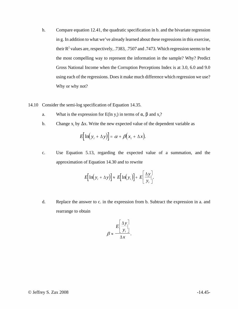
© Jeffrey S. Zax 2008 -14.45-

h. Compare equation 12.41, the quadratic specification in b. and the bivariate regression

in g. In addition to what we’ve already learned about these regressions in this exercise,

their R2 values are, respectively, .7383, .7507 and .7473. Which regression seems to be

the most compelling way to represent the information in the sample? Why? Predict

Gross National Income when the Corruption Perceptions Index is at 3.0, 6.0 and 9.0

using each of the regressions. Does it make much difference which regression we use?

Why or why not?

14.10 Consider the semi-log specification of Equation 14.35.

a. What is the expression for E(ln yi) in terms of ", $ and xi?

b. Change xi by )x. Write the new expected value of the dependent variable as

( )[ ] ( )E y y x xi iln .+ = + +Δ Δα β

c. Use Equation 5.13, regarding the expected value of a summation, and the

approximation of Equation 14.30 and to rewrite

( )[ ] ( )[ ]E y y E y Ey

yi ii

ln ln .+ ≈ +⎡

⎣⎢

⎤

⎦⎥Δ

Δ

d. Replace the answer to c. in the expression from b. Subtract the expression in a. and

rearrange to obtain

β ≈

⎡

⎣⎢

⎤

⎦⎥E

yyx

i

Δ

Δ.

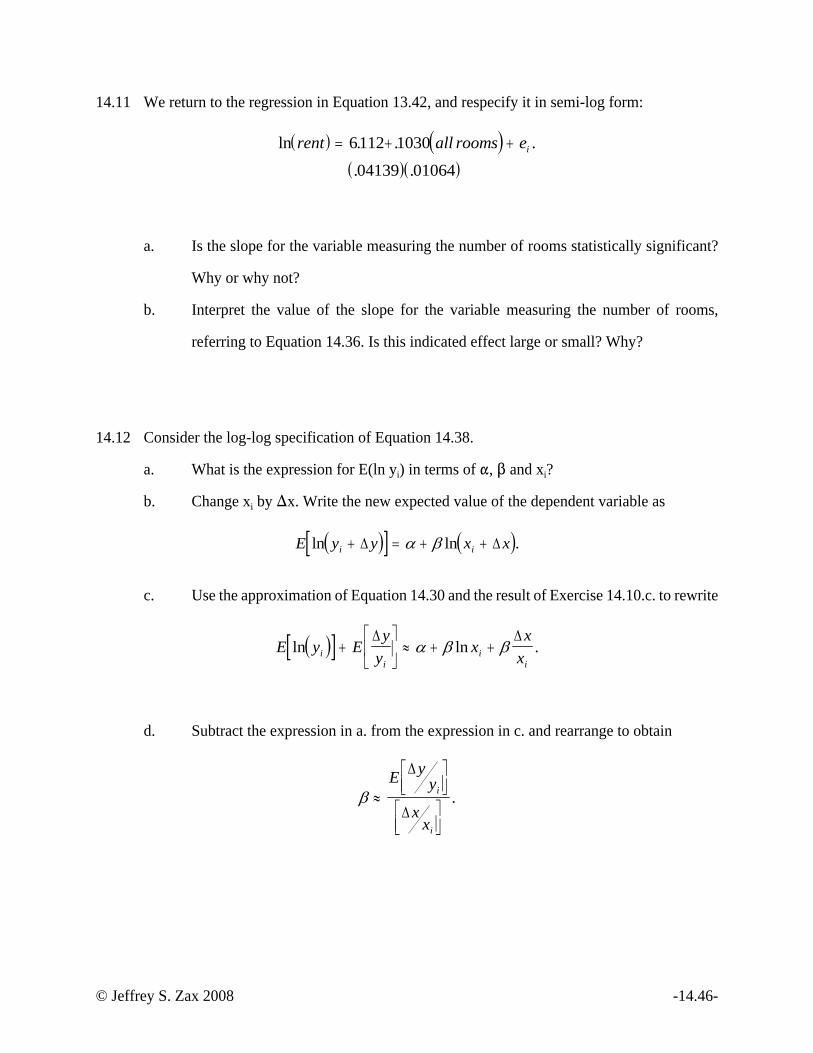
© Jeffrey S. Zax 2008 -14.46-

14.11 We return to the regression in Equation 13.42, and respecify it in semi-log form:

( ) ( )( )( )

ln . . .

. .

rent all rooms ei= + +6112 1030

04139 01064

a. Is the slope for the variable measuring the number of rooms statistically significant?

Why or why not?

b. Interpret the value of the slope for the variable measuring the number of rooms,

referring to Equation 14.36. Is this indicated effect large or small? Why?

14.12 Consider the log-log specification of Equation 14.38.

a. What is the expression for E(ln yi) in terms of ", $ and xi?

b. Change xi by )x. Write the new expected value of the dependent variable as

( )[ ] ( )E y y x xi iln ln .+ = + +Δ Δα β

c. Use the approximation of Equation 14.30 and the result of Exercise 14.10.c. to rewrite

( )[ ]E y Ey

yx

xxi

ii

iln ln .+

⎡

⎣⎢

⎤

⎦⎥ ≈ + +

Δ Δα β β

d. Subtract the expression in a. from the expression in c. and rearrange to obtain

β ≈

⎡⎣⎢

⎤⎦⎥

⎡⎣⎢

⎤⎦⎥

E yy

xx

i

i

Δ

Δ.

© Jeffrey S. Zax 2008 -14.47-

14.13 If we respecify the regression of Equation 14.34 in the log-log form of Equation 14.35, we

obtain

( )( )

( ) ( )

ln

. . ln .

. .

Gross National Income per capita

Corruption Perceptions Index ei

=

+ +6 394 1733

2323 1590

a. Is the slope for the natural log of the Corruption Perceptions Index statistically

significant? Why or why not?

b. Interpret the value of the slope for the natural log of the Corruption Perceptions Index,

referring to Equation 14.39. Is this elasticity big or small? Why?

14.14 Demonstrate that the population relationship of Equation 12.1 forces the effects of race to be

identical regardless of sex.

a. Subtract Equation 14.42 from Equation 14.44 to derive the expected earnings difference

between a black and a non-black man.

b. Subtract Equation 14.43 from Equation 14.45 to derive the expected earnings difference

between a black and a non-black woman.

c. Compare the answers to a. and b.

d. Make the comparison of a. for the interacted specification of Equation 14.48, using

Equations 14.53 and 14.55. Is the result the same as in a.?

e. Make the comparison of b. for the interacted specification of Equation 14.48, using

Equations 14.54 and 14.56. Is the result the same as in b.?

© Jeffrey S. Zax 2008 -14.48-

14.15 Return to Equation 14.49. Change x2i by )x2 . Follow the derivation in Equations 14.50 through

14.52 to prove that

ΔΔ

yx

x i2

2 3 1= +β β .

14.16 Return to Equations 14.59 and 14.60.

a. Test whether or not the three slopes in Equation 14.59 are statistically significant. What

do these tests indicate about the effect of being a black woman on expected earnings?

b. Test whether or not the three slopes in Equation 14.60 are statistically significant. What

do these tests indicate about the effect of being a black woman on expected earnings?

c. For the regression of Equation 14.60, the F-statistic for the test of the joint null

hypothesis H0: $2+$3=0 is .08. The degrees of freedom are 1 and 179,545. Using

Appendix table 3, interpret the results of this test. What does this test indicate about the

effect of being a black woman on expected earnings?

d. In Equation 13.30, footnote 10 of Chapter 13 and Exercise 13.12, we assert that any F-

test with a single degree of freedom in the numerator can be reformulated as a t-test.

Consider the population relationship

y x x xi i i i i= + + + +α β β β ε1 1 2 2 3 3 .

where x1i is a dummy variable identifying women, x2i is a dummy variable identifying

black men and x3i is a dummy variable identifying black women. Compare the expected

values of earnings for non-black men, non-black women, black men and black women

to those of Equations 14.53 through 14.56. Explain why this specification is equivalent

to that of Equation 14.48, where x1i is a dummy variable identifying women and x2i is

a dummy variable identifying blacks.

e. The sample regression that corresponds to the population relationship of d., calculated

© Jeffrey S. Zax 2008 -14.49-

with the sample of Equation 14.60, is

( ) ( ) ( )( ) ( ) ( ) ( )

earnings female black male black female error= − − − +40 784 19 581 14 520 167 2

1534 218 7 620 2 610 3

, , , . .

. . . .

How do the effects for females, black males and black females compare in the two

regressions? Are they statistically significant? Interpret them. In this equation, what

is the statistical test for the null hypothesis that expected earnings are the same for

black and non-black females? What is the outcome of this test?

f. In both of Equations 14.59 and 14.60, women and black men have large negative

slopes. This suggests the null hypothesis that their expected earnings might differ from

those of males by the same amount, H0: $1=$2. The F-statistic for the test of this null

hypothesis in Equation 14.59 is .55, with 1 and 996 degrees of freedom. For Equation

14.60, it is 66.46 with 1 and 179,545 degrees of freedom. What can we conclude

regarding this hypothesis?

g. The F-tests of f. have only one degree of freedom in the numerator. How would we

specify a regression in order to test the null hypothesis with a t-statistic?

14.17 Consider the sample regression of Equation 14.58, where x1i is a dummy variable and x2i is a

continuous variable:

y a b x b x b x x ei i i i i i= + + + +1 1 2 2 3 1 2 .

Imagine that x1i identifies women. Section 14.2 explains why we don’t want to add a dummy

variable identifying men, say x3i, to this regression. However, how do we know whether or not

the effect of x2i is different for men than for women? Is there a reason why we shouldn’t add

an interaction term between x2i and x3i to this regression, so that it looks like

y a b x b x b x x b x x ei i i i i i i i= + + + + +1 1 2 2 3 1 2 4 3 2 ?

© Jeffrey S. Zax 2008 -14.50-

a. Recall that x1i=0 when x3i=1, and x1i=1 when x3i=0. Prove that, for each observation,

x x x x xi i i i i2 1 2 3 2= + .

b. Consider the following auxiliary regression:

x a b x x b x x errori x x i i x x i i i2 1 2 3 22 1 2 3= + + + .

Prove that if a=0, and , this regression would fit perfectly: allbx x2 11= bx x2 3

1=

errors would be equal to zero.

c. Explain intuitively why the regression of Chapter 12 would choose the values

a=0, and if we were to actually calculate this regression.bx x2 11= bx x2 3

1=

d. Recall our discussion in Section 12.4. There we demonstrate that the multivariate

regression uses only the part of each explanatory variable that is not associated with any

of the other explanatory variables. Based on the answer to c., explain why x2i has no

parts that are not related to x1ix2i and x3ix2i.

e. Based on the answer to d., explain why, intuitively, the regression with which this

question begins cannot be calculated.

f. Return to Table 1.4. The regression there contains interaction terms for age and women,

and for age and men. It can be calculated because it omits a crucial variable. What is

this variable?

g. This analysis shows that there are two specifications that can be calculated. Regression

can estimate either the general effect of x2i and the difference between the effects of x2i

when x1i=0 and x1i=1, as in Section 14.5, or the absolute effects of x2i when x1i=0 and

x1i=1, as in Table 1.4. However, it cannot estimate a general effect and separate

absolute effects for each of the cases x1i=0 and x1i=1. Explain, intuitively, why.

© Jeffrey S. Zax 2008 -14.51-

14.18 The regression of Equation 14.61, omitting the interaction between the dummy variable

identifying women and the continuous variable for years of schooling, is

( ) ( )( ) ( ) ( )

earnings female yearsof schooling= − − +8 506 17 644 3 801

4 630 2 495 3411

, , , .

, , .

Explain, with reference to Section 12.2, why the addition of the interaction term in Equation

14.61 changes these results.

14.19 The intercept and slopes in Equation 14.62 appear to differ substantially in magnitude from

those in Equation 14.63. Is this because the two regressions are contradictory, or because some

estimates are not very precise? Form the confidence intervals around a, b1 and b2 of Equation

14.62. Do they include the corresponding values from 14.63? What is the best explanation for

the discrepancies between the two Equations?