chapter 14 hyperbolic geometry - cornell universitypi.math.cornell.edu/~web4520/cg-14-f2017.pdf ·...

Chapter 14

Hyperbolic geometry Math 4520, Fall 2017

So far we have talked mostly about the incidence structure of points, lines and circles. Butgeometry is concerned about the metric, the way things are measured. We also mentionedin the beginning of the course about Euclid’s Fifth Postulate. Can it be proven from the theother Euclidean axioms?

This brings up the subject of hyperbolic geometry. In the hyperbolic plane the parallelpostulate is false. If a proof in Euclidean geometry could be found that proved the parallelpostulate from the others, then the same proof could be applied to the hyperbolic plane toshow that the parallel postulate is true, a contradiction. The existence of the hyperbolicplane shows that the Fifth Postulate cannot be proven from the others. Assuming thatMathematics itself (or at least Euclidean geometry) is consistent, then there is no proof ofthe parallel postulate in Euclidean geometry. Our purpose in this chapter is to show thatTHE HYPERBOLIC PLANE EXISTS.

14.1 A quick history with commentary

In the first half of the nineteenth century people began to realize that that a geometry withthe Fifth postulate denied might exist. N. I. Lobachevski and J. Bolyai essentially devotedtheir lives to the study of hyperbolic geometry. They wrote books about hyperbolic geometry,and showed that there there were many strange properties that held. If you assumed thatone of these strange properties did not hold in the geometry, then the Fifth postulate couldbe proved from the others. But this just amounted to replacing one axiom with anotherequivalent one. These people simply assumed that there was such a non-Euclidean hyperbolicgeometry. For all they knew, they could have been talking about the empty geometry, provingwonderful theorems about beautiful structures that do not exist. It has happened in otherareas of Mathematics. Even the great C. F. Gauss only explored what might happen if thisnon-Euclidean geometry were really there. However, Gauss never actually published whathe found, possibly out of fear of ridicule.

Nevertheless, by the middle of the nineteenth century the existence of the hyperbolicplane, even with its strange properties, came to be accepted, more or less. I think thatis an example of the “smart people” argument, a variation of proof by intimidation. Ifenough smart people have tried to find a solution to a problem and they do not succeed,then the problem must not have a solution. (Note that it was felt that Watt’s problemcould not be solved either...until it was found.) In their defense, though, one could argue

1

2 CHAPTER 14. HYPERBOLIC GEOMETRY MATH 4520, FALL 2017

that any geometry and any mathematical system cannot really be proven to be consistantin an absolute sense. There has to be some sort basic principles and axioms that have to beassumed. Gauss, Bolyai, and Lobachevski could argue that they just based their theory on asystem other than Euclidean geometry. But later in the nineteenth century the foundationsof all of mathematics were examined and greatly simplified. This is why we study set theoryas invisioned by such people as Richard Dedekind. And as we have seen, the foundationsof Euclidean geometry were carefully examined by Hilbert. Euclidean geometry, howevercomplicated, was certainly as consistant as set theory. I do not see how such a statement canbe made about hyperbolic geometry, without some very convincing argument.

But that argument was found. In 1868, E. Beltrami actually proved that one can constructthe hyperbolic plane using standard mathematics and Euclidean geometry. Perhaps it cameas an anti-climax, but from then on though, hyperbolic geometry was less of a mystery andpart of the standard geometric repertoire. The ancient problem from Greek geometry “Canthe Fifth postulate be proved from the others?” had been solved. The Fifth postulate cannotbe proved.

We will present a construction for the hyperbolic plane that is a bit different in spiritfrom Beltrami’s, and is in the spirit of Klein’s philosophy, concentrating on the group ofthe geometry. This uses a seemingly unusual method, due to H. Minkowskii, that uses ananalogue to an inner product that has non-zero vectors with a zero norm. Odd as that mayseem, these ideas were fundamental to Einstein’s special theory of relativity.

14.2 A little algebra

We will be working with special conics and quadratic curves and this brings up symmetricmatrices. We will need some special information about these matrices.

A square matrix S is called symmetric if ST = S, where ()T denotes the transpose of amatrix.

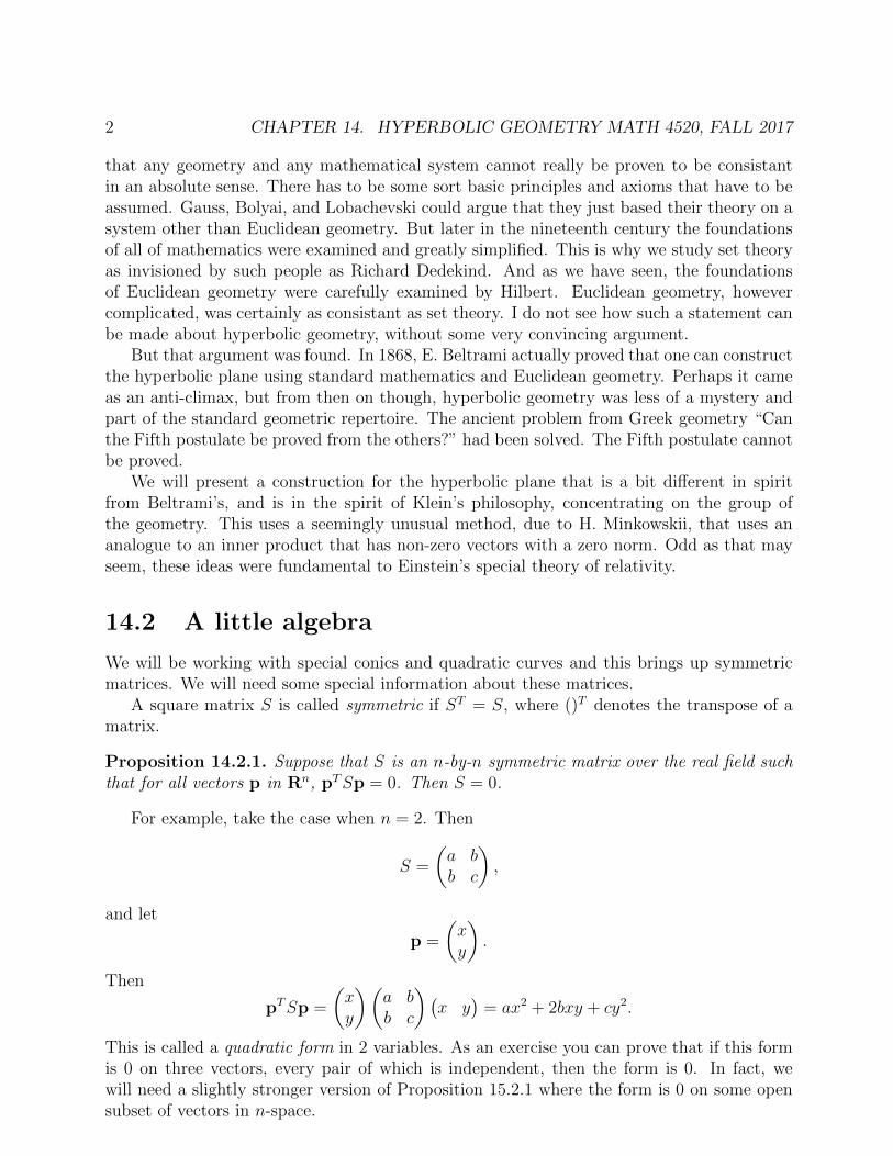
Proposition 14.2.1. Suppose that S is an n-by-n symmetric matrix over the real field suchthat for all vectors p in Rn, pTSp = 0. Then S = 0.

For example, take the case when n = 2. Then

S =

(a bb c

),

and let

p =

(xy

).

Then

pTSp =

(xy

)(a bb c

)(x y

)= ax2 + 2bxy + cy2.

This is called a quadratic form in 2 variables. As an exercise you can prove that if this formis 0 on three vectors, every pair of which is independent, then the form is 0. In fact, wewill need a slightly stronger version of Proposition 15.2.1 where the form is 0 on some opensubset of vectors in n-space.

14.3. THE HYPERBOLIC LINE AND THE UNIT CIRCLE 3

14.3 The hyperbolic line and the unit circle

We need to study the lines in the hyperbolic plane, and in order to understand this we willwork by analogy with the unit circle that is used in spherical geometry. We define them asfollows:

The Unit Circle

S1 =

{(xy

)| x2 + y2 = 1

}The Unit Circle The Hyperbolic Line

~

'...4'! ",

,",.

,

~

-t' ",/JFigure 15.3.1

We re~"rite these conditions in terms of matrices as follows:

The Circle The Hyperbola

For every p and q in R 2 define a "bi-

linear form " by

For ever)' p and q in R 2 define a "bi-

linear form " by

(p, q) = pfq, (p, q} = pf Dq,

",here p and q are regarded as column

vectors. So

\\there p and q are regarded as column

vectors and

{p, p) = -1}

wherext

/I'

~"

The Hyperbolic Line

H1 =

{(xt

)| x2 − t2 = −1, t > 0

}The Unit Circle The Hyperbolic Line

~

'...4'! ",

,",.

,

~

-t' ",/JFigure 15.3.1

We re~"rite these conditions in terms of matrices as follows:

The Circle The Hyperbola

For every p and q in R 2 define a "bi-

linear form " by

For ever)' p and q in R 2 define a "bi-

linear form " by

(p, q) = pfq, (p, q} = pf Dq,

",here p and q are regarded as column

vectors. So

\\there p and q are regarded as column

vectors and

{p, p) = -1}

wherext

/I'

~"

We rewrite these conditions in terms of matrices as follows:

The CircleFor every p and q in R2 define a “bilinearform” by

〈p,q〉 = pTq,

where p and q are regarded as column vectors.So

S1 = {p ∈ R2 | 〈p,p〉 = 1}

where

p =

(xy

).

The HyperbolaFor every p and q in R2 define a “bilinearform” by

〈p,q〉 = pTDq,

where p and q are regarded as column vectorsand

D =

(1 00 −1

).

SoH1 = {p ∈ R2 | 〈p,p〉 = −1}

where

p =

(xt

).

There should be no confusion between the two bilinear forms since one is used only in thecontext of the circle and the other is used only in the context of the hyperbola. In the caseof the circle, the bilinear form is the usual dot product.

One important difference between the two bilinear forms is that the form in the case ofthe hyperbola has vectors p such that 〈p,p〉 = 0, but p 6= 0. These are the vectors (calledisotropic vectors) that lie along the asymptotes that are the dashed lines in the Figure forthe hyperbolic line.


14.4 The group of transformations

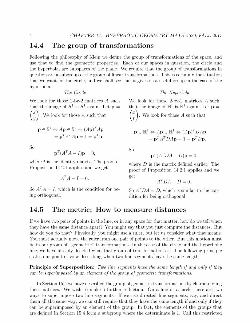
Following the philosophy of Klein we define the group of transformations of the space, anduse that to find the geometric properties. Each of our spaces in question, the circle andthe hyperbola, are subspaces of the plane. We require that the group of transformations inquestion are a subgroup of the group of linear transformations. This is certainly the situationthat we want for the circle, and we shall see that it gives us a useful group in the case of thehyperbola.

The Circle

We look for those 2-by-2 matrices A suchthat the image of S1 is S1 again. Let p =(xy

). We look for those A such that

p ∈ S1 ⇔ Ap ∈ S1 ⇔ (Ap)TAp

= pTATAp = 1 = pTp.

SopT (ATA− I)p = 0,

where I is the identity matrix. The proof ofProposition 14.2.1 applies and we get

ATA− I = 0.

So ATA = I, which is the condition for be-ing orthogonal.

The Hyperbola

We look for those 2-by-2 matrices A suchthat the image of H1 is H1 again. Let p =(xt

). We look for those A such that

p ∈ H1 ⇔ Ap ∈ H1 ⇔ (Ap)TDAp

= pTATDAp = 1 = pTDp.

SopT (ATDA−D)p = 0,

where D is the matrix defined earlier. Theproof of Proposition 14.2.1 applies and weget

ATDA−D = 0.

So ATDA = D, which is similar to the con-dition for being orthogonal.

14.5 The metric: How to measure distances

If we have two pairs of points in the line, or in any space for that matter, how do we tell whenthey have the same distance apart? You might say that you just compute the distances. Buthow do you do that? Physically, you might use a ruler, but let us consider what that means.You must actually move the ruler from one pair of points to the other. But this motion mustbe in our group of “geometric” transformations. In the case of the circle and the hyperbolicline, we have already decided what that group of transformations is. The following principlestates our point of view describing when two line segments have the same length.

Principle of Superposition: Two line segments have the same length if and only if theycan be superimposed by an element of the group of geometric transformations.

In Section 15.4 we have described the group of geometric transformations by characterizingtheir matrices. We wish to make a further reduction. On a line or a circle there are twoways to superimpose two line segments. If we use directed line segments, say, and directthem all the same way, we can still require that they have the same length if and only if theycan be superimposed by an element of the group. In fact, the elements of the groups thatare defined in Section 15.4 form a subgroup where the determinate is 1. Call this restricted

14.5. THE METRIC: HOW TO MEASURE DISTANCES 5

group the positive transformations. These are the transformations that can be regarded asthe rotations of the circle or the translations of the hyperbolic line.

These positive transformations also have the property that there is a unique (positive)transformation that takes one point to another. Indeed, we can use our superposition princi-ple by bringing all our directed line segments back to a fixed canonical position, which we callParis, in order to compare lengths. For a while Paris did keep a fixed meter length that wasused for comparison the world over. So there is a unique positive geometric transformationthat takes a point to Paris. Alternatively, we can think of Paris being transformed to anygiven point θ by a positive transformation Aθ. We present Aθ explicitly and define Paris.

The Circle

Let Paris =

(10

). Then

Aθ =

(cos θ − sin θsin θ cos θ

).

So Aθ on S1 is identified with(cos θ − sin θsin θ cos θ

)(10

)=

(cos θsin θ

).

The Hyperbola

Let Paris =

(01

). Then

Aθ =

(cosh θ sinh θsinh θ cosh θ

).

where the hyperbolic functions are definedby

cosh θ = (eθ + e−θ)/2

sinh θ = (eθ − e−θ)/2.

So Aθ on H1 is identified with(cosh θ sinh θsinh θ cosh θ

)(01

)=

(sinh θcosh θ

).

We leave it as an easy exercise to show that these matrices Aθ satisfy the orthogonal andhyperbolic orthogonal conditions described in Section 14.4. Figure 14.1 shows the “ruler” incircle geometry as well as hyperbolic geometry.

CLASSICAL GEOMETRIES6

The Hyperbola

Let Paris =

cosGsinG

-sin 6cos6

cash 8

sinh 8

sinh 8cash 8

AB = AB =

where the hyperbolic functions are de-fined by

So As on 81 is identified with

cosBsinB

-sin 8 \ ( 1 \ = ( C?S 8 \cos8) 0) sm8 ) coshB = (e8 + e-8)/2

sinhB = (e8 -e-8)/2.

So AB on HI is identified with

sinh 8 \ ( 0 \ = ( sinh 8 \cosh8) \1) \cosh8)

cosh esinh e

We leave it as an easy exercise to show that these matrices AB satisfy the orthogonaland hyperbolic orthogonal conditions described in Section 15.4. Figure 15.5.1 shows the"ruler" in circle geometry as well as hyperbolic geometry.

In terms of the ordinary Euclidean distance, multiples of 8 grow exponentially on thehyperbolic line, whereas on the circle the multiples of 8 appear at fixed intervals aroundthe circle. Notice also that the isotropic directions

(~) and (-i)

are also independent eigenvectors of AB, with eigenvalues eB /2 and e-B /2 respectively.

Figure 14.1

In terms of the ordinary Euclidean distance, multiples of θ grow exponentially on the


hyperbolic line, whereas on the circle the multiples of θ appear at fixed intervals around thecircle. Notice also that the isotropic directions(

11

)and

(−11

)are also independent eigenvectors of Aθ, with eigenvalues eθ/2 and e−θ/2 respectively.

14.6 Computing length from coordinates

In Section 14.5 we saw how to compute distances by moving rulers around, but it would behelpful if we could assign a real number that was the distance between any pair of points inour space. Philosophically, we want this distance to “look like” the distance along a line. Wedescribe this as follows:

Principle of Juxtaposition: The length of two intervals on a line, put end-to-end, is thesum of the lengths of the two intervals.

This principle does not strictly hold for the circle, which is one reason that spherical ge-ometry or elliptic geometry does not even satisfy the first few axioms of Euclid. Nevertheless,this principle does hold “in the small”, namely when the intervals are both sufficiently small.In hyperbolic geometry, this principle does hold and it tells us how to compute distances.

In either case, suppose that θ1 and θ2 are two points, both in S1 or both in H1. We canregard θ1 and θ2 as points on a line, but we must figure out how to add their lengths fromParis, say. One way is to arrange it so that θ1 + θ2 is that point where

Aθ1+θ2 = Aθ1 + Aθ2 .

It is easy to check that this equation is satisfied by the circular functions, sine and cosine,on the one hand, and the hyperbolic sine and hyperbolic cosine, on the other hand. So thedistance between θ1 and θ2 is just |θ1 − θ2| with the given parametrizations.

We observe that the transformations A that were found in Section 14.4 not only willserve as the distance-preserving transformations, of the circle or hyperbolic line, but also“preserve” the inner product for these spaces in the following sense:

The Circle

If p and q are on S1, for an orthogonal trans-formation A,

〈p,q〉 = pTq = pTATAq = 〈Ap, Aq〉.

The HyperbolaIf p and q are on H1, for a hyperbolic trans-formation A satisfying the condition of Sec-tion 14.4,

〈p,q〉 = pTDq = pTATDAq = 〈Ap, Aq〉.

Suppose p and q are two points, where we know their Cartesian coordinates, as wehave described above. What is their distance? From the principle of Juxtaposition and theconstruction of our matrices A, we assume they preserve the distances between points. Wewill calculate that distance in terms of the coordinates of p and q using the inner productin each case. In order to make the calculation easier we will bring the interval between themback to Paris, where p is at Paris and q corresponds to the position at θ. Then d(p,q) = θ.

14.7. AN EXTRA DIMENSION 7

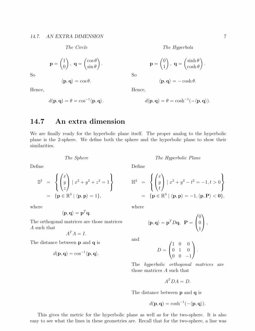
The Circle

p =

(10

), q =

(cos θsin θ

).

So〈p,q〉 = cos θ.

Hence,

d(p,q) = θ = cos−1〈p,q〉.

The Hyperbola

p =

(01

), q =

(sinh θcosh θ

).

So〈p,q〉 = − cosh θ.

Hence,

d(p,q) = θ = cosh−1(−〈p,q〉).

14.7 An extra dimension

We are finally ready for the hyperbolic plane itself. The proper analog to the hyperbolicplane is the 2-sphere. We define both the sphere and the hyperbolic plane to show theirsimilarities.

The Sphere

Define

S2 =

xyz

| x2 + y2 + z2 = 1

= {p ∈ R3 | 〈p,p〉 = 1},

where〈p,q〉 = pTq.

The orthogonal matrices are those matricesA such that

ATA = I.

The distance between p and q is

d(p,q) = cos−1〈p,q〉.

The Hyperbolic Plane

Define

H2 =

xyt

| x2 + y2 − t2 = −1, t > 0

= {p ∈ R3 | 〈p,p〉 = −1, 〈p,P〉 < 0},

where

〈p,q〉 = pTDq, P =

001

,

and

D =

1 0 00 1 00 0 −1

.

The hyperbolic orthogonal matrices arethose matrices A such that

ATDA = D.

The distance between p and q is

d(p,q) = cosh−1(−〈p,q〉).

This gives the metric for the hyperbolic plane as well as for the two-sphere. It is alsoeasy to see what the lines in these geometries are. Recall that for the two-sphere, a line was


z

y

x

Figure 14.2

defined to be the intersection of a plane through the origin with the two-sphere. In the case ofthe hyperbolic plane practically the same definition works. Namely, a line is the intersectionof a plane through the origin with H2, the hyperboloid of revolution as defined above.

In both of these cases it is easy to see that any line can be transformed by an elementof the group of geometric transformations to the circle or line that we defined previouslyin earlier sections. In the case of S2, rotations about each of the x-axis, y-axis, and z-axisgenerate the group of positive transformations. In the case of H2 the following matricesgenerate the hyperbolic transformations:

cosh θ 0 sinh θ0 1 0

sinh θ 0 cosh θ

,

1 0 00 cosh θ sinh θ0 sinh θ cosh θ

,

cos θ − sin θ 0sin θ cos θ 0

0 0 1

.

Note that the last matrix is the usual Euclidean rotation matrix with sines and cosines.This is because those matrices only operate on the the first two coordinates and the innerproduct is the usual Euclidean inner product with all positive coefficients.

In fact we now have the complete definition of the hyperbolic plane that is the notoriouscompetitor of the Euclidean plane for satisfying the axioms of Euclidean geometry, exceptfor the Fifth postulate. We have defined distances, but it follows (and is straightforward todo) that angles can also be defined for the hyperbolic plane. Bring everything to Paris, andmeasure it there.

14.8 Area in the hyperbolic plane

One of the most striking features of the hyperbolic plane is the behavior of areas. First wecalculate the area of a spherical disk, using an old theorem of Archimedes, and then apply asimilar argument to calculate the area of a hyperbolic disk.

Because of the homogeneity of the group of isometries of the unit sphere, we can assumethat the disk is centered at the north pole, and the angle φ, as in spherical coordinates, inFigure 14.3 below, the radius of the spherical disk is shown. Then the circumference Cφ of

14.8. AREA IN THE HYPERBOLIC PLANE 9

the disk of radius φ, Dφ is Cφ = 2π sinφ. Then the area of the disk is

Aφ =

∫ φ

0

2π sinx dx = 2π(1− cosφ).

This implies the following theorem of Archimedes.

Theorem 14.8.1. The area of a region in the unit sphere S2 is the same as the correspondingregion projected laterally out to the unit radius cylinder circumscribing the sphere.

Figure 14.3

A similar construction holds in the case of the hyperboloid. In Figure 14.4 the point P onthe t−x axis has coordinates (sinhφ, 0, coshφ), where φ is the radius of the disk Dφ centeredat Paris (0, 0, 1). Since the circumference Cφ of Dφ is horizintal, Cφ = 2π sinhφ. So the areaof Dφ is

Aφ =

∫ φ

0

2π sinhx dx = 2π(coshφ− 1).

So the lateral projection of the hyperbolic plane onto the upper part of the unit cylinderabove Paris, will be an equal-area projection as before.

In this hyperbolic case, the area of a hyperbolic disk grows exponentially with the radiusφ, since the area is roughly 2π coshφ which is roughly πeφ, since e−φ is extremely small forlarge φ. For example, if one adds annulus of width 1 to a hyperbolic disk, that area will beroughly πeφ+1, and since πeφ+1/πeφ = e, that annular region has more area than the originalregion itself.


Figure 14.4

14.9 The Klein-Beltrami model

An important feature of the hyperbolic plane is the property that it does not satisfy Euclid’sFifth postulate. How do we see this? Simply look at H2. A good vantage point is the origin.Project H2 from the origin into the plane t = 1. Define this central projection π : H2 → R2

by

π

xyt

=

x/ty/t1

.

It is easy to see that π is a one-to-one function and that the image of H2 is the interior ofthe unit disk in the plane t = 1. See Figure 14.5.

Since a line in H2 is the intersection of a plane through the origin with H2 itself, theprojection of a line is an open line segment in the unit disk in the plane t = 1. It is easyto see that given any point p and a line L not containing that point, there are many linesthrough p not intersecting L. See Figure 14.6.

We can use the formula in Section 14.7 to define distances in the Klein-Beltrami model.H2 projects onto the interior of the unit disk

B =

xy

1

| x2 + y2 = 1

.

14.10. HYPERBOLIC INVERSION 11HYPERBOLIC GEOMETRY 11

t

p

~~

/

~x,

,/ ,

/~s.Figure 15.8.1

Since a line in H2 is the intersection of a plane through the origin with H2 itself, the

projection of a line is an open line segment in the unit disk in the plane t = 1. It is easy

to see that given any point p and a line L not containing that point, then there are many

lines through p not intersecting L. See Figure 15.8.2.

Figure 15.8.2

In this model we see that the hyperbolic distance between two points p and q is

d(p,q) = 2sinh-1 ~~..;(7r-lp -7r-lq, 7r-lp -7r-lq} ~ .

We could use the above formula to define distances in this Klein model directly if we

wished. Beltrami used a different approach that is common in differential geometry. He

defined a real valued function at each point in the unit disk, and then the distance along a

curve is obtained by integrating that function along the curve. The distance between two

points is the shortest hyperbolic length of a curve between the two points.

Figure 14.5

HYPERBOLIC GEOMETRY 11

t

p

~~

/

~x,

,/ ,

/~s.Figure 15.8.1

Since a line in H2 is the intersection of a plane through the origin with H2 itself, the

projection of a line is an open line segment in the unit disk in the plane t = 1. It is easy

to see that given any point p and a line L not containing that point, then there are many

lines through p not intersecting L. See Figure 15.8.2.

Figure 15.8.2

In this model we see that the hyperbolic distance between two points p and q is

d(p,q) = 2sinh-1 ~~..;(7r-lp -7r-lq, 7r-lp -7r-lq} ~ .

We could use the above formula to define distances in this Klein model directly if we

wished. Beltrami used a different approach that is common in differential geometry. He

defined a real valued function at each point in the unit disk, and then the distance along a

curve is obtained by integrating that function along the curve. The distance between two

points is the shortest hyperbolic length of a curve between the two points.

Figure 14.6

So for p,q ∈ B, their Klein-Beltrami distance is

d(p,q) = cosh−1

⟨−p√−〈p,p〉

,q√−〈q,q〉

⟩.

This is obtained by projecting back up to H2 and using the distance we calculated there.Beltrami used a different approach that is common in differential geometry. He defined areal valued function at each point in the unit disk, and then the distance along a curve isobtained by integrating that function along the curve. The distance between two points isthe shortest hyperbolic length of a curve between the two points.

14.10 Hyperbolic inversion

Just as inversion in Euclidean space and plane has very convenient properties, so there isa notion of inversion for the indefinite inner product that is used to define the hyperbolic


plane. Let

xyt

= p be a point in R3, but not on the (light) cone x2 +y2− t2 = 0. We define

inversion as

β(p) =

x/(x2 + y2 − t2)y/(x2 + y2 − t2)t/(x2 + y2 − t2)

.

Let H be the collection of quadric surfaces of the form

x2 + y2 − t2 + ax+ by + ct+ d = 0,

for some constants a, b, c, d. We claim the following:

(a) β(β(p)) = p

(b) β(p) = p for p ∈ H2.

(c) If S ∈ H, then β(S) ∈ H or β(S) is a plane.

(d) If S1,S2 ∈ H, then S1 ∩ S2 ⊂ P , a plane in R3.

(e) If S ∈ H, then S ∩ {(x, y, c) | c = constant} is a circle.

Properties (a) and (b) are easy to check. For Property (c), we calculate:

x2

(x2 + y2 − t2)2+

y2

(x2 + y2 − t2)2− t2

(x2 + y2 − t2)2

+ax

(x2 + y2 − t2)+

by

(x2 + y2 − t2)+

ct

(x2 + y2 − t2)+ d = 0.

Clearing we get:

x2

(x2 + y2 − t2)+

y2

(x2 + y2 − t2)− t2

(x2 + y2 − t2)+ ax+ by + ct+ d(x2 + y2 − t2) =

1 + ax+ by + ct+ d(x2 + y2 − t2) = 0.

Thus β(S) ∈ H when d 6= 0, and is a plane when d = 0.For Property (d) in S1 ∩ S2 the quadratic terms cancel leaving only the linear termes.For Property (e), it is clear that when the t coordinate is constant, the equation for the

subset of H is a circle.

Let H1 = {

xyt

| x2 + y2 − (t − 1/2)2 = −1/4}, which is a surface in H through Paris001

and the origin 0. Note that the origin 0 ∈ H1, so by the proof of (c), β(H1) is a plane,

and by (b), Paris is in the plane, which is tangent to both H1 and H2 and thus it is thehorizontal plane t = 1. This is shown in Figure 14.7, where the projection from the uppercomponent of H1 into the plane is shown (as f(x). When this figure is rotated about the

14.10. HYPERBOLIC INVERSION 13

Figure 14.7: This shows, in the x−t plane the hyperbolic inversion of the red hyperbolaabout the the blue hyperbola. The image of upper red hyperbola is interval betweenthe two dashed blue asymptotes.

t-axis you get a figure something like Figure 14.8, but where the disk is translated down tothe x − y plane. Note that here the red hyperbola, when rotated about the t-axis, is thestandard hyperboloid for the hyperbolic plane, and the blue hyperbola, with the resultinghyperboloid, are used to understand the projection in Figure 14.7.

By (d) circles (including hyperbolic lines) are the intersection of planes with H2 and (e)their inversion/projection in the disk in the t = 1 plane will be actual circles, or in the caseof lines through Paris the image will be straight lines (through Paris). It turns out that thisimplies this inversion will be conformal. That is the angle between curves in H2 will be suchthat the angle between the corresponding image curves will also be the same. This image isthe Poincare model discussed next.

Note that when a hyperbolic line in H2 goes through Paris, its projection in the hyperbolicdisk will be a straight line. Any hyperbolic isometry of H2 corresponds to a circle preservingmap on the Poincare disk, and so must preserve the orthogonal intersection with the boundaryof the disk. Since any line H2 can be trenslated/rotated to any other line, all the circles inPoincare model corresponding to lines in H2 are orthogonal to the boundary of the disk.


14.11 The Poincare model

The Klein model of the hyperbolic plane has the property that hyperbolic lines are “straight”,but one might wish for other properties. We describe here a model, due to H. Poincare, thatis yet another equivalent description of the hyperbolic plane, but it has the pleasing propertythat hyperbolic circles are Euclidean circles.

For the Klein-Beltrami model we used central projection of H2 into the plane t = 1. Recallthat for the sphere S2 stereographic projection took circles to circles. We can apply the sameidea for H2 in our Minkowskii geometry. A natural place to choose for the projection point

is the antipode of Paris, namely

00−1

= S. See Figure 14.8.

CLASSICAL GEOMETRIES12

15.9 The Poincare modelThe Klein model of the hyperbolic plane has the property that hyperbolic lines are

"straight", but one might wish for other properties. We describe here a model, due to H.Poincare, that is yet another equivalent description of the hyperbolic plane, but it has thepleasing property that hyperbolic circles are Euclidean circles.

For the Klein-Beltrami model we used central projection of H2 into the plane t = 1.Recall that for the sphere 82 stereographic projection took circles to circles. We can applythe same idea for H2 in our Minkowskii geometry. A natural place to choose the projection

OO

-1= s. See Figure 15.9.1.point is the antipode of Paris, namely

t

p " // y

x

~~ ~

Figure 15.9.1

We define 11" 8 : H2 -+ R 2 by projection from 5 into the plane t = 0. The image ofH2 under 11" 8 is the unit disk again, but in the plane t = 0. But what is the image of ahyperbolic line? It turns out that they are circles in the unit disk that are orthogonal tothe boundary of the unit disk or they are diameters in the unit disk. So Figure 15.8.2 thenis transformed into Figure 15.9.2.

An important property of the Poincare model is that the angle between the circles thatare the image of two lines is the same as the angle between the lines in the hyperbolic planeH2 itself. We say that the model is conformal. (It is also true that stereographic projectionfrom the sphere 52 into the plane is conformal. The whole plane is the conformal imageof the sphere 52 minus one point. )

We show some tilings M. C. Escher based on this conformal property at the end of theChapter .

Figure 14.8

We define πs : H2 → R2 by projection from S into the plane t = 0. The image of H2

under πs is the unit disk again, but in the plane t = 0. But what is the image of a hyperbolicline? It turns out that they are circles in the unit disk that are orthogonal to the boundaryof the unit disk or they are diameters in the unit disk. So Figure 14.6 then is transformedinto Figure 14.9.

An important property of the Poincare model is that the angle between the circles thatare the image of two lines is the same as the angle between the lines in the hyperbolic planeH2 itself. We say that the model is conformal. (It is also true that stereographic projectionfrom the sphere S2 into the plane is conformal. The whole plane is the conformal image ofthe sphere S2 minus one point.)

We show some tilings of the hyperbolic plane, one by M. C. Escher that is conformal, andanother in the spirit of Escher, viewed in the Klein model, at the end of this Chapter.

14.12. AREA OF A TRIANGLE 15HYPERBOLIC GEOMETRY 13

Figure 15.9.2

Exercises:

1. Show that if a real bilinear form in two variables is O on three independent vectors,then is is the O form.

2. In any dimension, show that if a real bilinear form is O on an open set of vectors,then it is the O form.

3. Show that the circular functions, sine and cosine, satisfy the matrix product rulein Section 15.5. Do the same for the h)'perbolic functions.

4. Suppose that two lines in H2 are given by

Cl ) D ( ~ ) = al X + b1 y -Cl t = 0b1

c2)D (~) =a2x+b2y-C2t=O.b2

Find the angle between them.5. In Section 15.8 find an explicit representation of the inverse projection map 7r-l

that takes the unit disk onto H2.6. Consider the unit sphere tangent to a plane at its South Pole as in Figure 15.E.1.

Figure 14.9

14.12 Area of a triangle

Another object that one might like to find the area of is a triangle. The unusual thing aboutthe area of a unit radius spherical triangle and a hyperbolic triangle described here is thatthe area only depends on their internal angles, whereas in the Euclidean plane, there is ascaling that change the area even for triangles with fixed angles. First the spherical case.

Consider two half geodesics on the unit sphere that form a lune as shown in Figure 14.10.It is easy to see that if the angle between the geodesics is θ, since the area of the sphere is4π the area of the lune is 4πθ/2π = 2θ.

Figure 14.10: A lune viewed from the side and above

In order to see what the area of geodesic triangle is on the unit sphere, consider the ar-rangements of three geodesics on the sphere. Here it helps to use the stereographic projectionin the plane in Figure 14.11, so we can identify the regions easily even though the areas ofthe planar regions are not related to the corresponding regions on the sphere.

If the spherical triangle has area A, with internal angles x, y, z, then the complementaryarea in each of the corresponding lunes is 2x − A, 2y − A, 2z − A, and the other spherical


Figure 14.11: A stereographic projection of three spherical geodesics bounding a spher-ical triangle with internal angles x, y, z.

triangle indicated by 2y − A is the antipode of the complementary triangle in the y lune.So adding up the areas of the four triangular areas constituting a hemisphere around the yangle, we get

A+ 2x− A+ 2y − A+ 2z − A = 2(x+ y + z)− 2A = 2π,

which implies A = x+ y + z − π, as desired.For a hyperbolic triangle, the calculation is very similar, but with some differences. First,

there is an infinite geodesic triangle that has finite area. This can be seen in the Poincaremodel where the edges meet at a point on the circle that represents the boundary of thePoincare disk as in Figure 14.12.

Theorem 14.12.1. All infinite geodesic triangles in the hyperbolic plane are congruent andhave finite area π.

This is somewhat surprising since such triangles are unbounded and have ”straight” sides.The fact that they all are congruent follows from what we know about the generators ofthe isometries of the hyperbolic plane. The various images in the Poincare model are notcongruent and they do not all have the same area, but, of course, we know that projection canchange areas and lengths, although for the stereographic projection angles and circles/linesare preserved. The crucial point is that the area is finite.

14.12. AREA OF A TRIANGLE 17

Figure 14.12: An infinite triangle withfinite area π in the Poincare model Figure 14.13: An infinite ideal polygon with

finite area (n− 2)π in the Poincare model.

Corollary 14.12.2. Any finite ideal polygon with n vertices on the boundary of the hyperbolicplane at infinity(as in Figure 14.13) has area (n− 2)π.

We continue this process to consider the case when a triangle has one internal angle whilethe two others are at the boundary. We can consider the case when the non-boundary angleis 2π/n, and is at the center of the disk. The symmetric polygon on the boundary at infinityhas area (n−2)π and so the area of each triangle is (n−2)π/n = π−2π/n. If we take k ≤ nof these polygons, their total area is k(π − 2π/n) = kπ − 2πk/n. If we chop off k − 1 of thepoints at infinity as in Figure 14.14 to get another triangle with one internal angle of 2π/n,whose area is kπ − 2πk/n − (k − 1)π = π − 2πk/n. Thus for any angle α that is a rationalmultiple of π, and by the continuity of area, for all α any triangle with only one internalangle α, its area is π − α.

Figure 14.14: This shows how to find the area of a triangle with just one non-zerointernal angle.

Theorem 14.12.3. If x, y, z are the internal angles of a hyperbolic triangle, its area isπ − (x+ y + z).

We can use an argument similar to that used for the spherical case shown in Figure 14.15.Here A+ π− x+ π− y−A+ π− z + π− x−A+ π− y + π− z −A = 4π, which reduces to−2A+ 6π − 2(x+ y + z) = 4π, and A = π − x+ y + z.


Figure 14.15: This shows how to find the area of a general triangle.

14.13 Exercises:

1. Show that if a real bilinear form in two variables is 0 on three independent vectors,then is is the 0 form.

2. In any dimension, show that if a real bilinear form is 0 on an open set of vectors, thenit is the 0 form.

3. Show that the circular functions, sine and cosine, satisfy the matrix product rule inSection 15.5. Do the same for the hyperbolic functions.

4. Suppose that two lines in H2 are given by

(a1 b1 c1

)D

xyt

= a1x+ b1y − c1t = 0

(a2 b2 c2

)D

xyt

= a2x+ b2y − c2t = 0.

Find the angle between them.

5. Consider the unit sphere tangent to a plane at its South Pole as in Figure 14.16.

14.13. EXERCISES: 19CLASSICAL GEOMETRIES14

North Pole

Figure 15.E.l

Projection parallel to the North-South axis of the sphere takes the unit diskcentered at the South Pole to the Southern Hemisphere. Stereographic projectionfrom the North Pole then takes the Southern Hemisphere onto the disk of radius 2centered at the South Pole, back in the plane. Show that the composition of thesetwo projections takes the Klein-Beltrami model of the hyperbolic plane onto thePoincare model of the hyperbolic plane.

Sho,v that the above composition of projections is also the same as the com-position of projections using central projection to H2 and then the hyperbolicstereographic projection back to the plane followed by simple multiplication by 2from the South Pole.

7. Sho\\' that the circumference of the disk in H2 of radius 8 is 271" sinh 8. This cir-cumference is the set of points of distance 8 from a fixed point. (Hint: Choosethe center point to be Paris, and think about what kind of circle you have in H2.)\\'fhat is the circumference of the disk of radius 8 in 82?

8. Use Problem 7 to show that the area of the disk of radius 8 in H2 is 271"( cosh 8 -1 ).You may use calculus. Think of a geometric way of finding the circumference of adisk by taking a derivative. What is the area of a disk of radius 8 in 82?

9. Use Problem 8 to calculate the area in H2 of the annular region between the circleof radius 8 and the circle of radius 8 + 1. What is the limit as 8 goes to infinity ofthe ratio of this annular area and the total area of the disk of radius 8 + 1 ? Whereis most of the area in a hyperbolic disk?

Figure 14.16

Projection parallel to the North-South axis of the sphere takes the unit disk centered atthe South Pole to the Southern Hemisphere. Stereographic projection from the NorthPole then takes the Southern Hemisphere onto the disk of radius 2 centered at theSouth Pole, back in the plane. Show that the composition of these two projectionstakes the Klein-Beltrami model of the hyperbolic plane onto the Poincare model of thehyperbolic plane.

Show that the above composition of projections is also the same as the compositionof projections using central projection to H2 and then the hyperbolic stereographicprojection back to the plane followed by simple multiplication by 2 from the SouthPole.

6. Show that the circumference of the disk in H2 of radius θ is 2π sinh θ. This circumferenceis the set of points of distance θ from a fixed point. (Hint: Choose the center point to beParis, and think about what kind of circle you have in H2.) What is the circumferenceof the disk of radius θ in S2?

7. Use Problem 6 to show that the area of the disk of radius θ in H2 is 2π(cosh θ − 1).You may use calculus. Think of a geometric way of finding the circumference of a diskby taking a derivative. What is the area of a disk of radius θ in S2?

8. Use Problem 7 to calculate the area in H2 of the annular region between the circle ofradius θ and the circle of radius θ + 1. What is the limit as θ goes to infinity of theratio of this annular area and the total area of the disk of radius θ+ 1? Where is mostof the area in a hyperbolic disk? (I like to call this the “Canada theorem” since this islike Canada, which has most of its population quite close to its boundary.)

9. Show how to define the “Gans” model of the hyperbolic plane where a line correspondsto one component of a hyperbola centered at the origin.

10. Find a general formula for the area of a hyperbolic polygon with geodesic sides in termsof the exterior angles.

11. Show that an isometry of the hyperbolic plane is determined uniquely by the image ofany three distinct points on the circle at infinity in the Poincare model.


12. Describe hyperbolic 3-space H3 and show that any isometry in the correspondingPoincare model is determined by the image of 3 points on the boundary sphere S2.

14.14 Escher pictures

Figure 14.17 is one of Escher’s popular “circle limits” which is a tiling of the hyperbolicplane viewed in the Poincare model. Figure 14.18 is a similar tiling, but viewed in theKlein-Beltrami model.

14.14. ESCHER PICTURES 21

Figure 14.17: Angels and Devils


RHW

Figure 14.18: Notice how circles become ellipses

chapter 14 hyperbolic geometry - cornell universitypi.math.cornell.edu/~web4520/cg-14-f2017.pdf ·...

Documents