chapter 15mpfrende/ecological genomics... · chapter 15 bioinformatics ... dedicated team of...

Chapter 15

Bioinformatics Analysis of Microarray Data

Yunyu Zhang, Joseph Szustakowski, and Martina Schinke

Abstract

Gene expression profiling provides unprecedented opportunities to study patterns of gene expressionregulation, for example, in diseases or developmental processes. Bioinformatics analysis plays an importantpart of processing the information embedded in large-scale expression profiling studies and for laying thefoundation for biological interpretation.Over the past years, numerous tools have emerged for microarray data analysis. One of the most popular

platforms is Bioconductor, an open source and open development software project for the analysis andcomprehension of genomic data, based on the R programming language.In this chapter, we use Bioconductor analysis packages on a heart development dataset to demonstrate

the workflow ofmicroarray data analysis from annotation, normalization, expression index calculation, anddiagnostic plots to pathway analysis, leading to a meaningful visualization and interpretation of the data.

Key words: Annotation, normalization, gene filtering, moderated F-test, GSEA, pathway analysis,affymetrix GeneChipTM, sigPathway.

1. Introduction

The purpose of this chapter is to provide an understanding of theroutine steps for microarray data analysis using Bioconductor (1)packages written in R (2), a widely used open source programminglanguage and environment for statistical computing and graphics.Both R and Bioconductor are under active development by adedicated team of researchers with a commitment to good doc-umentation and software design. We assume that the reader has abasic understanding about data structures and functions in Rprogramming. However, all of the analysis steps and toolsdescribed in this chapter have also been implemented in othersoftware packages (summarized in Section 4). The workflow

K. DiPetrillo (ed.), Cardiovascular Genomics, Methods in Molecular Biology 573,DOI 10.1007/978-1-60761-247-6_15, ª Humana Press, a part of Springer Science!Business Media, LLC 2009

259

shown in Fig. 15.1 facilitates the understanding of the basicprocedures in microarray data analysis and serves as an outline ofthis chapter.

2. Materials

2.1. Software R can be downloaded from http://www.r-project.org and beinstalled on all three mainstream operating systems (Windows,Mac, Unix/Linux). The general installation manual and introduc-tory tutorials can be obtained from the same website. Similar toother statistical software packages, R provides a statistical frame-work and terminal-based interface for users to input commands fordata manipulation. Additional packages (Table 15.1) from

ArrayImage

Cel File(raw probe-level expression data)

Probe-sets Level Expression &Detection calls

Normalization &Summarization

Differentially Expressed Genes

Gene Filtering

Clustering AnalysisPathway AnalysisMotif AnalysisGene Networks

Statistical Filtering

High Level Statistical Analysis

Fig. 15.1. Microarray data analysis work flow for Affymetrix GeneChipTM arrays.

Table 15.1List of add-on R packages required for analysis

Package Description

Affy (31) Basic functions for low-level analysis of Affymetrix GeneChipTM

oligonucleotide arrays

PLIER (5) Normalize and summarize the Affymetrix probe-level expression data usingthe PLIER method

LIMMA (32) Linear model for microarray analysis

sigPathway (12) Pathway (Gene-Set) analysis for high-throughput data

mm74av1mmentregcdf Entrez Gene-based chip definition file (CDF) for Affymetrix MG-74AV1platform

org.Mm.eg.db Annotation mapping based on mouse Entrez Gene identifiers

260 Zhang, Szustakowski, and Schinke

Bioconductor (http://www.bioconductor.org) are required priorto starting the analysis. Details about the package installation canbe found in Section 3.1. The R terminal output is highlightedthroughout the chapter in courier font.

2.2. Dataset A gene expression profiling experiment of heart ventricles at var-ious stages of cardiac development generated by the CardioGe-nomics Program for Genomic Applications (PGA) was used as atest dataset. This dataset can be downloaded from NCBI GeneExpression Omnibus (GEO; accession number GSE75). Itincludes seven time-points covering gene expression in the heartfrom embryonic stages through adolescence into adulthood(Table 15.2). Though this study was performed with an earlierAffymetrix platform (MGU-74Av1), the design of this study andquality of the data make this a valuable test dataset to this date.

3. Methods

3.1. R PackageInstallation

After downloading and installing R software (see Note 1), an Rterminal can be started to install the required Bioconductor coreand additional packages (see Note 2).>source("http://www.bioconductor.org/biocLite.R")>biocLite()Running biocinstall version 2.1.11 with R version 2.6.1Your version of R requires version 2.1 of Bioconductor.Will install the following packages:[1 ] "affy" "affydata" "affyPLM" "annaffy" "annotate"[6 ] "Biobase" "Biostrings" "DynDoc" "gcrma" "genefilter"

[11 ] "geneplotter" "hgu95av2" "limma" "marray" "matchprobes"[16 ] "multtest" "ROC" "vsn" "xtable" "affyQCReport"

Table 15.2Experimental design of the heart development dataset

Time point AbbreviationNumber of GeneChipTM

arrays

Embryonic day 12.5 d.p.c. E12.5 3

Neonatal (Day 1 post-birth) NN 3

1 week of age A1w 3

4 weeks of age A4w 3

3 months of age A3m 3

5 months of age A5m 3

1 year of age A1y 6

Bioinformatics Analysis of Microarray Data 261

Please wait...also installing the dependencies ’DBI’, ’RSQLite’, ’affyio’,’preprocessCore’, ’GO’, ’KEGG’, ’AnnotationDbi’, ’simpleaffy’

‘‘affy’’ and ‘‘limma’’ are already included in the above corepackages. We can install the rest of the packages in Table 15.1by specifying the names as the argument using the ‘‘biocLite’’function.>pkgs<-c("plier", "sigPathway", "mm74av1mmentrezgcdf","mm74av1mmentrezgprobe", "org.Mm.eg.db")>biocLite(pkgs)

3.2. Preparationfor Data and ResultFile Storage

Organizing data and results is very helpful for flexible use of thescripts. For this project, we created a directory ‘‘cardiac_dev’’ andthe following subdirectories to store the raw and intermediate datafiles and the analysis results.

1. ‘‘cel’’: To store the cel files

2. ‘‘obj’’: To store R-object

3. ‘‘gp.cmp’’: For group comparison results and outputs

4. ‘‘limma’’: To store the group comparison results

5. ‘‘img’’: To store the images

6. ‘‘pathway’’: To store the pathway analysis results

The raw data, packed in a compressed file named ‘‘GSE75_RAW.tar,’’ can be downloaded from the GEO ftp site. The indivi-dual cel files are extracted from this file and decompressed usingthe WinZip program on the Windows platform. On the Linux/Unix platform, the ‘‘tar -vxf’’ followed by ‘‘gzip’’ command is usedto extract and decompress the cel files.

3.3. Annotations forEntrez Gene Probe-Sets

Since we used an Entrez Gene-based chip definition file (CDF) togenerate the probe-set level gene expression values, only a minimalset of annotations (including gene name and gene symbol mappedfromEntrezGene IDs) need to be readily available to obtain an initialbiological impression of the results. Here, we built a data frame thatcontains the gene symbol and name based on the Entrez Gene IDs.

First, all probe-sets (or Entrez Gene identifiers (IDs) includedin this CDF file were retrieved. Their corresponding gene IDs canbe retrieved by removing the ending ‘‘_at’’ according to customCDFs naming convention.> library(mm74av1mmentrezgprobe)> probe.set<-unique(as.data.frame(mm74av1mmentrezgprobe)$Probe.Set.Name)> length(probe.set)[1 ] 7070> probe.set [grep("_st$", probe.set)]<-paste(probe.set[grep("_st$",probe.set)],+ "at", sep="_")> head(probe.set)


[1 ] "AFFX-18SRNAMur/X00686_3_at" "AFFX-18SRNAMur/X00686_5_at"[3 ] "AFFX-18SRNAMur/X00686_M_at" "AFFX-BioB-3_at"[5 ] "AFFX-BioB-3_st" "AFFX-BioB-5_at"> gene.id<-sub("_at", "", probe.set)> length(grep("AFFX", gene.id))[1 ] 66

A total of 7,070 probe-sets are defined in this CDF, including66 Affymetrix control probe-sets and 7,004 Entrez Gene IDs. Theannotations can be retrieved using package ‘‘org.Mm.eg.db.’’ Thispackage is maintained by the Bioconductor core team and routi-nely updated. The local version can be synchronized to theupdated one by the function "update.packages." To viewthe available annotations based on the Entrez Gene IDs:>library(org.Mm.eg.db)>ls("package:org.Mm.eg.db")[1 ] "org.Mm.eg_dbconn" "org.Mm.eg_dbfile" "org.Mm.eg_dbInfo"[4 ] "org.Mm.eg_dbschema" "org.Mm.egACCNUM" "org.Mm.egACCNUM2EG"[7 ] "org.Mm.egALIAS2EG" "org.Mm.egCHR" "org.Mm.egCHRLENGTHS"

[10 ] "org.Mm.egCHRLOC" "org.Mm.egENZYME" "org.Mm.egENZYME2EG"[13 ] "org.Mm.egGENENAME" "org.Mm.egGO" "org.Mm.egGO2ALLEGS"[16 ] "org.Mm.egGO2EG" "org.Mm.egMAP" "org.Mm.egMAP2EG"[19 ] "org.Mm.egMAPCOUNTS" "org.Mm.egORGANISM" "org.Mm.egPATH"[22 ] "org.Mm.egPATH2EG" "org.Mm.egPFAM" "org.Mm.egPMID"[25 ] "org.Mm.egPMID2EG" "org.Mm.egPROSITE" "org.Mm.egREFSEQ"[28 ] "org.Mm.egREFSEQ2EG" "org.Mm.egSYMBOL" "org.Mm.egSYMBOL2EG"[31 ] "org.Mm.egUNIGENE" "org.Mm.egUNIGENE2EG"

A data frame named "ann" with probe-set ID as row names iscreated to store the annotations.> ann<-as.data.frame(matrix(nrow=length(gene.id), ncol=4))> dimnames(ann)<-list(probe.set, c("ProbeSet", "GeneID", "Symbol","GeneName"))> ann$ProbeSet<-probe.set> ann$GeneID<-gene.id

To integrate the gene symbol and names into the data frame:> ann$GeneName<-unlist(unlist(as.list(org.Mm.egGENENAME)))[gene.id]> ann$Symbol<-unlist(unlist(as.list(org.Mm.egSYMBOL)))[gene.id]> save(ann, file="obj/ann.RData")> tail(ann)

ProbeSet GeneID Symbol99377_at 99377_at 99377 Sall499571_at 99571_at 99571 Fgg99650_at 99650_at 99650 4933434E20Rik99683_at 99683_at 99683 Sec24b99887_at 99887_at 99887 Tmem5699929_at 99929_at 99929 Tiparp

GeneName99377_at sal-like 4 (Drosophila)99571_at fibrinogen, gamma polypeptide99650_at RIKEN cDNA 4933434E20 gene99683_at SEC24 related gene family, member B (S. cerevisiae)99887_at transmembrane protein 5699929_at TCDD-inducible poly(ADP-ribose) polymerase

3.4. Preparing SampleInformation

Sample information is needed for high-level statistical analysis. As asimple approach, we created an R data frame object to store thisinformation, which can be started with a tab-delimited file


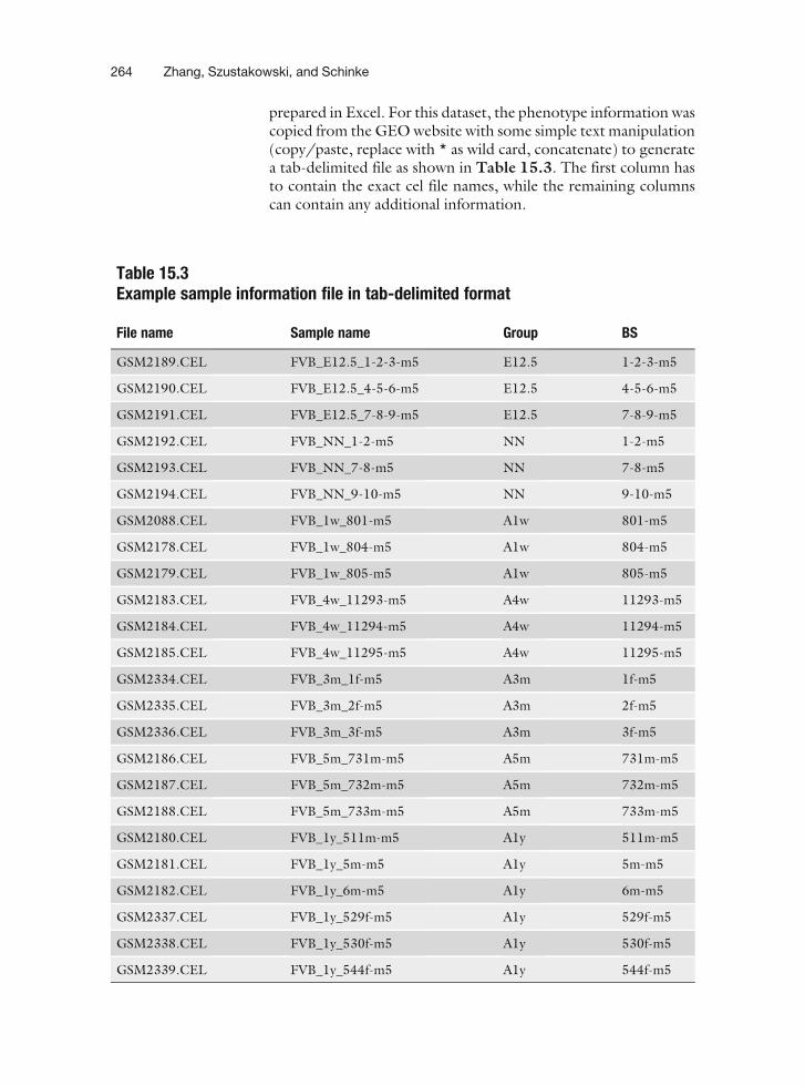
prepared in Excel. For this dataset, the phenotype information wascopied from the GEOwebsite with some simple text manipulation(copy/paste, replace with * as wild card, concatenate) to generatea tab-delimited file as shown in Table 15.3. The first column hasto contain the exact cel file names, while the remaining columnscan contain any additional information.

Table 15.3Example sample information file in tab-delimited format

File name Sample name Group BS

GSM2189.CEL FVB_E12.5_1-2-3-m5 E12.5 1-2-3-m5

GSM2190.CEL FVB_E12.5_4-5-6-m5 E12.5 4-5-6-m5

GSM2191.CEL FVB_E12.5_7-8-9-m5 E12.5 7-8-9-m5

GSM2192.CEL FVB_NN_1-2-m5 NN 1-2-m5



GSM2088.CEL FVB_1w_801-m5 A1w 801-m5

GSM2178.CEL FVB_1w_804-m5 A1w 804-m5

GSM2179.CEL FVB_1w_805-m5 A1w 805-m5

GSM2183.CEL FVB_4w_11293-m5 A4w 11293-m5

GSM2184.CEL FVB_4w_11294-m5 A4w 11294-m5

GSM2185.CEL FVB_4w_11295-m5 A4w 11295-m5

GSM2334.CEL FVB_3m_1f-m5 A3m 1f-m5



GSM2186.CEL FVB_5m_731m-m5 A5m 731m-m5



GSM2180.CEL FVB_1y_511m-m5 A1y 511m-m5



GSM2337.CEL FVB_1y_529f-m5 A1y 529f-m5




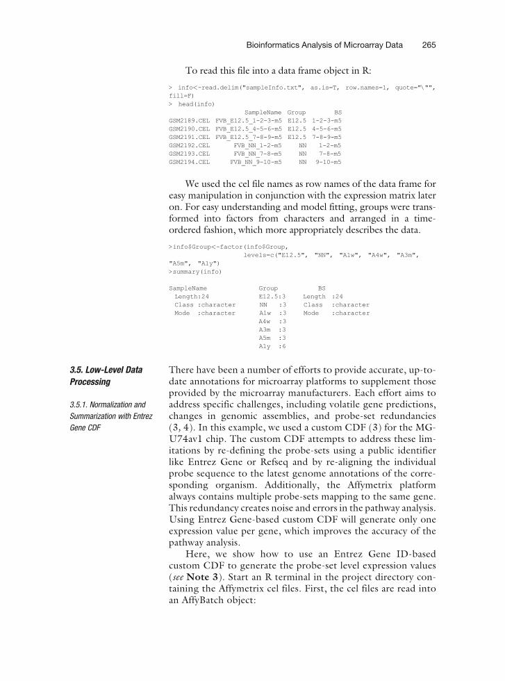
To read this file into a data frame object in R:

> info<-read.delim("sampleInfo.txt", as.is=T, row.names=1, quote="\"",fill=F)> head(info)

SampleName Group BSGSM2189.CEL FVB_E12.5_1-2-3-m5 E12.5 1-2-3-m5GSM2190.CEL FVB_E12.5_4-5-6-m5 E12.5 4-5-6-m5GSM2191.CEL FVB_E12.5_7-8-9-m5 E12.5 7-8-9-m5GSM2192.CEL FVB_NN_1-2-m5 NN 1-2-m5GSM2193.CEL FVB_NN_7-8-m5 NN 7-8-m5GSM2194.CEL FVB_NN_9-10-m5 NN 9-10-m5

We used the cel file names as row names of the data frame foreasy manipulation in conjunction with the expression matrix lateron. For easy understanding and model fitting, groups were trans-formed into factors from characters and arranged in a time-ordered fashion, which more appropriately describes the data.

>info$Group<-factor(info$Group,levels=c("E12.5", "NN", "A1w", "A4w", "A3m",

"A5m", "A1y")>summary(info)

SampleName Group BSLength:24 E12.5:3 Length :24Class :character NN :3 Class :characterMode :character A1w :3 Mode :character

A4w :3A3m :3A5m :3A1y :6

3.5. Low-Level DataProcessing

3.5.1. Normalization and

Summarization with Entrez

Gene CDF

There have been a number of efforts to provide accurate, up-to-date annotations for microarray platforms to supplement thoseprovided by the microarray manufacturers. Each effort aims toaddress specific challenges, including volatile gene predictions,changes in genomic assemblies, and probe-set redundancies(3, 4). In this example, we used a custom CDF (3) for the MG-U74av1 chip. The custom CDF attempts to address these lim-itations by re-defining the probe-sets using a public identifierlike Entrez Gene or Refseq and by re-aligning the individualprobe sequence to the latest genome annotations of the corre-sponding organism. Additionally, the Affymetrix platformalways contains multiple probe-sets mapping to the same gene.This redundancy creates noise and errors in the pathway analysis.Using Entrez Gene-based custom CDF will generate only oneexpression value per gene, which improves the accuracy of thepathway analysis.

Here, we show how to use an Entrez Gene ID-basedcustom CDF to generate the probe-set level expression values(see Note 3). Start an R terminal in the project directory con-taining the Affymetrix cel files. First, the cel files are read intoan AffyBatch object:


>library(affy)>batch<-ReadAffy(celfile.path="cel")>cdfName(batch)[1 ] "MG_U74A"

Changing the CDF name of the AffyBatch object to"mm74av1mmentrezg" will enable the data processing usingthe custom CDF file ‘‘mm74av1mmentrezg.’’

>library(mm74av1mmentrezg)>cdfName(batch)<-"mm74av1mmentrezg">save(batch, file="obj/batch.RData")

The probe logarithmic intensity error (PLIER) method withquantile normalization and mismatch correction was used to gen-erate more accurate results (5–7), especially for probe-sets withlow expression. PLIER produces an improved signal (a summaryvalue for a probe set) by accounting for experimentally observedpatterns for feature behavior and handling error at low and highabundances across multiple arrays. For more information, pleasesee the Affymetrix PLIER technical note (5).

>library(plier)>eset<-justPlier(batch, normalize=T)>exp<-exprs(eset)>pairs(exp[,1:3])

The last command generates a pair–pair scatter plot of the firstthree arrays. As shown in Fig. 15.2A, there are some expressionvalues ranging from 0 to 1 with exaggerated variance in log 2 scale.However, it’s common practice to perform statistical analysis on alog-transformed scale.One simple solution is to add a small constant

GSM2088.CEL

GSM2178.CEL

GSM2179.CEL

GSM2088.CEL

GSM2178.CEL

GSM2179.CEL

-10 -5 0 5 10 15 4 6 8 10 12 14

4 6 8 10 12 144 6 8 10 12 14

46

810

1214

46

810

1214

46

810

1214

-10 -5 0 5 10 15 -10 -5 0 5 10 15

-10

-50

510

15

-10

-50

510

15-1

0-5

05

1015

A B

Fig. 15.2. Pair-wise scatter plot of expression values from microarrays 1 to 3 after low-level data processing. (A) Plotbefore flooring with a constant value. Large variance is observed for values between 0 and 1. (B) Data were plotted afterflooring with a constant value.


number to floor the data. This can effectively reduce nuisancevariation after transformation (Fig. 15.2B) with little impact onhighly expressed genes. This method is also recommended in thePLIER technical note (5).

>exp<-log2(2^exp+16)>pairs(exp [,1:3])>save(exp, file="obj/exp.RData")

3.5.2. Gene Filtering

with MAS5 Calls

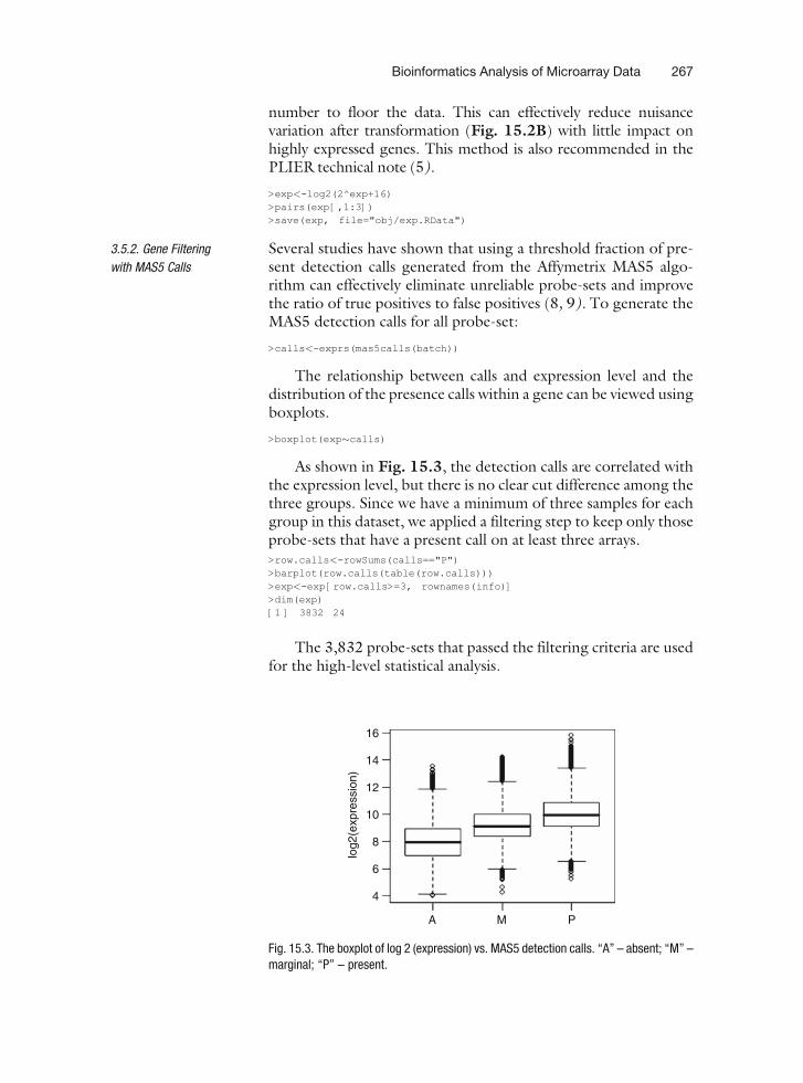
Several studies have shown that using a threshold fraction of pre-sent detection calls generated from the Affymetrix MAS5 algo-rithm can effectively eliminate unreliable probe-sets and improvethe ratio of true positives to false positives (8, 9). To generate theMAS5 detection calls for all probe-set:

>calls<-exprs(mas5calls(batch))

The relationship between calls and expression level and thedistribution of the presence calls within a gene can be viewed usingboxplots.

>boxplot(exp"calls)

As shown in Fig. 15.3, the detection calls are correlated withthe expression level, but there is no clear cut difference among thethree groups. Since we have a minimum of three samples for eachgroup in this dataset, we applied a filtering step to keep only thoseprobe-sets that have a present call on at least three arrays.>row.calls<-rowSums(calls=="P")>barplot(row.calls(table(row.calls)))>exp<-exp[row.calls>=3, rownames(info)]>dim(exp)[1 ] 3832 24

The 3,832 probe-sets that passed the filtering criteria are usedfor the high-level statistical analysis.

16

14

12

10

8

6

4

A M P

log2

(exp

ress

ion)

Fig. 15.3. The boxplot of log 2 (expression) vs. MAS5 detection calls. ‘‘A’’ – absent; ‘‘M’’ –marginal; ‘‘P’’ – present.


3.6. PrincipalComponent Analysis(PCA)

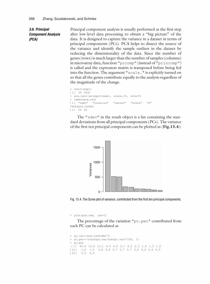
Principal component analysis is usually performed as the first stepafter low-level data processing to obtain a ‘‘big picture’’ of thedata. It is designed to capture the variance in a dataset in terms ofprincipal components (PCs). PCA helps to dissect the source ofthe variance and identify the sample outliers in the dataset byreducing the dimensionality of the data. Since the number ofgenes (rows) is much larger than the number of samples (columns)in microarray data, function "prcomp" (instead of "princomp")is called and the expression matrix is transposed before being fedinto the function. The argument "scale." is explicitly turned onso that all the genes contribute equally to the analysis regardless ofthe magnitude of the change.

> dim(t(exp))[1 ] 24 3832> pca.res<-prcomp(t(exp), scale.=T, retx=T)> names(pca.res)[1 ] "sdev" "rotation" "center" "scale" "x">dim(pca.res$x)[1 ] 24 24

The "sdev" in the result object is a list containing the stan-dard deviations from all principal components (PCs). The varianceof the first ten principal components can be plotted as (Fig.15.4):

> plot(pca.res, las=1)

The percentage of the variation "pc.per" contributed fromeach PC can be calculated as

> pc.var<-pca.res$sdev^2> pc.per<-round(pc.var/sum(pc.var)*100, 1)> pc.per[1 ] 45.0 13.4 13.1 4.3 4.0 2.7 2.5 2.3 1.6 1.3 1.2

[12 ] 1.0 1.0 0.8 0.8 0.7 0.7 0.7 0.6 0.6 0.6 0.5[23 ] 0.5 0.0

1500

1000

500

0

Var

ianc

es

Fig. 15.4. The Scree plot of variance, contributed from the first ten principal components.


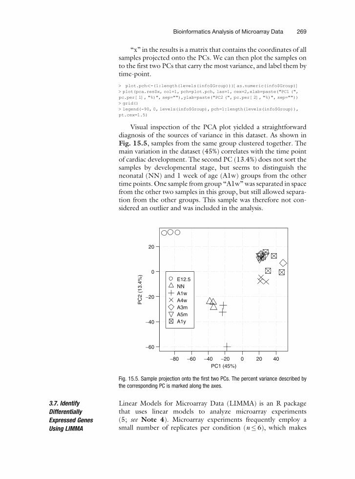
‘‘x’’ in the results is a matrix that contains the coordinates of allsamples projected onto the PCs. We can then plot the samples onto the first two PCs that carry the most variance, and label them bytime-point.

> plot.pch<-(1:length(levels(info$Group)))[as.numeric(info$Group)]> plot(pca.res$x, col=1, pch=plot.pch, las=1, cex=2,xlab=paste("PC1 (",pc.per [1], "%)", sep=""),ylab=paste("PC2 (", pc.per [2], "%)", sep=""))> grid()> legend(-90, 0, levels(info$Group), pch=1:length(levels(info$Group)),pt.cex=1.5)

Visual inspection of the PCA plot yielded a straightforwarddiagnosis of the sources of variance in this dataset. As shown inFig. 15.5, samples from the same group clustered together. Themain variation in the dataset (45%) correlates with the time pointof cardiac development. The second PC (13.4%) does not sort thesamples by developmental stage, but seems to distinguish theneonatal (NN) and 1 week of age (A1w) groups from the othertime points. One sample from group ‘‘A1w’’ was separated in spacefrom the other two samples in this group, but still allowed separa-tion from the other groups. This sample was therefore not con-sidered an outlier and was included in the analysis.

3.7. IdentifyDifferentiallyExpressed GenesUsing LIMMA

Linear Models for Microarray Data (LIMMA) is an R packagethat uses linear models to analyze microarray experiments(5; see Note 4). Microarray experiments frequently employ asmall number of replicates per condition (n#6), which makes

-80 -60 -40 -20 0 20 40

-60

-40

-20

0

20

PC1 (45%)

PC

2 (1

3.4%

)

E12.5NNA1wA4wA3mA5mA1y

Fig. 15.5. Sample projection onto the first two PCs. The percent variance described bythe corresponding PC is marked along the axes.


estimating the variance of a gene’s expression level difficult.Consequently, traditional statistical methods such as the t-testcan be unreliable. LIMMA leverages the large number of observa-tions in a microarray experiment to moderate the variance esti-mates in a data dependent fashion. The output of LIMMA istherefore similar to the output of a t-test but stabilized againstthe effects of small sample sizes. Our purpose was to use thispackage to identify significantly differentially expressed genesacross different time points. To fit the data with the linearmodel, we constructed a design matrix from a ‘‘target’’ vectorwhich contains the grouping information (i.e., the ‘‘Group’’ col-umn in the info data frame in this example).

>library(limma)>levels(info$Group)[1 ] "E12.5" "NN" "1w" "4w" "3m" "5m" "1y"> lev<-levels(info$Group)> design<-model.matrix("0+info$Group)> colnames(design)<-lev> dim(design)[1 ] 24 7> head(design)

E12.5 NN A1w A4w A3m A5m A1y1 1 0 0 0 0 0 02 1 0 0 0 0 0 03 1 0 0 0 0 0 04 0 1 0 0 0 0 05 0 1 0 0 0 0 06 0 1 0 0 0 0 0

To fit the linear model with the design matrix:

> fit<-lmFit(exp, design)> names(fit)[1 ] "coefficients" "rank" "assign" "qr"[5 ] "df.residual" "sigma" "cov.coefficients" "stdev.unscaled"[9 ] "pivot" "genes" "method" "design"

Here, the design matrix is in a group means parameterization,where the coefficients are the mean expression of each group. Tofind the differences among these coefficients, an explicitly definedcontrast matrix is required. For this dataset, we generated all thepair-wise comparisons.

> contr.str<-c()> len<-length(lev)> for(i in 1:(len-1))+ contr.str<-c(contr.str, paste(lev[(i+1):len], lev[i], sep="-"))> contr.str[1 ] "NN-E12.5" "A1w-E12.5" "A4w-E12.5" "A3m-E12.5" "A5m-E12.5" "A1y-E12.5"[7 ] "A1w-NN" "A4w-NN" "A3m-NN" "A5m-NN" "A1y-NN" "A4w-A1w"

[13 ] "A3m-A1w" "A5m-A1w" "A1y-A1w" "A3m-A4w" "A5m-A4w" "A1y-A4w"[19 ] "A5m-A3m" "A1y-A3m" "A1y-A5m"> contr.mat<-makeContrasts(contrasts=contr.str, levels=lev)> fit2<-contrasts.fit(fit, contr.mat)> fit2<-eBayes(fit2)> names(fit2)[1 ] "coefficients" "rank" "assign" "qr"[5 ] "df.residual" "sigma" "cov.coefficients" "stdev.unscaled"


[9 ] "genes" "method" "design" "contrasts"[13 ] "df.prior" "s2.prior" "var.prior" "proportion"[17 ] "s2.post" "t" "p.value" "lods"[21 ] "F" "F.p.value"

Now "coefficients" in the "fit2" contains difference,or log 2 fold change, and "p.value" is the moderated t-test p-value associated with all the pair-wise comparisons. "F" and"F.p.value" is the moderated F-test given for all those compar-isons. The statistics for the changes of all genes across all groupscan be retrieved, sorted by F-test p-values, integrated with geneannotation and output into a tab-delimited file:

> f.top<-topTableF(fit2, number=nrow(exp))> f.top<-cbind(ann [f.top[[1]] 1:4], f.top[,c(2:7, 23:25)])> write.table(f.top, file="f.top.txt", sep="\t", row.names=F, quote=F)> head(f.top)

ProbeSet GeneID Symbol14955_at 14955_at 14955 H1916002_at 16002_at 16002 Igf212797_at 12797_at 12797 Cnn115126_at 15126_at 15126 Hba-x98932_at 98932_at 98932 Myl920250_at 20250_at 20250 Scd2

GeneName14955_at H19 fetal liver mRNA16002_at insulin-like growth factor 212797_at calponin 115126_at hemoglobin X, alpha-like embryonic chain in Hba complex98932_at myosin, light polypeptide 9, regulatory20250_at stearoyl-Coenzyme A desaturase 2

NN.E12.5 A1w.E12.5 A4w.E12.5 A3m.E12.514955_at -0.1262318 -1.368427 -4.639086 -5.98333016002_at -0.2315497 -1.185102 -3.823067 -4.82522112797_at -5.6486004 -5.710477 -6.103997 -6.37526115126_at -4.8768229 -5.507456 -5.037622 -5.26748998932_at -0.4566940 -1.719379 -3.931495 -4.21832320250_at -0.7785607 -1.832313 -3.600636 -3.994683

A5m.E12.5 A1y.E12.5 F P.Value14955_at -5.572897 -5.783935 1087.2210 2.099165e-2516002_at -4.705602 -4.761241 819.2029 4.251770e-2412797_at -6.160193 -6.254116 654.1071 4.635634e-2315126_at -5.100509 -5.210385 567.7905 2.078625e-2298932_at -4.957873 -4.828438 430.2656 3.916275e-2120250_at -3.860944 -4.052382 429.1944 4.020864e-21

adj.P.Val14955_at 8.043999e-2216002_at 8.146390e-2112797_at 5.921249e-2015126_at 1.991323e-1998932_at 2.243523e-1820250_at 2.243523e-18

Themiddle columns (nos. 5–10) of the table contain the log 2fold changes of all other time points vs. embryonic 12.5 d.p.c. Wecan loop through all two-group comparisons and output theresults:

> for(i in 1:ncol(contr.mat)){+ t.top<-topTable(fit2, coef=i, number=nrow(exp))+ t.top<-cbind(ann[t.top[[1]],], t.top[, 2:ncol(t.top)])+ write.table(t.top, sep="\t", row.names=F, quote=F,


+ file=file.path("limma", paste(contr.str[i], "top.txt",sep=".")))+}

3.8. Clustering Analysis Clustering analysis has been widely applied to gene expressiondata for pattern discovery. Hierarchical clustering is a fre-quently used method that does not require the user to specifythe number of clusters a priori (see Note 5). Since all genescontribute equally, genes with no changes between groups onlyadd noise to the clustering. Thus, statistical filters are oftenapplied to eliminate such genes prior to the clustering proce-dure. In our dataset, there were a large number of filteredgenes (2,663, 69.6%) with a statistically significant changeabove a Benjamini–Hochberg (BH) (10) adjusted p-value cut-off of <0.01. Consequently, we further limited the clusteringto those genes that showed at least a twofold differencebetween any two of the seven time-points.

> g.2f<-(rowSums(abs(fit2[[1]][rownames(exp),])>1)>0) &+ (f.top[rownames(exp),]$adj.P.Val<0.01)> sum(g.2f)[1 ] 1680

A total of 1,680 genes passed this criteria. The gene expressionmatrix was standardized before calculating the Euclidean distancesbetween the genes.

> exp.std<-sweep(exp, 1, rowMeans(exp))> row.sd<-apply(exp, 1, sd)> exp.std<-sweep(exp.std, 1, row.sd, "/")> save(exp.std, file="obj/exp.std.RData")> exp.cl<-exp.std[g.2f,]

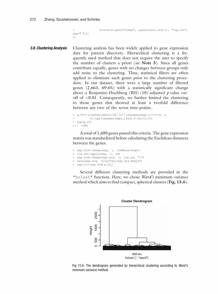
Several different clustering methods are provided in the"hclust" function. Here, we chose Ward’s minimum variancemethodwhich aims to find compact, spherical clusters (Fig. 15.6).

2500

1500

500

0

Hei

ght

Cluster Dendrogram

dist.euhclust (*, “ward”)

Fig 15.6. The dendrogram generated by hierarchical clustering according to Ward’sminimum variance method.


> hc.res<-hclust(dist.eu, method="ward")> plot(hc.res, labels=F)

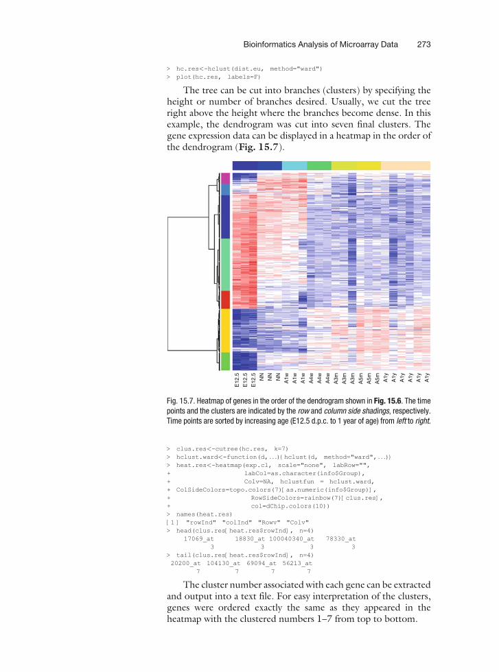
The tree can be cut into branches (clusters) by specifying theheight or number of branches desired. Usually, we cut the treeright above the height where the branches become dense. In thisexample, the dendrogram was cut into seven final clusters. Thegene expression data can be displayed in a heatmap in the order ofthe dendrogram (Fig. 15.7).

> clus.res<-cutree(hc.res, k=7)> hclust.ward<-function(d, . . .){hclust(d, method="ward", . . .)}> heat.res<-heatmap(exp.cl, scale="none", labRow="",+ labCol=as.character(info$Group),+ Colv=NA, hclustfun = hclust.ward,+ ColSideColors=topo.colors(7)[as.numeric(info$Group)],+ RowSideColors=rainbow(7)[clus.res],+ col=dChip.colors(10))> names(heat.res)[1 ] "rowInd" "colInd" "Rowv" "Colv"> head(clus.res[heat.res$rowInd], n=4)

17069_at 18830_at 100040340_at 78330_at3 3 3 3

> tail(clus.res[heat.res$rowInd], n=4)20200_at 104130_at 69094_at 56213_at

7 7 7 7

The cluster number associated with each gene can be extractedand output into a text file. For easy interpretation of the clusters,genes were ordered exactly the same as they appeared in theheatmap with the clustered numbers 1–7 from top to bottom.

E12

.5E

12.5

E12

.5N

NN

NN

NA

1wA

1wA

1wA

4wA

4wA

4wA

3mA

3mA

3mA

5mA

5mA

5m A1y

A1y

A1y

A1y

A1y

A1y

Fig. 15.7. Heatmap of genes in the order of the dendrogram shown in Fig. 15.6. The timepoints and the clusters are indicated by the row and column side shadings, respectively.Time points are sorted by increasing age (E12.5 d.p.c. to 1 year of age) from left to right.


> clus.order<-unique(clus.res[heat.res$rowInd])> clus.order ##this is from bottom to top in the heatmap[1 ] 3 2 1 4 6 5 7> gene.clus.order<-match(clus.res[heat.res$rowInd], clus.order)> names(gene.clus.order)<-names(clus.res[heat.res$rowInd])> head(gene.clus.order)17069_at 18830_at 100040340_at 78330_at 101540_at 18032_at

1 1 1 1 1 1> gene.clus.order<-rev(gene.clus.order)> gene.clus.order<-max(gene.clus.order)-gene.clus.order+1> clus.ann<-ann[names(gene.clus.order),]> clus.ann$cluster<-gene.clus.order> head(clus.ann[,c(2:3,5)])

GeneID Symbol cluster56213_at 56213 Htra1 169094_at 69094 Tmem160 1104130_at 104130 Ndufb11 120200_at 20200 S100a6 126968_at 26968 Islr 181877_at 81877 Tnxb 1> write.table(clus.ann, file="clus.ann.txt", sep="\t", row.names=F,na="")

The functional enrichment for each cluster can be calculatedusing the ‘‘GOstats’’ package from Bioconductor, or using theweb-tool DAVID (Database for Annotation, Visualization, andIntegrated Discovery, http://david.abcc.ncifcrf.gov (11).

3.9. Pathway (Gene-Set) Analysis

Gene-set analysis is especially helpful for identifying the biologicalthemes related to changes between two conditions or for correla-tion with a specific numeric phenotypical measurement. FollowingMootha’s Gene-Set Enrichment Analysis (GSEA), Tian et al. (12)proposed to rank gene-sets based on two statistics,NTk andNEk,and estimate q-values for each pathway or gene-set to address twodifferent aspects in pathway analysis. Given a gene-set g, NTkcomputes whether g is significantly changed compared to allother gene-sets. NEk serves as an indicator of whether the geneswithin g as a whole group are significantly correlated with thephenotype. ‘‘sigPathway’’ is an R package implementation of themethod (see Note 6). Here, we show how to use sigPathway inorder to identify pathways that are statistically significantly differ-ent between two developmental stages, NN and E12.5 d.p.c.

3.9.1. Construct Gene-Sets

Object for sigPathway

First, we constructed an R list object that contains the gene-setannotation list we would like to use for the calculations. sigPath-way will calculate the composite statistics NTk and NEk for eachgene-set within this list. If the annotation list is named G, eachelement of G is an R list object representing one gene list andshould include three essential elements:1. source: the source of gene-set, e.g., GO, BP, or KEGG;

2. title: the title for the gene-set, e.g., ‘‘ABC transporters’’;

3. probes: a unique set of probe(-set)s that belong to thegene-set.


The annotation list can be from any source, including user-defined lists. Gene Ontology (GO) annotation is usually consid-ered the most inclusive and fastest-growing public source forgrouping functionally relevant genes. The following procedureshows how to build an up-to-date gene-set annotation list fromscratch, starting with the "org.Mm.egGO2ALLEGS" and "GO"packages from Bioconductor.

First, a list of GO terms to Entrez Gene IDmapping is created.

> library(sigPathway)> library(GO)> x<-as.list(org.Mm.egGO2ALLEGS)> length(x)[1 ] 7938> head(names(x))[1 ] "GO:0008150" "GO:0008152" "GO:0006464" "GO:0006468" "GO:0006793"[6 ] "GO:0006796"> len<-unlist(lapply(x, length))> head(len)GO:0008150 GO:0008152 GO:0006464 GO:0006468 GO:0006793 GO:0006796

21965 8832 1505 650 870 870

To exclude genes that are not included in this CDF(mm74av1mmentrezg):

> x<-lapply(x, function(y, all.gene.id){+ y<-y[y %in% all.gene.id]+ unique(y)+ }, unique(ann$GeneID))> len<-unlist(lapply(x, length))> summary(len)

Min. 1st Qu. Median Mean 3rd Qu. Max.0.00 1.00 2.00 32.82 8.00 5853.00

The number of genes in a gene-set ranges from 0 to 5,853genes, but we usually limit our analysis to include gene-sets withabout 5–500 genes. If there are too few genes in the gene-sets, theresults could be driven by only one or two genes with largeexpression changes and not fairly reflect the whole pathway. Onthe other hand, it can be difficult to interpret the biological mean-ing when the number of genes in a gene-set is too large.

> lo<-5> hi<-500> x<-x[len>=lo & len<=hi]> length(x)[1 ] 3452

The list "x" contains the probe-sets for 3,452 GO IDs. Thetitles and definitions for the GO terms can be obtained using theGO package:> library(GO)> gt<-as.list(GOTERM)> length(gt)[1 ] 23679> gt[1:2]$‘GO:0019980‘GOID: GO:0019980Term: interleukin-5 binding


Ontology: MFDefinition: Interacting selectively with interleukin-5.Synonym: IL-5 binding

$‘GO:0004213‘

GOID: GO:0004213

Term: cathepsin B activity

Ontology: MF

Definition: Catalysis of the hydrolysis of peptide bonds with a broadspecificity. Preferentially cleaves the terminal bond of -Arg-Arg-Xaa motifs in small molecule substrates (thusdiffering from cathepsin L). In addition to being anendopeptidase shows peptidyl-dipeptidase activityliberating C-terminal dipeptides.

To generate the gene-set annotation list G:

> G<-list()> for(i in names(x)){+ G[[i]]<-list()+ G[[i]]$src<-gt[[i]]@Ontology+ G[[i]]$name<-paste(i, gt[[i]]@Term)+ G[[i]]$probes<-paste(x[[i]], "at", sep="_")+ }> save(G, file="G.RData")> length(G)[1 ] 2708> head(names(G))[1 ] "GO:0006468" "GO:0006793" "GO:0006796" "GO:0006915" "GO:0008219"[6 ] "GO:0012501"> class(G)[1 ] "list"> class(G[[1]])[1 ] "list"> names(G[[1]])[1 ] "src" "title" "probes"> G[[1]][1:2]$src[1 ] "BP"

$title

[1 ] "GO:0006468 protein amino acid phosphorylation"

This list "G" is saved and can be used later for any datasetpre-processed with the CDF mm74mmav1entrezg. For thisanalysis, we restricted the gene-sets to those with 5–200 probe-sets that are present in the filtered expression data by using the"selectGeneSets" function. The list that was used is recordedin list "g" without altering the annotation list object "G."

> exp<-exp[-c(grep("AFFX", rownames(exp))),]> g<-selectGeneSets(G, rownames(exp), minNPS=5, maxNPS=200)> names(g)[1 ] "nprobesV" "indexV" "indGused"> length(g[[1]])[1 ] 1652

Gene-sets (1,652) were used in the analysis after this filter. Thenext step was to construct the expression data matrix for compar-ing the neonatal stage ‘‘NN’’ vs. embryonic stage ‘‘E12.5’’ andcalculate the NTk and NEk statistics.


> samples.ref<-rownames(info)[info$Group=="E12.5"]> exp.ref<-exp[, samples.ref]> samples.test<-rownames(info)[info$Group=="NN"]> exp.test<-exp[, samples.test]> phenotype<-rep(c(0, 1), c(length(samples.ref), length(samples.test)))> tab<-cbind(exp.ref, exp.test)> NTk<-calculate.NTk(tab, phenotype, g)> NEk<-calculate.NEk(tab, phenotype, g)’nsim’ is greater than the number of unique permutationsChanging ’nsim’ to 19, excluding the unpermuted case

To view the NEk/NTk distributions and their relationship:

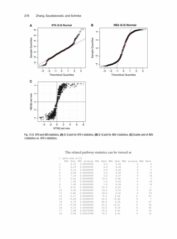
> par(mfrow=c(2,2), mex=0.7, ps=9)> qqnorm(NTk$t.set.new, main="NTk Q-Q Normal")> qqline(NTk$t.set.new, col=2)> qqnorm(NEk$t.set.new, main="NEk Q-Q Normal")> qqline(NEk$t.set.new, col=2)> plot(NTk$t.set.new, NEk$t.set.new, cex=0.7)> abline(h=0)> abline(v=0)> grid()

As shown in Fig. 15.8A and B, both the NEk and NTkstatistics are symmetrically distributed, but NTk has a longer‘‘tail’’ and NEk a shorter ‘‘tail’’ than a normal distribution. Thetwo statistics are positively correlated. By default, the top 25enriched gene-sets ranked by averaging the individual ranks ofboth, NTk and NEk rankings, can be retrieved as> path.res<-rankPathways(NTk, NEk, G, tab, phenotype, g, ngroups=2,+ methodNames=c("NTk", "NEk"), allpathways=T)> names(path.res)[1 ] "IndexG" "Gene Set Category" "Pathway"[4 ] "Set Size" "Percent Up" "NTk Stat"[7 ] "NTk q-value" "NTk Rank" "NEk Stat"

[10 ] "NEk q-value" "NEk Rank"> path.res$Pathway[1 ] "GO:0006817 phosphate transport"[2 ] "GO:0005581 collagen"[3 ] "GO:0030020 extracellular matrix structural constituent conferring

tensile strength"[4 ] "GO:0005201 extracellular matrix structural constituent"[5 ] "GO:0044420 extracellular matrix part"[6 ] "GO:0005605 basal lamina"[7 ] "GO:0005578 proteinaceous extracellular matrix"[8 ] "GO:0031012 extracellular matrix"[9 ] "GO:0004364 glutathione transferase activity"

[10 ] "GO:0015698 inorganic anion transport"[11 ] "GO:0006820 anion transport"[12 ] "GO:0006084 acetyl-CoA metabolic process"[13 ] "GO:0006270 DNA replication initiation"[14 ] "GO:0005604 basement membrane"[15 ] "GO:0008094 DNA-dependent ATPase activity"[16 ] "GO:0006631 fatty acid metabolic process"[17 ] "GO:0006638 neutral lipid metabolic process"[18 ] "GO:0006639 acylglycerol metabolic process"[19 ] "GO:0006099 tricarboxylic acid cycle"[20 ] "GO:0009060 aerobic respiration"[21 ] "GO:0009109 coenzyme catabolic process"[22 ] "GO:0046356 acetyl-CoA catabolic process"[23 ] "GO:0051187 cofactor catabolic process"[24 ] "GO:0044445 cytosolic part"[25 ] "GO:0032787 monocarboxylic acid metabolic process"


The related pathway statistics can be viewed as

> path.res[,6:11]NTk Stat NTk q-value NTk Rank NEk Stat NEk q-value NEk Rank

1 6.33 0.00000000 4.0 4.43 0 62 6.14 0.00000000 6.0 4.44 0 53 6.14 0.00000000 6.0 4.44 0 54 6.89 0.00000000 3.0 4.40 0 125 7.19 0.00000000 2.0 4.37 0 146 5.22 0.00000000 13.0 4.46 0 37 7.92 0.00000000 1.0 4.36 0 198 7.92 0.00000000 1.0 4.36 0 199 4.41 0.00000000 31.0 4.53 0 110 5.02 0.00000000 15.0 4.33 0 2111 4.80 0.00000000 22.0 4.32 0 2312 6.17 0.00000000 5.0 4.26 0 4313 -3.09 0.03690476 51.5 -4.42 0 714 4.74 0.00000000 24.0 4.29 0 3715 -3.69 0.00000000 41.0 -4.31 0 3016 5.13 0.00000000 14.0 4.16 0 6517 2.88 0.05470588 72.0 4.41 0 1018 2.88 0.05470588 72.0 4.41 0 10

-3 -2 -1 0 1 2 3

-4-2

02

46

8

NTk Q-Q Normal

Theoretical Quantiles

Sam

ple

Qua

ntile

s

-3 -2 -1 0 1 2 3

-4-2

02

4

NEk Q-Q Normal

Theoretical Quantiles

Sam

ple

Qua

ntile

s

-4 -2 0 2 4 6 8

-4-2

02

4

NTk$t.set.new

NE

k$t.s

et.n

ew

A B

C

Fig. 15.8. NTk and NEk statistics. (A) Q–Q plot for NTk t-statistics. (B) Q–Q plot for NEk t-statistics. (C) Scatter plot of NEkt-statistics vs. NTk t-statistics.


19 4.92 0.00000000 20.0 4.16 0 6420 4.92 0.00000000 20.0 4.16 0 6421 4.92 0.00000000 20.0 4.16 0 6422 4.92 0.00000000 20.0 4.16 0 6423 4.85 0.00000000 21.0 4.17 0 6324 -3.09 0.03690476 51.5 -4.29 0 3325 5.27 0.00000000 12.0 4.14 0 73

The extracellular matrix (ECM) and fatty acid metabolismgene-sets were the most up-regulated and DNA replication/cell cycle gene-sets were most down-regulated whencomparing NN vs. E12.5 d.p.c. developmental stages. Thegene-sets with the highest NTk rank is "GO:0031012extracellular matrix." The NTk t-statistic of 7.92was much higher than the second ranked gene-set"GO:0006817 phosphate transport" (NTk 6.33), how-ever, the NEk t-statistics of the two gene-sets were about thesame. This scenario is clearly displayed in Fig. 15.8C, inwhich the tails of the NTk t-statistics spread wider than thetails of the NEk t-statistics Thus, it is more meaningful to rankthe significance of the gene-sets based on the mean of NEkand NTk t-statistics rather than based on the average rankingof the two, which is the default. This can be done by specify-ing the argument "npath" in "rankPathways" function tothe number of total gene-sets, and then reordering the dataframe:

> path.res<-rankPathways(NTk, NEk, G, tab, phenotype, g, ngroups=2,+ methodNames=c("NTk", "NEk"), npath=NTk$ngs)> ave.stat<-rowMeans(path.res[,c(6,9)])> path.res<-path.res[order(abs(ave.stat), decreasing=T),]> head(path.res[[3]])[1 ] "GO:0005578 proteinaceous extracellular matrix"[2 ] "GO:0031012 extracellular matrix"[3 ] "GO:0044420 extracellular matrix part"[4 ] "GO:0005201 extracellular matrix structural constituent"[5 ] "GO:0006817 phosphate transport"[6 ] "GO:0005581 collagen"

Finally, it is of interest to view the genes that contributed tothe changes, especially for those top-ranked gene-sets. For exam-ple, we retrieved the statistics for all the genes in gene-set‘‘GO:0006817 phosphate transport,’’ which is ranked on fifthplace on the "path.res" list.

> t.stat<-calcTStatFast(tab, phenotype, ngroups=2)> path.stat<-getPathwayStatistics(tab, phenotype, G, path.res$IndexG,+ statList=t.stat)> st1<-path.stat[[5]]> head(st1)

Probes Mean_0 Mean_1 StDev_0 StDev_11 11487_at 9.560018 8.922373 0.18504668 0.153794362 11490_at 9.925778 10.564280 0.12777095 0.186934173 11492_at 9.407763 10.108199 0.09667248 0.242422134 11603_at 11.535603 11.362591 0.17646941 0.063228085 12111_at 10.942530 12.093049 0.23738825 0.137032606 12159_at 11.454837 9.619270 0.27848105 0.08053406


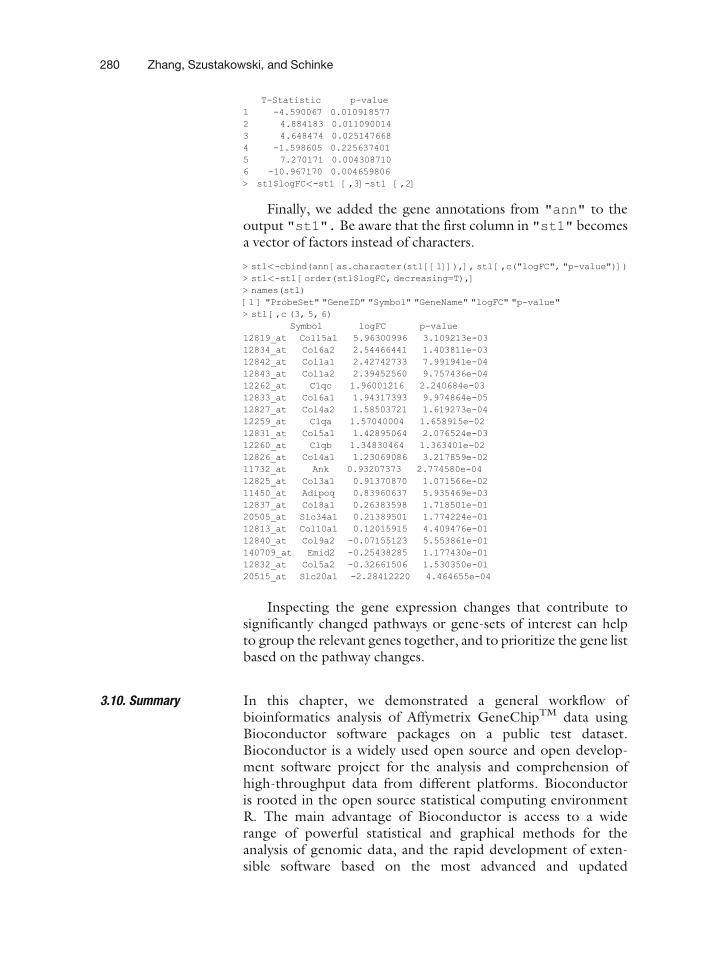
T-Statistic p-value1 -4.590067 0.0109185772 4.884183 0.0110900143 4.648474 0.0251476684 -1.598605 0.2256374015 7.270171 0.0043087106 -10.967170 0.004659806> st1$logFC<-st1 [,3]-st1 [,2]

Finally, we added the gene annotations from "ann" to theoutput "st1". Be aware that the first column in "st1" becomesa vector of factors instead of characters.

> st1<-cbind(ann [as.character(st1 [[1]]),], st1 [,c("logFC", "p-value")])> st1<-st1 [order(st1$logFC, decreasing=T),]> names(st1)[1 ] "ProbeSet" "GeneID" "Symbol" "GeneName" "logFC" "p-value"> st1 [,c (3, 5, 6)

Symbol logFC p-value12819_at Col15a1 5.96300996 3.109213e-0312834_at Col6a2 2.54466441 1.403811e-0312842_at Col1a1 2.42742733 7.991941e-0412843_at Col1a2 2.39452560 9.757436e-0412262_at C1qc 1.96001216 2.240684e-0312833_at Col6a1 1.94317393 9.974864e-0512827_at Col4a2 1.58503721 1.619273e-0412259_at C1qa 1.57040004 1.658915e-0212831_at Col5a1 1.42895064 2.076524e-0312260_at C1qb 1.34830464 1.363401e-0212826_at Col4a1 1.23069086 3.217859e-0211732_at Ank 0.93207373 2.774580e-0412825_at Col3a1 0.91370870 1.071566e-0211450_at Adipoq 0.83960637 5.935469e-0312837_at Col8a1 0.26383598 1.718501e-0120505_at Slc34a1 0.21389501 1.774224e-0112813_at Col10a1 0.12015915 4.409476e-0112840_at Col9a2 -0.07155123 5.553861e-01140709_at Emid2 -0.25438285 1.177430e-0112832_at Col5a2 -0.32661506 1.530350e-0120515_at Slc20a1 -2.28412220 4.464655e-04

Inspecting the gene expression changes that contribute tosignificantly changed pathways or gene-sets of interest can helpto group the relevant genes together, and to prioritize the gene listbased on the pathway changes.

3.10. Summary In this chapter, we demonstrated a general workflow ofbioinformatics analysis of Affymetrix GeneChipTM data usingBioconductor software packages on a public test dataset.Bioconductor is a widely used open source and open develop-ment software project for the analysis and comprehension ofhigh-throughput data from different platforms. Bioconductoris rooted in the open source statistical computing environmentR. The main advantage of Bioconductor is access to a widerange of powerful statistical and graphical methods for theanalysis of genomic data, and the rapid development of exten-sible software based on the most advanced and updated


analysis algorithms. For users not familiar with R, other soft-ware tools are available to execute the diverse analysis steps, assummarized in Note 7.

We focused our analysis on commonly used strategies fornormalization, probe-set summarization, gene filtering, statisticalanalysis, and pathway prediction. However, many other analysisoptions can be used for each step and have been extensively dis-cussed (6, 13, 14). A list of the available options can also be foundunder the Bioconductor Task View.

Additional high-level data analyses that allow a more in-depthunderstanding of the biology underlying gene expression changesinclude motif analysis for co-expressed genes (15) and gene net-work/topology analysis (16, 17). However, a detailed descriptionof these analyses is beyond the scope of this introductory chapter.

4. Notes

1. R and Bioconductor package installationR installs and updates its packages using an HTTP proto-

col. When installed behind a firewall, an http proxy environ-ment variable must be first set to enable access to the Internetfrom within R.> Sys.setenv(‘‘http_proxy’’ = ‘‘http://my.proxy.net:9999’’;).

2. Additional packages can also be installed from the R terminalmenu ‘‘Packages’’ ! ‘‘select the CRAN mirror’’ ! ‘‘selectrepositories.’’

3. Low-level Affymetrix data processing

Numerousmethods have been published for normalizationand summarization of the probe-level data. The RobustMulti-chip Average (RMA) (18), GC-RMA (19) and MBEI(24) are popular methods. ‘‘LIMMA’’ package also provides aGUI which requires minimal R programming.

4. Statistical Analysis of differentially expressed genes

Other methods for finding differentially expressed genescan be found on the Bioconductor website using ‘‘Task View’’of ‘‘DifferentialExpression’’ under the download section forthe specific release.

5. Clustering using the HOPACH method

Beyond classical hierarchical clustering, the ‘‘HierarchicalOrdered Partitioning and Collapsing Hybrid’’ (HOPACH)package uses the Mean/Median Split Silhouette (MSS) cri-teria to identify the level of the tree with maximally homo-geneous clusters (20). In this case users do not have to


pre-specify the number of clusters. This method usually iden-tifies a larger number of homogeneous cluster with smallersize using the default setting.

6. Gene-SetEnrichmentAnalysis (GSEA)using sigPathwaypackagea. The significance of the results depends on the collection of

gene-sets available. It is important that the pathways exam-ined are relevant to the study.

b. Other pathways like KEGG can be constructed in thesimilar manner as the GO packages. The package alsoprovides functions to import gene-sets in other formats.It is recommended to calculate the pathway statistics sepa-rately for each source due to the redundancy among gene-sets from different sources.

c. The function "writeSigPathway" in the sigPathwaypackage outputs all gene-sets in html format. This functionrequires the chip annotation package with accessionnumbers, which"org.Mm.eg.db"does not provide.How-ever, for datasets summarized with Affymetrix CDF, this is anice utility to view the results in a more user-friendly format.

7. Other statistical software for microarray data analysisThere are many other commercial data analysis packages

and open software available for microarray data analysis forusers not familiar with R programming. Some of the popularpackages and tools include the following:l Complete Analysis (normalization, group comparison,

clustering, etc.)

l GenePattern (21) (Broad Institute)

l geWorkbench (NCI)

http://wiki.c2b2.columbia.edu/workbench/index.php/Home

l GeneSpring from Agilent Technologies

l TM4 (22) – http://www.tm4.org/

l dChip (23, 24)http://biosun1.harvard.edu/complab/dchip/

l Differentially expressed genes

l SAM (25) – http://www-stat.stanford.edu/%7Etibs/SAM/index.html

l PaGE (26) – http://www.cbil.upenn.edu/PaGE/l Pathway/gene-set analysis

l GSEA-P (27, 28):

http://www.broad.mit.edu/gsea/

l GeneTrail (29)

http://genetrail.bioinf.uni-sb.de/


l Ingenuity Pathway Analysis Tool – http://www.ingenuity.com/

l MetaCore – http://www.genego.com

l GenMaPP (30) – http://www.genmapp.org/

l Collection of GO Analysis Tools:http://www.geneontology.org/GO.tools.microarray.shtml

References

1. Reimers,M,Carey, VJ. (2006). Bioconductor:an open source framework for bioinformaticsand computational biology. Method Enzymol411, 119–134.

2. Team, RDC. (2007). R: A language andenvironment for statistical computing.R Foundation for Statistical Computing,Vienna, Austria.

3. Dai, M, Wang, P, Boyd, AD, et al. (2005).Evolving gene/transcript definitions signifi-cantly alter the interpretation of GeneChipdata. Nucleic Acids Res 33, e175.

4. Liu, H, Zeeberg, BR, Qu, G, et al. (2007).AffyProbeMiner: a web resource for com-puting or retrieving accurately redefinedAffymetrix probe sets. Bioinformatics 23,2385–2390.

5. Hubbell, E, Liu,WM,Mei, R.Guide to ProbeLogarithmic Intensity Error (PLIER) Estima-tion. http://www.affymetrix.com/support/technical/technotes/plier_techno te.pdf

6. Choe, SE, Boutros, M, Michelson, AM.(2005). Preferred analysis methods for Affy-metrix GeneChips revealed by a whollydefined control dataset. Genome Biol 6, R16.

7. Seo, J, Hoffman, EP. (2006). Probeset algorithms: is there a rational best bet?BMC Bioinformatics 7, 395.

8. McClintick, JN, Edenberg, HJ. (2006).Effects of filtering by Present call on analysisof microarray experiments. BMC Bioinfor-matics 7, 49.

9. Pepper, SD, Saunders, EK, Edwards, LE,et al. (2007). The utility of MAS5 expres-sion summary and detection call algorithms.BMC Bioinformatics 8, 273.

10. Benjamini, Y, Hochberg, Y. (1995). Con-trolling the false discovery rate: a practicaland powerful approach to multiple testing.J R Stat Soc Series 57, 289–300.

11. Dennis, G, Jr., Sherman, BT, Hosack, J,et al. (2003). DAVID: database for

Annotation, Visualization, and IntegratedDiscovery. Genome Biol 4, P3.

12. Tian, L, Greenberg, SA, Kong, SW, et al.(2005). Discovering statistically significantpathways in expression profiling studies. ProcNatl Acad Sci USA 102, 13544–13549.

13. Nam, D, Kim, SY. (2008). Gene-setapproach for expression pattern analysis.Brief Bioinform 9, 189–197.

14. Raghavan, N, De Bondt, AM, Talloen, W,et al. (2007). The high-level similarity ofsome disparate gene expression measures.Bioinformatics 23, 3032–3038.

15. Mootha, VK, Handschin, C, Arlow, D, et al.(2004). Erralpha and Gabpa/b specifyPGC-1alpha-dependent oxidative phos-phorylation gene expression that is alteredin diabetic muscle. Proc Natl Acad Sci USA101, 6570–6575.

16. Baitaluk, M, Qian, X, Godbole, S, et al.(2006). PathSys: integrating molecularinteraction graphs for systems biology.BMC Bioinformatics 7, 55.

17. Draghici, S, Khatri, P, Tarca, AL, et al.(2007). A systems biology approach forpathway level analysis. Genome Res 17,1537–1545.

18. Irizarry, RA, Bolstad, BM, Collin, F, et al.(2003). Summaries of Affymetrix GeneChipprobe level data. Nucleic Acids Res 31, e15.

19. Wu, Z, Irizarry, RA. (2005). Stochasticmodels inspired by hybridization theory forshort oligonucleotide arrays. J Comput Biol12, 882–893.

20. van der Laan, M, Dudoit, S, Pollard, K.(2003). Hybrid clustering of gene expres-sion data with visualization and bootstrap.J Stat Plan Inference 117,275–303.

21. Reich, M, Liefeld, T, Gould, J, et al. (2006).GenePattern 2.0. Nat Genet 38, 500–501.

22. Saeed, AI, Sharov, V, White, J, et al. (2003).TM4: a free, open-source system for


microarray data management and analysis.Biotechniques 34,374–378.

23. Li, C, Wong, WH. (2001). Model-basedanalysis of oligonucleotide arrays: modelvalidation, design issues and standard errorapplication. Genome Biol 2(8),0032.1–0032.11.

24. Li, C, Wong, WH. (2001). Model-basedanalysis of oligonucleotide arrays: expres-sion index computation and outlier detec-tion. Proc Natl Acad Sci USA 98, 31–36.

25. Tusher, VG, Tibshirani, R, Chu, G. (2001).Significance analysis of microarrays appliedto the ionizing radiation response. ProcNatlAcad Sci USA 98, 5116–5121.

26. Manduchi, E, Grant, GR, McKenzie, SE,et al. (2000). Generation of patterns fromgene expression data by assigning confi-dence to differentially expressed genes.Bioinformatics 16, 685–698.

27. Mootha, VK, Lindgren, CM, Eriksson, KF,et al. (2003). PGC-1alpha-responsive genesinvolved in oxidative phosphorylation are

coordinately downregulated in human dia-betes. Nat Genet 34, 267–273.

28. Subramanian, A, Kuehn, H, Gould, J, et al.(2007). GSEA-P: a desktop application forGene Set Enrichment Analysis. Bioinfor-matics 23, 3251–3253.

29. Backes, C, Keller, A, Kuentzer, J, et al.(2007). GeneTrail–advanced gene setenrichment analysis. Nucleic Acids Res 35,W186–192.

30. Dahlquist, KD, Salomonis, N, Vranizan, K,et al. (2002). GenMAPP, a new tool forviewing and analyzing microarray data onbiological pathways. Nat Genet 31, 19–20.

31. Gautier, L, Cope, L, Bolstad, BM, et al.(2004). Affy–analysis of Affymetrix Gene-Chip data at the probe level. Bioinformatics20, 307–315.

32. Smyth, GK (2004). Linear models andempirical bayes methods for assessing dif-ferential expression in microarray experi-ments. Stat Appl Genet Mol Biol 3(1),Article 3.


chapter 15mpfrende/ecological genomics... · chapter 15 bioinformatics ... dedicated team of...

Documents