chapter 1_dsp1_co thuc_full_bkdn
DESCRIPTION
good job! how do you get itTRANSCRIPT

CHAPTER 1:
INTRODUCTION
Lesson #1: A big picture about Digital Signal Processing
Lesson #2: Analog-to-Digital and Digital-to-Analog
conversion
Lesson #3: The concept of frequency in CT & DT signals
Duration: 5 hrs

Lecture #1: A big picture about
Digital Signal Processing
Duration: 1 hr
Outline:
1. Signals
2. Digital Signal Processing (DSP)
3. Why DSP?
4. DSP applications
Learning Digital Signal Processing is not something you accomplish; it’s a journey you take.
R.G. Lyons, Understanding Digital Signal Processing
* * * * * * *

Signals
Function of independent variables such as time, distance,
position, temperature
Convey information
Examples:
1D signal: speech, music, biosensor…
2D signal: image
2.5D signal: video (2D image + time)
3D signal: animated


2-D image signals
Binary image??? Color image Grey image
(indexed image)

2.5-D video signals

3-D animated signals

Lecture #1: A big picture about
Digital Signal Processing
Duration: 1 hr
Outline:
1. Signals
2. Digital Signal Processing (DSP)
3. Why DSP?
4. DSP applications

What is Digital Signal Processing?
Represent a signal by a sequence of numbers (called a
"discrete-time signal‖ or "digital signal").
Modify this sequence of numbers by a computing process
to change or extract information from the original signal
The "computing process" is a system that converts one
digital signal into another— it is a "discrete-time system‖ or
"digital system―.
Transforms are tools using in computing process

Discrete-time signal vs.
continuous-time signal
Continuous-time signal:
- define for a continuous duration of time
- sound, voice…
Discrete-time signal:
- define only for discrete points in time (hourly, every second, …)
- an image in computer, a MP3 music file
- amplitude could be discrete or continuous
- if the amplitude is also discrete, the signal is digital.

Analog signal vs. digital signal
Analog signal Digital signal
00 10 00 10 11

Signal processing systems
Processing A/D D/A
Analog signal
x(t)
Analog signal
y(t)
Digital signal processing
Processing Analog signal
x(t)
Analog signal
y(t)
Analog signal processing

Digital Signal Processing
implementation
Performed by:
Special-purpose (custom) chips: application-specific integrated
circuits (ASIC)
Field-programmable gate arrays (FPGA)
General-purpose microprocessors or microcontrollers (μP/μC)
General-purpose digital signal processors (DSP processors)
DSP processors with application-specific hardware (HW)
accelerators

Digital Signal Processing
implementation

Digital Signal Processing
implementation
Use basic operations of addition,
multiplication and delay
Combine these operations to accomplish
processing: a discrete-time input signal
another discrete-time output signal

An example of main step:
“DT signal processing”
From a discrete-time input signal:
1 2 4 -9 5 3
Create a discrete-time output signal:
1/3 1 7/3 -1 0 -1/3 8/3 1
What is the relation between input and output signal?

Two main categories of DSP
Analysis Filtering
Measurement Digital Signals
- feature extraction
- signal recognition
- signal modeling
........
- noise removal
- interference
removal
……
Digital Signals

Lecture #1: A big picture about
Digital Signal Processing
Duration: 1 hr
Outline:
1. Signals
2. Digital Signal Processing (DSP)
3. Why DSP?
4. DSP applications

Advantages of Digital Signal
Processing
Flexible: re-programming ability
More reliable
Smaller, lighter less power
Easy to use, to develop and test (by using the
assistant tools)
Suitable to sophisticated applications
Suitable to remote-control applications
Limitations of Digital Signal
Processing
A/D and D/A needed aliasing error and
quantization error
Not suitable to high-frequency signal
Require high technology

Lecture #1: A big picture about
Digital Signal Processing
Duration: 1 hr
Outline:
1. Signals
2. Digital Signal Processing (DSP)
3. Why DSP?
4. DSP applications

Radar

Biomedical
Analysis of biomedical signals, diagnosis, patient
monitoring, preventive health care

Speech compression

Speech
recognition

Communication
Digital telephony: transmission of information in
digital form via telephone lines, modern technology,
mobile phone

Image processing
Image enhancement: processing an image to be more
suitable than the original image for a specific application
It makes all the difference whether one sees darkness through the
light or brightness through the shadows
David Lindsay

Image processing
Image compression: reducing the redundancy in the
image data
UW Campus (bmp) 180 kb UW Campus (jpg) 13 kb

Image processing
Image restoration: reconstruct a degraded image using a
priori knowledge of the degradation phenomenon

Music
Recording, encoding, storing
Playback
Manipulation/mixing

Finger print recognition

Noise removal

Lecture #2: Analog-to-Digital and
Digital-to-Analog conversion
Duration: 2 hr
Outline:
1. A/D conversion
2. D/A conversion
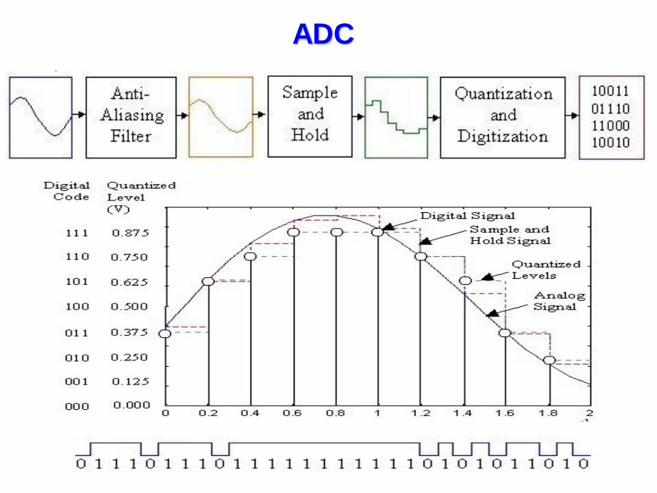
ADC

Sampling
Continuous-time signal discrete-time signal
Analog
world
Digital
world Sampling

Sampling
Taking samples at intervals and don’t know what happens in
between can’t distinguish higher and lower frequencies:
aliasing
How to avoid aliasing?

Nyquist sampling theory
To guarantee that an analog signal can be perfectly
recovered from its sample value
Theory: a signal with maximum of frequency of W Hz must
be sampled at least 2W times per second to make it possible
to reconstruct the original signal from the samples
Nyquist sampling rate: minimum sampling frequency
Nyquist frequency: half the sampling rate
Nyquist range: 0 to Nyquist frequency range
To remove all signal elements above the Nyquist frequency
antialiasing filter

Anti-aliasing filter
0 W 2W =fs 3W 4W
magnitude
frequency
Analog signal spectrum
Anti-aliasing filter response
0 W 2W =fs 3W 4W
magnitude
frequency
Filtered analog signal spectrum

Some examples of sampling frequency
Speech coding/compression ITU G.711, G.729, G.723.1:
fs = 8 kHz T = 1/8000 s = 125μs
Broadband system ITU-T G.722:
fs = 16 kHz T = 1/16 000 s = 62.5μs
Audio CDs:
fs = 44.1 kHz T = 1/44100 s = 22.676μs
Audio hi-fi, e.g., MPEG-2 (moving picture experts group),
AAC (advanced audio coding), MP3 (MPEG layer 3):
fs = 48 kHz T = 1/48 000 s = 20.833μs

Sampling and Hold
Sampling interval Ts (sampling period): time between samples
Sampling frequency fs (sampling rate): # samples per second
Analog signal Sample-and-hold signal
0 1 2 3 4

Quantization
Continuous-amplitude signal discrete-amplitude signal
Quantization step

Coding
Quantized sample N-bit code word
0.0V
0.5V
1.0V
1.5V
0.82V
1.1V 1.25V

Example of quantization and coding
Analog pressures
are recorded,
using a pressure
transducer, as
voltages between
0 and 3V. The
signal must be
quantized using a
3-bit digital code.
Indicate how the
analog voltages
will be converted
to digital values.
Digital code
000
001
010
011
100
101
110
111
Quantization
Level (V)
0.0
0.375
0.75
1.125
1.5
1.875
2.25
2.625
Range of
analog
inputs (V)
0.0-0.1875
0.1875-0.5625
0.5625-0.9375
0.9375-1.3125
1.3125-1.6875
1.6875-2.0625
2.0625-2.4375
2.4375-3.0

Example of quantization and coding
An analog voltage
between -5V and 5V
must be quantized
using 3 bits. Quantize
each of the following
samples, and record
the quantization error
for each:
-3.4V; 0V; .625V
Digital code
100
101
110
111
000
001
010
011
Quantization
Level (V)
-5.0
-3.75
-2.5
-1.25
0.0
1.25
2.5
3.75
Range of analog
inputs (V)
-5.0 -4.375
-4.375-3.125
-3.125-1.875
-1.875-0.625
-0.6250.625
0.6251.875
1.8753.125
3.1255.0

Quantization parameters
Number of bits: N
Full scale analog range: R
Resolution: the gap between levels Q = R/2N
Quantization error = quantized value – actual value
Dynamic range: number of levels, in decibel
Dynamic range = 20log(R/Q) = 20log(2N) = 6.02N dB
Signal-to-noise ratio SNR = 10log(signal power/noise power)
Or SNR = 10log(signal amplitude/noise amplitude)
Bit rate: the rate at which bits are generated
Bit rate = N.fs

Noise removal by quantization
Q/2
Noise
Error
Q
Quantized signal + noise After re-quantization

Non-uniform quantization
Quantization with variable quantization step Q value is
variable
Q value is directly
proportional to signal
amplitude SNR is
constant
Most used in speech Input
Non-
uniform
Uniform
Output

A-law compression curve
1)t(sA
1,
Aln1
))t(sAln(1
A
1)t(s0,
Aln1
)t(sA
)t(s
1
1
1
1
2
- 1.0
- 1.0
1.0
1.0 0
A=87.6
A=1
A=5
s1(t)
s2(t)

ITU G.711 standard Input range Step size Part 1 Part 2 No. code
word Decoding output
0-1 ...
30-31
2 000 0000 ...
1111
0 ... 15
1 ... 31
32-33 ...
62-63
2 001 0000 ...
1111
16 ... 31
33 ... 63
64-67 ...
124-127
4 010 0000 ...
1111
32 ... 47
66 ...
126
128-135 ...
248-255
8 011 0000 ...
1111
48 ... 63
132 ...
252
256-271 ...
496-511
16 100 0000 ...
1111
64 ... 79
264 ...
504
512-543 ...
992-1023
32 101 0000 ...
1111
80 ... 95
528 ...
1008
1024-1087 ...
1984-2047
64 110 0000 ...
1111
96 ...
111
1056 ...
2016
2048-2175 ...
3968-4095
128 111 0000 ...
1111
112 ...
127
2112 ...
4032

ITU G.711 A-law curve
1.0 1/2 1/4 1/8 1/16
1/8 8
6
7
5
4
3
2
1 7/8
6/8
5/8
1.0
4/8
3/8
2/8
0
Code-word format: Sign bit 0/1
Part 1 (3bits) 000 111
Part 2 (16bits) 0000 1111

Example of G.711 code word
A quantized-sample’s value is +121
Sign bit: 0
Part 1: 010
Part 2: 1110
Code word: 00101110
Decoding value: +122
A quantized-sample’s value is -121
Code word: 10101110

Lecture #2: Analog-to-Digital and
Digital-to-Analog conversion
Duration: 2 hr
Outline:
1. A/D conversion
2. D/A conversion

DAC

Anti-imaging filter
0 W 2W =fs 4W = 2fs
frequency
Images Anti-imaging filter
Original two-sided analog signal spectrum
magnitude

Lecture #2
The concept of frequency in
CT & DT signals
Duration: 2 hrs
Outline:
1. CT sinusoidal signals
2. DT sinusoidal signals
3. Relations among frequency variables

Functions:
Plot:
t),tf2cos(A
t),tcos(A)t(xa
t
xa(t)
Acosθ Tp = 1/f
Mathematical description of CT
sinusoidal signals

Properties of CT sinusoidal signals
1. For every fixed value of the frequency f, xa(t) is
periodic: xa(t+Tp) = xa(t)
Tp = 1/f: fundamental period
2. CT sinusoidal signals with different frequencies are
themselves different
3. Increasing the frequency f results in an increase in the
rate of oscillation of the signal (more periods in a
given time interval)

Properties of CT sinusoidal
signals (cont)
For f = 0 Tp = ∞
For f = ∞ Tp = 0
Physical frequency: positive
Mathematical frequency: positive and negative
The frequency range for CT signal:
-∞ < f < +∞
)()(
22)cos()( tjtj
a eA
eA
tAtx

Functions:
Plot:
n),nF2cos(A
n),ncos(A)n(x
Mathematical description of DT
sinusoidal signals

x(n N) x(n) n
n)nF2cos(A)])Nn(F2cos[A 00
k2NF2 0
N
kF0
Properties of DT sinusoidal signals
1. A DT sinusoidal signal x(n) is periodic only if its
frequency F is a rational number

2. DT sinusoidal signals whose frequencies are separated by
an integer multiple of are identical
All are identical
2
)ncos()n2ncos(]n)2cos[()n(x 000
00k
kk
,k2
...,2,1,0k),ncos(A)n(x
Properties of DT sinusoidal signals

3. The highest rate of oscillation in a DT sinusoidal signal is
obtained when:
or, equivalently,
)or(
Properties of DT sinusoidal signals
)2
1For(
2
1F

F0 = 1/8 F0 = 1/4
F0 = 1/2 F0 = 3/4
)2cos()( 0nFnxIllustration for
property 3
-π ≤ Ω ≤ π or -1/2 ≤ F ≤ 1/2: fundamental range

CT signal Sampling DT signal
xa(t) xa(nT)
sf
fF
)tf2cos(A
Sf
nf2cosA
)nTf2cos(A
Normalized
frequency
Sampling of CT sinusoidal signals

CT signals DT signals
f
2 F2 f
2/1F2/1
2/ff2/f
T/T/
ss
Relations among frequency variables
sf
fF

Exercise
Consider the analog signal
a) Determine the minimum sampling rate required to avoid aliasing
b) Suppose that the signal is sampled at the rate fs = 200 Hz. What is
the DT signal obtained after sampling?
c) Suppose that the signal is sampled at the rate fs = 75 Hz. What is
the DT signal obtained after sampling?
d) What is the frequency 0 < f < fs/2 of a sinusoidal signal that yields
samples identical to those obtained in part (c)?
][,100cos3)( stttx

Solution
][,100cos3)( stttx

Solution
][,100cos3)( stttx

Prob.1. An analog signal is converted to digital and then
back to analog signal again, without intermediate DSP.
In what ways will the analog signal at the output differ
from the one at the input?
HW

Prob.2. An analog signal is sampled at its Nyquist rate
1/Ts, and quantized using L quantization levels. The
derived signal is then transmitted on some channels.
(a) Show that the time duration, T, of one bit of the
transmitted binary encoded signal must satisfy
(b) When is the equality sign valid?
HW
)L/(logTT2s

Prob.3. A set of
analog samples,
listed in table 1,
is digitized using
the quantization
table 2.
Determine the
digital codes, the
quantized level,
and the
quantization
error for each
sample.
HW
Digital code
000
001
010
011
100
101
110
111
Quantization
Level (V)
0.0
0.625
1.250
1.875
2.500
3.125
3.750
4.375
Range of analog
inputs (V)
0.0 0.3125
0.31250.9375
0.93751.5625
1.56252.1875
2.18752.8125
2.81253.4375
3.43754.0625
4.06255.0
n 0 1 2 3 4 5 6 7 8
Sample(V) 0.5715 4.9575 0.6250 3.6125 4.0500 0.9555 2.8755 1.5625 2.7500

Prob.4. Consider that you desire an A/D conversion system, such
that the quantization distortion does not exceed ±2% of the full
scale range of analog signal.
(a) If the analog signal’s maximum frequency is 4000 Hz, and
sampling takes place at the Nyquist rate, what value of sampling
frequency is required?
(b) How many quantization levels of the analog signal are needed?
(c) How many bits per sample are needed for the number of levels
found in part (b)?
(d) What is the data rate in bits/s?
HW

Prob.5. An analog voice signal with voltage between
-5V and 5V must be quantized using ITU G.711
standard. Encode each of the following samples; and
record the quantization error for each:
(a) -3.45198 V
(b) 1.01119 V
HW

Prob.6. A 3-bit D/A converter produces a 0 V output
for the code 000 and a 5 V output for the code 111,
with other codes distributed evenly between 0 and 5 V.
Draw the zero order hold output from the converter for
the input below:
111 101 011 101 000 001 011 010 100 110
HW

Prob.7. Consider the analog signal
a) Determine the minimum sampling rate required to avoid aliasing
b) Suppose that the signal is sampled at the rate fs = 5000
samples/sec. What is the DT signal obtained after sampling?
c) What is the analog signal we can reconstruct from the samples if
we use ideal interpolation?
ax (t) 3cos2000 t+5sin6000 t+10cos12000 t
HW

Prob.8. Consider the analog signal
a) Sketch the signal for t from 0 to 30 ms
b) The signal is sampled at the rate fs = 300 samples/s. Determine
the frequency of the DT signal x(n) and show that it is periodic.
c) Compute the sample values in one period of x(n). Sketch x(n) on
the same diagram with x(t). What is the periodic of x(n) in ms?
d) Can you find a sampling rate so that x(n) reaches its peak value?
HW
][,100sin3)( stttx