chapter 2 chemical and radiative effects of hfcs, pfcs, and their
TRANSCRIPT

2Chemical and Radiative Effects of Halocarbons and Their Replacement Compounds
Coordinating Lead AuthorsGuus J.M. Velders (The Netherlands), Sasha Madronich (USA)
Lead AuthorsCathy Clerbaux (France), Richard Derwent (UK), Michel Grutter (Mexico), Didier Hauglustaine (France), Selahattin Incecik (Turkey), Malcolm Ko (USA), Jean-Marie Libre (France), Ole John Nielsen (Denmark), Frode Stordal (Norway), Tong Zhu (China)
Contributing AuthorsDonald Blake (USA), Derek Cunnold (USA), John Daniel (USA), Piers Forster (UK), Paul Fraser (Australia), Paul Krummel (Australia), Alistair Manning (UK), Steve Montzka (USA), Gunnar Myhre (Norway), Simon O’Doherty (UK), David Oram (UK), Michael Prather (USA), Ronald Prinn (USA), Stefan Reimann (Switzerland), Peter Simmonds (UK), Tim Wallington (USA), Ray Weiss (USA)
Review EditorsIvar S.A. Isaksen (Norway), Bubu P. Jallow (Gambia)
IPCC Boek (dik).indb 133 15-08-2005 10:53:32
134 IPCC/TEAP Special Report: Safeguarding the Ozone Layer and the Global Climate System
EXECUTIVE SUMMARY 135
2.1 Introduction 137
2.2 Atmospheric lifetimes and removal processes 1372.2.1 Calculation of atmospheric lifetimes of
halocarbons and replacement compounds 1372.2.2 Oxidation by OH in the troposphere 1402.2.3 Removal processes in the stratosphere 1422.2.4 Other sinks 1422.2.5 Halogenated trace gas steady-state
lifetimes 143
2.3 Concentrations of CFCs, HCFCs, HFCs and PFCs 1432.3.1 Measurements of surface concentrations and growth rates 1432.3.2 Deriving global emissions from observed
concentrations and trends 1472.3.3 Deriving regional emissions from observed
concentrations 149
2.4 Decomposition and degradation products from HCFCs, HFCs, HFEs, PFCs and NH3 1512.4.1 Degradation products from HCFCs, HFCs and HFEs 1512.4.2 Trifluoroacetic acid (TFA, CF
3C(O)OH)) 154
2.4.3 Other halogenated acids in the environment 155
2.4.4 Ammonia (NH3) 155
2.5 Radiative properties and global warming potentials 1562.5.1 Calculation of GWPs 1562.5.2 Calculation of radiative forcing 1572.5.3 Other aspects affecting GWP
calculations 1582.5.4 Reported values 1592.5.5 Future radiative forcing 163
2.6 Impacts on air quality 1662.6.1 Scope of impacts 1662.6.2 Global-scale air quality impacts 1672.6.3 Urban and regional air quality 169
References 173
Contents
IPCC Boek (dik).indb 134 15-08-2005 10:53:33

Chapter 2: Chemical and Radiative Effects of Halocarbons and Their Replacement Compounds 135
EXECUTIVE SUMMARY
• Human-made halocarbons, including chlorofluorocarbons (CFCs), perfluorocarbons (PFCs), hydrofluorocarbons (HFCs) and hydrochlorofluorocarbons (HCFCs), are effective absorbers of infrared radiation, so that even small amounts of these gases contribute to the radiative forcing of the climate system. Some of these gases and their replacements also contribute to stratospheric ozone depletion and to the deterioration of local air quality.
Concentrations and radiative forcing of fluorinated gases and replacement chemicals• HCFCs of industrial importance have lifetimes in the range
1.3–20 years. Their global-mean tropospheric concentrations in 2003, expressed as molar mixing ratios (parts per trillion, ppt, 10–12), were 157 ppt for HCFC-22, 16 ppt for HCFC-141b, and 14 ppt for HCFC-142b.
• HFCs of industrial importance have lifetimes in the range 1.4–270 years. In 2003 their observed atmospheric concentrations were 17.5 ppt for HFC-23, 2.7 ppt for HFC-125, 26 ppt for HFC-134a, and 2.6 ppt for HFC-152a.
• The observed atmospheric concentrations of these HCFCs and HFCs can be explained by anthropogenic emissions, within the range of uncertainties in calibration and emission estimates.
• PFCs and SF6 have lifetimes in the range 1000–50,000 years
and make an essentially permanent contribution to radiative forcing. Concentrations in 2003 were 76 ppt for CF
4, 2.9
ppt for C2F
6, and 5 ppt for SF
6. Both anthropogenic and
natural sources of CF4 are needed to explain its observed
atmospheric abundance.• Global and regional emissions of CFCs, HCFCs and HFCs
have been derived from observed concentrations and can be used to check emission inventory estimates. Global emissions of HCFC-22 have risen steadily over the period 1975–2000, whereas those of HCFC-141b, HCFC-142b and HFC-134a started to increase quickly in the early 1990s. In Europe, sharp increases in emissions occurred for HFC-134a over 1995–1998 and for HFC-152a over 1996–2000, with some levelling off of both through 2003.
• Volatile organic compounds (VOCs) and ammonia (NH3),
which are considered as replacement species for refrigerants or foam blowing agents, have lifetimes of several months or less, hence their distributions are spatially and temporally variable. It is therefore difficult to quantify their climate impacts with single globally averaged numbers. The direct and indirect radiative forcings associated with their use as substitutes are very likely to have a negligible effect on global climate because of their small contribution to existing VOC and NH
3 abundances in the atmosphere.
• The lifetimes of many halocarbons depend on the concentration of the hydroxyl radical (OH), which might change in the 21st century as a result of changes in emissions of carbon monoxide, natural and anthropogenic VOCs,
and nitrogen oxides, and as a result of climate change and changes in tropospheric ultraviolet radiation. The sign and magnitude of the future change in OH concentrations are uncertain, and range from –18 to +5% for the year 2100, depending on the emission scenario. For the same emissions of halocarbons, a decrease in future OH would lead to higher concentrations of these halocarbons and hence would increase their radiative forcing, whereas an increase in future OH would lead to lower concentrations and smaller radiative forcing.
• The ODSs have contributed 0.32 W m–2 (13%) to the direct radiative forcing of all well-mixed greenhouse gases, relative to pre-industrial times. This contribution is dominated by CFCs. The current (2003) contributions of HFCs and PFCs to the total radiative forcing by long-lived greenhouse gases are 0.0083 W m–2 (0.31%) and 0.0038 W m–2 (0.15%), respectively.
• Based on the emissions reported in Chapter 11 of this report, the estimated radiative forcing of HFCs in 2015 is in the range of 0.019–0.030 W m–2 compared with the range 0.022–0.025 W m–2 based on projections in the IPCC Special Report on Emission Scenarios (SRES). Based on SRES projections, the radiative forcing of HFCs and PFCs corresponds to about 6–10% and 2%, respectively, of the total estimated radiative forcing due to CFCs and HCFCs in 2015.
• Projections of emissions over longer time scales become more uncertain because of the growing influence of uncertainties in technological practices and policies. However, based on the range of SRES emission scenarios, the contribution of HFCs to radiative forcing in 2100 could range from 0.1 to 0.25 W m–2 and of from PFCs 0.02 to 0.04 W m–2. In comparison, the forcing from carbon dioxide (CO
2) in these
scenarios ranges from about 4.0 to 6.7 W m–2 in 2100.• Actions taken under the Montreal Protocol and its
Adjustments and Amendments have led to the replacement of CFCs with HCFCs, HFCs, and other substances, and to changing of industrial processes. These actions have begun to reduce atmospheric chlorine loading. Because replacement species generally have lower global warming potentials (GWPs), and because total halocarbon emissions have decreased, the total CO
2-equivalent emission (direct
GWP-weighted using a 100-year time horizon) of all halocarbons has also been reduced. The combined CO
2-
equivalent emissions of CFCs, HCFCs and HFCs decreased from a peak of about 7.5 ± 0.4 GtCO
2-eq yr–1 around 1990
to about 2.5 ± 0.2 GtCO2-eq yr–1 in the year 2000, which
corresponds to about 10% of that year’s CO2 emissions from
global fossil-fuel burning.
Banks• Continuing observations of CFCs and other ODSs in the
atmosphere enable improved validation of estimates of the lag between production and emission to the atmosphere, and of the associated banks of these gases. Because new
IPCC Boek (dik).indb 135 15-08-2005 10:53:33

136 IPCC/TEAP Special Report: Safeguarding the Ozone Layer and the Global Climate System
production of ODSs has been greatly reduced, annual changes in their concentrations are increasingly dominated by releases from existing banks. The decrease in the atmospheric concentrations of several gases is placing tighter constraints on their derived emissions and banks. This information provides new insights into the significance of banks and end-of-life options for applications using HCFCs and HFCs as well.
• Current banked halocarbons will make a substantial contribution to future radiative forcing of climate for many decades unless a large proportion of these banks is destroyed. Large portions of the global inventories of CFCs, HCFCs and HFCs currently reside in banks. For example, it is estimated that about 50% of the total global inventory of HFC-134a currently resides in the atmosphere and 50% resides in banks. One top-down estimate based on past reported production and on detailed comparison with atmospheric-concentration changes suggests that if the current banks of CFCs, HCFCs and HFCs were to be released to the atmosphere, their corresponding GWP-weighted emissions (using a 100-year time horizon) would represent about 2.6, 3.4 and 1.2 GtCO
2-eq, respectively.
• If all the ODSs in banks in 2004 were not released to the atmosphere, the direct positive radiative forcing could be reduced by about 0.018–0.025 W m–2 by 2015. Over the next two decades this positive radiative forcing change is expected to be about 4–5% of that due to carbon dioxide emissions over the same period.
Global warming potentials (GWPs)• The climate impact of a given mass of a halocarbon emitted
to the atmosphere depends on its radiative properties and atmospheric lifetime. The two can be combined to compute the global warming potential (GWP), which is a proxy for the climate effect of a gas relative to the emission of a pulse of an equal mass of CO
2. Multiplying emissions of a gas by
its GWP gives the CO2-equivalent emission of that gas over
a given time horizon.• The GWP value of a gas is subject to change as better
estimates of the radiative forcing and the lifetime associated with the gas or with the reference gas (CO
2) become
available. The GWP values (over 100 years) recommended in this report (Table 2.6) have been modified, depending on the gas, by –16% to +51%, compared with values reported in IPCC (1996), which were adopted by the United Nations Framework Convention on Climate Change (UNFCCC) for use in national emission inventories. Some of these changes have already been reported in IPCC (2001).
• HFC-23 is a byproduct of the manufacturing of HCFC-22 and has a substantial radiative efficiency. Because of its long lifetime (270 years) its GWP is the largest of the HFCs, at 14,310 for a 100-year time horizon.
Degradation products• The intermediate degradation products of most long-
lived CFCs, HCFCs and HFCs have shorter lifetimes than the source gases, and therefore have lower atmospheric concentrations and smaller radiative forcing. Intermediate products and final products are removed from the atmosphere via deposition and washout processes and may accumulate in oceans, lakes and other reservoirs.
• Trifluoroacetic acid (TFA) is a persistent degradation product of some HFCs and HCFCs, with yields that are known from laboratory studies. TFA is removed from the atmosphere mainly by wet deposition. TFA is toxic to some aquatic life forms at concentrations at concentrations approaching 1 mg L–1. Current observations show that the typical concentration of TFA in the oceans is 0.2 µg L–1, but concentrations as high as 40 µg L–1 have been observed in the Dead Sea and Nevada lakes.
• New studies based on measured concentrations of TFA in sea water provide stronger evidence that the cumulative source of TFA from the degradation of HFCs is smaller than natural sources, which, however, have not been fully identified. The available environmental risk assessment and monitoring data indicate that the source of TFA from the degradation of HFCs is not expected to result in environmental concentrations capable of significant ecosystem damage.
Air-quality effects• HFCs, PFCs, other replacement gases such as organic
compounds, and their degradation intermediates are not expected to have a significant effect on global concentrations of OH radicals (which essentially determine the tropospheric self-cleaning capacity), because global OH concentrations are much more strongly influenced by carbon monoxide, methane and natural hydrocarbons.
• The local impact of hydrocarbon and ammonia substitutes for air-conditioning, refrigeration and foam-blowing applications can be estimated by comparing their anticipated emissions to local pollutant emissions from all sources. Small but not negligible impacts could occur near highly localized emission sources. However, even small impacts may be of some concern in urban areas that currently fail to meet air quality standards.
IPCC Boek (dik).indb 136 15-08-2005 10:53:34

Chapter 2: Chemical and Radiative Effects of Halocarbons and Their Replacement Compounds 137
2.1 Introduction
The depletion of ozone in the stratosphere and the radiative forcing of climate change are caused by different processes. Chlorine and bromine released from chlorofluorocarbons (CFCs), halons and other halogen-containing species emitted in the last few decades are primarily responsible for the depletion of the ozone layer in the stratosphere. Anthropogenic emissions of carbon dioxide, methane, nitrous oxide and other green-house gases are, together with aerosols, the main contributors to the change in radiative forcing of the climate system over the past 150 years. The possible adverse effects of both global environmental issues are being dealt with in different political arenas. The Vienna Convention and the Montreal Protocol are designed to protect the ozone layer, whereas the United Nations Framework Convention on Climate Change (UNFCCC) and the Kyoto Protocol play the same role for the climate system. However these two environmental issues interact both with respect to the trade-off in emissions of species as technology evolves, and with respect to the chemical and physical proc-esses in the atmosphere. The chemical and physical processes of these interactions and their effects on ozone are discussed in Chapter 1. This chapter focuses on the atmospheric abun-dance and radiative properties of CFCs, hydrochlorofluorocar-bons (HCFCs), hydrofluorocarbons (HFCs), perfluorocarbons (PFCs), and their possible replacements, as well as on their deg-radation products, and on their effects on global, regional and local air quality. The total amount, or burden, of a gas in the atmosphere is determined by the competing processes of its emission into and its removal from the atmosphere. Whereas emissions of most of the gases considered here are primarily a result of human activities, their rates of removal are largely determined by com-plex natural processes that vary both spatially and temporally, and may differ from gas to gas. Rapid removal implies a short atmospheric lifetime, whereas slow removal and therefore a longer lifetime means that a given emission rate will result in a larger atmospheric burden. The concept of the atmospheric life-time of a gas, which summarizes its destruction patterns in the atmosphere, is therefore central to understanding its atmospher-ic accumulation. Section 2.2 discusses atmospheric lifetimes, how they are calculated, their influence on the global distribu-tion of halocarbons, and their use in evaluating the effects of various species on the ozone layer and climate change under different future scenarios. Section 2.3 discusses the observed atmospheric abundance of CFCs, HCFCs, HFCs and PFCs, as well as emissions derived from these observations. Section 2.4 discusses the decomposition products (e.g., trifluoroacetic acid, TFA) of these species and their possible effects on ecosystems. Halocarbons, as well as carbon dioxide and water vapour, are greenhouse gases; that is, they allow incoming solar shortwave radiation to reach the Earth’s surface, while absorbing outgoing longwave radiation. The radiative forcing of a gas quantifies its ability to perturb the Earth’s radiative energy budget, and can be either positive (warming) or negative (cooling). The global
warming potential (GWP) is an index used to compare the cli-mate impact of a pulse emission of a greenhouse gas, over time, relative to the same mass emission of carbon dioxide. Radiative forcings and GWPs are discussed in Section 2.5. The concen-trations of emitted species and their degradation products de-termine to a large extent their atmospheric impacts. Some of these concentrations are currently low but might increase in the future to levels that could cause environmental impacts. Some of the species being considered as replacements for ozone-depleting substances (ODSs), in particular hydrocarbons (HCs) and ammonia (NH
3), are known to cause deterioration of
tropospheric air quality in urban and industrialized continen-tal areas, are involved in regulation of acidity and precipitation (ammonia), and could perturb the general self-cleaning (oxidiz-ing) capacity of the global troposphere. These issues are con-sidered in Section 2.6, where potential increments in reactivity from the replacement compounds are compared with the reac-tivity of current emissions from other sources.
2.2 Atmospheric lifetimes and removal processes
2.2.1 Calculation of atmospheric lifetimes of halocarbons and replacement compounds
To evaluate the environmental impact of a given gas molecule, one needs to know, first, how long it remains in the atmosphere. CFCs, HCFCs, HFCs, PFCs, hydrofluoroethers (HFEs), HCs and other replacement species for ODSs are chemically trans-formed or physically removed from the atmosphere after their release. Known sinks for halocarbons and replacement gases include photolysis; reaction with the hydroxyl radical (OH), the electronically excited atomic oxygen (O(1D)) and atomic chlorine (Cl); uptake in oceanic surface waters through dissolu-tion; chemical and biological degradation processes; biological degradation in soils; and possibly surface reactions on minerals. For other trace gases, such as NH
3, uptake by aerosols, cloud
removal, aqueous-phase chemistry, and surface deposition also provide important sink processes. A schematic of the various removal processes affecting the atmospheric concentration of the considered species is provided in Figure 2.1. Individual removal processes have various impacts on differ-ent gases in different regions of the atmosphere. The dominant process (the one with the fastest removal rate) controls the local loss of a gas. For example, reaction with OH is the dominant re-moval process for many hydrogenated halocarbons in both the troposphere and stratosphere. For those same gases, reactions with O(1D) and Cl play a large role only in the stratosphere. The determination of the spatial distribution of the sink strength of a trace gas is of interest because it is relevant to both the calcula-tion of the atmospheric lifetime and the environmental impact of the substance. The lifetimes of atmospheric trace gases have been recently re-assessed by the IPCC (2001, Chapter 4) and by the WMO Scientific Assessment of Ozone Depletion (WMO, 2003, Chapter 1). Below is an updated summary of key features and methods used to determine the lifetimes.
IPCC Boek (dik).indb 137 15-08-2005 10:53:34

138 IPCC/TEAP Special Report: Safeguarding the Ozone Layer and the Global Climate System
For a given trace gas, each relevant sink process, such as pho-todissociation or oxidation by OH, contributes to the additive first-order total loss frequency, l, which is variable in space and time. A local lifetime τ
local can be defined as the inverse of l
evaluated at a point in space (x, y, z) and time (t):
τlocal
= 1/l(x, y, z, t) (2.1)
The global instantaneous atmospheric lifetime of the gas is ob-tained by integrating l over the considered atmospheric domain. The integral must be weighted by the distribution of the trace gas on which the sink processes act. If C(x, y, z, t) is the distri-bution of the trace gas , then the global instantaneous lifetime derived from the budget can be defined as:
τglobal
= ∫ C dv / ∫ C l dv (2.2)
where dv is an atmospheric volume element. This expression
can be averaged over a year to determine the global and annu-ally averaged lifetime. The sinks that dominate the atmospheric lifetime are those that have significant strength on a mass or molecule basis, that is, where loss frequency and atmospheric abundance are correlated. Because the total loss frequency l is the sum of the individual sink-process frequencies, τ
global can
also be expressed in terms of process lifetimes:
1/τglobal
= 1/τtropospheric OH
+ 1/τphotolysis
+ 1/τocean
+ 1/τ
scavenging + 1/τ
other processes (2.3)
It is convenient to consider lifetime with respect to individual sink processes limited to specific regions, for example, reaction with OH in the troposphere. However, the associated burden must always be global and include all communicating reservoirs in order for Equation (2.3) to remain valid. In Equation (2.2) the numerator is therefore integrated over the whole atmospheric domain and the denominator is integrated over the domain in
PFCs
SF6
CFCs
Halons
CFCs
Halons
PFCs
SF6
HCFCs
HFCs
HFEsCH
3CCl
3
Land Ocean Land
DegradationProducts
DegradationProducts
DegradationProducts
DegradationProducts
O1D
OH
UV
F
BrCl
O3
O1D
H2O
light, H2O
lightTFA
OH
HO2
Removal
HCs CO2
HClNO NO
2
OH
NH3
Aerosols
Mesosphere
Stratosphere
Troposphere
Figure 2.1. Schematic of the degradation pathways of CFCs, HCFCs, HFCs, PFCs, HFEs, HCs and other replacements species in the various atmospheric reservoirs. Colour coding: brown denotes halogens and replacement species emitted and orange their degradation products in the atmosphere; red denote radicals; green arrows denote interaction with soils and the biosphere; blue arrows denote interaction with the hydrological cycle; and black the aerosol phase.
IPCC Boek (dik).indb 138 15-08-2005 10:53:35

Chapter 2: Chemical and Radiative Effects of Halocarbons and Their Replacement Compounds 139
which the individual sink process is considered. In the case of τ
tropospheric OH, the convention is that integration is performed over
the tropospheric domain. The use of different domains or dif-ferent definitions for the troposphere can lead to differences of
10% in the calculated value (Lawrence et al., 2001). A more detailed discussion of lifetimes is given in Box 2.1; the reader is referred to the cited literature for further informa-tion.
Box 2.1. Global atmospheric, steady-state and perturbation lifetimes
The conservation equation of a given trace gas in the atmosphere is given by:
dB(t)/dt = E(t) – L(B, t) (1)
where the time evolution of the burden, B(t) [kg] = ∫ C dv, is given by the emissions, E(t) [kg s–1], minus the loss, L(B, t) [kg s–1] = ∫ C l dv. The emission is an external parameter. The loss of the gas may depend on its concentration as well as that of other gases. The global instantaneous atmospheric lifetime (also called ‘burden lifetime’ or ‘turnover lifetime’), defined in Equation (2.2), is given by the ratio τ
global = B(t)/L(t). If this quantity is constant in time, then the conservation equation takes
on a much simpler form:
dB(t)/dt = E(t) – B(t)/τglobal
(2)
Equation (2) is for instance valid for a gas whose local chemical lifetime is constant in space and time, such as the noble gas radon (Rn), whose lifetime is fixed by the rate of its radioactive disintegration. In such a case the mean atmospheric lifetime equals the local lifetime: the lifetime that relates source strength to global burden is exactly the decay time of a perturbation. The global atmospheric lifetime characterizes the time to achieve an e-fold (63.2%, see ‘lifetime’ in glossary) decrease of the global atmospheric burden. Unfortunately, τ
global is truly a constant only in very limited circumstances because both C and l
change with time. Note that when in steady-state (i.e., with unchanging burden), Equation (1) implies that the source strength is equal to the sink strength. In this case, the steady-state lifetime (τSS
global) is a scale factor relating constant emissions to the
steady-state burden of a gas (BSS = τSSglobal
E).
In the case that the loss rate depends on the burden, Equation (2) must be modified. In general, a more rigorous (but still approximate) solution can be achieved by linearizing the problem. The perturbation or pulse decay lifetime (τ
pert) is defined
simply as:
1/τpert
= ∂L(B, t)/∂B (3)
and the correct form of the conservation equation is (Prather, 2002):
dΔB(t)/dt = ΔΕ(t) – ΔB(t)/τpert
(4)
where ΔB(t) is the perturbation to the steady-state background B(t) and ΔΕ(t) is an emission perturbation (pulse or constant increment). Equation (4) is particularly useful for determining how a one-time pulse emission may decay with time, which is a quantity needed for GWP calculation. For some gases, the perturbation lifetime is considerably different from the steady-state lifetime (i.e., the lifetime that relates source strength to steady-state global burden is not exactly equal to the decay time of a perturbation). For example, if the abundance of CH
4 is increased above its present-day value by a one-time emission, the
time it would take for CH4 to decay back to its background value is longer than its global unperturbed atmospheric lifetime.
This occurs because the added CH4 causes a suppression of OH, which in turn increases the background abundance of CH
4.
Such feedbacks cause the time scale of a perturbation (τpert
) to differ from the steady-state lifetime (τSSglobal
). In the limit of small perturbations, the relation between the perturbation lifetime of a gas and its global atmospheric lifetime can be derived from the simple budget relationship τ
pert = τSS
global/(1 – f), where f = dln(τ
globalSS)/dln(B) is the sensitivity coefficient (without a
feedback on lifetime, f = 0 and τpert
is identical to τSSglobal
). The feedback of CH4 on tropospheric OH and its own lifetime has
been re-evaluated with contemporary global chemical-transport models (CTMs) as part of an IPCC intercomparison exercise (IPCC, 2001, Chapter 4). The calculated OH feedback, dln(OH)/dln(CH
4), was consistent among the models, indicating that
tropospheric OH abundances decline by 0.32% for every 1% increase in CH4. When other loss processes for CH
4 (loss to
stratosphere, soil uptake) were included, the feedback factor reduced to 0.28 and the ratio τpert
/τSSglobal
was 1.4. For a single pulse, this 40% increase in the integrated effect of a CH
4 perturbation does not translate to a 40% larger burden in the per-
IPCC Boek (dik).indb 139 15-08-2005 10:53:36

140 IPCC/TEAP Special Report: Safeguarding the Ozone Layer and the Global Climate System
Figure 2.2 shows the time evolution of the remaining fraction of several constituents in the atmosphere after their pulse emission at time t = 0. This figure illustrates the impact of the lifetime of the constituent on the decay of the perturbation. The half-life is the time required to remove 50% of the initial mass injected and the e-fold time is the time required to remove 63.2%. As mentioned earlier, a pulse emission of most gases into the at-mosphere decays on a range of time scales until atmospheric transport and chemistry redistribute the gas into its longest-lived decay pattern. Most of this adjustment occurs within 1 to 2 years as the gas mixes throughout the atmosphere. The final e-fold decay occurs on a time scale very close, but not exactly equal, to the steady-state lifetime used to prepare Figure 2.2 and Table 2.6. Note that the removal of CO
2 from the atmosphere
cannot be adequately described by a single, simple exponential lifetime (see IPCC, 1994, and IPCC, 2001, for a discussion). The general applicability of atmospheric lifetimes breaks down for gases and pollutants whose chemical losses or local lifetimes vary in space and time and the average duration of the lifetimes is weeks rather than years or months. For these gases the value of the global atmospheric lifetime is not unique and depends on the location (and season) and the magnitude of the emission (see Box 2.1). The majority of halogen-contain-ing species and ODS-replacement species considered here have atmospheric lifetimes greater than two years, much longer than tropospheric mixing times; hence their lifetimes are not signifi-
cantly altered by the location of sources within the troposphere. When lifetimes are reported for gases in Table 2.6, it is assumed that the gases are uniformly mixed throughout the troposphere. This assumption is less accurate for gases with lifetimes shorter than one year. For such short-lived gases (e.g., HCs, NH
3), re-
ported values for a single global lifetime, ozone depletion po-tential (ODP) or GWP become inappropriate.
2.2.2 Oxidation by OH in the troposphere
The hydroxyl radical (OH) is the primary cleansing agent of the lower atmosphere, and in particular it provides the dominant sink for HCFCs, HFCs, HCs and many chlorinated hydrocar-bons. The steady-state lifetimes of these trace gases are deter-mined by the morphology of the species’ distribution, the kinet-ics of the reaction with OH, and the OH distribution. The local abundance of OH is mainly controlled by the local abundances of nitrogen oxides (NO
x = NO + NO
2), CO, CH
4 and higher hy-
drocarbons, O3, and water vapour, as well as by the intensity of
solar ultraviolet radiation. The primary source of tropospheric OH is a pair of reactions that start with the photodissociation of O
3 by solar ultraviolet radiation:
O3 + hν → O(1D) + O
2 [2.1]
O(1D) + H2O → OH + OH [2.2]
turbation but rather to a lengthening of the duration of the perturbation. If the increased emissions are maintained to steady-state, then the 40% increase does translate to a larger burden (Isaksen and Hov, 1987).
The pulse lifetime is the lifetime that should be used in the GWP calculation (in particular in the case of CH4). For the long-
lived halocarbons, l is approximately constant in time and C can be approximated by the steady-state distribution in order to calculate the steady-state lifetimes reported in Table 2.6. In this case, Equation (2) is approximately valid and the decay lifetime of a pulse is taken to be the same as the steady-state global atmospheric lifetime.
In the case of a constant increment in emissions, at steady-state, Equation (4) shows that steady-state lifetime of the pertur-bation (τSS
pert) is a scaling factor relating the steady-state perturbation burden (ΔBSS) to the change in emission (ΔBSS = τSS
pert
ΔE). Furthermore, Prather (1996, 2002) has also shown that the integrated atmospheric abundance following a single pulse emission is equal to the product of the amount emitted and the perturbation steady-state lifetime for that emission pattern. The steady-state lifetime of the perturbation is then a scaling factor relating the emission pulse to the time-integrated burden of that pulse.
Lifetimes can be determined using global tropospheric models by simulating the injection of a pulse of a given gas and watching the decay of this added amount. This decay can be represented by a sum of exponential functions, each with its own decay time. These exponential functions are the chemical modes of the linearized chemistry-transport equations of a global model (Prather, 1996). In the case of a CH
4 addition, the longest-lived mode has an e-fold time of 12 years, which is very
close to the steady-state perturbation lifetime of CH4 and carries most of the added burden. In the case of a carbon monoxide
(CO), HCFCs or HCs addition, this mode is also excited, but at a much-reduced amplitude, which depends on the amount of gas added (Prather, 1996; Daniel and Solomon, 1998). The pulse of added CO, HCFCs or HCs causes a build-up of CH
4
while the added burden of the gas persists, by causing the concentration of OH to decrease and thus the lifetime of CH4 to
increase temporarily. After the initial period defined by the photochemical lifetime of the injected trace gas, this built-up CH4
decays in the same manner as would a direct pulse of CH4. Thus, changes in the emissions of short-lived gases can generate
long-lived perturbations, a result which is also shown in global models (Wild et al., 2001; Derwent et al., 2001).
IPCC Boek (dik).indb 140 15-08-2005 10:53:36

Chapter 2: Chemical and Radiative Effects of Halocarbons and Their Replacement Compounds 141
In polluted regions and in the upper troposphere, photodissocia-tion of other trace gases, such as peroxides, acetone and formal-dehyde (Singh et al., 1995; Arnold et al., 1997), may provide the dominant source of OH (e.g., Folkins et al., 1997; Prather and Jacob, 1997; Müller and Brasseur, 1999; Wennberg et al., 1998). OH reacts with many atmospheric trace gases, in most cases as the first and rate-determining step of a reaction chain that leads to more or less complete oxidation of the compound. These chains often lead to formation of an HO
2 radical, which
then reacts with O3 or NO to recycle back to OH. Tropospheric
OH and HO2 are lost through radical-radical reactions that lead
to the formation of peroxides, or by reaction with NO2 to form
HNO3. The sources and sinks of OH involve most of the fast
photochemistry of the troposphere. The global distribution of OH radicals cannot be observed directly because of the difficulty in measuring its small concen-trations (of about 106 OH molecules per cm3 on average dur-ing daylight in the lower free troposphere) and because of high variability of OH with geographical location, time of day and season. However, indirect estimates of the average OH concen-tration can be obtained from observations of atmospheric con-centrations of trace gases, such methyl chloroform (CH
3CCl
3),
that are removed mostly by reaction with OH (with rate con-stants known from laboratory studies) and whose emission his-tory is relatively well known. The lifetime of CH
3CCl
3 is often
used as a reference number to derive the lifetime of other spe-cies (see Section 2.2.5) and, by convention, provides a measure of the global OH burden. Observations over a long time (years to decades) can provide estimates of long-term OH trends that would change the lifetimes, ODPs and GWPs of some halo-carbons, and increase or decrease their impacts relative to the
current values. There is an ongoing debate in the literature about the emis-sions and lifetime of CH
3CCl
3 and hence on the deduced vari-
ability of OH concentrations over the last 20 years. Prinn et al. (2001) analyzed a 22-year record of global CH
3CCl
3 measure-
ments and emission estimates and suggested that the trend in global OH over that period was –0.66 ± 0.57% yr–1. Prinn and Huang (2001) analyzed the record only from 1978 to 1993 and deduced a trend of +0.3% yr–1 using the same emissions as Krol et al. (1998). These results through 1993 are essentially consist-ent with the conclusions of Krol et al. (1998, 2001), who used the same measurements and emission record but an independ-ent calculation technique to infer a trend of +0.46 ± 0.6% yr–1 between 1978 and 1994. However, Prinn et al. (2001) inferred a larger interannual and inter-decadal variability in global OH than Krol et al. (1998, 2001). Prinn et al. (2001) also inferred that OH concentrations in the late 1990s were lower than those in the late 1970s to early 1980s, in agreement with the longer CH
3CCl
3 lifetime reported by Montzka et al. (2000) for
1998–1999 relative to the Prinn et al. (2001) value for the full-period average. A recent study by Krol and Lelieveld (2003) indicated a larger variation of OH of +12% during 1978–1990, followed by a decrease slightly larger than 12% in the decade 1991–2000. Over the entire 1978–2000 period, the study found that the overall change was close to zero. As discussed by Prinn et al. (1995, 2001), Krol and Lelieveld (2003) and Krol et al. (2003), inferences regarding CH
3CCl
3
lifetimes or trends in OH are sensitive to errors in the absolute magnitude of estimated emissions and to the estimates of other sinks (stratospheric loss, ocean sink). The errors on emissions could be significant and enhanced during the late 1990s because the annual emissions of CH
3CCl
3 were dropping precipitously
at the time. These difficulties in the use of CH3CCl
3 to infer the
trend in OH have also been pointed out by Jöckel et al. (2003), who suggested the use of other dedicated tracers to estimate the global OH distribution. The fluctuations in global OH derived from CH
3CCl
3 meas-
urements are in conflict with observed CH4 growth rates and
with model calculations. Karlsdottir and Isaksen (2000) and Dentener et al. (2003a,b) present multi-dimensional model re-sults for the period 1980–1996 and 1979–1993, respectively. These studies produce increases in mean global tropospheric OH levels of respectively 0.41% yr–1 and 0.25% yr–1 over the considered periods. These changes are driven largely by in-creases in low-latitude emissions of NO
x and CO, in the case
of Karlsdottir and Isaksen (2000), and also by changes in strat-ospheric ozone and meteorological variability, in the case of Dentener et al. (2003a,b). The modelling study by Warwick et al. (2002) also stressed the importance of meteorological inter-annual variability on global OH and on the growth rate of CH
4
in the atmosphere. Wang et al. (2004) also derived a positive trend in OH of +0.63% yr–1 over the period 1988–1997. Their calculated trend in OH is primarily associated with the negative trend in overhead column ozone. We note however that their forward simulations did not account for the interannual vari-
�������������������������������������
���
����
����
����
���
���
���
���
���
���
���
�������������������������������� �� ��� ����
���������
������
��������
���
��������
������
���
���
���
Figure 2.2. Decay of a pulse emission, released into the atmosphere at time t = 0, of various gases with atmospheric lifetimes spanning 1.4 years (HFC-152a) to 50,000 years (CF
4). The CO
2 curve is based on an
analytical fit to the CO2 response function (WMO, 1999, Chapter 10).
IPCC Boek (dik).indb 141 15-08-2005 10:53:38

142 IPCC/TEAP Special Report: Safeguarding the Ozone Layer and the Global Climate System
ability of all the variables that affect OH and were conditional on their assumed emissions being correct. Because of its dependence on CH
4 and other pollutants, the
concentration of tropospheric OH is likely to have changed since the pre-industrial era and is expected to change in the future. Pre-industrial OH is likely to have been different than it is today, but because of the counteracting effects of higher concentrations of CO and CH
4 (which decrease OH) and higher
concentrations of NOx and O
3 (which increase OH) there is lit-
tle consensus on the magnitude or even the sign of this change. Several model studies have suggested that weighted global mean OH has decreased from pre-industrial time to the present day by less than 10% (Berntsen et al., 1997; Wang and Jacob, 1998; Shindell et al., 2001; Lelieveld et al., 2002). Other studies have reported larger decreases in global OH of 16% (Mickley et al., 1999) and 33% (Hauglustaine and Brasseur, 2001). The model study by Lelieveld et al. (2002) suggests that during the past century OH concentrations decreased substantially in the marine troposphere by reaction with CH
4 and CO; however, on
a global scale, this decrease has been offset by an increase over the continents associated with large emissions of NO
x.
As for future changes in OH, the IPCC (2001, Chapter 4) used scenarios reported in the IPCC Special Report on Emissions Scenarios (SRES, IPCC, 2000) and a comparison of results from 14 models to predict that global OH could de-crease by 10% to 18% by 2100 for five emission scenarios, and increase by 5% for one scenario that assumed large decreases in CH
4 and other ozone precursor emissions. Based on a dif-
ferent emission scenario Wang and Prinn (1999) projected a decrease in OH concentrations of 16 ± 3%. In addition to emis-sion changes, future increases in direct and indirect green-house gases could also induce changes in OH through direct participation in OH-controlling chemistry, indirectly through stratospheric ozone changes that could change solar ultraviolet in the troposphere, and potentially through climate change ef-fects on biogenic emissions, temperature, humidity and clouds. Changes in tropospheric water could have important chemi-cal repercussions, because the reaction between water vapour and electronically excited oxygen atoms constitutes the major source of tropospheric OH (Reaction [2.1]). So in a warmer and potentially wetter climate, the abundance of OH is expected to increase.
2.2.3 Removal processes in the stratosphere
Stratospheric in situ sinks for halocarbons and ODS replace-ments include photolysis and homogeneous gas-phase reactions with OH, Cl and O(1D). Because about 90% of the burden of well-mixed gases resides in the troposphere, stratospheric re-moval does not contribute much to the atmospheric lifetimes of gases that are removed efficiently in the troposphere. For most of the HCFCs and HFCs considered in this report, stratospheric removal typically accounts for less than 10% of the total loss. However, stratospheric removal is important for determining the spatial distributions of a source gas and its degradation products
in the stratosphere. These distributions depend on the competi-tion between local photochemical removal processes and the transport processes that carry the material from the entry point (mainly at the tropical tropopause) to the upper stratosphere and the extra-tropical lower stratosphere. Observations show that the stratospheric mixing ratios of source gases decrease with altitude and can be described at steady-state by a local exponen-tial scale height at each latitude. Theoretical calculations show that the local scale height is proportional to the square root of the local lifetime (Ehhalt et al., 1998). Previous studies (Hansen et al., 1997; Christidis et al., 1997; Jain et al., 2000) showed that depending on the values of the as-sumed scale height in the stratosphere, the calculated radiative forcing for CFC-11 can differ by as much as 30%. Thus, accu-rate determination of the GWP of a gas also requires knowing its scale height in the stratosphere. Again, observations will be useful for verifying model-calculated scale heights. Other diag-nostics, such as the age of air (see glossary), will improve our confidence in the models’ ability to simulate the transport in the atmosphere and accurately predict the scale heights appropriate for radiative forcing calculations. Perfluorinated compounds, such as PFCs, SF
6 and SF
5CF
3,
have limited use as ODS replacements is limited (see Chapter 10). The carbon-fluorine bond is remarkably strong and resist-ant to chemical attack. Atmospheric removal processes for PFCs are extremely slow and these compounds have lifetimes measured in thousands of years. Photolysis at short wave-lengths (e.g., Lyman-α at 121.6 nm in the mesosphere) was first suggested to be a possible degradation pathway for CF
4
(Cicerone, 1979). Other possible reactions with O(1D), H atoms and OH radicals, and combustion in high-temperature systems (e.g., incinerators, engines) were considered (Ravishankara et al., 1993). Reactions with electrons in the mesosphere and with ions were further considered by Morris et al. (1995), and a review of the importance of the different processes has been carried out (WMO, 1995). More recently, the degradation proc-esses of SF
5CF
3 were studied (Takahashi et al., 2002). The rate
constant for its reaction with OH was found to be less than 10–18 cm3 molecule–1 s–1 and can be neglected. The main degradation process for CF
4 and C
2F
6 is probably the reaction with O+ in the
mesosphere, but destruction in high-temperature combustion systems remains the principal near-surface removal process. In the case of c-C
4F
8, SF
6 and SF
5CF
3, the main degradation proc-
esses are reaction with electrons and photolysis, whereas C6F
14
degradation would mainly occur by photolysis at 121.6 nm.
2.2.4 Other sinks
For several species other sink processes are also important in determining their global lifetime in the atmosphere. One such process is wet deposition (scavenging by atmospheric hydro-meteors including cloud and fog drops, rain and snow), which is an important sink for NH
3. In general, scavenging by large-
scale and convective precipitation has the potential to limit the upward transport of gases and aerosols from source regions.
IPCC Boek (dik).indb 142 15-08-2005 10:53:47

Chapter 2: Chemical and Radiative Effects of Halocarbons and Their Replacement Compounds 143
This effect is largely controlled by the solubility of a species in water and its uptake in ice. Crutzen and Lawrence (2000) noted that the solubilities of most of the HCFCs, HFCs and HCs considered in this chapter are too low for significant scavenging to occur. However, because NH
3 is largely removed by liquid-
phase scavenging at pH lower than about 7, its lifetime is con-trolled by uptake on aerosol and cloud drops. Irreversible deposition is facilitated by the dynamics of tropospheric mixing, which expose tropospheric air to contact with the surface. Irreversible deposition can occur through or-ganisms in ocean surface waters that can both consume and produce halocarbons; chemical degradation of dissolved halo-carbons through hydrolysis; and physical dissolution of halocar-bons into ocean waters, which does not represent a significant sink for most halocarbons. These processes are highly variable in the ocean, and depend on physical processes of the ocean mixed layer, temperature, productivity, surface saturation and other variables. Determining a net global sink through obser-vation is a difficult task. Yvon-Lewis and Butler (2002) have constructed a high-resolution model of the ocean surface layer, which included its interaction with the atmosphere, and physi-cal, chemical and biological ocean processes. They examined ocean uptake for a range of halocarbons, using known solubili-ties and chemical and biological degradation rates. Their results show that lifetimes of atmospheric HCFCs and HFCs with re-spect to hydrolysis in sea water are very long, and range from hundreds to thousands of years. Therefore, they found that for most HFCs and HCFCs the ocean sink was insignificant com-pared with in situ atmospheric sinks. However, both atmospher-ic CH
3CCl
3 and CCl
4 have shorter (and coincidentally the same)
oceanic-loss lifetimes of 94 years, which must be included in determining the total lifetimes of these compounds. Dry deposition, which is the transfer of trace gases and aerosols from the atmosphere onto surfaces in the absence of precipitation, is also important to consider for some species, particularly NH
3. Dry deposition is governed by the level of
turbulence in the atmosphere, the solubility and reactivity of the species, and the nature of the surface itself.
2.2.5 Halogenated trace gas steady-state lifetimes
The steady-state lifetimes used in this report and reported in Table 2.6 are taken mainly from the work of WMO (2003, Chapter 1). Chemical reaction coefficients and photodissocia-tion rates used by WMO (2003, Chapter 1) to calculate atmos-pheric lifetimes for gases destroyed by tropospheric OH are mainly from the latest NASA/JPL evaluations (Sander et al., 2000, 2003). These rate coefficients are sensitive to atmospher-ic temperature and can be significantly faster near the surface than in the upper troposphere. The global mean abundance of OH cannot be directly measured, but a weighted average of the OH sink for certain synthetic trace gases (whose budgets are well established and whose total atmospheric sinks are essen-tially controlled by OH) can be derived. The ratio of the atmos-pheric lifetimes against tropospheric OH loss for a gas is scaled
to that of CH3CCl
3 by the inverse ratio of their OH reaction
rate coefficients at an appropriate scaling temperature of 272 K (Spivakovsky et al., 2000; WMO, 2003, Chapter 1; IPCC, 2001, Chapter 4). Stratospheric losses for all gases considered by WMO (2003, Chapter 1) were taken from published values (WMO, 1999, Chapters 1 and 2; Ko et al., 1999) or calculated as 8% of the tropospheric loss (with a minimum lifetime of 30 years). WMO (2003, Chapter 1) used Equation (2.3) to determine that the value of τ
OH for CH
3CCl
3 is 6.1 years, by using the fol-
lowing values for the other components of the equation: τglobal
(= 5.0 yr) was inferred from direct observations of CH
3CCl
3 and
estimates of emissions; τphotolysis
(= 38–41 yr) arises from loss in the stratosphere and was inferred from observed stratospheric correlations among CH
3CCl
3, CFC-11 and the observed strat-
ospheric age of the air mass; τocean
(= 94 yr) was derived from a model of the oceanic loss process and has already been used by WMO (2003, Chapter 1); and τ
others was taken to be zero.
2.3 Concentrations of CFCs, HCFCs, HFCs and PFCs
2.3.1 Measurements of surface concentrations and growth rates
Observations of concentrations of several halocarbons (CFCs, HCFCs, HFCs and PFCs) in surface air have been made by glo-bal networks (Atmospheric Lifetime Experiment, ALE; Global Atmospheric Gases Experiment, GAGE; Advanced GAGE, AGAGE; National Oceanic and Atmospheric Administration Climate Monitoring and Diagnostics Laboratory, NOAA/CMDL; and University of California at Irvine, UCI) and as atmospheric columns (Network for Detection of Stratospheric Change, NDSC). The observed concentrations are usually ex-pressed as mole fractions: as ppt, parts in 1012 (parts per tril-lion), or ppb, parts in 109 (parts per billion). Tropospheric concentrations and their growth rates were given by WMO (2003, Chapter 1, Tables 1-1 and 1-12) for a range of halocarbons measured in global networks through 2000. Readers are referred to WMO (2003, Chapter 1) for a more detailed discussion of the observed trends. This chapter provides in Table 2.1 data (with some exceptions) for concen-trations through 2003 and for growth rates averaged over the period 2001–2003. Historical data are available on several web sites (e.g., NOAA/CMDL at http://www.cmdl.noaa.gov/hats/index.html and AGAGE at http://cdiac.ornl.gov/ftp/ale_gage_Agage/AGAGE) and are shown here in Figure 2.3. Many of the species for which data are tabulated here and in WMO (2003, Chapter 1) are regulated in the Montreal Protocol. The concentrations of two of the more abundant CFCs, CFC-11 and CFC-113, peaked around 1996 and have decreased since then. For CFC-12, the concentrations have continued increas-ing up to 2002, but the rate of increase is now close to zero. The concentrations of the less abundant CFC-114 and CFC-115 (with lifetimes longer than 150 yr) are relatively stable at present. The
IPCC Boek (dik).indb 143 15-08-2005 10:53:47

144 IPCC/TEAP Special Report: Safeguarding the Ozone Layer and the Global Climate System
Table 2.1. Mole fractions (atmospheric abundance) and growth rates for selected CFCs, halons, HCFCs, HFCs and PFCs. Global mole fractions are for the year 2003 and growth rates averages are for the period 2001–2003, unless mentioned otherwise.
Species Chemical Tropospheric Growth Rate Notesa
Formula Abundance (2003) (2001–2003) (ppt) (ppt yr–1)
CFCs CFC-12 CCl
2F
2 544.4 0.2 AGAGE, in situ
535.4 0.6 CMDL, in situ 535.7 0.8 CMDL, flasks 538.5 0.6 UCI, flasks
CFC-11 CCl3F 255.2 –1.9 AGAGE, in situ
257.7 –2.0 CMDL, in situ 256.0 –2.7 CMDL, flasks 256.5 –2.2 SOGE, Europe, in situ 255.6 –1.9 UCI, flasks
CFC-113 CCl2FCClF
2 79.5 –0.7 AGAGE, in situ
81.8 –0.7 CMDL, in situ 80.5 –0.6 CMDL, flasks 79.9 –0.7 SOGE, Europe, in situ 79.5 –0.6 UCI, flasks
CFC-114 CClF2CClF
2 16.4 –0.02 UEA, Cape Grim, flasks
17.2 –0.1 AGAGE, in situ 17.0 –0.1 SOGE, Europe, in situ
CFC-115 CClF2CF
3 8.6 0.07 UEA, Cape Grim, flasks
8.1 0.16 AGAGE, in situ 8.2 0.03 SOGE, Europe, in situ Halons
Halon-1211 CBrClF2
4.3 0.04 AGAGE, in situ 4.2 0.09 CMDL, in situ 4.1 0.05 CMDL, flasks 4.5 0.05 SOGE, Europe, in situ 4.2 0.06 UCI, flasks 4.6 0.07 UEA, Cape Grim, flasks
Halon-1301 CBrF3
3.1 0.04 AGAGE, in situ 2.6b 0.01b CMDL, flasks 3.2 0.08 SOGE, Europe, in situ 2.4 0.04 UEA, Cape Grim, flasks Chlorocarbons
Carbon tetrachloride CCl4
93.6 –0.9 AGAGE, in situ 97.1 –1.0 CMDL, in situ 95.5 –0.3 SOGE, Europe, in situ 96.0 –1.0 UCI, flasks
Methyl chloroform CH3CCl
3 26.6 –5.8 AGAGE, in situ
27.0 –5.7 CMDL, in situ 26.5 –5.8 CMDL, flasks 27.5 –5.4 SOGE, Europe, in situ 28.3 –5.8 UCI, flasks HCFCs
HCFC-22 CHClF2
156.6 4.5 AGAGE, in situ 158.1 5.4 CMDL, flasks 156.0b 6.9b CMDL, in situ
HCFC-141b CH3CCl
2F 15.4 1.1 AGAGE, in situ
16.6 1.2 CMDL, flasks 19.0 1.0 SOGE, Europe, in situ
HCFC-142b CH3CClF
2 14.7 0.7 AGAGE, in situ
14.0 0.7 CMDL, flasks 14.1 0.8 CMDL, in situ
HCFC-123 CHCl2CF
3 0.03 (96) 0 (96) UEA, SH, flasks
HCFC-124 CHClFCF3
1.34 0.35 AGAGE, in situ 1.67 0.06 SOGE, Europe, in situ
IPCC Boek (dik).indb 144 15-08-2005 10:53:47

Chapter 2: Chemical and Radiative Effects of Halocarbons and Their Replacement Compounds 145
two most abundant halons, Halon-1211 and Halon-1301, are still increasing but at a reduced rate. The concentration of CCl
4
has declined since 1990 as a consequence of reduced emissions. The atmospheric abundance of CH
3CCl
3 has declined rapidly
because of large reductions in its emissions and its relatively short lifetime. The three most abundant HCFCs, HCFC-22, HCFC-141b and HCFC-142b, increased significantly during the 2000s (at a mean rate of between 4 and 8% yr–1), but the rates of increase for HCFC-141b and HCFC-142b have slowed
somewhat from those in the 1990s. The concentration of SF6 is
growing, but at a slightly reduced rate over the last few years, suggesting that its emissions may be slowing. Uncertainties in the measurement of absolute concentra-tions are largely associated with calibration procedures and are species dependent. Calibration differences between the differ-ent reporting networks are of the order of 1–2% for CFC-11 and CFC-12, and slightly lower for CFC-113; <3% for CH
3CCl
3;
3–4% for CCl4; 5% or less for HCFC-22, HCFC-141b and
Table 2.1. (continued)
Species Chemical Tropospheric Growth Rate Notesa
Formula Abundance (2003) (2001–2003) (ppt) (ppt yr–1)
HFCs HFC-23 CHF
3 17.5 0.58 UEA, Cape Grim, flasks
HFC-125 CHF2CF
3 2.7 0.46 AGAGE, in situ
3.2 0.56 SOGE, Europe, in situ 2.6 0.43 UEA, Cape Grim, flasks
HFC-134a CH2FCF
3 25.7 3.8 AGAGE, in situ
25.5 4.1 CMDL, flasks 30.6 4.3 SOGE, Europe, in situ
HFC-143a CH3CF
3 3.3 0.50 UEA, Cape Grim, flasks
HFC-152a CH3CHF
2 2.6 0.34 AGAGE, in situ
4.1 0.60 SOGE, Europe, in situ PFCs
PFC-14 CF4
76 (98) MPAE, NH, flasksPFC-116 C
2F
6 2.9 0.10 UEA, Cape Grim, flasks
PFC-218 C3F
8 0.2 (97) Culbertson et al. (2004)
0.22 0.02 UEA, Cape Grim, flasks Fluorinated species
SF6
3.9 (98) UH, SH, flasks 5.1 0.2 UEA, Cape Grim, flasks 5.2 0.23 CMDL, flasks 5.2 0.21 CMDL, in situ
SF5CF
3 0.15 0.006 UEA, Cape Grim, flasks
a Data sources:• SH stands for Southern Hemisphere, and NH stands for Northern Hemisphere.• AGAGE: Advanced Global Atmospheric Gases Experiment. Observed data were provided by D. Cunnold, and were processed through a 12-box model (Prinn et al., 2000). Tropospheric abundances for 2003 are 12-month averages. Growth rates for 2001–2003 are from a linear regression through the 36 monthly averages.• CMDL: National Oceanic and Atmospheric Administration (NOAA)/Climate Monitoring and Diagnostics Laboratory. Global mean data, downloaded from http://cmdl.noaa.gov/. Tropospheric abundances for 2003 are 12-month averages. Growth rates for 2001–2003 are from a linear regression through the 36 monthly averages. Data for 2003 are preliminary and will be subject to recalibration. • SOGE: System for Observation of Halogenated Greenhouse Gases in Europe. Values based on observations at Mace Head (Ireland), Jungfraujoch (Switzerland) and Ny-Ålesund (Norway) (Stordal et al., 2002; Reimann et al., 2004), using the same calibration and data-analysis system as AGAGE (Prinn et al., 2000).• UEA: University of East Anglia, UK. (See references in WMO, 2003, Chapter 1, and Oram et al., 1998). • UCI: University of California at Irvine, USA. Values based on samples at latitudes between 71°N and 47°S (see references in WMO, 2003, Chapter 1).• MPAE: Max Planck Institute for Aeronomy (now MPS: Max Planck Institute for Solar System Research), Katlenburg-Lindau, Germany (Harnisch et al., 1999).• UH: University of Heidelberg, Germany (Maiss et al., 1998)• Culbertson et al. (2004), based on samples from Cape Meares, Oregon; Point Barrow, Alaska; and Palmer Station, Antarctica.
b For Halon-1301 and HCFC-22, the tropospheric-abundance data from CMDL is given for year 2002 and growth rates for the period 2001–2002.(98) Data for the year 1998.(97) Data for the year 1997.(96) Data for the year 1996.
IPCC Boek (dik).indb 145 15-08-2005 10:53:48

146 IPCC/TEAP Special Report: Safeguarding the Ozone Layer and the Global Climate System
���� ���� ���� ���� ���� ���� ��������
���� ���� ���� ���� ���� ���� ��������
���� ���� ���� ���� ���� ���� ��������
���� ���� ���� ���� ���� ���� ��������
���� ���� ���� ���� ���� ���� ��������
���� ���� ���� ���� ���� ���� ��������
���� ���� ���� ���� ���� ���� ��������
���� ���� ���� ���� ���� ���� ��������
���� ���� ���� ���� ���� ���� ��������
���� ���� ���� ���� ���� ���� ��������
���� ���� ���� ���� ���� ���� ��������
���� ���� ���� ���� ���� ���� ��������
���� ���� ���� ���� ���� ���� ��������
���� ���� ���� ���� ���� ���� ���� ��������
���� ���� ���� ���� ���� ���� ���� ��������
������������������
������ ������� ��������
������� ��������� ���������
������ ������ �������
���� ���������� ����������
���
���
���
��
��
��
��
�
�
���
�
���
�
���
�
���
�
���
�
���
�
��
��
��
�
����
����
����
����
����
�����
����
���
���
���
���
���
���
��
���
���
���
��
��
���
���
���
���
���
���
���
���
���
���
���
���
���
��
��
��
��
��
��
��
���
���
���
���
���
��
��
��
�
�
��
��
��
��
��
�
�
�
�
�
�
�
�
��
��
��
�
�
�
���
�
���
�
����
����
����
����
����
�����
����
���
����
����
����
����
����
�����
����
���
����
����
����
����
����
�����
����
���
����
����
����
����
����
�����
����
���
����
����
����
����
����
�����
����
���
����
����
����
����
����
�����
����
���
����
����
����
����
����
�����
����
���
����
����
����
����
����
�����
����
���
����
����
����
����
����
�����
����
���
����
����
����
����
����
�����
����
���
����
����
����
����
����
�����
����
���
����
����
����
����
����
�����
����
���
����
����
����
����
����
�����
����
���
����
����
����
����
����
�����
����
���
�������������������� �������������������� ����������� ������������� ���������� ����������
IPCC Boek (dik).indb 146 15-08-2005 10:53:49

Chapter 2: Chemical and Radiative Effects of Halocarbons and Their Replacement Compounds 147
HCFC-142b; 10–15% for Halon-1211; and 25% for Halon-1301 (WMO, 2003, Chapter 1). HFCs were developed as replacements for CFCs and have a relatively short emission history. Their concentrations are currently significantly lower than those of the most abundant CFCs, but are increasing rapidly. HFC-134a and HFC-23 are the most abundant species, with HFC-134a growing most rap-idly at a mean rate of almost 20% yr–1 since 2000. Observations of PFCs are sparse and growth rates are not re-ported here. CF
4 is by far the most abundant species in this group.
About half of the current abundance of CF4 arises from alumin-
ium production and the electronics industry. Measurements of CF
4 in ice cores have revealed a natural source, which accounts
for the other half of current abundances (Harnisch et al., 1996). The level of SF
6 continues to rise, at a rate of about 5% yr–1.
Further, the atmospheric histories of a group of halocarbons have been reconstructed from analyses of air trapped in firn, or snow above glaciers (Butler et al., 1999; Sturges et al., 2001; Sturrock et al., 2002; Trudinger et al., 2002). The results show that concentrations of CFCs, halons and HCFCs at the begin-ning of the 20th century were generally less than 2% of the current concentrations.
2.3.2 Deriving global emissions from observed concentrations and trends
Emissions of halocarbons can be inferred from observations of their concentrations in the atmosphere when their loss rates are accurately known. Such estimates can be used to validate and verify emission-inventory data produced by industries and reported by parties of international regulatory conventions. The atmospheric emissions of halocarbons estimated in emis-sion inventories are based on compilations of global halocar-bon production (AFEAS, 2004), sales into each end-use and the time schedule for atmospheric emission from each end-use (McCulloch et al., 2001, 2003). Uncertainties arise if the global production figures do not cover all manufacturing countries and if there are variations in the behaviour of the end-use categories. For some halocarbons, there are no global emission inventory estimates. Observed concentrations are often the only means of verifying halocarbon emission inventories and the emissions from the ‘banks’ of each halocarbon. In principle, estimates of the emissions of halocarbons can be obtained from industrial production figures, provided that sufficient information is available concerning the end-uses of halocarbons and the extent of the banking of the unreleased halocarbon. Industrial production data for the halocarbons have
been compiled in the Alternative Fluorocarbons Environmental Acceptability Study (AFEAS, 2004). AFEAS compiles data for a halocarbon if three or more companies worldwide produced more than 1 kt yr–1 each of the halocarbon. These figures have been converted into time histories of global atmospheric re-lease rates for CFC-11 (McCulloch et al., 2001), and for CFC-12, HCFC-22 and HFC-134a (McCulloch et al., 2003). The Emission Database for Global Atmospheric Research (EDGAR) has included emissions of several HFCs and PFCs, and of SF
6
based on various industry estimates (Olivier and Berdowski, 2001; Olivier, 2002; http://arch.rivm.nl/env/int/coredata/edgar/index.html). Global emissions based on AGAGE and CMDL data have been estimated using a 2-D 12-box model and an optimal linear least-squares Kalman filter. Emissions of HFC-134a, HCFC-141b and HCFC-142b over the period 1992–2000 were estimated by Huang and Prinn (2002) using AGAGE and NOAA-CMDL measurements. They compared them to indus-try (AFEAS) estimates and concluded that there are significant differences for HCFC-141b and HCFC-142b, but not for HFC-134a. Later O’Doherty et al. (2004) used AGAGE data and the same model to infer global emissions of the same species plus HCFC-22. They found a fair agreement between emission es-timates based on consumption and on their measurements for HCFC-22, with the former exceeding the latter by about 10% during parts of the 1990s. Emissions for CFC-11, CFC-12, CFC-113, CCl
4 and HCFC-22 have been computed from global
observations and compared with industry estimates by Cunnold et al. (1997) and Prinn et al. (2000), with updates by WMO (2003, Chapter 1). The general conclusion was that emissions estimated in this way are with few exceptions consistent with expectations from the Montreal Protocol. Estimation of the global emissions (E) from observed trends is based on Equation (2) in Box 2.1 rewritten below as:
E(t) = dB(t)/dt + B(t)/τSSglobal
(2.4)
where B is the global halocarbon burden and τSSglobal
is the steady-state lifetime from Table 2.6. The first term on the right-hand side represents the trend in the global burden and the second term represents the decay in the global burden due to atmospheric loss processes. This approach is only valid for long-lived well-mixed gases, and it is subject to uncertainties. First, the estimation of a global burden (B(t) in the second term) from a limited number of surface observation stations is uncer-tain because it involves variability in both the horizontal and the vertical distributions of the gases. Second, some of the es-
Figure 2.3. Global annually averaged tropospheric mole fractions. In situ abundances from AGAGE and CMDL (measured with the CATS or RITS gas chromatographs) and flask samples from CMDL are included. The AGAGE abundances are global lower-troposphere averages processed through the AGAGE 12-box model (Prinn et al., 2000; updates provided by D. Cunnold). The CMDL abundances are area-weighted global means for the lower troposphere (from http://www.cmdl.noaa.gov/hats/index.html), estimated as 12-month averages centred around 1 January each year (e.g., 2002.0 = 1 January 2002). CMDL data for 2003 are preliminary and will be subject to recalibration. The UCI data are based on samples at latitudes between 71°N and 47°S. The UEA data (HFC-23) are from Cape Grim, Tasmania, and are represented here by a fit to a series of Legendre polynomials (up to third degree).
IPCC Boek (dik).indb 147 15-08-2005 10:53:50

148 IPCC/TEAP Special Report: Safeguarding the Ozone Layer and the Global Climate System
��������������������
��������������������
�����������
������������������
�������������
����������
����������
�����
�����
���� ���� ���� ���� ���� ���� ��������
���� ���� ���� ���� ���� ���� ��������
������ ������ �������
���� ���������� ����������
������� ��������� ���������
������ ������� ��������
�������� ���
���� ���� ���� ���� ���� ���� ��������
���� ���� ���� ���� ���� ���� ��������
���� ���� ���� ���� ���� ���� ��������
���� ���� ���� ���� ���� ���� ��������
���� ���� ���� ���� ���� ���� ��������
���� ���� ���� ���� ���� ���� ��������
���� ���� ���� ���� ���� ���� ��������
���� ���� ���� ���� ���� ���� ��������
���� ���� ���� ���� ���� ���� ��������
���� ���� ���� ���� ���� ���� ��������
���� ���� ���� ���� ���� ���� ��������
���� ���� ���� ���� ���� ���� ��������
�
�
�
�
�
�
�
�
��
��
��
��
��
�
�
��
��
�
�
��
��
�
�
���
���
��
��
��
��
�
��
��
��
��
�
��
��
��
��
�
���
���
���
���
���
��
�
���
���
���
��
��
��
��
�
��
��
�
�
�
�
�
�
�
�
�
�
�
���
���
���
���
��
�
���
���
���
���
�
��
����
����
����
����
���
���
���
���
���
��
�
��
����
����
����
����
��
����
����
����
����
��
����
����
����
����
��
����
����
����
����
��
����
����
����
����
��
����
����
����
����
��
����
����
����
����
��
����
����
����
����
��
����
����
����
����
��
����
����
����
����
��
����
����
����
����
��
����
����
����
����
��
����
����
����
����
IPCC Boek (dik).indb 148 15-08-2005 10:53:51

Chapter 2: Chemical and Radiative Effects of Halocarbons and Their Replacement Compounds 149
timates presented in this report are based on a 1-box model of the atmosphere, in which case the extrapolation from a limited number of surface observations to the global burden introduces some further uncertainty. Additional uncertainties in the esti-mated emissions arise from the assumption that the loss can be approximated by B(t)/τSS
global and from uncertainties in the
absolute calibration of the observations. This method has been employed to infer global emissions in a range of studies. For example, Höhne and Harnisch (2002) found that the calculated emissions of HFC-134a were in good agreement with reported emissions in the 1990–1995 period, whereas the emissions inferred for SF
6 were considerably
lower than those reported to the UNFCCC. In a recent paper by Culbertson et al. (2004) the 1-box model was used to in-fer emissions for several CF
3-containing compounds, includ-
ing CFC-115, Halon-1301, HFC-23, HFC-143a and HFC-134a, using flask samples from Oregon, Alaska and Antarctica. The emissions calculated in their study generally agreed well with emissions from other studies. They also provided first estimates of emissions of some rarer gases, such as CFC-13 and C
3F
8.
In Figures 2.3 and 2.4 we present the concentrations and inferred emissions of several species since 1990. We have used in situ data from AGAGE and CMDL, as well as flask samples from, for example, CMDL. The inferred emissions are com-pared with emissions from AFEAS and EDGAR when those were available. The range in the observation-based emissions in Figure 2.4 includes some but not all of the uncertainties dis-cussed earlier in this section. In general the results presented in Figures 2.3 and 2.4 con-firm the findings of previous studies. The global emission esti-mates presented in Figure 2.4 show a clear downward trend for most compounds regulated by the Montreal Protocol. Inferred emissions for the HCFCs have been rising strongly since 1990 and those of HCFC-141b and HCFC-142b have levelled off from 2000 onwards. However, emissions of the HFCs have been growing in most cases, most noticeably for HFC-134a, HFC-125 and HFC-152a. In contrast to the other HFCs, emis-sions of HFC-23 began several decades before the others (Oram et al., 1998) because of its release as a byproduct of HCFC-22 production. Its emissions have increased slightly over the last decade. Since the mid-1990s, the emissions derived for CFC-11 and CFC-12 (Figure 2.4) have been larger than the best estimate of emissions based on global inventories. The inferred emis-sions for CFC-12 have decreased strongly, but have gradually become larger than the inventories since the mid-1990s. The inferred emissions of HFC-134a, which have increased strongly since the early 1990s, were in good agreement with the inven-
tories of EDGAR and AFEAS until 2000, after which they were somewhat lower than the AFEAS values.
2.3.3 Deriving regional emissions from observed concentrations
Formally, the application of halocarbon observations to the de-termination of regional emissions is an inverse problem. Some investigations have treated the problem in this way and used observations to constrain global or regional sources or sinks. In other approaches, the problem has been solved in a direct man-ner from emissions to mixing ratios, and iteration or extrapo-lation has been used to work back to the emissions estimated to support and explain the observations. Both approaches have been applied to halocarbons and both have advantages and dis-advantages. The focus here is primarily on studies that directly answer questions concerning the regional emissions of halocar-bons and their replacements, rather than on documenting the wide range of inverse methods available. The aim is to provide verification or validation of the available emission inventories. High-frequency in situ observations of the anthropogenic halocarbons and greenhouse gases have been made continuous-ly at the Adrigole and Mace Head Atmospheric Observatories on the Atlantic Ocean coast of Ireland since 1987 as part of the ALE/GAGE/AGAGE programmes. To obtain global baseline trends, the European regional pollution events, which affect the Mace Head site about 30% of the time, were removed from the data records (Prinn et al., 2000). Prather (1985) used the polluted data, with its short time-scale variations over 1- to 10-day periods, to determine the relative magnitudes of European continental sources of halocarbons and to quantify previously unrecognized European sources of trace gases such as nitrous oxide (N
2O) and CCl
4.
The European emission source strengths estimated to sup-port the ALE/GAGE/AGAGE observations at Mace Head have been determined initially using a simple long-range transport model (Simmonds et al., 1996) and more recently a Lagrangian dispersion model (Ryall et al., 2001), and are presented in Table 2.2. These studies have demonstrated that although the releases of CFC-11 and CFC-12 have been dramatically reduced, by factors of at least 20, European emissions are still continu-ing at readily detectable and non-negligible levels. Table 2.2 also provides cogent evidence of the phase-out of the emis-sions of CCl
4, CH
3CCl
3 and CFC-113 under the provisions of
the Montreal Protocol and its Amendments during the 1990s. The contributions of source regions to the observations at Mace Head fall off rapidly to the east and south, with contributions from the eastern Mediterranean being more than three orders of
Figure 2.4. Global annual emissions (in kt yr–1) inferred from the mole fractions in Figure 2.3. Emissions are estimated using a 1-box model. In addition, the AGAGE 12-box model has been used to infer emissions from the AGAGE network (Prinn et al., 2000; updates provided by D. Cunnold). A time-dependent scaling for each component, taking into account the vertical distribution in the troposphere and the stratosphere, has been adopted in all the estimates. These scaling factors are taken from the AGAGE 12-box model. Emissions of HFC-23 are based on a 2-D model (Oram et al., 1998, with updates). The inferred emissions are compared with emissions from AFEAS and EDGAR (see references in the text) when those were available.
IPCC Boek (dik).indb 149 15-08-2005 10:53:52

150 IPCC/TEAP Special Report: Safeguarding the Ozone Layer and the Global Climate System
magnitude smaller than contributions from closer sources, as a result of both fewer transport events to Mace Head and greater dilution during transport (Ryall et al., 2001). Table 2.2 shows that from 1987 to 2000European emis-sions inferred from the Mace Head observations of CH
3CCl
3
appear to have declined from over 200 kt yr–1 to under 1 kt yr–1. This sharp decline reflects the influence of its phase-out under the Montreal Protocol and its Amendments, and its use largely as a solvent with minimal ‘banking’. In contrast, Krol et al. (2003) have estimated European emissions of CH
3CCl
3 to
have been greater than 20 kt yr–1 during 2000, based on aircraft sampling during the EXPORT (European Export of Precursors and Ozone by Long-Range Transport) campaign over central Europe. Furthermore, substantial emissions were found dur-ing the MINOS (Mediterranean Intensive Oxidant Study) ex-periment in southeast Europe during 2001. A more detailed reanalysis of the observations at Mace Head and Jungfraujoch, Switzerland, gave emissions in the range 0.3–3.4 kt yr–1 for 2000–2002 (Reimann et al., 2004). The reasons for the signifi-cant differences between the estimates of European emissions based on long-term observations and those from the EXPORT campaign are unclear. Data from the EXPORT campaign were restricted to four days in the summer of 2000, so they were more prone to the potential influence of regional events of lim-ited duration compared with the long-term observations. European source strengths of a number of halons and CFC-replacement halocarbons have been determined (Manning et al. 2003) using the AGAGE in situ high-frequency gas chromatog-
raphy-mass spectrometric GC-MS observations made alongside the AGAGE electron capture detector (ECD) measurements (Simmonds et al., 1998) at Mace Head, and are shown in Table 2.3. The emissions of HCFC-22, HCFC-141b and HCFC-142b appear to have reached a peak during the 1997–2001 period, and have begun to decline rapidly from about 1998–2000 on-wards. The corresponding emissions of HFC-134a rose quickly during the late 1990s, with some levelling off through 2003. The emissions of HFC-152a have only recently, from about 1998 onwards, begun to rise and have reached about 2 kt yr–1 each by 2002–2003. In situ GC-MS observations of HFC-134a, HFC-125, HFC-152a and HCFC-141b have been reported from the high-altitude research station in Jungfraujoch, Switzerland, for the 2000–2002 period by Reimann et al. (2004). Using mole fraction ratios rela-tive to CO, together with a European CO emission inventory, Reimann et al. (2004) estimated European emissions of HFC-134a, HFC-125, HFC-152a and HCFC-141b to be 23.6, 2.2, 0.8 and 9.0 kt yr–1, respectively. These estimated emissions of HFC-134a are twice those from the Mace Head observations in Table 2.3. Reimann et al. (2004) explain this difference by the close proximity of the Jungfraujoch station to a potent source region in northern Italy. The estimated European emissions of HFC-125 and of HCFC-141b from Jungfraujoch and Mace Head agree closely. For HFC-152a, the estimated emissions from Jungfraujoch appear to be about half of those from Mace Head. In addition to the application of long-range transport mod-els, other techniques can be used to determine regional emis-
Table 2.2. European emission source strengths (in kt yr–1) estimated to support ALE/GAGE/AGAGE observations of each halocarbon at Mace Head, Ireland, over the period 1987–2000. A simple long-range transport model (Simmonds et al., 1996) was used for the 1987–1994 period, and a Lagrangian dispersion model (Ryall et al., 2001) was used for the 1995–2000 period.
Year CFC-11 CFC-12 CFC-113 Methyl Carbon Chloroform Chloroform Tetrachloride
1987 215 153 68 207 27 1988 132 98 43 115 20 1989 94 87 63 159 26 1990 67 64 63 153 12 1991 52 59 44 108 14 1992 27 32 31 88 9 1993 20 22 21 75 6 1994 25 31 20 115 5 1995 9 15 5 31 3 201996 8 14 4 19 4 151997 9 13 2 8 3 191998 10 13 2 2 3 201999 9 11 1 <1 2 192000 6 6 1 <1 1 16 2000–2001a >20 2000–2002b 0.3–3.4
a Krol et al. (2003). Numbers are based on MINOS and EXPORT aircraft campaigns.b Reimann et al. (2004). Numbers are based on observations from Mace Head and Jungfraujoch.
IPCC Boek (dik).indb 150 15-08-2005 10:53:52

Chapter 2: Chemical and Radiative Effects of Halocarbons and Their Replacement Compounds 151
sions from trace-gas observations. Concurrent measurement of the trace gas concentrations with those of 222Rn, a radioactive noble gas with a short half-life that is emitted by soils, has been used to determine continental-scale emission source strengths (Thom et al., 1993). Using the 222Rn method for the year 1996, Biraud et al. (2000) determined European emissions of CFC-11 to be 1.8–2.5 kg km–2 yr–1 and of CFC-12 to be 2.9–4.2 kg km–2 yr–1. Schmidt et al. (2001) reported a mean continental N
2O flux
of 42 µg m–2 h–1 (580 kg km–2 yr–1) for Western Europe. These estimates of European CFC emissions compare closely with the estimates from Ryall et al. (2001) in Table 2.2, which use the Lagrangian dispersion model method, when they are scaled up with a European surface area of the order of 1.45 × 10⁷ km2. Estimates of halocarbon emissions for North America have been made by Bakwin et al. (1997) and Hurst et al. (1998) us-ing the simultaneous high-frequency measurements of perchlo-roethylene (C
2Cl
4) and a range of halocarbons made on a 610 m
tall tower in North Carolina. The North American halocarbon source strengths for 1995 were 12.9 kt yr–1 for CFC-11, 49 kt yr–
1 for CFC-12, 3.9 kt yr–1 for CFC-113, 47.9 kt yr–1 for CH3CCl
3,
and 2.2 kt yr–1 for CCl4, as reported by Bakwin et al. (1997),
and these estimates are significantly lower than the emission inventory estimates of McCulloch et al. (2001). Downwards trends are reported for North American emissions of the major anthropogenic halocarbons (Hurst et al., 1998). Barnes et al. (2003a,b) found contrasting results when they used a ratio technique involving CO, C
2Cl
4 and the halocarbon
observations at Harvard Forest, Massachusetts, USA, to esti-mate emissions. They found that, of all the ODSs emitted from the New York City-Washington D.C. corridor during 1996–1998, only the emissions of CFC-12 and CH
3CCl
3 showed a de-
tectable decline, which approached a factor of three. In contrast, the regional emissions of CFC-11 appeared to rise slightly, by about 6%, over this period. The emissions of CFC-113 and Halon-1211 did not show any distinguishable trend pattern.
2.4 Decomposition and degradation products from HCFCs, HFCs, HFEs, PFCs and NH3
This section discusses the degradation products of HCFCs,
HFCs, HFEs, PFCs and NH3 and their impacts on local and re-
gional air quality, human and ecosystem health, radiative forc-ing of climate change, and stratospheric ozone depletion. The concentration of degradation products is a key factor in quan-tifying their impacts. A method to estimate the concentrations of the degradation products from emissions of the parent com-pounds is discussed in Section 2.4.1.2. Although each chemical has to be evaluated on its own, three general remarks are use-ful in framing the following discussion. First, fluorine-contain-ing radicals produced in the atmospheric degradation of HFCs, HFEs and PFCs do not participate in catalytic ozone destruc-tion cycles (Ravishankara et al., 1994; Wallington et al., 1995). Hence, the ozone depletion potentials (ODPs) of HFCs, HFEs, and PFCs are essentially zero. In contrast, HCFCs contain chlo-rine and consequently have non-zero ODPs. Second, the emis-sions of HCFCs, HFCs and HFEs are very small compared with the mass of hydrocarbons released into the atmosphere, and the atmospheric lifetime of most HCFCs, HFCs, HFEs and PFCs allows their effective dispersal. As a result the concentrations of the degradation products of HCFCs, HFCs, HFEs and PFCs are small and their impact on local and regional air quality (i.e., on tropospheric ozone) is negligible (Hayman and Derwent, 1997). Third, the ultimate atmospheric fate of all HCFCs, HFCs, HFEs and PFCs is oxidation to halogenated carbonyl compounds and HF, which are transferred via dry deposition and wet deposition (rain-out or washout) from the atmosphere to the hydrosphere. The impact of these compounds on terrestrial ecosystems and the hydrosphere (e.g., lakes, oceans) needs to be considered.
2.4.1 Degradation products from HCFCs, HFCs and HFEs
2.4.1.1 Chemical degradation mechanismsThe atmospheric chemistry of HCFCs and HFCs is, in gen-eral, well established (see WMO, 1999; WMO, 2003). PFCs degrade extremely slowly and persist for thousands of years (Ravishankara et al., 1993). Hydrofluoroethers (HFEs) have been considered recently as possible CFC replacements. Kinetic and mechanistic data for the tropospheric degradation of a number of HFEs have become available over the past five
Table 2.3. European emission source strengths (in kt yr–1) estimated to support the AGAGE GC-MS observations (O’Doherty et al., 2004) of each halon, HCFC and HFC species at Mace Head, Ireland, based on the methodology in Manning et al. (2003) and updated to 2003.
Period Halon- Halon- HCFC-22 HCFC-124 HCFC-141b HCFC-142b HFC-125 HFC-134a HFC-152a 1211 1301
1995–1996 6.9 5.3 3.7 0.51996–1997 8.0 6.2 5.8 0.51997–1998 12.8 9.3 11.3 0.81998–1999 0.7 0.4 18.9 1.1 10.6 6.7 1.5 10.0 1.01999–2000 0.7 0.5 22.4 0.5 8.0 5.8 1.3 9.4 1.22000–2001 0.6 0.4 33.6 0.6 10.1 4.0 1.6 10.2 2.02001–2002 0.6 0.5 21.5 0.6 9.1 3.1 2.1 14.9 2.12002–2003 0.8 0.6 13.7 0.61 5.9 1.7 2.0 12.4 2.0
IPCC Boek (dik).indb 151 15-08-2005 10:53:53

152 IPCC/TEAP Special Report: Safeguarding the Ozone Layer and the Global Climate System
years. The environmental impact of HCFCs and HFCs is deter-mined mainly by the tropospheric lifetimes and emission rates of the parent compounds and by the halogenated carbonyl species formed as oxidation products in the atmosphere. The general scheme for the tropospheric degradation of HCFCs and HFCs into halogenated carbonyl compounds is outlined below. Figure 2.5a shows the degradation mechanism for a generic two-carbon HCFC or HFC. Figure 2.5b shows similar data for C
4F
9OCH
3
as an example HFE. The oxidation products of HCFCs, HFCs, HFEs and PFCs are not routinely measured in the atmosphere so their concentrations need to be estimated. There are some measurements of the concentrations of the degradation product trifluoroacetic acid (TFA, CF
3C(O)OH) (Martin et al., 2003).
Degradation is initiated by the gas-phase reaction with hy-droxyl (OH) radicals. This process, which involves either H-atom abstraction from C-H groups, or addition to unsaturated >C=C< groups, is the slowest step in the atmospheric degrada-tion process. There is a large database of rate coefficients for reactions of OH radicals with halogenated compounds (Sander et al. 2000, 2003), which provides a means of estimating tropo-spheric lifetimes for these compounds. Moreover, this database allows rate coefficients to be estimated (typically within a fac-tor of about two) for compounds for which no experimental data are available. Reaction with OH generates a radical, which adds O
2 rapidly (within 10–6 s) to give a peroxy radical.
The lifetime of peroxy radicals with respect to their reaction with NO is approximately 1 to 10 minutes. The reaction gives an
alkoxy radical, CX3CXYO, which will either decompose or react
with O2 on a time scale of typically 10–3 to 10–6 s (Wallington et
al., 1994). Decomposition can occur either by C-C bond fission or Cl-atom elimination. Reaction with O
2 is only possible when
an α-H atom is available (e.g., in CF3CFHO). In the case of the
alkoxy radicals derived from HFC-32, HFC-125 and HCFC-22, only one reaction pathway is available. Hence, CHF
2O radicals
react with O2 to give C(O)F
2, CF
3CF
2O radicals decompose to
give CF3 radicals and C(O)F
2, and CF
2ClO radicals eliminate a
Cl atom to give C(O)F2. The alkoxy radicals derived from HFC-
143a, HCFC-123, HCFC-124, HCFC-141b and HCFC-142b have two or more possible fates, but one loss mechanism domi-nates in the atmosphere. For HCFC-123 and HCFC-124 the dom-inant process is elimination of a Cl atom to give CF
3C(O)Cl and
CF3C(O)F, respectively. For HFC-143a, HCFC-141b and HCFC-
142b reaction with O2 dominates, giving CF
3CHO, CFCl
2CHO
and CF2ClCHO respectively. The case of HFC-134a is the most
complex. Under atmospheric conditions, the alkoxy radical de-rived from HFC-134a, CF
3CFHO, decomposes (to give CF
3 radi-
cals and HC(O)F) and reacts with O2 (to give CF
3C(O)F and HO
2
radicals) at comparable rates. In the atmosphere 7–20% of the CF
3CFHO radicals formed in the CF
3CFHO
2 + NO reaction react
with O2 to form CF
3C(O)F, whereas the remainder decompose to
give CF3 radicals and HC(O)F (Wallington et al., 1996).
The carbonyl products (e.g., HC(O)F, C(O)F2, CF
3C(O)F)
have atmospheric lifetimes measured in days. Incorporation into water droplets followed by hydrolysis plays an important role in the removal of halogenated carbonyl compounds (DeBruyn
CX3CXYH
HO2
CX3CXY
CX3C(O)X (Y=H)
CX3CXYOOH CX
3CXYOONO
2
OH H2O
CX3CXYO
2
OH
CX3CXYO
CX3 + C(O)XY
CX3C(O)X
CX3C(O)X + Cl
(Y=Cl)
+ HO2 (Y=H)CX
3O
2
O2
+
NO NO2
NO2
∆
h�
O2
∆O
2
∆
C4F
9OCH
3
HO2
C4F
9OCH
2OOH
C4F
9OCHO
C4F
9OCH
2O
2NO
2
OH H2O
OH
C4F
9OCHO
O2
NO NO2
NO2
∆
O2
C4F
9OCH
2
C4F
9OCH
2O
2
C4F
9OCH
2O
Hydrolysis
?
(a) (b)
Figure 2.5. (a) Generalized scheme for the atmospheric oxidation of a halogenated organic compound, CX3CXYH (X, Y = H, Cl or F). Transient
radical intermediates are enclosed in ellipses, products with less transitory existence are given in the boxes. (b) Degradation scheme for C
4F
9OCH
3.
IPCC Boek (dik).indb 152 15-08-2005 10:53:53
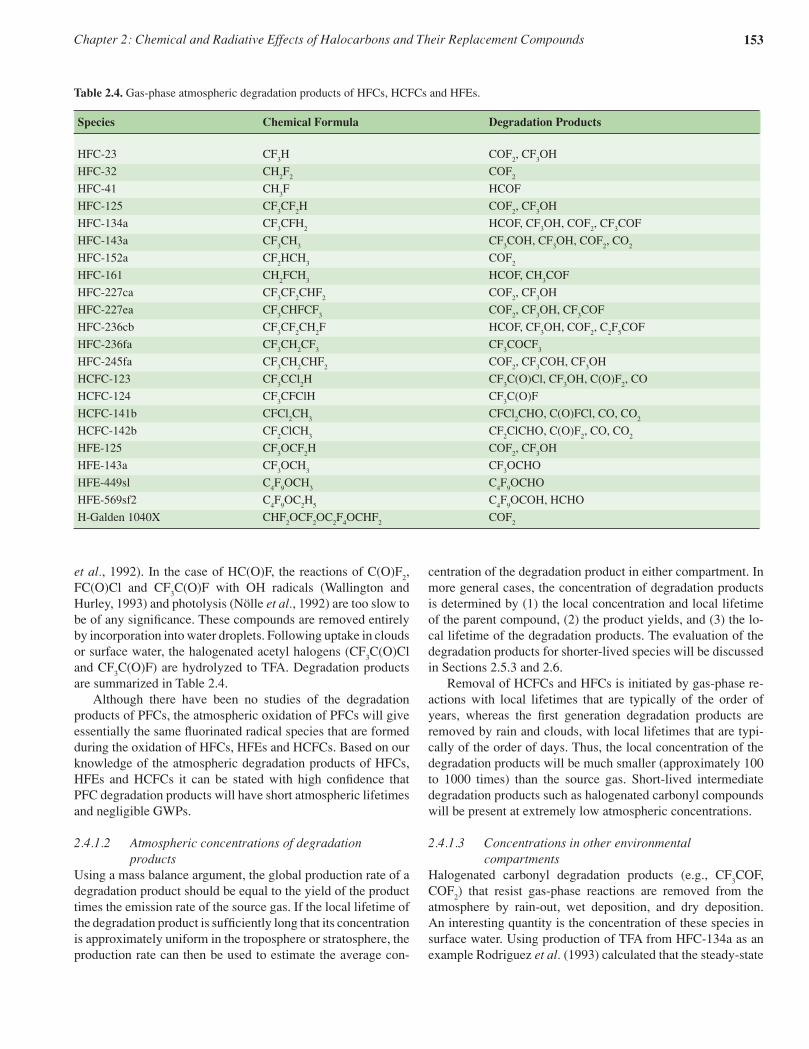
Chapter 2: Chemical and Radiative Effects of Halocarbons and Their Replacement Compounds 153
et al., 1992). In the case of HC(O)F, the reactions of C(O)F2,
FC(O)Cl and CF3C(O)F with OH radicals (Wallington and
Hurley, 1993) and photolysis (Nölle et al., 1992) are too slow to be of any significance. These compounds are removed entirely by incorporation into water droplets. Following uptake in clouds or surface water, the halogenated acetyl halogens (CF
3C(O)Cl
and CF3C(O)F) are hydrolyzed to TFA. Degradation products
are summarized in Table 2.4. Although there have been no studies of the degradation products of PFCs, the atmospheric oxidation of PFCs will give essentially the same fluorinated radical species that are formed during the oxidation of HFCs, HFEs and HCFCs. Based on our knowledge of the atmospheric degradation products of HFCs, HFEs and HCFCs it can be stated with high confidence that PFC degradation products will have short atmospheric lifetimes and negligible GWPs.
2.4.1.2 Atmospheric concentrations of degradation products
Using a mass balance argument, the global production rate of a degradation product should be equal to the yield of the product times the emission rate of the source gas. If the local lifetime of the degradation product is sufficiently long that its concentration is approximately uniform in the troposphere or stratosphere, the production rate can then be used to estimate the average con-
centration of the degradation product in either compartment. In more general cases, the concentration of degradation products is determined by (1) the local concentration and local lifetime of the parent compound, (2) the product yields, and (3) the lo-cal lifetime of the degradation products. The evaluation of the degradation products for shorter-lived species will be discussed in Sections 2.5.3 and 2.6. Removal of HCFCs and HFCs is initiated by gas-phase re-actions with local lifetimes that are typically of the order of years, whereas the first generation degradation products are removed by rain and clouds, with local lifetimes that are typi-cally of the order of days. Thus, the local concentration of the degradation products will be much smaller (approximately 100 to 1000 times) than the source gas. Short-lived intermediate degradation products such as halogenated carbonyl compounds will be present at extremely low atmospheric concentrations.
2.4.1.3 Concentrations in other environmental compartments
Halogenated carbonyl degradation products (e.g., CF3COF,
COF2) that resist gas-phase reactions are removed from the
atmosphere by rain-out, wet deposition, and dry deposition. An interesting quantity is the concentration of these species in surface water. Using production of TFA from HFC-134a as an example Rodriguez et al. (1993) calculated that the steady-state
Table 2.4. Gas-phase atmospheric degradation products of HFCs, HCFCs and HFEs.
Species Chemical Formula Degradation Products
HFC-23 CF3H COF
2, CF
3OH
HFC-32 CH2F
2 COF
2
HFC-41 CH3F HCOF
HFC-125 CF3CF
2H COF
2, CF
3OH
HFC-134a CF3CFH
2 HCOF, CF
3OH, COF
2, CF
3COF
HFC-143a CF3CH
3 CF
3COH, CF
3OH, COF
2, CO
2
HFC-152a CF2HCH
3 COF
2
HFC-161 CH2FCH
3 HCOF, CH
3COF
HFC-227ca CF3CF
2CHF
2 COF
2, CF
3OH
HFC-227ea CF3CHFCF
3 COF
2, CF
3OH, CF
3COF
HFC-236cb CF3CF
2CH
2F HCOF, CF
3OH, COF
2, C
2F
5COF
HFC-236fa CF3CH
2CF
3 CF
3COCF
3
HFC-245fa CF3CH
2CHF
2 COF
2, CF
3COH, CF
3OH
HCFC-123 CF3CCl
2H CF
3C(O)Cl, CF
3OH, C(O)F
2, CO
HCFC-124 CF3CFClH CF
3C(O)F
HCFC-141b CFCl2CH
3 CFCl
2CHO, C(O)FCl, CO, CO
2
HCFC-142b CF2ClCH
3 CF
2ClCHO, C(O)F
2, CO, CO
2
HFE-125 CF3OCF
2H COF
2, CF
3OH
HFE-143a CF3OCH
3 CF
3OCHO
HFE-449sl C4F
9OCH
3 C
4F
9OCHO
HFE-569sf2 C4F
9OC
2H
5 C
4F
9OCOH, HCHO
H-Galden 1040X CHF2OCF
2OC
2F
4OCHF
2 COF
2
IPCC Boek (dik).indb 153 15-08-2005 10:53:54

154 IPCC/TEAP Special Report: Safeguarding the Ozone Layer and the Global Climate System
global averaged rain-water concentration of TFA is of the order of 1 µg L–1 for an annual emission of 1000 kt yr–1 of HFC-134a. Subsequent calculations using a 3-D model (Kotamarthi et al., 1998) showed that the local rain-water concentration averaged over 10-degree latitude and longitude bands would typically deviate from the global average number by a factor of two. Variation can be much larger on a local scale.
2.4.2 Trifluoroacetic acid (TFA, CF3C(O)OH))
TFA is produced during the atmospheric degradation of several CFC replacements, and partitions into the aqueous compart-ments of the environment (Bowden et al., 1996). Reaction with OH radicals in the gas phase accounts for 10–20% of the loss of TFA (Møgelberg et al., 1994). The major fate of TFA is rain-out. The environmental impact of TFA has been studied thoroughly and results have been reviewed in the UNEP effects-assessment reports of 1998 (Tang et al., 1998) and 2002 (Solomon et al., 2003). TFA is highly soluble in water, is a strong acid with Pka of 0.23 and the logarithm of its n-octanol/water partition coef-ficient is –0.2, which indicates that it will essentially partition in the water compartment and will not bioaccumulate in animals. Little accumulation (concentration factor of approximately 10) occurs in plants exposed to TFA. In a long-term study (90 weeks) (Kim et al., 2000) it was shown that TFA could be biodegraded in an engineered anaerobic waste-water treatment system at a TFA concentration up to 30 mg L–1 (as fluoride). However, it is unclear how this result should be extrapolated to natural en-vironments, where concentrations of TFA and nutrients will be different. Ellis et al. (2001) observed no significant degrada-tion during a 1-year mesocosm study. In the water compartment no significant abiotic degradation process has been identified (Boutonnet et al., 1999). TFA is a persistent substance. Aquatic ecotoxicity studies showed that the most sensitive standard algae species was the algae Selenastrum capricornutum with a no-effect concentration of 0.10 mg L–1 (0.12 mg L–1 for the sodium salt NaTFA) (Berends et al., 1999). Thus, TFA con-
centrations approaching a milligram per litre may be toxic to some aquatic life forms. The TFA concentration in rain water resulting from HFC and HCFC degradation for the year 2010 is expected to be approximately 100 to 160 ng L–1 (Kotamarthi et al., 1998), which is approximately 1000 times smaller than the no-observed-effect concentration of S. Capricornutum. This result and the absence of significant bioaccumulation in biota indicate that no adverse effect on the environment is expected (Tang et al., 1998; Solomon et al., 2003). TFA is not metabo-lized in mammalian systems. Toxicity studies indicate that TFA will have biological effects similar to other strong acids (Tang et al., 1998). In conclusion, no adverse effects on human or ecosystem health are expected from the TFA produced by at-mospheric degradation of CFC substitutes. Atmospheric concentrations of HFC-134a, HCFC-124, and HCFC-123 have been measured at 25.5 ppt, 1.34 ppt, and 0.03 ppt, respectively (see Table 2.1). The corresponding atmospher-ic burdens are 439.0 kt, 30.84 kt, and 0.774 kt, respectively. Degradation fluxes can be calculated using lifetime values from WMO (2003) and TFA yields, and TFA fluxes can be calculated at 10,266 t yr –1 of TFA for the year 2000 (Table 2.5). TFA has been observed in varying concentrations in surface waters (oceans, rivers and lakes) and in fog, snow and rain-water samples around the globe, for example, in the USA, Germany, Israel, Ireland, France, Switzerland, Austria, Russia, South Africa and Finland (see references in Nielsen et al., 2001). TFA appears to be a ubiquitous component of the contemporary hydrosphere. TFA is reported in concentrations of about 200 ng L–1 in ocean water down to depths of several thousand meters (Frank et al., 2002). If 200 ng L–1 is the average concentration of TFA in all ocean water, the oceans contain around 3 × 10⁸ t of TFA. With an anthropogenic contribution of 10,266 t yr–1 it would have taken approximately 3400 years to achieve the present TFA concentra-tion in ocean waters; therefore, industrial sources cannot explain the observed abundance of TFA in ocean water. High TFA con-centrations in the Dead Sea and Nevada lakes, of 6400 ng L–1 and 40,000 ng L–1, respectively, suggest long-term accumula-
Table 2.5. Sources of TFA.
Species Chemical Formula Molar Yield of Lifetime Global TFA TFA (yr) Production (t yr–1)
Halothane CF3CHClBr 0.6 1.2 520a
Isoflurane CF3CHClOCHF
2 0.6 5 280a
HCFC-123 CF3CHCl2 0.6 1.3 266b
HCFC-124 CF3CHFCl 1.0 5.8 4440b
HFC-134a CF3CH
2F 0.13 14 4560b
Fluoropolymers 200c
TFA (lab use etc) NegligibleTotal 10,266
a Tang et al. (1998).b Based on the atmospheric burden derived from data in Table 2.1.c Jordan and Frank (1999).
IPCC Boek (dik).indb 154 15-08-2005 10:53:55

Chapter 2: Chemical and Radiative Effects of Halocarbons and Their Replacement Compounds 155
tion over centuries and the existence of pre-industrial sources of TFA (Boutonnet et al., 1999). However, TFA was not found in pre-industrial (>2000 years old) fresh water taken from Greenland and Denmark (Nielsen et al., 2001). Therefore, although it ap-pears that there is a significant natural source of TFA, the identity of this source is unknown. Because of the persistence of TFA, it has been suggested that it could accumulate in aquatic ecosystems like vernal pools or seasonal wetlands, which dry out periodically, are replenished by rainfall and are presumed to have little or no seepage (Tromp et al., 1995). A sensitivity study (Tromp et al., 1995) based on mathematical modelling suggested that such accumulation could take place if a series of conditions (a polluted area with high atmospheric concentrations of the precursors and the OH radical; pollution and rainfall events that occur at the same time; and little, or no, seepage) could be maintained simultaneously for several decades. An example cited by the authors indicated that if the concentration of TFA in rain water was assumed to be 1 µg L–1, and the loss frequencies were 5 yr–1 for evaporation and of 0.1 yr–1 for seepage, the TFA concentration could reach 100 µg L–1 (which corresponds to the no-effect concentration of the most sensitive aquatic species) in 30 years. The probability that such a combination of events would be maintained over several decades appears to be rather low (Solomon et al., 2003). Studies of pond water (Tang et al., 1998) confirmed TFA’s per-sistent behaviour but did not find significant accumulation. TFA evapoconcentration was observed during two years in 1998 and 1999 in vernal pools in California (Cahill et al., 2001). Some TFA retention was also observed between the years 1998 and 1999 but was not easily quantified. Cahill et al. (2001) sug-gested that in very wet years surface-water export may occur and may limit long-term TFA accumulation. Concentrations ob-served at the beginning of the study in January 1998 were about 130 ng L–1 (in the range of expected rain-water concentrations) and suggest that accumulation was not maintained in previous years. Although some accumulation is likely in such systems because of TFA persistence, observations indicate that the spe-cific conditions required for accumulation in seasonal wetlands are unlikely to be maintained for several decades.
2.4.3 Other halogenated acids in the environment
Long-chain perfluorinated carboxylic acids (PFCAs, CnF2n+1
COOH, where n = 6–12) have been observed in biota, and in surface and ground water (Moody and Field, 1999; Moody et al., 2001; Moody et al., 2002; Martin et al., 2004). These PFCAs have no known natural sources, are bioaccumula-tive, and have no known loss mechanisms in the environment. The health effects from exposure to perfluorooctanoic acid are the subject of a present risk assessment (US EPA, 2003). PFCAs are not generally used directly in industrial mate-rials or consumer products. The observation of PFCAs in re-mote locations presumably reflects their formation as degra-dation products of precursor chemicals in the atmosphere. It has been suggested that degradation of fluorotelomer alcohols,
F(CF2CF
2)
nCH
2CH
2OH (n = 3–6), is a likely source of PFCAs
observed in remote locations (Andersen et al., 2003; Ellis et al., 2004), but the importance of this source is unclear. Further studies are needed to quantify the sources of PFCAs in the en-vironment. HFCs, HCFCs and HFEs used as CFC replacements generally have short-chain fluorinated alkyl substituents and so will not contribute to long-chain PFCA pollution. Several haloacetic acids (HAA) have been detected in en-vironmental samples. Besides TFA, monochloroacetic acid (MCA), dichloroacetic acid (DCA), and trichloroacetic acid (TCA) (Scott et al., 2000) and chlorodifluoroacetic acid (CDFA) (Martin et al., 2000) have been measured in, for example, rain, snow and lake samples. The contribution of HCFCs to chlo-rofluoro-substituted carboxylic acids is unclear.
2.4.4 Ammonia (NH3)
It is widely recognized that the bulk of the atmospheric emis-sions of ammonia (NH
3) is removed from the atmosphere by
dry and wet deposition processes and by reaction with strong acids to form ammonium compounds. The latter are important aerosol components with direct and indirect effects on radiative forcing. Some of the NH
3 emitted at the surface survives and is
carried into the free troposphere above the atmospheric bound-ary layer. There, the main removal process for NH
3 is by the
reaction with hydroxyl OH radicals:
OH + NH3 → H
2O + NH
2 [2.3]
The lifetime of NH3 in the troposphere attributed to Reaction
[2.3] has been estimated to range from 72 to 109 days (Finlayson-Pitts and Pitts, 2000; Warneck, 1999). The main re-action product of NH
3 degradation is the amidogen NH
2 radical,
whose main fate is to react with NOx and ozone and thereby act
as a source or a sink for NOx and as a source of nitrous oxide
(N2O), which is a long-lived well-mixed greenhouse gas:
NH2 + NO → N
2 + H
2O [2.4]
NH2 + NO
2 → N
2O + H
2O [2.5]
NH2 + O
3 → NH
2O + O
2 [2.6]
In a 3-D chemistry-transport model study, Dentener and Crutzen (1994) suggested that the degradation of NH
3 may generate up
to about 1 TgN yr–1 of N2O from a global NH
3 source strength
of 45 Tg yr–1. It should be noted that 1 TgN yr–1 of N2O would
represent about 6% of the global source strength of N2O (as N)
inferred by IPCC (2001, Chapter 4). However, because there is some question whether Reaction [2.5] occurs in the atmosphere as written here, the conversion of NH
3 to N
2O may be much
smaller (Warneck, 1999).
IPCC Boek (dik).indb 155 15-08-2005 10:53:55

156 IPCC/TEAP Special Report: Safeguarding the Ozone Layer and the Global Climate System
2.5 Radiative properties and global warming potentials
Halocarbons released into the atmosphere can affect climate in several ways. These molecules mostly absorb radiation in a spectral window region of the outgoing thermal longwave radiation (see Figure 2.6) and hence are efficient greenhouse gases. Halocarbons can also have indirect effects on climate by causing destruction of ozone (see Chapter 1) or through altera-tions to tropospheric chemistry (see Section 2.5.3). Global climate models are the tools that are used to under-stand and predict how current and future human emissions of halocarbons contribute to climate forcing. The concepts of radi-ative forcing and global warming potential (GWP) (see Box 2.2 for definitions) were introduced in 1990 (IPCC, 1990; Fisher et al., 1990). They are still widely used as convenient ways to
compare and quantify the relative contribution of equal-mass emissions of different gases to climate forcing, even if it is ac-knowledged that the use of these simplified formulations has its limitations. Recent publications highlight that different calcula-tions are possible to derive radiative forcings (Hansen et al., 2002; Gregory et al., 2004) and that other possible tools can be constructed to compare the climate impacts of greenhouse gases (Shine et al., 2003; Shine et al., 2005).
2.5.1 Calculation of GWPs
The contribution of a gas to the warming of the atmosphere is a function of its ability to absorb the longwave infrared radiation over a specified period of time, which in turn depends on its concentration, atmospheric steady-state lifetime, and infrared absorption properties (see Figure 2.7).
� � � �� �� �� ���
��
��
��
��
���
���
����
����
���
����������������������
� � � �� �� �� ���
�
�
�
�
�
���������������������
���������������
���
����
�����
����
�� �
���
����
����
����
� �
������������������������������
���
��� ���
��� ��
���
Figure 2.6. Top panel: Atmospheric absorption of infrared radiation (0 is for no absorption and 100% is for full absorption) as derived from the space-borne IMG/ADEOS radiance measurements (3 April 1997; 9.5°W, 38.4°N). Bottom panel: Halocarbons (HCFC-22, CFC-12, HFC-134a) absorption cross-sections in the infrared atmospheric window, which lies between the nearly opaque regions caused by strong absorption by CO
2,
H2O, O
3, CH
4 and N
2O.
IPCC Boek (dik).indb 156 15-08-2005 10:53:57

Chapter 2: Chemical and Radiative Effects of Halocarbons and Their Replacement Compounds 157
The direct GWP of a gas x is calculated as the ratio of the time-integrated radiative forcing from a pulse emission of 1 kg of that gas relative to that of 1 kg of a reference gas
(2.5)
where TH is the integration time (the time horizon) over which the calculation is performed. The gas chosen as reference is generally CO
2, although its atmospheric decay function is sub-
ject to substantial scientific uncertainties (IPCC, 1994). The numerator of Equation (2.5) is the absolute GWP (AGWP) of a gas. In practice, the AGWP is calculated using
the following procedure:
(2.6)
where, ax is the radiative forcing due to a unit mass increase of the gas x distributed according to its expected steady-state distribution for continuous emission, ΔBx(t) is the change in burden due to the pulse emission, and τx is the lifetime of the perturbation of species x. The calculation is performed over a finite period of time to facilitate policy considerations. The integration time ranges from 20 to 50 years if atmospheric response (e.g., surface tem-perature change) is of interest, or from 100 to 500 years if a long-term effect (such as sea-level rise) is to be considered. Substances with very long lifetimes, such as PFCs and SF
6, have contributions that may exceed these time scales, and
hence the use of GWP may be inadequate for these species. Conversely, one should be cautious about using the derived GWP values for gases with lifetimes shorter than 5 years that may not be uniformly mixed in the atmosphere, although the concept may be used to some extent for short-lived species and can be applied to the calculation of indirect contributions as ad-dressed in Section 2.5.3.
2.5.2 Calculation of radiative forcing
The radiative forcing due to a change in the abundance of a greenhouse gas is the net (down minus up) irradiance change (in watts per square meter, W m–2) at the tropopause induced by this perturbation. It is calculated using a forward radiative-trans-fer code that computes the irradiance at different atmospheric levels, with the infrared absorption spectrum of the molecule as a key input. Calculation can be performed using simplified as-sumptions (clear-sky instantaneous forcings) or using improved schemes that take into account cloud coverage and allow strat-ospheric temperatures to re-adjust to radiative equilibrium (ad-
Box 2.2. Definitions of radiative forcing and global warming potential (GWP)
Radiative forcing• The radiative forcing quantifies the ability of a gas to perturb the Earth’s radiative energy budget.• Definition: The radiative forcing of the surface-troposphere system due to the perturbation in or the introduction of gas
is the change in net (down minus up) irradiance (solar plus longwave, in W m–2) at the tropopause, after allowing for stratospheric temperatures to re-adjust to radiative equilibrium, but with surface and tropospheric temperatures and other state variables (clouds, water) held fixed at the unperturbed values.
Global warming potential (GWP)• The global warming potential is a relative index used to compare the climate impact of an emitted greenhouse gas, relative
to an equal amount of carbon dioxide.• Definition: The global warming potential is the ratio of the time-integrated radiative forcing from a pulse emission of 1 kg
of a substance, relative to that of 1 kg of carbon dioxide, over a fixed horizon period.
�����������
��������
������
���
���
���
�����������������������������
���
�����
���
����
����
����
����
�����
���
����
�
����
����
����
����
����
����
����
����
���������� ������ ������
� �� ��� �����������������������������������
Figure 2.7. The time evolution of the radiative forcing (in W m–2) associated with the decay of a pulse emission, released into the atmosphere at time t = 0, of various gases with an atmospheric lifetime spanning 1.4 years (HFC-152a) to 50,000 years (CF4) (see also Figure 2.2). The 20-, 100-, and 500-year time horizons (TH) used for GWP calculations are shown by vertical lines.
IPCC Boek (dik).indb 157 15-08-2005 10:54:05

158 IPCC/TEAP Special Report: Safeguarding the Ozone Layer and the Global Climate System
justed cloud forcings). Because of the current low abundances of the halocarbons in the atmosphere, their radiative forcing is proportional to their atmospheric abundance. This is to be con-trasted with abundant gases, such as CO
2, for which the effect
is nonlinear because of saturation of absorption. Halocarbons exhibit strong absorption bands in the thermal infrared atmospheric window (see Figure 2.6) because of their various vibrational modes. Absorption spectra of CFCs and the majority of proposed substitutes are characterized by absorp-tion bands rather than lines, because individual spectral lines for these heavy molecules are overlapping and not resolved at tropospheric pressures and temperatures. For each gas, the ab-sorption cross-sections (in cm2 per molecule) are derived from laboratory measurements for specific atmospheric conditions. Several independent measurements of absorption cross-sec-tions for halocarbons have been reported in the literature (e.g., McDaniel et al., 1991; Clerbaux et al., 1993; Clerbaux and Colin, 1994; Varanasi et al., 1994; Pinnock et al., 1995; Barry et al., 1997; Christidis et al., 1997, Ko et al., 1999; Sihra et al., 2001; Orkin et al., 2003; Nemtchinov and Varanasi, 2004; Hurley et al., 20051) and some of these data sets are available through the widely used molecular spectroscopic databases, such as HITRAN (Rothman et al., 2003) and GEISA (Jacquinet-Husson et al., 1999). The intercomparison of measured cross-sections and integrated absorption intensities performed on the same molecule by different groups provides an estimate of the discrepancies among the obtained results, and hence of the measurement accuracy (e.g., Ballard et al., 2000; Forster et al., 2005). Although the discrepancies between different cross-section measurements can reach 40% (Hurley et al., 2005), it is recognized that the typical uncertainties associated with the measured cross-section when integrated over the infrared spec-tral range are less than 10%. The measured spectroscopic data are then implemented into a radiative transfer model to compute the radiative fluxes. Several radiative-transfer models are available, ranging from line-by-line to wide-bands models, depending on the spectral interval over which the calculation is performed. Apart from the uncertainties stemming from the cross-sections themselves, differences in the flux calculation can arise from the spectral resolution used; tropopause heights; vertical, spatial and sea-sonal distributions of the gases; cloud cover; and how strat-ospheric temperature adjustments are performed. The impact of these parameters on radiative forcing calculations is discussed in comprehensive studies such as Christidis et al. (1997), Hansen et al. (1997), Myhre and Stordal (1997), Freckleton et al. (1998), Highwood and Shine (2000), Naik et al. (2000), Jain et al. (2000), Sihra et al. (2001) and Forster et al. (2005). The discrepancy in the radiative forcing calculation for differ-ent halocarbons, which is associated with different assumptions used in the radiative transfer calculation or with use of different
cross-section sets, can reach 40% (Gohar et al., 2004). Recent studies performed for the more abundant HFCs (HFC-23, HFC-32, HFC-134a and HFC-227ea) report that an agreement better than 12% can be reached when the calculation conditions are better constrained (Gohar et al., 2004; Forster et al., 2005). Recommended radiative forcings and associated GWP val-ues, gathered from previous reports and recently published data, are provided in Section 2.5.4.
2.5.3 Other aspects affecting GWP calculations
The discussion in the preceding sections describes methods to evaluate the direct radiative impact of emission of a source gas that has a sufficiently long lifetime so that it has a uniform mix-ing ratio in the troposphere. This section considers two aspects of GWP calculations that are not covered by these methods. First, the direct impact refers only to the greenhouse warming arising from the accumulation of the source gas in the atmos-phere, but does not consider its other radiatively important byproducts. There could be indirect effects if the degradation products of the gas also behaved like greenhouse gases (Section 2.5.3.1), or if the presence of the emitted gas and its degradation products affected the distribution of other greenhouse gases (Section 2.5.3.2). Second, the special case of very short-lived source gases with non-uniform mixing ratios in the troposphere will be discussed (Section 2.5.3.3).
2.5.3.1 Direct effects from decomposition productsThe indirect radiative effects of the source gas include the di-rect effects from its degradation products. As was discussed in Section 2.4.1 the local concentrations of most degradation prod-ucts, with very few exceptions, are a factor of 100 (or more) smaller than that of the source gas. Assuming that the values for the radiative forcing of the source gas and its degradation prod-ucts are similar, the indirect GWP from the degradation prod-ucts should be much smaller than the direct GWP of the source gas except for cases where the local lifetime of the degradation product is longer than that of the source gas. CO
2 is one of the
final degradation products of organic compounds. However the magnitude of the indirect GWP attributed to CO
2 is equal to the
number of carbons atoms in the original molecule, and is small compared with the direct GWP values of most of the halocar-bons given in Table 2.6.
2.5.3.2 Indirect effects from influences on other atmospheric constituents
As discussed in Chapter 1, chlorine and bromine atoms released by halocarbons deplete ozone in the stratosphere. Because ozone is a greenhouse gas, its depletion leads to cooling of the climate system. This cooling is a key indirect effect of halo-carbons on radiative forcing and is particularly significant for gases containing bromine. Daniel et al. (1995) described a method for characterizing the net radiative forcing from halocarbons emitted in the year 1990. Although the method and the values are often discussed
1 This most recently published work was not available in time to be fully con-sidered by the authors.
IPCC Boek (dik).indb 158 15-08-2005 10:54:11

Chapter 2: Chemical and Radiative Effects of Halocarbons and Their Replacement Compounds 159
in the context of net GWP, it was clearly explained in Daniel et al. (1995) that they differ from direct GWP in the following ways:1. The net GWP is most useful for comparing the relative
radiative effects of different ODSs when emitted at the same time. In the type of calculations that may be performed in the following chapters, one may come across a situation where the GWP weighted emissions from several well-mixed greenhouse gases and ODSs add to zero. It is important to recognize that the result does not guarantee zero climate impact.
2. The amount of ozone depletion caused by an incremental emission of an ODS depends on the equivalent effective stratospheric chlorine (EESC) loading in the atmosphere. The concept of EESC has long been used to assess the effect of halocarbon emissions on the ozone-depleting effect of halogens in the stratosphere (Prather and Watson, 1990; Chapter 1 of WMO, 2003 and references therein; and Figure 1.18 in Chapter 1 of this report). Ozone depletion first began to be observable around 1980, and the date when EESC is projected to fall below its 1980 value can provide a rough estimate of the effects of emissions on the time scale for ozone recovery, assuming no changes in other parameters, such as atmospheric circulation or chemical composition. Chapter 1 of this report assesses in detail the factors that are likely to influence the date of ozone recovery, intercompares model estimates of the date, and discusses uncertainties in its absolute value. EESC is used here to indicate the relative effect of several different future emission scenarios on the date of ozone recovery, but not to identify the absolute value of the date. Current projections based on emission scenarios indicate that the threshold values for EESC will be achieved between 2043 and 2046, when there will be no further ozone depletion for incremental ODS emission. Because the indirect forcing of ODSs becomes zero after the EESC threshold is reached, indirect GWPs for emissions prior to that time decrease as they occur closer to the recovery threshold. Indirect GWPs for emissions that occur after the threshold is reached are zero.
The method described in Daniel et al. (1995) assumes an EESC-loading curve for the future based on an emission scenario in compliance with the Montreal Protocol and its subsequent up-dates. Values given in Daniel et al. (1995) are for several emis-sion scenarios (future EESC curves) appropriate for emissions in 1990. Subsequent updates in IPCC (1994), WMO (1999) and IPCC (2001) use a single emission scenario for 1990 emis-sion. The values in WMO (2003) are for an emission in the year 2002. HCFCs, HFCs and some of their replacement gases (hydro-carbons and ammonia) also have the potential to alter the ra-diative balance in the atmosphere indirectly by influencing the sources or sinks of greenhouse gases and aerosols. Oxidation by hydroxyl (OH) radicals in the troposphere is the main removal process for the organic compounds emitted by human activi-
ties. This oxidation acts as a source of ozone and as a removal process for hydroxyl radicals, thereby reducing the efficiency of methane oxidation and promoting the build-up of methane. Therefore, emissions of organic compounds, including HCFCs, HFCs and some of their replacement gases, may lead to the build-up of two important greenhouse trace gases, methane and ozone, and consequently may cause an indirect radiative forc-ing (e.g., Lelieveld et al., 1998; Johnson and Derwent, 1996; Fuglestvedt et al., 1999). The main factors influencing the magnitudes of such indirect radiative impacts were found to be their spatial emission patterns, chemical reactivity and trans-port, molecular complexity, and the oxidation products formed (Collins et al., 2002). Another possible indirect effect may result from the reac-tion of the degradation products of HCFCs and HFCs with OH or O
3, which may modify the OH or O
3 distributions. However,
it is unlikely that degradation products of the long-lived HCFCs and HFCs have a large impact on a global scale, because the effect would occur after the emission is distributed around the globe, which will result in relatively low concentrations.
2.5.3.3 Very short-lived hydrocarbonsAssigning GWP values to very short-lived (VSL) species (spe-cies with a lifetime of a month or shorter) presents a special challenge (WMO, 2003, Chapter 2). Because of their short life-times VSL species are not uniformly distributed in the tropo-sphere. Their distributions depend on where and when (during the year) they are emitted. Thus, it is not possible to assign a single steady-state change in burden in the troposphere per unit mass emission. In calculating the local change in radiative forcing, one would have to use their actual three-dimensional distributions. Furthermore, it is not obvious how one would es-timate the change in surface temperature from the local changes in forcing. In a sense, the issue is similar to the situation for aerosol forcing. In such cases, the notion of GWP may prove less useful and one would have to examine the local climate impact directly, along with other indirect effects, such as ozone and aerosol formation. Given the infrared absorption cross-section of a VSL spe-cies, it is possible to use current tools to compute a local ra-diative forcing per unit burden change for a local column. This value can be used to obtain estimates for a GWP-like quantity by examining the decay rate of a pulse emission. In most cases this value will be small compared with the GWP value of the long-lived HCFCs and HFCs, and may indicate that the glo-bal impact from VSL species used as halocarbon substitutes is small. However, it is not clear how such forcing may produce impacts on a smaller (e.g., regional) scale.
2.5.4 Reported values
The lifetimes, the radiative efficiencies (radiative forcing per concentration unit) and the GWPs of the substances controlled by the Montreal Protocol and of their replacements are given in Table 2.6. The GWP for a gas is the ratio of the absolute global
IPCC Boek (dik).indb 159 15-08-2005 10:54:11

160 IPCC/TEAP Special Report: Safeguarding the Ozone Layer and the Global Climate SystemTa
ble
2.6.
Lif
etim
es, r
adia
tive
effic
ienc
ies,
and
dir
ect g
loba
l war
min
g po
tent
ials
(G
WPs
) re
lativ
e to
car
bon
diox
ide,
for
the
OD
Ss a
nd th
eir
repl
acem
ents
.
Ind
ustr
ial D
esig
nati
on
Che
mic
al F
orm
ula
Oth
er N
ame
L
ifet
imea
Rad
iati
ve
Glo
bal W
arm
ing
Pot
enti
al fo
r a
Giv
en T
ime
Hor
izon
or
Com
mon
Nam
e
(y
r)
Effi
cien
cya
IPC
C (1
996)
b
IPC
C (2
001)
& W
MO
(200
3)
(W m
–2 p
pb–1
) 10
0 yr
20
yr
100
yr
500
yr
Car
bon
diox
ide
CO
2
Se
e te
xt
1 1
1 1
Met
hane
C
H4
12
.0c
3.7
× 1
0–4
21
63c
23c
7c
Sub
stan
ces
cont
rolle
d by
the
Mon
trea
l Pro
toco
l
CFC
-11
CC
l 3F
Tri
chlo
roflu
orom
etha
ne
45
0.25
38
00
6330
46
80
1630
CFC
-12
CC
l 2F2
Dic
hlor
odifl
uoro
met
hane
10
0 0.
32
8100
10
,340
10
,720
52
30C
FC-1
13
CC
l 2FC
ClF
2 1,
1,2-
Tri
chlo
rotr
ifluo
roet
hane
85
0.
3 48
00
6150
60
30
2700
CFC
-114
C
ClF
2CC
lF2
Dic
hlor
otet
raflu
oroe
than
e 30
0 0.
31
75
60
9880
87
80C
FC-1
15
CC
lF2C
F 3 M
onoc
hlor
open
taflu
oroe
than
e 17
00
0.18
4990
72
50
10,0
40H
alon
-130
1 C
BrF
3 B
rom
otri
chlo
roet
hane
65
0.
32
5400
79
70
7030
27
80H
alon
-121
1 C
BrC
lF2
Bro
moc
hlor
odifl
uoro
etha
ne
16d
0.3
44
60
1860
57
8H
alon
-240
2 C
BrF
2CB
rF2
Dib
rom
otet
raflu
oroe
than
e 20
d 0.
33d
34
60d
1620
d 50
5d
Car
bon
tetr
achl
orid
e C
Cl 4
26
d 0.
13
1400
25
40d
1380
d 43
7d
Met
hyl b
rom
ide
CH
3Br
0.
7 0.
01
16
5
1B
rom
ochl
orom
etha
ne
CH
2BrC
l
0.37
d
M
ethy
l chl
orof
orm
C
H3C
Cl 3
1,1,
1-T
rich
loro
etha
ne
5.0d
0.06
476d
144d
45d
HC
FC-2
2 C
HC
lF2
Chl
orod
ifluo
rom
etha
ne
12d
0.20
15
00
4850
d 17
80d
552d
HC
FC-1
23
CH
Cl 2C
F 3 D
ichl
orot
riflu
oroe
than
e 1.
3d 0.
14d
90
257d
76d
24d
HC
FC-1
24
CH
ClF
CF 3
Chl
orot
etra
fluor
oeth
ane
5.8d
0.22
47
0 19
50d
599d
186d
HC
FC-1
41b
CH
3CC
l 2F
Dic
hlor
ofluo
roet
hane
9.
3 0.
14
21
20
713
222
HC
FC-1
42b
CH
3CC
lF2
Chl
orod
ifluo
roet
hane
17
.9c
0.2
1800
51
70
2270
70
9H
CFC
-225
ca
CH
Cl 2C
F 2CF 3
Dic
hlor
open
taflu
orop
ropa
ne
1.9d
0.2d
40
4d 12
0d 37
d
HC
FC-2
25cb
C
HC
lFC
F 2CC
lF2
Dic
hlor
open
taflu
orop
ropa
ne
5.8d
0.32
1910
d 58
6d 18
2d
Hyd
roflu
oroc
arbo
ns
H
FC-2
3 C
HF 3
Tri
fluor
omet
hane
27
0d 0.
19e
11,7
00
11,1
00f
14,3
10f
12,1
00f
HFC
-32
CH
2F2
Difl
uoro
met
hane
4.
9d 0.
11e
650
2220
f 67
0f 21
0f
HFC
-125
C
HF 2C
F 3 Pe
ntafl
uoro
etha
ne
29
0.23
28
00
5970
34
50
1110
HFC
-134
a C
H2F
CF 3
1,1,
1,2-
Tetr
afluo
roet
hane
14
d 0.
16e
1300
35
90f
1410
f 44
0f
HFC
-143
a C
H3C
F 3 1,
1,1-
Tri
fluor
oeth
ane
52
0.13
38
00
5540
44
00
1600
HFC
-152
a C
H3C
HF 2
1,1-
Difl
uoro
etha
ne
1.4
0.09
14
0 41
1 12
2 38
HFC
-227
ea
CF 3C
HFC
F 3 1,
1,1,
2,3,
3,3-
Hep
taflu
orop
ropa
ne
34.2
d 0.
26e
2900
49
30f
3140
f 10
30f
HFC
-236
fa
CF 3C
H2C
F 3 1,
1,1,
3,3,
3-H
exafl
uoro
prop
ane
240d
0.28
63
00
7620
d 95
00d
7700
d
HFC
-245
fa
CH
F 2CH
2CF 3
1,1,
1,3,
3-Pe
ntafl
uoro
prop
ane
7.6d
0.28
3180
d 10
20d
316d
HFC
-365
mfc
C
H3C
F 2CH
2CF 3
1,1,
1,3,
3-Pe
ntafl
uoro
buta
ne
8.6d
0.21
2370
d 78
2d 24
3d
HFC
-43-
10m
ee
CF 3C
HFC
HFC
F 2CF 3
1,1,
1,2,
3,4,
4,5,
5,5-
Dec
afluo
rope
ntan
e 15
.9d
0.4
1300
38
90d
1610
d 50
2d
Per
fluor
inat
ed c
ompo
unds
Su
lphu
r he
xaflu
orid
e SF
6
3200
0.
52
23,9
00
15,2
90
22,4
50
32,7
80N
itrog
en tr
ifluo
ride
N
F 3
740
0.13
7780
10
,970
13
,240
PFC
-14
CF 4
Car
bon
tetr
afluo
ride
50
,000
0.
08
6500
39
20
5820
90
00PF
C-1
16
C2F
6 Pe
rfluo
roet
hane
10
,000
0.
26
9200
81
10
12,0
10
18,2
80PF
C-2
18
C3F
8 Pe
rfluo
ropr
opan
e 26
00
0.26
70
00
5940
86
90
12,5
20PF
C-3
18
c-C
4F8
Perfl
uoro
cycl
obut
ane
3200
0.
32
8700
68
70
10,0
90
14,7
40
IPCC Boek (dik).indb 160 15-08-2005 10:54:12

Chapter 2: Chemical and Radiative Effects of Halocarbons and Their Replacement Compounds 161
Tabl
e 2.
6. (
cont
inue
d)
Indu
stri
al D
esig
nati
on
Che
mic
al F
orm
ula
Oth
er N
ame
Lif
etim
ea R
adia
tive
Glo
bal W
arm
ing
Pot
enti
al fo
r a
Giv
en T
ime
Hor
izon
or
Com
mon
Nam
e
(y
r)
Effi
cien
cya
IP
CC
(199
6)b
IP
CC
(200
1) &
WM
O (2
003)
(W
m–2
ppb
–1)
100
yr
20 y
r 10
0 yr
50
0 yr
P
erflu
orin
ated
com
poun
dsPF
C-3
-1-1
0 C
4F10
Pe
rfluo
robu
tane
26
00
0.33
70
00
5950
87
10
12,5
50PF
C-5
-1-1
4 C
6F14
Pe
rfluo
rohe
xane
32
00
0.49
74
00
6230
91
40
13,3
50F
luor
inat
ed e
ther
s
HFE
-449
sl
CH
3O(C
F 2)3C
F 3
5 0.
31
13
10
397
123
HFE
-569
sf2
CH
3CH
2O(C
F 2)3C
F 3
0.77
0.
3
189
56
17H
FE-3
47pc
f2g
CF 3C
H2O
CF 2C
HF 2
7.
1 0.
25
18
00
540
170
Hyd
roca
rbon
s an
d ot
her
com
poun
dsh
E
than
e C
2H6
(R-1
70)
0.21
i 0.
0032
j
Cyc
lopr
opan
e c-
C3H
6 (C
-270
) 0.
44i
Prop
ane
C3H
8 (R
-290
) 0.
041i
0.00
31j
n-
But
ane
CH
3(C
H2)
2CH
3 (R
-600
) 0.
018i
0.00
47j
Is
obut
ane
(CH
3)2C
HC
H3
(R-6
00a)
2-M
ethy
lpro
pane
0.
019i
0.00
47j
Pe
ntan
e C
H3(
CH
2)3C
H3
(R-6
01)
0.01
0i 0.
0046
j
Isop
enta
ne
(CH
3)2C
HC
H2C
H3
(R-6
01a)
2-M
ethy
lbut
ane
0.
010i
Cyc
lope
ntan
e c-
C5H
10
0.
008i
Eth
ylen
e C
H2C
H2
(R-1
150)
Eth
ene
0.
004i
0.03
5j
Prop
ylen
e C
H3C
HC
H2
(R-1
270)
1-P
rope
ne
0.00
1i
A
mm
onia
N
H3
(R-7
17)
a fe
w d
ays
Dim
ethy
leth
er
CH
3OC
H3
0.
015
0.02
1a 1a
<<
1a
Met
hyle
ne c
hlor
ide
CH
2Cl 2
Dic
hlor
omet
hane
0.
38i
0.03
9
35a
10a
3a
Met
hyl c
hlor
ide
CH
3Cl
Chl
orom
etha
ne
1.3
0.01
55a
16a
5a
Eth
yl c
hlor
ide
CH
3CH
2Cl
Chl
oroe
than
e 0.
11d
Met
hyl f
orm
ate
C2H
4O2
0.
16i
Isop
ropa
nol
CH
3CH
OH
CH
3 Is
opro
pyl a
lcoh
ol
0.01
3i
T
rich
loro
ethy
lene
C
Cl 2C
HC
l T
rich
lore
then
e 0.
013i
FK-5
-1-1
2 C
F 3CF 2C
(O)C
F(C
F 3)2
0.
038k
0.3l
n-
Prop
yl b
rom
ide
CH
3CH
2CH
2Br
1-B
rom
opro
pane
, n-P
B
0.04
0.
3l
a Fro
m I
PCC
(20
01, C
hapt
er 6
).b V
alue
s ad
opte
d un
der
the
UN
FCC
C f
or th
e na
tiona
l inv
ento
ries
.c T
he li
fetim
e of
met
hane
incl
udes
fee
dbac
ks o
n em
issi
ons
(IPC
C, 2
001,
Cha
pter
6),
and
GW
Ps in
clud
e in
dire
ct e
ffec
ts (
see
Sect
ion
2.5.
3.2)
.d U
pdat
ed in
WM
O (
2003
, Cha
pter
1).
e Upd
ated
fro
m tw
o av
erag
ed m
odel
res
ults
in G
ohar
et a
l. (2
004)
and
rou
nded
for
con
sist
ency
.f S
cale
d fo
r th
e up
date
d ra
diat
ive
effic
ienc
y no
ted
in (
e).
g Fro
m o
rigi
nal p
aper
by
Toku
hash
i et a
l. (2
000)
. IPC
C (
2001
) er
rone
ousl
y re
ferr
ed to
this
com
poun
ds a
s H
FE-3
74pc
f2.
h Fro
m d
irec
t eff
ects
onl
y. S
ome
valu
es f
or in
dire
ct e
ffec
ts a
re g
iven
in T
able
2.8
.i G
loba
l lif
etim
e es
timat
ed f
rom
a p
roce
ss li
fetim
e, w
ith r
espe
ct to
trop
osph
eric
OH
cal
cula
ted
rela
tive
to 6
.1 y
ears
for
CH
3CC
l 3, as
sum
ing
an a
vera
ge te
mpe
ratu
re o
f 27
2 K
.j H
ighw
ood
et a
l. (1
999)
.k U
pper
val
ue r
epor
ted
by T
anig
uchi
et a
l. (2
003)
. l S
ugge
sted
as
uppe
r lim
it.
IPCC Boek (dik).indb 161 15-08-2005 10:54:12

162 IPCC/TEAP Special Report: Safeguarding the Ozone Layer and the Global Climate System
warming potential (AGWP) of the gas to that of the reference gas CO
2. GWP values are subject to change if the radiative ef-
ficiency or the lifetime of the gas are updated, or if the AGWP for CO
2 changes. The radiative efficiency of a gas can change
if there is an update to its absorption cross-section, or if there is a change in the background atmosphere. IPCC (2001) used 364 ppm for the background mixing ratio of CO
2 and 1.548 × 10⁻⁵
W m–2 ppb–1 for its radiative efficiency for GWP calculations. The corresponding AGWP values for the 20-, 100- and 500-year time horizons were 0.207, 0.696 and 2.241 W m–2 yr–1 ppm–1, respectively. Most of the GWP values in Table 2.6 are taken from the WMO (2003) report, but they were updated if more recent published data were available (Gohar et al., 2004; Forster et al., 2005). Current values differ from the previously reported values (IPCC, 2001) by amounts ranging from –37% (HFC-123) to +43% (Halon-1211), mostly because of lifetime updates. For completeness, the GWP values as reported in IPCC (1996) – that is, the values adopted under the UNFCCC for the national inventories – are also provided for the 100-year time horizon. Relative to the values reported in IPCC (1996), the recommended GWPs (for the 100-year time horizon) have been modified from –16% (HCFC-123) to +51% (HFC-236fa), depending on the gas, with an average change of +15%. Most of these changes occur because of the updated AGWP of CO
2
used in IPCC (2001). The absolute accuracy in the GWP calculations is subject
to the uncertainties in estimating the atmospheric steady-state lifetimes and radiative efficiencies of the individual gases and of the CO
2 reference. These uncertainties have been described
to some extent in the earlier sections. It was shown in the pre-vious paragraph that the discrepancies between the direct re-ported GWPs and the values from IPCC (1996) can be as high as ±50%. The direct radiative forcings caused by a 1-ppb increase (the radiative efficiency) of some non-methane hydrocarbons (NMHCs) are also included in Table 2.6. It has been estimated that the global mean direct radiative forcing attributed to an-thropogenic emissions of NMHCs in the present-day atmos-phere is unlikely to be more than 0.015 W m–2 higher than in the pre-industrial atmosphere (Highwood et al., 1999). This value is highly uncertain because of the large dependence on the ver-tical profiles of these short-lived gases, the natural contribution to the burdens considered and the area-weighted distributions of the mixing-ratio scenarios. The corresponding direct GWPs of the NMHCs are probably insignificant, because NMHCs have much shorter lifetimes than halocarbons and other greenhouse gases. The indirect GWPs calculated from the cooling that results from stratospheric ozone depletion are discussed in Section 2.5.3.2. Table 2.7 presents direct and indirect GWPs for a 100-year horizon for ODSs. The indirect GWPs are estimated from observed ozone depletion between 1980 and 1990 and adapted
Table 2.7. Direct and indirect GWPs of ODSs for a 100-year time horizon. The indirect GWP values are estimated from observed ozone deple-tion between 1980 and 1990 for 2005 emissions.
Species Direct GWP(100 yr) Indirect GWPa (2005 emission, 100 yr) Best Estimate Uncertaintyb Best Estimate Uncertaintyc
CFC-11 4680 ±1640 –3420 ±2710CFC-12 10720 ±3750 –1920 ±1630CFC-113 6030 ±2110 –2250 ±1890HCFC-22 1780 ±620 –269 ±183HCFC-123 76 ±27 –82 ±55HCFC-124 599 ±210 –114 ±76HCFC-141b 713 ±250 –631 ±424HCFC-142b 2270 ±800 –337 ±237HCFC-225ca 120 ±42 –91 ±60HCFC-225cb 586 ±205 –148 ±98CH
3CCl
3 144 ±50 –610 ±407
CCl4 1380 ±480 –3330 ±2460
CH3Br 5 ±2 –1610 ±1070
Halon-1211 1860 ±650 –28,200 ±19,600Halon-1301 7030 ±2460 –32,900 ±27,100Halon-2402 1620 ±570 –43,100 ±30,800
a The bromine release factors for CH3Br, Halon-1211, Halon-1301 and Halon-2402 have been updated to be consistent with the factors in WMO (2003,
Chapter 1, Table 1-4).b Uncertainties in GWPs for direct positive radiative forcing are taken to be ±35% (2-σ) (IPCC, 2001).c Uncertainties in GWPs for indirect negative radiative forcings are calculated using the same assumptions as in WMO (2003, Table 1-8 on page 1.35), except
that an uncertainty of ±10 years (1-σ) in the time at which ozone depletion no longer occurs is included here, and that an estimated radiative forcing between 1980 and 1990 of –0.1 ± 0.07 (2-σ) W m–2 is used. The latter is derived from the updated radiative forcings from IPCC (2001) using the Daniel et al. (1995) formalism.
IPCC Boek (dik).indb 162 15-08-2005 10:54:13

Chapter 2: Chemical and Radiative Effects of Halocarbons and Their Replacement Compounds 163
for 2005 emissions. The estimated uncertainties in indirect GWPs are high, and are caused by a 70% uncertainty in deter-mining the radiative forcing from ozone depletion. Also, direct and indirect GWPs cannot be simply added, because these are global averages. NMHCs can have an indirect radiative forcing through tropospheric chemistry interactions. As described in Section 2.5.3.2, methane concentrations increase when the hydroxyl radicals are consumed by the more reactive organic compounds emitted during anthropogenic activities. The photochemical production of ozone, also a greenhouse gas, is also enhanced by an increased burden of NMHCs. Indirect GWPs for some alkanes and alkenes have been estimated from global averages by Collins et al. (2002) and are given in Table 2.8. This study also considered the increase in CO
2 as a result of the oxida-
tion of these compounds. The GWPs attributed to the indirect chemical effects are much more important than their direct con-tribution to radiative forcing. However, the indirect GWPs of the alkanes and alkenes considered as replacement refrigerants are relatively small compared with other non-ozone-depleting halocarbons, and are highly uncertain. This uncertainty arises because the indirect radiative impacts of alkanes and alkenes depend strongly on the location and season of the emission, so it is difficult to give a single number that covers all circum-stances and eventualities. The indirect GWPs in Table 2.8 are meant to be averages over the year for hydrocarbons emitted in polluted environments in the major Northern Hemisphere con-tinents.
2.5.5 Future radiative forcing
This section presents future direct radiative forcings of ODSs and their replacements based on the emissions scenarios from IPCC SRES (IPCC, 2000) and on emission scenarios from Chapter 11. The direct radiative forcings were calculated from the simplified expression ΔF = α(X – X
0) (IPCC, 2001, Chapter
6), where X is the projected concentration of a substance in ppb, X
0 is its pre-industrial global concentration, and α is its radiative
efficiency (from Table 2.6). In this section the term radiative forcing refers to the future change in direct radiative forcing
relative to pre-industrial conditions (in 1750) unless otherwise specified. Past radiative forcings (to the year 2000) are given in Table 1.1 in Chapter 1. For the time frame up to 2100, the emissions from the IPCC SRES scenarios were used in IPCC (2001) to estimate a range of radiative forcings possible for HFCs and PFCs. The indi-vidual radiative forcings of the HFCs are plotted in Figure 2.8 using the B1 and A1B scenarios, which represent the low and a high future estimates in the SRES scenarios. The total radiative forcings of the HFCs and PFCs are plotted in Figure 2.9 for several SRES scenarios. Alternative scenarios up to 2015 for HFCs were derived by Ashford et al. (2004) (see also Chapter 11) based on future demands for the refrigeration and foams sectors. The contributions of HFCs and PFCs to the total radiative forcing of long-lived greenhouse gases around 2003 (relative to 1750) are about 0.0083 W m–2 (0.31%) and 0.0038 W m–2 (0.15%), respectively. A natural background concentration of 40 ppt is assumed for CF
4 (IPCC, 2001). Radiative forcings of
CFCs, HCFCs and HFCs up to 2003 are shown in Figure 2.10. The emissions used to calculate the future radiative forc-ing of CFCs and HCFCs are based on WMO (2003, Chapter 1) and of HFCs on the emissions scenarios from Ashford et al. (2004) (see also Chapter 11). The estimated radiative forcing of HFCs in 2015 is in the range of 0.022–0.025 W m–2 based on the SRES projections and in the range of 0.019–0.030 W m–2 based on scenarios from Ashford et al. (2004). The radia-tive forcing of PFCs in 2015 is about 0.006 W m–2 based on SRES projections. The HFC and PFC radiative forcing corre-sponds to about 6–10% and 2%, respectively, of the total esti-mated radiative forcing due to CFCs and HCFCs in 2015 (esti-mated at 0.297 W m–2 for the baseline scenario). Alternatively, the HFC and PFC radiative forcing corresponds to about 0.8% and 0.2%, respectively, of the estimated radiative forcing of all well-mixed greenhouse gases, with a contribution of the ODSs of about 10%. Projections over longer time scales become more uncertain because of the growing influences of uncertainties in techno-logical practices and policies. Based on the SRES emission sce-narios (Figure 2.9), by 2050 the upper limit of the range of the
Table 2.8. Global warming potentials (GWPs) for a 100-year time horizon, and lifetimes for several hydrocarbons estimated from the indirect effects by Collins et al. (2002).
Species Chemical Formula Other Name Lifetimea Indirect GWP (yr) (100 yr)
Ethane C2H
6 (R-170) 0.214 8.4
Propane C3H
8 (R-290) 0.041 6.3
Butane C4H
10 (R-600) 0.018 7
Ethylene CH2CH
2 (R-1150) Ethene 0.004 6.8
Propylene CH3CHCH
2 (R-1270) 1-Propene 0.001 4.9
a Global lifetime estimated from a process lifetime, with respect to tropospheric OH calculated relative to 6.1 years for CH3CCl
3, assuming an average
temperature of 272 K.
IPCC Boek (dik).indb 163 15-08-2005 10:54:13

164 IPCC/TEAP Special Report: Safeguarding the Ozone Layer and the Global Climate System
radiative forcing from HFCs is 0.14 W m–2 and from PFCs it is 0.015 W m–2. By 2100 the upper limit of the range of the radia-tive forcing from HFCs is 0.24 W m–2 and from PFCs it is 0.035 W m–2. In comparison, the SRES forcing from CO
2 by 2100 rang-
es from about 4.0 to 6.7 W m–2. The SRES emission scenarios suggest that HFC-134a contributes 50–55% to the total radiative forcing from HFCs (Figure 2.8), and that CF
4 contributes about
80% to the total radiative forcing from PFCs. Uncertainties in SRES emissions should be recognized – for example, the long-term nearly linear growth in HFC emissions up to 2050 as envis-aged in SRES scenarios is highly unlikely for the longer time frame. The contribution of the long-lived ODSs (CFCs, HCFCs and CCl
4) decreases gradually from a maximum of 0.32 W m–2
around 2005 to about 0.10 W m–2 in 2100 (IPCC, 2001).
���� ���� ���� ���� ���� ��������
����
����
����
����
����
������������������
���� ���� ���� ���� ���� ��������
����
����
����
����
����
����
������
������������
������
���������
���������
��������
�������
��������
�������������
���
�����
���
����
����
���
��� �
�������������������
�����
�������������������������������������
���� ���� ���� ���� ��������
����
����
����
����
����
����
���������
����
����
���
�����
���
����
����
���
���
���� ���� ���� ���� ���� ���� ����
HFCs HCFCs CFCs Ozone depletion
���
�����
���
����
����
���
���
����
���
���
���
����
Figure 2.8. Radiative forcings of the individual HFCs for the B1 and A1B SRES scenario (Appendix II of IPCC, 2001).
Figure 2.10. Changes in radiative forcing due to halocarbons. The radiative forcing shown is based on observed concentrations and the WMO Ab scenario. Radiative forcing from observed ozone depletion is taken from Table 6.13 of IPCC (2001, Chapter 6); see also Section 1.5 in this report.
Figure 2.9. Total radiative forcing from HFCs and PFCs based on the A1B, A2, B1 and B2 SRES scenarios (Appendix II of IPCC, 2001).
IPCC Boek (dik).indb 164 15-08-2005 10:54:15

Chapter 2: Chemical and Radiative Effects of Halocarbons and Their Replacement Compounds 165
Actions taken under the Montreal Protocol and its Adjustments and Amendments have led to replacement of CFCs with HCFCs, HFCs and other substances, and to changing of industrial processes. These actions have begun to reduce at-mospheric chlorine loading, the radiative forcings of the CFCs (Figure 2.10), and have also reduced the total GWP-weighted annual emissions from halocarbons (Figure 2.11). Observations of the annual concentrations of the major halocarbons at mul-tiple sites accurately quantify past changes in direct radiative forcing and emissions (see also Section 2.3.2). The combined CO
2-equivalent emissions, calculated by multiplying the emis-
sions of a compound by its GWP, of CFCs, HCFCs and HFCs have decreased from a peak of about 7.5 ± 0.4 GtCO
2-eq yr–1
around 1990 to about 2.5 ± 0.2 GtCO2-eq yr–1 (100-year time
horizon) in 2000, or about 10% of the CO2 emissions due to
global fossil-fuel burning in that year. Continued observations of CFCs and other ODSs in the at-mosphere enable improved validation of estimates of the lag between production and emission to the atmosphere, and of the associated banks of these gases. Because the production of ODSs has been greatly reduced, annual changes in concentra-tions of those gases widely used in applications – such as refrig-eration, air conditioning, and foam blowing – are increasingly dominated by releases from existing banks. For example, CFC-11 is observed to be decreasing at a rate about 60% slower than would occur in the absence of emissions, and CFC-12 is still increasing slightly rather than declining. The emission rates of these two gases for 2001–2003 were estimated to be about 25–35% of their 1990 emission rates. In contrast, CFC-113 and CH
3CCl
3, which are used mainly as solvents with no significant
banking, are currently decreasing at a rate consistent with a de-
crease of more than 95% in their emission rates compared with their 1990 emission rates. Thus, continued monitoring of a suite of gases is placing tighter constraints on the derived emissions and their relationship to banks. This information provides new insights into the significance of banks and end-of-life options for applications using HCFCs and HFCs as well. Current banked halocarbons will make a substantial contri-bution to future radiative forcing of climate for many decades unless a large proportion of these banks is destroyed. Large por-tions of the global inventories of CFCs, HCFCs and HFCs cur-rently reside in banks. For example, it is estimated that about 50% of the total global inventory of HFC-134a currently re-sides in the atmosphere, whereas 50% resides in banks. Figure 2.12 shows the evolution of the GWP-weighted bank size (for a 100-year time horizon) for halocarbons, based on a top-down approach using past reported production and detailed com-parison with atmospheric concentrations (WMO, 2003). This approach suggests that release of the current banks of CFCs, HCFCs and HFCs to the atmosphere would correspond conser-vatively to about 2.8, 3.4 and 1.0 GtCO
2-eq, respectively, for
a 100-year time horizon. Although observations of concentra-tions constrain emissions well, estimates of banks depend on the cumulative difference between production and emission and so are subject to larger uncertainties. The bottom-up analysis by sectors as presented in this report (Chapter 11) suggests pos-sible banks of CFCs, HCFCs and HFCs of about 15.6, 3.8, and 1.1 GtCO
2-eq, for a 100-year time horizon. These approaches
both show that current banks of halocarbons represent a sub-stantial possible contribution to future radiative forcing. If all of the ODSs in banks in 2004 were not released to the atmosphere, their direct positive radiative forcing could be re-duced by about 0.018–0.025 W m–2 by 2015. Over the next two decades this positive radiative forcing change is expected to be about 4–5% of that caused by CO
2 emissions over the same pe-
��
����
����
����
���
����
����
Fossil fuel CO2
HFCsHCFCsCFCs
�������� ���� ���� ���� ���� ���� ����
��
��
��
��
�
�
Figure 2.11. GWP-weighted emissions (for a 100-year time horizon) from CFCs and HCFCs (from WMO, 2003), and from HFCs (from Ashford et al., 2004). Total CO
2 emissions shown are those from fossil-
fuel combustion and cement production as estimated by Marland et al. (2003).
���� ���� ���� ���� ���� ���� �����
�
��
��
��
��
����
HFCs
HCFCs
CFCs
���
���
����
����
���
���
Figure 2.12. Evolution of GWP-weighted bank sizes (for a 100-year time horizon) for halocarbons. The data for CFCs and HCFCs are based on WMO (2003), and the data for HFCs are based on Ashford et al. (2004).
IPCC Boek (dik).indb 165 15-08-2005 10:54:16

166 IPCC/TEAP Special Report: Safeguarding the Ozone Layer and the Global Climate System
riod. The lower limit is based on the banks from WMO (2003, Chapter 1) and the upper limit on the banks from Ashford et al. (2004). As mentioned before, observations of concentrations in the atmosphere constrain the past emissions, but the banks are the difference between cumulative emissions and production and have much larger uncertainties. The values of the emissions and banks of CFCs and HCFCs used for the Figures 2.11 and 2.12 are based on WMO (2003). Ashford et al. (2004) reported banks of CFCs and HCFCS that were considerably larger than those of WMO (2003), especially for CFC-11 and CFC-12. The CFC-11 bank in 2002 is 0.59 Mt according to WMO (2003) com-pared with 1.68 Mt according to Ashford et al. (2004); the CFC-12 bank in 2003 is virtually zero according to WMO (2003) compared with 0.65 Mt according to Ashford et al. (2004). The larger banks in Ashford et al. (2004) are accompanied by significantly lower emissions of CFC-11 and CFC-12 over the past 10 years, compared with the emissions reported in WMO (2003). The lower emissions cannot support the observations in the atmosphere – that is, they lead to global atmospheric con-centrations about 40 ppt lower than those observed in 2002 for both CFC-11 and CFC-12. The uncertainty in the accumulated top-down emissions is estimated at about 3%, based on an estimated 2–3% uncertainty in observed concentrations by different measurement networks (see Table 2.1). Based on an inverse calculation, the accumu-lated emissions for 1990–2001 needed to support the observa-tions of CFC-11 and CFC-12 have an uncertainty of about 4%, assuming an uncertainty in the observed concentration trends of 1%. The uncertainty in cumulative production is harder to esti-mate. The total 1990–2001 production of CFC-11 and CFC-12 in Ashford et al. (2004) is about 30–35% lower than in WMO (2003). This difference can be attributed largely to the neglect of production data not reported to AFEAS (2004) but which is included in UNEP production data. See Chapter 11 for a dis-cussion of uncertainties in bottom-up emission estimates. But because the additional UNEP production is most likely used in rapid-release applications (Chapter 11), it does not change the size of the bank. Uncertainties in accumulated emission and production add up to the uncertainty in the change in the bank from 1990 to 2002. The virtually zero bank of CFC-12 reported in WMO (2003) is not in agreement with Chapter 6 of this report because CFC-12 is still present in current air conditioners. The banks of CFC-11 and CFC-12 from WMO (2003) could therefore be a lower limit of the real banks, whereas those of Ashford et al. (2004) could be an upper limit. As discussed in Section 2.5.3.2, the concept of ESSC can be used to estimate the indirect GWP for the ODSs. The best estimate of the year when EESC is projected to return to 1980 values for the baseline scenario Ab of WMO (2003, Chapter 1) is 2043.9, if the banks of all ODSs are as estimated in WMO (2003, Chapter 1); if the banks of CFCs and HCFCs are as es-timated in this report (see Ashford et al., 2004, and Chapters 4 to 11), this date would be estimated to occur in the year 2046.4.
Some emissions of banked CFCs (such as the slow emissions of CFC-11 from foams) could occur after ozone recovery. Such emissions would reduce the effect of the banks on ozone recov-ery but would still contribute to the positive direct radiative forc-ing as greenhouse gases. Thus the larger banks of some ODSs estimated in this report could lead to a maximum delay in ozone recovery of the order of two to three years compared with the baseline scenario. If no emissions occurred from the ODS banks as estimated in WMO (2003, Chapter 1), the date when EESC is estimated to return to its 1980 value is 2038.9, or an accelera-tion of about five years. Finally, if emissions of all ODSs were stopped in 2003, the date when EESC is estimated to return to its 1980 value was given as 2033.8 in WMO (2003, Chapter 1), an acceleration of about ten years. Thus, these changes in fu-ture ODS emissions, within ranges compatible with the present uncertainties in the banks, have relatively small effects on the time at which EESC recovers to 1980 levels and therefore on stratospheric ozone and the indirect radiative forcing of these gases. The uncertainties in the physical and chemical processes involved in the time of ozone recovery (as shown in the Figure in Box 1.7 in Chapter 1) are larger than the uncertainties in the scenarios associated with these alternative emissions.
2.6 Impacts on air quality
2.6.1 Scope of impacts
Halocarbons and their replacements may exert an impact on the composition of the troposphere and hence may influence air quality on global, regional and local scales. Air quality impacts of replacement compounds will depend on (1) their incremental emissions relative to the current and future emissions from oth-er sources of these and other compounds that affect air quality, (2) their chemical properties, particularly the atmospheric re-activity, which is inversely related to the atmospheric lifetime, and (3) for the more reactive compounds, the geographic and temporal distribution of their incremental emissions. This section provides a framework for evaluating the im-pacts of halocarbons and their replacements on the global self-cleaning capacity (Section 2.6.2) and on urban and regional air quality (Section 2.6.3). For the urban and regional scales in par-ticular, such impacts are difficult to assess because of many fac-tors, including uncertainties in the relative spatial and temporal distributions of emission of different reactive compounds, non-linear chemical interactions (especially in polluted regimes), and complex patterns of atmospheric mixing and transport. Therefore only the methodology for assessing these impacts is presented here. Although some numerical examples are provid-ed, they are not intended as a prediction of future impacts, but only as an illustration of the methodology required to perform a full assessment of the effects of replacement compounds (e.g., through the use of reactivity indices, such as the Photochemical Ozone-Creation Potential, POCP, and the Maximum Incremental Reactivity, MIR) in the context of known local and regional emissions of all the other compounds that contribute to poor air
IPCC Boek (dik).indb 166 15-08-2005 10:54:16

Chapter 2: Chemical and Radiative Effects of Halocarbons and Their Replacement Compounds 167
quality. Actual impacts will depend not only on the specific re-placement compound being considered, but also on the current air quality and the prevailing meteorological conditions at any given location, as well as on a detailed knowledge of all other pollution sources.
2.6.2 Global-scale air quality impacts
Globally, organic compounds added to the troposphere can lead simultaneously to increased concentrations of tropospheric O
3
(a greenhouse gas) and to decreased concentrations of hydroxyl (OH) radicals. The resulting impacts on the global distributions of the greenhouse gases CH
4 and O
3 and their radiative forcing
have already been discussed in Section 2.5, where they were quantified using the indirect GWP concept (see Table 2.8 for the GWP of short-lived hydrocarbons). Here we address more gen-erally the potential impacts of halocarbons and their replace-ments on the global distribution of OH concentrations. These concentrations are nearly synonymous with the tropospheric ‘self-cleaning’ capacity because OH-initiated oxidation reac-tions are a major mechanism for the removal of numerous trace gases, including CH
4, NMHCs, nitrogen and sulphur oxides
(NOx and SO
x), as well as HFCs and HCFCs.
A direct way to evaluate these impacts is to compare the consumption rate of OH radicals by halocarbons and their re-placements with that by the current burden of trace gases such as CH
4 and CO. For long-lived species, this comparison is
straightforward because their concentrations are relatively uni-form on the global scale. Table 2.9 lists the OH consumption rates for selected long-lived species. The rates are computed as k
(OH+X)[X], where k
(OH+X) is the rate constant for the reaction
of substance X with OH, and [X] is its observed atmospheric concentration. For the purpose of obtaining an upper limit, the rate constants and concentrations are evaluated for surface conditions (1 atm, 287 K). For the CFCs, halons, HCFCs and HFCs shown in the table, the OH radical consumption rates are orders of magnitudes smaller than those of CH
4 and CO.
Similar estimates for many other CFCs, halons, HCFCs and HFCs, as well as the PFCs and HFEs, are not possible because of lack of measurements of their atmospheric concentrations or of their rate constant for reaction with OH. However, their OH consumption rates are expected to be small. CFCs, halons and PFCs are expected to react very slowly with OH because no H atom is available on these molecules for OH to abstract (see Section 2.4.1). For HFCs, the known OH reaction rate constants (0.02–3.2 × 10⁻¹⁴ cm3 molecule–1 s–1) are generally smaller than those of HCFCs (0.02–9.9 × 10⁻¹³ cm3 molecule–1 s–1), and their global mean concentrations are expected to be lower than those of HCFCs because of their shorter emission histories, so that the OH radical consumption rate of HFCs should be smaller than that of HCFCs. Thus, the OH radical consumption rates and consequently the impacts on global air quality of CFCs, HCFCs, halons, HFCs and PFCs, are not significant compared to those of CH
4 and CO.
For short-lived compounds, such as volatile organic com-
pounds (VOCs), the impacts on global OH are more difficult to estimate because of the large spatial and temporal variations in their concentrations, known chemical nonlinearities, and the complexity of transport and mixing of clean and polluted air. Although concentration measurements of many of these com-pounds have been made in both polluted and clean environments, they are not sufficiently representative to estimate globally av-eraged values. A crude estimate can be made by comparing the globally integrated emissions of anthropogenic VOCs with those of other gases that react with OH, especially CO, CH
4 and
natural (biogenic) VOCs. This comparison is premised on the approximation that all emitted VOCs are eventually removed by reaction with OH, so that the rate of consumption of OH is related stoichiometrically to the emission rate of any VOC. The globally integrated emissions of CO, CH
4 and the VOCs are
given in Table 2.10. Anthropogenic VOCs are a small fraction of the global reactive-carbon emissions, with total contributions of 2.1% on a per-mole basis and 6.1% on a per-carbon basis. The impact of increased emissions of any of the compounds listed in Table 2.10 can be estimated from the table. For ex-
������������������������������������������������������������������������������������������������������������
��������������
���������������
��������� ��������������������������
�������������������������������������������������
������� ����������
������� ����������
�������� ����������
�������� ����������
����������� ����������
����������� ����������
�������� ����������
��������� ����������
��������� �����������
���������� ����������
���������� ����������
�������
������� ����������
�������� ����������
��������� ����������
��������� ����������
����������
������
��� ���������������������� ����
������������������������������������������������
������������������
����������������������������������������������������������������������������������������������������������������������������������������������������������������������������������������������������������������������������������������������������������������������������������������������������������������������������������������������������������������������������������������������������������
���������������������������������������������������������������������������������������������������������������������������������������
IPCC Boek (dik).indb 167 15-08-2005 10:54:17

168 IPCC/TEAP Special Report: Safeguarding the Ozone Layer and the Global Climate System
ample, a doubling of the current emissions of butanes would increase the emissions of reactive carbon by about 0.5% (on the more conservative per-carbon basis), and is therefore unlikely to have a significant impact on global OH concentrations. A similar argument can also be made for HFCs (see Table 2.10 for emissions), which currently account for a negligible fraction of the global reactive-carbon emissions. The total molar emission rate of compounds that remove
OH (summed from Table 2.10) is about 4 × 10¹³ mol yr–1 and is dominated by CO and CH
4. By comparison, the molar emission
rate of the major CFCs (CFC-11, CFC-12 and CFC-113) and of CCl
4 at their maximum values in the late 1980s is estimated
as about 8 × 10⁹ mol yr–1. Substitution of these CFC emission rates by an equal number of moles of compounds that react with OH (e.g., VOCs) would increase the OH loss rate by only about 0.02%.
������������������������������������������������������������������������������������
��������� ���������� ������������������ ������������������� ����������� ����������������� ����������� ������������������ ������������ ��������� ������������
�������������������� � � � ���������� ����� ����� ���� ���� ���������� ���� ��� ���� �� ����������� ���� ��� ���� �� ������������������������������������ ����� ����� ���� �� ��������������������������������������� ����� ��� ���� �� ������������������������������ ����� ������ ���� ���� ���������� ����� ��� ���� �� ����������� ���� ��� ���� �� ���������� ���� ��� ���� �� ���������������� ���� ��� ���� ���� ����������� ���� ��� ���� �� ����������� ���� ��� ���� �� ����������� ���� ���� ���� �� �������������������� ���� ���� ���� �� ������������������� ���� ������ ���� ���� ���������� ���� ������ ���� ���� ���������� ���� ����� ���� ���� ������������������� ���� ������ ���� ���� ���������������� ���� ��� ���� �� ������������������ ���� ����� ���� ���� ����������� ���� ����� ���� ���� ������������������ ����� ����� ���� ���� ��������������� ����� ����� ���� ���� ������������ ������ � ���� � ���
�������������� � � � ���������� ���� ����� ���� �� ������������� ���� ������ ���� ��� ����������� ��� ����� ���� �� ���
������� � � � ��������� ������ ������ ���� �� ������������ ������ ������ ���� �� ������������ ������ ����� ���� �� ������������ ������ ����� ���� �� ������������� ������ ������ ���� �� ���������� ������ ����� ���� �� ���
������� � � � ���
������ ��� ����� �� ����
��� ����� ��� ����� �� ����������� ����� � ������ � �����
������������������������������������������������������������������������������������������������������������������������������������������������
����������������������������������������������������������������������������������������������
IPCC Boek (dik).indb 168 15-08-2005 10:54:18

Chapter 2: Chemical and Radiative Effects of Halocarbons and Their Replacement Compounds 169
This simple comparison neglects the nonlinear interactions that result from chemical and mixing processes involving dif-ferent air masses, any non-OH removal processes (such as reac-tions of some VOCs with O
3), and the secondary reactions of
OH with intermediates of VOC oxidation. The reactive inter-mediates may be particularly important for the larger VOCs, making the comparisons of the relative OH consumption more conservative on a per-carbon rather than on a per-mole basis, but many of these intermediates are also believed to be scav-enged by aerosols (Seinfeld and Pankow, 2003) rather than by OH. Regeneration of OH – for example, by the photolysis of H
2O
2 produced during VOC oxidation, or by NO
x chemistry – is
not considered, but would, in any case, reduce the impacts. In view of these uncertainties, the relative reactive-carbon emis-sions should not be equated to the relative OH consumption rates, but may be useful in establishing whether incremental emissions could or could not be significant.
2.6.3 Urban and regional air quality
2.6.3.1 Volatile organic compounds (VOCs)Organic compounds, in the presence of sunlight and NO
x, take
part in ground-level ozone formation and thereby contribute to the deterioration in regional and urban air quality, with adverse effects on human health and biomes. Each organic compound exhibits a different propensity to form ozone, which can be indexed in a reactivity scale. In North America, ground-level ozone formation is seen as an urban-scale issue and reactiv-ity scales, such as the Maximum Incremental Reactivity (MIR) scale, describe the contributions by different organic com-pounds to the intense photochemical ozone formation in urban plumes (Carter, 1994). In Europe, ground-level ozone forma-tion occurs on the regional scale in multi-day episodes, and a different reactivity scale, the Photochemical Ozone Creation Potential (POCP), has been developed to address long-range transboundary formation and transport of ozone. These indices of reactivity are useful only if fully speciated organic emissions inventories are known. Such information is frequently available for European and North American locations, but is not gener-ally available for cities and regions of less developed nations. Table 2.11 presents the MIR scale for conditions appropriate to North America and the POCP scale for conditions appropri-ate to Europe for a range of chemical species relevant to this re-port. MIR values generally fall in the range from 0, unreactive, to about 15, highly reactive. POCP values cover the range from 0, unreactive, to about 140, highly reactive. In general terms, the ODSs and HFCs in common use have very low MIR and POCP values and take no part in ground-level ozone formation. In contrast, the alkanes (ethane, propane and isobutane) and alkenes (ethylene and propylene) exhibit steadily increasing re-activities from ethane, which is unreactive, to propylene, which is highly reactive. Alkanes have low reactivity on the urban scale and so have low MIR values. However, alkanes generate ozone efficiently on the multi-day scale and so appear much more reactive under European conditions on the POCP scale.
On the basis of reactivity scales, it therefore appears that among all the proposed substances relevant to the phase-out of ODSs used in refrigeration, air conditioning and foam blowing sec-tors, only alkenes, some alkanes and some oxygenated organics have the potential to significantly influence ozone formation on the urban and regional scales. Substitutes for smaller sectors, such as aromatics and terpenes as solvents, are potentially more reactive but are not within the scope of this report.
Table 2.11. Propensity of VOCs to form tropospheric ozone accor-ding to two reactivity scales: the Maximum Incremental Reactivity (MIR) for single-day urban plumes appropriate to North American conditions, and the Photochemical Ozone Creation Potential (POCP) for multi-day regional ozone formation appropriate to European conditions.
Species Reactivity North America Europe MIR scale POCP scale (g-O3/g-substance) (relative units)
ODSsa Methyl chloroform <0.1 0.2HCFC-22 <0.1 0.1HCFC-123 <0.1 0.3HCFC-124 <0.1 0.1HCFC-141b <0.1 0.1HCFC-142b <0.1 0.1HCFC-225ca <0.1 0.2HCFC-225cb <0.1 0.1
HFCsa HFC-23 <0.1 0HFC-32 <0.1 0.2HFC-125 <0.1 0HFC-134a <0.1 0.1HFC-143a <0.1 0HFC-152a <0.1 1HFC-227ea <0.1 0
Hydrocarbons and other compoundsb Ethane 0.31 12Propane 0.56 18n-Butane 1.32 35Isobutane 1.34 31Isopentane 1.67 41Ethylene 9.07 100Propylene 11.57 112Dimethylether 0.93 17Methylene chloride 0.07 7Methyl chloride 0.03 0.5Methyl formate 0.06 3Isopropanol 0.71 14n-Pentane 1.53 40Trichloroethylene 0.60 33
a Values from Hayman and Derwent (1997). The values for North America were estimated from the POCP values given.
b Values for North America from Carter et al. (1998, update of 5 February 2003, http://pah.cert.ucr.edu/~carter/reactdat.htm); values for Europe from Derwent et al. (1998).
IPCC Boek (dik).indb 169 15-08-2005 10:54:18

170 IPCC/TEAP Special Report: Safeguarding the Ozone Layer and the Global Climate System
When it comes to assessing the possible impacts of the substitu-tion of an ODS by an alkane or alkene, what needs to be con-sidered is the reactivity-weighted mass emission involved with the substitution. Generally speaking such substitutions show relatively small impacts because there are already huge anthro-pogenic urban sources of these particular alkanes and alkenes. Speciated VOCs inventories are required to calculate POCP values, and among European countries only the United Kingdom has such data. Table 2.12 shows the current POCP-weighted emissions of selected VOCs from all sources in the UK. It also shows the incremental POCP-weighted emission from the re-placement of 1 kt yr–1 mass emission of these compounds with an equal mass of HFC-134a, which illustrates the use of POCP values for estimating impacts on regional ozone: Consider a hy-pothetical replacement of HFC-134a by any of the compounds
listed in Table 2.12. The POCP for HFC-134a is 0.1 (see Table 2.11), so that substitution of 1 kt yr–1 of HFC-134a by an equal mass of VOCs will lead to an increase in POCP-weighted emis-sions as shown in the third column of Table 2.12, and there-fore to some deterioration in regional ozone-related air quality. For a few organic compounds, such as ethylene and propylene, such substitutions of HFC-134a would increase POCP-weight-ed emissions by three orders of magnitude. However, there are already large sources of these compounds in UK emissions, so the increase in POCP-weighted emissions from the substitution is small compared with the current POCP-weighted emissions from all other sources, as is shown in the comparison between the third and fourth columns of Table 2.12. There are a few spe-cies for which the substitution of 1 kt yr–1 of HFC-134a would lead to an increase in POCP-weighted emissions that are large
Table 2.12. The change in POCP-weighted emissions in the UK following the hypothetical substitution of a 1 kt yr–1 emission of HFC-134a by the emission of 1 kt yr–1 of each species. Also shown are the POCP-weighted emissions in kt yr–1 from all sources in the UK.
Species POCP-Weighted Emissions (kt yr–1) Chemical Formula Substitution of 1 kt yr–1 Current Emissionsa
Ethane (R170) C
2H
6 12 559
Propane (R290) C3H
8 18 926
n-Butane (R600) CH3(CH2)
2CH
3 35 5319
Isobutane (R600a) (CH3)
2CHCH
3 31 1256
Isopentane (R601a) (CH3)
2CHCH
2CH
3 41 2842
Ethylene (R1150) CH2CH
2 100 4640
Propylene (R1270) CH3CHCH
2 112 2916
Dimethylether CH3OCH
3 17 29
Methylene chloride CH2Cl
2 7 6
Methyl chloride CH3Cl 0.4 0.8
Methyl formate C2H
4O
2 3 12
Isopropanol CH3CHOHCH
3 14 118
n-Pentane CH3(CH
2)
3CH
3 40 2549
Trichloroethylene CCl2CHCl 33 691
a Emissions in kt yr–1 multiplied by POCP.
Table 2.13. The change in MIR-weighted emissions in Mexico City following the hypothetical substitution of a 1 kt yr–1 emission of HFC-134a by the emission of 1 kt yr–1 of each species. Also shown are the MIR-weighted emissions in kt yr–1 from all sources.
Species MIR-weighted emissions (kt yr–1) Chemical Formula Substitution of 1 kt yr–1 Current Emissionsa
Ethane (R170) C
2H
6 0.31 0.3
Propane (R290) C3H
8 0.56 16
n-Butane (R600) CH3(CH2)
2CH
3 1.34 16
Isobutane (R600a) (CH3)
2CHCH
3 1.34 8
Isopentane (R601a) (CH3)
2CHCH
2CH
3 1.67 39
Ethylene (R1150) CH2CH
2 9.07 35
n-Pentane CH3(CH
2)
3CH
3 1.53 9
All other explicit VOCs 1700Total 1823
a Emissions in kt yr–1 multiplied by MIR.
IPCC Boek (dik).indb 170 15-08-2005 10:54:19

Chapter 2: Chemical and Radiative Effects of Halocarbons and Their Replacement Compounds 171
in comparison with current emissions; these species include dimethyl ether, methylene chloride, methyl chloride and me-thyl formate. However, these species tend to have relatively low ozone production capacities, so the impact on air quality of the increase in POCP-weighted emissions from the substitution of HFC-134a is likely to be insignificant. Table 2.13 illustrates the use of the MIR scale for the Mexico City Metropolitan Area, which represents one of the worst air pollution cases in the world and is the only city in the develop-ing world that has the speciated inventory required for MIR cal-culations. These estimates were obtained from a hydrocarbon source-apportionment study (Vega et al., 2000) using a chemi-cal mass-balance receptor model applied to measurements at three sites, and using the current emission estimate reported for total VOCs as 433,400 t yr–1 (SMA-GDF, 2003). As can be seen from the table, the introduction of 1 kt yr–1 of a particular hydro-carbon to substitute for, say, 1 kt yr–1 of HFC-134a, is negligible in comparison with the current MIR-weighted emission rates of all VOCs. Table 2.14 presents a similar calculation for the Los Angeles area (South Coast Air Basin). Speciated emissions were report-ed by Harley and Cass (1995) for the summer of 1987. More recent speciated emissions are not available in the scientific lit-erature, but it should be noted that total emissions of reactive organic carbon (ROG) have decreased by a factor of about 2.2 from 1985 to 2000 (Alexis et al., 2003). Non-speciated VOC emission inventories are becoming available for other regions of the world. Although MIR- and POCP-based reactivity estimates are not possible without de-tailed speciation, the total VOC emissions are generally much larger than those anticipated from ODS replacements. For ex-ample, Streets et al. (2003) have estimated that the total non-methane VOC emissions from all major anthropogenic sources, including biomass burning, in 64 regions in Asia was 52.2 Tg in 2000, with 30% of these emissions from China. In Europe, ur-ban, industrial and agricultural emissions are a major concern,
and the national VOC emission ceiling in the EU is expected to be 6.5 Mt in 2010 (EC, 2001). However, the 1990 annual total VOC emissions for Europe were estimated to be 22 Mt, according to the recent European ‘CityDelta’ study. The study was conceived in support of the CAFE (Clean Air For Europe) programme on EU environmental legislation related to NO
x,
VOCs and particulate matter, organized by the Joint Centre of the European Commission – Institute for Environment and Sustainability (JRC-IES). CityDelta is focused on exploring changes in air quality in eight cities (London, Paris, Prague, Berlin, Copenhagen, Katowice, Milan and Marseille) in sev-en countries caused by changes in emissions as predicted by atmospheric models (Thunis and Cuvelier, 2004). Table 2.15 shows the total anthropogenic VOC emissions for CityDelta Project countries observed in 1990 and 2000, and projected for 2010. Global estimates of incremental emissions of VOCs used as replacement compounds cannot be used directly to estimate re-gional and local air quality impacts. These impacts depend also on the reactivity of the selected replacement compounds and on how their incremental emissions are distributed geographi-cally and in time (e.g., seasonally). Such detailed information is
Table 2.14. The change in MIR-weighted emissions in the Los Angeles area following the hypothetical substitution of a 1 kt yr–1 emission of HFC-134a by the emission of 1 kt yr–1 of each species. Also shown are the 1987 MIR-weighted emissions in kt yr–1 from all sources.
Species MIR-weighted emissions (kt yr–1) Chemical Formula Substitution of 1 kt yr–1 Current Emissionsa
Ethane (R170) C
2H
6 0.31 7.8
Propane (R290) C3H
8 0.56 6.0
n-Butane (R600) CH3(CH2)
2CH
3 1.34 44.1
Isobutane (R600a) (CH3)
2CHCH
3 1.34 15.5
Isopentane (R601a) (CH3)
2CHCH
2CH
3 1.67 48.6
Ethylene (R1150) CH2CH
2 9.07 363
Propylene CH3CHCH
2 11.57 195
n-Pentane CH3(CH
2)
3CH
3 1.53 26.2
All other explicit VOCs 1474Total 2180
a Emissions from Harley and Cass (1995), multiplied by MIR.
Table 2.15. Anthropogenic emissions of VOCs (in kt yr–1) in the CityDelta Project countries (UN-ECE, 2003).
YearCountry 1990 2000 2010
Czech Republic 394 227 209Denmark 162 129 83France 2473 1726 1050Germany 3220 1605 1192Italy 2041 1557 1440Poland 831 599 804UK 2425 1418 1200
IPCC Boek (dik).indb 171 15-08-2005 10:54:19

172 IPCC/TEAP Special Report: Safeguarding the Ozone Layer and the Global Climate System
not normally available and therefore several additional assump-tions need to be made. For illustration, consider (as in Section 2.6.2) the global replacement of the major CFCs emissions at their maximum values in the late 1980s (of about 8 × 10⁹ mol yr–1) by an equal number of moles of a single compound, isobutane. The corresponding global isobutane emission incre-ment is about 460 kt yr–1, representing a 3.5% increase over its current global emissions (see Table 2.10). Regional and local increments can, however, be substantially larger, depending on how these emissions are distributed. If additional assumptions are made that the incremental emissions have no seasonal vari-ation and are distributed spatially according to population, the increments would be about 4.6 kt yr–1 for the UK (approximate population 60 million), 1.5 kt yr–1 for Mexico City (approxi-mate population 20 million) and 1.15 kt yr–1 for the Los Angeles area (approximate population 15 million). The POCP-weighted isobutane emission increment for the UK would then be 143 kt yr–1, which is 11% of the current isobutane emissions in the UK but only 0.6% of the total POCP-weighted VOC emissions shown in Table 2.12. Similarly, for other European countries the current and future VOC emissions (see Table 2.15) are much larger than this hypothetical population-weighted increment in isobutane emissions. For Mexico City, the MIR-weighted isobutane increment would be 2.0 kt yr–1, which is 25% of the current isobutane emission but 0.1% of the total MIR-weight-ed VOC emissions shown in Table 2.13. For Los Angeles, the MIR-weighted isobutane increment would be 1.5 kt yr–1, which is 10% of the 1987 isobutane emission but 0.07% of the total MIR-weighted VOC emissions shown in Table 2.14. Even con-sidering the substantial reductions in VOC emissions in recent years (Alexis et al., 2003), it is clear that such isobutane incre-ments would increase total MIR-weighted VOC emissions by less than 1%. However, even such small increases in reactivity may be of some concern in urban areas that currently fail to meet air quality standards.
2.6.3.2 Ammonia (NH3)Gaseous ammonia (NH
3) is an important contributor to the
mass of atmospheric aerosols, where it exists primarily as am-monium sulphate and ammonium nitrate (Seinfeld and Pandis, 1998). Recent evidence also suggests that NH
3 may promote
the formation of new sulphate particles (Weber et al., 1999). NH
3 is removed relatively rapidly (within a few days) from
the atmosphere mostly by dry deposition and rain-out, and to a lesser extent by gas-phase reaction with OH (see Section 2.4.4). Incremental emissions of NH
3 from its use as a replacement for
ODSs must be considered in the context of the uncertain current local, regional and global NH
3 emissions.
Most of the anthropogenic emissions of NH3 result from
agricultural activities (livestock, fertilizer use, crops and crop decomposition), biomass burning, human waste and fossil-fuel combustion. Together with contributions from natural sources, such as the oceans, natural soils and natural vegetation, the total (1990) global emission of NH
3 was 54 MtN yr–1, of which about
80% was anthropogenic (FAO, 2001). Spatially distributed (1°
× 1°) emissions inventories have been developed by Bouwman et al. (1997) and Van Aardenne et al. (2001), and are available from the Global Emissions Inventory Activity (GEIA, www.geiacenter.org) and EDGAR2.0 (Olivier et al., 1996) databas-es. For Europe, the 1990 annual total anthropogenic NH
3 emis-
sions were estimated to be 5.7 Mt, with an average emission per capita of 12 kg (11 kg per capita in the EU) (CORINAIR, 1996). European NH
3 emissions have decreased by 14% be-
tween 1990 and 1998 (Erisman et al., 2003). Anthropogenic emissions of NH
3 for 1990 and 2000 in the CityDelta Project
countries are summarized in Table 2.16, together with the 2010 projection. According to the table, total ammonia emissions have decreased by 6–52% between 1990 and 2000, with the largest reductions (140 kt yr–1) occurring in Germany, primarily because of the fall in livestock numbers and the decreasing use of mineral nitrogen fertilizers. Incremental NH
3 emissions from substitution of ODSs are
expected to be small on a global basis. For example, the equi-molar substitution of the major CFCs (CFC-11, CFC-12 and CFC-113) and of CCl
4 at their maximum emission rates in the
late 1980s would require about 140 kt yr–1 of NH3, or a 0.2% in-
crease in global emissions. If this global increase in NH3 emis-
sions is distributed geographically according to population, the additional national and regional emissions would be negligible compared with current emissions (see for example Table 2.16). However, larger local impacts could result from highly local-ized NH
3 release episodes.
Table 2.16. Anthropogenic emissions of NH3 (in kt yr–1) in the City-
Delta Project countries (UN-ECE, 2003).
YearCountry 1990 2000 2010
Czech Republic 156 74 62Denmark 133 104 83France 779 784 780Germany 736 596 579Italy 466 437 449Poland 508 322 468UK 341 297 297
IPCC Boek (dik).indb 172 15-08-2005 10:54:20

Chapter 2: Chemical and Radiative Effects of Halocarbons and Their Replacement Compounds 173
References
AFEAS, 2004: Production, sales and atmospheric releases of fluoro-carbons through 2001. Alternative Fluorocarbons Environmental Acceptability Study, Arlington, VAI, USA. (Available at http://www.afeas.org)
Alexis, A., J. Auyeung, V. Bhargava, P. Cox, M. Johnson, M. Kavan, C. Nguyen, and Y. Yajima, 2003: The 2003 California Almanac of Emissions and Air Quality. California Air Resources Board. (Available at http://www.arb.ca.gov)
Andersen, M. P. S., M. D. Hurley, T. J. Wallington, J. C. Ball, J. W. Martin, D. A. Ellis, S. A. Mabury, and O. J. Nielsen, 2003: Atmospheric chemistry of C
2F
5CHO: Reaction with Cl atoms and
OH radicals, IR spectrum of C2F
5C(O)O
2NO
2. Chemical Physics
Letters, 379(1–2), 28–36.Arnold, F., V. Burger, B. DrosteFanke, F. Grimm, A. Krieger, J.
Schneider, and T. Stilp, 1997: Acetone in the upper troposphere and lower stratosphere: Impact on trace gases and aerosols. Geophysical Research Letters, 24(23), 3017–3020.
Ashford, P., D. Clodic, A. McCulloch, L. Kuijpers, 2004: Emission profiles from the foam and refrigeration sectors compared with atmospheric concentrations, part 2 – Results and discussion. International Journal of Refrigeration, 27(7), 701–716.
Atkinson, R., 1985: Kinetics and mechanisms of the gas-phase reac-tions of the hydroxyl radical with organic compounds under at-mospheric conditions. Chemical Reviews, 85, 69–201.
Atkinson, R., D. L. Baulch, R. A. Cox, L. N. Crowley, R. F. Hampson Jr., J. A. Kerr, M. J. Rossi, and J. Troe, 2002: Summary of evalu-ated kinetic and photochemical data for atmospheric chemis-try. IUPAC Subcommittee on Gas Kinetic Data Evaluation for Atmospheric Chemistry, web version, December 2002.
Bakwin, P. S., D. F. Hurst, P. P. Tans, and J. W. Elkins, 1997: Anthropogenic sources of halocarbons, sulfur hexafluoride, car-bon monoxide, and methane in the southeastern United States. Journal of Geophysical Research – Atmospheres, 102(D13), 15,915–15,925.
Ballard, J., R. J. Knight, D. A. Newnham, J. Vander Auwera, M. Herman, G. Di Lonardo, G. Masciarelli, F. M. Nicolaisen, J. A. Beukes, L. K. Christensen, R. McPheat, G. Duxbury, R. Freckleton, and K. P. Shine, 2000: An intercomparison of labo-ratory measurements of absorption cross-sections and integrated absorption intensities for HCFC-22. Journal of Quantitative Spectroscopy & Radiative Transfer, 66(2), 109–128.
Barnes, D. H., S. C. Wofsy, B. P. Fehlau, E. W. Gottlieb, J. W. Elkins, G. S. Dutton, and S. A. Montzka, 2003a: Urban/industrial pollu-tion for the New York City–Washington, DC, corridor, 1996–1998: 1. Providing independent verification of CO and PCE emissions inventories. Journal of Geophysical Research – Atmospheres, 108(D6), 4185, doi:10.1029/2001JD001116.
Barnes, D. H., S. C. Wofsy, B. P. Fehlau, E. W. Gottlieb, J. W. Elkins, G. S. Dutton, and S. A. Montzka, 2003b: Urban/industrial pollution for the New York City–Washington, DC, corridor, 1996–1998: 2. A study of the efficacy of the Montreal Protocol and other regula-tory measures. Journal of Geophysical Research – Atmospheres, 108(D6), 4186, doi:10.1029/2001JD001117.
Barry, J., G. Locke, D. Scollard, H. Sidebottom, J. Treacy, C. Clerbaux, R. Colin, and J. Franklin, 1997: 1,1,1,3,3,-pentafluoro-butane (HFC-365mfc): Atmospheric degradation and contribution to radiative forcing. International Journal of Chemical Kinetics, 29(8), 607–617.
Berends, A. G., J. C. Boutonnet, C. G. de Rooij, and R. S. Thompson, 1999: Toxicity of trifluoroacetate to aquatic organisms. Environmental Toxicology and Chemistry, 18(5), 1053–1059.
Berntsen, T. K., I. S. A. Isaksen, G. Myhre, J. S. Fuglestvedt, F. Stordal, T. A. Larsen, R. S. Freckleton, and K. P. Shine, 1997: Effects of anthropogenic emissions on tropospheric ozone and its radia-tive forcing. Journal of Geophysical Research – Atmospheres, 102(D23), 28,101–28,126.
Biraud, S., P. Ciais, M. Ramonet, P. Simmonds, V. Kazan, P. Monfray, S. O’Doherty, T. G. Spain, and S. G. Jennings, 2000: European greenhouse gas emissions estimated from continuous atmospheric measurements and radon 222 at Mace Head, Ireland. Journal of Geophysical Research – Atmospheres, 105(D1), 1351–1366.
Boutonnet, J. C., P. Bingham, D. Calamari, C. de Rooij, J. Franklin, T. Kawano, J. M. Libre, A. McCulloch, G. Malinverno, J. M. Odom, G. M. Rusch, K. Smythe, I. Sobolev, R. Thompson, and J. M. Tiedje, 1999: Environmental risk assessment of trifluoroacetic acid. Human and Ecological Risk Assessment, 5(1), 59–124.
Bouwman, A. F., D. S. Lee, W. A. H. Asman, F. J. Dentener, K. W. VanderHoek, and J. G. J. Olivier, 1997: A global high-resolution emission inventory for ammonia. Global Biogeochemical Cycles, 11(4), 561–587.
Bowden, D. J., S. L. Clegg, and P. Brimblecombe, 1996: The Henry’s law constant of trifluoroacetic acid and its partitioning into liquid water in the atmosphere. Chemosphere, 32(2), 405–420.
Butler, J. H., M. Battle, M. L. Bender, S. A. Montzka, A. D. Clarke, E. S. Saltzman, C. M. Sucher, J. P. Severinghaus, and J. W. Elkins, 1999: A record of atmospheric halocarbons during the twentieth century from polar firn air. Nature, 399(6738), 749–755.
Cahill, T. M., C. M. Thomas, S. E. Schwarzbach, and J. N. Seiber, 2001: Accumulation of trifluoroacetate in seasonal wetlands in California. Environmental Science & Technology, 35(5), 820–825.
Carter, W. P. L., 1994: Development of ozone reactivity scales for vol-atile organic compounds. Journal of Air and Waste Management Association, 44, 881–899.
Carter, W. P. L., 1998: Updated maximum incremental reactivity scale for regulatory applications. Air Pollution Research Center and College of Engineering, Center for Environmental Research and Technology University of California, Riverside, California. (Available at ftp://ftp.cert.ucr.edu/pub/carter/pubs/r98tab.pdf)
Christidis, N., M. D. Hurley, S. Pinnock, K. P. Shine, and T. J. Wallington, 1997: Radiative forcing of climate change by CFC-11 and possible CFC-replacements. Journal of Geophysical Research – Atmospheres, 102(D16), 19,597–19,609.
Cicerone, R. J., 1979: Atmospheric carbon tetrafluoride: A nearly inert gas. Science, 206, 59–61.
IPCC Boek (dik).indb 173 15-08-2005 10:54:20

174 IPCC/TEAP Special Report: Safeguarding the Ozone Layer and the Global Climate System
Clerbaux, C. and R. Colin, 1994: Determination of the infrared cross-sections and global warming potentials of 1,1,2-trifluoroethane (HFC-143). Geophysical Research Letters, 21(22), 2377–2380.
Clerbaux, C., R. Colin, P. C. Simon, and C. Granier, 1993: Infrared cross-sections and global warming potentials of 10 alternative hy-drohalocarbons. Journal of Geophysical Research – Atmospheres, 98(D6), 10,491–10,497.
Collins, W. J., R. G. Derwent, C. E. Johnson, and D. S. Stevenson, 2002: The oxidation of organic compounds in the troposphere and their global warming potentials. Climatic Change, 52(4), 453–479.
CORINAIR, 1996: CORINAIR 1990: Summary Report 1. European Environment Agency (EEA), Copenhagen.
Culbertson, J. A., J. M. Prins, E. P. Grimsrud, R. A. Rasmussen, M. A. K. Khalil, and M. J. Shearer, 2004: Observed trends for CF
3-containing compounds in background air at Cape Meares,
Oregon, Point Barrow, Alaska, and Palmer Station, Antarctica. Chemosphere, 55, 1109–1119.
Crutzen, P. J. and M. G. Lawrence, 2000: The impact of precipita-tion scavenging on the transport of trace gases: A 3-dimensional model sensitivity study. Journal of Atmospheric Chemistry, 37(1), 81–112.
Cunnold, D. M., P. J. Fraser, R. F. Weiss, R. G. Prinn, P. G. Simmonds, B. R. Miller, F. N. Alyea, and A. J. Crawford, 1994: Global trends and annual releases of CFCl
3 and CF
2Cl
2 estimated from ALE/
GAGE measurements from July 1978 to June 1991. Journal of Geophysical Research, 99, 1107–1126.
Daniel, J. S. and S. Solomon, 1998: On the climate forcing of car-bon monoxide. Journal of Geophysical Research – Atmospheres, 103(D11), 13,249–13,260.
Daniel, J. S., S. Solomon, and D. L. Albritton, 1995: On the evaluation of halocarbon radiative forcing and global warming potentials. Journal of Geophysical Research, 100, 1271–1285.
Debruyn, W. J., S. X. Duan, X. Q. Shi, P. Davidovits, D. R. Worsnop, M. S. Zahniser, and C. E. Kolb, 1992: Tropospheric heteroge-neous chemistry of haloacetyl and carbonyl halides. Geophysical Research Letters, 19(19), 1939–1942.
Dentener, F. J. and P. J. Crutzen, 1994: A three-dimensional model of the global ammonia cycle. Journal of Atmospheric Chemistry, 19, 331–369.
Dentener, F., W. Peters, M. Krol, M. van Weele, P. Bergamaschi, and J. Lelieveld, 2003a: Interannual variability and trend of CH
4 life-
time as a measure for OH changes in the 1979–1993 time pe-riod. Journal of Geophysical Research – Atmospheres, 108(D15), 4442, doi:10.1029/2002JD002916.
Dentener, F., M. van Weele, M. Krol, S. Houweling, and P. van Velthoven, 2003b: Trends and inter-annual variability of meth-ane emissions derived from 1979–1993 global CTM simulations. Atmospheric Chemistry and Physics, 3, 73–88.
Derwent, R. G., M. E. Jenkin, S. M. Saunders, and M. J. Pilling, 1998: Photochemical ozone creation potentials for organic compounds in northwest Europe calculated with a master chemical mecha-nism. Atmospheric Environment, 32(14–15), 2429–2441.
Derwent, R. G., W. J. Collins, C. E. Johnson, and D. S. Stevenson, 2001: Transient behaviour of tropospheric ozone precursors in a global 3-D CTM and their indirect greenhouse effects. Climatic Change, 49(4), 463–487.
EC, 2001: Directive 2001/81/EC of the European Parliament and of the Council on national emission ceilings for certain atmospheric pollutants. European Commission.
Ehhalt, D. H., F. Rohrer, A. Wahner, M. J. Prather, and D. R. Blake, 1998: On the use of hydrocarbons for the determination of trop-ospheric OH concentrations. Journal of Geophysical Research, 103, 18,981–18,997.
Ellis, D. A., M. L. Hanson, P. K. Sibley, T. Shahid, N. A. Fineberg, K. R. Solomon, D. C. G. Muir, and S. A. Mabury, 2001: The fate and persistence of trifluoroacetic and chloroacetic acids in pond waters. Chemosphere, 42(3), 309–318.
Ellis, D. A., J. W. Martin, A. O. De Silva, S. A. Mabury, M. D. Hurley, M. P. Sulbaek Andersen, and T. J. Wallington, 2004: Degradation of fluorotelomer alcohols: A likely atmospheric source of perfluor-inated carboxylic acids. Environmental Science and Technology, 38, 3316–3321.
Erisman, J. W., P. Grennfelt, and M. Sutton, 2003: The European perspective on nitrogen emission and deposition. Environment International, 29(2–3), 311–325.
FAO, 2001: Global estimates of gaseous emissions of NH3, NO and
N2O from agricultural land. Food and Agriculture Organization
(FAO) of the United Nations, Rome, Italy. (Available at http://www.gm-unccd.org/FIELD/Multi/FAO/FAO3.pdf)
Finlayson-Pitts, B. J. and J. N. Pitts, 2000: Chemistry of the Upper and Lower Atmosphere: Theory, Experiments, and Applications. Academic Press, San Diego, CA, USA.
Fisher, D. A., C. H. Hales, W. C. Wang, M. K. W. Ko, and N. D. Sze, 1990: Model calculations of the relative effects of CFCs and their replacements on global warming. Nature, 344(6266), 513–516.
Folkins, I., P. O. Wennberg, T. F. Hanisco, J. G. Anderson, and R. J. Salawitch, 1997: OH, HO
2, and NO in two biomass burning
plumes: Sources of HOx and implications for ozone production.
Geophysical Research Letters, 24(24), 3185–3188.Forster, P. M. de F., J. B. Burkholder, C. Clerbaux, P. F. Coheur, M.
Dutta, L. K. Gohar, M. D. Hurley, G. Myhre, R. W. Portmann, K. P. Shine, T. J. Wallington, and D. J. Wuebbles, 2005: Resolving uncertainties in the radiative forcing of HFC-134a. Journal of Quantitative Spectroscopy and Radiative Transfer, 93(4), 447–460.
Frank, H., E. H. Christoph, O. Holm-Hansen, and J. L. Bullister, 2002: Trifluoroacetate in ocean waters. Environmental Science & Technology, 36(1), 12–15.
Freckleton, R. S., E. J. Highwood, K. P. Shine, O. Wild, K. S. Law, and M. G. Sanderson, 1998: Greenhouse gas radiative forcing: Effects of averaging and inhomogeneities in trace gas distribu-tion. Quarterly Journal of the Royal Meteorological Society, 124(550), 2099–2127.
Fuglestvedt, J. S., T. K. Berntsen, I. S. A. Isaksen, H. T. Mao, X. Z. Liang, and W. C. Wang, 1999: Climatic forcing of nitrogen oxides through changes in tropospheric ozone and methane; global 3D model studies. Atmospheric Environment, 33(6), 961–977.
IPCC Boek (dik).indb 174 15-08-2005 10:54:21

Chapter 2: Chemical and Radiative Effects of Halocarbons and Their Replacement Compounds 175
Gohar, L. K., G. Myhre, and K. P. Shine, 2004: Updated radiative forcing estimates of four halocarbons. Journal of Geophysical Research – Atmospheres, 109(D1), D01107, doi:10.1029/2003JD004320.
Gregory, J. M., W. J. Ingram, M. A. Palmer, G. S. Jones, P. A. Stott, R. B. Thorpe, J. A. Lowe, T. C. Johns, and K. D. Williams, 2004: A new method for diagnosing radiative forcing and climate sensitiv-ity. Geophysical Research Letters, 31(3), L03205, doi:10.1029/2003GL018747.
Hansen, J., M. Sato, and R. Ruedy, 1997: Radiative forcing and cli-mate response. Journal of Geophysical Research – Atmospheres, 102(D6), 6831–6864.
Hansen, J., M. Sato, L. Nazarenko, R. Ruedy, A. Lacis, D. Koch, I. Tegen, T. Hall, D. Shindell, B. Santer, P. Stone, T. Novakov, L. Thomason, R. Wang, Y. Wang, D. Jacob, S. Hollandsworth, L. Bishop, J. Logan, A. Thompson, R. Stolarski, J. Lean, R. Willson, S. Levitus, J. Antonov, N. Rayner, D. Parker, and J. Christy, 2002: Climate forcings in Goddard Institute for Space Studies SI2000 simulations. Journal of Geophysical Research – Atmospheres, 107(D18), 4347, doi:10.1029/2001JD001143.
Harley, R. A., and G. R. Cass, 1995: Modeling the atmospheric con-centrations of individual volatile organic compounds. Atmospheric Environment, 29(8), 905–922.
Harnisch, J., R. Borchers, P. Fabian, H. W. Gaeggeler, and U. Schotterer, 1996: Effect of natural tetrafluoromethane. Nature, 384, 32.
Harnisch, J. R., R. Borchers, P. Fabian, and M. Maiss, 1999: CF4 and
the age of mesospheric and polar vortex air. Geophysical Research Letters, 26, 295–298.
Hauglustaine, D. A. and G. P. Brasseur, 2001: Evolution of tropo-spheric ozone under anthropogenic activities and associated radiative forcing of climate. Journal of Geophysical Research – Atmospheres, 106(D23), 32,337–32,360.
Hayman, G. D. and R. G. Derwent, 1997: Atmospheric chemical re-activity and ozone-forming potentials of potential CFC replace-ments. Environmental Science & Technology, 31(2), 327–336.
Highwood, E. J. and K. P. Shine, 2000: Radiative forcing and glo-bal warming potentials of 11 halogenated compounds. Journal of Quantitative Spectroscopy & Radiative Transfer, 66(2), 169–183.
Highwood, E. J., K. P. Shine, M. D. Hurley, and T. J. Wallington, 1999: Estimation of direct radiative forcing due to non-methane hydrocarbons. Atmospheric Environment, 33(5), 759–767.
Höhne, N., and J. Harnisch, 2002: Comparison of emission estimates derived from atmospheric measurements with national estimates of HFCs, PFCs and SF
6. In Proceedings of Third International
Symposium on Non-CO2 Greenhouse Gases (NCGG-3),
Maastricht, the Netherlands, 21–23 January 2002.Huang, J. and R. Prinn, 2002: Critical evaluation of emissions of
potential new gases for OH estimation. Journal of Geophysical Research, 107, 4748, doi:10.1029/2002JD002394.
Hurley, M., T. J. Wallington, G. Buchanan, L. Gohar, G. Marston, and K. Shine, 2005: IR spectrum and radiative forcing of CF
4 revisit-
ed. Journal of Geophysical Research, 110, D02102, doi:10.1029/2004JD005201.
Hurst, D. F., P. S. Bakwin, and J. W. Elkins, 1998: Recent trends in the variability of halogenated trace gases over the United States. Journal of Geophysical Research – Atmospheres, 103(D19), 25,299–25,306.
IPCC, 1990: Scientific Assessment of Climate change – Report of Working Group I [Houghton, J. T., G. J. Jenkins, and J. J. Ephraums (eds.)]. Cambridge University Press, Cambridge, United Kingdom, and New York, NY, USA, 365 pp.
IPCC, 1994: Radiative Forcing of Climate Change and an Evaluation of the IPCC IS92 Emissions Scenarios [Houghton, J. T., L. G. Meira Filho, J. Bruce, H. Lee, B. A. Callander, E. Haites, N. Harris, and K. Maskell (eds.)]. Cambridge University Press, Cambridge, United Kingdom, and New York, NY, USA, 339 pp.
IPCC, 1996: Climate Change 1995: The Science of Climate Change. Contribution of Working Group I to the Second Assessment Report of the Intergovernmental Panel on Climate Change [Houghton, J. T., L. G. Meira Filho, B. A. Callander, N. Harris, A. Kattenberg, and K. Maskell (eds.)]. Cambridge University Press, Cambridge, United Kingdom, and New York, NY, USA, 572 pp.
IPCC, 2000: Emissions Scenarios. Special Report of the Intergovernmental Panel on Climate Change [Nakicenovic, N. and R. Swart (eds.)]. Cambridge University Press, Cambridge, United Kingdom, and New York, NY, USA, 570 pp.
IPCC, 2001: Climate Change 2001: The Scientific Basis. Contribution of Working Group I to the Third Assessment Report of the Intergovernmental Panel on Climate Change [Houghton, J. T., Y. Ding, D. J. Griggs, M. Noguer, P. J. van der Linden, X. Dai, K. Maskell, and C. A. Johnson (eds.)]. Cambridge University Press, Cambridge, United Kingdom, and New York, NY, USA, 944 pp.
Isaksen, I. S. A. and Ö. Hov, 1987: Calculation of trends in the tropo-spheric concentration of O
3, OH, CH
4, and NO
x. Tellus, 39B,
271–285.Jacquinet-Husson, N., E. Arie, J. Ballard, A. Barbe, G. Bjoraker, B.
Bonnet, L. R. Brown, C. Camy-Peyret, J. P. Champion, A. Chedin, A. Chursin, C. Clerbaux, G. Duxbury, J. M. Flaud, N. Fourrie, A. Fayt, G. Graner, R. Gamache, A. Goldman, V. Golovko, G. Guelachvili, J. M. Hartmann, J. C. Hilico, J. Hillman, G. Lefevre, E. Lellouch, S. N. Mikhailenko, O. V. Naumenko, V. Nemtchinov, D. A. Newnham, A. Nikitin, J. Orphal, A. Perrin, D. C. Reuter, C. P. Rinsland, L. Rosenmann, L. S. Rothman, N. A. Scott, J. Selby, L. N. Sinitsa, J. M. Sirota, A. M. Smith, K. M. Smith, V. G. Tyuterev, R. H. Tipping, S. Urban, P. Varanasi, and M. Weber, 1999: The 1997 spectroscopic GEISA databank. Journal of Quantitative Spectroscopy & Radiative Transfer, 62(2), 205–254.
Jain, A. K., B. P. Briegleb, K. Minschwaner, and D. J. Wuebbles, 2000: Radiative forcings and global warming potentials of 39 green-house gases. Journal of Geophysical Research – Atmospheres, 105(D16), 20,773–20,790.
Jöckel, P., C. A. M. Brenninkmeijer, and P. J. Crutzen, 2003: A dis-cussion on the determination of atmospheric OH and its trends. Atmospheric Chemistry and Physics, 3, 107–118.
Johnson, C. E. and R. G. Derwent, 1996: Relative radiative forcing consequences of global emissions of hydrocarbons, carbon mon-oxide and NO
x from human activities estimated with a zonally-
averaged two-dimensional model. Climatic Change, 34(3–4), 439–462.
IPCC Boek (dik).indb 175 15-08-2005 10:54:21

176 IPCC/TEAP Special Report: Safeguarding the Ozone Layer and the Global Climate System
Jordan, A. and H. Frank, 1999: Trifluoroacetate in the environment. Evidence for sources other than HFC/HCFCs. Environmental Science & Technology, 33(4), 522–527.
Karlsdottir, S. and I. S. A. Isaksen, 2000: Changing methane lifetime: Possible cause for reduced growth. Geophysical Research Letters, 27(1), 93–96.
Kim, B. R., M. T. Suidan, T. J. Wallington, and X. Du, 2000: Biodegradability of trifluoroacetic acid. Environmental Engineering Science, 17(6), 337–342.
Ko, M. K. W., R. L. Shia, N. D. Sze, H. Magid, and R. G. Bray, 1999: Atmospheric lifetime and global warming potential of HFC-245fa. Journal of Geophysical Research – Atmospheres, 104(D7), 8173–8181.
Kotamarthi, V. R., J. M. Rodriguez, M. K. W. Ko, T. K. Tromp, N. D. Sze, and M. J. Prather, 1998: Trifluoroacetic acid from deg-radation of HCFCs and HFCs: A three-dimensional modeling study. Journal of Geophysical Research – Atmospheres, 103(D5), 5747–5758.
Krol, M. and J. Lelieveld, 2003: Can the variability in tropospheric OH be deduced from measurements of 1,1,1-trichloroethane (methyl chloroform)? Journal of Geophysical Research – Atmospheres, 108(D3), 4125, doi:10.1029/2001JD002040.
Krol, M., P. J. van Leeuwen, and J. Lelieveld, 1998: Global OH trend inferred from methylchloroform measurements. Journal of Geophysical Research – Atmospheres, 103(D9), 10,697–10,711.
Krol, M., P. J. van Leeuwen, and J. Lelieveld, 2001: Comment on ‘Global OH trend inferred from methylchloroform measurements’ by Maarten Krol et al. – Reply. Journal of Geophysical Research – Atmospheres, 106(D19), 23,159–23,164.
Krol, M. C., J. Lelieveld, D. E. Oram, G. A. Sturrock, S. A. Penkett, C. A. M. Brenninkmeijer, V. Gros, J. Williams, and H. A. Scheeren, 2003: Continuing emissions of methyl chloroform from Europe. Nature, 421, 131–135.
Lawrence, M. G., P. Jockel, and R. von Kuhlmann, 2001: What does the global mean OH concentration tell us? Atmospheric Chemistry and Physics, 1, 37–49.
Lelieveld, J., P. J. Crutzen, and F. J. Dentener, 1998: Changing con-centration, lifetime and climate forcing of atmospheric methane. Tellus Series B – Chemical and Physical Meteorology, 50(2), 128–150.
Lelieveld, J., W. Peters, F. J. Dentener, and M. C. Krol, 2002: Stability of tropospheric hydroxyl chemistry. Journal of Geophysical Research – Atmospheres, 107(D23), 4715, doi:10.1029/2002JD002272.
Maiss, M. and C. A. M. Benninkmeijer, 1998: Atmospheric SF6 trends,
sources and prospects. Environmental Science and Technology, 32, 3077–3086.
Manning, A. J., D. B. Ryall, R. G. Derwent, P. G. Simmonds, and S. O’Doherty, 2003: Estimating European emissions of ozone-depleting and greenhouse gases using observations and a model-ing back-attribution technique. Journal of Geophysical Research – Atmospheres, 108(D14), 4405, doi:10.1029/2002JD002312.
Marland, G., T. A. Boden, and R. J. Andres, 2003: Global, regional, and national fossil fuel CO
2 emissions. In Trends: A Compendium
of Data on Global Change, Carbon Dioxide Information Analysis Center, Oak Ridge National Laboratory, US Department of Energy, Oak Ridge, TN, USA (Available at http://cdiac.esd.ornl.gov/trends/emis/em_cont.htm)
Martin, J. W., J. Franklin, M. L. Hanson, K. R. Solomon, S. A. Mabury, D. A. Ellis, B. F. Scott, and D. C. G. Muir, 2000: Detection of chlorodifluoroacetic acid in precipitation: A possible product of fluorocarbon degradation. Environmental Science & Technology, 34(2), 274–281.
Martin, J. W., S. A. Mabury, C. S. Wong, F. Noventa, K. R. Solomon, M. Alaee, and D. C. G. Muir, 2003: Airborne haloacetic acids. Environmental Science & Technology, 37(13), 2889–2897.
Martin, J. W., M. M. Smithwick, B. M. Braune, P. F. Hoekstra, D. C. G. Muir, and S. A. Mabury, 2004: Identification of long-chain per-fluorinated acids in biota from the Canadian Arctic. Environmental Science & Technology, 38(2), 373–380.
McCulloch, A., P. Ashford, and P. M. Midgley, 2001: Historic emis-sions of fluorotrichloromethane (CFC-11) based on a market sur-vey. Atmospheric Environment, 35(26), 4387–4397.
McCulloch, A, P. M. Midgley, and P. Ashford, 2003: Releases of re-frigerant gases (CFC-12, HCFC-22 and HFC-134a) to the atmos-phere. Atmospheric Environment, 37(7), 889–902.
McDaniel, A. H., C. A. Cantrell, J. A. Davidson, R. E. Shetter, and J. G. Calvert, 1991: The temperature-dependent, infrared absorption cross sections for the chlorofluorocarbons – CFC-11, CFC-12, CFC-13, CFC-14, CFC-22, CFC-113, CFC-114, and CFC-115. Journal of Atmospheric Chemistry, 12(3), 211–227.
Mickley, L. J., P. P. Murti, D. J. Jacob, J. A. Logan, D. M. Koch, and D. Rind, 1999: Radiative forcing from tropospheric ozone calculated with a unified chemistry-climate model. Journal of Geophysical Research – Atmospheres, 104(D23), 30,153–30,172.
Møgelberg, T. E., O. J. Nielsen, J. Sehested, T. J. Wallington, and M. D. Hurley, 1994: Atmospheric chemistry of CF
3COOH – Kinetics
of the reaction with OH radicals. Chemical Physics Letters, 226(1–2), 171–177.
Montzka, S. A., C. M. Spivakovsky, J. H. Butler, J. W. Elkins, L. T. Lock, and D. J. Mondeel, 2000: New observational constraints for atmospheric hydroxyl on global and hemispheric scales. Science, 288(5465), 500–503.
Moody, C. A. and J. A. Field, 1999: Determination of perfluorocar-boxylates in groundwater impacted by fire-fighting activity. Environmental Science & Technology, 33(16), 2800–2806.
Moody, C. A., W. C. Kwan, J. W. Martin, D. C. G. Muir, and S. A. Mabury, 2001: Determination of perfluorinated surfactants in surface water samples by two independent analytical techniques: Liquid chromatography/tandem mass spectrometry and F-19 NMR. Analytical Chemistry, 73(10), 2200–2206.
Moody, C. A., J. W. Martin, W. C. Kwan, D. C. G. Muir, and S. C. Mabury, 2002: Monitoring perfluorinated surfactants in biota and surface water samples following an accidental release of fire-fighting foam into Etohicoke Creek. Environmental Science & Technology, 36(4), 545–551.
IPCC Boek (dik).indb 176 15-08-2005 10:54:22

Chapter 2: Chemical and Radiative Effects of Halocarbons and Their Replacement Compounds 177
Morris, R. A., T. M. Miller, A. A. Viggiano, J. F. Paulson, S. Solomon, and G. Reid, 1995: Effects of electron and ion reactions on at-mospheric lifetimes of fully fluorinated compounds. Journal of Geophysical Research – Atmospheres, 100(D1), 1287–1294.
Müller, J. F. and G. Brasseur, 1999: Sources of upper tropospheric HO
x: A three-dimensional study. Journal of Geophysical Research
– Atmospheres, 104(D1), 1705–1715.Myhre, G. and F. Stordal, 1997: Role of spatial and temporal varia-
tions in the computation of radiative forcing and GWP. Journal of Geophysical Research – Atmospheres, 102(D10), 11,181–11,200.
Naik, V., A. K. Jain, K. O. Patten, and D. J. Wuebbles, 2000: Consistent sets of atmospheric lifetimes and radiative forcings on climate for CFC replacements: HCFCs and HFCs. Journal of Geophysical Research – Atmospheres, 105(D5), 6903–6914.
Nemtchinov, V. and P. Varanasi, 2004: Absorption cross-sections of HFC-134a in the spectral region between 7 and 12 µm. Journal of Quantitative Spectroscopy & Radiative Transfer, 83(3–4), 285–294.
Nielsen, O. J., B. F. Scott, C. Spencer, T. J. Wallington, and J. C. Ball, 2001: Trifluoroacetic acid in ancient freshwater. Atmospheric Environment, 35(16), 2799–2801.
Nölle, A., H. Heydtmann, R. Meller, W. Schneider, and G. K. Moortgat, 1992: UV absorption-spectrum and absorption cross-sections of COF
2 at 296 K in the range 200–230 nm. Geophysical Research
Letters, 19(3), 281–284.O’Doherty, S., D. M. Cunnold, A. Manning, B. R. Miller, R. H. J.
Wang, P. B. Krummel, P. J. Fraser, P. G. Simmonds, A. McCulloch, R. F. Weiss, P. Salameh, L. W. Porter, R. G. Prinn, J. Huang, G. Sturrock, D. Ryall, R. G. Derwent, and S. A. Montzka, 2004: Rapid growth of hydrofluorocarbon 134a and hydrochlorofluoro-carbons 141b, 142b, and 22 from Advanced Global Atmospheric Experiment (AGAGE) observations at Cape Grim, Tasmania, and Mace head, Ireland. Journal of Geophysical Research – Atmospheres, 109, D06310, doi:10.1029/2003JD004277.
Olivier, J. G. J., 2002: Part III: Greenhouse gas emissions: 1. Shares and trends in greenhouse gas emissions; 2. Sources and methods; Greenhouse gas emissions for 1990 and 1995. In: CO2 emissions from fuel combustion 1971–2000, 2002 Edition, pp. III.1–III.31. International Energy Agency (IEA), Paris.
Olivier, J. G. J. and J. J. M. Berdowski, 2001: Global emissions sources and sinks. In: The Climate System [Berdowski, J., R. Guicherit, and B. J. Heij (eds.)]. A. A. Balkema Publishers/Swets & Zeitlinger Publishers, Lisse, The Netherlands, pp. 33–78.
Olivier, J. G. J., A. F. Bouwman, C. W. M. v. d. Maas, J. J. M. Berdowski, C. Veldt, J. P. J. Bloos, A. J. H. Visschedijk, P. Y. J. Zandveld, and J. L. Haverlag, 1996: Description of EDGAR Version 2.0: A set of global emission inventories of greenhouse gases and ozone-depleting substances for all anthropogenic and most natural sources on a per country basis and on 1 degree x 1 degree grid. RIVM Report 771060002, National Institute of Public Health and the Environment (RIVM), Bilthoven, The Netherlands, 171 pp. (Available at http://www.rivm.nl/bibli-otheek/rapporten/771060002.pdf)
Oram, D. E., W. T. Sturges, S. A. Penkett, A. McCulloch, and P. J. Fraser, 1998: Growth of fluoroform (CHF
3, HFC-23) in the back-
ground atmosphere. Geophysical Research Letters, 25, 35–38.Orkin, V. L., A. G. Guschin, I. K. Larin, R. E. Huie, and M. J. Kurylo,
2003: Measurements of the infrared absorption cross-sections of haloalkanes and their use in a simplified calculational ap-proach for estimating direct global warming potentials. Journal of Photochemistry and Photobiology A – Chemistry, 157(2–3), 211–222.
Pinnock, S., M. D. Hurley, K. P. Shine, T. J. Wallington, and T. J. Smyth, 1995: Radiative forcing of climate by hydrochlorofluoro-carbons and hydrofluorocarbons. Journal of Geophysical Research – Atmospheres, 100(D11), 23,227–23,238.
Prather, M. J., 1985: Continental sources of halocarbons and nitrous oxide. Nature, 317(6034), 221–225.
Prather, M. J., 1996: Time scales in atmospheric chemistry: Theory, GWPs for CH
4 and CO, and runaway growth. Geophysical
Research Letters, 23(19), 2597–2600.Prather, M. J., 2002: Lifetimes of atmospheric species: Integrating
environmental impacts. Geophysical Research Letters, 29(22), 2063, doi:10.1029/2002GL016299.
Prather, M. J. and D. J. Jacob, 1997: A persistent imbalance in HOx
and NOx photochemistry of the upper troposphere driven by deep
tropical convection. Geophysical Research Letters, 24(24), 3189–3192.
Prather, M. and R. T. Watson, 1990: Stratospheric ozone depletion and future levels of atmospheric chlorine and bromine. Nature, 344, 729–734.
Prinn, R. G., R. F. Weiss, B. R. Miller, J. Huang, F. N. Alyea, D. M. Cunnold, P. J. Fraser, D. E. Hartley, and P. G. Simmonds, 1995: Atmospheric trends and lifetime of CH
3CCl
3 and global OH con-
centrations. Science, 269, 187–192.Prinn, R. G., R. F. Weiss, P. J. Fraser, P. G. Simmonds, D. M. Cunnold,
F. N. Alyea, S. O’Doherty, P. Salameh, B. R. Miller, J. Huang, R. H. J. Wang, D. E. Hartley, C. Harth, L. P. Steele, G. Sturrock, P. M. Midgley, and A. McCulloch, 2000: A history of chemically and radiatively important gases in air deduced from ALE/GAGE/AGAGE. Journal of Geophysical Research – Atmospheres, 105(D14), 17,751–17,792.
Prinn, R. G., J. Huang, R. F. Weiss, D. M. Cunnold, P. J. Fraser, P. G. Simmonds, A. McCulloch, C. Harth, P. Salameh, S. O’Doherty, R. H. J. Wang, L. Porter, and B. R. Miller, 2001: Evidence for substantial variations of atmospheric hydroxyl radicals in the past two decades. Science, 292(5523), 1882–1888.
Prinn, R. G., and J. Huang, 2001: Comment on ‘Global OH trend inferred from methylchloroform’ by M. Krol et al. Journal of Geophysical Research, 106, 23,151–23,157.
Ravishankara, A. R., S. Solomon, A. A. Turnipseed, and R. F. Warren, 1993: Atmospheric lifetimes of long-lived halogenated species. Science, 259(5092), 194–199.
Ravishankara, A. R., A. A. Turnipseed, N. R. Jensen, S. Barone, M. Mills, C. J. Howard, and S. Solomon, 1994: Do hydrofluorocar-bons destroy stratospheric ozone? Science, 263(5143), 71–75.
IPCC Boek (dik).indb 177 15-08-2005 10:54:22

178 IPCC/TEAP Special Report: Safeguarding the Ozone Layer and the Global Climate System
Reimann, S., D. Schaub, K. Stemmler, D. Folini, M. Hill, P. Hofer, B. Buchmann, P. G. Simmonds, B. Greally, and S. O’Doherty, 2004: Halogenated greenhouse gases at the Swiss High Alpine Site of Jungfraujoch (3580 m asl): Continuous measurements and their use for regional European source allocation. Journal of Geophysical Research, 109, D05307, doi:10.1029/2003JD003923.
Rodriguez, J. M., M. K. W. Ko, N. D. Sze, and C. W. Heisey, 1993: Two-dimensional assessment of the degradation of HFC-134a: Tropospheric accumulations and deposition of trifluoroacetic acid. In: Kinetics and Mechanisms for the Reactions of Halogenated Organic Compounds in the Troposphere, AFEAS, Univ. College, Dublin.
Rothman, L. S., A. Barbe, D. C. Benner, L. R. Brown, C. Camy-Peyret, M. R. Carleer, K. Chance, C. Clerbaux, V. Dana, V. M. Devi, A. Fayt, J. M. Flaud, R. R. Gamache, A. Goldman, D. Jacquemart, K. W. Jucks, W. J. Lafferty, J. Y. Mandin, S. T. Massie, V. Nemtchinov, D. A. Newnham, A. Perrin, C. P. Rinsland, J. Schroeder, K. M. Smith, M. A. H. Smith, K. Tang, R. A. Toth, J. Vander Auwera, P. Varanasi, and K. Yoshino, 2003: The HITRAN molecular spec-troscopic database: Edition of 2000 including updates through 2001. Journal of Quantitative Spectroscopy & Radiative Transfer, 82(1–4), 5–44.
Ryall, D. B., R. G. Derwent, A. J. Manning, P. G. Simmonds, and S. O’Doherty, 2001: Estimating source regions of European emis-sions of trace gases from observations at Mace Head. Atmospheric Environment, 35(14), 2507–2523.
Sander, S. P., R. R. Friedl, W. B. DeMore, D. M. Golden, M. J. Kurylo, R. F. Hampson, R. E. Huie, G. K. Moortgat, A. R. Ravishankara, C. E. Kolb, and M. J. Molina, 2000: Chemical kinetics and pho-tochemical data for use in stratospheric modeling. Supplement to Evaluation 12: Update of key reactions. Evaluation Number 13. JPL Publication No. 00-3, National Aeronautics and Space Administration, Jet Propulsion Laboratory, California Institute of Technology, Pasadena, CA. (Available at http://jpldataeval.jpl.nasa.gov/pdf/JPL_00-03.pdf)
Sander, S. P., R. R. Friedl, A. R. Ravishankara, D. M. Golden, C. E. Kolb, M. J. Kurylo, R. E. Huie, V. L. Orkin, M. J. Molina, G. K. Moortgat, and B. J. Finlayson-Pitts, 2003: Chemical kinetics and photochemical data for use in atmospheric studies. Evaluation Number 14. JPL Publication No. 02-25, National Aeronautics and Space Administration, Jet Propulsion Laboratory, California Institute of Technology, Pasadena, CA. (Available at http://jplda-taeval.jpl.nasa.gov/pdf/JPL_02-25_rev02.pdf)
Schmidt, M., H. Glatzel-Mattheier, H. Sartorius, D. E. Worthy, and I. Levin, 2001: Western European N
2O emissions: A top-down ap-
proach based on atmospheric observations. Journal of Geophysical Research – Atmospheres, 106(D6), 5507–5516.
Scott, B. F., D. MacTavish, C. Spencer, W. M. J. Strachan, and D. C. G. Muir, 2000: Haloacetic acids in Canadian lake waters and precipitation. Environmental Science & Technology, 34(20), 4266–4272.
Seinfeld, J. H. and S. N. Pandis, 1998: Atmospheric Chemistry and Physics: From Air Pollution to Climate Change. John Wiley, New York, 1326 pp.
Seinfeld, J. H. and J. Pankow, 2003: Organic atmospheric particulate matter. Annual Review of Physical Chemistry, 54, 121–140.
Shindell, D. T., J. L. Grenfell, D. Rind, V. Grewe, and C. Price, 2001: Chemistry-climate interactions in the Goddard Institute for Space Studies general circulation model 1. Tropospheric chemistry mod-el description and evaluation. Journal of Geophysical Research – Atmospheres, 106(D8), 8047–8075.
Shine, K. P., J. Cook, E. J. Highwood, and M. M. Joshi, 2003: An alter-native to radiative forcing for estimating the relative importance of climate change mechanisms. Geophysical Research Letters, 30(20), 2047, doi:10.1029/2003GL018141.
Shine, K. P., J. S. Fuglestvedt, K. Hailemariam, and N. Stuber, 2005: Alternatives to the global warming potential for comparing cli-mate impacts of emissions of greenhouse gases. Climatic Change, 68(3), 281–302.
Sihra, K., M. D. Hurley, K. P. Shine, and T. J. Wallington, 2001: Updated radiative forcing estimates of 65 halocarbons and nonmethane hydrocarbons. Journal of Geophysical Research – Atmospheres, 106(D17), 20,493–20,505.
Simmonds, P. G., R. G. Derwent, A. McCulloch, S. O’Doherty, and A. Gaudry, 1996: Long-term trends in concentrations of halocar-bons and radiatively active trace gases in Atlantic and European air masses monitored at Mace Head, Ireland from 1987–1994. Atmospheric Environment, 30(23), 4041–4063.
Simmonds, P. G., S. O’Doherty, J. Huang, R. Prinn, R. G. Derwent, D. Ryall, G. Nickless, and D. Cunnold, 1998: Calculated trends and the atmospheric abundance of 1,1,1,2-tetrafluoroethane, 1,1-dichloro-1-fluoroethane, and 1-chloro-1,1-difluoroethane using automated in-situ gas chromatography mass spectrometry mea-surements recorded at Mace Head, Ireland, from October 1994 to March 1997. Journal of Geophysical Research – Atmospheres, 103(D13), 16,029–16,037.
Singh, H. B., M. Kanakidou, P. J. Crutzen, and D. J. Jacob, 1995: High concentrations and photochemical fate of oxygenated hydrocar-bons in the global troposphere. Nature, 378(6552), 50–54.
SMA-GDF, 2003: Inventario de Emisiones a la Atmósfera, Zona Metropolitana del Valle de México 2000. Secretaría del Medio Ambiente, Gobierno del Distrito Federal. Mexico.
Solomon, K. R., X. Y. Tang, S. R. Wilson, P. Zanis, and A. F. Bais, 2003: Changes in tropospheric composition and air quality due to stratospheric ozone depletion. Photochemical & Photobiological Sciences, 2(1), 62–67.
Spivakovsky, C. M., J. A. Logan, S. A. Montzka, Y. J. Balkanski, M. Foreman-Fowler, D. B. A. Jones, L. W. Horowitz, A. C. Fusco, C. A. M. Brenninkmeijer, M. J. Prather, S. C. Wofsy, and M. B. McElroy, 2000: Three-dimensional climatological distribution of tropospheric OH: Update and evaluation. Journal of Geophysical Research – Atmospheres, 105(D7), 8931–8980.
Stordal, F., N. Schmidbauer, P. Simmonds, B. Greally, A. McCulloch, S. Reimann, M. Maione, E. Mahieu, J. Notholt, I. Isaksen, and R. G. Derwent, 2002: System for Observation of halogenated Greenhouse gases in Europe (SOGE): Monitoring and modelling yielding verification and impacts of emissions. In Proceedings of the Third Symposium on Non-CO
2 Greenhouse Gases (NCGG-3),
Maastricht, the Netherlands, 21–23 January 2002.
IPCC Boek (dik).indb 178 15-08-2005 10:54:23

Chapter 2: Chemical and Radiative Effects of Halocarbons and Their Replacement Compounds 179
Streets, D. G., T. C. Bond, G. R. Carmichael, S. D. Fernandes, Q. Fu, D. He, Z. Kimont, S. M. Nelson, N. Y. Tsai, M. Q. Wang, J.-H. Woo, and K. F. Tarber, 2003: An inventory of gaseous and primary aerosol emissions in Asia in the year 2000. Journal of Geophysical Research – Atmospheres, 108(D21), 8809, doi:10.1029/2002JD003093.
Sturges, W. T., H. P. McIntyre, S. A. Penkett, J. Chappellaz, J. M. Barnola, R. Mulvaney, E. Atlas, and V. Stroud, 2001: Methyl bro-mide, other brominated methanes, and methyl iodide in polar firn air. Journal of Geophysical Research – Atmospheres, 106(D2), 1595–1606.
Sturrock, G. A., D. M. Etheridge, C. M. Trudinger, P. J. Fraser, and A. M. Smith, 2002: Atmospheric histories of halocarbons from analysis of Antarctic firn air: Major Montreal Protocol species. Journal of Geophysical Research – Atmospheres, 107(D24), 4765, doi:10.1029/2002JD002548.
Takahashi, K. T. Nakayama, Y. Matsumi, S. Solomon, T. Gejo, E. Shigemasa, and T. J. Wallington, 2002: Atmospheric lifetime of SF
5CF
3. Geophysical Research Letters, 29(15), 1712, doi:10.1029/
2002GL015356.Taniguchi, N., T. J. Wallington, M. D. Hurley, A. G. Guschin, L.
T. Molina and M. J. Molina, 2003: Atmospheric chemistry of C
2F
5C(O)CF(CF
3)
2: Photolysis and reaction with Cl atoms, OH
radicals, and ozone. Journal of Physical Chemistry A, 107, 2674–2679.
Tang, X., S. Madronich, T. Wallington, and D. Calamari, 1998: Changes in tropospheric composition and air quality. Journal of Photochemistry and Photobiology B – Biology, 46(1–3), 83–95.
Thom, M., R. Bosinger, M. Schmidt, and I. Levin, 1993: The re-gional budget of atmospheric methane of a highly populated area. Chemosphere, 26(1–4), 143–160.
Tromp, T. K., M. K. W. Ko, J. M. Rodriguez, and N. D. Sze, 1995: Potential accumulation of a CFC-replacement degradation prod-uct in seasonal wetlands. Nature, 376, 327–330.
Thunis, P. and C. Cuvelier, 2004: CityDelta: A European modelling intercomparison to predict air quality in 2010. Proceedings of the 26th NATO/CCMS international technical meeting on air pollu-tion modelling and its application XVI. C. Borrego and S. Incecik, (eds.), 26–30 May 2003 Istanbul, Kluwer Academic/Plenum Publishers, 205–214.
Tokuhashi, K., A. Takahashi, M. Kaise, S. Kondo, A. Sekiya, S. Yamashita, and H. Ito, 2000: Rate constants for the reactions of OH radicals with CH
3OCF
2CHF
2, CHF
2OCH
2CF
2CHF
2,
CHF2OCH
2CF
2CF
3, and CF
3CH
2OCF
2CHF
2 over the tempera-
ture range 250–430 K. Journal of Physical Chemistry A, 104(6), 1165–1170.
Trudinger, C. M., D. M. Etheridge, P. J. Rayner, I. G. Enting, G. A. Sturrock, and R. L. Langenfelds, 2002: Reconstructing atmos-pheric histories from measurements of air composition in firn. Journal of Geophysical Research – Atmospheres, 107(D24), 4780, doi:10.1029/2002JD002545.
US EPA, 2003: Preliminary risk assessment of the developmental tox-icity associated with exposure to perflourooctanoic acids and its salts. Office of Pollution Prevention and Toxics, Risk Assessment Division, United States Environmental Protection Agency. (Available at http://www.epa.gov/opptintr/pfoa/pfoara.pdf)
UN-ECE, 2003: Present state of emission data. United Nations Economic Commission for Europe, EB.AIR/GE.1/2003/6.
Van Aardenne, J. A., F. J. Dentener, J. G. J. Olivier, C. Goldewijk, and J. Lelieveld, 2001: A 1° × 1° resolution data set of historical an-thropogenic trace gas emissions for the period 1890–1990. Global Biogeochemical Cycles, 15(4), 909–928.
Varanasi, P., Z. Li, V. Nemtchinov, and A. Cherukuri, 1994: Spectral absorption-coefficient data on HCFC-22 and SF
6 for remote-
sensing applications. Journal of Quantitative Spectroscopy & Radiative Transfer, 52(3–4), 323–332.
Vega, E., V. Mugica, R. Carmona, and E. Valencia, 2000: Hydrocarbon source apportionment in Mexico City using the chemical mass balance receptor model. Atmospheric Environment, 34(24), 4121–4129.
Wallington, T. J. and M. D. Hurley, 1993: Atmospheric chemistry of HC(O)F – Reaction with OH radicals. Environmental Science & Technology, 27(7), 1448–1452.
Wallington, T. J., W. F. Schneider, D. R. Worsnop, O. J. Nielsen, J. Sehested, W. J. Debruyn, and J. A. Shorter, 1994: The envi-ronmental impact of CFC replacements – HFCs and HCFCs. Environmental Science & Technology, 28(7), A320–A326.
Wallington, T. J., W. F. Schneider, J. Sehested, and O. J. Nielsen, 1995: Hydrofluorocarbons and stratospheric ozone. Faraday Discussions, 100, 55–64.
Wallington, T. J., M. D. Hurley, J. M. Fracheboud, J. J. Orlando, G. S. Tyndall, J. Sehested, T. E. Mogelberg, and O. J. Nielsen, 1996: Role of excited CF
3CFHO radicals in the atmospheric chemistry
of HFC-134a. Journal of Physical Chemistry, 100(46), 18,116–18,122.
Wang, Y. H. and D. J. Jacob, 1998: Anthropogenic forcing on tro-pospheric ozone and OH since preindustrial times. Journal of Geophysical Research – Atmospheres, 103(D23), 31,123–31,135.
Wang, C., and R. Prinn, 1999: Impact of emissions, chemistry and climate on atmospheric carbon monoxide: 100 year predictions from a global chemistry model. Chemosphere (Global Change), 1, 73–81.
Wang, J. S., J. A. Logan, M. B. McElroy, B. N. Duncan, I. A. Megretskaia, and R. M. Yantosca, 2004: A 3-D model analysis of the slowdown and interannual variability in the methane growth rate from 1988 to 1997. Global Biogeochemical Cycles, 18, GB3011, doi:10.1029/3003GB002180.
Warneck, P., 1999: Chemistry of the Natural Atmosphere. Academic Press, San Diego, CA, USA.
Warwick, N. J., S. Bekki, K. S. Law, E. G. Nisbet, and J. A. Pyle, 2002: The impact of meteorology on the interannual growth rate of atmospheric methane. Geophysical Research Letters, 29(20), 1947, doi:10.1029/2002GL015282.
Weber, R. J., P. H. McMurry, R. L. Mauldin, D. J. Tanner, F. L. Eisele, A. D. Clarke, and V. N. Kapustin, 1999: New particle formation in the remote troposphere: A comparison of observations at various sites. Geophysical Research Letters, 26(3), 307–310.
IPCC Boek (dik).indb 179 15-08-2005 10:54:23

180 IPCC/TEAP Special Report: Safeguarding the Ozone Layer and the Global Climate System
Wennberg, P. O., T. F. Hanisco, L. Jaegle, D. J. Jacob, E. J. Hintsa, E. J. Lanzendorf, J. G. Anderson, R. S. Gao, E. R. Keim, S. G. Donnelly, L. A. Del Negro, D. W. Fahey, S. A. McKeen, R. J. Salawitch, C. R. Webster, R. D. May, R. L. Herman, M. H. Proffitt, J. J. Margitan, E. L. Atlas, S. M. Schauffler, F. Flocke, C. T. McElroy, and T. P. Bui, 1998: Hydrogen radicals, nitrogen radi-cals, and the production of O
3 in the upper troposphere. Science,
279(5347), 49–53.Wild, O., M. J. Prather, and H. Akimoto, 2001: Indirect long-term
global radiative cooling from NOx emissions. Geophysical
Research Letters, 28(9), 1719–1722.WMO, 1995: Scientific Assessment of Ozone Depletion: 1994. Global
Ozone Research and Monitoring Project – Report No. 37, World Meteorological Organization (WMO), Geneva.
WMO, 1999: Scientific Assessment of Ozone Depletion: 1998. Global Ozone Research and Monitoring Project – Report No. 44, World Meteorological Organization (WMO), Geneva.
WMO, 2003: Scientific Assessment of Ozone Depletion: 2002. Global Ozone Research and Monitoring Project – Report No. 47, World Meteorological Organization, Geneva, 498 pp.
Yvon-Lewis, S. A. and J. H. Butler, 2002: Effect of oceanic up-take on atmospheric lifetimes of selected trace gases. Journal of Geophysical Research – Atmospheres, 107(D20), 4414, doi:10.1029/2001JD001267.
IPCC Boek (dik).indb 180 15-08-2005 10:54:24