chapter 2 gröbner bases - nc state university§1 introduction 51 we row-reduce the matrix of the...
TRANSCRIPT
Chapter 2Gröbner Bases
§1 Introduction
In Chapter 1, we have seen how the algebra of the polynomial rings k[x1, . . . , xn] andthe geometry of affine algebraic varieties are linked. In this chapter, we will study themethod of Gröbner bases, which will allow us to solve problems about polynomialideals in an algorithmic or computational fashion. The method of Gröbner bases isalso used in several powerful computer algebra systems to study specific polynomialideals that arise in applications. In Chapter 1, we posed many problems concerningthe algebra of polynomial ideals and the geometry of affine varieties. In this chapterand the next, we will focus on four of these problems.
Problems
a. The IDEAL DESCRIPTION PROBLEM: Does every ideal I ⊆ k[x1, . . . , xn] have afinite basis? In other words, can we write I = ⟨ f1, . . . , fs⟩ for fi ∈ k[x1, . . . , xn]?
b. The IDEAL MEMBERSHIP PROBLEM: Given f ∈ k[x1, . . . , xn] and an idealI = ⟨ f1, . . . , fs⟩, determine if f ∈ I. Geometrically, this is closely related tothe problem of determining whether V( f1, . . . , fs) lies on the variety V( f ).
c. The PROBLEM OF SOLVING POLYNOMIAL EQUATIONS: Find all common solu-tions in kn of a system of polynomial equations
f1(x1, . . . , xn) = · · · = fs(x1, . . . , xn) = 0.
This is the same as asking for the points in the affine variety V( f1, . . . , fs).d. The IMPLICITIZATION PROBLEM: Let V ⊆ kn be given parametrically as
x1 = g1(t1, . . . , tm),...
xn = gn(t1, . . . , tm).
© Springer International Publishing Switzerland 2015D.A. Cox et al., Ideals, Varieties, and Algorithms, Undergraduate Textsin Mathematics, DOI 10.1007/978-3-319-16721-3_2
49

50 Chapter 2 Gröbner Bases
If the gi are polynomials (or rational functions) in the variables tj, then V will bean affine variety or part of one. Find a system of polynomial equations (in the xi)that defines the variety.
Some comments are in order. Problem (a) asks whether every polynomial idealhas a finite description via generators. Many of the ideals we have seen so far dohave such descriptions—indeed, the way we have specified most of the ideals wehave studied has been to give a finite generating set. However, there are other waysof constructing ideals that do not lead directly to this sort of description. The mainexample we have seen is the ideal of a variety, I(V). It will be useful to know thatthese ideals also have finite descriptions. On the other hand, in the exercises, we willsee that if we allow infinitelymany variables to appear in our polynomials, then theanswer to Problem (a) is no.
Note that Problems (c) and (d) are, so to speak, inverse problems. In Problem (c),we ask for the set of solutions of a given system of polynomial equations. In Prob-lem (d), on the other hand, we are given the solutions, and the problem is to find asystem of equations with those solutions.
To begin our study of Gröbner bases, let us consider some special cases in whichyou have seen algorithmic techniques to solve the problems given above.
Example 1. When n = 1, we solved the ideal description problem in §5 ofChapter 1. Namely, given an ideal I ⊆ k[x], we showed that I = ⟨g⟩ for someg ∈ k[x] (see Corollary 4 of Chapter 1, §5). So ideals have an especially simpledescription in this case.
We also saw in §5 of Chapter 1 that the solution of the ideal membership problemfollows easily from the division algorithm: given f ∈ k[x], to check whether f ∈ I =⟨g⟩, we divide g into f :
f = q · g+ r,
where q, r ∈ k[x] and r = 0 or deg(r) < deg(g). Then we proved that f ∈ I if andonly if r = 0. Thus, we have an algorithmic test for ideal membership in the casen = 1.
Example 2. Next, let n (the number of variables) be arbitrary, and consider the prob-lem of solving a system of polynomial equations:
(1)
a11x1 + · · ·+ a1nxn + b1 = 0,...
am1x1 + · · ·+ amnxn + bm = 0,
where each polynomial is linear (total degree 1).For example, consider the system
2x1 + 3x2 − x3 = 0,
x1 + x2 − 1 = 0,(2)
x1 + x3 − 3 = 0.

§1 Introduction 51
We row-reduce the matrix of the system to reduced row echelon form:⎛
⎝1 0 1 30 1 −1 −20 0 0 0
⎞
⎠ .
The form of this matrix shows that x3 is a free variable, and setting x3 = t(any element of k), we have
x1 = −t + 3,
x2 = t − 2,
x3 = t.
These are parametric equations for a line L in k3. The original system of equa-tions (2) presents L as an affine variety.
In the general case, one performs row operations on the matrix of (1)
⎛
⎜⎝
a11 · · · a1n −b1...
......
am1 · · · amn −bm
⎞
⎟⎠
until it is in reduced row echelon form (where the first nonzero entry on each rowis 1, and all other entries in the column containing a leading 1 are zero). Then wecan find all solutions of the original system (1) by substituting values for the freevariables in the reduced row echelon form system. In some examples there maybe only one solution, or no solutions. This last case will occur, for instance, if thereduced row echelon matrix contains a row (0 . . . 0 1), corresponding to the incon-sistent equation 0 = 1.
Example 3. Again, take n arbitrary, and consider the subset V of kn parametrized by
(3)
x1 = a11t1 + · · ·+ a1mtm + b1,...
xn = an1t1 + · · ·+ anmtm + bn.
We see that V is an affine linear subspace of kn since V is the image of themapping F : km → kn defined by
F(t1, . . . , tm) = (a11t1 + · · ·+ a1mtm + b1, . . . , an1t1 + · · ·+ anmtm + bn).
This is a linear mapping, followed by a translation. Let us consider the impliciti-zation problem in this case. In other words, we seek a system of linear equations[as in (1)] whose solutions are the points of V .
For example, consider the affine linear subspace V ⊆ k4 defined by
52 Chapter 2 Gröbner Bases
x1 = t1 + t2 + 1,
x2 = t1 − t2 + 3,
x3 = 2t1 − 2,
x4 = t1 + 2t2 − 3.
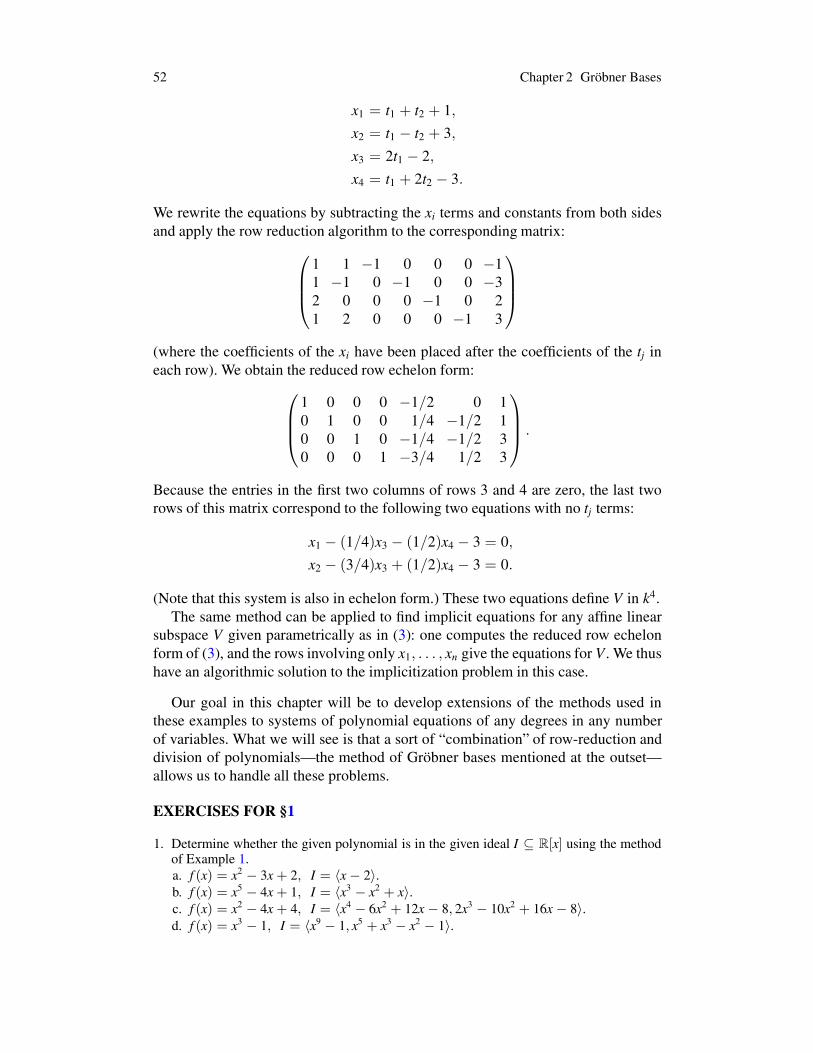
We rewrite the equations by subtracting the xi terms and constants from both sidesand apply the row reduction algorithm to the corresponding matrix:
⎛
⎜⎜⎝
1 1 −1 0 0 0 −11 −1 0 −1 0 0 −32 0 0 0 −1 0 21 2 0 0 0 −1 3
⎞
⎟⎟⎠
(where the coefficients of the xi have been placed after the coefficients of the tj ineach row). We obtain the reduced row echelon form:
⎛
⎜⎜⎝
1 0 0 0 −1/2 0 10 1 0 0 1/4 −1/2 10 0 1 0 −1/4 −1/2 30 0 0 1 −3/4 1/2 3
⎞
⎟⎟⎠ .
Because the entries in the first two columns of rows 3 and 4 are zero, the last tworows of this matrix correspond to the following two equations with no tj terms:
x1 − (1/4)x3 − (1/2)x4 − 3 = 0,
x2 − (3/4)x3 + (1/2)x4 − 3 = 0.
(Note that this system is also in echelon form.) These two equations define V in k4.The same method can be applied to find implicit equations for any affine linear
subspace V given parametrically as in (3): one computes the reduced row echelonform of (3), and the rows involving only x1, . . . , xn give the equations for V . We thushave an algorithmic solution to the implicitization problem in this case.
Our goal in this chapter will be to develop extensions of the methods used inthese examples to systems of polynomial equations of any degrees in any numberof variables. What we will see is that a sort of “combination” of row-reduction anddivision of polynomials—the method of Gröbner bases mentioned at the outset—allows us to handle all these problems.
EXERCISES FOR §1
1. Determine whether the given polynomial is in the given ideal I ⊆ R[x] using the methodof Example 1.a. f (x) = x2 − 3x+ 2, I = ⟨x− 2⟩.b. f (x) = x5 − 4x+ 1, I = ⟨x3 − x2 + x⟩.c. f (x) = x2 − 4x+ 4, I = ⟨x4 − 6x2 + 12x− 8, 2x3 − 10x2 + 16x− 8⟩.d. f (x) = x3 − 1, I = ⟨x9 − 1, x5 + x3 − x2 − 1⟩.

§1 Introduction 53
2. Find parametrizations of the affine varieties defined by the following sets of equations.a. In R3 or C3:
2x+ 3y− z = 9,x− y = 1,
3x+ 7y− 2z = 17.
b. In R4 or C4:
x1 + x2 − x3 − x4 = 0,x1 − x2 + x3 = 0.
c. In R3 or C3:
y− x3 = 0,
z− x5 = 0.
3. Find implicit equations for the affine varieties parametrized as follows.a. In R3 or C3:
x1 = t − 5,x2 = 2t + 1,x3 = −t + 6.
b. In R4 or C4:
x1 = 2t − 5u,x2 = t + 2u,x3 = −t + u,x4 = t + 3u.
c. In R3 or C3:x = t, y = t4, z = t7.
4. Let x1, x2, x3, . . . be an infinite collection of independent variables indexed by the naturalnumbers. A polynomial with coefficients in a field k in the xi is a finite linear combinationof (finite) monomials xe1i1 . . . x
enin . Let R denote the set of all polynomials in the xi. Note that
we can add and multiply elements of R in the usual way. Thus, R is the polynomial ringk[x1, x2, . . .] in infinitely many variables.a. Let I = ⟨x1, x2, x3, . . .⟩ be the set of polynomials of the form xt1 f1+ · · ·+xtm fm, where
fj ∈ R. Show that I is an ideal in the ring R.b. Show, arguing by contradiction, that I has no finite generating set. Hint: It is not enough
only to consider subsets of {xi | i ≥ 1}.5. In this problem you will show that all polynomial parametric curves in k2 are contained in
affine algebraic varieties.a. Show that the number of distinct monomials xayb of total degree≤ m in k[x, y] is equal
to (m+ 1)(m+ 2)/2. [Note: This is the binomial coefficient(m+2
2
).]
b. Show that if f (t) and g(t) are polynomials of degree ≤ n in t, then for m large enough,the “monomials”
[ f (t)]a[g(t)]b
with a+ b ≤ m are linearly dependent.

54 Chapter 2 Gröbner Bases
c. Deduce from part (b) that if C is a curve in k2 given parametrically by x = f (t), y =g(t) for f (t), g(t) ∈ k[t], then C is contained in V(F) for some nonzero F ∈ k[x, y].
d. Generalize parts (a), (b), and (c) to show that any polynomial parametric surface
x = f (t, u), y = g(t, u), z = h(t, u)
is contained in an algebraic surface V(F), where F ∈ k[x, y, z] is nonzero.
§2 Orderings on the Monomials in k[x1, . . . , xn]
If we examine the division algorithm in k[x] and the row-reduction (Gaussian elimi-nation) algorithm for systems of linear equations (or matrices) in detail, we see that anotion of ordering of terms in polynomials is a key ingredient of both (though this isnot often stressed). For example, in dividing f (x) = x5−3x2+1 by g(x) = x2−4x+7by the standard method, we would:• Write the terms in the polynomials in decreasing order by degree in x.• At the first step, the leading term (the term of highest degree) in f is x5 = x3 · x2 =
x3 · (leading term in g). Thus, we would subtract x3 · g(x) from f to cancel theleading term, leaving 4x4 − 7x3 − 3x2 + 1.
• Then, we would repeat the same process on f (x)− x3 · g(x), etc., until we obtaina polynomial of degree less than 2.
For the division algorithm on polynomials in one variable, we are dealing with thedegree ordering on the one-variable monomials:
(1) · · · > xm+1 > xm > · · · > x2 > x > 1.
The success of the algorithm depends on working systematically with the leadingterms in f and g, and not removing terms “at random” from f using arbitrary termsfrom g.
Similarly, in the row-reduction algorithm on matrices, in any given row, we sys-tematically work with entries to the left first—leading entries are those nonzero en-tries farthest to the left on the row. On the level of linear equations, this is expressedby ordering the variables x1, . . . , xn as follows:
(2) x1 > x2 > · · · > xn.
We write the terms in our equations in decreasing order. Furthermore, in an echelonform system, the equations are listed with their leading terms in decreasing order.(In fact, the precise definition of an echelon form system could be given in terms ofthis ordering—see Exercise 8.)
From the above evidence, we might guess that a major component of any exten-sion of division and row-reduction to arbitrary polynomials in several variables willbe an ordering on the terms in polynomials in k[x1, . . . , xn]. In this section, we willdiscuss the desirable properties such an ordering should have, and we will construct

§2 Orderings on the Monomials in k[x1, . . . , xn] 55
several different examples that satisfy our requirements. Each of these orderingswill be useful in different contexts.
First, we note that we can reconstruct the monomial xα = xα11 · · · xαn
n fromthe n-tuple of exponents α = (α1, . . . ,αn) ∈ Zn
≥0. This observation establishes aone-to-one correspondence between the monomials in k[x1, . . . , xn] and Zn
≥0. Fur-thermore, any ordering> we establish on the space Zn
≥0 will give us an ordering onmonomials: if α > β according to this ordering, we will also say that xα > xβ .
There are many different ways to define orderings on Zn≥0. For our purposes,
most of these orderingswill not be useful, however, since we will want our orderingsto be compatible with the algebraic structure of polynomial rings.
To begin, since a polynomial is a sum of monomials, we would like to be ableto arrange the terms in a polynomial unambiguously in descending (or ascending)order. To do this, we must be able to compare every pair of monomials to establishtheir proper relative positions. Thus, we will require that our orderings be linear ortotal orderings. This means that for every pair of monomials xα and x β , exactly oneof the three statements
xα > x β, xα = x β , x β > xα
should be true. A total order is also required to be transitive, so that xα > x β andx β > xγ always imply xα > xγ .
Next, we must take into account the effect of the sum and product operationson polynomials. When we add polynomials, after combining like terms, we maysimply rearrange the terms present into the appropriate order, so sums present nodifficulties. Products are more subtle, however. Since multiplication in a polynomialring distributes over addition, it suffices to consider what happens when we multiplya monomial times a polynomial. If doing this changed the relative ordering of terms,significant problems could result in any process similar to the division algorithm ink[x], in which we must identify the leading terms in polynomials. The reason is thatthe leading term in the product could be different from the product of the monomialand the leading term of the original polynomial.
Hence, we will require that all monomial orderings have the following additionalproperty. If xα > xβ and xγ is any monomial, then we require that xαxγ > xβxγ . Interms of the exponent vectors, this property means that if α > β in our ordering onZn≥0, then, for all γ ∈ Zn
≥0,α+ γ > β + γ.With these considerations in mind, we make the following definition.
Definition 1. A monomial ordering > on k[x1, . . . , xn] is a relation > on Zn≥0, or
equivalently, a relation on the set of monomials xα,α ∈ Zn≥0, satisfying:
(i) > is a total (or linear) ordering on Zn≥0.
(ii) If α > β and γ ∈ Zn≥0, then α+ γ > β + γ.
(iii) > is a well-ordering on Zn≥0. This means that every nonempty subset of Zn
≥0has a smallest element under >. In other words, if A ⊆ Zn
≥0 is nonempty, thenthere is α ∈ A such that β > α for every β = α in A.
Given a monomial ordering>, we say that α ≥ β when either α > β or α = β.

56 Chapter 2 Gröbner Bases
The following lemma will help us understand what the well-ordering conditionof part (iii) of the definition means.
Lemma 2. An order relation> on Zn≥0 is a well-ordering if and only if every strictly
decreasing sequence in Zn≥0
α(1) > α(2) > α(3) > · · ·
eventually terminates.
Proof. We will prove this in contrapositive form: > is not a well-ordering if andonly if there is an infinite strictly decreasing sequence in Zn
≥0.If > is not a well-ordering, then some nonempty subset S ⊆ Zn
≥0 has no leastelement. Now pick α(1) ∈ S. Since α(1) is not the least element, we can findα(1) > α(2) in S. Then α(2) is also not the least element, so that there is α(2) >α(3) in S. Continuing this way, we get an infinite strictly decreasing sequence
α(1) > α(2) > α(3) > · · · .
Conversely, given such an infinite sequence, then {α(1),α(2),α(3), . . .} is a non-empty subset of Zn
≥0 with no least element, and thus, > is not a well-ordering. !The importance of this lemma will become evident in what follows. It will be
used to show that various algorithms must terminate because some term strictlydecreases (with respect to a fixed monomial order) at each step of the algorithm.
In §4, we will see that given parts (i) and (ii) in Definition 1, the well-orderingcondition of part (iii) is equivalent to α ≥ 0 for all α ∈ Zn
≥0.For a simple example of a monomial order, note that the usual numerical order
· · · > m+ 1 > m > · · · > 3 > 2 > 1 > 0
on the elements of Z≥0 satisfies the three conditions of Definition 1. Hence, thedegree ordering (1) on the monomials in k[x] is a monomial ordering, unique byExercise 13.
Our first example of an ordering on n-tuples will be lexicographic order (or lexorder, for short).
Definition 3 (Lexicographic Order). Let α = (α1, . . . ,αn) and β = (β1, . . . ,βn)be in Zn
≥0. We say α >lex β if the leftmost nonzero entry of the vector differenceα− β ∈ Zn is positive. We will write xα >lex xβ if α >lex β.
Here are some examples:a. (1, 2, 0) >lex (0, 3, 4) since α− β = (1,−1,−4).b. (3, 2, 4) >lex (3, 2, 1) since α− β = (0, 0, 3).c. The variables x1, . . . , xn are ordered in the usual way [see (2)] by the lex ordering:
(1, 0, . . . , 0) >lex (0, 1, 0, . . . , 0) >lex · · · >lex (0, . . . , 0, 1).
so x1 >lex x2 >lex · · · >lex xn.
§2 Orderings on the Monomials in k[x1, . . . , xn] 57
In practice, when we work with polynomials in two or three variables, we willcall the variables x, y, z rather than x1, x2, x3. We will also assume that the alphabet-ical order x > y > z on the variables is used to define the lexicographic orderingunless we explicitly say otherwise.
Lex order is analogous to the ordering of words used in dictionaries (hence thename). We can view the entries of an n-tuple α ∈ Zn
≥0 as analogues of the letters ina word. The letters are ordered alphabetically:
a > b > · · · > y > z.
Then, for instance,arrow >lex arson
since the third letter of “arson” comes after the third letter of “arrow” in alphabeticalorder, whereas the first two letters are the same in both. Since all elements α ∈ Zn
≥0have length n, this analogy only applies to words with a fixed number of letters.
For completeness, we must check that the lexicographic order satisfies the threeconditions of Definition 1.
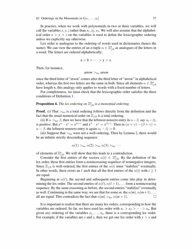
Proposition 4. The lex ordering on Zn≥0 is a monomial ordering.
Proof. (i) That >lex is a total ordering follows directly from the definition and thefact that the usual numerical order on Z≥0 is a total ordering.
(ii) If α >lex β, then we have that the leftmost nonzero entry in α−β, say αi−βi,is positive. But xα · xγ = xα+γ and xβ · xγ = xβ+γ . Then in (α+ γ)− (β + γ) =α− β, the leftmost nonzero entry is again αi − βi > 0.
(iii) Suppose that >lex were not a well-ordering. Then by Lemma 2, there wouldbe an infinite strictly descending sequence
α(1) >lex α(2) >lex α(3) >lex · · ·
of elements of Zn≥0. We will show that this leads to a contradiction.
Consider the first entries of the vectors α(i) ∈ Zn≥0. By the definition of the
lex order, these first entries form a nonincreasing sequence of nonnegative integers.Since Z≥0 is well-ordered, the first entries of the α(i) must “stabilize” eventually.In other words, there exists an ℓ such that all the first entries of the α(i) with i ≥ ℓare equal.
Beginning at α(ℓ), the second and subsequent entries come into play in deter-mining the lex order. The second entries of α(ℓ),α(ℓ+ 1), . . . form a nonincreasingsequence. By the same reasoning as before, the second entries “stabilize” eventuallyas well. Continuing in the same way, we see that for somem, the α(m),α(m+1), . . .all are equal. This contradicts the fact that α(m) >lex α(m+ 1). !
It is important to realize that there are many lex orders, corresponding to how thevariables are ordered. So far, we have used lex order with x1 > x2 > · · · > xn. Butgiven any ordering of the variables x1, . . . , xn, there is a corresponding lex order.For example, if the variables are x and y, then we get one lex order with x > y and

58 Chapter 2 Gröbner Bases
a second with y > x. In the general case of n variables, there are n! lex orders. Inwhat follows, the phrase “lex order” will refer to the one with x1 > · · · > xn unlessotherwise stated.
In lex order, notice that a variable dominates any monomial involving onlysmaller variables, regardless of its total degree. Thus, for the lex order with x >y > z, we have x >lex y5z3. For some purposes, we may also want to take the totaldegrees of the monomials into account and order monomials of bigger degree first.One way to do this is the graded lexicographic order (or grlex order).
Definition 5 (Graded Lex Order). Let α,β ∈ Zn≥0. We say α >grlex β if
|α| =n∑
i=1
αi > |β| =n∑
i=1
βi, or |α| = |β| and α >lex β.
We see that grlex orders by total degree first, then “break ties” using lex order.Here are some examples:a. (1, 2, 3) >grlex (3, 2, 0) since |(1, 2, 3)| = 6 > |(3, 2, 0)| = 5.b. (1, 2, 4) >grlex (1, 1, 5) since |(1, 2, 4)| = |(1, 1, 5)| and (1, 2, 4) >lex (1, 1, 5).c. The variables are ordered according to the lex order, i.e., x1 >grlex · · · >grlex xn.
We will leave it as an exercise to show that the grlex ordering satisfies the threeconditions of Definition 1. As in the case of lex order, there are n! grlex orderson n variables, depending on how the variables are ordered.Another (somewhat less intuitive) order on monomials is the graded reverse lexi-
cographical order (or grevlex order). Even though this ordering “takes some gettingused to,” it has been shown that for some operations, the grevlex ordering is the mostefficient for computations.
Definition 6 (Graded Reverse Lex Order). Let α,β ∈ Zn≥0. We say α >grevlex β if
|α| =n∑
i=1
αi > |β| =n∑
i=1
βi, or |α| = |β| and the rightmost nonzero entryof α− β ∈ Zn is negative.
Like grlex, grevlex orders by total degree, but it “breaks ties” in a different way.For example:a. (4, 7, 1) >grevlex (4, 2, 3) since |(4, 7, 1)| = 12 > |(4, 2, 3)| = 9.b. (1, 5, 2) >grevlex (4, 1, 3) since |(1, 5, 2)| = |(4, 1, 3)| and (1, 5, 2) −(4, 1, 3) =
(−3, 4,−1).You will show in the exercises that the grevlex ordering gives a monomial ordering.
Note also that lex and grevlex give the same ordering on the variables. That is,
(1, 0, . . . , 0) >grevlex (0, 1, . . . , 0) >grevlex · · · >grevlex (0, . . . , 0, 1)
orx1 >grevlex x2 >grevlex · · · >grevlex xn

§2 Orderings on the Monomials in k[x1, . . . , xn] 59
Thus, grevlex is really different from the grlex order with the variables rearranged(as one might be tempted to believe from the name).
To explain the relation between grlex and grevlex, note that both use total degreein the same way. To break a tie, grlex uses lex order, so that it looks at the leftmost(or largest) variable and favors the larger power. In contrast, when grevlex findsthe same total degree, it looks at the rightmost (or smallest) variable and favorsthe smaller power. In the exercises, you will check that this amounts to a “double-reversal” of lex order. For example,
x5yz >grlex x4yz2,
since both monomials have total degree 7 and x5yz >lex x4yz2. In this case, we alsohave
x5yz >grevlex x4yz2,
but for a different reason: x5yz is larger because the smaller variable z appears to asmaller power.
As with lex and grlex, there are n! grevlex orderings corresponding to how the nvariables are ordered.
There are many other monomial orders besides the ones considered here. Someof these will be explored in the exercises for §4. Most computer algebra systemsimplement lex order, and most also allow other orders, such as grlex and grevlex.Once such an order is chosen, these systems allow the user to specify any of the n!orderings of the variables. As we will see in §8 of this chapter and in later chapters,this facility becomes very useful when studying a variety of questions.
We will end this section with a discussion of how a monomial ordering can beapplied to polynomials. If f =
∑α aαxα is a nonzero polynomial in k[x1, . . . , xn]
and we have selected a monomial ordering >, then we can order the monomials off in an unambiguous way with respect to >. For example, consider the polynomialf = 4xy2z+ 4z2 − 5x3 + 7x2z2 ∈ k[x, y, z]. Then:• With respect to lex order, we would reorder the terms of f in decreasing order as
f = −5x3 + 7x2z2 + 4xy2z+ 4z2.
• With respect to grlex order, we would have
f = 7x2z2 + 4xy2z− 5x3 + 4z2.
• With respect to grevlex order, we would have
f = 4xy2z+ 7x2z2 − 5x3 + 4z2.
We will use the following terminology.
Definition 7. Let f =∑
α aαxα be a nonzero polynomial in k[x1, . . . , xn] and let >be a monomial order.

60 Chapter 2 Gröbner Bases
(i) Themultidegree of f is
multideg( f ) = max(α ∈ Zn≥0 | aα = 0)
(the maximum is taken with respect to >).(ii) The leading coefficient of f is
LC( f ) = amultideg( f ) ∈ k.
(iii) The leading monomial of f is
LM( f ) = xmultideg( f )
(with coefficient 1).(iv) The leading term of f is
LT( f ) = LC( f ) · LM( f ).
To illustrate, let f = 4xy2z + 4z2 − 5x3 + 7x2z2 as before and let > denote lexorder. Then
multideg( f ) = (3, 0, 0),
LC( f ) = −5,
LM( f ) = x3,
LT( f ) = −5x3.
In the exercises, you will show that the multidegree has the following usefulproperties.
Lemma 8. Let f , g ∈ k[x1, . . . , xn] be nonzero polynomials. Then:(i) multideg( fg) = multideg( f ) +multideg(g).(ii) If f + g = 0, then multideg( f + g) ≤ max(multideg( f ),multideg(g)). If, in
addition,multideg( f ) = multideg(g), then equality occurs.
Some books use different terminology. In EISENBUD (1999), the leading termLT( f ) becomes the initial term in>( f ). A more substantial difference appears inBECKER and WEISPFENNING (1993), where the meanings of “monomial” and“term” are interchanged. For them, the leading term LT( f ) is the head monomialHM( f ), while the leading monomial LM( f ) is the head term HT( f ). Page 10 ofKREUZER and ROBBIANO (2000) has a summary of the terminology used in differ-ent books. Our advice when reading other texts is to check the definitions carefully.
EXERCISES FOR §2
1. Rewrite each of the following polynomials, ordering the terms using the lex order, thegrlex order, and the grevlex order, giving LM( f ), LT( f ), and multideg( f ) in each case.

§3 A Division Algorithm in k[x1, . . . , xn] 61
a. f (x, y, z) = 2x+ 3y+ z+ x2 − z2 + x3.b. f (x, y, z) = 2x2y8 − 3x5yz4 + xyz3 − xy4.
2. Each of the following polynomials is written with its monomials ordered according to(exactly) one of lex, grlex, or grevlex order. Determine which monomial order was usedin each case.a. f (x, y, z) = 7x2y4z− 2xy6 + x2y2.b. f (x, y, z) = xy3z + xy2z2 + x2z3.c. f (x, y, z) = x4y5z+ 2x3y2z− 4xy2z4.
3. Repeat Exercise 1 when the variables are ordered z > y > x.4. Show that grlex is a monomial order according to Definition 1.5. Show that grevlex is a monomial order according to Definition 1.6. Another monomial order is the inverse lexicographic or invlex order defined by the
following: for α,β ∈ Zn≥0,α >invlex β if and only if the rightmost nonzero entry of
α − β is positive. Show that invlex is equivalent to the lex order with the variablespermuted in a certain way. (Which permutation?)
7. Let > be any monomial order.a. Show that α ≥ 0 for all α ∈ Zn
≥0. Hint: Proof by contradiction.b. Show that if xα divides xβ , then α ≤ β. Is the converse true?c. Show that if α ∈ Zn
≥0, then α is the smallest element of α + Zn≥0 = {α + β | β ∈
Zn≥0}.
8. Write a precise definition of what it means for a system of linear equations to be inechelon form, using the ordering given in equation (2).
9. In this exercise, we will study grevlex in more detail. Let >invlex, be the order given inExercise 6, and define >rinvlex to be the reversal of this ordering, i.e., for α, β ∈ Zn
≥0.
α >rinvlex β ⇐⇒ β >invlex α.
Notice that rinvlex is a “double reversal” of lex, in the sense that we first reverse theorder of the variables and then we reverse the ordering itself.a. Show that α >grevlex β if and only if |α| > |β|, or |α| = |β| and α >rinvlex β.b. Is rinvlex a monomial ordering according to Definition 1? If so, prove it; if not, say
which properties fail.10. In Z≥0 with the usual ordering, between any two integers, there are only a finite number
of other integers. Is this necessarily true in Zn≥0 for a monomial order? Is it true for the
grlex order?11. Let > be a monomial order on k[x1, . . . , xn].
a. Let f ∈ k[x1, . . . , xn] and let m be a monomial. Show that LT(m · f ) = m · LT( f ).b. Let f , g ∈ k[x1, . . . , xn]. Is LT( f · g) necessarily the same as LT( f ) · LT(g)?c. If fi, gi ∈ k[x1, . . . , xn], 1 ≤ i ≤ s, is LM(
∑si=1 figi) necessarily equal to LM( fi) ·
LM(gi) for some i?12. Lemma 8 gives two properties of the multidegree.
a. Prove Lemma 8. Hint: The arguments used in Exercise 11 may be relevant.b. Suppose that multideg( f ) = multideg(g) and f + g = 0. Give examples to show that
multideg( f + g) may or may not equal max(multideg( f ), multideg(g)).13. Prove that 1 < x < x2 < x3 < · · · is the unique monomial order on k[x].
§3 A Division Algorithm in k[x1, . . . , xn]
In §1, we saw how the division algorithm could be used to solve the ideal mem-bership problem for polynomials of one variable. To study this problem whenthere are more variables, we will formulate a division algorithm for polynomials

62 Chapter 2 Gröbner Bases
in k[x1, . . . , xn] that extends the algorithm for k[x]. In the general case, the goal isto divide f ∈ k[x1, . . . , xn] by f1, . . . , fs ∈ k[x1, . . . , xn]. As we will see, this meansexpressing f in the form
f = q1 f1 + · · ·+ qs fs + r,
where the “quotients” q1, . . . , qs and remainder r lie in k[x1, . . . , xn]. Some care willbe needed in deciding how to characterize the remainder. This is where we willuse the monomial orderings introduced in §2. We will then see how the divisionalgorithm applies to the ideal membership problem.
The basic idea of the algorithm is the same as in the one-variable case: we want tocancel the leading term of f (with respect to a fixed monomial order) by multiplyingsome fi by an appropriate monomial and subtracting. Then this monomial becomesa term in the corresponding qi. Rather than state the algorithm in general, let us firstwork through some examples to see what is involved.
Example 1. We will first divide f = xy2 + 1 by f1 = xy + 1 and f2 = y + 1, usinglex order with x > y. We want to employ the same scheme as for division of one-variable polynomials, the difference being that there are now several divisors andquotients. Listing the divisors f1, f2 and the quotients q1, q2 vertically, we have thefollowing setup:
q1 :q2 :
xy+ 1y+ 1
)xy2 + 1
The leading terms LT( f1) = xy and LT( f2) = y both divide the leading term LT( f ) =xy2. Since f1 is listed first, we will use it. Thus, we divide xy into xy2, leaving y, andthen subtract y · f1 from f :
q1 : yq2 :
xy+ 1y+ 1
)xy2 + 1xy2 + y
−y+ 1
Now we repeat the same process on−y+1. This time we must use f2 since LT( f1) =xy does not divide LT(−y+ 1) = −y. We obtain:
q1 : yq2 : −1
xy+ 1y+ 1
)xy2 + 1xy2 + y
−y+ 1−y− 1
2

§3 A Division Algorithm in k[x1, . . . , xn] 63
Since LT( f1) and LT( f2) do not divide 2, the remainder is r = 2 and we are done.Thus, we have written f = xy2 + 1 in the form
xy2 + 1 = y · (xy+ 1) + (−1) · (y+ 1) + 2.
Example 2. In this example, we will encounter an unexpected subtlety that canoccur when dealing with polynomials of more than one variable. Let us dividef = x2y + xy2 + y2 by f1 = xy − 1 and f2 = y2 − 1. As in the previous exam-ple, we will use lex order with x > y. The first two steps of the algorithm go asusual, giving us the following partially completed division (remember that whenboth leading terms divide, we use f1):
q1 : x+ yq2 :
xy− 1y2 − 1
)x2y+ xy2 + y2
x2y− x
xy2 + x+ y2
xy2 − y
x+ y2 + y
Note that neither LT( f1) = xy nor LT( f2) = y2 divides LT(x+ y2+ y) = x. However,x + y2 + y is not the remainder since LT( f2) divides y2. Thus, if we move x to theremainder, we can continue dividing. (This is something that never happens in theone-variable case: once the leading term of the divisor no longer divides the leadingterm of what is at the bottom of the division, the algorithm terminates.)
To implement this idea, we create a remainder column r, to the right of the divi-sion, where we put the terms belonging to the remainder. Also, we call the polyno-mial at the bottom of division the intermediate dividend. Then we continue dividinguntil the intermediate dividend is zero. Here is the next step, where we move x tothe remainder column (as indicated by the arrow):
q1 : x+ yq2 :
xy− 1y2 − 1
)x2y+ xy2 + y2
xy2 − x
xy2 + x+ y2
x2y− y
x+ y2 + yy2 + y
r
−→ x
Now we continue dividing. If we can divide by LT( f1) or LT( f2), we proceed asusual, and if neither divides, we move the leading term of the intermediate dividendto the remainder column.

64 Chapter 2 Gröbner Bases
Here is the rest of the division:
q1 : x+ yq2 : 1
xy− 1y2 − 1
)x2y+ xy2 + y2
x2y− x
xy2 + x+ y2
xy2 − y
x+ y2 + yy2 + y
r
−→ xy2 − 1
y+ 11 −→ x+ y0 −→ x+ y+ 1
Thus, the remainder is x+ y+ 1, and we obtain
(1) x2y+ xy2 + y2 = (x+ y) · (xy− 1) + 1 · (y2 − 1) + x+ y+ 1.
Note that the remainder is a sum of monomials, none of which is divisible by theleading terms LT( f1) or LT( f2).
The above example is a fairly complete illustration of how the division algorithmworks. It also shows us what property we want the remainder to have: none of itsterms should be divisible by the leading terms of the polynomials by which we aredividing. We can now state the general form of the division algorithm.
Theorem 3 (Division Algorithm in k[x1, . . . , xn]). Let > be a monomial order onZn≥0, and let F = ( f1, . . . , fs) be an ordered s-tuple of polynomials in k[x1, . . . , xn].
Then every f ∈ k[x1, . . . , xn] can be written as
f = q1 f1 + · · ·+ qs fs + r,
where qi, r ∈ k[x1, . . . , xn], and either r = 0 or r is a linear combination, with coef-ficients in k, of monomials, none of which is divisible by any of LT( f1), . . . , LT( fs).We call r a remainder of f on division by F. Furthermore, if qi fi = 0, then
multideg( f ) ≥ multideg(qi fi).
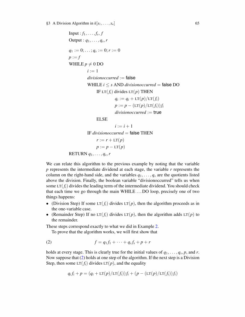
Proof. We prove the existence of q1, . . . , qs and r by giving an algorithm for theirconstruction and showing that it operates correctly on any given input. We recom-mend that the reader review the division algorithm in k[x] given in Proposition 2 ofChapter 1, §5 before studying the following generalization:
§3 A Division Algorithm in k[x1, . . . , xn] 65
Input : f1, . . . , fs, f
Output : q1, . . . , qs, r
q1 := 0; . . . ; qs := 0; r := 0
p := f
WHILE p = 0 DO
i := 1
divisionoccurred := falseWHILE i ≤ s AND divisionoccurred = false DO
IF LT( fi) divides LT(p) THEN
qi := qi + LT(p)/LT( fi)
p := p− (LT(p)/LT( fi)) fidivisionoccurred := true
ELSE
i := i+ 1
IF divisionoccurred = false THEN
r := r + LT(p)
p := p− LT(p)
RETURN q1, . . . , qs, r
We can relate this algorithm to the previous example by noting that the variablep represents the intermediate dividend at each stage, the variable r represents thecolumn on the right-hand side, and the variables q1, . . . , qs are the quotients listedabove the division. Finally, the boolean variable “divisionoccurred” tells us whensome LT( fi) divides the leading term of the intermediate dividend. You should checkthat each time we go through the main WHILE . . .DO loop, precisely one of twothings happens:• (Division Step) If some LT( fi) divides LT(p), then the algorithm proceeds as in
the one-variable case.• (Remainder Step) If no LT( fi) divides LT(p), then the algorithm adds LT(p) to
the remainder.These steps correspond exactly to what we did in Example 2.
To prove that the algorithm works, we will first show that
(2) f = q1 f1 + · · ·+ qs fs + p+ r
holds at every stage. This is clearly true for the initial values of q1, . . . , qs, p, and r.Now suppose that (2) holds at one step of the algorithm. If the next step is a DivisionStep, then some LT( fi) divides LT(p), and the equality
qi fi + p = (qi + LT(p)/LT( fi)) fi + (p− (LT(p)/LT( fi)) fi)

66 Chapter 2 Gröbner Bases
shows that qi fi+p is unchanged. Since all other variables are unaffected, (2) remainstrue in this case. On the other hand, if the next step is a Remainder Step, then p andr will be changed, but the sum p+ r is unchanged since
p+ r = (p− LT(p)) + (r + LT(p)).
As before, equality (2) is still preserved.Next, notice that the algorithm comes to a halt when p = 0. In this situation, (2)
becomesf = q1 f1 + · · ·+ qs fs + r.
Since terms are added to r only when they are divisible by none of the LT( fi), it fol-lows that q1, . . . , qs and r have the desired properties when the algorithm terminates.
Finally, we need to show that the algorithm does eventually terminate. The keyobservation is that each time we redefine the variable p, either its multidegree drops(relative to our term ordering) or it becomes 0. To see this, first suppose that duringa Division Step, p is redefined to be
p′ = p− LT(p)LT( fi)
fi.
By Lemma 8 of §2, we have
LT( LT(p)LT( fi)
fi)=
LT(p)LT( fi)
LT( fi) = LT(p),
so that p and (LT(p)/LT( fi)) fi have the same leading term. Hence, their differencep′ must have strictly smaller multidegree when p′ = 0. Next, suppose that during aRemainder Step, p is redefined to be
p′ = p− LT(p).
Here, it is obvious that multideg(p′) < multideg(p) when p′ = 0. Thus, in ei-ther case, the multidegree must decrease. If the algorithm never terminated, then wewould get an infinite decreasing sequence of multidegrees. The well-ordering prop-erty of >, as stated in Lemma 2 of §2, shows that this cannot occur. Thus p = 0must happen eventually, so that the algorithm terminates after finitely many steps.
It remains to study the relation between multideg( f ) and multideg(qi fi). Everyterm in qi is of the form LT(p)/LT( fi) for some value of the variable p. The algorithmstarts with p = f , and we just finished proving that the multidegree of p decreases.This shows that LT(p) ≤ LT( f ), and then it follows easily [using condition (ii) of thedefinition of a monomial order] that multideg(qi fi) ≤ multideg( f ) when qi fi = 0(see Exercise 4). This completes the proof of the theorem. !
The algebra behind the division algorithm is very simple (there is nothing beyondhigh school algebra in what we did), which makes it surprising that this form of thealgorithm was first isolated and exploited only within the past 50 years.
§3 A Division Algorithm in k[x1, . . . , xn] 67
We will conclude this section by asking whether the division algorithm has thesame nice properties as the one-variable version. Unfortunately, the answer is notpretty—the examples given below will show that the division algorithm is far fromperfect. In fact, the algorithm achieves its full potential only when coupled with theGröbner bases studied in §§5 and 6.
A first important property of the division algorithm in k[x] is that the remainder isuniquely determined. To see how this can fail when there is more than one variable,consider the following example.
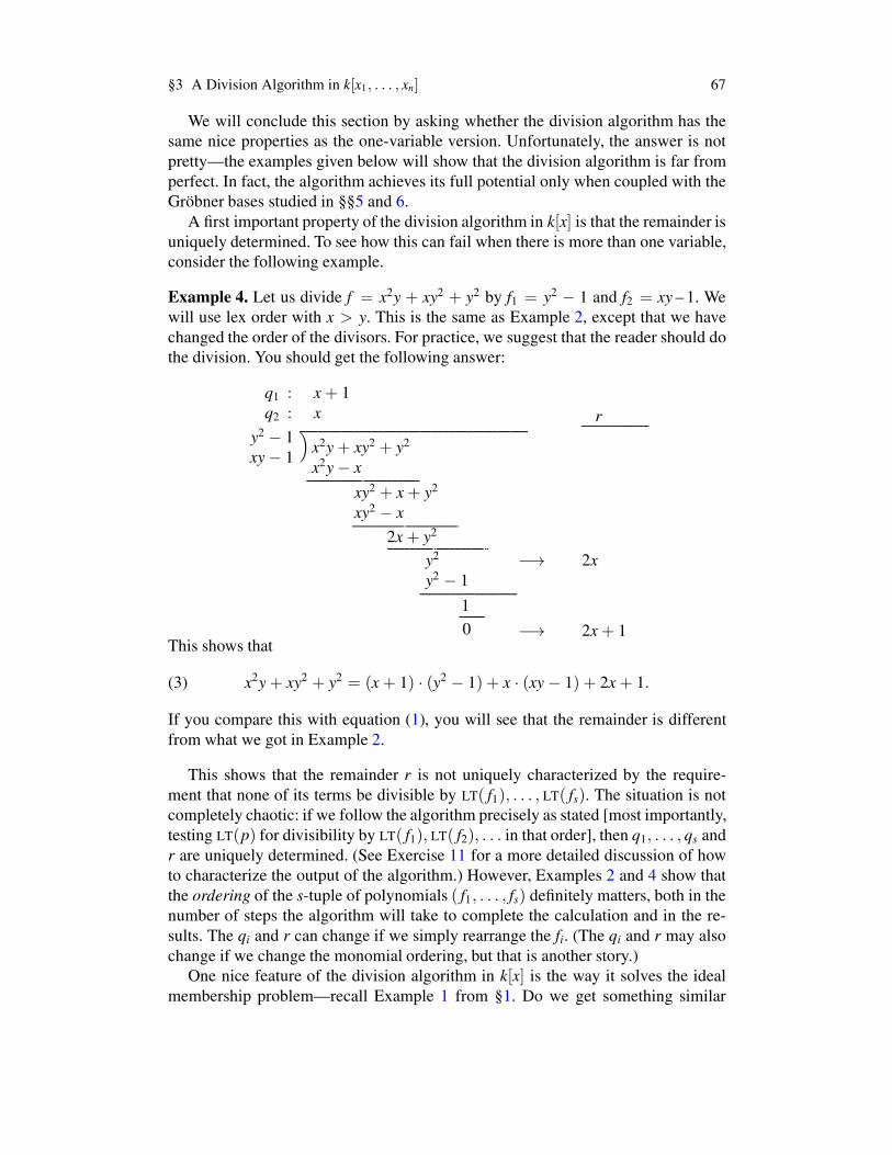
Example 4. Let us divide f = x2y + xy2 + y2 by f1 = y2 − 1 and f2 = xy – 1. Wewill use lex order with x > y. This is the same as Example 2, except that we havechanged the order of the divisors. For practice, we suggest that the reader should dothe division. You should get the following answer:
q1 : x+ 1q2 : x
y2 − 1xy− 1
)x2y+ xy2 + y2
x2y− x
xy2 + x+ y2
xy2 − x2x+ y2
y2
r
−→ 2xy2 − 1
10 −→ 2x+ 1
This shows that
(3) x2y+ xy2 + y2 = (x+ 1) · (y2 − 1) + x · (xy− 1) + 2x+ 1.
If you compare this with equation (1), you will see that the remainder is differentfrom what we got in Example 2.
This shows that the remainder r is not uniquely characterized by the require-ment that none of its terms be divisible by LT( f1), . . . , LT( fs). The situation is notcompletely chaotic: if we follow the algorithm precisely as stated [most importantly,testing LT(p) for divisibility by LT( f1), LT( f2), . . . in that order], then q1, . . . , qs andr are uniquely determined. (See Exercise 11 for a more detailed discussion of howto characterize the output of the algorithm.) However, Examples 2 and 4 show thatthe ordering of the s-tuple of polynomials ( f1, . . . , fs) definitely matters, both in thenumber of steps the algorithm will take to complete the calculation and in the re-sults. The qi and r can change if we simply rearrange the fi. (The qi and r may alsochange if we change the monomial ordering, but that is another story.)
One nice feature of the division algorithm in k[x] is the way it solves the idealmembership problem—recall Example 1 from §1. Do we get something similar

68 Chapter 2 Gröbner Bases
for several variables? One implication is an easy corollary of Theorem 3: if afterdivision of f by F = ( f1, . . . , fs) we obtain a remainder r = 0, then
f = q1 f1 + · · ·+ qs fs,
so that f ∈ ⟨ f1, . . . , fs⟩. Thus r = 0 is a sufficient condition for ideal membership.However, as the following example shows, r = 0 is not a necessary condition forbeing in the ideal.
Example 5. Let f1 = xy − 1, f2 = y2 − 1 ∈ k[x, y] with the lex order. Dividingf = xy2 − x by F = ( f1, f2), the result is
xy2 − x = y · (xy− 1) + 0 · (y2 − 1) + (−x+ y).
With F = ( f2, f1), however, we have
xy2 − x = x · (y2 − 1) + 0 · (xy− 1) + 0.
The second calculation shows that f ∈ ⟨ f1, f2⟩. Then the first calculation shows thateven if f ∈ ⟨ f1, f2⟩, it is still possible to obtain a nonzero remainder on division byF = ( f1, f2).
Thus, we must conclude that the division algorithm given in Theorem 3 is animperfect generalization of its one-variable counterpart. To remedy this situation,we turn to one of the lessons learned in Chapter 1. Namely, in dealing with a col-lection of polynomials f1, . . . , fs ∈ k[x1, . . . , xn], it is frequently desirable to passto the ideal I they generate. This allows the possibility of going from f1, . . . , fs to adifferent generating set for I. So we can still ask whether there might be a “good”generating set for I. For such a set, we would want the remainder r on division bythe “good” generators to be uniquely determined and the condition r = 0 should beequivalent to membership in the ideal. In §6, we will see that Gröbner bases haveexactly these “good” properties.
In the exercises, you will experiment with a computer algebra system to try todiscover for yourself what properties a “good” generating set should have. We willgive a precise definition of “good” in §5 of this chapter.
EXERCISES FOR §3
1. Compute the remainder on division of the given polynomial f by the ordered set F (byhand). Use the grlex order, then the lex order in each case.a. f = x7y2 + x3y2 − y+ 1, F = (xy2 − x, x− y3).b. Repeat part (a) with the order of the pair F reversed.
2. Compute the remainder on division:a. f = xy2z2 + xy− yz, F = (x− y2, y− z3, z2 − 1).b. Repeat part (a) with the order of the set F permuted cyclically.
3. Using a computer algebra system, check your work from Exercises 1 and 2. (You mayneed to consult documentation to learn whether the system you are using has an explicitpolynomial division command or you will need to perform the individual steps of thealgorithm yourself.)
§3 A Division Algorithm in k[x1, . . . , xn] 69
4. Let f = q1 f1 + · · ·+ qs fs + r be the output of the division algorithm.a. Complete the proof begun in the text that multideg( f ) ≥ multideg(qi fi) provided that
qi fi = 0.b. Prove that multideg( f ) ≥ multideg(r) when r = 0.
The following problems investigate in greater detail the way the remainder computed bythe division algorithm depends on the ordering and the form of the s-tuple of divisors F =( f1, . . . , fs). You may wish to use a computer algebra system to perform these calculations.
5. We will study the division of f = x3 − x2y− x2z+ x by f1 = x2y− z and f2 = xy− 1.a. Compute using grlex order:
r1 = remainder of f on division by ( f1, f2).r2 = remainder of f on division by ( f2, f1).
Your results should be different. Where in the division algorithm did the differenceoccur? (You may need to do a few steps by hand here.)
b. Is r = r1 − r2 in the ideal ⟨ f1, f2⟩? If so, find an explicit expression r = Af1 + Bf2. Ifnot, say why not.
c. Compute the remainder of r on division by ( f1, f2). Why could you have predictedyour answer before doing the division?
d. Find another polynomial g ∈ ⟨ f1, f2⟩ such that the remainder on division of g by( f1, f2) is nonzero. Hint: (xy+ 1) · f2 = x2y2 − 1, whereas y · f1 = x2y2 − yz.
e. Does the division algorithm give us a solution for the ideal membership problem forthe ideal ⟨ f1, f2⟩ ? Explain your answer.
6. Using the grlex order, find an element g of ⟨ f1, f2⟩ = ⟨2xy2 − x, 3x2y− y− 1⟩ ⊆ R[x, y]whose remainder on division by ( f1, f2) is nonzero. Hint: You can find such a g wherethe remainder is g itself.
7. Answer the question of Exercise 6 for ⟨ f1, f2, f3⟩ = ⟨x4y2 − z, x3y3 − 1, x2y4 − 2z⟩⊆ R[x, y, z]. Find two different polynomials g (not constant multiples of each other).
8. Try to formulate a general pattern that fits the examples in Exercises 5(c)(d), 6, and 7.What condition on the leading term of the polynomial g = A1 f1 + · · · + As fs wouldguarantee that there was a nonzero remainder on division by ( f1, . . . , fs)? What doesyour condition imply about the ideal membership problem?
9. The discussion around equation (2) of Chapter 1, §4 shows that every polynomial f ∈R[x, y, z] can be written as
f = h1(y− x2) + h2(z− x3) + r,
where r is a polynomial in x alone and V(y− x2, z− x3) is the twisted cubic curve in R3.a. Give a proof of this fact using the division algorithm. Hint: You need to specify
carefully the monomial ordering to be used.b. Use the parametrization of the twisted cubic to show that z2 − x4y vanishes at every
point of the twisted cubic.c. Find an explicit representation
z2 − x4y = h1(y− x2) + h2(z− x3)
using the division algorithm.10. Let V ⊆ R3 be the curve parametrized by (t, tm, tn), n,m ≥ 2.
a. Show that V is an affine variety.b. Adapt the ideas in Exercise 9 to determine I(V).

70 Chapter 2 Gröbner Bases
11. In this exercise, we will characterize completely the expression
f = q1 f1 + · · ·+ qs fs + r
that is produced by the division algorithm (among all the possible expressions for f ofthis form). Let LM( fi) = xα(i) and define
∆1 = α(1) + Zn≥0,
∆2 = (α(2) + Zn≥0) \∆1,
...
∆s = (α(s) + Zn≥0) \
( s−1⋃
i=1
∆i
),
∆ = Zn≥0 \
( s⋃
i=1
∆i
).
(Note that Zn≥0 is the disjoint union of the ∆i and ∆.)
a. Show that β ∈ ∆i if and only if xα(i) divides xβ and no xα(j) with j < i divides xβ .b. Show that γ ∈ ∆ if and only if no xα(i) divides xγ .c. Show that in the expression f = q1 f1 + · · · + qs fs + r computed by the division
algorithm, for every i, every monomial xβ in qi satisfies β + α(i) ∈ ∆i, and everymonomial xγ in r satisfies γ ∈ ∆.
d. Show that there is exactly one expression f = q1 f1 + · · · + qs fs + r satisfying theproperties given in part (c).
12. Show that the operation of computing remainders on division by F = ( f1, . . . , fs) islinear over k. That is, if the remainder on division of gi by F is ri, i = 1, 2, then, for anyc1, c2 ∈ k, the remainder on division of c1g1+c2g2 is c1r1+c2r2. Hint: Use Exercise 11.
§4 Monomial Ideals and Dickson’s Lemma
In this section, we will consider the ideal description problem of §1 for the specialcase of monomial ideals. This will require a careful study of the properties of theseideals. Our results will also have an unexpected application to monomial orderings.
To start, we define monomial ideals in k[x1, . . . , xn].
Definition 1. An ideal I ⊆ k[x1, . . . , xn] is a monomial ideal if there is a subsetA ⊆ Zn
≥0 (possibly infinite) such that I consists of all polynomials which are finitesums of the form
∑α∈A hαx
α, where hα ∈ k[x1, . . . , xn]. In this case, we writeI = ⟨xα | α ∈ A⟩.
An example of a monomial ideal is given by I = ⟨x4y2, x3y4, x2y5⟩ ⊆ k[x, y].More interesting examples of monomial ideals will be given in §5.
We first need to characterize all monomials that lie in a given monomial ideal.
Lemma 2. Let I = ⟨xα | α ∈ A⟩ be a monomial ideal. Then a monomial xβ lies in Iif and only if xβ is divisible by xα for some α ∈ A.

§4 Monomial Ideals and Dickson’s Lemma 71
Proof. If xβ is a multiple of xα for some α ∈ A, then xβ ∈ I by the definition ofideal. Conversely, if xβ ∈ I, then xβ =
∑si=1 hi x
α(i), where hi ∈ k[x1, . . . , xn] andα(i) ∈ A. If we expand each hi as a sum of terms, we obtain
xβ =s∑
i=1
hi xα(i) =s∑
i=1
(∑
j
ci, j xβ(i, j))xα(i) =
∑
i, j
ci, j xβ(i, j)xα(i).
After collecting terms of the same multidegree, every term on the right side of theequation is divisible by some xα(i). Hence, the left side xβ must have the sameproperty. !
Note that xβ is divisible by xα exactly when xβ = xα ·xγ for some γ ∈ Zn≥0. This
is equivalent to β = α+ γ. Thus, the set
α+ Zn≥0 = {α+ γ | γ ∈ Zn
≥0}
consists of the exponents of all monomials divisible by xα. This observation andLemma 2 allows us to draw pictures of the monomials in a given monomial ideal.For example, if I = ⟨x4y2, x3y4, x2y5⟩, then the exponents of the monomials in Iform the set
((4, 2) + Z2≥0) ∪ ((3, 4) + Z2
≥0) ∪ ((2, 5) + Z2≥0).
We can visualize this set as the union of the integer points in three translated copiesof the first quadrant in the plane:
n
m(m,n) ←→ xm yn
(2,5)
(3,4)
(4,2)
Let us next show that whether a given polynomial f lies in a monomial ideal canbe determined by looking at the monomials of f .
Lemma 3. Let I be a monomial ideal, and let f ∈ k[x1, . . . , xn]. Then the followingare equivalent:(i) f ∈ I.(ii) Every term of f lies in I.(iii) f is a k-linear combination of the monomials in I.

72 Chapter 2 Gröbner Bases
Proof. The implications (iii) ⇒ (ii) ⇒ (i) and (ii) ⇒ (iii) are trivial. The proof of(i)⇒ (ii) is similar to what we did in Lemma 2 and is left as an exercise. !
An immediate consequence of part (iii) of the lemma is that a monomial ideal isuniquely determined by its monomials. Hence, we have the following corollary.
Corollary 4. Two monomial ideals are the same if and only if they contain the samemonomials.
The main result of this section is that all monomial ideals of k[x1, . . . , xn] arefinitely generated.
Theorem 5 (Dickson’s Lemma). Let I = ⟨xα | α ∈ A⟩ ⊆ k[x1, . . . , xn] be amonomial ideal. Then I can be written in the form I = ⟨xα(1), . . . , xα(s)⟩, whereα(1), . . . ,α(s) ∈ A. In particular, I has a finite basis.
Proof. (By induction on n, the number of variables.) If n = 1, then I is generated bythe monomials xα1 , where α ∈ A ⊆ Z≥0. Let β be the smallest element of A ⊆ Z≥0.Then β ≤ α for all α ∈ A, so that xβ1 divides all other generators xα1 . From here,I = ⟨xβ1 ⟩ follows easily.
Now assume that n > 1 and that the theorem is true for n − 1. We will write thevariables as x1, . . . , xn−1, y, so that monomials in k[x1, . . . , xn−1, y] can be written asxαym, where α = (α1, . . . ,αn−1) ∈ Zn−1
≥0 and m ∈ Z≥0.Suppose that I ⊆ k[x1, . . . , xn−1, y] is a monomial ideal. To find generators for
I, let J be the ideal in k[x1, . . . , xn−1] generated by the monomials xα for whichxαym ∈ I for some m ≥ 0. Since J is a monomial ideal in k[x1, . . . , xn−1],our inductive hypothesis implies that finitely many of the xα’s generate J, sayJ = ⟨xα(1), . . . , xα(s)⟩. The ideal J can be understood as the “projection” of I intok[x1, . . . , xn−1].
For each i between 1 and s, the definition of J tells us that xα(i)ymi ∈ I for somemi ≥ 0. Let m be the largest of the mi. Then, for each ℓ between 0 and m − 1,consider the ideal Jℓ ⊆ k[x1, . . . , xn−1] generated by the monomials xβ such thatxβyℓ ∈ I. One can think of Jℓ as the “slice” of I generated by monomials containingy exactly to the ℓth power. Using our inductive hypothesis again, Jℓ has a finitegenerating set of monomials, say Jℓ = ⟨xαℓ(1), . . . , xαℓ(sℓ)⟩.
We claim that I is generated by the monomials in the following list:
from J : xα(1)ym, . . . , xα(s)ym,
from J0 : xα0(1), . . . , xα0(s0),
from J1 : xα1(1)y, . . . , xα1(s1)y,...
from Jm−1 : xαm−1(1)ym−1, . . . , xαm−1(sm−1)ym−1.
First note that every monomial in I is divisible by one on the list. To see why, letxαyp ∈ I. If p ≥ m, then xαyp is divisible by some xα(i)ym by the construction of J.On the other hand, if p ≤ m − 1, then xαyp is divisible by some xαp(j)yp by the
§4 Monomial Ideals and Dickson’s Lemma 73
construction of Jp. It follows from Lemma 2 that the above monomials generate anideal having the same monomials as I. By Corollary 4, this forces the ideals to bethe same, and our claim is proved.
To complete the proof, we need to show that the finite set of generators can bechosen from a given set of generators for the ideal. If we switch back to writing thevariables as x1, . . . , xn, then our monomial ideal is I = ⟨xα | α ∈ A⟩ ⊆ k[x1, . . . , xn].We need to show that I is generated by finitely many of the xα’s, where α ∈ A. Bythe previous paragraph, we know that I = ⟨xβ(1), . . . , xβ(s)⟩ for some monomialsxβ(i) in I. Since xβ(i) ∈ I = ⟨xα : α ∈ A⟩, Lemma 2 tells us that each xβ(i) is divisibleby xα(i) for some α(i) ∈ A. From here, it is easy to show that I = ⟨xα(1), . . . , xα(s)⟩(see Exercise 6 for the details). This completes the proof. !
To better understand how the proof of Theorem 5 works, let us apply it to theideal I = ⟨x4y2, x3y4, x2y5⟩ discussed earlier in the section. From the picture of theexponents, you can see that the “projection” is J = ⟨x2⟩ ⊆ k[x]. Since x2y5 ∈ I,we have m = 5. Then we get the “slices” Jℓ, 0 ≤ ℓ ≤ 4 = m − 1, generated bymonomials containing yℓ:
J0 = J1 = {0},J2 = J3 = ⟨x4⟩,
J4 = ⟨x3⟩.
These “slices” are easy to see using the picture of the exponents. Then the proof ofTheorem 5 gives I = ⟨x2y5, x4y2, x4y3, x3y4⟩.
Theorem 5 solves the ideal description problem for monomial ideals, for it tellsthat such an ideal has a finite basis. This, in turn, allows us to solve the ideal mem-bership problem for monomial ideals. Namely, if I = ⟨xα(1), . . . , xα(s)⟩, then onecan easily show that a given polynomial f is in I if and only if the remainder of f ondivision by xα(1), . . . , xα(s) is zero. See Exercise 8 for the details.
We can also use Dickson’s Lemma to prove the following important fact aboutmonomial orderings in k[x1, . . . , xn].
Corollary 6. Let > be a relation on Zn≥0 satisfying:
(i) > is a total ordering on Zn≥0.
(ii) If α > β and γ ∈ Zn≥0, then α+ γ > β + γ.
Then > is well-ordering if and only if α ≥ 0 for all α ∈ Zn≥0.
Proof. ⇒: Assuming> is a well-ordering, let α0 be the smallest element of Zn≥0. It
suffices to show α0 ≥ 0. This is easy: if 0 > α0, then by hypothesis (ii), we can addα0 to both sides to obtain α0 > 2α0, which is impossible since α0 is the smallestelement of Zn
≥0.⇐: Assuming that α ≥ 0 for all α ∈ Zn
≥0, let A ⊆ Zn≥0 be nonempty. We need
to show that A has a smallest element. Since I = ⟨xα | α ∈ A⟩ is a monomialideal, Dickson’s Lemma gives us α(1), . . . ,α(s) ∈ A so that I = ⟨xα(1), . . . , xα(s)⟩.Relabeling if necessary, we can assume that α(1) < α(2) < . . . < α(s). We claimthat α(1) is the smallest element of A. To prove this, take α ∈ A. Then xα ∈ I =

74 Chapter 2 Gröbner Bases
⟨xα(1), . . . , xα(s)⟩, so that by Lemma 2, xα is divisible by some xα(i). This tells usthat α = α(i) + γ for some γ ∈ Zn
≥0. Then γ ≥ 0 and hypothesis (ii) imply that
α = α(i) + γ ≥ α(i) + 0 = α(i) ≥ α(1).
Thus, α(1) is the least element of A. !
As a result of this corollary, the definition of monomial ordering given in Defi-nition 1 of §2 can be simplified. Conditions (i) and (ii) in the definition would beunchanged, but we could replace (iii) by the simpler condition that α ≥ 0 for allα ∈ Zn
≥0. This makes it much easier to verify that a given ordering is actually amonomial ordering. See Exercises 9–11 for some examples.
Among all bases of a monomial ideal, there is one that is better than the others.
Proposition 7. A monomial ideal I ⊆ k[x1, . . . , xn] has a basis xα(1), . . . , xα(s) withthe property that xα(i) does not divide xα(j) for i = j. Furthermore, this basis isunique and is called theminimal basis of I.
Proof. By Theorem 5, I has a finite basis consisting of monomials. If one monomialin this basis divides another, then we can discard the other and still have a basis.Doing this repeatedly proves the existence of a minimal basis xα(1), . . . , xα(s).
For uniqueness, assume that xβ(1), . . . , xβ(t) is a second minimal basis of I. Thenxα(1) ∈ I and Lemma 2 imply that xβ(i) | xα(1) for some i. Switching to the otherbasis, xβ(i) ∈ I implies that xα(j) | xβ(i) for some j. Thus xα(j) | xα(1), whichby minimality implies j = 1, and xα(1) = xβ(i) follows easily. Continuing in thisway, we see that the first basis is contained in the second. Then equality follows byinterchanging the two bases. !
EXERCISES FOR §4
1. Let I ⊆ k[x1, . . . , xn] be an ideal with the property that for every f =∑
cαxα ∈ I, everymonomial xα appearing in f is also in I. Show that I is a monomial ideal.
2. Complete the proof of Lemma 3 begun in the text.3. Let I = ⟨x6, x2y3, xy7⟩ ⊆ k[x, y].
a. In the (m, n)-plane, plot the set of exponent vectors (m, n) of monomials xmyn ap-pearing in elements of I.
b. If we apply the division algorithm to an element f ∈ k[x, y], using the generators of Ias divisors, what terms can appear in the remainder?
4. Let I ⊆ k[x, y] be the monomial ideal spanned over k by the monomials xβ correspondingto β in the shaded region shown at the top of the next page.a. Use the method given in the proof of Theorem 5 to find an ideal basis for I.b. Find a minimal basis for I in the sense of Proposition 7.
5. Suppose that I = ⟨xα | α ∈ A⟩ is a monomial ideal, and let S be the set of all exponentsthat occur as monomials of I. For any monomial order>, prove that the smallest elementof S with respect to> must lie in A.

§4 Monomial Ideals and Dickson’s Lemma 75
n
m(m,n) ←→ xm yn
(3,6)
(5,4)
(6,0)
6. Let I = ⟨xα | α ∈ A⟩ be a monomial ideal, and assume that we have a finite basisI = ⟨xβ(1), . . . , xβ(s)⟩. In the proof of Dickson’s Lemma, we observed that each xβ(i) isdivisible by xα(i) for some α(i) ∈ A. Prove that I = ⟨xα(1), . . . , xα(s)⟩.
7. Prove that Dickson’s Lemma (Theorem 5) is equivalent to the following statement: givena nonempty subset A ⊆ Zn
≥0, there are finitely many elements α(1), . . . ,α(s) ∈ A suchthat for every α ∈ A, there exists some i and some γ ∈ Zn
≥0 such that α = α(i) + γ.
8. If I = ⟨xα(1), . . . , xα(s)⟩ is a monomial ideal, prove that a polynomial f is in I if andonly if the remainder of f on division by xα(1), . . . , xα(s) is zero. Hint: Use Lemmas 2and 3.
9. Suppose we have the polynomial ring k[x1, . . . , xn, y1, . . . , ym]. Let us define a mono-mial order >mixed on this ring that mixes lex order for x1, . . . xn, with grlex order fory1, . . . , ym. If we write monomials in the n + m variables as xα yβ , where α ∈ Zn
≥0 andβ ∈ Zm
≥0, then we define
xα yβ >mixed xγ yδ ⇐⇒ xα >lex x
γ or xα = xγ and yβ >grlex yδ .
Use Corollary 6 to prove that >mixed is a monomial order. This is an example of whatis called a product order. It is clear that many other monomial orders can be created bythis method.
10. In this exercise we will investigate a special case of a weight order. Let u = (u1, . . . , un)be a vector in Rn such that u1, . . . , un are positive and linearly independent over Q. Wesay that u is an independent weight vector. Then, for α,β ∈ Zn
≥0, define
α >u β ⇐⇒ u · α > u · β,
where the centered dot is the usual dot product of vectors. We call >u the weight orderdetermined by u.a. Use Corollary 6 to prove that >u is a monomial order. Hint: Where does your argu-
ment use the linear independence of u1, . . . , un?b. Show that u = (1,
√2) is an independent weight vector, so that >u is a weight order
on Z2≥0.
c. Show that u = (1,√2,√3) is an independent weight vector, so that >u is a weight
order on Z3≥0.
11. Another important weight order is constructed as follows. Let u = (u1, . . . , un) be inZn
≥0, and fix a monomial order >σ (such as >lex or >grevlex) on Zn≥0. Then, for α, β ∈
Zn≥0, define α >u,σ β if and only if

76 Chapter 2 Gröbner Bases
u · α > u · β or u · α = u · β and α >σ β.
We call >u,σ the weight order determined by u and >σ.a. Use Corollary 6 to prove that >u,σ is a monomial order.b. Find u ∈ Zn
≥0 so that the weight order >u,lex is the grlex order >grlex.c. In the definition of >u,σ, the order >σ is used to break ties, and it turns out that ties
will always occur when n ≥ 2. More precisely, prove that given u ∈ Zn≥0, there are
α = β in Zn≥0 such that u · α = u · β. Hint: Consider the linear equation u1a1 +
· · · + unan = 0 over Q. Show that there is a nonzero integer solution (a1, . . . , an),and then show that (a1, . . . , an) = α− β for some α,β ∈ Zn
≥0.d. A useful example of a weight order is the elimination order introduced by BAYER
and STILLMAN (1987b). Fix an integer 1 ≤ l ≤ n and let u = (1, . . . , 1, 0, . . . , 0),where there are l 1’s and n − l 0’s. Then the l-th elimination order >l is the weightorder >u,grevlex. Prove that >l has the following property: if xα is a monomial inwhich one of x1, . . . , xl appears, then xα >l xβ for any monomial involving onlyxl+1, . . . , xn. Elimination orders play an important role in elimination theory, whichwe will study in the next chapter.
The weight orders described in Exercises 10 and 11 are only special cases of weight orders.In general, to determine a weight order, one starts with a vector u1 ∈ Rn, whose entries maynot be linearly independent over Q. Then α > β if u1 ·α > u1 ·β. But to break ties, one usesa second weight vector u2 ∈ Rn. Thus, α > β also holds if u1 ·α = u1 ·β and u2 ·α > u2 ·β.If there are still ties (when u1 · α = u1 · β and u2 · α = u2 · β), then one uses a thirdweight vector u3, and so on. It can be proved that every monomial order on Zn
≥0 arises in thisway. For a detailed treatment of weight orders and their relation to monomial orders, consultROBBIANO (1986). See also Tutorial 10 of KREUZER and ROBBIANO (2000) or Section 1.2of GREUEL and PFISTER (2008).
§5 The Hilbert Basis Theorem and Gröbner Bases
In this section, we will give a complete solution of the ideal description problemfrom §1. Our treatment will also lead to ideal bases with “good” properties relativeto the division algorithm introduced in §3. The key idea we will use is that once wechoose a monomial ordering, each nonzero f ∈ k[x1, . . . , xn] has a unique leadingterm LT( f ). Then, for any ideal I, we can define its ideal of leading terms as follows.
Definition 1. Let I ⊆ k[x1, . . . , xn] be an ideal other than {0}, and fix a monomialordering on k[x1, . . . , xn]. Then:(i) We denote by LT(I) the set of leading terms of nonzero elements of I. Thus,
LT(I) = {cxα | there exists f ∈ I \ {0} with LT( f ) = cxα}.
(ii) We denote by ⟨LT(I)⟩ the ideal generated by the elements of LT(I).
We have already seen that leading terms play an important role in the divi-sion algorithm. This brings up a subtle but important point concerning ⟨LT(I)⟩.Namely, if we are given a finite generating set for I, say I = ⟨ f1, . . . , fs⟩, then⟨LT( f1), . . . , LT( fs)⟩ and ⟨LT(I)⟩ may be different ideals. It is true that LT( fi) ∈

§5 The Hilbert Basis Theorem and Gröbner Bases 77
LT(I) ⊆ ⟨LT(I)⟩ by definition, which implies ⟨LT( f1), . . . , LT( fs)⟩ ⊆ ⟨LT(I)⟩. How-ever, ⟨LT(I)⟩ can be strictly larger. To see this, consider the following example.
Example 2. Let I = ⟨ f1, f2⟩, where f1 = x3 − 2xy and f2 = x2y − 2y2 + x, and usethe grlex ordering on monomials in k[x, y]. Then
x · (x2y− 2y2 + x)− y · (x3 − 2xy) = x2,
so that x2 ∈ I. Thus x2 = LT(x2) ∈ ⟨LT(I)⟩. However x2 is not divisible by LT( f1) =x3 or LT( f2) = x2y, so that x2 /∈ ⟨LT( f1), LT( f2)⟩ by Lemma 2 of §4.
In the exercises for §3, you computed other examples of ideals I = ⟨ f1, . . . , fs⟩,where ⟨LT(I)⟩was strictly bigger than ⟨LT( f1), . . . , LT( fs)⟩. The exercises at the endof the section will explore what this implies about the ideal membership problem.
We will now show that ⟨LT(I)⟩ is a monomial ideal. This will allow us to applythe results of §4. In particular, it will follow that ⟨LT(I)⟩ is generated by finitelymany leading terms.
Proposition 3. Let I ⊆ k[x1, . . . , xn] be an ideal different from {0}.(i) ⟨LT(I)⟩ is a monomial ideal.(ii) There are g1, . . . , gt ∈ I such that ⟨LT(I)⟩ = ⟨LT(g1), . . . , LT(gt)⟩.
Proof. (i) The leading monomials LM(g) of elements g ∈ I \ {0} generate themonomial ideal ⟨LM(g) | g ∈ I \ {0}⟩. Since LM(g) and LT(g) differ by a nonzeroconstant, this ideal equals ⟨LT(g) | g ∈ I \ {0}⟩ = ⟨LT(I)⟩ (see Exercise 4). Thus,⟨LT(I)⟩ is a monomial ideal.
(ii) Since ⟨LT(I)⟩ is generated by the monomials LM(g) for g ∈ I\{0}, Dickson’sLemma from §4 tells us that ⟨LT(I)⟩ = ⟨LM(g1), . . . , LM(gt)⟩ for finitely manyg1, . . . , gt ∈ I. Since LM(gi) differs from LT(gi) by a nonzero constant, it followsthat ⟨LT(I)⟩ = ⟨LT(g1), . . . , LT(gt)⟩. This completes the proof. !
We can now use Proposition 3 and the division algorithm to prove the existenceof a finite generating set of every polynomial ideal, thus giving an affirmative answerto the ideal description problem from §1.
Theorem 4 (Hilbert Basis Theorem). Every ideal I ⊆ k[x1, . . . , xn] has a finitegenerating set. In other words, I = ⟨g1, . . . , gt⟩ for some g1, . . . , gt ∈ I.
Proof. If I = {0}, we take our generating set to be {0}, which is certainly finite.If I contains some nonzero polynomial, then a generating set g1, . . . , gt for I can beconstructed as follows.
We first select one particular monomial order to use in the division algorithmand in computing leading terms. Then I has an ideal of leading terms ⟨LT(I)⟩. ByProposition 3, there are g1, . . . , gt ∈ I such that ⟨LT(I)⟩ = ⟨LT(g1), . . . , LT(gt)⟩. Weclaim that I = ⟨g1, . . . , gt⟩.
It is clear that ⟨g1, . . . , gt⟩ ⊆ I since each gi ∈ I. Conversely, let f ∈ I be anypolynomial. If we apply the division algorithm from §3 to divide f by (g1, . . . , gt),then we get an expression of the form

78 Chapter 2 Gröbner Bases
f = q1g1 + · · ·+ qtgt + r
where no term of r is divisible by any of LT(g1), . . . , LT(gt). We claim that r = 0.To see this, note that
r = f − q1g1 − · · ·− qtgt ∈ I.
If r = 0, then LT(r) ∈ ⟨LT(I)⟩ = ⟨LT(g1), . . . , LT(gt)⟩, and by Lemma 2 of §4,it follows that LT(r) must be divisible by some LT(gi). This contradicts what itmeans to be a remainder, and, consequently, r must be zero. Thus,
f = q1g1 + · · ·+ qtgt + 0 ∈ ⟨g1, . . . , gt⟩,
which shows that I ⊆ ⟨g1, . . . , gt⟩. This completes the proof. !
Besides answering the ideal description question, the basis {g1, . . . , gt} used inthe proof of Theorem 4 has the special property that ⟨LT(I)⟩ = ⟨LT(g1), . . . , LT(gt)⟩.As we saw in Example 2, not all bases of an ideal behave this way.We will give thesespecial bases the following name.
Definition 5. Fix a monomial order on the polynomial ring k[x1, . . . , xn]. A finitesubset G = {g1, . . . , gt} of an ideal I ⊆ k[x1, . . . , xn] different from {0} is said tobe a Gröbner basis (or standard basis) if
⟨LT(g1), . . . , LT(gt)⟩ = ⟨LT(I)⟩.
Using the convention that ⟨∅⟩ = {0}, we define the empty set ∅ to be the Gröbnerbasis of the zero ideal {0}.
Equivalently, but more informally, a set {g1, . . . , gt} ⊆ I is a Gröbner basis of Iif and only if the leading term of any element of I is divisible by one of the LT(gi)(this follows from Lemma 2 of §4—see Exercise 5). The proof of Theorem 4 alsoestablishes the following result.
Corollary 6. Fix a monomial order. Then every ideal I ⊆ k[x1, . . . , xn] has a Gröb-ner basis. Furthermore, any Gröbner basis for an ideal I is a basis of I.
Proof. Given a nonzero ideal, the set G = {g1, . . . , gt} constructed in the proofof Theorem 4 is a Gröbner basis by definition. For the second claim, note that if⟨LT(I)⟩ = ⟨LT(g1), . . . , LT(gt)⟩, then the argument given in Theorem 4 shows thatI = ⟨g1, . . . , gt⟩, so that G is a basis for I. (A slightly different proof is given inExercise 6.) !
In §6 we will study the properties of Gröbner bases in more detail, and, in partic-ular, we will see how they give a solution of the ideal membership problem. Gröbnerbases are the “good” generating sets we hoped for at the end of §3.
For some examples of Gröbner bases, first consider the ideal I from Example 2,which had the basis { f1, f2} = {x3 − 2xy, x2y − 2y2 + x}. Then { f1, f2} is nota Gröbner basis for I with respect to grlex order since we saw in Example 2 that

§5 The Hilbert Basis Theorem and Gröbner Bases 79
x2 ∈ ⟨LT(I)⟩, but x2 /∈ ⟨LT( f1), LT( f2)⟩. In §7 we will learn how to find a Gröbnerbasis of I.
Next, consider the ideal J = ⟨g1, g2⟩ = ⟨x+z, y−z⟩. We claim that g1 and g2 forma Gröbner basis using lex order in R[x, y, z]. Thus, we must show that the leadingterm of every nonzero element of J lies in the ideal ⟨LT(g1), LT(g2)⟩ = ⟨x, y⟩. ByLemma 2 of §4, this is equivalent to showing that the leading term of any nonzeroelement of J is divisible by either x or y.
To prove this, consider any f = Ag1 + Bg2 ∈ J. Suppose on the contrary that fis nonzero and LT( f ) is divisible by neither x nor y. Then by the definition of lexorder, f must be a polynomial in z alone. However, f vanishes on the linear subspaceL = V(x+z, y−z) ⊆ R3 since f ∈ J. It is easy to check that (x, y, z) = (−t, t, t) ∈ Lfor any real number t. The only polynomial in z alone that vanishes at all of thesepoints is the zero polynomial, which is a contradiction. It follows that ⟨g1, g2⟩ is aGröbner basis for J. In §6, we will learn a more systematic way to detect when abasis is a Gröbner basis.
Note, by the way, that the generators for the ideal J come from a row echelonmatrix of coefficients: (
1 0 10 1 −1
).
This is no accident: for ideals generated by linear polynomials, a Gröbner basisfor lex order is determined by the row echelon form of the matrix made from thecoefficients of the generators (see Exercise 9).
Gröbner bases for ideals in polynomial rings were introduced by B. Buchbergerin his PhD thesis BUCHBERGER (1965) and named by him in honor of W. Gröbner(1899–1980), Buchberger’s thesis adviser. The closely related concept of “standardbases” for ideals in power series rings was discovered independently by H. Hiron-aka in HIRONAKA (1964). As we will see later in this chapter, Buchberger alsodeveloped the fundamental algorithms for working with Gröbner bases. Sometimesone sees the alternate spelling “Groebner bases,” since this is how the command isspelled in some computer algebra systems.
We conclude this section with two applications of the Hilbert Basis Theorem.The first is an algebraic statement about the ideals in k[x1, . . . , xn]. An ascendingchain of ideals is a nested increasing sequence:
I1 ⊆ I2 ⊆ I3 ⊆ · · · .
For example, the sequence
(1) ⟨x1⟩ ⊆ ⟨x1, x2⟩ ⊆ · · · ⊆ ⟨x1, . . . , xn⟩
forms a (finite) ascending chain of ideals. If we try to extend this chain by includingan ideal with further generator(s), one of two alternatives will occur. Consider theideal ⟨x1, . . . , xn, f ⟩ where f ∈ k[x1, . . . , xn]. If f ∈ ⟨x1, . . . , xn⟩, then we obtain⟨x1, . . . , xn⟩ again and nothing has changed. If, on the other hand, f /∈ ⟨x1, . . . , xn⟩,then we claim ⟨x1, . . . , xn, f ⟩ = k[x1, . . . , xn]. We leave the proof of this claim to

80 Chapter 2 Gröbner Bases
the reader (Exercise 11 of this section). As a result, the ascending chain (1) canbe continued in only two ways, either by repeating the last ideal ad infinitum orby appending k[x1, . . . , xn] and then repeating it ad infinitum. In either case, theascending chain will have “stabilized” after a finite number of steps, in the sensethat all the ideals after that point in the chain will be equal. Our next result showsthat the same phenomenon occurs in every ascending chain of ideals in k[x1, . . . , xn].
Theorem 7 (The Ascending Chain Condition). Let
I1 ⊆ I2 ⊆ I3 ⊆ · · ·
be an ascending chain of ideals in k[x1, . . . , xn]. Then there exists an N ≥ 1 suchthat
IN = IN+1 = IN+2 = · · · .
Proof. Given the ascending chain I1 ⊆ I2 ⊆ I3 ⊆ · · · , consider the set I =⋃∞
i=1 Ii.We begin by showing that I is also an ideal in k[x1, . . . , xn]. First, 0 ∈ I since 0 ∈ Iifor every i. Next, if f , g ∈ I, then, by definition, f ∈ Ii, and g ∈ Ij for some iand j (possibly different). However, since the ideals Ii form an ascending chain, ifwe relabel so that i ≤ j, then both f and g are in Ij. Since Ij is an ideal, the sumf + g ∈ Ij, hence, ∈ I. Similarly, if f ∈ I and r ∈ k[x1, . . . , xn], then f ∈ Ii for somei, and r · f ∈ Ii ⊆ I. Hence, I is an ideal.
By the Hilbert Basis Theorem, the ideal I must have a finite generating set: I =⟨ f1, . . . , fs⟩. But each of the generators is contained in some one of the Ij, say fi ∈ Ijifor some ji, i = 1, . . . , s. We take N to be the maximum of the ji. Then by thedefinition of an ascending chain fi ∈ IN for all i. Hence we have
I = ⟨ f1, . . . , fs⟩ ⊆ IN ⊆ IN+1 ⊆ · · · ⊆ I.
As a result the ascending chain stabilizes with IN . All the subsequent ideals in thechain are equal. !
The statement that every ascending chain of ideals in k[x1, . . . , xn] stabilizes isoften called the ascending chain condition, or ACC for short. In Exercise 12 ofthis section, you will show that if we assume the ACC as hypothesis, then it followsthat every ideal is finitely generated. Thus, the ACC is actually equivalent to theconclusion of the Hilbert Basis Theorem. We will use the ACC in a crucial way in§7, when we give Buchberger’s algorithm for constructing Gröbner bases. We willalso use the ACC in Chapter 4 to study the structure of affine varieties.
Our second consequence of the Hilbert Basis Theorem will be geometric. Up tothis point, we have considered affine varieties as the sets of solutions of specificfinite sets of polynomial equations:
V( f1, . . . , fs) = {(a1, . . . , an) ∈ kn | fi(a1, . . . , an) = 0 for all i}.
The Hilbert Basis Theorem shows that, in fact, it also makes sense to speak of theaffine variety defined by an ideal I ⊆ k[x1, . . . , xn].

§5 The Hilbert Basis Theorem and Gröbner Bases 81
Definition 8. Let I ⊆ k[x1, . . . , xn] be an ideal. We will denote by V(I) the set
V(I) = {(a1, . . . , an) ∈ kn | f (a1, . . . , an) = 0 for all f ∈ I}.
Even though a nonzero ideal I always contains infinitely many different polyno-mials, the set V(I) can still be defined by a finite set of polynomial equations.
Proposition 9. V(I) is an affine variety. In particular, if I = ⟨ f1, . . . , fs⟩, thenV(I) = V( f1, . . . , fs).
Proof. By the Hilbert Basis Theorem, I = ⟨ f1, . . . , fs⟩ for some finite generatingset. We claim that V(I) = V( f1, . . . , fs). First, since the fi ∈ I, if f (a1, . . . , an) = 0for all f ∈ I, then fi(a1, . . . , an) = 0, so V(I) ⊆ V( f1, . . . , fs). On the other hand,let (a1, . . . , an) ∈ V( f1, . . . , fs) and let f ∈ I. Since I = ⟨ f1, . . . , fs⟩, we can write
f =s∑
i=1
hi fi
for some hi ∈ k[x1, . . . , xn]. But then
f (a1, . . . , an) =s∑
i=1
hi(a1, . . . , an) fi(a1, . . . , an)
=s∑
i=1
hi(a1, . . . , an) · 0 = 0.
Thus, V( f1, . . . , fs) ⊆ V(I) and, hence, they are equal. !The most important consequence of this proposition is that varieties are de-
termined by ideals. For example, in Chapter 1, we proved that V( f1, . . . , fs) =V(g1, . . . , gt) whenever ⟨ f1, . . . , fs⟩ = ⟨g1, . . . , gt⟩ (see Proposition 4 of Chapter 1,§4). This proposition is an immediate corollary of Proposition 9. The relation be-tween ideals and varieties will be explored in more detail in Chapter 4.
In the exercises, we will exploit Proposition 9 by showing that by using the rightgenerating set for an ideal I, we can gain a better understanding of the variety V(I).
EXERCISES FOR §5
1. Let I = ⟨g1, g2, g3⟩ ⊆ R[x, y, z], where g1 = xy2 − xz + y, g2 = xy − z2 andg3 = x − yz4. Using the lex order, give an example of g ∈ I such that LT(g) /∈⟨LT(g1), LT(g2), LT(g3)⟩.
2. For the ideals and generators given in Exercises 5, 6, and 7 of §3, show that LT(I) isstrictly bigger than ⟨LT( f1), . . . , LT( fs)⟩. Hint: This should follow directly from whatyou did in those exercises.
3. To generalize the situation of Exercises 1 and 2, suppose that I = ⟨ f1, . . . , fs⟩ is an idealsuch that ⟨LT( f1), . . . , LT( fs)⟩ is strictly smaller than ⟨LT(I)⟩.a. Prove that there is some f ∈ I whose remainder on division by f1, . . . , fs is nonzero.
Hint: First show that LT( f ) /∈ ⟨LT( f1), . . . , LT( fs)⟩ for some f ∈ I. Then useLemma 2 of §4.
82 Chapter 2 Gröbner Bases
b. What does part (a) say about the ideal membership problem?c. How does part (a) relate to the conjecture you were asked to make in Exercise 8 of
§3?4. If I ⊆ k[x1, . . . , xn] is an ideal, prove that ⟨LT(g) | g ∈ I\{0}⟩ = ⟨LM(g) | g ∈ I\{0}⟩.5. Let I be an ideal of k[x1, . . . , xn]. Show that G = {g1, . . . , gt} ⊆ I is a Gröbner basis of
I if and only if the leading term of any element of I is divisible by one of the LT(gi).6. Corollary 6 asserts that a Gröbner basis is a basis, i.e., if G = {g1, . . . , gt} ⊆ I satisfies
⟨LT(I)⟩ = ⟨LT(g1), . . . , LT(gt)⟩, then I = ⟨g1, . . . , gt⟩. We gave one proof of this in theproof of Theorem 4. Complete the following sketch to give a second proof. If f ∈ I, thendivide f by (g1, . . . , gt). At each step of the division algorithm, the leading term of thepolynomial under the division will be in ⟨LT(I)⟩ and, hence, will be divisible by one ofthe LT(gi). Hence, terms are never added to the remainder, so that f =
∑ti=1 ai gi when
the algorithm terminates.7. If we use grlex order with x > y > z, is {x4y2 − z5, x3y3 − 1, x2y4 − 2z} a Gröbner basis
for the ideal generated by these polynomials? Why or why not?8. Repeat Exercise 7 for I = ⟨x− z2, y− z3⟩ using the lex order. Hint: The difficult part of
this exercise is to determine exactly which polynomials are in ⟨LT(I)⟩.9. Let A = (aij) be an m × n matrix with real entries in row echelon form and let J ⊆
R[x1, . . . , xn] be an ideal generated by the linear polynomials∑n
j=1 aijxj for 1 ≤ i ≤ m.Show that the given generators form a Gröbner basis for J with respect to a suitablelexicographic order. Hint: Order the variables corresponding to the leading 1’s beforethe other variables.
10. Let I ⊆ k[x1, . . . , xn] be a principal ideal (that is, I is generated by a single f ∈ I—see §5 of Chapter 1). Show that any finite subset of I containing a generator for I is aGröbner basis for I.
11. Let f ∈ k[x1, . . . , xn]. If f /∈ ⟨x1, . . . , xn⟩, then show ⟨x1, . . . , xn, f ⟩ = k[x1, . . . , xn].12. Show that if we take as hypothesis that every ascending chain of ideals in k[x1, . . . , xn]
stabilizes, then the conclusion of the Hilbert Basis Theorem is a consequence. Hint: Ar-gue by contradiction, assuming that some ideal I ⊆ k[x1, . . . , xn] has no finite generatingset. The arguments you gave in Exercise 12 should not make any special use of proper-ties of polynomials. Indeed, it is true that in any commutative ring R, the following twostatements are equivalent:(i) Every ideal I ⊆ R is finitely generated.(ii) Every ascending chain of ideals of R stabilizes.
13. LetV1 ⊇ V2 ⊇ V3 ⊇ · · ·
be a descending chain of affine varieties. Show that there is some N ≥ 1 such thatVN = VN+1 = VN+2 = · · · . Hint: Use the ACC and Exercise 14 of Chapter 1, §4.
14. Let f1, f2, . . . ∈ k[x1, . . . , xn] be an infinite collection of polynomials. Prove that there isan integer N such that fi ∈ ⟨ f1, . . . , fN⟩ for all i ≥ N + 1. Hint: Use f1, f2, . . . to createan ascending chain of ideals.
15. Given polynomials f1, f2, . . . ∈ k[x1, . . . , xn], let V( f1, f2, . . .) ⊆ kn be the solutions ofthe infinite system of equations f1 = f2 = · · · = 0. Show that there is some N such thatV( f1, f2, . . .) = V( f1, . . . , fN).
16. In Chapter 1, §4, we defined the ideal I(V) of a variety V ⊆ kn. In this section, wedefined the variety of any ideal (see Definition 8). In particular, this means that V(I(V))is a variety. Prove that V(I(V)) = V . Hint: See the proof of Lemma 7 of Chapter 1, §4.
17. Consider the variety V = V(x2 − y, y + x2 − 4) ⊆ C2. Note that V = V(I), whereI = ⟨x2 − y, y+ x2 − 4⟩.a. Prove that I = ⟨x2 − y, x2 − 2⟩.b. Using the basis from part (a), prove that V(I) = {(±
√2, 2)}.

§6 Properties of Gröbner Bases 83
One reason why the second basis made V easier to understand was that x2 − 2 couldbe factored. This implied that V “split” into two pieces. See Exercise 18 for a generalstatement.
18. When an ideal has a basis where some of the elements can be factored, we can use thefactorization to help understand the variety.a. Show that if g ∈ k[x1, . . . , xn] factors as g = g1g2, then for any f , we have V( f , g) =
V( f , g1) ∪ V( f , g2).b. Show that in R3,V(y− x2, xz− y2) = V(y− x2, xz− x4).c. Use part (a) to describe and/or sketch the variety from part (b).
§6 Properties of Gröbner Bases
As shown in §5, every nonzero ideal I ⊆ k[x1, . . . , xn] has a Gröbner basis. In thissection, we will study the properties of Gröbner bases and learn how to detect whena given basis is a Gröbner basis. We begin by showing that the undesirable behaviorof the division algorithm in k[x1, . . . , xn] noted in §3 does not occur when we divideby the elements of a Gröbner basis.
Let us first prove that the remainder is uniquely determined when we divide by aGröbner basis.
Proposition 1. Let I ⊆ k[x1, . . . , xn] be an ideal and let G = {g1, . . . , gt} be aGröbner basis for I. Then given f ∈ k[x1, . . . , xn], there is a unique r ∈ k[x1, . . . , xn]with the following two properties:(i) No term of r is divisible by any of LT(g1), . . . , LT(gt).(ii) There is g ∈ I such that f = g+ r.In particular, r is the remainder on division of f by G no matter how the elements ofG are listed when using the division algorithm.
Proof. The division algorithm gives f = q1g1 + · · · + qtgt + r, where r satisfies(i). We can also satisfy (ii) by setting g = q1g1 + · · · + qtgt ∈ I. This proves theexistence of r.
To prove uniqueness, suppose f = g+r = g′+r′ satisfy (i) and (ii). Then r−r′ =g′ − g ∈ I, so that if r = r′, then LT(r − r′) ∈ ⟨LT(I)⟩ = ⟨LT(g1), . . . , LT(gt)⟩.By Lemma 2 of §4, it follows that LT(r − r′) is divisible by some LT(gi). This isimpossible since no term of r, r′ is divisible by one of LT(g1), . . . , LT(gt). Thus r−r′
must be zero, and uniqueness is proved.The final part of the proposition follows from the uniqueness of r. !The remainder r is sometimes called the normal form of f , and its uniqueness
properties will be explored in Exercises 1 and 4. In fact, Gröbner bases can be char-acterized by the uniqueness of the remainder—see Theorem 5.35 of BECKER andWEISPFENNING (1993).
Although the remainder r is unique, even for a Gröbner basis, the “quotients” qiproduced by the division algorithm f = q1g1 + · · ·+ qtgt + r can change if we listthe generators in a different order. See Exercise 2 for an example.
As a corollary of Proposition 1, we get the following criterion for when a givenpolynomial lies in an ideal.

84 Chapter 2 Gröbner Bases
Corollary 2. Let G = {g1, . . . , gt} be a Gröbner basis for an ideal I ⊆ k[x1, . . . , xn]and let f ∈ k[x1, . . . , xn]. Then f ∈ I if and only if the remainder on division of f byG is zero.
Proof. If the remainder is zero, then we have already observed that f ∈ I. Con-versely, given f ∈ I, then f = f + 0 satisfies the two conditions of Proposition 1. Itfollows that 0 is the remainder of f on division by G. !
The property given in Corollary 2 is sometimes taken as the definition of a Gröb-ner basis, since one can show that it is true if and only if ⟨LT(g1), . . . , LT(gt)⟩ =⟨LT(I)⟩ (see Exercise 3). For this and similar conditions equivalent to being a Gröb-ner basis, see Proposition 5.38 of BECKER and WEISPFENNING (1993).
Using Corollary 2, we get an algorithm for solving the ideal membership problemfrom §1, provided that we know a Gröbner basis G for the ideal in question—weonly need to compute a remainder with respect to G to determine whether f ∈ I. In§7, we will learn how to find Gröbner bases, and we will give a complete solutionof the ideal membership problem in §8.
We will use the following notation for the remainder.
Definition 3. We will write f F for the remainder on division of f by the ordereds-tuple F = ( f1, . . . , fs). If F is a Gröbner basis for ⟨ f1, . . . , fs⟩, then we can regardF as a set (without any particular order) by Proposition 1.
For instance, with F = (x2y − y2, x4y2 − y2) ⊆ k[x, y], using the lex order, wehave
x5yF= xy3
since the division algorithm yields
x5y = (x3 + xy)(x2y− y2) + 0 · (x4y2 − y2) + xy3.
We will next discuss how to tell whether a given generating set of an ideal isa Gröbner basis. As we have indicated, the “obstruction” to { f1, . . . , fs} being aGröbner basis is the possible occurrence of polynomial combinations of the fi whoseleading terms are not in the ideal generated by the LT( fi). One way this can occur isif the leading terms in a suitable combination
axα fi − bxβ fj
cancel, leaving only smaller terms. On the other hand, axα fi − bxβ fj ∈ I, so itsleading term is in ⟨LT(I)⟩. You should check that this is what happened in Example 2of §5. To study this cancellation phenomenon, we introduce the following specialcombinations.
Definition 4. Let f , g ∈ k[x1, . . . , xn] be nonzero polynomials.(i) If multideg( f ) = α and multideg(g) = β, then let γ = (γ1, . . . , γn), where
γi = max(αi,βi) for each i. We call xγ the least common multiple of LM( f )and LM(g), written xγ = lcm(LM( f ), LM(g)).

§6 Properties of Gröbner Bases 85
(ii) The S-polynomial of f and g is the combination
S( f , g) =xγ
LT( f )· f − xγ
LT(g)· g.
(Note that we are inverting the leading coefficients here as well.)
For example, let f = x3y2 − x2y3 + x and g = 3x4y+ y2 in R[x, y] with the grlexorder. Then γ = (4, 2) and
S( f , g) =x4y2
x3y2· f − x4y2
3x4y· g
= x · f − (1/3) · y · g= −x3y3 + x2 − (1/3)y3.
An S-polynomial S( f , g) is “designed” to produce cancellation of leading terms.See Exercise 7 for a precise description of the cancellation that occurs.
The following lemma shows that every cancellation of leading terms amongpolynomials of the same multidegree comes from the cancellation that occurs forS-polynomials.
Lemma 5. Suppose we have a sum∑s
i=1 pi, where multideg(pi) = δ ∈ Zn≥0 for
all i. If multideg(∑s
i=1 pi) < δ, then∑s
i=1 pi is a linear combination, with coef-ficients in k, of the S-polynomials S(pj, pl) for 1 ≤ j, l ≤ s. Furthermore, eachS(pj, pl) has multidegree< δ.
Proof. Let di = LC(pi), so that dixδ is the leading term of pi. Since the sum∑s
i=1 pihas strictly smaller multidegree, it follows easily that
∑si=1 di = 0.
Next observe that since pi and pj have the same leading monomial, theirS-polynomial reduces to
(1) S(pi, pj) =1dipi −
1djpj.
It follows that
(2)
s−1∑
i=1
diS(pi, ps) = d1( 1d1
p1 −1dsps)+ d2
( 1d2
p2 −1dsps)+ · · ·
= p1 + p2 + · · ·+ ps−1 −1ds(d1 + · · ·+ ds−1)ps.
However,∑s
i=1 di = 0 implies d1 + · · ·+ ds−1 = −ds, so that (2) reduces to
s−1∑
i=1
diS(pi, ps) = p1 + · · ·+ ps−1 + ps.

86 Chapter 2 Gröbner Bases
Thus,∑s
i=1 pi is a sum of S-polynomials of the desired form, and equation (1) makesit easy to see that S(pi, pj) has multidegree< δ. The lemma is proved. !
When p1, . . . , ps satisfy the hypothesis of Lemma 5, we get an equation of theform
s∑
i=1
pi =∑
j,l
cjlS(pj, pl).
Let us consider where the cancellation occurs. In the sum on the left, every summandpi has multidegree δ, so the cancellation occurs only after adding them up. However,in the sum on the right, each summand cjlS(pj, pl) has multidegree < δ, so that thecancellation has already occurred. Intuitively, this means that all cancellation can beaccounted for by S-polynomials.
Using S-polynomials and Lemma 5, we can now prove the following criterion ofBuchberger for when a basis of an ideal is a Gröbner basis.
Theorem 6 (Buchberger’s Criterion). Let I be a polynomial ideal. Then a basisG = {g1, . . . , gt} of I is a Gröbner basis of I if and only if for all pairs i = j, theremainder on division of S(gi, gj) by G (listed in some order) is zero.
Proof. ⇒: IfG is a Gröbner basis, then since S(gi, gj) ∈ I, the remainder on divisionby G is zero by Corollary 2.
⇐: Let f ∈ I be nonzero. We will show that LT( f ) ∈ ⟨LT(g1), . . . , LT(gt)⟩ asfollows. Write
f =t∑
i=1
higi, hi ∈ k[x1, . . . , xn].
From Lemma 8 of §2, it follows that
(3) multideg( f ) ≤ max(multideg(higi) | higi = 0).
The strategy of the proof is to pick the most efficient representation of f , meaningthat among all expressions f =
∑ti=1 higi, we pick one for which
δ = max(multideg(higi) | higi = 0)
is minimal. The minimal δ exists by the well-ordering property of our monomialordering. By (3), it follows that multideg( f ) ≤ δ.
If equality occurs, then multideg( f ) = multideg(higi) for some i. This easilyimplies that LT( f ) is divisible by LT(gi). Then LT( f ) ∈ ⟨LT(g1), . . . , LT(gt)⟩, whichis what we want to prove.
It remains to consider the case when the minimal δ satisfies multideg( f ) < δ.We will use S(gi, gj)
G= 0 for i = j to find a new expression for f that decreases δ.
This will contradict the minimality of δ and complete the proof.Given an expression f =
∑ti=1 higi with minimal δ, we begin by isolating the
part of the sum where multidegree δ occurs:

§6 Properties of Gröbner Bases 87
(4)
f =∑
multideg(higi)=δ
higi +∑
multideg(higi)<δ
higi
=∑
multideg(higi)=δ
LT(hi)gi +∑
multideg(higi)=δ
(hi − LT(hi))gi +∑
multideg(higi)<δ
higi.
The monomials appearing in the second and third sums on the second line all havemultidegree< δ. Then multideg( f ) < δ means that the first sum on the second linealso has multidegree< δ.
The key to decreasing δ is to rewrite the first sum in two stages: use Lemma 5to rewrite the first sum in terms of S-polynomials, and then use S(gi, gj)
G= 0 to
rewrite the S-polynomials without cancellation.To express the first sum on the second line of (4) using S-polynomials, note that
(5)∑
multideg(higi)=δ
LT(hi)gi
satisfies the hypothesis of Lemma 5 since each pi = LT(hi)gi has multidegree δand the sum has multidegree< δ. Hence, the first sum is a linear combination withcoefficients in k of the S-polynomials S(pi, pj). In Exercise 8, you will verify that
S(pi, pj) = xδ−γij S(gi, gj),
where xγij = lcm(LM(gi), LM(gj)). It follows that the first sum (5) is a linear com-bination of xδ−γijS(gi, gj) for certain pairs (i, j).
Consider one of these S-polynomials S(gi, gj). Since S(gi, gj)G= 0, the division
algorithm (Theorem 3 of §3) gives an expression
(6) S(gi, gj) =t∑
l=1
Algl,
where Al ∈ k[x1, . . . , xn] and
(7) multideg(Algl) ≤ multideg(S(gi, gj))
when Algl = 0. Now multiply each side of (6) by xδ−γij to obtain
(8) xδ−γij S(gi, gj) =t∑
l=1
Blgl,
where Bl = xδ−γijAl. Then (7) implies that when Blgl = 0, we have
(9) multideg(Blgl) ≤ multideg(xδ−γij S(gi, gj)) < δ
since LT(S(gi, gj)) < lcm(LM(gi), LM(gj)) = xγij by Exercise 7.

88 Chapter 2 Gröbner Bases
It follows that the first sum (5) is a linear combination of certain xδ−γij S(gi, gj),each of which satisfies (8) and (9). Hence we can write the first sum as
(10)∑
multideg(higi)=δ
LT(hi)gi =t∑
l=1
Blgl
with the property that when Blgl = 0, we have
(11) multideg(Blgl) < δ.
Substituting (10) into the second line of (4) gives an expression for f as a polynomialcombination of the gi’s where all terms have multidegree< δ. This contradicts theminimality of δ and completes the proof of the theorem. !
The Buchberger criterion given in Theorem 6 is one of the key results aboutGröbner bases. We have seen that Gröbner bases have many nice properties, but, sofar, it has been difficult to determine if a basis of an ideal is a Gröbner basis (theexamples we gave in §5 were rather trivial). Using the Buchberger criterion, alsocalled the S-pair criterion, it is easy to show whether a given basis is a Gröbnerbasis. Furthermore, in §7, we will see that the S-pair criterion also leads naturally toan algorithm for computing Gröbner bases.
As an example of how to use Theorem 6, consider the ideal I = ⟨y− x2, z− x3⟩of the twisted cubic in R3. We claim that G = {y − x2, z − x3} is a Gröbner basisfor lex order with y > z > x. To prove this, consider the S-polynomial
S(y− x2, z− x3) =yzy(y− x2)− yz
z(z− x3) = −zx2 + yx3.
Using the division algorithm, one finds that
−zx2 + yx3 = x3 · (y− x2) + (−x2) · (z− x3) + 0,
so that S(y− x2, z− x3)G
= 0. Thus, by Theorem 6, G is a Gröbner basis for I.You can also check that G is not a Gröbner basis for lex order with x > y > z (seeExercise 9).
EXERCISES FOR §6
1. Show that Proposition 1 can be strengthened slightly as follows. Fix a monomial order-ing and let I ⊆ k[x1, . . . , xn] be an ideal. Suppose that f ∈ k[x1, . . . , xn].a. Show that f can be written in the form f = g + r, where g ∈ I and no term of r is
divisible by any element of LT(I).b. Given two expressions f = g+ r = g′ + r′ as in part (a), prove that r = r′. Thus, r
and g are uniquely determined.This result shows once a monomial order is fixed, we can define a unique “remainder off on division by I.” We will exploit this idea in Chapter 5.
2. In §5, we showed that G = {x + z, y − z} is a Gröbner basis for lex order. Let us usethis basis to study the uniqueness of the division algorithm.a. Divide xy by x+ z, y− z.

§6 Properties of Gröbner Bases 89
b. Now interchange the two polynomials and divide xy by y− z, x+ z.You should get the same remainder (as predicted by Proposition 1), but the “quotients”should be different for the two divisions. This shows that the uniqueness of the remainderis the best one can hope for.
3. In Corollary 2, we showed that if I = ⟨g1, . . . , gt⟩ and if G = {g1, . . . , gt} is a Gröbnerbasis for I, then f G = 0 for all f ∈ I. Prove the converse of this statement. Namely, showthat if G is a basis for I with the property that f G = 0 for all f ∈ I, then G is a Gröbnerbasis for I.
4. Let G and G′ be Gröbner bases for an ideal I with respect to the same monomial orderin k[x1, . . . , xn]. Show that f G = f G
′for all f ∈ k[x1, . . . , xn]. Hence, the remainder on
division by a Gröbner basis is even independent of which Gröbner basis we use, as longas we use one particular monomial order. Hint: See Exercise 1.
5. Compute S( f , g) using the lex order.a. f = 4x2z− 7y2, g = xyz2 + 3xz4.b. f = x4y− z2, g = 3xz2 − y.c. f = x7y2z+ 2ixyz, g = 2x7y2z + 4.d. f = xy+ z3, g = z2 − 3z.
6. Does S( f , g) depend on which monomial order is used? Illustrate your assertion withexamples.
7. Prove that multideg(S( f , g)) < γ, where xγ = lcm(LM( f ), LM(g)). Explain why thisinequality is a precise version of the claim that S-polynomials are designed to producecancellation.
8. As in the proof of Theorem 6, suppose that cixα(i)gi and cjxα(j)gj have multidegree δ.Prove that
S(xα(i)gi, xα(j)gj) = xδ−γij S(gi, gj),
where xγij = lcm(LM(gi), LM(gj)).9. Show that {y− x2, z− x3} is not a Gröbner basis for lex order with x > y > z.10. Using Theorem 6, determine whether the following sets G are Gröbner bases for the
ideal they generate. You may want to use a computer algebra system to compute theS-polynomials and remainders.a. G = {x2 − y, x3 − z} for grlex order.b. G = {x2 − y, x3 − z} for invlex order (see Exercise 6 of §2).c. G = {xy2 − xz+ y, xy− z2, x− yz4} for lex order.
11. Let f , g ∈ k[x1, . . . , xn] be polynomials such that LM( f ) and LM(g) are relatively primemonomials and LC( f ) = LC(g) = 1. Assume that f or g has at least two terms.a. Show that S( f , g) = −(g− LT(g))f + ( f − LT( f ))g.b. Deduce that S( f , g) = 0 and that the leading monomial of S( f , g) is a multiple of
either LM( f ) or LM(g) in this case.12. Let f , g ∈ k[x1, . . . , xn] be nonzero and xα, xβ be monomials. Verify that
S(xαf , xβg) = xγS( f , g)
where
xγ =lcm(xαLM( f ), xβLM(g))
lcm(LM( f ), LM(g)).
Be sure to prove that xγ is a monomial. Also explain how this relates to Exercise 8.13. Let I ⊆ k[x1, . . . , xn] be an ideal, and let G be a Gröbner basis of I.
a. Show that f G = gG if and only if f − g ∈ I. Hint: See Exercise 1.b. Use Exercise 1 to show that
f + gG = f G + gG.

90 Chapter 2 Gröbner Bases
c. Deduce thatfgG = f G · gG
G.
We will return to an interesting consequence of these facts in Chapter 5.
§7 Buchberger’s Algorithm
In Corollary 6 of §5, we saw that every ideal in k[x1, . . . , xn] has a Gröbner basis.Unfortunately, the proof given was nonconstructive in the sense that it did not tellus how to produce the Gröbner basis. So we now turn to the question: given an idealI ⊆ k[x1, . . . , xn], how can we actually construct a Gröbner basis for I? To see themain ideas behind the method we will use, we return to the ideal of Example 2 from§5 and proceed as follows.
Example 1. Consider the ring Q[x, y] with grlex order, and let I = ⟨ f1, f2⟩ =⟨x3 − 2xy, x2y − 2y2 + x⟩. Recall that { f1, f2} is not a Gröbner basis for I sinceLT(S( f1, f2)) = −x2 /∈ ⟨LT( f1), LT( f2)⟩.
To produce a Gröbner basis, one natural idea is to try first to extend the originalgenerating set to a Gröbner basis by adding more polynomials in I. In one sense,this adds nothing new, and even introduces an element of redundancy. However, theextra information we get from a Gröbner basis more than makes up for this.
What new generators should we add? By what we have said about theS-polynomials in §6, the following should come as no surprise. We have S( f1, f2) =−x2 ∈ I, and its remainder on division by F = ( f1, f2) is −x2, which is nonzero.Hence, we should include that remainder in our generating set, as a new generatorf3 = −x2. If we set F = ( f1, f2, f3), we can use Theorem 6 of §6 to test if this newset is a Gröbner basis for I. We compute
S( f1, f2) = f3, so
S( f1, f2)F= 0,
S( f1, f3) = (x3 − 2xy)− (−x)(−x2) = −2xy, but
S( f1, f3)F= −2xy = 0.
Thus, we must add f4 = −2xy to our generating set. If we let F = ( f1, f2, f3, f4),then by Exercise 12 we have
S( f1, f2)F= S( f1, f3)
F= 0,
S( f1, f4) = y(x3 − 2xy)− (−1/2)x2(−2xy) = −2xy2 = yf4, so
S( f1, f4)F= 0,
S( f2, f3) = (x2y− 2y2 + x)− (−y)(−x2) = −2y2 + x, but
S( f2, f3)F= −2y2 + x = 0.

§7 Buchberger’s Algorithm 91
Hence, we must also add f5 = −2y2 + x to our generating set. Setting F =( f1, f2, f3, f4, f5), one can compute that
S( fi, fj)F= 0 for all 1 ≤ i < j ≤ 5.
By Theorem 6 of §6, it follows that a grlex Gröbner basis for I is given by
{ f1, f2, f3, f4, f5} = {x3 − 2xy, x2y− 2y2 + x,−x2,−2xy,−2y2 + x}.
The above example suggests that in general, one should try to extend a basis F toa Gröbner basis by successively adding nonzero remainders S( fi, fj)
Fto F. This idea
is a natural consequence of the S-pair criterion from §6 and leads to the followingalgorithm due to Buchberger for computing a Gröbner basis.
Theorem 2 (Buchberger’s Algorithm). Let I = ⟨ f1, . . . , fs⟩ = {0} be a polyno-mial ideal. Then a Gröbner basis for I can be constructed in a finite number of stepsby the following algorithm:
Input : F = ( f1, . . . , fs)
Output : a Gröbner basis G = (g1, . . . , gt) for I, with F ⊆ G
G := F
REPEAT
G′ := G
FOR each pair {p, q}, p = q in G′ DO
r := S(p, q)G′
IF r = 0 THEN G := G ∪ {r}UNTIL G = G′
RETURN G
Proof. We begin with some frequently used notation. IfG = {g1, . . . , gt}, then ⟨G⟩and ⟨LT(G)⟩ will denote the following ideals:
⟨G⟩ = ⟨g1, . . . , gt⟩,⟨LT(G)⟩ = ⟨LT(g1), . . . , LT(gt)⟩.
Turning to the proof of the theorem, we first show thatG ⊆ I holds at every stage ofthe algorithm. This is true initially, and whenever we enlargeG, we do so by adding
the remainder r = S(p, q)G′
for p, q ∈ G′ ⊆ G. Thus, if G ⊆ I, then p, q and, hence,S(p, q) are in I, and since we are dividing by G′ ⊆ I, we get G ∪ {r} ⊆ I. We alsonote that G contains the given basis F of I, so that G is actually a basis of I.
The algorithm terminates when G = G′, which means that r = S(p, q)G′
= 0 forall p, q ∈ G. Hence G is a Gröbner basis of ⟨G⟩ = I by Theorem 6 of §6.
92 Chapter 2 Gröbner Bases
It remains to prove that the algorithm terminates.We need to consider what hap-pens after each pass through the main loop. The set G consists of G′ (the old G)together with the nonzero remainders of S-polynomials of elements of G′. Then
(1) ⟨LT(G′)⟩ ⊆ ⟨LT(G)⟩
since G′ ⊆ G. Furthermore, if G′ = G, we claim that ⟨LT(G′)⟩ is strictly smallerthan ⟨LT(G)⟩. To see this, suppose that a nonzero remainder r of an S-polynomial hasbeen adjoined to G. Since r is a remainder on division by G′, LT(r) is not divisibleby the leading terms of elements of G′, and thus LT(r) /∈ ⟨LT(G′)⟩ by Lemma 2of §4. Yet LT(r) ∈ ⟨LT(G)⟩, which proves our claim.
By (1), the ideals ⟨LT(G′)⟩ from successive iterations of the loop form an ascend-ing chain of ideals in k[x1, . . . , xn]. Thus, the ACC (Theorem 7 of §5) implies that af-ter a finite number of iterations the chain will stabilize, so that ⟨LT(G′)⟩ = ⟨LT(G)⟩must happen eventually. By the previous paragraph, this implies that G′ = G, sothat the algorithm must terminate after a finite number of steps. !
Taken together, the Buchberger criterion (Theorem 6 of §6) and the Buchbergeralgorithm (Theorem 2 above) provide an algorithmic basis for the theory of Gröbnerbases. These contributions of Buchberger are central to the development of the sub-ject. In §8, we will get our first hints of what can be done with these methods, and alarge part of the rest of the book will be devoted to exploring their ramifications.
We should also point out the algorithm presented in Theorem 2 is only a rudi-mentary version of the Buchberger algorithm. It was chosen for what we hope willbe its clarity for the reader, but it is not a very practical way to do the computation.
Note (as a first improvement) that once a remainder S(p, q)G′
= 0, that remainderwill stay zero even if we adjoin further elements to the generating setG′. Thus, thereis no reason to recompute those remainders on subsequent passes through the mainloop. Indeed, if we add our new generators fj one at a time, the only remainders that
need to be checked are S( fi, fj)G′
, where i ≤ j − 1. It is a good exercise to revisethe algorithm to take this observation into account. Other improvements of a deepernature can also be made, but we will postpone considering them until §10.
Gröbner bases computed using the algorithm of Theorem 2 are often bigger thannecessary. We can eliminate some unneeded generators by using the following fact.
Lemma 3. Let G be a Gröbner basis of I ⊆ k[x1, . . . , xn]. Let p ∈ G be a polynomialsuch that LT(p) ∈ ⟨LT(G \ {p})⟩. Then G \ {p} is also a Gröbner basis for I.
Proof. We know that ⟨LT(G)⟩ = ⟨LT(I)⟩. If LT(p) ∈ ⟨LT(G \ {p})⟩, then we have⟨LT(G \ {p})⟩ = ⟨LT(G)⟩. By definition, it follows that G \ {p} is also a Gröbnerbasis for I. !
By adjusting constants to make all leading coefficients equal to 1 and removingany p with LT(p) ∈ ⟨LT(G \ {p})⟩ from G, we arrive at what we will call a minimalGröbner basis. We can construct a minimal Gröbner basis for a given nonzero idealby applying the algorithm of Theorem 2 and then using Lemma 3 to eliminate anyunneeded generators that might have been included.
§7 Buchberger’s Algorithm 93
To illustrate this procedure, we return to the ideal I studied in Example 1. Usinggrlex order, we found the Gröbner basis
f1 = x3 − 2xy,
f2 = x2y− 2y2 + x,
f3 = −x2,
f4 = −2xy,
f5 = −2y2 + x.
Since some of the leading coefficients are different from 1, the first step is tomultiply the generators by suitable constants to make this true. Then note thatLT( f1) = x3 = −x · LT( f3). By Lemma 3, we can dispense with f1 in the mini-mal Gröbner basis. Similarly, since LT( f2) = x2y = −(1/2)x · LT( f4), we can alsoeliminate f2. There are no further cases where the leading term of a generator dividesthe leading term of another generator. Hence,
f3 = x2, f4 = xy, f5 = y2 − (1/2)x
is a minimal Gröbner basis for I.When G is a minimal Gröbner basis, the leading terms LT(p), p ∈ G, form the
unique minimal basis of ⟨LT(I)⟩ by Proposition 7 of §4 (see Exercise 6). Unfortu-nately, the original ideal I may have many minimal Gröbner bases. For example, inthe ideal I considered above, it is easy to check that
(2) f3 = x2 + axy, f4 = xy, f5 = y2 − (1/2)x
is also a minimal Gröbner basis, where a ∈ Q is any constant. Thus, we can produceinfinitely many minimal Gröbner bases. Fortunately, we can single out one minimalbasis that is better than the others. The definition is as follows.
Definition 4. A reduced Gröbner basis for a polynomial ideal I is a Gröbner basisG for I such that:(i) LC(p) = 1 for all p ∈ G.(ii) For all p ∈ G, no monomial of p lies in ⟨LT(G \ {p})⟩.
Note that for the Gröbner bases given in (2), only the one with a = 0 is reduced.In general, reduced Gröbner bases have the following nice property.
Theorem 5. Let I = {0} be a polynomial ideal. Then, for a given monomial order-ing, I has a reduced Gröbner basis, and the reduced Gröbner basis is unique.
Proof. As noted above, all minimal Gröbner bases for I have the same leadingterms. Now let G be a minimal Gröbner basis for I. We say that g ∈ G is fullyreduced for G provided that no monomial of g is in ⟨LT(G \ {p})⟩. Observe that g isfully reduced for any other minimal Gröbner basis G′ of I that contains g since G′
and G have the same leading terms.

94 Chapter 2 Gröbner Bases
Next, given g ∈ G, let g′ = gG\{g} and set G′ = (G \ {g})∪ {g′}. We claim thatG′ is a minimal Gröbner basis for I. To see this, first note that LT(g′) = LT(g), forwhen we divide g by G \ {g}, LT(g) goes to the remainder since it is not divisibleby any element of LT(G \ {g}). This shows that ⟨LT(G′)⟩ = ⟨LT(G)⟩. Since G′ isclearly contained in I, we see that G′ is a Gröbner basis, and minimality follows.Finally, note that g′ is fully reduced for G′ by construction.
Now, take the elements of G and apply the above process until they are all fullyreduced. The Gröbner basis may change each time we do the process, but our earlierobservation shows that once an element is fully reduced, it stays fully reduced sincewe never change the leading terms. Thus, we end up with a reduced Gröbner basis.
Finally, to prove uniqueness, suppose that G and G are reduced Gröbner basesfor I. Then in particular, G and G are minimal Gröbner bases, and hence have thesame leading terms, i.e., LT(G) = LT(G). Thus, given g ∈ G, there is g ∈ G suchthat LT(g) = LT(g). If we can show that g = g, it will follow that G = G, anduniqueness will be proved.
To show g = g, consider g − g. This is in I, and since G is a Gröbner basis,it follows that g− gG = 0. But we also know LT(g) = LT(g). Hence, these termscancel in g − g, and the remaining terms are divisible by none of LT(G) = LT(G)since G and G are reduced. This shows that g− gG = g − g, and then g − g = 0follows. This completes the proof. !
Many computer algebra systems implement a version of Buchberger’s algo-rithm for computing Gröbner bases. These systems always compute a Gröbner basiswhose elements are constant multiples of the elements in a reduced Gröbner basis.This means that they will give essentially the same answers for a given problem.Thus, answers can be easily checked from one system to the next.
Another consequence of the uniqueness in Proposition 5 is that we have anideal equality algorithm for seeing when two sets of polynomials { f1, . . . , fs} and{g1, . . . , gt} generate the same ideal: simply fix a monomial order and compute areduced Gröbner basis for ⟨ f1, . . . , fs⟩ and ⟨g1, . . . , gt⟩. Then the ideals are equal ifand only if the Gröbner bases are the same.
To conclude this section, we will indicate briefly some of the connections be-tween Buchberger’s algorithm and the row-reduction (Gaussian elimination) al-gorithm for systems of linear equations. The interesting fact here is that the row-reduction algorithm is essentially a special case of the general algorithm we havedescribed. For concreteness, we will discuss the special case corresponding to thesystem of linear equations
3x − 6y − 2z = 0,2x − 4y + 4w = 0,x − 2y − z − w = 0.
If we use row operations on the coefficient matrix to put it in row echelon form(which means that the leading 1’s have been identified), then we get the matrix

§7 Buchberger’s Algorithm 95
(3)
⎛
⎝1 −2 −1 −10 0 1 30 0 0 0
⎞
⎠ .
To get a reduced row echelon matrix, we need to make sure that each leading 1 isthe only nonzero entry in its column. This leads to the matrix
(4)
⎛
⎝1 −2 0 20 0 1 30 0 0 0
⎞
⎠ .
To translate these computations into algebra, let I be the ideal
I = ⟨3x− 6y− 2z, 2x− 4y+ 4w, x− 2y− z− w⟩ ⊆ k[x, y, z,w]
corresponding to the original system of equations.We will use lex order with x >y > z > w. Then, in the exercises, you will verify that the linear forms determinedby the row echelon matrix (3) give a minimal Gröbner basis
I = ⟨x− 2y− z− w, z+ 3w⟩,
and you will also check that the reduced row echelon matrix (4) gives the reducedGröbner basis
I = ⟨x− 2y+ 2w, z+ 3w⟩.
Recall from linear algebra that every matrix can be put in reduced row echelon formin a unique way. This can be viewed as a special case of the uniqueness of reducedGröbner bases.
In the exercises, you will examine the relation between Buchberger’s algorithmand the Euclidean Algorithm for finding the generator for the ideal ⟨ f , g⟩ ⊆ k[x].
EXERCISES FOR §7
1. Check that S( fi, fj)F= 0 for all pairs 1 ≤ i < j ≤ 5 in Example 1.
2. Use the algorithm given in Theorem 2 to find a Gröbner basis for each of the followingideals. You may wish to use a computer algebra system to compute the S-polynomialsand remainders. Use the lex, then the grlex order in each case, and then compare yourresults.a. I = ⟨x2y− 1, xy2 − x⟩.b. I = ⟨x2 + y, x4 + 2x2y+ y2 + 3⟩. [What does your result indicate about the variety
V(I)?]c. I = ⟨x− z4, y− z5⟩.
3. Find reduced Gröbner bases for the ideals in Exercise 2 with respect to lex and grlex.4. Use the result of Exercise 7 of §4 to give an alternate proof that Buchberger’s algorithm
will always terminate after a finite number of steps.5. Let G be a Gröbner basis of an ideal I with the property that LC(g) = 1 for all g ∈ G.
Prove that G is a minimal Gröbner basis if and only if no proper subset of G is a Gröbnerbasis of I.

96 Chapter 2 Gröbner Bases
6. The minimal basis of a monomial ideal was introduced in Proposition 7 of §4. Show thata Gröbner basis G of I is minimal if and only if LC(g) = 1 for all g ∈ G and LT(G) isthe minimal basis of the monomial ideal ⟨LT(I)⟩.
7. Fix a monomial order, and let G and G be minimal Gröbner bases for the ideal I.a. Prove that LT(G) = LT(G).b. Conclude that G and G have the same number of elements.
8. Develop an algorithm that produces a reduced Gröbner basis (see Definition 4) for anideal I, given as input an arbitrary Gröbner basis for I. Prove that your algorithm works.
9. Consider the ideal
I = ⟨3x− 6y− 2z, 2x− 4y+ 4w, x− 2y− z− w⟩ ⊆ k[x, y, z,w]
mentioned in the text. We will use lex order with x > y > z > w.a. Show that the linear polynomials determined by the row echelon matrix (3) give a
minimal Gröbner basis I = ⟨x− 2y− z− w, z+ 3w⟩. Hint: Use Theorem 6 of §6.b. Show that the linear polynomials from the reduced row echelon matrix (4) give the
reduced Gröbner basis I = ⟨x− 2y+ 2w, z+ 3w⟩.10. Let A = (aij) be an n×m matrix with entries in k and let fi = ai1x1 + · · ·+ aimxm be the
linear polynomials in k[x1, . . . , xm] determined by the rows of A. Then we get the idealI = ⟨ f1, . . . , fn⟩. We will use lex order with x1 > · · · > xm. Now let B = (bij) be thereduced row echelon matrix determined by A and let g1, . . . , gt be the linear polynomialscoming from the nonzero rows of B (so that t ≤ n). We want to prove that g1, . . . , gtform the reduced Gröbner basis of I.a. Show that I = ⟨g1, . . . , gt⟩. Hint: Show that the result of applying a row operation to
A gives a matrix whose rows generate the same ideal.b. Use Theorem 6 of §6 to show that g1, . . . , gt form a Gröbner basis of I. Hint: If the
leading 1 in the ith row of B is in the sth column, we can write gi = xs +C, where Cis a linear polynomial involving none of the variables corresponding to leading 1’s.If gj = xt + D is written similarly, then you need to divide S(gi, gj) = xtC − xsD byg1, . . . , gt. Note that you will use only gi and gj in the division.
c. Explain why g1, . . . , gt form the reduced Gröbner basis of I.11. Show that the result of applying the Euclidean Algorithm in k[x] to any pair of polyno-
mials f , g is a reduced Gröbner basis for ⟨ f , g⟩ (after dividing by a constant to make theleading coefficient equal to 1). Explain how the steps of the Euclidean Algorithm can beseen as special cases of the operations used in Buchberger’s algorithm.
12. Fix F = { f1, . . . , fs} and let r = f F . Since dividing f by F gives r as remainder, addingr to the polynomials we divide by should reduce the remainder to zero. In other words,we should have f F∪{r} = 0 when r comes last. Prove this as follows.a. When you divide f by F∪{r}, consider the first place in the division algorithm where
the intermediate dividend p is not divisible by any LT( fi). Explain why LT(p) =LT(r) and why the next intermediate dividend is p− r.
b. From here on in the division algorithm, explain why the leading term of the inter-mediate dividend is always divisible by one of the LT( fi). Hint: If this were false,consider the first time it fails. Remember that the terms of r are not divisible by anyLT( fi).
c. Conclude that the remainder is zero, as desired.d. (For readers who did Exercise 11 of §3.) Give an alternate proof of f F∪{r} = 0 using
Exercise 11 of §3.
13. In the discussion following the proof of Theorem 2, we commented that if S( f , g)G′
= 0,then remainder stays zero when we enlarge G′. More generally, if f F = 0 and F′ isobtained from F by adding elements at the end, then f F
′= 0. Prove this.

§8 First Applications of Gröbner Bases 97
14. Suppose we have n points V = {(a1, b1), . . . , (an, bn)} ⊆ k2 where a1, . . . , an aredistinct. This exercise will study the Lagrange interpolation polynomial defined by
h(x) =n∑
i=1
bi∏
j =i
xj − ajai − aj
∈ k[x].
We will also explain how h(x) relates to the reduced Gröbner basis of I(V) ⊆ k[x, y].a. Show that h(ai) = bi for i = 1, . . . , n and explain why h has degree ≤ n− 1.b. Prove that h(x) is the unique polynomial of degree ≤ n− 1 satisfying h(ai) = bi for
i = 1, . . . , n.c. Prove that I(V) = ⟨ f (x), y − h(x)⟩, where f (x) =
∏ni=1(x − ai). Hint: Divide
g ∈ I(V) by f (x), y− h(x) using lex order with y > x.d. Prove that { f (x), y − h(x)} is the reduced Gröbner basis for I(V) ⊆ k[x, y] for lex
order with y > x.
§8 First Applications of Gröbner Bases
In §1, we posed four problems concerning ideals and varieties. The first was theideal description problem, which was solved by the Hilbert Basis Theorem in §5.Let us now consider the three remaining problems and see to what extent we cansolve them using Gröbner bases.
The Ideal Membership Problem
If we combine Gröbner bases with the division algorithm, we get the following idealmembership algorithm: given an ideal I = ⟨ f1, . . . , fs⟩, we can decide whether agiven polynomial f lies in I as follows. First, using a Gröbner basis algorithm (forinstance, the one in Theorem 2 of §7), find a Gröbner basis G = {g1, . . . , gt} for I.Then Corollary 2 of §6 implies that
f ∈ I if and only if f G = 0.
Example 1. Let I = ⟨ f1, f2⟩ = ⟨xz−y2, x3−z2⟩ ∈ C[x, y, z], and use the grlex order.Let f = −4x2y2z2 + y6 + 3z5. We want to know if f ∈ I.
The generating set given is not a Gröbner basis of I because LT(I) also containspolynomials such as LT(S( f1, f2)) = LT(−x2y2 + z3) = −x2y2 that are not in theideal ⟨LT( f1), LT( f2)⟩ = ⟨xz, x3⟩. Hence, we begin by computing a Gröbner basisfor I. Using a computer algebra system, we find a Gröbner basis
G = { f1, f2, f3, f4, f5} = {xz− y2, x3 − z2, x2y2 − z3, xy4 − z4, y6 − z5}.
Note that this is a reduced Gröbner basis.

98 Chapter 2 Gröbner Bases
We may now test polynomials for membership in I. For example, dividing fabove by G, we find
f = (−4xy2z− 4y4) · f1 + 0 · f2 + 0 · f3 + 0 · f4 + (−3) · f5 + 0.
Since the remainder is zero, we have f ∈ I.For another example, consider f = xy − 5z2 + x. Even without completely
computing the remainder on division by G, we can see from the form of the ele-ments in G that f /∈ I. The reason is that LT( f ) = xy is clearly not in the ideal⟨LT(G)⟩ = ⟨xz, x3, x2y2, xy4, y6⟩. Hence, f G = 0, so that f /∈ I.
This last observation illustrates the way the properties of an ideal are revealed bythe form of the elements of a Gröbner basis.
The Problem of Solving Polynomial Equations
Next, we will investigate how the Gröbner basis technique can be applied to solvesystems of polynomial equations in several variables. Let us begin by looking atsome specific examples.
Example 2. Consider the equations
x2 + y2 + z2 = 1,
x2 + z2 = y,(1)
x = z
inC3. These equations determine I = ⟨x2+y2+z2−1, x2+z2−y, x−z⟩ ⊆ C[x, y, z],and we want to find all points in V(I). Proposition 9 of §5 implies that we cancompute V(I) using any basis of I. So let us see what happens when we use aGröbner basis.
Though we have no compelling reason as of yet to do so, we will compute areduced Gröbner basis on I with respect to the lex order. The basis is
g1 = x− z,
g2 = y− 2z2,
g3 = z4 + (1/2)z2 − 1/4.
If we examine these polynomials closely, we find something remarkable. First, thepolynomial g3 depends on z alone. To find its roots, we solve for z2 by the quadraticformula and take square roots. This gives four values of z:
z = ±12
√±√5− 1.
Next, when these values of z are substituted into the equations g2 = 0 and g1 = 0,those two equations can be solved uniquely for y and x, respectively. Thus, there are

§8 First Applications of Gröbner Bases 99
four solutions altogether of g1 = g2 = g3 = 0, two real and two complex. SinceV(I) = V(g1, g2, g3) by Proposition 9 of §5, we have found all solutions of theoriginal equations (1).
Example 3. Next, we will consider the system of polynomial equations (2) fromChapter 1, §2, obtained by applying Lagrange multipliers to find the minimum andmaximum values of x3 + 2xyz− z2 subject to the constraint x2 + y2 + z2 = 1:
3x2 + 2yz− 2xλ = 0,2xz− 2yλ = 0,
2xy− 2z− 2zλ = 0,x2 + y2 + z2 − 1 = 0.
Again, we follow our general hunch and begin by computing a Gröbner basis forthe ideal in R[x, y, z,λ] generated by the left-hand sides of the four equations, usingthe lex order with λ > x > y > z. We find a Gröbner basis:
(2)
λ− 32x− 3
2yz− 167616
3835z6 +
36717590
z4 − 1344197670
z2,
x2 + y2 + z2 − 1,
xy− 195843835
z5 +1999295
z3 − 64033835
z,
xz+ yz2 − 11523835
z5 − 108295
z3 +25563835
z,
y3 + yz2 − y− 92163835
z5 +906295
z3 − 25623835
z,
y2z− 69123835
z5 +827295
z3 − 38393835
z,
yz3 − yz− 57659
z6 +1605118
z4 − 453118
z2,
z7 − 17631152
z5 +6551152
z3 − 11288
z.
At first glance, this collection of polynomials looks horrendous. (The coefficientsof the elements of Gröbner basis can be significantly messier than the coefficients ofthe original generating set.) However, on further observation, we see that once againthe last polynomial depends only on the variable z. We have “eliminated” the othervariables in the process of finding the Gröbner basis. (Miraculously) the equationobtained by setting this polynomial equal to zero has the roots
z = 0, ±1, ±2/3, ±√11/8
√2.
If we set z equal to each of these values in turn, the remaining equations can then besolved for y, x (and λ, though its values are essentially irrelevant for our purposes).We obtain the following solutions:

100 Chapter 2 Gröbner Bases
z = 0; y = 0; x = ±1,z = 0; y = ±1; x = 0,z = ±1; y = 0; x = 0,z = 2/3; y = 1/3; x = −2/3,z = −2/3; y = −1/3; x = −2/3,z =
√11/8
√2; y = −3
√11/8
√2; x = −3/8,
z = −√11/8
√2; y = 3
√11/8
√2; x = −3/8.
From here, it is easy to determine the minimum and maximum values.
Examples 2 and 3 indicate that finding a Gröbner basis for an ideal with respectto the lex order simplifies the form of the equations considerably. In particular, weseem to get equations where the variables are eliminated successively. Also, notethat the order of elimination seems to correspond to the ordering of the variables.For instance, in Example 3, we had variables λ > x > y > z, and if you look backat the Gröbner basis (2), you will see that λ is eliminated first, x second, and so on.
A system of equations in this form is easy to solve, especially when the lastequation contains only one variable.We can apply one-variable techniques to try andfind its roots, then substitute back into the other equations in the system and solvefor the other variables, using a procedure similar to the above examples. The readershould note the analogy between this procedure for solving polynomial systems andthe method of “back-substitution” used to solve a linear system in triangular form.
We will study the process of elimination of variables from systems of polynomialequations intensively in Chapter 3. In particular, we will see why lex order gives aGröbner basis that successively eliminates the variables.
The Implicitization Problem
Suppose that the parametric equations
(3)x1 = f1(t1, . . . , tm),
...xn = fn(t1, . . . , tm),
define a subset of an algebraic variety V in kn. For instance, this will always bethe case if the fi are rational functions in t1, . . . , tm, as we will show in Chapter 3.How can we find polynomial equations in the xi that define V? This problem can besolved using Gröbner bases, though a complete proof that this is the case will comeonly with the results of Chapter 3.
For simplicity, we will restrict our attention to the case where the fi are actuallypolynomials. We begin with the affine variety in km+n defined by (3), namely
x1 − f1(t1, . . . , tm) = 0,...
xn − fn(t1, . . . , tm) = 0.

§8 First Applications of Gröbner Bases 101
The basic idea is to eliminate the variables t1, . . . , tm from these equations. Thisshould give us the equations for V .
Given what we saw in Examples 2 and 3, it makes sense to use a Gröbner basisto eliminate variables. We will take the lex order in k[t1, . . . , tm, x1, . . . , xn] definedby the variable ordering
t1 > · · · > tm > x1 > · · · > xn.
Now suppose we have a Gröbner basis of the ideal I = ⟨x1 − f1, . . . , xn − fn⟩.Since we are using lex order, we expect the Gröbner basis to have polynomials thateliminate variables, and t1, . . . , tm should be eliminated first since they are biggestin our monomial order. Thus, the Gröbner basis for I should contain polynomialsthat only involve x1, . . . , xn. These are our candidates for the equations of V .
The ideas just described will be explored in detail when we study eliminationtheory in Chapter 3. For now, we will content ourselves with some examples to seehow this process works.
Example 4. Consider the parametric curve V:
x = t4,
y = t3,
z = t2
in C3. We compute a Gröbner basis G of I = ⟨x − t4, y− t3, z− t2⟩ with respect tothe lex order in C[t, x, y, z], and we find
G = {t2 − z, ty− z2, tz− y, x− z2, y2 − z3}.
The last two polynomials depend only on x, y, z, so they define an affine varietyof C3 containing our curve V . By the intuition on dimensions that we developedin Chapter 1, we would guess that two equations in C3 would define a curve (a 1-dimensional variety). The remaining question to answer is whether V is the entireintersection of the two surfaces
x− z2 = 0, y2 − z3 = 0.
Might there be other curves (or even surfaces) in the intersection?We will be able toshow that the answer is no when we have established the general results in Chapter 3.
Example 5. Now consider the tangent surface of the twisted cubic in R3, which westudied in Chapter 1. This surface is parametrized by
x = t + u,
y = t2 + 2tu,
z = t3 + 3t2u.

102 Chapter 2 Gröbner Bases
We compute a Gröbner basis G for this ideal relative to the lex order defined byt > u > x > y > z, and we find that G has 6 elements altogether. If you make thecalculation, you will see that only one contains only x, y, z terms:
(4) x3z− (3/4)x2y2 − (3/2)xyz+ y3 + (1/4)z2 = 0.
The variety defined by this equation is a surface containing the tangent surface tothe twisted cubic. However, it is possible that the surface given by (4) is strictlybigger than the tangent surface: there may be solutions of (4) that do not correspondto points on the tangent surface. We will return to this example in Chapter 3.
To summarize our findings in this section, we have seen that Gröbner bases andthe division algorithm give a complete solution of the ideal membership problem.Furthermore, we have seen ways to produce solutions of systems of polynomialequations and to produce equations of parametrically given subsets of affine space.Our success in the examples given earlier depended on the fact that Gröbner bases,when computed using lex order, seem to eliminate variables in a very nice fashion.In Chapter 3, we will prove that this is always the case, and we will explore otheraspects of what is called elimination theory.
EXERCISES FOR §8
In the following exercises, a computer algebra system should be used to perform the necessarycalculations. (Most of the calculations would be very arduous if carried out by hand.)
1. Determine whether f = xy3 − z2 + y5 − z3 is in the ideal I = ⟨−x3 + y, x2y− z⟩.2. Repeat Exercise 1 for f = x3z− 2y2 and I = ⟨xz − y, xy+ 2z2, y− z⟩.3. By the method of Examples 2 and 3, find the points in C3 on the variety
V(x2 + y2 + z2 − 1, x2 + y2 + z2 − 2x, 2x− 3y− z).
4. Repeat Exercise 3 for V(x2y− z3, 2xy− 4z − 1, z− y2, x3 − 4zy).5. Recall from calculus that a critical point of a differentiable function f (x, y) is a point
where the partial derivatives ∂f∂x and ∂f
∂y vanish simultaneously. When f ∈ R[x, y], itfollows that the critical points can be found by applying our techniques to the system ofpolynomial equations
∂f∂x
=∂f∂y
= 0.
To see how this works, consider the function
f (x, y) = (x2 + y2 − 4)(x2 + y2 − 1) + (x− 3/2)2 + (y− 3/2)2.
a. Find all critical points of f (x, y).b. Classify your critical points as local maxima, local minima, or saddle points. Hint:
Use the second derivative test.6. Fill in the details of Example 5. In particular, compute the required Gröbner basis, and
verify that this gives us (up to a constant multiple) the polynomial appearing on theleft-hand side of equation (4).

§8 First Applications of Gröbner Bases 103
7. Let the surface S in R3 be formed by taking the union of the straight lines joining pairsof points on the lines ⎧
⎨
⎩
x = ty = 0z = 1
⎫⎬
⎭ ,
⎧⎨
⎩
x = 0y = 1z = t
⎫⎬
⎭
with the same parameter value (i.e., the same t). (This is a special example of a class ofsurfaces called ruled surfaces.)a. Show that the surface S can be given parametrically as
x = ut,y = 1− u,z = t + u(1− t).
b. Using the method of Examples 4 and 5, find an (implicit) equation of a variety Vcontaining the surface S.
c. Show V = S (that is, show that every point of the variety V can be obtained bysubstituting some values for t, u in the equations of part (a). Hint: Try to “solve” theimplicit equation of V for one variable as a function of the other two.
8. Some parametric curves and surfaces are algebraic varieties even when the givenparametrizations involve transcendental functions such as sin and cos. In this problem,we will see that the parametric surface T ,
x = (2+ cos(t)) cos(u),y = (2+ cos(t)) sin(u),z = sin(t),
lies on an affine variety in R3.a. Draw a picture of T . Hint: Use cylindrical coordinates.b. Let a = cos(t), b = sin(t), c = cos(u), d = sin(u), and rewrite the above equations
as polynomial equations in a, b, c, d, x, y, z.c. The pairs a, b and c, d in part (b) are not independent since there are additional poly-
nomial identitiesa2 + b2 − 1 = 0, c2 + d2 − 1 = 0
stemming from the basic trigonometric identity. Form a system of five equations byadjoining the above equations to those from part (b) and compute a Gröbner basis forthe corresponding ideal. Use the lex monomial ordering and the variable order
a > b > c > d > x > y > z.
There should be exactly one polynomial in your basis that depends only on x, y, z.This is the equation of a variety containing T .
9. Consider the parametric curve K ⊆ R3 given by
x = (2+ cos(2s))cos(3s),y = (2+ cos(2s))sin(3s),z = sin(2s).
a. Express the equations of K as polynomial equations in x, y, z, a = cos(s), b = sin(s).Hint: Trig identities.
b. By computing a Gröbner basis for the ideal generated by the equations from part (a)and a2+b2−1 as in Exercise 8, show that K is (a subset of) an affine algebraic curve.Find implicit equations for a curve containing K.

104 Chapter 2 Gröbner Bases
c. Show that the equation of the surface from Exercise 8 is contained in the ideal gener-ated by the equations from part (b). What does this result mean geometrically? (Youcan actually reach the same conclusion by comparing the parametrizations of T andK, without calculations.)
10. Use the method of Lagrange multipliers to find the point(s) on the surface defined byx4 + y2 + z2 − 1 = 0 that are closest to the point (1, 1, 1) in R3. Hint: Proceed as inExample 3. (You may need to “fall back” on a numerical method to solve the equationsyou get.)
11. Suppose we have numbers a, b, c which satisfy the equations
a+ b+ c = 3,
a2 + b2 + c2 = 5,
a3 + b3 + c3 = 7.
a. Prove that a4 + b4 + c4 = 9. Hint: Regard a, b, c as variables and show carefully thata4 + b4 + c4 − 9 ∈ ⟨a+ b+ c− 3, a2 + b2 + c2 − 5, a3 + b3 + c3 − 7⟩.
b. Show that a5 + b5 + c5 = 11.c. What are a5 + b5 + c5 and a6 + b6 + c6? Hint: Compute remainders.
§9 Refinements of the Buchberger Criterion
The Buchberger criterion (Theorem 6 of §6) states that a basis G = {g1, . . . , gt} ofa polynomial ideal is a Gröbner basis provided that S(gi, gj)
G= 0 for all gi, gj ∈ G.
In other words, if each of these S-polynomials has a representation
S(gi, gj) =t∑
l=1
qlgl + 0
produced by the division algorithm, then G is a Gröbner basis of the ideal it gener-ates. The goal of this section is to give two versions of the Buchberger criterion thatallow more flexibility in how the S-polynomials are represented.
Standard Representations
We first give a more general view of what it means to have zero remainder. Thedefinition is as follows.
Definition 1. Fix a monomial order and let G = {g1, . . . , gt} ⊆ k[x1, . . . , xn]. Givenf ∈ k[x1, . . . , xn], we say that f reduces to zero modulo G, written
f →G 0,
if f has a standard representation
f = A1g1 + · · ·+ Atgt, Ai ∈ k[x1, . . . , xn],

§9 Refinements of the Buchberger Criterion 105
which means that whenever Aigi = 0, we have
multideg( f ) ≥ multideg(Aigi).
To understand the relation between Definition 1 and the division algorithm, wehave the following lemma.
Lemma 2. Let G = (g1, . . . , gt) be an ordered set of elements of k[x1, . . . , xn] andfix f ∈ k[x1, . . . , xn]. Then f G = 0 implies f →G 0, though the converse is false ingeneral.
Proof. If f G = 0, then the division algorithm implies
f = q1g1 + · · ·+ qtgt + 0,
and by Theorem 3 of §3, whenever qigi = 0, we have
multideg( f ) ≥ multideg(qigi).
This shows that f →G 0. To see that the converse may fail, consider Example 5 from§3. If we divide f = xy2 − x by G = (xy+ 1, y2 − 1), the division algorithm gives
xy2 − x = y · (xy+ 1) + 0 · (y2 − 1) + (−x− y),
so that f G = −x− y = 0. Yet we can also write
xy2 − x = 0 · (xy+ 1) + x · (y2 − 1),
and sincemultideg(xy2 − x) ≥ multideg(x · (y2 − 1))
(in fact, they are equal), it follows that f →G 0. !
As an example of howDefinition 1 can be used, let us state a more general versionof the Gröbner basis criterion from §6.
Theorem 3. A basis G = {g1, . . . , gt} for an ideal I is a Gröbner basis if and onlyif S(gi, gj) →G 0 for all i = j.
Proof. If G is a Gröbner basis, then S(gi, gj) ∈ I has zero remainder on division byG, hence S(gi, gj) →G 0 by Lemma 2. For the converse, Theorem 6 of §6 impliesthat G is a Gröbner basis when S(gi, gj)
G= 0 for all i = j. But if you examine the
proof, you will see that all we used was
S(gi, gj) =t∑
l=1
Algl,

106 Chapter 2 Gröbner Bases
wheremultideg(Algl) ≤ multideg(S(gi, gj))
when Algl = 0 (see (6) and (7) from §6). This is exactly what S(gi, gj) →G 0 means,and the theorem follows. !
By Lemma 2, notice that Theorem 6 of §6 is a special case of Theorem 3. Usingthe notion of “standard representation” from Definition 1, Theorem 3 says that abasis for an ideal I is a Gröbner basis if and only if all of its S-polynomials havestandard representations.
There are some situations where an S-polynomial is guaranteed to have a standardrepresentation.
Proposition 4. Given a finite set G ⊆ k[x1, . . . , xn], suppose that we have f , g ∈ Gsuch that the leading monomials of f and g are relatively prime. Then S( f , g) →G 0.
Proof. For simplicity, we assume that f , g have been multiplied by appropriate con-stants to make LC( f ) = LC(g) = 1. Write f = LM( f ) + p, g = LM(g) + q.Since LM( f ) and LM(g) are relatively prime, we know that lcm(LM( f ), LM(g)) =LM( f ) · LM(g). Hence, the S-polynomial S( f , g) can be written
(1)
S( f , g) = LM(g) · f − LM( f ) · g= (g − q) · f − ( f − p) · g= g · f − q · f − f · g+ p · g= p · g− q · f .
We claim that
(2) multideg(S( f , g)) = max(multideg(p · g),multideg(q · f )).
Note that (1) and (2) imply S( f , g) →G 0 since f , g ∈ G. To prove (2), observe thatin the last polynomial of (1), the leading monomials of p ·g and q · f are distinct and,hence, cannot cancel. For if the leading monomials were the same, we would have
LM(p) · LM(g) = LM(q) · LM( f ).
However this is impossible if LM( f ), LM(g) are relatively prime: from the last equa-tion, LM(g) would have to divide LM(q), which is absurd since LM(g) > LM(q). !
For an example of how this proposition works, let G = (yz + y, x3 + y, z4) anduse grlex order on k[x, y, z]. Since x3 and z4 are relatively prime, we have
S(x3 + y, z4) →G 0
by Proposition 4. However, using the division algorithm, it is easy to check that
S(x3 + y, z4) = yz4 = (z3 − z2 + z− 1)(yz+ y) + 0 · (x3 + y) + 0 · z4 + y.

§9 Refinements of the Buchberger Criterion 107
so thatS(x3 + y, z4)
G= y = 0.
This explains why we need Definition 1: Proposition 4 is false if we use the notionof zero remainder coming from the division algorithm.
Another example of Proposition 4 is given by the ideal I = ⟨y − x2, z − x3⟩. Itis easy to check that the given generators f = y− x2 and g = z − x3 do not form aGröbner basis for lex order with x > y > z. But if we switch to lex with z > y > x,then the leading monomials are LM( f ) = y and LM(g) = z. Setting G = { f , g},Proposition 4 implies S( f , g) →G 0, so thatG is a Gröbner basis of I by Theorem 3.In §10, we see that Proposition 4 is part of a more efficient version of the Buchbergeralgorithm.
LCM Representations
Our second version of the Buchberger criterion allows a yet more general way ofpresenting S-polynomials. Recall from Exercise 7 of §6 that an S-polynomialS( f , g)has leading term that is guaranteed to be strictly less than lcm(LM( f ), LM(g)).
Definition 5. Given nonzero polynomials F = ( f1, . . . , fs), we say that
S( fi, fj) =s∑
l=1
Al fl
is an lcm representation provided that
lcm(LM( fi), LM( fj)) > LT(Al fl) whenever Al fl = 0.
To understand how lcm representations relate to standard representations, writeS( fi, fj) =
∑sl=1 Al fl and take l with Al fl = 0. Then consider the inequalities
lcm(LM( fi), LM( fj)) > LT(S( fi, fj)),(3)
lcm(LM( fi), LM( fj)) > LT(Al fl).(4)
Note that (3) is true by the definition of S-polynomial. In a standard representation,we have (3) ⇒ (4) since LT(S( fi, fj)) ≥ LT(Al fl). In an lcm representation, on theother hand, we have (4), but we make no assumption about how LT(S( fi, fj)) andLT(Al fl) relate to each other.
The above discussion shows that every standard representation is also an lcmrepresentation. For an example of how the converse may fail, let f1 = xz + 1, f2 =yz+ 1, f3 = xz+ y− z+ 1. Using lex order with x > y > z, one can write
S( f1, f2) = (−1) · f1 + 0 · f2 + 1 · f3.
In Exercise 1, you will check that this is an lcm representation but not a standardrepresentation.

108 Chapter 2 Gröbner Bases
Here is a version of the Buchberger criterion that uses lcm representations.
Theorem 6. A basis G = (g1, . . . , gt) for an ideal I is a Gröbner basis if and onlyif for every i = j, the S-polynomial S(gi, gj) has an lcm representation.
Proof. If G is a Gröbner basis, then every S-polynomial has a standard representa-tion, hence an lcm representation. For the converse, we will look closely at the proofof Theorem 6 of §6, just as we did for Theorem 3.
We are assuming that S(gi, gj) has an lcm representation
S(gi, gj) =t∑
l=1
Algl
with xγij > LT(Algl) when Algl = 0. Here, xγij = lcm(LM(gj), LM(gl)). If we setBl = xδ−γijAl, then
xδ−γij S(gi, gj) =t∑
l=1
Blgl,
where
multideg(Blgl) = multideg(xδ−γij) +multideg(Algl) < (δ − γij) + γij = δ.
This gives the same inequality as (9) in the proof of Theorem 6 of §6. From here,the rest of the proof is identical to what we did in §6, and the theorem follows. !
We noted above any standard representation of S(gi, gj) is an lcm representation.Thus Theorem 6 of §6 and Theorem 3 of this section follow from Theorem 6, sinceS(gi, gj) has an lcm representation whenever it satisfies either S(gi, gj)
G= 0 or
S(gi, gj) →G 0. We will consider a further generalization of the Buchberger criterionin §10.
The ideas of this section are useful in elimination theory, which we will studyin Chapter 3. Two of the central results are the Extension Theorem and the ClosureTheorem. Standard representations appear in the proof of the Extension Theoremgiven in Chapter 3, §5, and lcm representations are used in the proof of the ClosureTheorem given in Chapter 4, §7. We will also use Theorem 6 in the proof of theNullstellensatz given in Chapter 4, §1.
EXERCISES FOR §9
1. Let f1 = xz+ 1, f2 = yz+ 1, and f3 = xz+ y− z+ 1. For lex order with x > y > z, showthat
S( f1, f2) = (−1) · f1 + 0 · f2 + 1 · f3.Also show that this is an lcm representation but not a standard representation.
2. Consider the ideal I = ⟨x2 + y+ z− 1, x+ y2 + z− 1, x+ y+ z2 − 1⟩ ⊆ Q[x, y, z].a. Show that the generators of I fail to be Gröbner basis for any lex order.b. Find a monomial order for which the leading terms of the generators are relatively
prime.

§10 Improvements on Buchberger’s Algorithm 109
c. Explain why the generators automatically form a Gröbner basis for the monomial orderyou found in part (b).
3. The result of the previous exercise can be generalized as follows. Suppose that I =⟨ f1, . . . , fs⟩ where LM( fi) and LM( fj) are relatively prime for all indices i = j. Provethat { f1, . . . , fs} is a Gröbner basis of I.
§10 Improvements on Buchberger’s Algorithm
In designing useful mathematical software, attention must be paid not only to thecorrectness of the algorithms employed, but also to their efficiency. In this section,we will discuss two improvements on the basic Buchberger algorithm for com-puting Gröbner bases that can greatly speed up the calculations. Some version ofthese improvements has been built into most of the computer algebra systems thatuse Gröbner basis methods. The section will conclude with a brief discussion ofthe complexity of computing Gröbner bases. This is still an active area of researchthough, and there are as yet no definitive results in this direction.
The Buchberger algorithm presented in §7 computes remainders S( f , g)Gand
adds them to G when they are nonzero. As you learned from doing examples byhand, these polynomial divisions are the most computationally intensive part ofBuchberger’s algorithm. Hence, one way to improve the efficiency of the algorithmwould be to show that fewer S-polynomials S( f , g) need to be considered. Any re-duction of the number of divisions that need to be performed is all to the good.
Theorem 3 of §9 tells us that when checking for a Gröbner basis, we can replaceS( f , g)
G= 0 with S( f , g) →G 0. Thus, if we can predict in advance that certain
S-polynomials are guaranteed to reduce to zero, then we can ignore them in theBuchberger algorithm.
We have already seen one examplewhere reduction to zero is guaranteed, namelyProposition 4 of §9. This proposition is sufficiently important that we restate it here.
Proposition 1. Given a finite set G ⊆ k[x1, . . . , xn], suppose that we have f , g ∈ Gsuch that
lcm(LM( f ), LM(g)) = LM( f ) · LM(g).
This means that the leading monomials of f and g are relatively prime. ThenS( f , g) →G 0.
Note that Proposition 1 gives a more efficient version of Theorem 3 of §9: totest for a Gröbner basis, we need only have S(gi, gj) →G 0 for those i < j whereLM(gi) and LM(gj) are not relatively prime. But before we apply this to improvingBuchberger’s algorithm, let us explore a second way to improve Theorem 3 of §9.
The basic idea is to better understand the role played by S-polynomials in theproof of Theorem 6 of §6. Since S-polynomials were constructed to cancel leadingterms, this means we should study cancellation in greater generality. Hence, we willintroduce the notion of a syzygy on the leading terms of F = ( f1, . . . , fs). This word
110 Chapter 2 Gröbner Bases
is used in astronomy to indicate an alignment of three planets or other heavenly bod-ies. The root is a Greek word meaning “yoke.” In an astronomical syzygy, planetsare “yoked together”; in a mathematical syzygy, it is polynomials that are “yoked.”
Definition 2. Let F = ( f1, . . . , fs). A syzygy on the leading terms LT( f1), . . . , LT( fs)of F is an s-tuple of polynomials S = (h1, . . . , hs) ∈ (k[x1, . . . , xn])s such that
s∑
i=1
hi · LT( fi) = 0.
We let S(F) be the subset of (k[x1, . . . , xn])s consisting of all syzygies on the leadingterms of F.
For an example of a syzygy, consider F = (x, x2 + z, y + z). Then using the lexorder, S = (−x+ y, 1,−x) ∈ (k[x, y, z])3 defines a syzygy in S(F) since
(−x+ y) · LT(x) + 1 · LT(x2 + z) + (−x) · LT(y+ z) = 0.
Let ei = (0, . . . , 0, 1, 0, . . . , 0) ∈ (k[x1, . . . , xn])s, where the 1 is in the ith place.Then a syzygy S ∈ S(F) can be written as S =
∑si=1 hiei. For an example of how
to use this notation, consider the syzygies that come from S-polynomials. Namely,given a pair {fi, fj} ⊆ F where i < j, let xγ = lcm(LM( fi), LM( fj)). Then
(1) Sij =xγ
LT( fi)ei −
xγ
LT( fj)ej
gives a syzygy on the leading terms of F. In fact, the name S-polynomial is actuallyan abbreviation for “syzygy polynomial.”
It is straightforward to check that the set of syzygies is closed under coordinate-wise sums, and under coordinate-wise multiplication by polynomials (see Exer-cise 1). An especially nice fact about S(F) is that it has a finite basis—there is afinite collection of syzygies such that every other syzygy is a linear combinationwith polynomial coefficients of the basis syzygies.
However, before we can prove this, we need to learn a bit more about the structureof S(F). We first define the notion of a homogeneous syzygy.
Definition 3. An element S ∈ S(F) is homogeneous of multidegree α, where α ∈Zn≥0, provided that
S = (c1xα(1), . . . , csxα(s)),
where ci ∈ k and α(i) +multideg( fi) = α whenever ci = 0.
You should check that the syzygy Sij given in (1) is homogeneous of multidegreeγ (see Exercise 4). We can decompose syzygies into homogeneous ones as follows.
Lemma 4. Every element of S(F) can be written uniquely as a sum of homogeneouselements of S(F).
§10 Improvements on Buchberger’s Algorithm 111
Proof. Let S = (h1, . . . , hs) ∈ S(F). Fix an exponent α ∈ Zn≥0, and let hiα
be the term of hi (if any) such that hiα fi has multidegree α. Then we must have∑si=1 hiαLT( fi) = 0 since the hiαLT( fi) are the terms of multidegree α in the sum∑si=1 hiLT( fi) = 0. Then Sα = (h1α, . . . , hsα) is a homogeneous element of S(F)
of degree α and S =∑
α Sα.The proof of uniqueness will be left to the reader (see Exercise 5). !
We can now prove that the Sij’s form a basis of all syzygies on the leading terms.
Proposition 5. Given F = ( f1, . . . , fs), every syzygy S ∈ S(F) can be written as
S =∑
i<j
uij Sij,
where uij ∈ k[x1, . . . , xn] and the syzygy Sij is defined as in (1).
Proof. By Lemma 4, we can assume that S is homogeneous of multidegree α. ThenS must have at least two nonzero components, say cixα(i) and cjxα(j), where i < j.Then α(i) + multideg( fi) = α(j) + multideg( fj) = α, which implies that xγ =lcm(LM( fi), LM( fj)) divides xα. Since
Sij =xγ
LT( fi)ei −
xγ
LT( fj)ej,
an easy calculation shows that the ith component of
S − ciLC( fi)xα−γSij
must be zero, and the only other component affected is the jth. Hence we haveproduced a homogeneous syzygy with fewer nonzero components. Since a nonzerosyzygy must have at least two nonzero components, continuing in this way willeventually enable us to write S as a combination of the Sij’s, and we are done. !
This proposition explains our observation in §6 that S-polynomials account forall possible cancellation of leading terms.
We are now ready to state a more refined version of our algorithmic criterion forGröbner bases.
Theorem 6. A basis G = (g1, . . . , gt) for an ideal I is a Gröbner basis if and only iffor every element S = (H1, . . . ,Ht) in a homogeneous basis for the syzygies S(G),S · G =
∑ti=1 Higi can be written
(2) S · G =t∑
i=1
Aigi,
where the multidegree α of S satisfies
(3) α > multideg(Aigi) whenever Aigi = 0.

112 Chapter 2 Gröbner Bases
Proof. First assume that G is a Gröbner basis. Since S is a syzygy, it satisfiesα > multideg(S · G), and then any standard representation S · G =
∑ti=1 Aigi
has the desired property. For the converse, we will use the strategy (and nota-tion) of the proof of Theorem 6 of §6. We start with f =
∑ti=1 higi, where
δ = max(multideg(higi)) is minimal among all ways of writing f in terms of G.As before, we need to show that multideg( f ) < δ leads to a contradiction.
By (4) in §6, multideg( f ) < δ implies that∑
multideg(higi)=δ LT(hi)gi has strictlysmaller multidegree. This therefore means that
∑multideg(higi)=δ LT(hi)LT(gi) = 0,
so thatS =
∑
multideg(higi)=δ
LT(hi)ei
is a syzygy in S(G). Note also that S is homogeneous of multidegree δ. Our hypoth-esis then gives us a homogeneous basis S1, . . . , Sm of S(G) with the nice propertythat Sj · G satisfies (2) and (3) for all j. We can write S in the form
(4) S = u1S1 + · · ·+ umSm.
By writing the uj’s as sums of terms and expanding, we see that (4) expresses S as asum of homogeneous syzygies. Since S is homogeneous of multidegree δ, it followsfrom the uniqueness of Lemma 4 that we can discard all syzygies not of multidegreeδ. Thus, in (4), we can assume that, for each j, either
uj = 0, or ujSj is homogeneous of multidegree δ.
Suppose that Sj has multidegree γj. If uj = 0, then it follows that uj can be writtenin the form uj = cjxδ−γj for some cj ∈ k. Thus, (4) can be written
S =∑
j
cjxδ−γj Sj,
where the sum is over those j’s with uj = 0. If we take the dot product of each sidewith G, we obtain
(5)∑
multideg(higi)=δ
LT(hi)gi = S · G =∑
j
cjxδ−γj Sj · G.
Since Sj has multidegree γj, our hypothesis implies that Sj · G =∑t
i=1 Aijgi, where
multideg(Aijgi) < γj when Aijgi = 0.
It follows that if we set Bij = xδ−γjAij, then we have
xδ−γj Sj · G =t∑
i=1
Bijgi
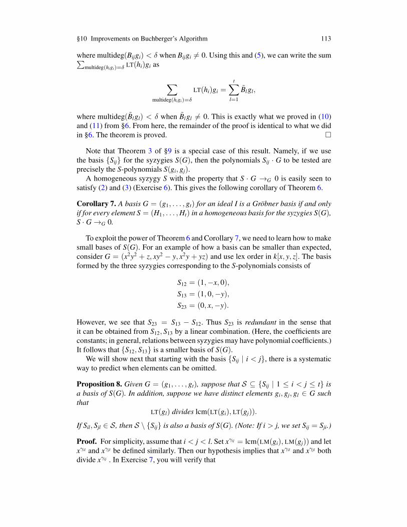
§10 Improvements on Buchberger’s Algorithm 113
where multideg(Bijgi) < δ when Bijgi = 0. Using this and (5), we can write the sum∑multideg(higi)=δ LT(hi)gi as
∑
multideg(higi)=δ
LT(hi)gi =t∑
l=1
Blgl,
where multideg(Blgl) < δ when Blgl = 0. This is exactly what we proved in (10)and (11) from §6. From here, the remainder of the proof is identical to what we didin §6. The theorem is proved. !
Note that Theorem 3 of §9 is a special case of this result. Namely, if we usethe basis {Sij} for the syzygies S(G), then the polynomials Sij · G to be tested areprecisely the S-polynomials S(gi, gj).
A homogeneous syzygy S with the property that S · G →G 0 is easily seen tosatisfy (2) and (3) (Exercise 6). This gives the following corollary of Theorem 6.
Corollary 7. A basis G = (g1, . . . , gt) for an ideal I is a Gröbner basis if and onlyif for every element S = (H1, . . . ,Ht) in a homogeneous basis for the syzygies S(G),S · G →G 0.
To exploit the power of Theorem 6 and Corollary 7, we need to learn how to makesmall bases of S(G). For an example of how a basis can be smaller than expected,consider G = (x2y2 + z, xy2 − y, x2y + yz) and use lex order in k[x, y, z]. The basisformed by the three syzygies corresponding to the S-polynomials consists of
S12 = (1,−x, 0),
S13 = (1, 0,−y),
S23 = (0, x,−y).
However, we see that S23 = S13 − S12. Thus S23 is redundant in the sense thatit can be obtained from S12, S13 by a linear combination. (Here, the coefficients areconstants; in general, relations between syzygies may have polynomial coefficients.)It follows that {S12, S13} is a smaller basis of S(G).
We will show next that starting with the basis {Sij | i < j}, there is a systematicway to predict when elements can be omitted.
Proposition 8. Given G = (g1, . . . , gt), suppose that S ⊆ {Sij | 1 ≤ i < j ≤ t} isa basis of S(G). In addition, suppose we have distinct elements gi, gj, gl ∈ G suchthat
LT(gl) divides lcm(LT(gi), LT(gj)).
If Sil, Sjl ∈ S, then S \ {Sij} is also a basis of S(G). (Note: If i > j, we set Sij = Sji.)
Proof. For simplicity, assume that i < j < l. Set xγij = lcm(LM(gi), LM(gj)) and letxγil and xγjl be defined similarly. Then our hypothesis implies that xγil and xγjl bothdivide xγij . In Exercise 7, you will verify that

114 Chapter 2 Gröbner Bases
Sij =xγij
xγilSil −
xγij
xγjlSjl,
and the proposition is proved. !To incorporate this proposition into an algorithm for creating Gröbner bases, we
will use the ordered pairs (i, j) with i < j to keep track of which syzygies we want.Since we sometimes will have an i = j where we do not know which is larger, wewill use the following notation: given i = j, define
[i, j] =
{(i, j) if i < j(j, i) if i > j.
We can now state an improved version of Buchberger’s algorithm that takes intoaccount the results proved so far.
Theorem 9. Let I = ⟨ f1, . . . , fs⟩ be a polynomial ideal. Then a Gröbner basis of Ican be constructed in a finite number of steps by the following algorithm:
Input : F = ( f1, . . . , fs)
Output : a Gröbner basis G for I = ⟨ f1, . . . , fs⟩
B := {(i, j) | 1 ≤ i < j ≤ s}G := F
t := s
WHILE B = ∅ DOSelect (i, j) ∈ B
IF lcm(LT( fi), LT( fj)) = LT( fi)LT( fj) AND
Criterion( fi, fj,B) = false THEN
r := S( fi, fj)G
IF r = 0 THEN
t := t + 1; ft := r
G := G ∪ { ft}B := B ∪ {(i, t) | 1 ≤ i ≤ t − 1}
B := B \ {(i, j)}RETURN G
Here, Criterion( fi, fj,B) is true provided that there is some l /∈ {i, j} for which thepairs [i, l] and [ j, l] are not in B and LT( fl) divides lcm(LT( fi), LT( fj)). (Note thatthis criterion is based on Proposition 8.)
Proof. The basic idea of the algorithm is that B records the pairs (i, j) that remain tobe considered. Furthermore, we only compute the remainder of those S-polynomialsS(gi, gj) for which neither Proposition 1 nor Proposition 8 applies.
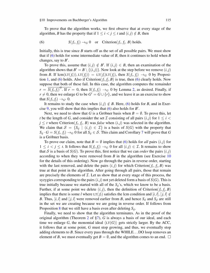
§10 Improvements on Buchberger’s Algorithm 115
To prove that the algorithm works, we first observe that at every stage of thealgorithm, B has the property that if 1 ≤ i < j ≤ t and (i, j) /∈ B, then
(6) S( fi, fj) →G 0 or Criterion( fi, fj, B) holds.
Initially, this is true since B starts off as the set of all possible pairs. We must showthat if (6) holds for some intermediate value of B, then it continues to hold when Bchanges, say to B′.
To prove this, assume that (i, j) /∈ B′. If (i, j) ∈ B, then an examination of thealgorithm shows that B′ = B \ {(i, j)}. Now look at the step before we remove (i, j)from B. If lcm(LT( fi)), LT( fj)) = LT( fi)LT( fj), then S( fi, fj) →G 0 by Proposi-tion 1, and (6) holds. Also if Criterion( fi, fj,B) is true, then (6) clearly holds. Nowsuppose that both of these fail. In this case, the algorithm computes the remainderr = S( fi, fj)
G. If r = 0, then S( fi, fj) →G 0 by Lemma 2, as desired. Finally, if
r = 0, then we enlargeG to be G′ = G∪ {r}, and we leave it as an exercise to showthat S( fi, fj) →G′ 0.
It remains to study the case when (i, j) /∈ B. Here, (6) holds for B, and in Exer-cise 9, you will show that this implies that (6) also holds for B′.
Next, we need to show that G is a Gröbner basis when B = ∅. To prove this, lett be the length of G, and consider the set I consisting of all pairs (i, j) for 1 ≤ i <j ≤ t where Criterion( fi, fj, B) was false when (i, j) was selected in the algorithm.We claim that S = {Sij | (i, j) ∈ I} is a basis of S(G) with the property thatSij ·G = S( fi, fj) →G 0 for all Sij ∈ S. This claim and Corollary 7 will prove that Gis a Gröbner basis.
To prove our claim, note that B = ∅ implies that (6) holds for all pairs (i, j) for1 ≤ i < j ≤ t. It follows that S( fi, fj) →G 0 for all (i, j) ∈ I. It remains to showthat S is a basis of S(G). To prove this, first notice that we can order the pairs (i, j)according to when they were removed from B in the algorithm (see Exercise 10for the details of this ordering). Now go through the pairs in reverse order, startingwith the last removed, and delete the pairs (i, j) for which Criterion( fi, fj,B) wastrue at that point in the algorithm. After going through all pairs, those that remainare precisely the elements of I. Let us show that at every stage of this process, thesyzygies corresponding to the pairs (i, j) not yet deleted form a basis of S(G). This istrue initially because we started with all of the Sij’s, which we know to be a basis.Further, if at some point we delete (i, j), then the definition of Criterion( fi, fj,B)implies that there is some l where LT( fl) satisfies the lcm condition and [i, l], [ j, l] /∈B. Thus, [i, l] and [ j, l] were removed earlier from B, and hence Sil and Sjl are stillin the set we are creating because we are going in reverse order. If follows fromProposition 8 that we still have a basis even after deleting Sij.
Finally, we need to show that the algorithm terminates. As in the proof of theoriginal algorithm (Theorem 2 of §7), G is always a basis of our ideal, and eachtime we enlarge G, the monomial ideal ⟨LT(G)⟩ gets strictly larger. By the ACC,it follows that at some point, G must stop growing, and thus, we eventually stopadding elements to B. Since every pass through the WHILE. . .DO loop removes anelement of B, we must eventually get B = ∅, and the algorithm comes to an end. !

116 Chapter 2 Gröbner Bases
The algorithm given above is still not optimal, and several strategies have beenfound to improve its efficiency further. For example, in the division algorithm (Theo-rem 3 of §3), we allowed the divisors f1, . . . , fs to be listed in any order. In practice,some effort could be saved on average if we arranged the fi so that their leadingterms are listed in increasing order with respect to the chosen monomial ordering.Since the smaller LT( fi) are more likely to be used during the division algorithm,listing them earlier means that fewer comparisons will be required. A second strat-egy concerns the step where we choose (i, j) ∈ B in the algorithm of Theorem 9.BUCHBERGER (1985) suggests that there will often be some savings if we pick(i, j) ∈ B such that lcm(LM( fi), LM( fj)) is as small as possible. The correspondingS-polynomials will tend to yield any nonzero remainders (and new elements of theGröbner basis) sooner in the process, so there will be more of a chance that subse-quent remainders S( fi, fj)
Gwill be zero. This normal selection strategy is discussed
in more detail in BECKER and WEISPFENNING (1993), BUCHBERGER (1985) andGEBAUER and MÖLLER (1988). Finally, there is the idea of sugar, which is a re-finement of the normal selection strategy. Sugar and its variant double sugar can befound in GIOVINI, MORA, NIESI, ROBBIANO and TRAVERSO (1991).
In another direction, one can also modify the algorithm so that it will automati-cally produce a reduced Gröbner basis (as defined in §7). The basic idea is to sys-tematically reduce G each time it is enlarged. Incorporating this idea also generallylessens the number of S-polynomials that must be divided in the course of the algo-rithm. For a further discussion of this idea, consult BUCHBERGER (1985).
We will discuss further ideas for computing Gröbner bases in Chapter 10.
Complexity Issues
We will end this section with a short discussion of the complexity of computingGröbner bases. Even with the best currently known versions of the algorithm, it isstill easy to generate examples of ideals for which the computation of a Gröbnerbasis takes a tremendously long time and/or consumes a huge amount of storagespace. There are several reasons for this:• The total degrees of intermediate polynomials that must be generated as the al-
gorithm proceeds can be quite large.• The coefficients of the elements of a Gröbner basis can be quite complicated
rational numbers, even when the coefficients of the original ideal generators weresmall integers. See Example 3 of §8 or Exercise 13 of this section for someinstances of this phenomenon.
For these reasons, a large amount of theoretical work has been done to try to es-tablish uniform upper bounds on the degrees of the intermediate polynomials inGröbner basis calculations when the degrees of the original generators are given. Forsome specific results in this area, see DUBÉ (1990) and MÖLLER and MORA (1984).The idea is to measure to what extent the Gröbner basis method will continue to betractable as larger and larger problems are attacked.

§10 Improvements on Buchberger’s Algorithm 117
The bounds on the degrees of the generators in a Gröbner basis are quite large,and it has been shown that large bounds are necessary. For instance, MAYR andMEYER (1982) give examples where the construction of a Gröbner basis for anideal generated by polynomials of degree less than or equal to some d can involvepolynomials of degree proportional to 22
d. As d → ∞, 22
dgrows very rapidly. Even
when grevlex order is used (which often gives the smallest Gröbner bases—seebelow), the degrees can be quite large. For example, consider the polynomials
xn+1 − yzn−1w, xyn−1 − zn, xnz− ynw.
If we use grevlex order with x > y > z > w, then Mora [see LAZARD (1983)]showed that the reduced Gröbner basis contains the polynomial
zn2+1 − yn
2w.
The results led for a time to some pessimism concerning the ultimate practicalityof the Gröbner basis method as a whole. Further work has shown, however, thatfor ideals in two and three variables, much more reasonable upper degree boundsare available [see, for example, LAZARD (1983) and WINKLER (1984)]. Further-more, in any case the running time and storage space required by the algorithmseem to be much more manageable “on average” (and this tends to include mostcases of geometric interest) than in the worst cases. There is also a growing real-ization that computing “algebraic” information (such as the primary decompositionof an ideal—see Chapter 4) should have greater complexity than computing “geo-metric” information (such as the dimension of a variety—see Chapter 9). A goodreference for this is GIUSTI and HEINTZ (1993), and a discussion of a wide varietyof complexity issues related to Gröbner bases can be found in BAYER and MUM-FORD (1993). See also pages 616–619 of VON ZUR GATHEN and GERHARD (2013)for further discussion and references.
Finally, experimentation with changes of variables and varying the ordering ofthe variables often can reduce the difficulty of the computation drastically. BAYER
and STILLMAN (1987a) have shown that in most cases, the grevlex order shouldproduce a Gröbner basis with polynomials of the smallest total degree. In a differentdirection, it is tempting to consider changing the monomial ordering as the algo-rithm progresses in order to produce a Gröbner basis more efficiently. This idea wasintroduced in GRITZMANN and STURMFELS (1993) and has been taken up again inCABOARA and PERRY (2014).
EXERCISES FOR §10
1. Let S = (c1, . . . , cs) and T = (d1, . . . , ds) ∈ (k[x1, . . . , xn])s be syzygies on the leadingterms of F = ( f1, . . . , fs).a. Show that S+ T = (c1 + d1, . . . , cs + ds) is also a syzygy.b. Show that if g ∈ k[x1, . . . , xn], then g · S = (gc1, . . . , gcs) is also a syzygy.
2. Given any G = (g1, . . . , gs) ∈ (k[x1, . . . , xn])s , we can define a syzygy on G to be an s-tuple S = (h1, . . . , hs) ∈ (k[x1, . . . , xn])s such that
∑i higi = 0. [Note that the syzygies
we studied in the text are syzygies on LT(G) = (LT(g1), . . . , LT(gs)).]

118 Chapter 2 Gröbner Bases
a. Show that if G = (x2 − y, xy− z, y2 − xz), then (z,−y, x) defines a syzygy on G.b. Find another syzygy on G from part (a).c. Show that if S, T are syzygies on G, and g ∈ k[x1, . . . , xn], then S+T and gS are also
syzygies on G.3. LetM be an m× (m+ 1) matrix of polynomials in k[x1, . . . , xn]. Let I be the ideal gen-
erated by the determinants of all the m× m submatrices of M (such ideals are examplesof determinantal ideals).a. Find a 2×3 matrixM such that the associated determinantal ideal of 2×2 submatrices
is the ideal with generators G as in part (a) of Exercise 2.b. Explain the syzygy given in part (a) of Exercise 2 in terms of your matrix.c. Give a general way to produce syzygies on the generators of a determinantal ideal.
Hint: Find ways to produce (m+ 1)× (m+ 1) matrices containing M, whose deter-minants are automatically zero.
4. Prove that the syzygy Sij defined in (1) is homogeneous of multidegree γ.5. Complete the proof of Lemma 4 by showing that the decomposition into homogeneous
components is unique. Hint: First show that if S =∑
α S′α, where S′α has multidegree
α, then, for a fixed i, the ith components of the S′α are either 0 or have multidegree equalto α−multideg( fi) and, hence, give distinct terms as α varies.
6. Suppose that S is a homogeneous syzygy of multidegree α in S(G).a. Prove that S · G has multidegree < α.b. Use part (a) to show that Corollary 7 follows from Theorem 6.
7. Complete the proof of Proposition 8 by proving the formula expressing Sij in terms ofSil and Sjl.
8. Let G be a finite subset of k[x1, . . . , xn] and let f ∈ ⟨G⟩. If f G = r = 0, then show thatf →G′ 0, where G′ = G ∪ {r}. This fact is used in the proof of Theorem 9.
9. In the proof of Theorem 9, we claimed that for every value of B, if 1 ≤ i < j ≤ t and(i, j) /∈ B, then condition (6) was true. To prove this, we needed to show that if theclaim held for B, then it held when B changed to some B′. The case when (i, j) /∈ B′ but(i, j) ∈ B was covered in the text. It remains to consider when (i, j) /∈ B′ ∪ B. In thiscase, prove that (6) holds for B′. Hint: Note that (6) holds for B. There are two casesto consider, depending on whether B′ is bigger or smaller than B. In the latter situation,B′ = B \ {(l,m)} for some (l,m) = (i, j).
10. In this exercise, we will study the ordering on the set {(i, j) | 1 ≤ i < j ≤ t} describedin the proof of Theorem 9. Assume that B = ∅, and recall that t is the length of G whenthe algorithm stops.a. Show that any pair (i, j) with 1 ≤ i < j ≤ t was a member of B at some point during
the algorithm.b. Use part (a) and B = ∅ to explain how we can order the set of all pairs according to
when a pair was removed from B.11. Consider f1 = x3−2xy and f2 = x2y−2y2+x and use grlex order on k[x, y]. These poly-
nomials are taken from Example 1 of §7, where we followed Buchberger’s algorithmto show how a Gröbner basis was produced. Redo this example using the algorithm ofTheorem 9 and, in particular, keep track of how many times you have to use the divisionalgorithm.
12. Consider the polynomials
xn+1 − yzn−1w, xyn−1 − zn, xnz − ynw,
and use grevlex order with x > y > z > w. Mora [see LAZARD (1983)] showed that thereduced Gröbner basis contains the polynomial
zn2+1 − yn
2w.
Prove that this is true when n is 3, 4, or 5. How big are the Gröbner bases?
§10 Improvements on Buchberger’s Algorithm 119
13. In this exercise, we will look at some examples of how the term order can affect thelength of a Gröbner basis computation and the complexity of the answer.a. Compute a Gröbner basis for I = ⟨x5 + y4 + z3 − 1, x3 + y2 + z2 − 1⟩ using lex and
grevlex orders with x > y > z. You will see that the Gröbner basis is much simplerwhen using grevlex.
b. Compute a Gröbner basis for I = ⟨x5 + y4 + z3 − 1, x3 + y3 + z2 − 1⟩ using lexand grevlex orders with x > y > z. This differs from the previous example by asingle exponent, but the Gröbner basis for lex order is significantly nastier (one of itspolynomials has 282 terms, total degree 25, and a largest coefficient of 170255391).
c. Let I = ⟨x4 − yz2w, xy2 − z3, x3z − y3w⟩ be the ideal generated by the polynomialsof Exercise 12 with n = 3. Using lex and grevlex orders with x > y > z > w, showthat the resulting Gröbner bases are the same. So grevlex is not always better thanlex, but in practice, it is usually a good idea to use grevlex whenever possible.