chapter 2: mechanics - weebly · an experiment in acceleration • in the early 1950s military...
TRANSCRIPT

Chapter 2: Mechanics Section 1: Motion-Kinematics
Section 2: Forces-Dynamics
Section 3: Work and Energy
Section 4: Momentum and Impulse

Section 2.1 Kinematics Study of Motion in 1 and 2-D
Recommended Practice
Questions: 3, 4, 6, 10, 14, 19, 20
Problems: 2, 4, 7, 8, 9, 11, 13, 20, 24, 26, 27, 36, 37, 39, 47, 52

Section 2.1: Kinematics Study of Motion and Projectiles
Recommended Practice Giancoli Chp 2
Questions: 3, 4, 6, 10, 14, 19, 20
Problems: 2, 4, 7, 8, 9, 11, 13, 20, 24, 26, 27, 36, 37, 39, 47, 52
Chp 3 Problems: 9, 10, 14, 18, 19, 22, 23, 24, 27, 30, 31, 33, 62

Section 1 Objectives
Core Principles
• Distance and displacement
• Speed and velocity
• Acceleration
• Graphs describing motion
• Equations of motion for uniform acceleration
• Projectile motion
• Fluid resistance and terminal speed
Applications and skills: • Determining instantaneous and average values for velocity,
speed and acceleration • Solving problems using equations of motion for uniform
acceleration • Sketching and interpreting motion graphs • Determining the acceleration of free-fall experimentally • Analysing projectile motion, including the resolution of
vertical and horizontal components of acceleration, velocity and displacement
• Qualitatively describing the effect of fluid resistance on falling objects or projectiles, including reaching terminal speed

ToK and Aims
Theory of knowledge:
The independence of horizontal and vertical motion in projectile motion seems to be counter-intuitive. How do scientists work around their intuitions? How do scientists make use of their intuitions?
Aims:
• Aim 2: much of the development of classical physics has been built on the advances in kinematics
• Aim 6: experiments, including use of data logging, could include (but are not limited to): determination of g, estimating speed using travel timetables, analysing projectile motion, and investigating motion through a fluid
• Aim 7: technology has allowed for more accurate and precise measurements of motion, including video analysis of real-life projectiles and modelling/simulations of terminal velocity
Historical Perspective of Mechanics
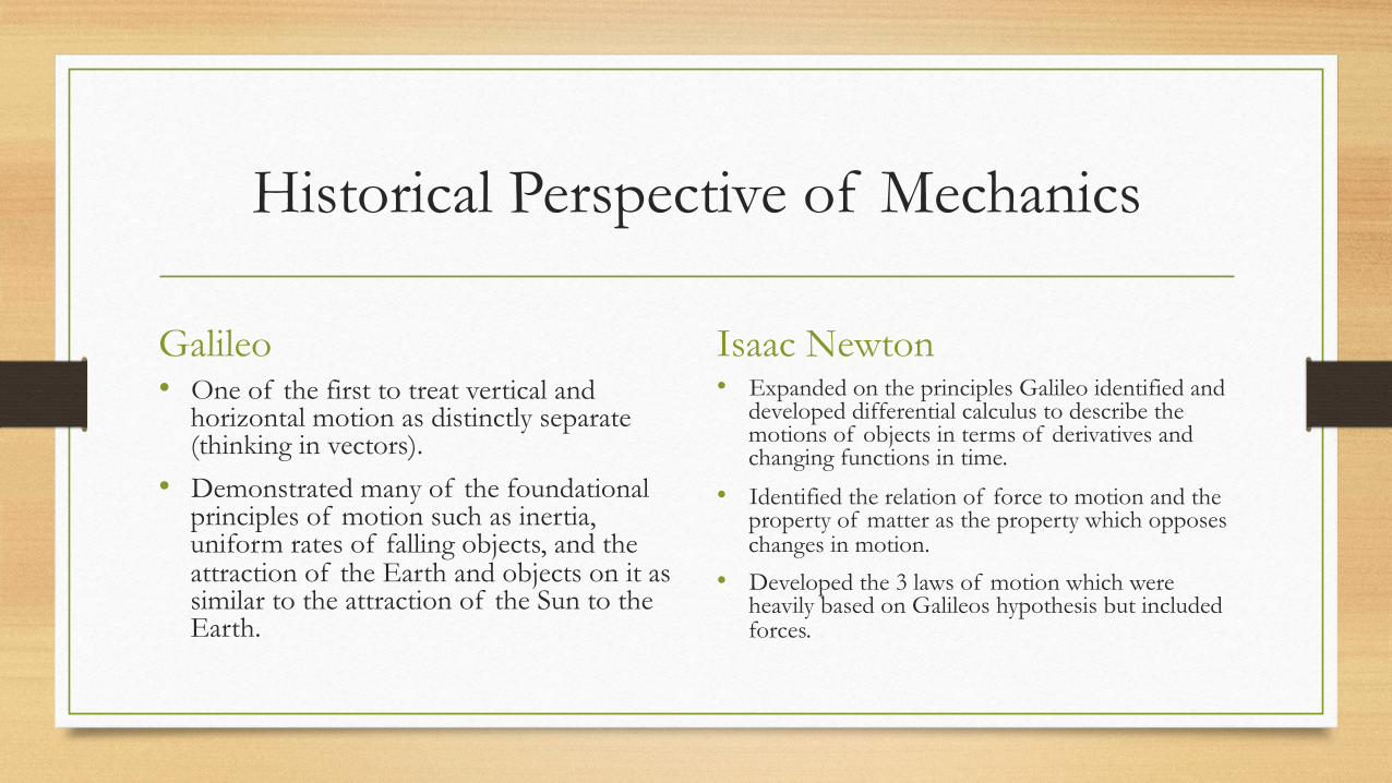
Galileo • One of the first to treat vertical and
horizontal motion as distinctly separate (thinking in vectors).
• Demonstrated many of the foundational principles of motion such as inertia, uniform rates of falling objects, and the attraction of the Earth and objects on it as similar to the attraction of the Sun to the Earth.
Isaac Newton • Expanded on the principles Galileo identified and
developed differential calculus to describe the motions of objects in terms of derivatives and changing functions in time.
• Identified the relation of force to motion and the property of matter as the property which opposes changes in motion.
• Developed the 3 laws of motion which were heavily based on Galileos hypothesis but included forces.

Kinematics
Study of Motion Essential idea: Motion may be described and
analyzed by the use of graphs and equations.
Nature of science: Observations: The ideas of motion are fundamental to many areas of physics, providing a link to the consideration of forces and their implication. The kinematic equations for uniform acceleration were developed through careful observations of the natural world.
Utilization: Diving, parachuting and similar activities where fluid resistance affects motion • The accurate use of ballistics requires careful analysis • Biomechanics (see Sports, exercise and health science SL sub-topic 4.3) • Quadratic functions (see Mathematics HL sub-topic 2.6; Mathematics SL sub-topic 2.4; Mathematical studies SL sub-topic 6.3) • The kinematic equations are treated in calculus form in Mathematics HL sub-topic 6.6 and Mathematics SL sub-topic 6.6

Position (denoted X or Y) Kinematics is the study of displacement, velocity and acceleration, or in short, a study of motion.
•A study of motion begins with position and change in position.
Defining position
(1) Distance: how far an object has traveled, without regard to point of origin or direction of travel (scalar quantity)
(2) Displacement: how far an object has traveled with respect to a point of origin, direction matters (vector quantity)
Remember our discussions of vectors, positive and negative are useful ways to describe changes position in 1 dimension but falls into trouble when the vectors are multidimensional.
Ex: What is the
Distance?
Displacement?
Origin 3m 10m

Distance vs Displacement
Let us assume that a ball rests on a track. If every colored segment represents 1m answer the following:
If the ball starts at
Position 1 and then moves to position 2, what is the distance traveled? The displacement?
Now if it travels from position 2 to position 3 what is the total distance traveled? The total displacement?
•Now for some detailed analysis of these two motions… •Displacement ∆x (or s) has the following formulas:
displacement ∆x = x2 – x1 s = x2 – x1
where x2 is the final position and x1 is the initial position
x(m) 1
x(m)
2
2 3

Changes in Position in Time
• Using the previous example, say that the ball traveled the first leg (from 1 to 2) in 3 seconds. Now assume that it traveled from 2 to 3 in 5 seconds.
• Graph this motion with the position on the y axis and the time on the x axis (let time start when the ball starts rolling so initially t=0).
• Note that the slope of the line for the position/time graph is gained by using m = 𝑥↓𝑓 − 𝑥↓𝑖 /𝑡↓𝑓 − 𝑡↓𝑖 this
equation can be written in terms of changes in x and t using delta notation, then v = Δ𝑥/Δ𝑡 is the rate at which the ball moves.
• The physical quantity for the rate an object moves through a displacement is Velocity.
• Then we have calculated the average velocity of the ball through each segment of its motion. How does this value change if we take the average over the entire duration?

Velocity and Speed
• Here we have a Displacement/time graph. Find the average
velocity from t=0 to t=10s. Do the same for t=15 to 30s. • What is the sign of the two slopes telling us?
• Find the average velocity from t=0 to t=30s. Now find the average speed from t=0 to t=30s.
• Why are they different?
Dis
plac
emen
t (m
)
Time (s)

Changes in Velocity in time
• A car is traveling 20ms-1 down the road. If it does so for 15 seconds how far has it traveled?
• Now, draw the velocity/time plot for a car which is initially traveling 20ms-1 for 5 seconds, slows down steadily to a very brief stop after 3 seconds, then smoothly reverses to -5ms-1 over the next 8 seconds and then maintains that velocity for the next 4 seconds.
• Find the slope of the velocity curve for each distinct line segment using the same slope formula as for the position time
graph m = 𝑣↓𝑓 − 𝑣↓𝑖 /𝑡↓𝑓 − 𝑡↓𝑖 . • You can re-write this in delta notation just as previously, a = Δ𝑣/Δ𝑡 then we have calculated the average acceleration for the car
during these times. What is the derived unit for acceleration?
• Lastly, find the area under the entire curve (t=0 to t=20s)
• (Hint: Don’t forget to write units when you perform the calculations)
• What have you found when you computed this area?

Average and Instantaneous Velocity
• We can label each position with an x and the time interval between each x with a ∆t.
• Then vA = (x2 - x1)/∆t, vB = (x3 - x2)/∆t, and finally vC = (x4 - x3)/∆t.
• Focus on the interval from x2 to x3.
• Note that the speed changed from x2 to x3, and so vB is NOT really the speed for that whole interval.
• We say the vB is an average speed (as are vA and vC).
x1 x2 x3 x4
∆t ∆t ∆t vA vB vC

An Experiment in Acceleration • In the early 1950s military aeronautical engineers
were researching the effects of acceleration on the human body and were concluding (without much evidence) that the human body couldn’t survive the stress of a rapid ejection system and so put little emphasis on pilot safety belts and ejection seats (assuming that the conditions of the ejection would be roughly as lethal as the crash).
• Colonel Stapp, and air force physician decided that the assumptions were not not valid and proposed to determine the effects of high accelerations on the body.
• A rocket sled was designed to accelerate up to 40gs (40 times the felt force of gravity)
• Stapp had himself launched down the track and a video of the procedure taken.

Acceleration Practice
• In 1954, America's original Rocketman, Col. John Paul Stapp, attained a then-world record land speed of 632 mph, going from a standstill to a speed faster than a .45 bullet in 5.0 seconds on an especially-designed rocket sled, and then screeched to a dead stop in 1.4 seconds, sustaining more than 40g's of force, all in the interest of safety.
• There are TWO accelerations in this problem calculate the acceleration both when
(a) He speeds up from 0 to 632 mph in 5.0 s.
(b) He slows down from 632 mph to 0 in 1.4 s.
Calculate the two accelerations, in ms-2. Put these in gs (1g=10ms2). Which one is larger?

Equations of Motion
We have then established the 3 foundational relationships on which motion is based:
Position is defined as a displacement from an initial position.
Velocity is defined as the rate of change of displacement in time. Acceleration is defined as the rate of change of velocity in time.
From these we can produce our kinematic equations after a little derivation and under a very specific condition: acceleration must be constant Firstly remember our first principles v = 𝒙↓𝒇 − 𝒙↓𝒊 /𝒕↓𝒇 − 𝒕↓𝒊 v = Δ𝑥/Δ𝑡 and a = 𝒗↓𝒇 − 𝒗↓𝒊 /𝒕↓𝒇 − 𝒕↓𝒊 a = Δ𝑣/Δ𝑡

Kinematic Equation for Velocity
• Given that we know a = 𝑣↓𝑓 − 𝑣↓𝑖 /𝑡↓𝑓 − 𝑡↓𝑖 , and, if we let the initial time be 0 we can simply call 𝑡↓𝑓 − 𝑡↓𝑖 t, the time of interest, then a = 𝑣↓𝑓 − 𝑣↓𝑖 /𝑡 .
• Then we can multiply by t and get at = 𝑣↓𝑓 − 𝑣↓𝑖 . At this point if we want an equation for the final velocity, given the initial velocity, a constant acceleration, and time, we have
vf = vi + at
our velocity equation in terms of time and acceleration.

Kinematic Equations for Position
• Firstly we know by the first principles that xf = xi + vt. This is the starting point for our displacement equation if we have no acceleration.
• Now, if we know that our displacement x = xf – xi and that, for a constant acceleration, the velocity can be calculated by taking an average of the first and last velocity for that period, then the average velocity is 𝒗 = 𝒗↓𝒇 + 𝒗↓𝒊 /𝟐
• Then substitute to get the equation for average position: xf = xi + [𝒗↓𝒇 + 𝒗↓𝒊 /𝟐 ]t • Now if we substitute our velocity equation earlier vf = vi + at into this equation we obtain
• xf = xi + [𝑣↓𝑖 + at + 𝑣↓𝑖 /2 ]t • We can then simplify this equation to produce
• xf = xi + 𝒗↓𝒊 t + 𝒂𝒕↑𝟐 /𝟐 • This is our general Displacement/Position equation for a uniform acceleration.

Time Independent Velocity Equation
• Now that we have our equations for position and velocity let us perform an algebraic manipulation to get a shortcut equation for velocity if we don’t have time:
• Start with xf = xi + 𝑣 t and vf = vi + at; Now solve the velocity equation for time: t = 𝑣↓𝑓 − 𝑣↓𝑖 /𝑎 • Now substitute this value of t into our position equation xf = xi + 𝒗 t • Then xf = xi +[ 𝑣↓𝑓 + 𝑣↓𝑖 /2 ] [𝑣↓𝑓 − 𝑣↓𝑖 /𝑎 ] • From this we can use algebra to manipulate the equation into the following form
(xf – xi)·2a = (𝑣↓𝑓 + 𝑣↓𝑖 )(𝑣↓𝑓 − 𝑣↓𝑖 ) • If we foil this right side we find that we have a difference of perfect squares and the cross terms cancel to produce
(xf – xi)·2a = 𝑣↓𝑓 2 - 𝑣↓𝑖 2 • We can then solve this equation for the final velocity to obtain our equation for velocity without needing time.
vf2 = vi
2 + 2a(xf – xi)

4 Kinematic Equations
• Then we have produced our 4 major kinematic equations
Average Displacement: xf = xi + 𝒗 t ; 𝒗 = 𝒗↓𝒊 + 𝒗↓𝒇 /𝟐 Displacement: xf = xi + 𝒗↓𝒊 t + 𝒂𝒕↑𝟐 /𝟐 Velocity (with time): vf = vi + at
Velocity (timeless): vf2 = vi
2 + 2a(xf – xi)

Falling Objects
• As has been discussed before and in previous examples, our kinematic equations require constant acceleration.
• The most common case for this is for falling objects. A falling object (or object thrown directly up) has only the force of gravity causing it to accelerate.
• The acceleration due to gravity at the Earth’s surface is so common we call it g and g= 9.8ms-2 towards the ground.
• Then our kinematic equations for falling objects take on the form
yf = yi + 𝒗 t ; 𝒗 = 𝒗↓𝒊 + 𝒗↓𝒇 /𝟐 ; yf = yi + 𝒗↓𝒊 t - 𝒈𝒕↑𝟐 /𝟐 vf = vi - gt
vf2 = vi
2 – 2g(yf – yi)

-35
-30
-25
-20
-15
-10
-5
0 0 0.5 1 1.5 2 2.5 3 3.5
Vel
ocity
in Y
(ms-1
)
Time (s)
Velocity Time Plot of Falling Object
Plotting the Trajectory of a Falling Object
• Consider the displacement of a dropped object, shown by the figures and graph
• Using the information provided find the equation which generates this graph.
• What initial information is needed or assumed?
• Using what you know about the relationships between acceleration, velocity, and position, what should the graph of velocity look like?
-50
-45
-40
-35
-30
-25
-20
-15
-10
-5
0 0 0.5 1 1.5 2 2.5 3 3.5
Posi
tion
in Y
(m)
Time (s)
Position Time Graph for Falling Object

Plotting the Trajectory of an Object Thrown Straight Up
• Previously we worked with the case that the initial velocity of the object was 0.
• If we now give the object some initial velocity in the positive direction, describe the arrow diagram for motion. Estimate the trajectory.
• Now let’s use a specific example
• For a ball launched straight up from the ground at 15ms-1 list our knowns:
• yi = ?
• vi = ?
• a = ?
• Let us generate the table of values we need to plot the trajectory, if we record the position every 0.2seconds.
• What function will give us this data easily?
Time (s) Position (m)0 0.0
0.2 2.80.4 5.20.6 7.20.8 8.9
1 10.11.2 10.91.4 11.41.6 11.51.8 11.1
2 10.42.2 9.32.4 7.82.6 5.92.8 3.6
3 0.9
0.0
2.0
4.0
6.0
8.0
10.0
12.0
14.0
0 0.5 1 1.5 2 2.5 3 3.5
Posi
tion
in Y
(m)
Time (s)
Trajectory

Terminal Velocity and Air Resistance
• Generally we try to ignore air resistance, because air resistance is an external force which causes acceleration to change and invalidates our kinematic equations.
• As an object falls and gains velocity the friction between the object and the air increases (air is a fluid and resists motion through it).
• This is known as Drag or Air resistance and is α v2 then as the object falls it experiences greater resistance to its motion and slows.
• When Fdrag = Fgravity the forces balance and the object no longer accelerates, thus its velocity has become constant.
• This velocity is known as the Terminal Velocity of the object.

Relative Velocity and Vectors
• Up until now we have restricted our discussion of kinematics to a single object moving in 1-D.
• However, objects are frequently moving in at least two spatial dimensions (including time in each) and there are often more than one object involved in the situation.
• Ex: cars in traffic. If you have two cars moving at different velocities then they are both moving with a certain velocity compared to a person at rest, that is what we mean when we say that our choice of reference points or inertial frames is important. If car 1 has velocity 50mph down the street and car 2 has velocity 35mph in the same direction, then how fast is car 1 going compared to car 2?
• This process is known as finding relative velocity and for 2 vectors A and B
VAB = VA - VB
• Try the same situation only car 1 is moving 50mph; 0° while car 2 has velocity 35mph; 270°. Use vector subtraction to find the relative velocity. (Draw the vector diagram!)

Practice

Kinematics in 2-D (Projectile Motion)
• One of the most simple cases of objects moving in 2-D is the case of a projectile.
• Projectile motion: the motion of an object which has been given an initial velocity and is subsequently under no other influence than gravity.
• A projectile then has motion in X and Y axis. It is important to remember how to use our vector knowledge to separate the motion of a projectile into its independent X and Y motions.

Compare the Ball Dropped and Rolled off a Table • To make the situation clear let us compare these two scenarios. Remember the 1-D motion of a dropped ball earlier:
t1 =0
t2 =.5
t3 =1
t4 =1.5
t5 =2
t6 =2.5
x=0, y=0; vx=0 vy=0; ax=0, ay=-g
x=0, y=−g𝑡↓2 ↑2 /2 ; vx=0 vy=-gt2 ; ax=0, ay=-g x=0, y=−g𝑡↓3 ↑2 /2 ; vx=0 vy=-gt3 ; ax=0, ay=-g
x=0, y=−g𝑡↓4 ↑2 /2 ; vx=0 vy=-gt4 ; ax=0, ay=-g
x=0, y=−g𝑡↓5 ↑2 /2 ; vx=0 vy=-gt5 ; ax=0, ay=-g
x=0, y=−g𝑡↓6 ↑2 /2 ; vx=0 vy=-gt6 ; ax=0, ay=-g
t1 =0
t2 =.5
t3 =1
t4 =1.5
t5 =2
t6 =2.5
x=0, y=0; vx=0 vy=0; ax=0, ay=-g
x=vxt2 , y=−g𝑡↓2 ↑2 /2 ; vx=0 vy=-gt2 ; ax=0, ay=-g
Ball Dropped Ball Rolled off Table
x=vxt3 , y=−g𝑡↓3 ↑2 /2 ; vx=0 vy=-gt3 ; ax=0, ay=-g
x=vxt4 , y=−g𝑡↓4 ↑2 /2 ; vx=0 vy=-gt4 ; ax=0, ay=-g
x=vxt5 , y=−g𝑡↓5 ↑2 /2 ; vx=0 vy=-gt5 ; ax=0, ay=-g
x=vxt6 , y=−g𝑡↓6 ↑2 /2 ; vx=0 vy=-gt6 ; ax=0, ay=-g

Separation of Components and Vector Form of Motion Equations
• Then the usefulness of vectors is made apparent. In order to do 2-D kinematics we only have to do 1-D kinematics twice. All of our methods we previously used still work, we just have to apply them to the x and y vector components. Then we can write our equations for displacement, velocity and acceleration as 2-D vectors with their components being the displacement and velocity equations we previously derived:
• Displacement: 𝒅 =⟨𝒙 , 𝒚 ⟩; 𝒅 =⟨xi + 𝒗↓𝒊𝒙 t, yi + 𝒗↓𝒊𝒚 t − 𝒈𝒕↑𝟐 /𝟐 ⟩ • Velocity: 𝒗 =⟨𝒗↓𝒙 , 𝒗↓𝒚 ⟩; 𝒗 =⟨𝒗↓𝒊𝒙 , 𝒗↓𝒊𝒚 − 𝒈𝒕⟩ • Acceleration: 𝒂 =⟨𝒂↓𝒙 , 𝒂↓𝒚 ⟩= ⟨𝟎,−𝒈⟩

Kinematic Equations for Projectiles
• This allows us to resolve our kinematic equations into their components.
• This table is from Giancoli and you should become comfortable working with these equations and understanding when to apply them.
• Bring your computers tomorrow!!

Describing Projectile Motion Graphically
• As we previously showed, projectile motion shares many similarities to motion of objects falling or thrown straight up, with the exception that they also include a horizontal component. Graphically then you can plot the motion of a projectile using an X(t) and Y(t) plot.
• For a projectile with an initial velocity vector 𝑣↓𝑖 = 20ms-1; 30° let us determine what our displacement and velocity equations should look like in x and y respectively, generate their t tables using those equations, and then graph them in time. It is useful here to resolve the initial velocity into its components.
X Equations xf = xi + 𝒗↓𝒊𝒙 t 𝒗↓𝒙 =𝒗↓𝒊𝒙 Ax= 0 Y Equations yf =yi + 𝒗↓𝒊𝒚 t − 𝒈𝒕↑𝟐 /𝟐 𝒗↓𝒚 =𝒗↓𝒊𝒚 - gt Ay= -g 𝒗↓𝒇𝒚 2 = 𝒗↓𝒊𝒚 2 -2g(yf – yi)
Time (s) X(m) Y(m)0.0 0.0 0.00.2 3.1 2.40.4 6.1 4.40.6 9.2 6.00.8 12.2 7.21.0 15.3 8.01.2 18.4 8.41.4 21.4 8.51.6 24.5 8.11.8 27.5 7.32.0 30.6 6.2
0.0
10.0
20.0
30.0
40.0
0.0 0.5 1.0 1.5 2.0 2.5
Dis
plac
emen
t (m
)
Time (s)
Object Motion in X
0.0 1.0 2.0 3.0 4.0 5.0 6.0
0.0 0.5 1.0 1.5 2.0 2.5
Dis
plac
emen
t (m
)
Time (s)
Object motion in Y
Deriving the Trajectory Equation
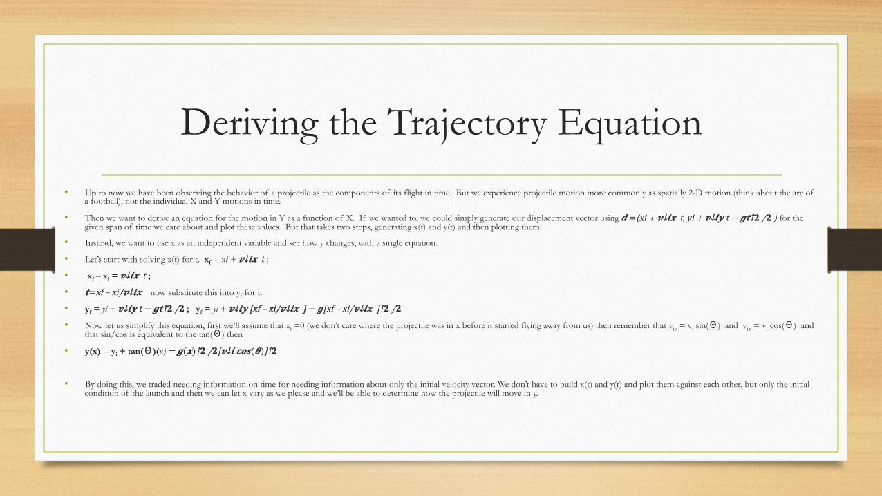
• Up to now we have been observing the behavior of a projectile as the components of its flight in time. But we experience projectile motion more commonly as spatially 2-D motion (think about the arc of a football), not the individual X and Y motions in time.
• Then we want to derive an equation for the motion in Y as a function of X. If we wanted to, we could simply generate our displacement vector using 𝒅 =⟨xi + 𝒗↓𝒊𝒙 t, yi + 𝒗↓𝒊𝒚 t − 𝒈𝒕↑𝟐 /𝟐 ⟩ for the given span of time we care about and plot these values. But that takes two steps, generating x(t) and y(t) and then plotting them.
• Instead, we want to use x as an independent variable and see how y changes, with a single equation.
• Let’s start with solving x(t) for t. xf = xi + 𝒗↓𝒊𝒙 t ;
• xf – xi = 𝒗↓𝒊𝒙 t ;
• 𝒕= xf – xi/𝒗↓𝒊𝒙 now substitute this into yf for t.
• yf = yi + 𝒗↓𝒊𝒚 t − 𝒈𝒕↑𝟐 /𝟐 ; yf = yi + 𝒗↓𝒊𝒚 [xf – xi/𝒗↓𝒊𝒙 ] − 𝒈[xf – xi/𝒗↓𝒊𝒙 ]↑𝟐 /𝟐
• Now let us simplify this equation, first we’ll assume that xi =0 (we don’t care where the projectile was in x before it started flying away from us) then remember that viy = vi sin(Θ) and vix = vi cos(Θ) and that sin/cos is equivalent to the tan(Θ) then
• y(x) = yi + tan(Θ)(x) − 𝒈(𝒙)↑𝟐 /𝟐 [𝒗↓𝒊 𝒄𝒐𝒔(𝜽)]↑𝟐
• By doing this, we traded needing information on time for needing information about only the initial velocity vector. We don’t have to build x(t) and y(t) and plot them against each other, but only the initial condition of the launch and then we can let x vary as we please and we’ll be able to determine how the projectile will move in y.

Graphing the Trajectory of a Projectile • Let us use the same information as in our previous example. The
projectile was launched at 20ms-1 at 30° from the ground. Then let us generate our y(x) function.
• vix = 20cos(30°) = 17.3ms-1;
• viy = 20cos(30°) = 10ms-1;
• if we launch from the ground then yi = 0. Then our function looks like
• y(x) = yi + tan(Θ)(x) − 𝒈(𝒙)↑𝟐 /𝟐 [𝒗↓𝒊 𝒄𝒐𝒔(𝜽)]↑𝟐
• y(x) = tan(30°)(x) − 𝒈(𝒙)↑𝟐 /𝟐 [𝟐𝟎𝒄𝒐𝒔(30°)]↑𝟐
• y(x) = .58(x) – 𝟒.𝟗 (𝒙)↑𝟐 /[𝟏𝟕.𝟑]↑𝟐
• If we want to determine how far the projectile will travel in x we can solve this quadratic equation and determine the zeros or roots.
• Remember that quad form is x = -b ± √𝑏↑2 −4𝑎𝑐 /2𝑎 then our trajectory has terms A = - 𝟒.𝟗/[𝟏𝟕.𝟑]↑𝟐 ; B = 0.58; and C = 0. Find the zeros.
• Once that is known let’s create a t-table using values from initial to final position in x by 5s.
X (m) Y (m)0 05 2.4907510 4.16315 5.0167520 5.05225 4.2687530 2.66735 0.24675
y = -0.0164x2 + 0.58x - 9E-15
-1
0
1
2
3
4
5
6
0 5 10 15 20 25 30 35 40
Y D
ispl
acem
ent (
m)
X Displacement (m)
2-D Trajectory of a Projectile

Deriving the Level Range Equation
• It’s useful to be able to find our maximum height for a projectile either by solving for the position in y for which vy is zero or by completing the square for the vertex of either the y(t) or y(x) position functions.
• But we’d also like to quickly determine the maximum range or distance in x for a projectile. In order to do this let’s first recall the condition for a projectile to remain in the air: y > 0. Then the locations where y = 0 are the locations where the projectile has stopped traveling.
• If the displacement equation in y is yf = yi + 𝒗↓𝒊𝒚 t − 𝒈𝒕↑𝟐 /𝟐 and we fire from level ground (assume yi = 0) then the range is the location in x for the time t we get from solving y(t) for the roots.
• In other words first let 0 = 𝒗↓𝒊𝒚 t − 𝒈𝒕↑𝟐 /𝟐 be the condition to be in the air. We can use the quadratic equation but, thanks to our C term being 0 we have a shortcut
• 0 = t( 𝒗↓𝒊𝒚 − 𝒈𝒕/𝟐 ); then t = 0 and 0 = 𝒗↓𝒊𝒚 − 𝒈𝒕/𝟐 are our roots. Solve for t.
• 𝒈𝒕/𝟐 = 𝒗↓𝒊𝒚 ; t = 𝟐 𝒗↓𝒊𝒚 /𝒈 ; Now we can substitute this value of t into the equation for x(t) and remember that xi is 0.
• Then xf = xi + 𝒗↓𝒊𝒙 t; xf = 𝒗↓𝒊𝒙 [𝟐 𝒗↓𝒊𝒚 /𝒈 ]
• This is then the Range equation in its most basic form. It is frequently beneficial to re-write this equation in terms of the initial velocity vector though. Remember that viy = vi sin(Θ) and vix = vi cos(Θ)
• R = 𝒗↓𝒊𝒙 [𝟐 𝒗↓𝒊𝒚 /𝒈 ]; R =2𝑣↓𝑖↑2 𝒔𝒊𝒏(𝜽)𝒄𝒐𝒔(𝜽) /𝑔 By using the trig identity 2sin(X)cos(X)=sin(2X) we arrive at our final range equation
• R= 𝒗↓𝒊↑𝟐 𝒔𝒊𝒏(𝟐𝜽)/𝒈

Cannon Example and IB Practice
• PRACTICE: A cannon fires a projectile with a muzzle velocity of 56 ms-1 at an angle of inclination of 15º.
• (a) What are vix and viy? (remember that in IB terms this is ux and uy)
• (b) What are the tailored equations of motion?
• (c) When will the ball reach its maximum height?
• (d) How far from the muzzle will the ball be when it reaches the height of the muzzle at the end of its trajectory?
• (e) Sketch the following graphs:
a vs. t, vx vs. t; vy vs. t x vs. t; y vs. t; and y(x)

More IB Sample Questions

Even More IB Test Questions

Section 2.2: Dynamics Force and Free Body Diagrams
Recommended Practice Giancoli Chp 4
Questions: 2, 3, 9, 13, 17
Problems: 2, 3, 5, 6, 9, 16, 19, 25, 27, 32, 41, 45, 52, 58, 64

Section 2 Objectives
Core Principles • Mass as a property of matter
• Objects as point particles
• Free-body diagrams
• Translational equilibrium
• Newton’s laws of motion
• Solid friction
• Motion in Circles and Centripetal Forces
• Gravitational Force and Satellites
Applications and skills: • Representing forces as vectors • Sketching and interpreting free-body diagrams • Describing the consequences of Newton’s first law for translational
equilibrium • Using Newton’s second law quantitatively and qualitatively • Identifying force pairs in the context of Newton’s third law • Solving problems involving forces and determining resultant force • Describing solid friction (static and dynamic) by coefficients of
friction • Understand centripetal acceleration and how to apply dynamics to
rotating systems and forces keeping objects in Uniform Circular Motion
• Define the gravitational force and understand how it applies to objects in orbit.
ToK and Aims
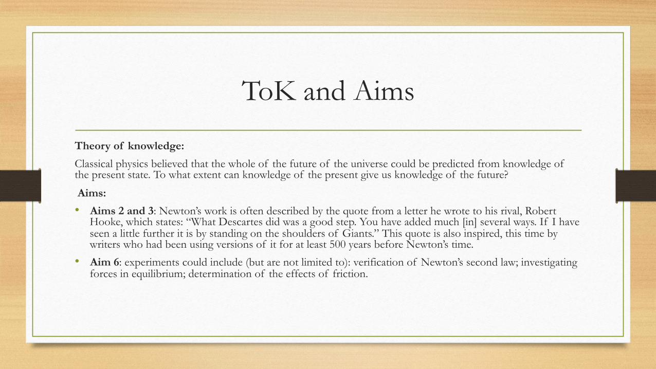
Theory of knowledge:
Classical physics believed that the whole of the future of the universe could be predicted from knowledge of the present state. To what extent can knowledge of the present give us knowledge of the future?
Aims:
• Aims 2 and 3: Newton’s work is often described by the quote from a letter he wrote to his rival, Robert Hooke, which states: “What Descartes did was a good step. You have added much [in] several ways. If I have seen a little further it is by standing on the shoulders of Giants.” This quote is also inspired, this time by writers who had been using versions of it for at least 500 years before Newton’s time.
• Aim 6: experiments could include (but are not limited to): verification of Newton’s second law; investigating forces in equilibrium; determination of the effects of friction.

Dynamics
Study of Force Essential idea: Classical physics requires a force to change
a state of motion, as suggested by Newton in his laws of motion.
Nature of science: (1) Using mathematics: Isaac Newton provided the basis for much of our understanding of forces and motion by formalizing the previous work of scientists through the application of mathematics by inventing calculus to assist with this. (2) Intuition: The tale of the falling apple describes simply one of the many flashes of intuition that went into the publication of Philosophiæ Naturalis Principia Mathematica in 1687.
Utilization: • Motion of charged particles in fields (see Physics sub-
topics 5.4, 6.1, 11.1, 12.2) • Simple Machines and Force multipliers • Application of friction in circular motion (see Physics
sub-topic 6.1) • Biomechanics (see Sports, exercise and health science SL
sub-topic 4.3) • Communications Satellites and the motion of planets

What is force?
Acceleration • As previously discussed, acceleration is the rate of change of
velocity.
• It is also then the second derivative of position/displacement (a rate of a rate).
• Acceleration is a vector quantity where the direction is reflected in the change in velocity.
Mass • Mass is the inertial property of matter.
• Massive objects resist change to their motions, which means it requires a greater force to accelerate them.
• You can observe this by attempting to move 2 objects, your pencil and the table. Moving one with your finger is easy, the other exceedingly difficult.
• Mass is a scalar quantity
Force: defined as a push or pull in a certain direction. Force is a vector quantity and results from the product of mass and acceleration (we’ll discuss this more later) F=ma. Then the units for force are kgm-2 which have been abbreviated by the synthetic unit Newton (N).
Common Forces: Gravity, Tension, Friction, Normal, and Centripetal We commonly refer to the force of gravity at the Earth’s surface as “weight” and has the very specific value of mg or the mass of the object times the acceleration due to gravity at the Earth’s surface 9.8 or 10ms-2. Tension: is the force distributed along a rope or rigid line. Tension in a line is the same anywhere on the rope and requires a counter force or anchor to bring the line to tautness, therefore tension is always a pull. Friction: is the force which opposes motion along a surface or through a fluid. This is one of the most common forces and always acts in the direction of –velocity, it is also parallel to the contact surface. Normal force: refers to the force perpendicular to the surface of contact between two objects. (Normal means perpendicular or at 90°)

Newton’s First Law
• Galileo was actually the first to suggest this. He observed that an object in motion will naturally remain in motion at a constant velocity until something outside of that object acted on it.
• You can simulate this with a steel ball on a hard surface or an air hockey table in either case, moving the object requires some input of force but once applied the object is free to move and will do so at constant velocity until some unbalanced force acts.
• Newton’s First Law: A body continues in its state of rest or uniform velocity as long as no net force acts on it. AKA Law of Inertia
• Inertial Reference Frames: classical mechanics are based upon the assumption that objects share a fixed reference frame on which no external forces are acting on the system. This is not always true:
• Ex: when you are in a car and the car accelerates you and the car share a reference and both accelerate in the same direction. The cup of scalding hot coffee you placed on the dash moments prior does not always share this and slides towards you. In this case you and the car share an inertial reference (you both have the same velocity at all times then the reference frame consisting of all things moving with shared velocity of the car are an inertial reference frame).

Newton’s Second Law
• If an object will move constantly when in motion then what will change that motion?
• When the velocity of an object changes, then it experiences an acceleration, when a mass accelerates it experiences a Net Force or a force which has not been offset by any other (remember, forces are vectors)
• How much acceleration an object experiences is directly proportional to the force applied (𝑭 α 𝒂 ). Forces are consequently also proportional to the mass of the object being accelerated ( 𝑭 α m ).
• These relationships lead Issac Newton to suppose that the acceleration of an object, for a given force, was inversely proportional to its mass 𝒂 α 𝟏/𝒎 .
• Newton’s 2nd Law: The acceleration of an object is directly proportional to the net force acting on it and is inversely proportional to its mass. The direction of the acceleration is equal to the direction of the net force. Newton’s second law is written as ∑↑▒𝐹 =𝑚𝑎

Newton’s Third Law
• Often we see interactions between more than one object. Generally, an object moves and experiences force because another object exerts a force on it. However, when one object interacts with the other, the first is never unchanged.
• Ex: a hammer hits a nail and drives it into a surface. The hammer exerts a force on the nail and pushes the nail into the substrate, but the hammer also comes to a stop.
• Newton’s Third Law: Whenever one object exerts a force on a second object, the second exerts an equal force in the opposite direction on the first.
• It can sometimes be confusing to work with such force pairs because you must keep track of the forces applied both by the first on the second and the second on the first when determining motion of the system.
• One way to keep things clear is by being careful to use subscripts to keep track:
• Ex: a person walking works by the person applying force to the ground. The person moves forward because the ground applies a force back on the person. Then the force applied on the ground by the person (𝐹 ↓𝐺𝑃 ) is equal to the force on the person by the ground (𝐹 ↓𝑃𝐺 ), but in the opposite direction. Then we can write this force pair as
• 𝐹 ↓𝐺𝑃 = -𝐹 ↓𝑃𝐺

Free Body Diagram
• In order to solve problems involving Newton’s 2nd law we need to have a way to determine which forces may or may not be in balance.
(remember 𝑭 net = ∑↑▒𝐹 =𝑚𝑎 ). • The best way to do this is by treating the object as a point mass (assuming all the mass is consisting of a single point) and therefore draw
the object as a small box or dot. Then we draw all the forces acting on that object as vector arrows with their origins at the point mass. This diagram of forces is called a Free Body Diagram (FBD)
• Ex: Determine all the forces acting on a box resting on a tabletop. Then draw a FBD for the book
• Ex: Draw the FBD for the book if it is being pulled horizontally to the right by a string across a table with friction. Now for a box pulled at a 30° angle with respect to the table
Fg = mg
Fg = mg
FN
FN FT
FF
Fg = mg
FN FT
FTx
FTy
FF
Θ

Applying Newton’s Laws • Ex: When we worked with ideal projectiles we noted that the
limiting factor for the flight of the projectile was the motion in y, use Newton’s 1st law to explain this.
• Ex: A book with mass 2.5kg rests on a tabletop. How much force must be applied to cause it to accelerate at 2ms-2? If it slides with a velocity after the push of 2ms-1 to a stop after traveling 0.75m, what is the force friction applies to the book to stop it?
• Ex: A 5kg box rests on a table. If a rope anchored to the box is pulled with a force of 25N; 20° what is the horizontal acceleration (assume no friction)? What is the normal force?
0.0
20.0
40.0
0.0 0.5 1.0 1.5 2.0
Dis
plac
emen
t (m
)
Time (s)
Object Motion in X
0.0
2.0
4.0
6.0
0.0 0.5 1.0 1.5 2.0
Dis
plac
emen
t (m
)
Time (s)
Object motion in Y
FApplied
xi = 0 xf = 0.75 vi = 2ms-1 vf = 0ms-1
Fg = mg
FN
FTx
FTy Θ
FBD

Problem with Tension and Connected Masses
• As previously mentioned tension is a force which is created when a force is applied to a flexible cord. If the cord has a negligible mass compared to the forces being applied to it (an assumption) then the force is transmitted unchanged throughout the length of the cord. This is because m ≈ 0 and F=ma is zero when m=0.
• Then the forces pulling on either end of the cord must sum to zero (FT and –FT )
Ex: For 2 masses connected by a cord with the rightmost mass being pulled by a force, Draw the FBD for BOTH masses
Given the information below, calculate the acceleration of each box and the tension in the cord connecting each box (assume the connecting cord remains taut and of fixed length).
Fg = m1g
FT FN M1 = 10kg
Fg = m2g
Fapplied = 60N
FT
FN M2 = 15kg
M2 = 15kg M1 = 10kg Fapplied = 60N
For M1
∑↑▒𝐹↓𝑥 = 𝑚↓1 𝑎↓𝑥 = 𝐹↓𝑎𝑝𝑝𝑙𝑖𝑒𝑑 − 𝐹↓𝑇 For M2
∑↑▒𝐹↓𝑥 = 𝑚↓2 𝑎↓𝑥 = 𝐹↓𝑇
For M1 and M2 FT = FT and ax is the same, then For M1
𝐹↓𝑇 = 𝐹↓𝑎𝑝𝑝𝑙𝑖𝑒𝑑 − 𝑚↓1 𝑎↓𝑥 For M2
𝐹↓𝑇 =𝑚↓2 𝑎↓𝑥
𝑚↓2 𝑎↓𝑥 =𝐹↓𝑎𝑝𝑝𝑙𝑖𝑒𝑑 − 𝑚↓1 𝑎↓𝑥
𝑚↓2 𝑎↓𝑥 +𝑚↓1 𝑎↓𝑥 =𝐹↓𝑎𝑝𝑝𝑙𝑖𝑒𝑑
𝑎↓𝑥 = 𝐹↓𝑎𝑝𝑝𝑙𝑖𝑒𝑑 /(𝑚↓1 + 𝑚↓2 ) = 60𝑁/(10𝑘𝑔+15𝑘𝑔) =𝟐.𝟒𝒎𝒔↑−𝟐
𝐹↓𝑇 =𝑚↓2 𝑎↓𝑥
𝐹↓𝑇 =15𝑘𝑔(2.4𝑚𝑠↑−2 )=𝟑𝟔𝑵

Elevator Problems (Atwood Machines)
When a mass is connected to another over a pulley a system of hanging masses is created whose gravitational forces offset. This is due to the ability of a cable to supply tension to both masses and the same direction. This principle is used to minimize the strength of a motor needed to operate an elevator system.
Ex: Consider an elevator (mE = 1150kg) and its counterweight (mC = 1000kg) suspended as shown in the diagram. If there is no motor and the brakes release in what direction will the elevator and counterweight move? Given what you know about systems of masses connected by a cable calculate a) acceleration of the elevator b) tension in the cable
For mE
∑↑▒𝐹↓𝑦 = 𝑚↓𝐸 𝑎↓𝑦 = 𝐹↓𝑇 − 𝑚↓𝐸 𝑔 −𝑚↓𝐸 𝑎↓𝑦 = 𝐹↓𝑇 − 𝑚↓𝐸 𝑔
𝐹↓𝑇 = −𝑚↓𝐸 𝑎↓𝑦 +𝑚↓𝐸 𝑔 For mC
∑↑▒𝐹↓𝑦 = 𝑚↓𝐶 𝑎↓𝑦 = 𝐹↓𝑇 − 𝑚↓𝐶 𝑔
𝑚↓𝐶 𝑎↓𝑦 = 𝐹↓𝑇 − 𝑚↓𝐶 𝑔
𝐹↓𝑇 = 𝑚↓𝐶 𝑎↓𝑦 +𝑚↓𝐶 𝑔
FT = FT
−𝑚↓𝐸 𝑎↓𝑦 +𝑚↓𝐸 𝑔= 𝑚↓𝐶 𝑎↓𝑦 +𝑚↓𝐶 𝑔
𝑚↓𝐸 𝑎↓𝑦 + 𝑚↓𝐶 𝑎↓𝑦 = 𝑚↓𝐸 𝑔-𝑚↓𝐶 𝑔
𝑎↓𝑦 = 𝑔(𝑚↓𝐸 − 𝑚↓𝐶 )/(𝑚↓𝐸 + 𝑚↓𝐶 ) = 𝑔(1150𝑘𝑔−1000𝑘𝑔)/(1150𝑘𝑔+1000𝑘𝑔) = 0.7ms-2
𝑎↓𝐸 = - 0.7ms-2
FT = 𝑚↓𝐶 𝑎↓𝑦 +𝑚↓𝐶 𝑔 FT = 1000kg (0.7ms-2 + 10ms-2) = 10.7(103)N

Tension as a Force Multiplier
• There is another method to utilize tension to multiply the amount of force you must input into a system compared to the force you can exert on an object. This method takes advantage of an anchor, pulleys, and the fact that tension is uniform along the length of a cable and has equal but opposite forces at the ends.
Block and Tackle By running a cable over a fixed pulley through a movable pulley (or multiple pulleys) you can create a system which uses a fixed anchor and tension to move far heavier loads than possible unassisted. Common set ups:
Ex: Gun tackle, using the provided diagrams, draw the free body diagram for the mass being lifted and calculate the mechanical advantage of this system. (note MA= mgT-1)
mg
FT1 FT2
FBD
∑↑▒𝐹↓𝑦 =𝑚𝑎↓𝑦 = 0=𝐹↓𝑇1 + 𝐹↓𝑇2 −𝑚𝑔 0= FT1 + FT2 –mg mg= FT1 + FT2 mg = 2FT
FT = 𝑚𝑔/2
MA = 𝑚𝑔/𝐹↓𝑇 = 𝑚𝑔/𝑚𝑔/2 = 2
Try yourself: Double tackle, use the same analysis as in the previous problem to determine the MA of this system. How much force would need to be applied to lift 1000kg?


Section 2.3: Work and Energy Conservation of Energy and the Energy of Motion/Position

Section 2.4: Momentum and Impulse
Changes in Energy in Time and Collisions

Section 4 Objectives
Core Principles
• Newton’s second law expressed in terms of rate of change of momentum
• Impulse and force – time graphs
• Conservation of linear momentum
• Elastic collisions, inelastic collisions and explosions
Applications and skills: • Applying conservation of momentum in simple isolated
systems including (but not limited to) collisions, explosions, or water jets
• Using Newton’s second law quantitatively and qualitatively in cases where mass is not constant
• Sketching and interpreting force – time graphs • Determining impulse in various contexts including (but not
limited to) car safety and sports • Qualitatively and quantitatively comparing situations
involving elastic collisions, inelastic collisions and explosions

ToK and Aims
Theory of knowledge:
Do conservation laws restrict or enable further development in physics?
Aims:
• Aim 3: conservation laws in science disciplines have played a major role in outlining the limits within which scientific theories are developed
• Aim 6: experiments could include (but are not limited to): analysis of collisions with respect to energy transfer; impulse investigations to determine velocity, force, time, or mass; determination of amount of transformed energy in inelastic collisions
• Aim 7: technology has allowed for more accurate and precise measurements of force and momentum, including video analysis of real-life collisions and modelling/simulations of molecular collisions

Momentum and Impulse
Study of Momentum • Students should be aware that F = ma is the equivalent of
F = Δp / Δt only when mass is constant
• Solving simultaneous equations involving conservation of momentum and energy in collisions will not be required
• Calculations relating to collisions and explosions will be restricted to one-dimensional situations
• A comparison between energy involved in inelastic collisions (in which kinetic energy is not conserved) and the conservation of (total) energy should be made
Utilization: • Jet engines and rockets • Particle theory and collisions (see Physics sub-topic 3.1) • Students should be aware that F = ma is the equivalent of F =
Δp / Δt only when mass is constant • Solving simultaneous equations involving conservation of
momentum and energy in collisions will not be required • Calculations relating to collisions and explosions will be restricted
to one-dimensional situations • A comparison between energy involved in inelastic collisions (in
which kinetic energy is not conserved) and the conservation of (total) energy should be made

Momentum • Linear momentum refers to the quantity described by the mass of an object multiplied by its velocity and is denoted with the symbol (p). Then the units for linear
momentum are kgms-1. As was the case for Force being a vector due to the product of a scalar and a vector, so too is momentum a vector.
• Momentum can be described in terms of Newton’s 2nd Law via the following derivation
• Remember that a = Δ𝑣/Δ𝑡 , and note that the delta refers to change from an initial value.
• If NII is ∑↑▒𝐹 =𝑚𝑎 then we can rewrite this as ∑↑▒𝐹 =𝑚Δ𝑣/Δ𝑡
• Then the sum of forces acting on an object equals the product of its mass and its change in velocity.
• p = m𝑣; then a change in momentum in time is Δp/Δ𝑡 = 𝑚𝑣↓𝑓 −𝑚𝑣↓𝑖 /Δ𝑡 ;
• If mass remains constant then we can rewrite this as Δp = 𝑚(𝑣↓𝑓 −𝑣↓𝑖 )/Δ𝑡 and remember that Δ𝑣 = (𝑣↓𝑓 −𝑣↓𝑖 )
• Then this becomes Δp/Δ𝑡 = mΔ𝑣/Δ𝑡 = ∑↑▒𝐹 or, written more familiarly as
• ∑↑▒𝐹 = Δp/Δ𝑡 the sum of forces acting on an object equals its change in momentum in time. In general, mass can change (such as is the case for rockets) and so when we use this equation in the general case we have to consider Δp = mfvf – mivi .
• Ex: What is the linear momentum of a 4.0-gram NATO SS 109 bullet traveling at 950 ms-1?
• Ex: A 6-kg object increases its speed from 5 m s-1 to 25 m s-1 in 30 s. What is the net force acting on it?
Data booklet reference: • p = mv • F = Δp / Δt • EK = p 2 / (2m) •Impulse = F Δt = Δp

Momentum and Kinetic Energy
• Given the relationship between force and momentum it should come as no surprise then that momentum and kinetic energy are related. We can write the kinetic energy equation in terms of momentum via the following rearrangement:
• If 𝑝=𝑚𝑣 and KE = 𝑚𝑣↑2 /2 then first let us solve the momentum equation for velocity
• 𝑣= 𝑝/𝑚 ; substitute this into the equation for kinetic energy and simplify
• KE = 𝑚[𝑝/𝑚 ]↑2 /2 = 𝑚𝑝↑2 /2𝑚↑2 ; • Then KE = 𝑝↑2 /2𝑚 (Now verify this equation using dimensional analysis)
• If KE can be written in terms of momentum and there is a conservation of energy law it should come as no surprise that there exists a law for the conservation of momentum in a system.
• This conservation of momentum is best explained by considering the momentum form of NII. If no external force acts on the objects in a system (that is,
moving objects with momentum interacting) then ∑↑▒𝐹 = Δp/Δ𝑡 = 0 or the total momentum is constant in time.
PRACTICE: What is the kinetic energy of a 4.0-gram NATO SS 109 bullet traveling at 950 m/s and having a momentum of 3.8 kg m s-1?
SOLUTION: You can work from scratch using EK = (1/2)mv
2 or you can use EK = p 2 / (2m).
•Let’s use the new formula…
EK = p 2 / (2m)
= 3.8 2 / (2×0.004)
= 1800 J.

Collisions and Momentum
• A collision is an event in which a relatively strong force acts on two or more bodies for a relatively short time.
Ex: The Meteor Crater in the state of Arizona was the first crater to be identified as an impact crater.
The object which hit was estimated to have released 3.8Megatons of energy. Assuming that all of the kinetic energy of the meteor was released, and the estimated velocity of the meteor is accurate (15km/s) estimate the mass of the meteor.
What then would have been the momentum of the meteor?
Given the extreme forces acting during the duration of this collision then how significant were the external forces of this impact? Is it safe to assume that momentum could be conserved during the collision?

Observing Collisions
• A collision between bodies has 3 distinct phases: Before, During, After. It is important to keep track of the momentum for EACH object during the collision in order to determine the forces and changes in momentum for the objects.
Before
p1i = m1vi1 p1i = m2v2
During
F1,2 = Δp1 F2,1 = Δp2
After
p1f = m1vf1 p2f = m2v2f
-30
-20
-10
0
10
20
30
0 0.2 0.4 0.6 0.8 1 1.2 1.4 1.6 1.8 2 Forc
e (N
)
Time (s)
Force Time Graph for 2 Body Collision Force1 Force2

Conservation of Momentum
• Collisions can be defined as closed systems, with system boundaries consisting of the objects involved in the collision only. This is useful as it allows us to derive a conservation law from the fact that the sum of external forces on the system is zero. This law is based on NII and NIII and can be derived in several ways.
• Let object A have momentum 𝒑 ↓𝑨 = 𝒎↓𝑨 𝒗 ↓𝑨 initially and object B have initial momentum 𝒑 ↓𝑩 = 𝒎↓𝑩 𝒗 ↓𝑩 • Then the total momentum of the closed system is the vector sum 𝑝 ↓𝑠𝑦𝑠𝑡𝑒𝑚 = 𝑝 ↓𝐴 +𝑝 ↓𝐵 = 𝑚↓𝐴 𝑣 ↓𝐴 +𝑚↓𝐵 𝑣
↓𝐵 • Following the collision each object has a momentum 𝑝 ↓𝑠𝑦𝑠𝑡𝑒𝑚↑ ′ = 𝑝 ↓𝐴↑ ↑′ + 𝑝 ↓𝐵↑′ =𝑚↓𝐴 𝑣 ↓𝐴↑′ +
𝑚↓𝐵 𝑣 ↓𝐵 ′ • Then the change in momentum Δ𝑝 ↓𝑠𝑦𝑠𝑡𝑒𝑚 = 𝑝 ↓𝑠𝑦𝑠𝑡𝑒𝑚↑′ − 𝑝 ↓𝑠𝑦𝑠𝑡𝑒𝑚 = (𝑚↓𝐴 𝑣 ↓𝐴↑′ +𝑚↓𝐵 𝑣 ↓𝐵
′) - (𝑚↓𝐴 𝑣 ↓𝐴 +𝑚↓𝐵 𝑣 ↓𝐵 ) • Now remember that ΣFsystem = Δ𝒑 ↓𝒔𝒚𝒔𝒕𝒆𝒎 /Δ𝒕 • But according to NII, ΣFsystem Δt = 0 = Δ𝒑 ↓𝒔𝒚𝒔𝒕𝒆𝒎 =𝒑 ↓𝒔𝒚𝒔𝒕𝒆𝒎↑′ − 𝒑 ↓𝒔𝒚𝒔𝒕𝒆𝒎 = ( 𝒎↓𝑨 𝒗 ↓𝑨↑′ +
𝒎↓𝑩 𝒗 ↓𝑩 ′) - ( 𝒎↓𝑨 𝒗 ↓𝑨 +𝒎↓𝑩 𝒗 ↓𝑩 ) • Then 𝑝 ↓𝑠𝑦𝑠𝑡𝑒𝑚 = 𝑝 ↓𝑠𝑦𝑠𝑡𝑒𝑚↑ ′ • And 𝒎↓𝑨 𝒗 ↓𝑨 +𝒎↓𝑩 𝒗 ↓𝑩 = 𝒎↓𝑨 𝒗 ↓𝑨 ′+𝒎↓𝑩 𝒗 ↓𝑩 ′ Conservation of Linear Momentum

Conservation Examples
• Ex: A 10,000kg railroad car A is traveling with a velocity of 24ms-1 to the east and strikes a car B whose mass is the same but is at rest. If the cars lock together then what is the common velocity of the cars afterwards?
pinitial = 𝑚↓𝐴 𝑣 ↓𝐴 + 𝑚↓𝐵 𝑣 ↓𝐵 = 𝑚↓𝐴 𝑣 ↓𝐴 pfinal = (mA + mB)v’ pinitial = pfinal
mAvA = (mA + mB)v’
v’ = mAvA/(mA + mB)
• Ex: calculate the velocity of recoil for a 5kg rifle firing a .020kg bullet with a speed of 620ms-1. Using this information then estimate the felt recoil (force) and compare shooting a rifle with a long barrel against shooting the same rifle but with a cut off barrel.
The system for a rifle and bullet consists of both objects having no momentum (v=0). Following the ignition of the primer the bullet is launched from the muzzle by a column of exploding gases. The bullet leaves moving in one direction but the rifle must then move in the opposite to conserve momentum.
pinitial = 𝑚↓𝑅 𝑣 ↓𝑅 + 𝑚↓𝐵 𝑣 ↓𝐵 = 0
pfinal = 𝑚↓𝑅 𝑣 ↓𝑅 ′+ 𝑚↓𝐵 𝑣 ↓𝐵↑′ pinitial= pfinal
0 = 𝑚↓𝑅 𝑣 ↓𝑅 ′+ 𝑚↓𝐵 𝑣 ↓𝐵↑′
𝑚↓𝐵 𝑣 ↓𝐵↑′ = −𝑚↓𝑅 𝑣 ↓𝑅 ′
𝑣 ↓𝑅 ′ = −𝑚↓𝐵 𝑣 ↓𝐵↑′ /𝑚↓𝑅
𝑣 ↓𝑅 ′ = −0.020𝑘𝑔∙620𝑚𝑠↑−1 /5𝑘𝑔 = -2.48ms-1
v’ = 10,000kg∙24ms−1/(20,000kg) =12ms-1
∑↑▒𝐹 = ∆𝑝/∆𝑡 What information might you need to assume? Then assume that the rifle recoil lasts about 0.3 seconds. F = 5kg·2.48ms-1 · 0.30s-1 ≈ 40N What about reducing the barrel? What does the butt pad do?

Impulse
• In the last example we discussed the effect of time over which a momentum changes as being related to force. Consider the force/time graph for the two objects during a collision:
-30
-20
-10
0
10
20
30
0 0.2 0.4 0.6 0.8 1 1.2 1.4 1.6 1.8 2 Forc
e (N
)
Time (s)
Force Time Graph for 2 Body Collision Force1 Force2
• We have shown previously that NII can be used to describe a change in momentum via , F ·Δt = Δp. Recall that this is similar to another situation (calculating displacement as Δx = v·Δt)
• Then likewise we can calculate the change in momentum by finding the area under a force time curve.
• Impulse : this is defined as the change in momentum calculated from F ·Δt. Impulse has the symbol J (not to be confused with the unit J for Joules in energy).
Ex: Estimate the impulse on object 1 during this collision. What do you notice about the impulse on 1 and 2?

More Practice for Impulse
• EXAMPLE: A 0.140-kg baseball comes in at 40.0 m/s, strikes the bat, and goes back out at 50.0 m/s. If the collision lasts 1.20 ms (this is a typical value):
• a) find the impulse imparted to the ball from the bat during the collision
• b) find the average force which acted on the ball during the collision with the bat
• c) estimate the impulse from the provided table of time and force values
a) SOLUTION: J = Δp = mv’ – mv = 0.140kg(50 - -40)ms-1 = 12.6kgms-1
b) SOLUTION:
J = Δp = ¯𝐹 Δt
12.6kgms-1 = ¯𝐹 ∙.0012s
¯𝐹 = 12.6𝑘𝑔𝑚𝑠↑−1 /0.0012𝑠 = 10,500N
Time (s) Force (N) 0 0
0.0002 0 0.0004 4 0.0006 27 0.0008 460 0.001 1500
0.0012 5300 0.0014 19,500 0.0016 6200 0.0018 3200 0.002 950
0.0022 45 0.0024 10 0.0026 0 0.0028 0 0.003 0
0 0 4 27 460 1500
5300
19,500
6200
3200
950 45 10 0 0 0 0
2000 4000 6000 8000
10000 12000 14000 16000 18000 20000
0 0.0002 0.0004 0.0006 0.0008 0.001 0.0012 0.0014 0.0016 0.0018 0.002 0.0022 0.0024 0.0026 0.0028 0.003
Forc
e (N
)
Time (s)
Force Time Curve of Baseball

Momentum and Rockets
• When a rocket is launched, fuel is burned rapidly which produces a steady supply of exhaust gases moving at very high velocity. Then the expelled gas has a tremendous momentum. In order for the momentum of the rocket body and gas system to be conserved, the rocket must also be given an equal and opposite momentum.
Draw the rocket/exhaust system including the FBD for the rocket. What is NII for this situation?
How does this system differ from previous examples in this unit?
Ex: a 25,000kg rocket burns fuel at a rate of 275kgs-1 and produces exhaust gases moving at 1250ms-1.
Determine the thrust of this rocket.
Bonus: At home determine the final velocity of the rocket if it holds 10,000kg of fuel when all the fuel is consumed (burnout). Show your work and include a description of the solution. +15points on momentum exam
Ex: How does a jet engine produce thrust?
Rocket exhaust
Air is pulled into the intake with a certain velocity and then heated and accelerated by the turbine fans. It is ejected at a much higher velocity which generates a powerful thrust due to the change in air momentum produces by the engine.

Elastic and Inelastic Collisions
• Elastic collisions defined as collisions in which all momentum is conserved and kinetic energy is conserved as well
• Then ma va + mb vb = mav’a + mbv’b and KEa +Keb = KE’a + KE’b