chapter 2 pulsed field gradients in high resolution...

Chapter 2 Pulsed field gradients in high resolution NMR

Chapter2

20

2.1 Pulsed field gradients in NMR The term pulsed field gradient is used for inhomogeneities of the static magnetic field

caused by the switching of dc-currents in coils surrounding the sample region in a

NMR spectrometer. The additional coils are usually designed such that the magnetic

field B0 they produce varies linearly over the sample region.

The use of pulsed field gradients had been suggested in 1963 in the context of

diffusion measurements (McCall, 1963). The influence of self-diffusion on the spin-

echo amplitude in the presence of a constant field gradient had already been discussed

by Hahn in his original paper on spin echoes (Hahn, 1950). The gradients were caused

by inhomogeneities of the static external field over the sample volume and the effect

of diffusion on the spin echo amplitude was disturbing the intended measurement of

spin-spin relaxation times. Separating relaxation from diffusion effects had been

achieved by a modified pulse sequence suggested by Carr and Purcell (Carr and

Purcell, 1954). This lead to a number of self-diffusion studies in viscous liquids (e.g.

(McCall, 1963)), but it was realized that the measurement of smaller and smaller

diffusion coefficients by constant field gradients became more and more unpractical.

The use of pulsed field gradients and stimulated echos led to a huge increase of the

sensitivity (Stejskal and Tanner, 1965). Frequency resolved spin-echo measurements

had been suggested by Vold et al. (Vold, 1968) soon after the introduction of the

Fourier transformation technique (Ernst and Anderson, 1966). An application to

measure self-diffusion coefficients of different components in complex systems using

pulsed field gradient Fourier transformation NMR followed (James and McDonald,

1973). This combination lead to wide spread applications in different parts of NMR

(Callaghan, 1991).

During a constant field gradient, the static magnetic field varies across the sample.

The Larmor frequency of a single resonance line is directly proportional to the

position within the sample. This effect can be used to obtain an image of the spin

density. This idea due to Lauterbur (Lauterbur, 1973) was the starting point of

spatially resolved magnetic resonance techniques with applications in biology,

medicine and material sciences (Blümich, 1998; Callaghan, 1991; Kimmich, 1997;

Miller, 1998; Vlaardingerbroek and denBoer, 1996).

Pulsed field gradients in high resolution NMR

21

The potential use of pulsed field gradients to perform signal selection in high-

resolution spectroscopy has been recognized in 1978 (Maudsley, 1978). Their routine

use in multi-dimensional NMR experiments was pioneered by Hurd (Hurd, 1990).

This development was triggered by the invention of actively shielded gradient coils. A

rigorous theoretical treatment of signal selection by pulsed field gradients was given

by Mitschang et al. (Mitschang, 1994; Mitschang, 1999). The finding of an optimal

sequence of pulsed field gradients for any NMR experiment has been reduced to a

geometrical problem. The development and application of a computer program based

on this theory is part of the underlying thesis. The results are discussed in (Thomas,

1999) as well as in paragraph 2.3.

Paragraph 2.2 gives an outline of the theory, which includes the discussion of coherent

motion and diffusion on the signal amplitude in a multi-pulse heteronuclear

experiment with pulsed field gradients. The geometric formulation of pathway

selection of Mitschang et al. is reproduced. The design of gradient pulse sequences is

discussed in detail in prepublished work (Thomas, 1999). Paragraph 2.3 gives

additional information on the treatment of pulse imperfections and optimizing water

suppression. Paragraph 2.4 discusses signal loss by diffusion.

2.2 Theory High-resolution multi-pulse heteronuclear experiments on liquid samples are most

conveniently discussed in terms of the product operator formalism (Ernst, 1987;

Sorensen, 1983). In the course of a NMR experiment, coherence is transferred

between nuclei, and superpositions of eigenstates of the spin system are excited.

These superpositions are conveniently classified into coherence orders p, standing for

the difference in the magnetic quantum numbers of the contributing eigenstates [for a

comprehensive discussion see for example (Levitt, 1988)]. The concept of coherence

order is particularly important in the description of experiments with pulsed field

gradients during free evolution intervals.

The Hamiltonian, which describes the interaction of a heteronuclear spin system with

a pulsed field gradient, is

Chapter2

22

( ) ( ) ( ) ( )

+−= ∑∑ )rrgGi

izSi

i

izIi StIttt γγH ( 2.1 )

where g = gradB(t) is the time dependent pulsed field gradient, ri the position of the

nuclear spin i, and Iz and Sz the Cartesian spin operators of species I (protons) and S

(heteronucleus) with the gyromagnetic ratios γI and γS. (For simplicity, only one

heteronuclear species is considered explicitly. If it becomes necessary, a

generalization of the equation to treat more than two different spin species can easily

be done.) The sum extends over all nuclear spins in the sample.

The Hamiltonian in this form contains the position of all spins as a function of time.

However, we are dealing with a liquid in a steady state of thermal motion. The motion

of the nuclear spins is a random process, and we have to introduce probability

concepts to describe the position of the spins. Brownian motion is a stochastic process

evolving in continuous time, and so we define a family of random variables Rt,

parameterized by the time t, and let rt denote the values taken by Rt (Gardiner, 1983).

The smallest length scale which can be sensed by pulsed field gradients is typically of

the order of µm (Callaghan, 1991). The size of the molecules in liquid NMR

experiments does not exceed a few nm. Therefore, the stochastic variables Rti are

taken to describe the motion of the center of mass of molecule i. Internal motions or

overall rotation of the molecule are neglected. In cases where the molecule gets

extremely big or the gradients very strong, additional internal variables have to be

included in the description.

The Hamiltonian then is

( ) ( )

+−= ∑∑ )(RgG

j

jzS

jzI

i

it SItt γγH ( 2.2 )

with the first sum extending over all molecules in the sample, and the second sum

including each spin of one molecule.

This Hamiltonian induces a spatially dependent precession of the spins in the

transverse plane. The precession frequency depends on the coherence order p and the

phase shift induced by a pulsed field gradient during a time interval r is given by


23

( ) it

rSS

rII t)pp( Rgγ+γ ( 2.3 )

with the coherence orders pIr and pS

r of the spins I and S present during the time

interval r. The different coherence orders excited during the experiment can be

collected in a coherence transfer pathway with an overall phase shift

( ) ( ) t d tt it

t

0

*i ′′=ϕ ∫ Rg ( 2.4 )

with the effective gradient g* being introduced to take care of the different coherence

orders during the experiment for simplicity purpose. The explicit form of the

dependence of the effective gradient on the coherence orders and gradient strengths

will be specified later. The detected signal of the NMR experiment is proportional to

the ensemble average

( ) ( ) ( ) ( )∑ ∫∫∑∈

ϕ ==i

it

*i0

i0

it

V

it

t

0iL

ti ti exp0,p0,|t,Pddte)(Si

t

i rgrrr rgr

* ( 2.5 )

with the conditional probability density

( ) ( )i0

i0

it

it

it

it

it

i0

it |dobPrd0,|t,P rRrrRrrrr =+<≤≡ ( 2.6 )

In the notation of (2.5), the stochastic process is defined by a family of random

variables Rti in continuous time. No further assumptions are made at this point about

the nature of the process. The ensemble average over the time integral of the phase

accumulated by a molecule i is defined by taking the ensemble average for each t,

where the Integral rti extends over all possible values that rt

i can take. This ensemble-

averaged quantity is then time integrated and the overall signal of the NMR

experiment is obtained by a summation of the contribution of each molecule.

The spatial average in (2.5) can be analyzed using the cumulant expansion theorem

(Stepisnik, 1981):

( ) ( ) ( )( )...tt

LiL +β−ϕϕ = ii iti ee ( 2.7 )

This corresponds to an expansion about the mean value

( ) ( ) t d ttL

it

t

0

*Li ′′ϕ ∫= Rg ( 2.8 )

Chapter2

24

The attenuation exponent βi is given by

( ) ( ) ( )∫ ∫ ′′′′′′=β ′′′

t

0

t

0

*

LC

it

it

*i tdtdtt

21t gRRg ( 2.9 )

In Eq. (2.9) the local correlation (Callaghan, 1991) or second order cumulant

L

itL

itL

it

itLC

it

it ′′′′′′′′′ −= RRRRRR ( 2.10 )

is introduced.

For a Gaussian phase distribution all cumulants of higher order than 2 vanish

(Gardiner, 1983). The local correlation is in that case equal to the variance σ of the

probability density. For a typical high resolution NMR setup the molecules inside the

sample diffuse freely, which means that the molecules do not hit any barrier during

the experiment. In this case the phases in (2.8) are Gaussian distributed and no higher

order corrections need to be applied. In cases of restricted diffusion in

microstructures, the Gaussian assumption or, as it is often termed in view of a

Stejskal-Tanner type diffusion experiment, the narrow-pulse criterion has to be

checked carefully (Wang, 1995).

The oscillatory part of the signal in (2.5) arises from the mean spin displacement. The

motion of the mean spin displacement can be expanded in powers of time (Callaghan,

1991)

( ) ( ) ( ) ( ) ...t dtt21t dttt dtt

t

0

*2t

0

*t

0

*Li +′′′+′′′+′′ϕ ∫∫∫= gagvgr ( 2.11 )

Where r is the average spin position in the sample measured from the origin of the

gradient coordinate system, v and a are the mean velocity and the mean acceleration.

This expansion presupposes that all spins in the sample have a common average

motion. In the case of a stagnant fluid only the first term of the expansion remains. If

the time integral over the effective gradient - hereafter referred to as the average

gradient - is vanishing, the signal phase does not depend on the position r of a

molecule. Therefore all molecules within the sample contribute with equal phase to

the signal. The signal is named "gradient echo" if the effective gradient is different

from zero during part of the time.


25

In cases where the average gradient is nonzero, the signal phase will encode for the

position of the spins within the sample. Recording a series of consecutive experiments

in which the average gradient is increased linearly from zero to a large value (or in

practice from a large negative to a large positive value) leads to a diffraction type of

signal modulation. The Fourier transform of the signal is a direct representation of the

projection of the spin density within the sample on the gradient direction. This linear

sampling of the signal decay in dependence of the average gradient is used extensively

in NMR imaging.

In high resolution NMR spectroscopy, the goal is to form a gradient echo for the

signal of interest. To evaluate the refocusing condition, the effective gradient has to be

specified explicitly. In a multi-pulse high resolution NMR experiment, the time

integral of Eq. (2.11) is decomposed into different intervals of free precession

separated by rf-pulses. During such an interval r, the coherence order is constant and

Eq. (2.4 )specifies the rate and sign of the gradient induced phase shift. The rf pulses

induce changes of coherence order. With the exception of 180° pulses, each pulse

changes the coherence order before the pulse into several new coherence orders after

it. These new coherence orders, which accumulated the same gradient induced phase

shift during the interval r, will collect different phase factors during the interval r+1

and have to be treated as separate terms. In this way, the rf-pulses create a multitude

of coherence order transfer pathways. Each of these pathways will be influenced in a

different manner by a sequence of pulsed field gradients. To evaluate Eq. (2.11), the

average gradient for one single coherence pathway can be written as

( )

( ) ( )

( ) ( )

( ) ( )

′′γ+γ

′′γ+γ

′′γ+γ

=′′

∫∑

∫∑

∫∑

∫δ+τ

τ=

δ+τ

τ=

δ+τ

τ=

t dtfGpp

t dtfGpp

t dtfGpp

t dt

rr

r

rr

r

rr

r

rz

rz

F

1r

rSS

rII

ry

ry

F

1r

rSS

rII

rx

rx

F

1r

rSS

rII

t

0

*

g ( 2.12 )

The time integral is expressed as sum over all free evolution periods of the

experiment. Pulsed field gradients are applied at times ττττr with amplitudes

Gααααr (α=x,y,z) and shape factors fαααα

r in the interval r of the experiment during which

the coherence orders pIr and pS

r are excited. The shape factor fαr is a smooth function

Chapter2

26

with a maximum value of 1, which is non-zero only during the time interval [τr, τr+δr].

F is the total number of free evolution intervals of the experiment. By further

introducing the composite coherence order p (John, 1991; Mitschang, 1994) and the

gradient strength sαr

rS

S

IrI

r ppp

γγ+= ( 2.13 )

( ) t dtfGsrr

r

rrr ′′= ∫δ+τ

τααα ( 2.14 )

the condition for a vanishing average gradient reads

( ) 0

1

1

1

0

kpspsps

g

z

y

x

=−=

=

=′′

∑

∑

∑

∫

=

=

=

I

F

r

rz

r

F

r

ry

r

F

r

rx

r

I

t*

sp

sp

sp

t dt γγ ( 2.15 )

with the gradient strengths along the Cartesian axes sα (α=x,y,z) and the composite

coherence orders p written as a vector with F components. Eq. (2.15) defines the

general wave vector k.

The resulting signal amplitude from the oscillating part in (2.5)

( ) ( ) ( )Lk

LksinRk

RkJ2S

S

z

z

r

r1

0

=kr ( 2.16 )

where the sample volume is taken to be a cylinder of height L and radius R with

uniform spin density. Its center is the origin of the coordinate system and its axis of

cylindrical symmetry along the Zeeman field. The radial component of the wavevector

is kr =(kx2+ ky

2)½ (Mitschang, 1999; Thomas, 1999).

Eqs. (2.16) and (2.15) reduces the finding of an optimal gradient sequence for a given

pulse sequence to a geometrical problem (Mitschang, 1994). The condition (2.15) has

to be fulfilled for all selected coherence transfer pathways simultaneously, while the

factor (2.16) should be as small as possible for all pathways to be suppressed. The

solution of this multidimensional minimization problem is found with the aid of the


27

computer programs Z GRADIENT and TRIPLE GRADIENT and is discussed in more

detail in section 2.3.2.

The second term in the expansion of Eq. (2.7) leads to a damping of the signal for all

coherence pathways. This damping is caused by the statistical fluctuations of the

average molecular motion. The location correlation in its general form of Eq. (2.10) is

a second rank tensor.

The diffusion coefficient of a particle undergoing Brownian motion can be defined in

two different ways. (1) In the phenomenological approach, a concentration gradient

causes a particle current density j proportional to the concentration gradient grad c.

The constant of proportionality is called the diffusion constant D (Fick's law). (2) The

second approach is a microscopic approach. Here the self-diffusion tensor is defined

as the spectral density function of the particle velocity auto-correlation:

( ) ∫∞

∞−

ωβαβα =ω dteVV

21D ti

L

it

it, ( 2.17 )

In the limit of zero frequency, the two definitions are equivalent for non-interacting

Brownian particles (Ohtsuki and Okano, 1982). The relationship between the particle

velocity auto-correlation and the local correlation is described in detail in (Callaghan,

1991). The result is

( )( )

z y,x, 12 ==

′′−′∞

∞−′′′ ∫ αω

ωω

παα

ω

αα deDtti

LC

it

it ( 2.18 )

In this case (2.9) might be expressed as (Stepisnik, 1981; Stepisnik, 1985)

( ) ( ) ( ) ωωω

ωπ

=β α=α

∞

∞−

αα∑ ∫ dt,g~D21t

2*

z,y,x2i ( 2.19 )

where the Fourier transform of the effective gradient

( ) tdegt,g~t

0

ti** ′=ω ∫ ′ωαα ( 2.20 )

has been introduced.

Chapter2

28

The attenuation factor in Eq. (2.19) depends on the spectral density of the translational

motion and the squared spectrum of the effective gradient. The analogy between this

expression and equations for spin relaxation has been pointed out by Callaghan

(Callaghan, 1991; Callaghan and Stepisnik, 1995). In relaxation, the spectral density

of the random rotational motion of the molecule is sampled at frequencies

corresponding to the Larmor frequencies of the involved spins, their sum and

difference. In a diffusion experiment the spectral density of the random translational

motion is sampled with the function

( ) ( )2

2* t,g~t,S

ω

ω=ω α

α ( 2.21 )

which is characteristic of the gradient spectrum. However, in terms of this analogy, we

maneuver in the regime of extreme motional narrowing for aqueous protein solutions,

e.g. the function Dαα(ω) can be replaced by Dαα(0), which represents the self-diffusion

coefficient along the Cartesian axis α. If a model of Brownian motion is assumed, the

characteristic time scale for the motion will be the jump time of the random walk

(Callaghan, 1991)

( )0D

V2i

t

Cαα

α

≈τ ( 2.22 )

which is of the order of pico-seconds for simple liquids. In contrast the fastest time

scale of the gradient variation is typically not faster than a few µs, which is several

orders of magnitude larger. Thus it is impossible to study spectral features of the

translational motion in simple liquids or protein solutions.

The Parceval relation

( ) ( ) dutdtgdt,g~

21 t

0

2u

0

*2

2*

∫ ∫∫ ′′≡ωωω

π α

∞

∞−

α ( 2.23 )

in combination with Eqs. (2.5), (2.7) and (2.19), with D(ω) being replaced by D(0),

gives two different general expressions of the signal attenuation due to diffusion. In

the frequency domain, we get


29

( )( )

( )

ωωω

π−=

= ∑ ∫=α

∞

∞−

ααα d

t,g~D

21exp

0S,S

z,y,x2

2*

s

p s ( 2.24 )

and in the time domain, we get

( )( ) ( )

′′−== ∑ ∫ ∫

=αααα

z,y,x

t

0

2u

0

* dutdtgDexp0S

,S s

p s ( 2.25 )

Eqs. (2.24) and (2.25) describe the attenuation factor of one single coherence transfer

pathway with the coherence orders represented by the vector p (see (2.13)) in an

experiment with pulsed field gradients, the strength of which is represented by the

vector s (see (2.14)). On the right hand side the explicit dependency on p and s is

hidden in the effective gradient g*. A general solution of this equation with an explicit

representation of the effective gradient in terms of p and s and its implication to

protein experiments will be discussed in paragraph 2.4. In case of a non-vanishing

average gradient (2.12), the diffusion factor (2.24) or (2.25) has to be multiplied with

the position dependent factor (2.16) to get the total attenuation due to the pulsed field

gradients.

The result given in Eq. (2.25) reproduces earlier results (Kenkre, 1997; Stejskal and

Tanner, 1965) which had been obtained by solving the classical Bloch-Torrey

equations (Torrey, 1956).

2.3 Pathway selection and artifact suppression

2.3.1 General remarks The selection of coherence transfer pathways is essential to any multi-pulse sequence.

Depending on the coherence selection, the spectra obtained of an otherwise identical

sequence of pulses can differ immensely. Selection of coherence transfer pathways

can be done by phase cycling (Bain, 1984; Bodenhausen, 1984; Kessler, 1988). The

pulse sequence, especially with the same time increment in a multidimensional

experiment, is repeated a certain number of times only changing the phases of one or

more of the pulses and the receiver. The signals of all scans are then added up in the

receiver, where the wanted pathways accumulate, whereas the unwanted ones are

cancelled by subtraction. This selection principle causes some problems:

Chapter2

30

1. Small changes in amplitude or phase between the scan lead to incomplete subtraction, causing so called t1-noise. Traces of noise appear as lines along the indirect dimensions at the detection frequency of large suppressed signals.

2. The FID acquired in a single scan contains all possible pathways of the experiment, which have to be fully digitized in the receiver. The choice of the receiver gain is often determined by large unwanted signals and small wanted signals are not digitized properly (dynamic range).

3. The measurement time can get exceedingly long, depending on the required number of scans to complete a phase cycle. This is especially inconvenient for concentrated samples, where one scan per time increment could often give a satisfying signal to noise ratio.

An alternative to the phase cycling is the pathway selection by pulsed field gradients.

Whereas the selection via phase cycling is based on the change of coherence order, the

effect of a pulsed field gradient is sensitive to the coherence order itself (2.3). The

condition for refocusing a pathway is given in Eq. (2.15). It can be analyzed in a

straightforward manner to get a gradient sequence that does not suppress any of the

wanted pathways. However, it should be noted, that the refocusing of one or more

wanted pathways is not sufficient for a selection. In order to perform a real selection,

it must be made sure that all possible unwanted pathways are dephased at the same

time by the gradient sequence. The finding of such a sequence is by no means trivial.

The main advantage of the use of pulsed field gradients is the fact that the selection

procedure is done in one scan, which circumvents the problems of phase cycling

mentioned above. On the other hand, there are major disadvantages of using pulsed

field gradients as well:

1. The application of a pulsed field gradient induces eddy currents in any conductor near the coil.

2. A mechanical torque is applied to the gradient coil and thus to the probe. Both effects 1 and 2 disturb the stability of measurements.

3. The application of pulsed field gradients takes some extra time in many cases. This leads to loss of magnetization due to relaxation. Loss of magnetization due to diffusion is unavoidable as well.

4. If the wanted pathways are dephased before an amplitude type of magnetization transfer occurs during the experiment, half of the wanted pathways are lost and the signal intensity is reduced by a factor of 2 or 2½ (Mitschang, 1999).

Although the potential of the use of pulsed field gradients had been recognized very

early on (Maudsley, 1978), the first point listed above has prevented the application in

spectroscopy for a long time. The induced eddy currents can last long enough to

inhibit the recording of a high-resolution spectrum for several hundred milliseconds


31

after the application of a pulsed field gradient. Thanks to the invention of actively

shielded gradient coils (Mansfield and Chapman, 1986; Mansfield and Chapman,

1987; Turner and Bowley, 1986), the routine use of pulsed field gradients in

spectroscopy was made possible. In their design, an additional shield coil is wound

around the main gradient coil to compensate the field outside the sample volume. For

such a coil design, eddy currents decay in times of the order of a hundred

microseconds.

The problem of the mechanical disturbance is not so severe since the gradient

strengths required for signal suppression are not very high. A typical problem induced

by this force are vibrations of the sample, which might cause traces of t1 noise at a

frequency of a few ten to hundred Hertz next to strong signals. Fixing the gradient coil

tightly to the probe solves the problem.

The signal decay due to diffusion - which will be discussed in more detail in section

2.4 - is more of a problem for small molecules, which have long transverse relaxation

times. For this class of molecules, some extra delay of one to three milliseconds does

not affect the signal intensity very much. For large molecules though, the relaxation

losses during such an interval might be intolerable. On the other hand the signal loss

by diffusion can be neglected for large molecules.

The relaxation problem exists only for pulse sequences, which require a gradient

during a delay that encodes the chemical shift in an indirect dimension. In those cases,

the extra chemical shift evolution during the pulsed field gradient has to be refocused

by a 180° Pulse. An alternative is to calculate the first points of the FID by linear

prediction (Ross, 1993). This induces some artifacts of the lineshapes, if too many

points have to be predicted.

The most severe problem in biological applications, where the signal to noise ratio of

an experiment is crucial, is the signal reduction mentioned in point 4 above. Most

multidimensional heteronuclear NMR experiments involve the transfer of

magnetization via J-coupling evolution. Magnetization evolves from transverse in-

phase magnetization Ix or Iy into antiphase magnetization IySz or IxSz. The

magnetization transfer is accomplished by a simultaneous 90° pulse on the I and S

spins, which gives a rotation for the full antiphase magnetization that did build up

Chapter2

32

during the previous delay. Now the rest of the pulse sequence is designed to “work”

only on the magnetization that has been rotated. Placing a pulsed field gradient into

that interval will spread e.g. the IySz part into equally distributed IySz and IxSz, so that

the following Ix pulse only rotates half of the initial antiphase magnetization, and

since the pulse sequence is designed to continue working only on IzSy, the other half

of the magnetization is lost (Muhandiram, 1994). The problem is circumvented, if the

pulse sequence does continue working on both parts of the resulting magnetization as

for example in a homonuclear isotropic TOCSY transfer. Thus gradients might be

applied in these sequences without losing sensitivity (Sattler, 1995; Wijmenga, 1997).

The situation is different if a gradient is placed into an indirect evolution period. The

magnetization precesses in the x-y plane while the indirect time domain is

incremented and a subsequent 90° pulse flips only half of the magnetization on

average. The resulting signal is amplitude modulated, which implies that the sign of

the rotation during t1 is lost. To ensure that no scrambling occurs, the reference

frequency has in principle to be placed to one side of the spectral region (Aue, 1976).

However, methods have been developed, that circumvent this problem by shifting the

phase of the pulses before the acquisition period (Marion, 1983; States, 1982). In this

method the reference frequency can be placed in the center of the spectrum and an

improvement by a factor 2½ in signal to noise ratio is reached by avoiding the folding

of noise into the spectral region by the reduced spectral window. If gradients are

placed in the indirect time domain, again half of the magnetization is flipped as in the

phase-cycled version. The frequency in the indirect dimension can easily be

determined, however the peaks have unfavorable mixed line shapes. To circumvent

this problem, two transients selecting p- and n-type coherence have to be added. This

leads to the same type of amplitude modulated signal as in the States method, but the

2½ intensity gain is lost (Keeler, 1985, Muhandiram, 1994 #38).

A way to work around the 2½ is by using a so-called sensitivity enhanced experiment

(Cavanagh, 1991; Palmer III, 1991; Palmer III, 1992). In the indirect chemical shift

dimension, the phase e.g. of the 2IzSy magnetization has a cos(Ωt1) dependency, and

so a 90° pulse at the end of the interval t1 flips the Sy magnetization only half the time.

In total one gets an average over the cosine term, which leads to a factor 2½ loss of

signal to noise that is unavoidable for all indirect dimensions that evolve chemical


33

shifts. The 2IySz term created after t1 evolves into inphase proton magnetization Ix in

an INEPT step and is detected subsequently, whereas the 2IySx term is lost. The trick

in sensitivity enhanced experiments is now to “park” the inphase term Ix created by

the INEPT along the z-axis. At the same time the double/zero quantum term 2IySx is

converted to antiphase 2IySz which in turn evolves into inphase Ix in a second INEPT

step. Afterwards the parked Iz term is flipped to the transverse plane by a x-pulse. As a

result, the total transverse magnetization present in t1 will be transferred from spins S

to I (for a two spin-system IS). In a sense heteronuclear primary and stimulated echoes

(Hahn, 1950) are recorded at the same time with a 90° phase difference, and

unsurprisingly there is no loss in sensitivity when gradients are employed (Kay, 1992).

Another way to fully refocus the magnetization would be the application of a rf-

gradient. The method of spectral editing with rf-gradients has been long recognized

(Counsell, 1985). The B1 inhomogeneity of the rf coil can be used to dephase

magnetization. This method has been applied for example the suppression of zero-

quantum coherences in NOESY spectra, which is not possible by pulsed field

gradients or phase cycling (Mitschang, 1992). The desired magnetization is spin-

locked by the rf-pulse and any component perpendicular decays.

As is the case for static pulsed field gradients, the decaying signal can be refocused by

applying a gradient with opposite polarity. In such a case the phase of the signal does

not depend on the position of the spins and a so-called rotary spin echo forms

(Solomon, 1959). The greatest inhomogeneities of the rf field exist outside a standard

coil used for high resolution NMR, where the magnetization decays approximately

proportional to the inverse of the coil radius. This rf-gradient could lead to partial

refocusing of prior static pulsed field gradients in z-direction (Czisch, 1996). On the

other hand, static pulsed field gradients might be used to suppress B1 inhomogeneities

(Hurd, 1992). These applications all use the natural inhomogeneity of the standard

coil of the spectrometer, which is not at all designed to be inhomogeneous. Another

approach is to design probes, which contain an additional coil producing a linear rf-

gradient (for a review see (Canet, 1997)). This rf-gradient can be used in much the

same way as a static pulsed field gradient for coherence selection (Brondeau, 1992;

Maas, 1993; Mutzenhardt, 1995), imaging (Hoult, 1979; Maffei, 1994; Metz, 1994) or

diffusion experiments (Canet, 1997; Humbert, 1998; Kimmich, 1995; Simon, 1996).

Chapter2

34

The important point to note is that the dephasing by the rf-gradients occurs in a plane

perpendicular to the effective field, e.g. the x-z plane, while static pulsed field

gradients dephase in the x-y plane. In a sequence, static pulsed field gradient - (90°)x-

(rf-gradient)y, all magnetization should be refocused, if both gradients show the same

positional dependence and have the same strength. Maximum sensitivity can be

obtained with the combined B0 B1 gradient selection. The problem remains to design a

probe with linear B0 and B1 gradients.

An amazingly simple way of achieving selection is to store the desired magnetization

along the z-axis and apply a pulsed field gradient that purges all unwanted signals,

which remained in the transverse plane. Because this method does not imply any

dephasing and rephasing of the desired pathways, it is sometimes not viewed, as a

“real” coherence selection by gradients, but the distinction is rather superficial. If all

possible unwanted pathways are purged by a gradient, the gradient does indeed do the

selection job. Examples are the application of a pulsed field gradient in the NOESY

mixing time or gradients in so-called z or zz filters (Bax, 1992; John, 1992). A zz-

filter can be introduced at the end of any INEPT or the beginning of a back INEPT

step in a heteronuclear pulse sequence. Additional z-filters might be introduced before

acquisition (Wider and Wüthrich, 1993).

In the discussion so far, all rf-pulses of the experiment have been assumed to be ideal,

e.g. the desired rotation angle is expected to be the same over the whole sample

volume and the whole frequency range. This is never the case in real experiments

though; there will always be a number of artifacts caused by pulse imperfections.

Particularly 180° pulses are sources of artifacts in spectra. An easy way to remove a

bigger proportion of the imperfections of these pulses is to flank them by two pulsed

field gradients of the same magnitude (Bax, 1992), a procedure which is very familiar

in imaging applications, where pulse imperfections of 180° pulses are far more severe.

The main advantage of pulsed field gradients in biological applications is the very

efficient water suppression. The water signal in protein samples of concentrations of

1mM or less in pure water can be reduced to be smaller than a typical signal from the

protein. There are a large number of publications on this topic and the reader is

referred to reviews (Aliteri, 1996; Hore, 1989). The only special water suppression

technique to be mentioned here is the so-called WATER GATE. It is based on a Hahn


35

echo sequence with a selective pulse for the water magnetization (Liu, 1998; Piotto,

1992; Sklenar, 1993). The pulses are flanked by two identical pulsed field gradients,

which refocus the desired signal and dephase the water magnetization.

2.3.2 The Design of Gradient Pulse Sequences The general condition for the formation of a heteronuclear gradient echo has been

developed in section 2.2:

The following paragraph is taken from (Thomas, 1999) which discusses the

development of a computer program, based on the geometrical analysis. In the

example given in (Thomas, 1999), we discuss an experiment, which produces several

types of high order coherence. The experiment selects heteronuclear quadruple

quantum coherence, while heteronuclear triple and double quantum coherence are

suppressed.

The attenuation of a pathway depends on the vector argument, k, which appears as the scalar component kr and kz in equation (2.16). k itself depends on the inner product of the vectors p and s, which is what makes it possible to interpret the mechanism of pathway selection geometrically. A pathway is rephased if k=0 when field gradients are applied. In this case, the vectors sx, sy and sz representing the sequences of pulsed filed gradients applied along the different directions are orthogonal to the vector p representing the coherence transfer pathway. For k different from zero, i.e. if one of the vectors sx, sy and sz are not orthogonal to p, the pathway is dephased and hence attenuated to a certain extent. Generally speaking, the larger the inner product between the pathway and the sequences of field gradients, the greater is the achievable attenuation of the signal because of the way in which Eq. (2.16) falls off.

The overall vector space RF splits naturally into three parts. The first is the subspace spanned by the wanted pathways, and is hence called ‘selective’. The remaining part of RF is decomposed into two further parts. The suppressive subspace comprises the components of the unwanted pathways outside of the selective subspace, whilst the free subspace is any remaining part of RF that can be spanned neither by wanted nor by unwanted pathways.

The condition that a gradient sequence not perturbs the wanted signals can now be met simply by generating it from within the suppressive and free subspaces, and avoiding the selective one. The suppression of unwanted pathways depends entirely on components from the suppressive subspace. (Thomas, 1999)

In most of the pulse sequences in use for protein structure determination (Kay, 1995a;

Kay, 1995b; Sattler, 1999) the situation is quite different. No higher coherence orders

are excited and the number of possibilities of introducing gradients for coherence

Chapter2

36

order selection without reducing the signal to noise ratio of the experiment is very

limited (Muhandiram, 1994). Usually the last back INEPT is replaced by the

sensitivity-enhanced version. The two gradients inserted provide very good water-

suppression and do the coherence selection (for 2 dimensions). Apart from these two

gradients, a different number of additional gradients are placed around 180° Pulses

and in zz-intervals (Bax, 1992). These gradients serve to suppress artifacts and

prevent radiation damping of the water, in the case where water flip-back sequences

are employed (Kay, 1994). The experiment is viewed as consisting of simple building

blocks. The possible artifacts during such a building block are suppressed by applying

pulsed field gradients in the way mentioned above. The ratio of the gradient strengths

applied in different building blocks is optimized empirically, where the most crucial

factor is the efficiency of the obtained water suppression. The gradient strengths are

varied in non-integer ratios to avoid accidental refocusing of unwanted signals. The

following discussion will show a way how this empirical procedure can be replaced

by a systematic approach.

The approach is discussed on the example of the HSQC sequence with a

WATERGATE (Fig. 2.1) and two zz-intervals. This relative simple pulse sequence is

chosen, because the number of unwanted pathways identified by the formalism

outlined below is small enough to be listed and discussed in detail within this thesis.

The sensitivity enhanced version of the HSQC sequence or any other

multidimensional experiment can be treated in a similar way, but the number of

unwanted pathways increases relatively quickly if more free precession intervals are

added.


37

1H

15N

∆ δt1/2t1/2

GARP

∆

1 2 3 4 5 6 7 8

δ

Gx-15.7 0.38 -12.6 -12.6

Gy

13.3

-10.4 -9.5 -9.5

Gz -19.8

12.9

5.0 5.0

y

x-x

x-x-x

Fig. 2.1 HSQC with 3-9-19 WATERGATE and two zz-intervals. ∆∆∆∆=1/2JHN or slightly shorter and δδδδ=(2∆∆∆∆-3.37t)/2 to compensate for JHN evolution during the (3)x-ττττ-(9)x-ττττ-(19)x-ττττ-(19)-x-ττττ-(9)-x-ττττ-(3)-x pulse-train. The first increment in the indirect dimension is calculated to be (t1)0=n/(2*SW)-[(4/ππππ)*tππππ/2(15N)+tππππ(1H)] to calculate the phase correction in F1 or back-predict the point t1=0 (Schmieder, 1991) (n=0,1,2,.. , SW=spectral width in the 15N dimension, tππππ/2(15N)=90° Pulse length of nitrogen, tππππ(1H)=180° Pulse length of the protons). Phase cycling: φφφφ1=x,-x,x,-x; φφφφ2=x,x,-x,-x; rec=x,-x,-x,x. Optimized gradient values are shown in lines Gx, Gy and Gz (see text).

Chapter2

38

In the HSQC experiment, the equilibrium magnetization Iz is rotated by the first 90°

pulse on the protons to the transverse plane. During the first INEPT (intervals 1 and 2)

antiphase proton magnetization IySz builds up, which is turned into spin order IzSz.

The first 90° pulse on 15N excites antiphase nitrogen magnetization IzSy that evolves 15N chemical shift during t1. The 180° pulse on the protons in the middle of t1

refocuses the heteronuclear coupling. At the end of t1, the magnetization is again

stored as IzSz and finally transferred back to inphase proton magnetization, which is

subsequently detected while the heteronucleus is decoupled. The pulse sequence has 8

periods of free precession in which pulsed field gradients can be placed. The

coherence order of all desired pathways during these intervals are shown in Tab. 2.1.

number 1 2 3 4 5 6 7 8 1 +1 -1 0 +0.1 +0.1 0 -1 -1 2 +1 -1 0 -0.1 -0.1 0 -1 -1 3 -1 +1 0 +0.1 +0.1 0 -1 -1 4 -1 +1 0 -0.1 -0.1 0 -1 -1

Tab. 2.1 List of the four wanted coherence transfer pathways in the 1H15N HSQC experiment. The numbers in the first row refer to the intervals of free precession as shown in Fig. 2.1.

For the HSQC the origin of artifacts has been described in detail in the literature

(Cavanagh, 1996; Hammarström, 1994; Shaw, 1996). Imperfections in 180° pulses

including off-resonance effects and non-ideal flip angle due to rf-inhomogeneities or

wrongly determined pulse-lengths are the cause of all artifacts. All of these artifacts

can be analyzed in detail by a full product operator treatment. Choosing this approach

gives exact results, but it requires a substantial amount of computation, especially if

the pulse sequence under consideration is getting more complicated. For an efficient

suppression of the resulting artifact, it should generally be enough to get an estimate

of the effect of the imperfections. The effect of a pulse with flip angle Φ along the x-

axis can be expressed as (Ernst, 1987)

( ) Φ−−Φ → −+Φ sinIIi2

1cosII zI

zx ( 2.26 )

Φ±Φ+Φ → ±Φ± siniI2

sinI2

cosII z22Ix µ ( 2.27 )


39

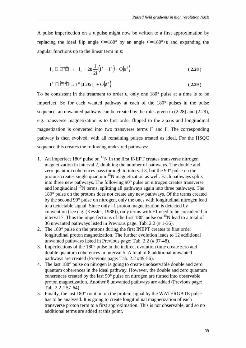
A pulse imperfection on a π pulse might now be written to a first approximation by

replacing the ideal flip angle Φ=180° by an angle Φ=180°+ε and expanding the

angular functions up to the linear term in ε:

( ) ( ) ( )2z

Iz OII

i212II x ε+−ε+− → −+ε+π ( 2.28 )

( ) ( )2z

I OiI2II x ε+ε → ε+π± µµ ( 2.29 )

To be consistent in the treatment to order ε, only one 180° pulse at a time is to be

imperfect. So for each wanted pathway at each of the 180° pulses in the pulse

sequence, an unwanted pathway can be created by the rules given in (2.28) and (2.29),

e.g. transverse magnetization is to first order flipped to the z-axis and longitudinal

magnetization is converted into two transverse terms I+ and I-. The corresponding

pathway is then evolved, with all remaining pulses treated as ideal. For the HSQC

sequence this creates the following undesired pathways:

1. An imperfect 180° pulse on 15N in the first INEPT creates transverse nitrogen magnetization in interval 2, doubling the number of pathways. The double and zero quantum coherences pass through to interval 3, but the 90° pulse on the protons creates single quantum 15N magnetization as well. Each pathways splits into three new pathways. The following 90° pulse on nitrogen creates transverse and longitudinal 15N terms, splitting all pathways again into three pathways. The 180° pulse on the protons does not create any new pathways. Of the terms created by the second 90° pulse on nitrogen, only the ones with longitudinal nitrogen lead to a detectable signal. Since only –1 proton magnetization is detected by convention (see e.g. (Kessler, 1988)), only terms with +1 need to be considered in interval 7. Thus the imperfections of the first 180° pulse on 15N lead to a total of 36 unwanted pathways listed in Previous page: Tab. 2.2 (# 1-36).

2. The 180° pulse on the protons during the first INEPT creates to first order longitudinal proton magnetization. The further evolution leads to 12 additional unwanted pathways listed in Previous page: Tab. 2.2 (# 37-48).

3. Imperfections of the 180° pulse in the indirect evolution time create zero and double quantum coherences in interval 5. A total of 8 additional unwanted pathways are created (Previous page: Tab. 2.2 #49-56).

4. The last 180° pulse on nitrogen is going to create unobservable double and zero quantum coherences in the ideal pathway. However, the double and zero quantum coherences created by the last 90° pulse on nitrogen are turned into observable proton magnetization. Another 8 unwanted pathways are added (Previous page: Tab. 2.2 # 57-64)

5. Finally, the last 180° rotation on the protein signal by the WATERGATE pulse has to be analyzed. It is going to create longitudinal magnetization of each transverse proton term to a first approximation. This is not observable, and so no additional terms are added at this point.

Chapter2

40

1 2 3 4 5 6 7 8 1 +1 -0.9 +1.1 +1.1 -0.9 -1 +1 -1 2 +1 -0.9 +1.1 +1 -1 -1 +1 -1 3 +1 -0.9 +1.1 +0.9 -1.1 -1 +1 -1 4 +1 -0.9 +0.1 +0.1 0.1 0 +1 -1 5 +1 -0.9 +0.1 0 0 0 +1 -1 6 +1 -0.9 +0.1 -0.1 -0.1 0 +1 -1 7 +1 -0.9 -0.9 -0.9 +1.1 +1 +1 -1 8 +1 -0.9 -0.9 -1 +1 +1 +1 -1 9 +1 -0.9 -0.9 -1.1 +0.9 +1 +1 -1

10 +1 -1.1 +0.9 +1.1 -0.9 -1 +1 -1 11 +1 -1.1 +0.9 +1 -1 -1 +1 -1 12 +1 -1.1 +0.9 +0.9 -1.1 -1 +1 -1 13 +1 -1.1 -0.1 +0.1 0.1 0 +1 -1 14 +1 -1.1 -0.1 0 0 0 +1 -1 15 +1 -1.1 -0.1 -0.1 -0.1 0 +1 -1 16 +1 -1.1 -1.1 -0.9 +1.1 +1 +1 -1 17 +1 -1.1 -1.1 -1 +1 +1 +1 -1 18 +1 -1.1 -1.1 -1.1 +0.9 +1 +1 -1 19 -1 +1.1 +1.1 +1.1 -0.9 -1 +1 -1 20 -1 +1.1 +1.1 +1 -1 -1 +1 -1 21 -1 +1.1 +1.1 +0.9 -1.1 -1 +1 -1 22 -1 +1.1 +0.1 +0.1 0.1 0 +1 -1 23 -1 +1.1 +0.1 0 0 0 +1 -1 24 -1 +1.1 +0.1 -0.1 -0.1 0 +1 -1 25 -1 +1.1 -0.9 -0.9 +1.1 +1 +1 -1 26 -1 +1.1 -0.9 -1 +1 +1 +1 -1 27 -1 +1.1 -0.9 -1.1 +0.9 +1 +1 -1 28 -1 +0.9 +0.9 +1.1 -0.9 -1 +1 -1 29 -1 +0.9 +0.9 +1 -1 -1 +1 -1 30 -1 +0.9 +0.9 +0.9 -1.1 -1 +1 -1 31 -1 +0.9 -0.1 +0.1 0.1 0 +1 -1 32 -1 +0.9 -0.1 0 0 0 +1 -1 33 -1 +0.9 -0.1 -0.1 -0.1 0 +1 -1 34 -1 +0.9 -1.1 -0.9 +1.1 +1 +1 -1 35 -1 +0.9 -1.1 -1 +1 +1 +1 -1 36 -1 +0.9 -1.1 -1.1 +0.9 +1 +1 -1 37 +1 0 +1 +1.1 -0.9 -1 +1 -1 38 +1 0 +1 +1 -1 -1 +1 -1 39 +1 0 +1 +0.9 -1.1 -1 +1 -1 40 +1 0 -1 -0.9 +1.1 +1 +1 -1 41 +1 0 -1 -1 +1 +1 +1 -1 42 +1 0 -1 -1.1 +0.9 +1 +1 -1 43 -1 0 +1 +1.1 -0.9 -1 +1 -1 44 -1 0 +1 +1 -1 -1 +1 -1 45 -1 0 +1 +0.9 -1.1 -1 +1 -1 46 -1 0 -1 -0.9 +1.1 +1 +1 -1 47 -1 0 -1 -1 +1 +1 +1 -1 48 -1 0 -1 -1.1 +0.9 +1 +1 -1 49 +1 -1 0 +0.1 +1.1 +1 +1 -1 50 +1 -1 0 +0.1 -0.9 -1 +1 -1 51 +1 -1 0 -0.1 +0.9 +1 +1 -1 52 +1 -1 0 -0.1 -1.1 -1 +1 -1 53 -1 +1 0 +0.1 +1.1 +1 +1 -1 54 -1 +1 0 +0.1 -0.9 -1 +1 -1 55 -1 +1 0 -0.1 +0.9 +1 +1 -1 56 -1 +1 0 -0.1 -1.1 -1 +1 -1 57 +1 -1 0 +0.1 +0.1 +0.1 +1.1 -1 58 +1 -1 0 +0.1 +0.1 -0.1 +0.9 -1 59 +1 -1 0 -0.1 -0.1 +0.1 +1.1 -1 60 +1 -1 0 -0.1 -0.1 -0.1 +0.9 -1 61 -1 +1 0 +0.1 +0.1 +0.1 +1.1 -1 62 -1 +1 0 +0.1 +0.1 -0.1 +0.9 -1 63 -1 +1 0 -0.1 -0.1 +0.1 +1.1 -1 64 -1 +1 0 -0.1 -0.1 -0.1 +0.9 -1


41

Previous page: Tab. 2.2 Pathways created in first order approximation by imperfect 180° pulses.

All in all there are 64 unwanted pathways having arisen from pulse imperfections on

the 180° pulses. In the evolution of the coherence orders an ideal heteronuclear NH

two spin system was assumed. Additionally, it is important to take any proton into

account, which is not coupled to 15N. Here especially the water magnetization is

important. Because of the large magnitude of the water magnetization, it was found to

be necessary to include pulse imperfections on all proton pulses in creating the

unwanted pathways arising from water magnetization. With the same approximation

as above for 180° pulses, the following relations to first order in pulse imperfections

for 90° pulses hold:

( ) ( )2z

I2

z OIIIi2

1Ix

ε+ε−−− → −+

ε+π

(2.30 )

( )2z

I2 OiI)1(I

21)1(I

21I

x

ε+±ε−+ε− → ±

ε+π

± µ

( 2.31 )

The unwanted pathways arising from water magnetization are treated in the same way

as the pulse imperfection pathways above. The "ideal" water-pathway, e.g. the water-

pathway with all pulse flip-angles taken to be exactly equal to their nominal value, is

going to be written down first. Then flip angle deviations to first order of all proton

pulses are considered. Again, only one pulse at a time is going to be treated as

imperfect, whereas at the same time all other pulses are considered as being perfect. It

should be pointed out that some of the neglected higher order terms for the water

pathways are probably bigger than the first order protein terms considered above.

However, we found that including these terms does not improve the water

suppression, because the residual water observed experimentally is due to other

factors.

Protons not coupled to 15N, which show no homonuclear proton-proton coupling, are

flipped to the –y-axis by the first (90°)x pulse. The second 90° pulse on the protons is

applied along the y-axis, so the magnetization stays in the transverse plane during the

two zz-intervals and the indirect evolution period t1. The last (90°)x is going to flip

Chapter2

42

the magnetization back to the z-axis. This “ideal” water pathway does not contribute

to the observed signal.

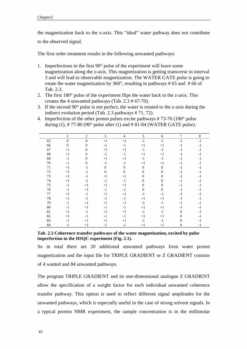
The first order treatment results in the following unwanted pathways:

1. Imperfections in the first 90° pulse of the experiment will leave some magnetization along the z-axis. This magnetization is getting transverse in interval 3 and will lead to observable magnetization. The WATER GATE pulse is going to rotate the water magnetization by 360°, resulting in pathways # 65 and # 66 of Tab. 2.3.

2. The first 180° pulse of the experiment flips the water back to the z-axis. This creates the 4 unwanted pathways (Tab. 2.3 # 67-70).

3. If the second 90° pulse is not perfect, the water is rotated to the z-axis during the indirect evolution period (Tab. 2.3 pathways # 71, 72).

4. Imperfection of the other proton pulses excite pathways # 73-76 (180° pulse during t1), # 77-80 (90° pulse after t1) and # 81-84 (WATER GATE pulse).

1 2 3 4 5 6 7 8

65 0 0 +1 +1 -1 -1 -1 -1 66 0 0 -1 -1 +1 +1 -1 -1 67 +1 0 +1 +1 -1 -1 -1 -1 68 +1 0 -1 -1 +1 +1 -1 -1 69 -1 0 +1 +1 -1 -1 -1 -1 70 -1 0 -1 -1 +1 +1 -1 -1 71 +1 -1 0 0 0 0 -1 -1 72 +1 -1 0 0 0 0 -1 -1 73 +1 -1 +1 +1 0 0 -1 -1 74 +1 -1 -1 -1 0 0 -1 -1 75 -1 +1 +1 +1 0 0 -1 -1 76 -1 +1 -1 -1 0 0 -1 -1 77 +1 -1 +1 +1 -1 -1 -1 -1 78 +1 -1 -1 -1 +1 +1 -1 -1 79 -1 +1 +1 +1 -1 -1 -1 -1 80 -1 +1 -1 -1 +1 +1 -1 -1 81 +1 -1 +1 +1 -1 -1 0 -1 82 +1 -1 -1 -1 +1 +1 0 -1 83 -1 +1 +1 +1 -1 -1 0 -1 84 -1 +1 -1 -1 +1 +1 0 -1

Tab. 2.3 Coherence transfer pathways of the water magnetization, excited by pulse imperfection in the HSQC experiment (Fig. 2.1).

So in total there are 20 additional unwanted pathways from water proton

magnetization and the input file for TRIPLE GRADIENT or Z GRADIENT consists

of 4 wanted and 84 unwanted pathways.

The program TRIPLE GRADIENT and its one-dimensional analogue Z GRADIENT

allow the specification of a weight factor for each individual unwanted coherence

transfer pathway. This option is used to reflect different signal amplitudes for the

unwanted pathways, which is especially useful in the case of strong solvent signals. In

a typical protein NMR experiment, the sample concentration is in the millimolar


43

range, while the water concentration is in the molar range. The water signal is

therefore 1000 to 10000 times stronger than any protein signal. Therefore an

optimized gradient sequence should suppress the unwanted water pathways more

efficiently.

Having decided which are the wanted and unwanted pathways, the free evolution

periods during which a gradient might be applied have to be specified in the input file

for the GRADIENT programs. Since in the present example we want to retain all

wanted pathways, there is no possibility to apply any effective gradient during the

indirect evolution time. If gradients are allowed during intervals 4 and 5 (Fig. 2.1), the

effect of the gradient in interval 5 refocuses the effect of the gradient in interval 4.

Since the wanted pathways have the same coherence order in intervals 4 and 5, the

two gradients are of the same amplitude, but have opposite sign.

Allowing gradients during intervals 3, 6, 7 and 8 leads to the suppression of all

unwanted pathways. Choosing less than four intervals results in the refocusing of

some unwanted pathways. The following discussion will focus on the results of

different optimization runs of TRIPLE GRADIENT and Z GRADIENT allowing

gradients during intervals 3, 6, 7 and 8 with different relative weights given to the

protein and the water pathways. The duration of each gradient is set to 1 ms.

After reading the input file, both programs calculate the selective, suppressive and

free subspaces by repeated application of the Gram-Schmidt procedure. The first

represents the subspace spanned by the wanted pathways, the second the subspace

spanned by the unwanted, whilst the free subspace is any remaining part of RF that can

be spanned neither by a wanted nor by an unwanted pathway. The condition that a

gradient sequence not perturbs the wanted signals can now be met simply by

generating it from within the suppressive and free subspaces. Details of the

computation are given in (Thomas, 1999).

In our example, we choose four intervals, so we are operating in R4. One basis vector

represents the wanted pathways and three orthogonal basis vectors represent the

unwanted pathways. The free subspace is empty. The orthonormal vectors constructed

by the Gram-Schmidt procedure are listed in Tab. 2.4. The three orthonormal base

vectors of the suppressive subspace are named A, B and C. The coherence order of the

Chapter2

44

wanted pathways during the zz-intervals is zero, so the vector representing the

selective subspace has zero components in the intervals 3 and 6.

free precession interval 3 6 7 8 vector representing desired pathways 0.00 0.00 0.71 -0.71 orthogonal vectors representing unwanted pathways

A 0.74 -0.67 0.00 0.00 B 0.67 0.74 0.00 0.00 C 0.00 0.00 0.71 0.71

Tab. 2.4 Components of the base vectors of the selective and suppressive subspace in the four selected intervals of the HSQC sequence of Fig. 2.1.

The components of all unwanted pathways in the suppressive subspace can now be

expressed as a linear combination of vectors A, B and C (x = a*A+b*B+c*C). The

expansion coefficients for all unwanted pathways are listed in Tab. 2.5. Only 19

independent vectors representing the unwanted pathways remain, if only those 4

intervals of free precession are chosen. The unwanted protein pathways are almost

restricted to the plane spanned by A and B, with the only exception of group 11 and

12 having a small component c. The corresponding pathways 57-64 are excited by

imperfections of the last 180° pulse on nitrogen (Previous page: Tab. 2.2).

Number group a B c 1-3. 19-21 1 1.49 0.00 0.00

16-18. 34-36 2 -1.49 0.00 0.00 37-39. 43-45 3 1.41 -0.07 0.00 40-42. 46-48 4 -1.41 0.07 0.00 10-12. 28-30 5 1.34 -0.13 0.00

7-9. 25-27 6 -1.34 0.13 0.00 50. 52. 54. 56 7 0.67 -0.74 0.00 49. 51. 53. 55 8 -0.67 0.74 0.00

4-6. 22-24 9 0.07 0.07 0.00 13-15. 31-33 10 -0.07 -0.07 0.00 58. 60. 62. 64 11 0.07 -0.07 -0.07 57. 59. 61. 63 12 -0.07 0.07 0.07

65. 67. 69. 77. 79 13 1.41 -0.07 -1.41 66. 68. 70. 78. 80 14 -1.41 0.07 -1.41

81. 83 15 1.41 -0.07 -0.71 82. 84 16 -1.41 0.07 -0.71 73. 75 17 0.74 0.67 -1.41 74. 76 18 -0.74 -0.67 -1.41 71. 72 19 0.00 0.00 -1.41

Tab. 2.5 Components a, b and c of the unwanted pathways in the base A, B, C. The numbers in the first column correspond to the numbers of the unwanted pathways in Tab. 2-11. Identical weight factors have been given to all pathways.


45

The relative weight of all pathways listed in Tab. 2.5 is equal to 1. The different

magnitudes of the vectors are mainly caused by their different magnitude of coherence

order during the zz-intervals. The weight factor just multiplies all components by a

constant specified for each pathway. The dependency of the optimized gradient

sequence for a one-dimensional gradient sequence on the weight factor for the water

pathways can be anticipated: The solution will be more and more driven to point

along base-vector C. The results of calculations using Z GRADIENT is summarized

in Tab. 2.7.

weights on water pathways

gradient strengths projection of gradients

#

3 6 7 8 a b c 0 1 43.85 -40.03 -32.15 -32.15 0.63 0.00 -0.37 1 2 43.18 -40.39 -29.76 -29.76 0.66 0.00 -0.34

1000 3 13.04 7.32 36.96 36.96 0.01 0.07 0.92 1000. 2000 4 10.90 6.21 37.10 37.10 0.01 0.05 0.95

10000 5 -6.12 -3.44 -36.78 -36.78 0.00 -0.02 -0.98 10000000 6 -0.62 -0.35 36.73 36.73 0.00 0.00 1.00 only water 7 0.00 0.00 -36.73 -36.73 0.00 0.00 -1.00

Tab. 2.6 Optimized z-gradients sequences for the HSQCzz-wg sequence (Fig. 2.1) calculated with Z-GRADIENT. The gradients strengths are listed in [ms*G/cm]. The normalized projections along the base-vectors A B and C are listed in the last three columns.

Having gradients around the WATERGATE pulse only optimizes water suppression.

In the base A, B, C this corresponds to applying a gradient in the direction of C only.

Any additional gradient component in the plane spanned by A and B will result in an

optimized suppression of the even numbered groups and lesser suppression of the odd

numbered groups of Tab. 2.5 and vice versa.

A three dimensional suppressive subspace is obviously very well suited for

application of gradients in three dimensions. The optimized gradient sequences for a

three-gradient system are listed in Tab. 2.7.

Chapter2

46

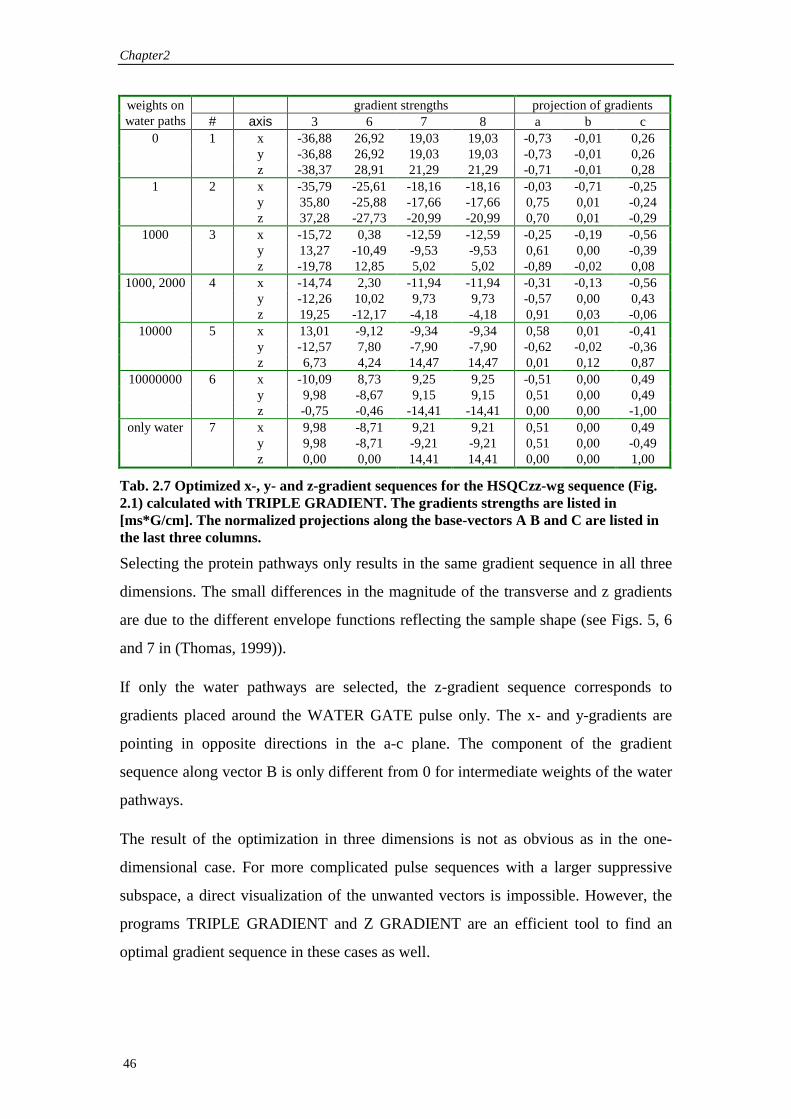
gradient strengths projection of gradients weights on water paths # axis 3 6 7 8 a b c

0 1 x -36,88 26,92 19,03 19,03 -0,73 -0,01 0,26 y -36,88 26,92 19,03 19,03 -0,73 -0,01 0,26 z -38,37 28,91 21,29 21,29 -0,71 -0,01 0,28

1 2 x -35,79 -25,61 -18,16 -18,16 -0,03 -0,71 -0,25 y 35,80 -25,88 -17,66 -17,66 0,75 0,01 -0,24 z 37,28 -27,73 -20,99 -20,99 0,70 0,01 -0,29

1000 3 x -15,72 0,38 -12,59 -12,59 -0,25 -0,19 -0,56 y 13,27 -10,49 -9,53 -9,53 0,61 0,00 -0,39 z -19,78 12,85 5,02 5,02 -0,89 -0,02 0,08

1000, 2000 4 x -14,74 2,30 -11,94 -11,94 -0,31 -0,13 -0,56 y -12,26 10,02 9,73 9,73 -0,57 0,00 0,43 z 19,25 -12,17 -4,18 -4,18 0,91 0,03 -0,06

10000 5 x 13,01 -9,12 -9,34 -9,34 0,58 0,01 -0,41 y -12,57 7,80 -7,90 -7,90 -0,62 -0,02 -0,36 z 6,73 4,24 14,47 14,47 0,01 0,12 0,87

10000000 6 x -10,09 8,73 9,25 9,25 -0,51 0,00 0,49 y 9,98 -8,67 9,15 9,15 0,51 0,00 0,49 z -0,75 -0,46 -14,41 -14,41 0,00 0,00 -1,00

only water 7 x 9,98 -8,71 9,21 9,21 0,51 0,00 0,49 y 9,98 -8,71 -9,21 -9,21 0,51 0,00 -0,49 z 0,00 0,00 14,41 14,41 0,00 0,00 1,00

Tab. 2.7 Optimized x-, y- and z-gradient sequences for the HSQCzz-wg sequence (Fig. 2.1) calculated with TRIPLE GRADIENT. The gradients strengths are listed in [ms*G/cm]. The normalized projections along the base-vectors A B and C are listed in the last three columns.

Selecting the protein pathways only results in the same gradient sequence in all three

dimensions. The small differences in the magnitude of the transverse and z gradients

are due to the different envelope functions reflecting the sample shape (see Figs. 5, 6

and 7 in (Thomas, 1999)).

If only the water pathways are selected, the z-gradient sequence corresponds to

gradients placed around the WATER GATE pulse only. The x- and y-gradients are

pointing in opposite directions in the a-c plane. The component of the gradient

sequence along vector B is only different from 0 for intermediate weights of the water

pathways.

The result of the optimization in three dimensions is not as obvious as in the one-

dimensional case. For more complicated pulse sequences with a larger suppressive

subspace, a direct visualization of the unwanted vectors is impossible. However, the

programs TRIPLE GRADIENT and Z GRADIENT are an efficient tool to find an

optimal gradient sequence in these cases as well.


47

The experimental water suppression of the calculated z-gradient and triple-gradients

sequences are shown in Fig. 2.2 and

Fig. 2.3. To avoid any effects from the phase cycling or partial saturation of the water

resonance during the pulse sequence, only one scan with the indirect chemical shift

dimension set to 3 µs, and no preceding dummy scan is shown. Any effects resulting

from the phase cycling or partial saturation of the water resonance during the pulse

sequence are therefore avoided and the efficiency of the water suppression of the

gradient sequence alone is monitored. The receiver gain was set to 512 for all

experiments. Gradients were applied with the shape of a half sine wave with the

gradient strength in percent of the maximum gradient strength as specified in Tab. 2.6

and Tab. 2.7. The first 1k points are recorded with a dwell time of 60 µs

corresponding to a total acquisition time of 61.44ms. This corresponds to a typical

acquisition time for protons in an experiment with 15N decoupling. The experiments

show that the water suppression is sufficiently good to allow a receiver gain of 512.

However, the theoretically predicted improvement of the gradient sequences with

respect to water suppression could not be confirmed.

The difference between calculated and observed water suppression rates is caused

mainly by radiation damping of the water signal (caused by the coupling of the rf-

circuit to the very strong water signal). The influence of radiation damping is seen

more clearly by looking at the full FID of the water signal, e.g. extending the

acquisition time to around 2s and changing the phase of the 90° proton pulse before

the second zz-interval to x. This results for example in an almost full recovery of the

water magnetization in trace 7 Fig. 2.1 of the z-gradient experiment with water-gate

gradients only. In this case, the water magnetization is flipped to the negative z-axis

by the last proton 90° pulse, where it stays until the acquisition is started. During the

acquisition period, the water is then brought to the transverse plane and back to the +z

axis by radiation damping.

Chapter2

48

Fig. 2.2 Comparison of the water suppression for different settings of the z-gradient strengths in the HSQC sequence of Fig. 2.1. The number on the right side of each trace corresponds to the number in column # of Tab. 2.6.

Fig. 2.3 Comparison of the water suppression for different settings of the x-, y- and z-gradient strengths in the HSQC sequence of Fig. 2.1. The number on the right side of each trace corresponds to the number in column # of Tab. 2.7.

If a number of dummy scans is applied before the data acquisition and the two step

phase cycle to select for 15N bound protons, the water suppression is found to be very

good for all of the calculated sequences. This means, that specifying the unwanted


49

pathways in the way introduced above leads to good water suppression almost

independent of the weight factors. Two spectra recorded with the optimized z-

gradients (Fig. 2.4) and triple-gradients (Fig. 2.5) show the efficiency of the water

gradient sequences. The spectra are recorded with four scans per t1 increment with a

relaxation delay of 1s between the scans on a 0.8 mM sample of the HRDC domain

(Liu, 1999) (80 amino acids). 256 indirect time increments were recorded in 19

minutes. The spectra have been multiplied with the decaying quarter of a squared sine

function in both dimensions and zero filled to a 2k x 1k data matrix prior to Fourier

transform. Both spectra are plotted on equal intensity contour levels. In addition, the

positive projection of all rows of the two-dimensional spectrum is shown on top of the

contour plot.

Chapter2

50

ppm

56789 ppm

80

85

90

95

100

105

Fig. 2.4 1H-15N HSQC spectrum of a 0.8 mM protein sample in H2O recorded with the pulse-sequence of Fig. 2.1. The spectrum was recorded with 4 scans for each t1 increment and a recycle delay of 1s. The z-gradient strength in % was set to 13.04, 7.32, 36.96 and 36.96 for the four gradients.


51

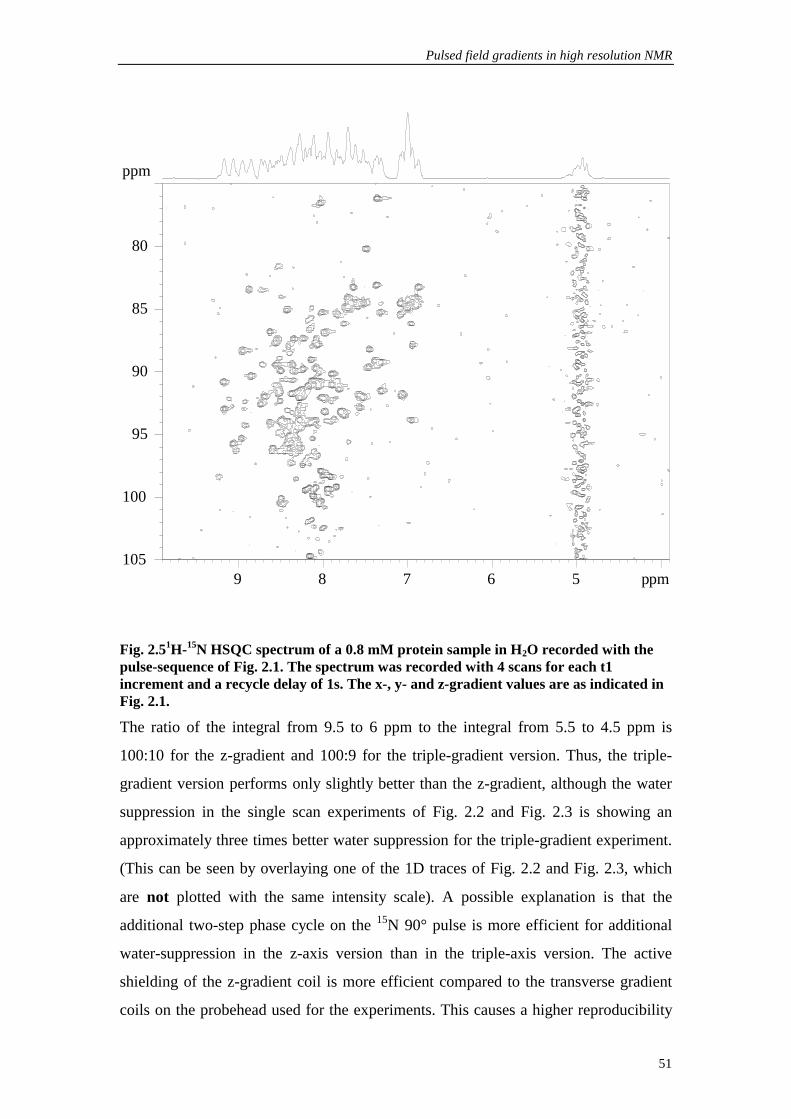
Fig. 2.51H-15N HSQC spectrum of a 0.8 mM protein sample in H2O recorded with the pulse-sequence of Fig. 2.1. The spectrum was recorded with 4 scans for each t1 increment and a recycle delay of 1s. The x-, y- and z-gradient values are as indicated in Fig. 2.1.

The ratio of the integral from 9.5 to 6 ppm to the integral from 5.5 to 4.5 ppm is

100:10 for the z-gradient and 100:9 for the triple-gradient version. Thus, the triple-

gradient version performs only slightly better than the z-gradient, although the water

suppression in the single scan experiments of Fig. 2.2 and Fig. 2.3 is showing an

approximately three times better water suppression for the triple-gradient experiment.

(This can be seen by overlaying one of the 1D traces of Fig. 2.2 and Fig. 2.3, which

are not plotted with the same intensity scale). A possible explanation is that the

additional two-step phase cycle on the 15N 90° pulse is more efficient for additional

water-suppression in the z-axis version than in the triple-axis version. The active

shielding of the z-gradient coil is more efficient compared to the transverse gradient

coils on the probehead used for the experiments. This causes a higher reproducibility

ppm

56789 ppm

80

85

90

95

100

105

Chapter2

52

of the water signal in different scans of the z-gradient version and thus a more

efficient cancellation of the water resonance by subtraction of alternate scans in the

acquisition buffer. Trial and error optimizations of the gradient sequences by an

experienced user performed typically about 5 % worse giving an intensity ratio of the

integrated signal to the water in the positive projection of 100:15.

These experiments show that the above treatment of the water-signal in the

development of sequences of pulsed field gradients leads to satisfactory water-

suppression and artifact reduction. A rather simple example of the four gradients in

the HSQC water-gate sequence is chosen because it allows a relative nice pictorial

representation of the calculated gradient sequences in terms of the geometric

approach.

It was found to be important to treat possible pulse imperfections in a consistent way –

especially for the strong water signal. With the approach outlined in this section, a

simple and straightforward way of dealing with imperfections is being presented. The

approach depicted here is expected to work well, if unwanted signals arise from pulse

imperfections only. Any considerations concerning different spin systems and

coupling patterns have been discarded for simplicity. Any unwanted signals arising

from different spin topologies should be identified via a product operator analysis. In

the case of protein NMR this is usually straight forward, since the coupling patterns

and chemical shift ranges for the 20 amino acids are very well known. In cases where

unwanted signal intensities arising from different spin systems have equal or higher

intensities as the wanted signals, pulse imperfections for these "ideal" unwanted

pathways can be treated accordingly.

In a more general approach all possible pathways that could be created by any spin

system would have to be considered. This would create a large number of pathways –

for example there are 151,875 pathways reported in the case of a HSQC sequence

(Jerschow, 1998). Such a large number of unwanted pathways are difficult to handle

by TRIPLE GRADIENT or Z GRADIENT, even if many pathways could be rejected

as redundant for a limited selection of intervals during which pulsed field gradients

were to be applied. The main advantage of doing a selection of unwanted pathways is

that the optimized gradient sequence suppresses those especially well. Adding more

pathways, which do not contribute significantly to the detected signal, might result in


53

a gradient sequence, which would not be as efficient in suppressing the strong

unwanted signals.

The selection of significant unwanted pathways could be done automatically by using

the approach outlined in (Jerschow, 1998). If a pulse sequence without any gradients

is given to the program outlined by Jerschow and Müller, the most significant

remaining pathways and their transfer amplitudes are returned and could be fed

directly into the gradient optimization of TRIPLE GRADIENT or Z GRADIENT.

This approach is also expected to be very robust. However, neglecting any transfer

amplitudes by not using any information about the spin topology as done in the

approach of (Jerschow, 1998) might again lead to the inclusion of unwanted pathway

with negligible contributions. On the other hand, a full automation of the selection of

unwanted pathways reduces the problem to a purely technical one.

Having artifact free spectra is especially important in cases where quantitative

measurements are to be performed. The identification of artifacts in HSQC spectra

and their removal was done during the setup of experiments for an investigation of the

dynamics of the PH domain of β-spectrin (Gryk, 1998). The changes of the internal

dynamics of the PH domain by ligand binding are very subtle and we found that high

quality spectra were a prerequisite for their observation.

2.4 Diffusion in multi-pulse heteronuclear experiments

2.4.1 General expressions for the signal attenuation by rectangular and sine shaped gradients

In section 2.2 we get two general expressions (Eqs. (2.24) and (2.25)) for the influence

of diffusion on the attenuation of a coherence order transfer pathway. This chapter is

going to give some specific solutions to these equations. The equation in the time

domain (2.25) is more straightforward to solve directly without any assumptions about

the gradient pulse sequence. The integral is split into F integrals over the time

intervals ∆i between the end point of two consecutive pulsed field gradients (see Fig.

2.6). The coherence order does not change during each of the gradients and two

consecutive gradients are separated by one or more rf-pulses. The gradient shapes are

specified explicitly by the shape factors fαi. The shape factors considered are

Chapter2

54

rectangular and the first half of a sine wave, which are the shape factors most widely

used in high resolution experiments.

Rectangular gradients

First we are going to treat the case of rectangular gradients with the same shape f for

the three Cartesian dimensions α, e.g.

( ) otherwise

ttftf iiii

≤≤−

==

01

)(τδτ

α ( 2.32 )

A schematic figure of the sequence of pulsed field gradient is given in Fig. 2.6

Fig. 2.6 Schematic representation of a series of rectangular pulsed field gradients. Between the end of one gradient and the beginning of the next, one or a series of rf-pulses is applied, which lead to changes in the coherence order pi.

The solution of (2.25) during the time interval ∆i divides into two parts: the time δi

with the effective gradient of Gipi is on and the remaining time with zero gradient.

The first part gives:


55

( )( )

( ) ( ) ( )( )( )

( ) ( ) ( ) ( ) ( )

( ) ( )

δ+δ+δγ=

δ−τ−+δ−τ−+γ=

δ−τ−+δ−τ−+γ=

δ−τ−+γ=

′+γ

αα−

α−−

α−

τ

δ−τ

αα−

α−−

α−

τ

δ−ταα

−α

−−α

−

τ

δ−τα

−α

−

τ

δ−τ δ−ταα

−

=

∫

∫

∫ ∫∑

3GpGp

3)(uGp

2)(uGp2u

du )(uGp)(uGp2

du)(uGp

du tdGpsp

3i2ii2

iii1i1i

i21i1i2

I

3ii2ii

2iiii1i1i21i1i2

I

2ii

iiii

ii1i1i21i1i2I

2

iiii1i1i2

I

2u

iij1i

1j

jI

i

ii

i

ii

i

ii

i

ii ii

spsp

spsp

spsp

sp

( 2.33 )

where we have written

∑−

=

−α

−α =

1i

1r

1i1irrsp sp ( 2.34 )

for simplicity.

The second part of the integration over the time interval ∆i is independent of the

gradient shape function equal to

( ) ( )ii21i1i

I

2r

1i

1r

rI dusp

ii

ii

δ−∆γ=γ −α

−δ−τ

∆−τα

−

=∫ ∑ sp ( 2.35 )

Introducing the wavevectors ki-1 and hi, defined in analogy to (2.15)

γ=

γ= ∑−

=−

iz

iy

ix

iIi

1i

1r rz

ry

rx

rI1i

sss

psss

p h k ( 2.36 )

The attenuation of a coherence transfer pathway during the interval ∆i is given by

adding the two contributions (2.33 ) and (2.35)

( ) ( ) ( ) ( )

δ+δ+∆−= −− 3

DexpS

S i2iii1ii

21i

0

i hhkkk ( 2.37 )

where we have assumed isotropic diffusion for simplicity.

There are three contributions to the signal attenuation during the interval ∆i:

Chapter2

56

1. The first factor corresponds to a decay that is linear in time. The time interval ∆i starts at the end of gradient i and ends at the end of the next gradient i+1. At the end of the integral i each coherence pathway p has accumulated a phase ~Σpisi corresponding to a wavevector ki. The wavelength λ i=2πki

-1 corresponds to a real spatial modulation of the magnetization in the sample. Thus a magnetization grid (Kimmich, 1997; Simon, 1996) or grating (Sodickson, 1998) is present in all three spatial dimensions. The influence of the diffusion is to reduce the amplitude of this magnetization grid by a factor exp(-D(kir0)2∆i).

2. The third factor is proportional to the third power of the gradient pulse length. It depends on the coherence order during interval i and the gradient strength only, and is especially independent of any gradients applied before interval i. Due to the square, this factor is always positive leading to a signal decay. It corresponds to the unavoidable signal loss in the presence of a gradient.

3. The second factor is proportional to the product of the wavevector present before the gradient i with the gradient strength of gradient i. The sign of the product depends on the relative sign of ki-1 and hi. If hi and ki-1 have opposite signs this factor is negative and thus increases the signal amplitude. In words of the magnetization grid, hi and ki-1 having opposite sign means that the gradient i starts to unwind the magnetization grid present over the sample.

The summation over all intervals i of the pulse-sequence results in an attenuation

factor, which is just the product of the attenuation, factors for single intervals.

( ) ( ) ( ) ( )

δ+δ+∆−Π= −−= 3

DexpS

S i2iii1ii

21i

F

1i0

hhkkk ( 2.38 )

The wavevector k0 = 0 is introduced in this formula for simplicity. If diffusion during the gradients is neglected, e. g. taking the shape-function f to be the

δ-function reproduces the result in (Jerschow, 1998). Using (2.38), the echo

attenuation in pulsed field gradient stimulated echo experiments (Stejskal and Tanner,

1965) and the bipolar (Wu, 1995) or convection compensated (Jerschow, 1997)

variants are easily derived.


57

Sine shaped gradients

Very often the shape of the pulsed field gradients is smoothed, to reduce the

mechanical momentum on the gradient coil during the switching. (The strong

mechanical force on the probe manifests itself in a hearable clicking, when pulsed

field gradients are applied.) A very popular shape is to use the first lobe of a sine

wave:

( )

τ≤≤δ−τ

δ+τ−

δπ

==α

otherwhise0

t)t(sin)t(ftf iiiiii

i ( 2.39 )

The diffusion during the gradient is obtained in analogy to (2.33)

( ) ( )

πδ+

πδ+δγ=

′

δ+τ−

δπ+γ

αα−

α−−

α−

τ

δ−τ δ−ταα

−

=∫ ∫∑

2

3i2ii

2iii1i1i

i21i1i2

I

2u

iii

iir1i

1r

rI

23Gp2Gp

du td)t(sinGpspi

ii ii

spsp

( 2.40 )

The strength of a single sine-gradient is

πδ=′

′

δπ= ∫

δ 2Gt dtsinGs0

( 2.41 )

The overall attenuation during a pulse sequence due to diffusion is

( ) ( ) ( )

++∆−Π= −−= iiiiiii

F

iD

SS δδ

83exp 2

12

110

hhkkk ( 2.42 )

which looks basically the same as in the case of rectangular gradients except for the

factor 3/8 in the diffusion during the pulsed field gradients instead of 1/3 in (2.38).

Solutions for sine-shaped gradients given for a pulsed field gradient spin echo

experiment with two gradient pulses (Merrill, 1993; Price and Kuchel, 1991) are

reproduced by Eq. (2-42).

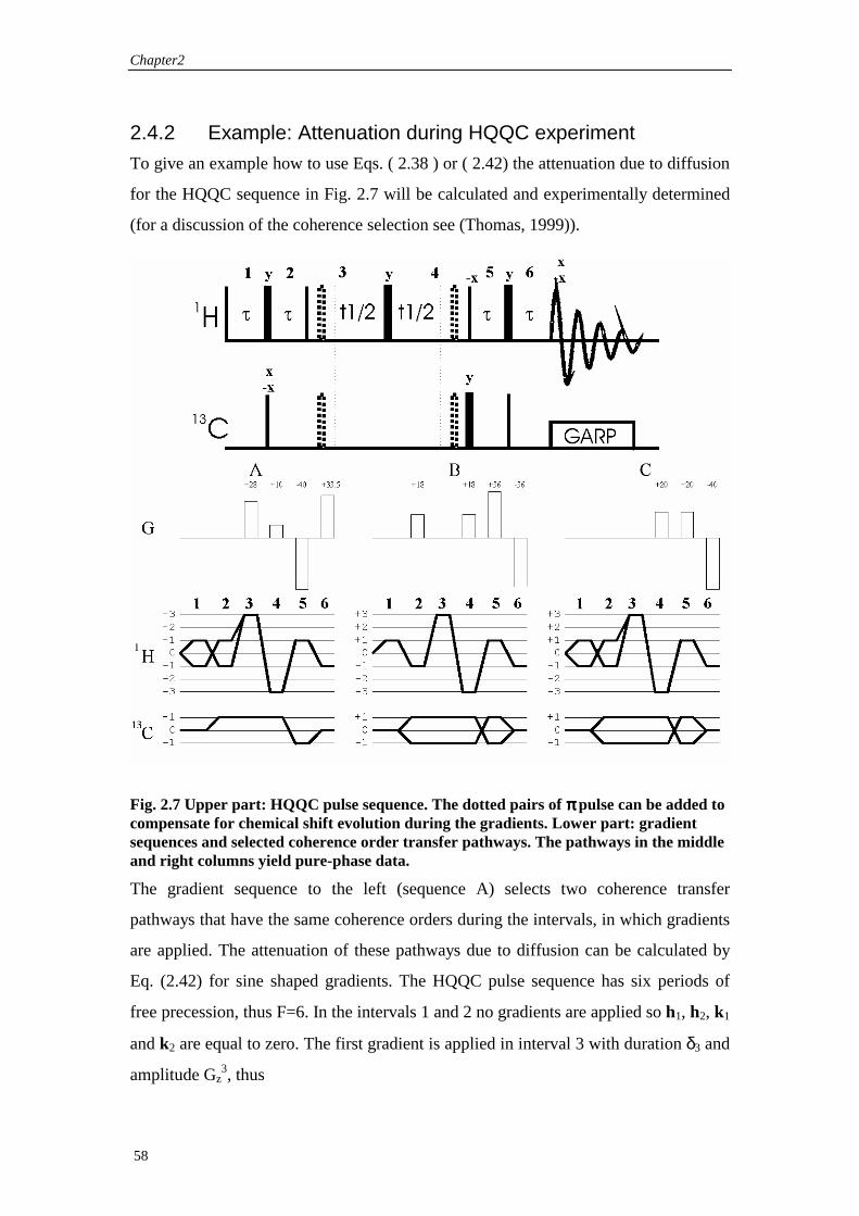
Chapter2

58

2.4.2 Example: Attenuation during HQQC experiment To give an example how to use Eqs. ( 2.38 ) or ( 2.42) the attenuation due to diffusion

for the HQQC sequence in Fig. 2.7 will be calculated and experimentally determined

(for a discussion of the coherence selection see (Thomas, 1999)).

Fig. 2.7 Upper part: HQQC pulse sequence. The dotted pairs of ππππ pulse can be added to compensate for chemical shift evolution during the gradients. Lower part: gradient sequences and selected coherence order transfer pathways. The pathways in the middle and right columns yield pure-phase data.

The gradient sequence to the left (sequence A) selects two coherence transfer

pathways that have the same coherence orders during the intervals, in which gradients

are applied. The attenuation of these pathways due to diffusion can be calculated by

Eq. (2.42) for sine shaped gradients. The HQQC pulse sequence has six periods of

free precession, thus F=6. In the intervals 1 and 2 no gradients are applied so h1, h2, k1

and k2 are equal to zero. The first gradient is applied in interval 3 with duration δ3 and

amplitude Gz3, thus


59

=

=

===′

′= ∫

πδ

γγ

πδ

δπδ

33

3

3

33

3333

0 3

33

200

00

02sin3

z

I

z

I

yxzzz

Gp

sp

ssGtdtGs

h

For the following intervals 4, 5 and 6, the corresponding wavevectors are given by

++=++===

+=+===

====

πδ

πδ

πδγ

πδγ

πδ

δπδδ

πδγ

πδγ

πδ

πδγ

πδγ

πδ

55544433354356666666

4344

33334345555555

333334444444

22222

2222

222

zzzIzzzzzIzzz

zzIzzzzIzzz

zIzzzIzzz

GpGpGphhhkGphGs

GpGphhkGphGs

GphkGphGs

Assuming that all pulsed field gradients have the same length δ, the overall

attenuation factor is given by

( ) ( ) ( )

( ) ( ) ( )[ ]

( )( ) ( )( ) ( )( )[ ]

( ) ( ) ( ) ( )[ ]

+++

−

⋅

+++++

−

⋅

∆+++∆++∆

−=

++∆−Π= −−=

2662552442332

6655443355443344332

62554433

524433

4233

2

21

211

0

32exp

2exp

2exp

83exp

zzzzI

zzzzzzzzzI

zzzzzzI

iiiii

F

i

GpGpGpGpD

GpGpGpGpGpGpGpGpGpD

GpGpGpGpGpGpD

DS

S

δπδγ

δπδγ

πδγ

δδ

hhkkk

Plugging in the numbers for the gradient amplitudes G (in % of the maximum

gradients strength g) and the coherence orders p, this is equal to

( ) ( )

[ ]

−∆+∆+∆

−=

++++

++−∆+∆+∆

−=

δπδγ

δ

δπδγ

14.011.040.083.02exp

)]11.009.008.082.0(8

3

11.019.025.011.040,083.0[2exp

654

2

654

2

0

I

I

gD

gDS

S

k

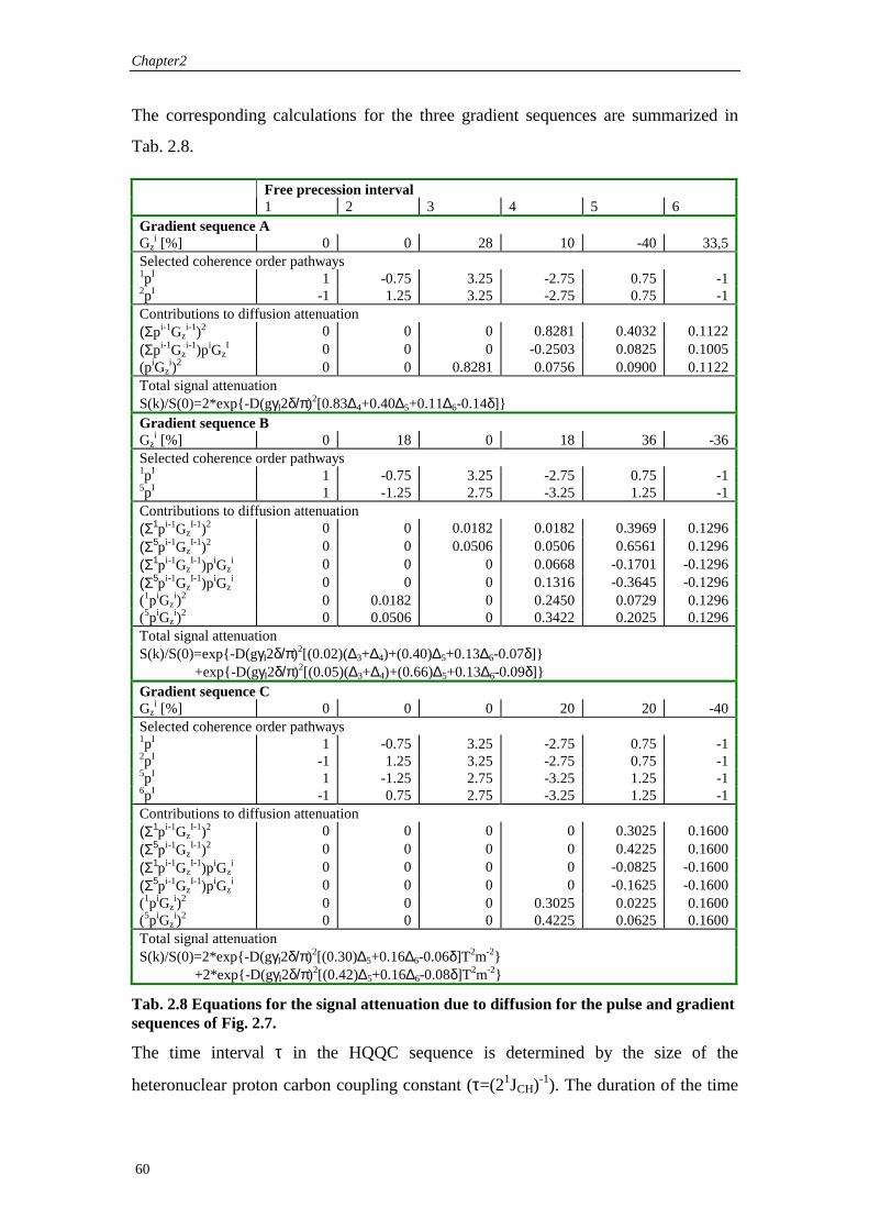
Chapter2

60

The corresponding calculations for the three gradient sequences are summarized in

Tab. 2.8.

Free precession interval 1 2 3 4 5 6 Gradient sequence A Gz

i [%] 0 0 28 10 -40 33,5 Selected coherence order pathways 1pI 1 -0.75 3.25 -2.75 0.75 -1 2pI -1 1.25 3.25 -2.75 0.75 -1 Contributions to diffusion attenuation (Σpi-1Gz

i-1)2 0 0 0 0.8281 0.4032 0.1122 (Σpi-1Gz

i-1)piGzI 0 0 0 -0.2503 0.0825 0.1005

(piGzi)2 0 0 0.8281 0.0756 0.0900 0.1122

Total signal attenuation S(k)/S(0)=2*exp-D(gγI2δ/π)2[0.83∆4+0.40∆5+0.11∆6-0.14δ] Gradient sequence B Gz

i [%] 0 18 0 18 36 -36 Selected coherence order pathways 1pI 1 -0.75 3.25 -2.75 0.75 -1 5pI 1 -1.25 2.75 -3.25 1.25 -1 Contributions to diffusion attenuation (Σ1pi-1Gz

I-1)2 0 0 0.0182 0.0182 0.3969 0.1296 (Σ5pi-1Gz

I-1)2 0 0 0.0506 0.0506 0.6561 0.1296 (Σ1pi-1Gz

I-1)piGzi 0 0 0 0.0668 -0.1701 -0.1296

(Σ5pi-1GzI-1)piGz

i 0 0 0 0.1316 -0.3645 -0.1296 (1piGz

i)2 0 0.0182 0 0.2450 0.0729 0.1296 (5piGz

i)2 0 0.0506 0 0.3422 0.2025 0.1296 Total signal attenuation S(k)/S(0)=exp-D(gγI2δ/π)2[(0.02)(∆3+∆4)+(0.40)∆5+0.13∆6-0.07δ] +exp-D(gγI2δ/π)2[(0.05)(∆3+∆4)+(0.66)∆5+0.13∆6-0.09δ] Gradient sequence C Gz

i [%] 0 0 0 20 20 -40 Selected coherence order pathways 1pI 1 -0.75 3.25 -2.75 0.75 -1 2pI -1 1.25 3.25 -2.75 0.75 -1 5pI 1 -1.25 2.75 -3.25 1.25 -1 6pI -1 0.75 2.75 -3.25 1.25 -1 Contributions to diffusion attenuation (Σ1pi-1Gz

I-1)2 0 0 0 0 0.3025 0.1600 (Σ5pi-1Gz

I-1)2 0 0 0 0 0.4225 0.1600 (Σ1pi-1Gz

I-1)piGzi 0 0 0 0 -0.0825 -0.1600

(Σ5pi-1GzI-1)piGz

i 0 0 0 0 -0.1625 -0.1600 (1piGz

i)2 0 0 0 0.3025 0.0225 0.1600 (5piGz

i)2 0 0 0 0.4225 0.0625 0.1600 Total signal attenuation S(k)/S(0)=2*exp-D(gγI2δ/π)2[(0.30)∆5+0.16∆6-0.06δ]T2m-2 +2*exp-D(gγI2δ/π)2[(0.42)∆5+0.16∆6-0.08δ]T2m-2

Tab. 2.8 Equations for the signal attenuation due to diffusion for the pulse and gradient sequences of Fig. 2.7.

The time interval τ in the HQQC sequence is determined by the size of the

heteronuclear proton carbon coupling constant (τ=(21JCH)-1). The duration of the time


61

intervals ∆3-∆6 depends on the position of the gradients during the free precession

periods. This will determine which of the intervals ∆3-∆5 change by incrementing the

indirect evolution interval (remember that the interval ∆i ends at the end of the

gradient placed in the free precession period i).

For gradient sequence B and C the coherence orders of the selected pathways are not

equal during the intervals of free precession with applied gradient. The corresponding

pathways are attenuated differently. Gradient sequences B and C select +0.25 and -

0.25 carbon coherence order during the indirect evolution interval t1. The two

pathways (p- and n-type) are necessary to get pure phase spectra in ω1.

As experimental example, HQQC spectra of ethanol in D2O were recorded using

gradient sequences A, B and C. All sequences select the signal of the 13C bound

methyl protons efficiently (see Fig. 2.8). The t1-ridge at the position of the 12C bound

methyl-proton resonance in gradient sequence B is caused mainly by instabilities of

the gradient unit during some of the FIDs between t1=40ms and t1=80ms. The

inspection of the signal decay with respect to t1 shows immediately the strong

influence of diffusion in gradient sequence A. The additional modulation of the

signals is caused by small proton-proton couplings of the methyl and methylene

protons. After two-dimensional Fourier transform, pure absorption peaks in both

dimensions are observed in gradient sequence B and C, because they select p- and n-

type coherence orders in t1 simultaneously. The intensity of the signals reflects

approximately the different number of coherence transfer pathways selected. To make

a quantitative comparison, the magnitude of the two-dimensional spectrum was

calculated, and all points within a box around the signals were summed up. The

resulting volume ratios are 1.0 : 1.2 : 2.2 for sequence A : B : C.

Chapter2

62

Fig. 2.8 Natural abundance 13C HQQC experiment of ethanol in D2O (containing a trace of CuSO4 to enhance relaxation) using the pulse sequence in Fig. 2.7 with the optional pairs of ππππ pulses during t1. Upper row: two-dimensional interferogram obtained after Fourier transformation with respect to the acquisition dimension. Lower trace: methyl region of the 2D spectrum. The spectra have acquired with the same number of transients, are processed identically and plotted with using the same (positive) contour levels.

The strongest influence of diffusion is observed in gradient sequence A. The first

gradient is applied during a period were quadruple quantum coherence is excited,

leading to a multiplication factor of 3.25 in the calculation of the effective gradient

strength. The magnetization grid produced by this gradient is refocused only after the

indirect evolution time t1. In gradient sequence B the attenuation during t1 is much

less because the first gradient is applied in an interval during which heteronuclear

double quantum coherence is excited. The attenuation in gradient sequence C is

independent of t1 since the first gradient is applied after the indirect evolution period.


63

The difference in linewidth between the signals in the indirect dimension of spectra A

and C can be used directly to determine the diffusion coefficient of ethanol. The signal

decay in sequence C is governed by transverse relaxation only, while the additional

linewidth in sequence A and B is caused by diffusion. The linewidth of the signals in

ω2 was determined by fitting a Lorentzian to one-dimensional traces of the spectrum.

The obtained values are 5.9 Hz (A), 3.7 Hz (B) and 3.6 Hz (C).

To point out the similarity between the signal loss by relaxation and diffusion, a

"diffusional relaxation rate Rd=1/Td” might be introduced. The interval ∆4 in the

above notation is proportional to t1, and the signal decay in dependence of t1 is (see

Tab. 2.8)

Rd= 0.83 D (gγI2δ/π)2

for gradient sequence A. From the experimentally determined difference of 2.3 Hz

between spectrum A and C a diffusional relaxation rate Rd=π∆ν of 7.2 s-1 results.

With the maximum gradient strength of the probehead g= 0.56 T/m, the gradient

duration δ=1ms and the gyromagnetic ratio of the protons γI=2.675 108radT-1s-1, the

diffusion coefficient for ethanol is determined to be 0.96 10-9 m2s-1. This compares to

1.02 10-9 m2s-1 obtained on the same sample with a stimulated echo sequence.

2.5 Discussion Gradient selection of coherence transfer pathways must meet several practical

requirements to be useful for routine NMR spectroscopy. Most importantly, the

gradient sequences should guarantee that the actual NMR experiment is the one

required, in the sense that only wanted signals are captured and simultaneously the

unwanted ones are suppressed. The optimum solution to this problem depends on

additional requirements, like maximizing the signal-to-noise ratio, obtaining pure-

phase spectra in the indirect dimension, reducing the experimental time or suppressing

artifacts efficiently. Not all of these criteria can be fulfilled optimally at the same time,

for example maximizing signal-to-noise and reducing the experimental time are

mutually exclusive, and so the selection of a particular sequence of pulsed field

gradients depends on the specific application.

Chapter2

64

The computer programs TRIPLE GRADIENT and Z GRADIENT are powerful tools

for the design of optimal sequences of pulsed field gradients. The number and kind of

pathways to be selected or suppressed are chosen by the spectroscopist, and the

programs then determine whether or not any appropriate gradient sequence exists. The

programs can also be used iteratively, as described in a previous publication (Thomas,

1999), where we focus on the optimization of signal-to-noise ratio for an experiment,

which excites high order coherence. The process of selecting an optimal subset of the

coherence transfer pathways is outlined, which allows to record pure phase absorption

peaks in the indirect dimension without any special processing.

In chapter 2.3 of this thesis, a different aspect of the design of gradient pulse

sequences is addressed, namely the suppression of artifacts. With the aid of the

programs TRIPLE GRADIENT and Z GRADIENT, this can be achieved after

identifying the coherence transfer pathway causing the artifact. The computer

programs are able to find a gradient sequence, which suppresses the unwanted

pathways optimally, while the wanted signal is fully retained in cases where this is

possible.

The main source of systematic artifacts in NMR spectra are imperfections of π pulses.

To find the resulting unwanted pathways, we expand the pulse flip angle in a Taylor

series around its nominal value and consider only the linear term. This reduces the

number of unwanted pathways considerably, but retains the most important ones. For

the solvent signal, the same approach is extended to all pulses and different weight

factors reflecting the intensity difference of solvent and protein signal are tested. The

calculated gradient sequences produce artifact free spectra with very good water

suppression. The residual small water signal is caused mainly by radiation damping

(which is the direct coupling of the strong water magnetization to the resonance circuit

of the probehead). For further improvements of the gradient sequences it is necessary

to add unwanted pathways created by radiation damping rather than including

pathways caused by second order deviations of the pulse flip angles.

The application of pulsed field gradients leads to a spatial phase dependence, which is

determined by the gradient sequence and the coherence orders during the experiment.

The selection of a particular coherence transfer pathway is equivalent to the condition

that this spatial dependence is refocused before signal acquisition and thus a gradient


65

echo is formed. The intensity and phase of the selected signals are changing, if the

molecules undergo motion during the experiment. The theoretical part outlined in

chapter 2.2 includes a very general formulation to include motional effects and

following the treatment of Stepisnik (Stepisnik, 1981; Stepisnik, 1985) the equations

are further analyzed using the cumulant expansion theorem.

The influence of unrestricted diffusion on the signal amplitudes in an arbitrary pulse

sequence with sine pulsed field gradients (including constant gradients as a special

case of a sequence of rectangular gradients with constant amplitude and no spacing) is

evaluated for the first time in a general and exact way in chapter 2.4. Previously used

approximations, as for example neglecting diffusion during the gradients (Jerschow,

1998), are unnecessary since the exact calculation does not require significantly more

computation time.

In the experimental examples different aspects of signal selection and signal

attenuation by diffusion are shown in a pulse sequence selecting heteronuclear

quadruple quantum coherence. The relative signal volumes in spectra recorded with

different sequences of pulsed field gradients in an otherwise identical pulse sequence

is determined by the different numbers of coherence transfer pathways selected. Pure

absorption peaks shapes in the spectra are only obtained of p- and n-type coherences

are selected simultaneously. The signal decay in the indirect dimension is determined

by transverse relaxation and diffusion. The diffusion constant of ethanol is reproduced

with an accuracy of 10% from the difference in linewidth observed in the spectra.

It is expected that the formalism is going to be helpful for the design of pulse

sequences to measure diffusion. The formal introduction of a “diffusional relaxation”

time Td makes clear that such experiments might use the same principles as used for

the measurement of transverse or longitudinal relaxation times. Intervals used to

encode for chemical shift can be used simultanesously to determine diffusion

constants. In the experimental example (chapter 2.4.2) the separation of diffusion and

relaxation effects is achieved by evaluating the difference of two experiments.

Alternatively, a constant time chemical shift interval can be used in between gradients

encoding for diffusion. If now the gradient strength and the chemical shift evolution

are varied in a concerted manner, the diffusion coefficient is determined directly from

the observed linewidth of the signals as in the so-called accordion approach for

Chapter2

66

measuring relaxation (Ernst, 1987). This would allow the separation of signals of

different molecules in a mixture based on the diffusion coefficient from one two-

dimensional experiment and thus making use of the higher resolution of the two-

dimensional spectrum without extra experimental time needed for the variation of the

strength of a diffusion encoding gradient used in proposed experiments (Barjat et al.,

1998).

To improve the calculation of optimized sequences of pulsed field gradients, the

influence of diffusion could be added to the penalty function of TRIPLE GRADIENT

and Z GRADIENT. This should lead to better results in two different ways: (1) The

diffusion losses for the wanted signals are minimized. (2) The suppression of solvent

is optimized by making use of the faster diffusion of the solvent molecules compared

to the molecules of interest.

The theory is formulated to allow arbitrary random or coherent motion for the spins.

This makes it possible to include other motional effects than unrestricted diffusion.

An analytical solution of the influence of the gradients on signal amplitude and phase

is impossible in most cases and approximations have to be introduced, the most

common one being the narrow (gradient) pulse approximation (Callaghan, 1991).

Examples for expressions for pulsed gradient and double pulsed gradient stimulated

echo experiments are found in ( Callaghan, 1999 ).

2.6 References Aliteri, A.S., Miller, K. E. and Byrd, R. A. (1996) A comparison of water suppression techniques using

pulsed field gradients for high-resolution NMR of biomolecules. Magn. Reson. Rev., 17, 27-82.

Aue, W.P., Bartholdi, E. and Ernst, R.R. (1976) Two-dimensional spectroscopy. Application to nuclear magnetic resonance. J. Chem. Phys., 64, 2229-2246.

Bain, A.D. (1984) Coherence Levels and Coherence Pathways in NMR. A simple Way to design Phase Cycling Procedures. J. Magn. Reson., 56, 418.

Barjat, H., Morris, G.A. and Swanson, A.G. (1998) A three-dimensional DOSY-HMQC experiment for the hig-resolution analysis of comples mixtures. J. Magn. Reson., 131, 131-138.

Bax, A.and Pochapsky, S. S. (1992) Optimized recording of heteronuclear multidimensional NMR spectra using pulsed field gradients. J. Magn. Reson., 99, 638-643.

Blümich, B., Blümler, P., Botto, R. and Fukushima, E. (1998) Spatially resolved magnetic resonance. Wiley-VCH, Weinheim.

Bodenhausen, G., Koegler, H. and Ernst, R. R. (1984) Selection of Coherence-Transfer Pathways in NMR Pulse Experiments. J. Magn. Reson., 58, 370.


67

Brondeau, J., Boudot, D., Mutzenhardt, P and Canet, D. (1992) The equivalent of the DQF-COSY experiment, with one transient per t1 value, by use of B1 gradients. J. Magn. Reson., 100, 611-618.

Callaghan, P.T. (1991) Principles of Nuclear Magnetic Resonance Microscopy. Oxford University Press, Oxford.

Callaghan, P.T. and Stepisnik, J. (1995) Frequency-domain analysis of spin motion using modulated-gradient NMR. J. Magn. Reson. Ser. A, 117, 118-122.

Callaghan, P.T., Codd, S.L. and Seymour, J.D. (1999) Spatial coherence phenomena arising from translational spin motion in gradient spin echo experiments. Conc. Magn. Reson., 11, 181-202.

Canet, D. (1997) Radiofrequency field gradient experiments. Prog. NMR spectr., 30, 101-135. Carr, H.Y. and Purcell, E.M. (1954) Effects of diffusion on free precession in nuclear magnetic

resonance experiments. Phys. Rev., 94, 630-638. Cavanagh, J., Fairbrother, W. J., Palmer III, A. G. and Skelton, N. J. (1996) Protein NMR spectroscopy

- principles and practice. Academic Press, San Diego. Cavanagh, J., Palmer III, A.G., Wright, P.E. and Rance, M. (1991) Sensitivity improvement in proton-

detected two-dimensional heteronuclear relay spectroscopy. J. Magn. Reson., 91, 429-36. Counsell, C.J.R., Levitt, M. H. and Ernst, R. R. (1985) The selection of coherence-transfer pathways by

inhomogeneous z pulses. J. Magn. Reson., 64, 470-478. Czisch, M., Ross, A., Cieslar, C. and Holak, T.A. (1996) Some practical aspects of B0 gradient pulses.

J. Biomol. NMR, 7, 121-130. Ernst, R.R. and Anderson, W.A. (1966) Rev. Sci. Instr., 37, 93-102. Ernst, R.R., Bodenhausen, G. and Wokaun, A. (1987) Principles of Nuclear Magnetic Resonance in

One and Two Dimensions. Clarendon Press, Oxford. Gardiner, C.W. (1983) Handbook of stochastic methods. Springer, Berlin. Gryk, M.R., Abseher, R., Simon, B., Nilges, M. and Oschkinat, H. (1998) Heteronuclear relaxation

study of the PH domain of β-spectrin: Restriction of loop motions upon binding inositol trisphosphate. J. Mol. Biol., 280, 879-896.

Hahn, E.L. (1950) Spin Echos. Phys. Rev., 80, 580-594. Hammarström, A.and Otting, G. (1994) Axial-peak artifacts in multipulse NMR experiments. J. Magn.

Reson. A, 109, 246-249. Hore, P.J. (1989) In N. J. O. a. T. L. James (ed.) Nuclear magnetic resonance. Solvent suppression.

Academic Press, San Diego, Vol. 176, pp. 64. Hoult, D.I. (1979) Rotating Frame Zeugmatography. J. Magn. Reson., 33, 183-197. Humbert, F., Valtier, M., Retournard, A. and Canet, D. (1998) Diffusion measurements using

radiofrequency field gradient: artifacts, remedies, practical hints. J. Magn. Reson., 134, 245-254.

Hurd, R.E. (1990) Gradient-enhanced spectroscopy. J. Magn. Reson., 87, 422. Hurd, R.E., Boban, K. J., Webb, P. and Plant, D (1992) Spatially selective suppression of B1

inhomogeneity. J. Magn. Reson., 99, 632-637. James, T.L. and McDonald, G.G. (1973) Measurement of the self-diffusion coefficient of each

component in a complex system using pulsed-gradient Fourier transform NMR. J. Magn. Reson., 11, 58-61.

Jerschow, A.and Müller, N. (1997) Suppression of convection artifacts in stimulated-echo diffusion experiments. Double-stimulated-echo experiments. J. Magn. Reson., 125, 372-375.

Jerschow, A.and Müller, N. (1998) Efficient simulation of coherence transfer pathway selection by phase cycling and pulsed field gradients in NMR. J. Magn. Reson., 134, 17-29.

John, B.K., Plant, D., Heald, S.L. and Hurd, R.E. (1991) Efficient detection of CαH-HN correlations in

proteins using gradient-enhanced 15N HMQC-TOCSY. J. Magn. Reson., 664. John, B.K., Plant, D. and Hurd, R.E. (1992) Improved proton-detected heteronuclear correlation using

gradient-enhanced z and zz filters. J. Magn. Reson. Ser. A, 101, 113-117. Kay, L.E., Keifer, P. and Saarinen, T. (1992) Pure absorption gradient enhanced heteronuclear single

quantum correlation spectroscopy with improved sensitivity. J. Am. Chem. Soc., 114, 10663-5. Kay, L.E. (1995a) Field gradient techniques in NMR spectroscopy. Curr. Op. Struct. Biol., 5, 674-681. Kay, L.E. (1995b) Pulsed field gradient multi-dimensional NMR methods for the study of protein

structure and dynamics in solution. Prog. Biophys. Mol. Biol., 63, 277-99. Kay, L.E., Xu, G.Y. and Yamazaki, T. (1994) Enhanced-Sensitivity triple-resonance spectroscopy with

minimal H2O Saturation. J. Magn. Reson. A, 109, 129-133.

Chapter2

68

Keeler, J.and Neuhaus, D (1985) Comparison and evaluation of methods for two-dimensional NMR spectra with absorption-mode lineshapes. J. Magn. Reson., 63, 454-472.

Kenkre, V.M., Fukushima, E. and Sheltraw, D. (1997) Simple solutions of the Torrey-Bloch equations in the NMR study of molecular diffusion. J. Magn. Reson., 128, 62-69.

Kessler, H., Gehrke, M. and Griesinger, C (1988) Zweidimensionale NMR-Spektroskopie, Gundlagen und Übersicht über die Experimente. Angew. Chem., 100, 507-554.

Kimmich, R. (1997) NMR - Tomography, Diffusometry, Relaxometry. Springer, Berlin Heidelberg New York.

Kimmich, R., Simon, B. and Köstler, H. (1995) Magnetization-grid rotating-frame imaging technique for diffusion and flow measurements. J. Magn. Reson. A, 112, 7.

Lauterbur, P.C. (1973) Image formation by induced local interactions: examples employing nuclear magnetic resonance. Nature, 242, 190.

Levitt, M.H. (1988) Density-operator theory of pulses and precession, in Pulse methods in 1D and 2D liquid phase NMR [W. S. Brey (ed.) Academic Press, pp. 111-147.

Liu, M., Mao, X., Ye, C., Huang, H, Nicholson, J. K. and Lindon, J. C. (1998) Improved WATERGATE pulse sequences for solvent suppression in NMR spectroscopy. J. Magn. Reson., 132, 125-129.

Liu, Z., Macias, M.J., Bottomley, M.J., Stier, G., Linge, J.P., Nilges, M., Bork, P. and Sattler, M. (1999) The three-dimensional structure of the HRDC domain and implications for the Werner and Bloom syndrome proteins. Structure, 7,1557-1566.

Maas, W.E., Laukien, F. and Cory, D. G. (1993) Coherence selection by radiofrequency gradients. J. Magn. Reson. A, 103, 115-117.

Maffei, P., Mutzenhardt, P. Retournard, A., Diter, B., Raulet, R., Brondeau, J. and Canet, D. (1994) NMR microscopy by radiofrequency field gradients. J. Magn. Reson. A, 107, 40-49.

Mansfield, P. and Chapman, B. (1986) Active magnetic screening of gradient coils in NMR imaging. J. Magn. Reson., 66, 573.

Mansfield, P. and Chapman, B. (1987) Multishield active magnetic screening of coil structures in NMR. J. Magn. Reson., 72, 211.

Marion, D.and Wüthrich, K. (1983) Application of phase sensitive two-dimensional correlated spectroscopy (COSY) for measurements of 1H-1H spin-spin coupling constants in proteins. Biochem. Biophys. Res. Commun., 113, 967-974.

Maudsley, A.A., Wokaun, A. and Ernst, R.R. (1978) Coherence transfer echos. Chem. Phys. Lett., 55, 9-14.

McCall, D.W., Douglass, D. C. and Anderson, E. W. (1963) Self-diffusion studies by means of nuclear magnetic resonance spin-echo techniques. Ber. Bunsenges. Physik. Chem., 67, 336.

Merrill, M.R. (1993) NMR diffusion measurements using a composite gradient PGSE sequence. J. Magn. Reson. Ser. A, 103, 223-225.

Metz, K.R., Boehmer, J. P., Bowers, J. L. and Moore, J. R. (1994) Rapid rotating-frame imaging using an rf pulse train (RIPT). J. Magn. Reson. B, 103, 152-161.

Miller, J.B. (1998) Prog. Nucl. Magn. Reson. Spectrosc., 33, 273. Mitschang, L., Davis, A. L., Keeler, J. and Oschkinat, H. (1992) Removal of zero-quantum interference

in NOESY spectra of proteins by utilizing the natural inhomogeneity of the radiofrequency field. J. Biomol. NMR, 2, 545.

Mitschang, L., Ponstingl, H., Grindrod, D. and Oschkinat, H. (1994) Geometrical representation of coherence transfer selection by pulsed field gradients in high-resolution nuclear magnetic resonance. J. Chem. Phys., 102, 3089-3098.

Mitschang, L. (1999) Signal Selection in High-Resolution NMR by Pulsed Field Gradients: I. Geometrical Analysis. J. Magn. Reson.

Muhandiram, D.R.and Kay, L. E. (1994) Gradient-enhanced triple-resonance three-dimensional NMR experiments with improved sensitivity. J. Magn. Reson. B, 103, 203-216.

Mutzenhardt, P., Brondeau, J. and Canet, D. (1995) Selective COSY experiments with B1 gradients. J. Magn. Reson. A, 117, 278-284.

Ohtsuki, T. and Okano, K. (1982) Diffusion coefficients of interacting Brownian particles. J. Chem. Phys., 77, 1443-1450.

Palmer III, A.G., Cavanagh, J., Wright, P.E. and Rance, M. (1991) Sensitivity improvement in proton-detected two-dimensional heteronuclear correlation NMR spectroscopy. J. Magn. Reson., 93, 151-70.


69

Palmer III, A.G., Cavanagh, J., Byrd, R.A. and Rance, M. (1992) Sensitivity improvement in three-dimensional heteronuclear correlation NMR spectroscopy. J. Magn. Reson., 96, 416-424.

Piotto, M., Saudek, V. and Sklenar, V. (1992) Gradient-tailored excitation for single-quantum NMR spectroscopy of aqueous solutions. J. Biomol. NMR, 2, 661.

Price, W.S. and Kuchel, W.P. (1991) Effect of nonrectangular field gradient pulses in the Stejskal and Tanner (diffusion) pulse sequence. J. Magn. Reson., 94, 133-139.

Ross, A., Czisch, M., Cieslar, C. and Holak, T.A. (1993) Efficient methods for obtaining phase-sensitive gradient-enhanced HMQC spectra. J. Biomol. NMR, 3, 215.

Sattler, M., Schwendinger, M. G., Schleucher, J. and Griesinger, C. (1995) Novel strategies for sensitivity enhancement in heteronuclear multi-dimensional NMR experiments employing pulsed field gradients. J. Biomol. NMR, 5, 11-22.

Sattler, M., Schleucher, J. and Griesinger, C. (1999) Heteronuclear multidimensional NMR experiments for the structure determination of proteins in solution employing pulsed field gradients. .

Schmieder, P. (1991) Entwicklung und Anwendung neuer heteronuklearer NMR-spektroskopischer Methoden mit Protonendetektion. Promotionsschrift TU München.

Shaw, G.L.and Stonehouse, J. (1996) Removing unwanted signals from HSQC spectra. J. Magn. Reson. B, 110, 91-95.

Simon, B., Kimmich, R. and Köstler, H. (1996) Rotating-frame-imaging technique for spatially resolved diffusion and flow studies in the fringe field of rf probe coils. J. Magn. Reson. A, 118, 78-83.

Sklenar, V., Piotto, M, Leppik, R, and Saudek, V (1993) Gradient-tailored water suppression for 1H-15N HSQC experiments optimized to retain full sensitivity. J. Magn. Reson. A, 102, 241-245.

Sodickson, A.and Cory, D. G. (1998) A generalized k-space formalism for treating the spatial aspects of a variety of NMR experiments. Prog. NMR Spectroscopy, 33, 77-108.

Solomon, I. (1959) Rotary spin echos. Phys. Rev. Lett., 2, 301-302. Sorensen, O.W., Eich, G.W., Levitt, M.H., Bodenhausen, G. and Ernst, R.R. (1983) Product operator

formalism for the description of NMR pulse experiments. Prog. NMR Spectrosc., 16, 163-192. States, D.J., Haberkorn, R.A. and Ruben, D.J. (1982) A 2D NOE experiment with pure absorption

phase in four quadrants. J. Magn. Reson., 48, 286-292. Stejskal, E. and Tanner, J. (1965) Spin diffusion measurements: spin echoes in the presence of a time-

dependent field gradient. J. Chem. Phys., 42, 288-292. Stepisnik, J. (1981) Analysis of NMR Self-Diffusion Measurements by a Density Matrix Calculation.

Physica, 104B, 350-364. Stepisnik, J. (1985) Measuring and Imaging of Flow by NMR. Progr. NMR Spectr., 17, 187-209. Thomas, D.J., Mitschang, L., Simon, B. and Oschkinat, H. (1999) Signal Selection in High-Resolution

NMR by Pulsed Field Gradients: II. The Design of Gradient Pulse Sequences. J. Magn. Reson. Torrey, H.C. (1956) Bloch equations with diffusion terms. Phys. Rev., 104, 563-565. Turner, R. and Bowley, R.M. (1986) J. Phys. E., Sci. Instrum., 19, 876. Vlaardingerbroek, M.T. and denBoer, J.A. (1996) Magnetic resonance imaging. Springer, Berlin. Vold, R.L., Waugh, J.S., Klein, M.P. and Phelps, D.E. (1968) Measurement of spin relaxation in

complex systems. J. Chem. Phys., 48, 3831-3832. Wang, L.Z., Caprihan, A. and Fukushima, E. (1995) The narrow-pulse criterion for pulsed-gradient

spin-echo diffusion measurements. J. Magn. Reson. Ser. A, 117, 209-219. Wider, G. and Wüthrich, K. (1993) A simple experimental scheme using pulsed field gradients for

coherence-pathway rejection and solvent suppression in phase-sensitive heteronuclear correlation spectra. J. Magn. Reson., 1993, 239-241.

Wijmenga, S.S., Steensma, E and van Mierlo, C. P. M. (1997) Doubly sensitivity-enhanced 3D HCCH-TOCSY of 13C-labeled proteins in H2O using heteronuclear cross polarization and pulsed field gradients. J. Magn. Reson., 124, 459-467.

Wu, D., Chen, A. and Johnson Jr., C. S. (1995) An improved diffusion-ordered spectroscopy experiment incorporating bipolar-gradient pulses. J. Magn. Reson. A, 115, 260-264.

chapter 2 pulsed field gradients in high resolution...

Documents