17

Chapter 2

RELIABILITY ANALYSIS OF TRANSMISSION SYSTEM USING TCSC AND

SERIES COMPENSATOR

2.1 Introduction

The general principle used is to reduce sequentially the complicated configuration

by combining appropriate series and parallel branches of the reliability model until a

single equivalent element [19] remains. This equivalent element then represents the

reliability of the original configuration. If blocks are repeated, an attempt should be made

to simplify the structure to eliminate repetition. Not every replications can, however, be

eliminated by simplification and it may also happen that a possibly of simplifying the

diagram is overlooked. In such cases the dependent relation [8] inherent in replication

must be taken into account.

Series compensation with Thyristor Control (TCSC) enables rapid dynamic

modulation of the inserted reactance. At interconnection points between transmission

grids, this modulation will provide strong damping torque on inter-area

electromechanical oscillations. As a consequence, a TCSC makes it possible to

interconnect grids having generating capacity in the many thousands of megawatts. Often

the TCSC is combined with fixed series compensation to increase transient stability in the

most cost effective way.

Series compensation of power transmission circuits enables several useful benefits:

- An increase of active power transmission over the circuit without violating angular or

voltage stability;

18

- An increase of angular and voltage stability without derating power transmission

capacity;

- A decrease of transmission losses in many cases.

In this Chapter, the reliability analysis of transmission system using TCSC and

Series Compensator is presented. A sample power system is considered for the

determination of reliability analysis of a transmission line which is discussed in Section

2.2. The reliability analysis for the combination of TCSC and series compensator can be

determined by using either Series-Parallel representation or State Space representation.

The analysis of the above combination is discussed by series-parallel representation using

network reduction techniques in Section 2.3. However, network reduction techniques

cannot be applied for all the systems where the availability of the system should be

predicted accurately, state space representation will be used in place of network reduction

techniques. The State Space representation of the combination, illustrations is discussed

in Section 2.4. Reliability analysis of the proposed transmission system is being carried

out by using Load Indices like LOLE & LOEE which is discussed in Section 2.5.

Conclusions of Chapter 2 are presented in Section 2.6.

2.2 System under Study

A sample power system is considered as shown in Fig. 2.1. A series compensator

is included in one of the lines, say L1. A series compensator essentially consists of a

capacitor bank as shown in Fig. 2.3.

19

Fig 2.1: System under Study

Specifications of the system under study (Fig.2.1):

It consists of local & remote generating sites interconnected by two transmission

line (L1, L2) of unequal thermal ratings. The remote generating site provides 41.6% of the

total system generation while the local generating site contributed the other 58.4%.

Transmission Line L1 is a four conductor bundle circuit configuration with a rating of

3000MVA, whereas transmission Line L2 has a two conductor bundle circuit

configuration with a rating of 1500MVA. The four conductor bundle circuit is series

compensated by TCSC. The degree of compensation is such that the equivalent reactance

of the line is one half the inductive reactance of the two conductor bundle circuit.

Table 2.1: Generation Data for the Proposed System

Generation No. of

Units

Capacity

(MVA)

Failure Rate

(f/yr)

Repair Time

(Hrs)

Remote

4 750 5.8 80

3 350 7.62 100

2 225 8.5 78

Local

12 375 7.62 100

4 180 10 98

5 220 7.5 74

20

Table 2.2: Transmission Data for the Proposed System

Transmission

Capacity

MVA

Line Impedance pu/km

(100MVA, 500KV Base)

Failure Rate

(f/yr)

Repair Time

(hrs)

L1 3000 0.0012+j0.016 1.5 15

L2 1500 0.0024+j0.019 0.7 10

Fig 2.2: Proposed System for Study

Fig.2.3: Block Diagram of Practical TCSC showing various components

Fig. 2.3 shows a practical TCSC module [1] with different protection elements.

Basically it comprises a series capacitor C, in parallel with a Thyristor Controlled Reactor

(TCR) Ls. A Metal Oxide Varistor (MOV) essentially a nonlinear resistor is connected

21

across the series capacitor to prevent the occurrence of high capacitor over voltage. Not

only does the MOV limit in the circuit even during fault conditions and help improve the

transient stability. A circuit breaker is also installed across the TCSC module to bypass it

if a severe fault or equipment malfunction [1] occurs. A current limiting inductor, Ld is

incorporated in the circuit to restrict both the magnitude and the frequency of the

capacitor current during the capacitor bypass operation. It consists of series compensating

capacitor shunted by a thyristor controlled reactor. In a practical TCSC implementation,

several such basic compensations may be connected in series to obtain the desired

voltage rating and operating characteristics. Basic idea behind the TCSC scheme is to

provide a continuously variable capacitor by means of partially canceling the effective

compensating capacitance by the TCR. The individual reliability indices are taken from

the reference [6].

Fig. 2.4: Sample Power System Network Fig. 2.4(a): Equivalent Circuit of

system under study

Fig. 2.4(b): Equivalent Circuit after introducing capacitor

22

Fig. 2.4(c): Phasor Diagram for Fig. 2.4(b)

2.3 Reliability Logic Diagram Using Series – Parallel System

The Reliability Logic Diagram (RLD) of Thyristor Controlled Series

Compensator and Series Compensator using Series – Parallel system is shown in Fig. 2.5.

Each rectangle block in the figure represents a particular component. Here each

component has its own reliability which is independent of the time. Considering these

reliabilities, in combination of simple series and parallel system, the overall reliability

and unreliability of the system are determined as follows:

Fig. 2.5: RLD for combination of TCSC and Series Compensator using Series –

Parallel System

23

The series parallel network reductions of TCSC & Series Compensator are shown

in Figs. 2.5 (a) to (d) respectively.

Fig. 2.5 (a): RLD Network Reductions – Step 1

From the Fig. 2.5(a) block

1’ indicates Capacitor in TCSC

5’ indicates the network reduction of 2’ & 3’ which are in parallel combination

2’ & 3’ represents Thyristors of TCSC which are anti-parallel to each other.

As the block 5’ is parallel combination the Reliability of this block can be determined

as R = 1-Q

4’ indicated Inductor

1 indicates By pass Isolator

10 indicates the network reduction of 2, 3, 4 & 5 which are in series combination

2 & 5 indicates Isolator

3 indicates capacitor bank

4 indicates current transformer

6 indicated Varistor

11 indicate network reduction of 7 & 8 which are in series combination

24

7 indicates reactor

8 indicates Bypass Circuit Breaker

9 indicates Earth fault Current Transformer

R51 = 1 – (Q2

1 Q3

1) where Q2

1 = 1 – R2

1, Q3

1 = 1 – R3

1

R10 = R2 R3 R4 R5 R11 = R7 R8 . . . (2.1)

Fig. 2.5 (b): RLD Network Reductions – Step 2

From the Fig. 2.5(b) block

12 indicate network reduction of 1, 10, 6, 11 & 9 which are in parallel combination

6’ indicates the network reduction of 4’ & 5’ which are in series combination

As the block 6’ is series combination the Reliability of this block can be determined

as R6’ = R5’ R4’

R61 = R5

1 R4

1

R12 = 1- [(1 – R1)(1 – R10)(1 – R6)(1 – R11)(1 – R9)] . . . (2.2)

Q10 = 1 – R10 Q11 = 1 – R11 Q12 = 1 – R12

Fig. 2.5 (c): RLD NR – Step 3 Fig. 2.5 (d): RLD NR – Step 4

From the Fig. 2.5(c) block

7’ indicates the network reduction of 1’ & 6’ which are in parallel combination

25

R71 = 1 – (Q1

1 Q6

1) . . . (2.3)

Where Q11 = 1 – R1

1 Q6

1 = 1 – R6

1

From the Fig. 2.5(c) block

13 indicates the network reduction of 7’ & 12 which are in series combination

R13 = R71 R12 . . . (2.4)

Where R71 is the reliability of TCSC, R12 is the reliability of Series

Compensator and R13 is the reliability for the combination of TCSC and Series

Compensator. ‘Q’ represents the unreliability of the particular component or system.

2.3.1 Results

Now consider the individual reliabilities of each component [6]:

Bypass Isolator (R1) = 0.92 Isolator (R2 = R5) = 0.8

Capacitor Bank (R3) = 0.85 Current Transformer (R4) = 0.87

Varistor (R6) = 0.96 Reactor (R7) = 0.88

Bypass CB (R8) = 0.84 Earth Fault CT (R9) = 0.82

Capacitor [TCSC] (R11) = 0.85 Thyristor (R2

1 = R3

1) = 0.78

Inductor (R41) = 0.88

Substituting all the reliability values of the components in the above said equations,

unreliability / reliability of the overall system is:

Reliability = 0.9751824

Unreliability = 0.0248176

2.4 RLD using State Space representation

Reliability Logic Diagram (RLD) is also referred as Reliability Block Diagram (RBD)

which performs the system reliability & unavailability analysis on large & complex

26

system using block diagram to show network relationships. RLD is a drawing &

calculation tool used to model complex systems. Once the blocks are configured properly

& data is provided the failure rate, MTBF, reliability & availability of the system can be

calculated. Reliability Logic Diagram is connected by a parallel (or) series

configurations.

Series Connection:

A Series connection is joined by the continuous link from the start node to the end

node which is shown in Fig.2.6.

Fig.2.6: Reliability Logic Diagram of Series Connected System

Parallel Connection:

A Parallel connection is used to show redundancy & is joined by multiple links or paths

from the Start node to the End Node which is shown in Fig.2.7.

Fig.2.7: Reliability Logic Diagram of Parallel Connected System

27

A system can contain a series, parallel or combination of Series & Parallel

Connections to make up the network which is shown in Fig.2.8. Reliability Block

Diagram often corresponds to the physical arrangement of components in the system.

However, in certain cases this may not apply.

Fig.2.8: Reliability Logic Diagram of Series-Parallel Connected System

The State Space representation for the combination of TCSC and Series

Compensator is shown in Fig. 2.10. This is another method for finding the reliability of

entire system. Here the rectangular blocks from 1 to 16 represents the transition state out

of 19 states with combination of TCSC and series compensator. The upper transition

represents the states of TCSC and lower transitions represent states of Series

Compensator [19]. Here, only 16 states are considered for the combination of both

elements and the remaining is not considered because, the remaining states cannot with

stand the rated capacity of the transmission line.

28

The reliability logic diagram consists of two spares one of TCSC and the other of

Series Compensator, because, each state is a combination of these two elements [51].

Each and every state is connected to bypass module, because, at any state the system can

be failed due to any faults or improper firing of thyristors or failure of capacitors in series

compensator. Each state is assigned with a proper transition number in a sequential

manner so that, each state follows the previous sates. A bypass block is also considered

because, to reduce the capacitor voltage which is due to fault currents.

In order to facilitate the solution of continuous processes it is desirable first to

construct the appropriate state space diagram and insert the relevant transition rates. All

relevant transition states in which the system can reside should be included in such a

diagram and all known ways in which transitions between states can occur should be

inserted. There are no basic restrictions on the number of states or the type and number of

transitions that can be inserted.

The analyst must therefore first translate the operation of the system into a state

space diagram recognizing both the states of the system, the way these states

communicate and the value of the transition rates. It is relatively easy to formulate state

space diagrams for small system models. Although this method is accurate, it becomes

infeasible for large distribution networks. However it has an important role to play in

power system reliability evaluation. Firstly, it can be used as the primary evaluation

method in certain applications. Secondly, it is frequently used as a means of deducing

approximate evaluation technique. Thirdly, it is extremely useful as a standard evaluation

method against which the accuracy of approximate methods can be compared.

29

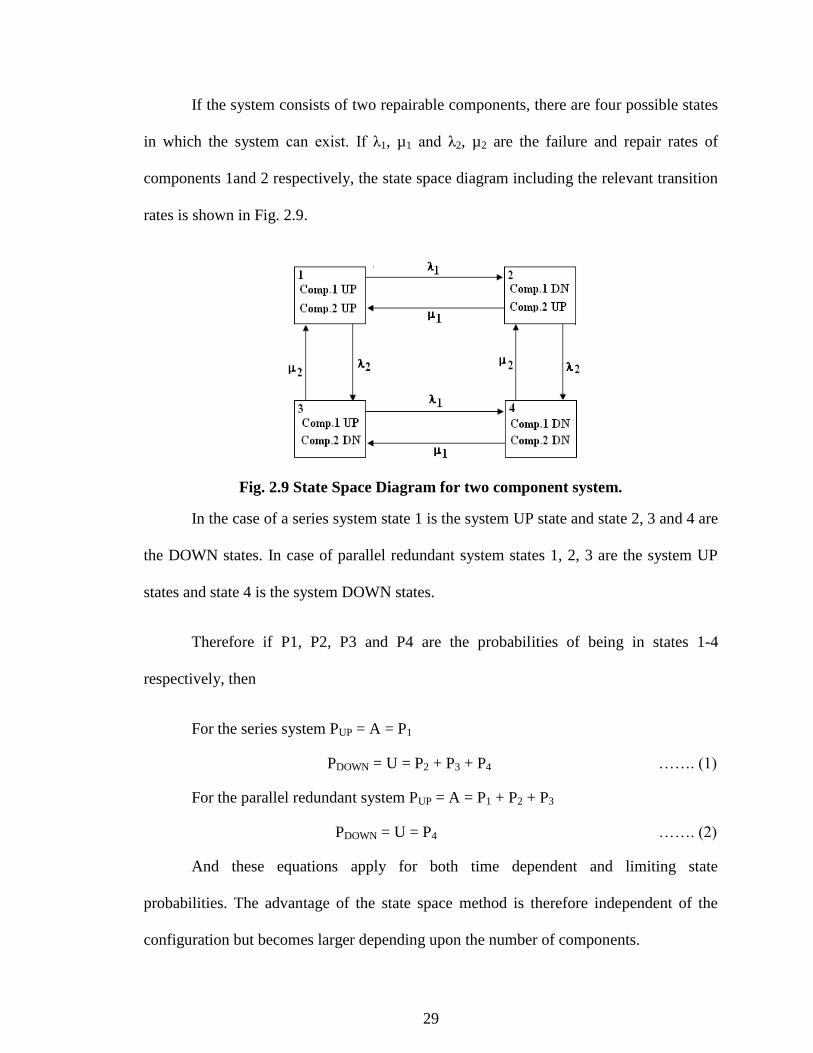
If the system consists of two repairable components, there are four possible states

in which the system can exist. If λ1, µ1 and λ2, µ2 are the failure and repair rates of

components 1and 2 respectively, the state space diagram including the relevant transition

rates is shown in Fig. 2.9.

Fig. 2.9 State Space Diagram for two component system.

In the case of a series system state 1 is the system UP state and state 2, 3 and 4 are

the DOWN states. In case of parallel redundant system states 1, 2, 3 are the system UP

states and state 4 is the system DOWN states.

Therefore if P1, P2, P3 and P4 are the probabilities of being in states 1-4

respectively, then

For the series system PUP = A = P1

PDOWN = U = P2 + P3 + P4 ……. (1)

For the parallel redundant system PUP = A = P1 + P2 + P3

PDOWN = U = P4 ……. (2)

And these equations apply for both time dependent and limiting state

probabilities. The advantage of the state space method is therefore independent of the

configuration but becomes larger depending upon the number of components.

30

Each state is shown by a rectangle in which the enclosed left side numbers are

associated respectively with the state number. The capacities associated with state 2 to 16

are proportional to the number of the available modules. The emergency state or spare

state, state 17 and 18, is a transition state between states1, 2, 3, 4, 5, 6, 7, 8, 9, 10, 11, 12,

13, 14, 15, 16 and state 19.

Fig. 2.10: RLD for combination of TCSC and Series Compensator using State –

Space Representation

31

From the above reliability logic diagram, matrix P, which is a Stochastic

Transitional Probability Matrix (STPM) is defined as:

16100

100000000000000000

010000000000000000

000210000000000000

000)

2(1000000000000

0000)

2(100000000000

00000)

(100000000000

000000)

2(1000000000

0000)4

2(100000000

00000)4

2(10000000

0000000)3

(10000000

0000000000)

2(100000

00000000)4

2(10000

000000000)4

2(1000

00000000000)3

(1000

00000000000000)

(100

0000000000000)3

(10

00000000000000)3

(1000000000000000021

P

SSSS PPP

Where, PSS = [P1 P2 P3 ……………… P17 P18 P19] which is a limiting state probability vector.

The following equations are developed from the expression SSSS PPP . The

above expression is derived by multiplying with PSS which is a limiting state probability

vector both sides of STPM (Stochastic Transitional Probability Matrix).

Expressing the above matrix form in terms of equations,

119521 PPPP)21(P . . . (2.5)

2196321 PPPP))3(1(PP . . . (2.6)

32

3197432 PPPP))3(1(PP . . . (2.7)

419843 PPP))(1(PP . . . (2.8)

5199651 PPPP))3(1(PP . . . (2.9)

619107652 PPPP))42(1(PPP . . . (2.10)

719118763 PPPP))42(1(PPP . . . (2.11)

81912874 PPP))2(1(PPP . . . (2.12)

919131095 PPPP))3(1(PP . . . (2.13)

101914111096 PPPP))42(1(PPP . . . (2.14)

1119151211107 PPPP))42(1(PPP . . . (2.15)

12191612118 PPP))2(1(PPP . . . (2.16)

131914139 PPP))(1(PP . . . (2.17)

141915141310 PPP))2(1(PPP . . . (2.18)

151916151411 PPP))2(1(PPP . . . (2.19)

1619161512 PP)21(PPP . . . (2.20)

171711109765 P)1(PPPPPPP . . . (2.21)

181811107632 P)1(PPPPPPP . . . (2.22)

19191817 P)161(PPP . . . (2.23)

Since all the above Eqns. (2.5 to 2.23) are independent to each other, we consider

only 18 equations out of the above 19 equations and 19th

equation is taken as

P1+P2+P3+P4+………………..+P17+P18+P19 = 1 . . . (2.24)

33

Writing the above Eqns. (2.4 to 2.22) and (2.24) in matrix form,

1

0

0

0

0

0

0

0

0

0

0

0

0

0

0

0

0

0

0

P

P

P

P

P

P

P

P

P

P

P

P

P

P

P

P

P

P

P

1111111111111111111

000000000000

000000000000

0020000000000000

00)

2(000000000000

000)

2(00000000000

0000)

(00000000000

00000)

2(000000000

00000)4

2(00000000

000000)4

2(0000000

0000000)3

(0000000

000000000)

2(00000

000000000)4

2(0000

0000000000)4

2(000

00000000000)3

(000

0000000000000)

(00

0000000000000)3

(0

00000000000000)3

(0000000000000002

19

18

17

16

15

14

13

12

11

10

9

8

7

6

5

4

3

2

1

. . . (2.25)

2.4.1 Results

From the above matrix form (Eqn. 2.25), find the limiting state probabilities.

Consider the data: Failure Rate (λ) = 0.7 f/yr

Repair Rate (μ) = 150 hrs of each component, then

Individual Limiting State Probabilities are:

P1 = 0.9814 P2 = 0.0046 P3 = 0.00025 P4 = 1.2 e-4

P5 = 2.3 e-5

P6 = 11.2 e-6 P7 = 23.2 e-6

P8 = 13.2 e-7

P9 = 43.8 e-8 P10 = 47.8 e-8

P11 = 12.8 e-9

P12 =53.2 e-10

P13 = 12.6 e-11

P14 = 11.8 e-12

P15 = 14.7 e-13 P16 =12.3 e-14

P17 = 0.0068 P18 = 0.0068 P19 = 27.3 e-6

Therefore, the sum of the limiting state probabilities is

34

P1+P2+P3+P4+P5+P6+P7+P8+P9+P10+P11+P12+P13+P14+P15+P16+P17+P18+P19 = 1

Availability of the system (PUP) = P1+P17+P18 = 0.9814 + 0.0068 + 0.0068 = 0.995

Unavailability (PDOWN) = 1-0.995 = 0.005

2.5 Load Indices

Reliability analysis of the entire transmission system is being carried out by using

load indices [61] like Loss of Load Expectation (LOLE) and Loss of Energy Expectation

(LOEE) [11].

The variations in the LOEE and LOLE [8] with system peak load are shown in

Figs. 2.11 & 2.12 respectively. The annual load factor is assumed to be 70%. It can be

seen that, for a give peak load, the LOEE and LOLE decrease with the employment of the

TCSC. The inclusion of the TCSC allows the capacity of transmission line to be extended

to its thermal limit and therefore, transfer more available capacity from the remote

generation site to the load point. The inclusion of series compensator allows reducing the

effect of inductance.

2.5.1 Calculations for LOEE:

LOEE (Loss of Energy Expectation) is the expected energy that will not be supplied due

to those occasions when the load demand exceeds the available capacity. The

probabilities of having varying amounts of capacity unavailable are combined with the

system load. Any outage of generating capacity exceeding the reserve will result in a

curtailment of system load energy.

n

1ikkPELOEE ……. (3)

Where Ok = Magnitude of the Capacity Outage

Pk = Probability of a Capacity Outage equal to Ok

35

Ek = Energy Curtailed by a capacity outage equal to Ok

The probable energy curtailed is EkPk. The sum of these products is the total

expected energy curtailment or loss of energy expectation (LOEE).

For Remote Generation, U = 0.01 & A = 0.99

Table 2.3: EENS for Remote Generation

Capacity out

of Service

Capacity in

Service Probability

0

735

1470

2205

2940

3675

4410

5145

5880

5880

5145

4410

3675

2940

2205

1470

735

0

0.922

0.07456

2.6348*10-3

5.325*10-5

6.7235*10-7

5.43312*10-9

2.74428*10-11

7.92*10-14

1*10-6

36

Individual probabilities can be found using the relation nCr R

n-r Q

r

From the Fig. tan θ = (5145 – 2940) / 100 = 22.05, θ = tan-1

(22.05) = 87.403

Total energy curtailed = Total area of curve

= Area of OACF + Area of ACB

= 2940*100 + 0.5 * 100 * 2205 = 404.25 GW

For 735 MW capacity outage = 0.5 * 4410 * 200 = 441 GW = 10.451 GW hr/yr

Therefore, the expected energy not supplied for remote generation is:

EENS (GW hr) = 10.451 + 3.6 + 1.5 + 1.0 + 0.85 = 17.401 GW hr/yr

For Local Generation (1),

Table 2.4: EENS for Local Generation (1)

Capacity out

of Service

Capacity in

Service Probability

0

1030

2060

2060

1030

0

0.9801

0.0198

0.0001

Therefore, the expected energy not supplied for local generation (1) is:

EENS (GW hr) = 3.97 + 2.11 + 0.89 = 6.97 GW hr/yr

For Local Generation (2),

Table 2.5: EENS for Local Generation (2)

Capacity out

of Service

Capacity in

Service Probability

0

280

560

560

280

0

0.9801

0.0198

0.0001

37

Therefore, the expected energy not supplied for Local Generation is:

EENS (GW hr) = 2.1 + 1.2 + 0.7 = 4.0 GW hr/yr

Total EENS (Local (1 & 2) + Generation) = 17.401 + 6.97 + 4.0

= 28.371 GW hr/yr

Fig. 2.11: Peak Load (MW) vs LOEE (GWhr/yr) wrt TCSC

Addition of capacitance in series with the transmission line modifies the reactance

of the line. The difference is very small for lower system peak loads, as the local

generation has sufficient capacity to prevent load interruption. The TCSC effect becomes

significant as the peak load increases.

2.5.2 Calculations for LOLE:

Peak Load is considered as 8500 MW, Number of occurrence is 12, 83, 107, 116

and 47 for peak loads of 7940, 7470, 6910, 6440 and 5145 respectively for individual

probability of capacity in service.

38

Table 2.6: Data for Generation System

Generation No. of

Units

Capacity

[MW]

Remote 8 735

Local

2 1030

2 280

Total capacity = 8*735 + 2*1030 + 2*280 = 5880 + 2060 + 560 = 8500MW

Failure rate (λ) = 0.01, Repair rate (μ) = 0.49

Availability (A) = 0.49 / (0.01+0.49) = 0.98

Unavailability (U) = 1 - 0.98 = 0.02

Individual probabilities can be found using the relation nCr R

r Q

n-r

Table 2.7: Individual Probabilities for Loss of Load Occurrence

Capacity Out

of Service

Capacity in

Service

Individual

Probability

0

560

1030

1590

2060

2620

3355

4825

5560

6295

7030

7765

8500

8500

7940

7470

6910

6440

5880

5145

3675

2940

2205

1470

735

0

0.7847

0.192

0.0215

1.466*10-3

6.732*10-5

2.1998*10-6

5.238*10-8

9.163*10-10

1.1687*10-11

1.06*10-13

6.49*10-16

2.408*10-18

4.096*10-21

39

LOLE = 12 Pi (8500-7940) + 83 Pi (8500-7470) + 107 Pi (8500-6910) + 116 Pi (8500-

6440) + 47 Pi (8500-5145)

= 12 Pi 560 + 83 Pi 1030 + 107 Pi 1590+ 116 Pi 2060 + 47 Pi 3355

= 12*0.192 + 83*0.0215 + 107*1.46*10-3

+ 116*6.732*10-5

+ 47*5.23*10-8

= 4.252 days / yr = 102 hr / yr

LOLE is computed for the system shown in Fig. 2.1. LOLE is computed using the

relation n

1i

iii )LC(PLOLE days/period. The system load factor is varied from 50 to

100% in steps of 5% for the analysis.

Fig. 2.12: Peak Load (MW) vs LOLE (hr/yr) wrt TCSC

Fig. 2.11 & 2.12 shows the variation in LOLE & LOEE with respect to system

peak load respectively. The annual load factor is assumed to be 70%. It can be seen that,

for a given peak load, the LOLE & LOEE decreases with the employment of TCSC &

Series Compensator. The inclusion of TCSC & Series compensator allows the capacity of

40

transmission line L1 to be extended to its thermal limits and therefore transfer more

available capacity from the remote generation site to the load point. The difference is

very small for lower system peak loads, as the local generation has sufficient capacity to

prevent load interruption. The TCSC effect becomes significant as the peak load

increases.

The impact of TCSC and series compensator on the LOEE and LOLE [8] are

shown in Figs. 2.13 & 2.14 respectively. The system load factor is varied from 50% to

100% in steps of 5%. It can be seen from these Figs. 2.13 & 2.14 that the LOEE and

LOLE increases with the system load factor.

Fig. 2.13: Load Factor (%) vs LOEE (GW hr/yr) wrt TCSC

41

Fig. 2.14: Load Factor (%) vs LOLE (hr/yr) wrt TCSC

Fig. 2.13 & 2.14 shows the impact of the TCSC & series compensator on LOLE

& LOEE when the annual system peak load is assumed to be 8500MW respectively. The

system load factor is varied from 50 to 100% in steps of 5%. It can be seen from the

figures that LOLE & LOEE increases with increase in the system load factor. It can be

seen that for a given load factor, the system reliability is considerably improved by the

inclusion of TCSC & Series Compensator.

The results are tabulated in Table 2.8 to 2.11 for different factors for constant

system peak load. It can be seen from table that for a given load factor, the system

reliability is considerably improved by the inclusion of TCSC and series compensator.

Tables 2.8 to 2.11 are developed for the system which is shown in Fig. 2.1.

42

Table 2.8: Load (MW) vs LOLE (hr/yr) wrt TCSC

LOLE

Load MW without TCSC with TCSC TCSC & SC

7800 15 2 1.8

8100 22 3 2.7

8400 65 8 7.1

8500 101 13 10.7

8700 204 23 19.4

9000 523 54 47.5

Table 2.9: Load (MW) vs LOEE (GW hr/yr) wrt TCSC

LOEE

Load MW without TCSC with TCSC TCSC & SC

7500 2 0.1 0

7800 5 0.7 0.52

8100 11.346 1.8 1.3

8400 24.268 3.92 2.97

8500 27.974 5.86 4.17

8700 52.131 10.92 8.62

9000 154.231 23.261 20.16

Table 2.10: Load Factor vs LOLE (hr/yr) wrt TCSC

LOLE

Load Factor without TCSC with TCSC TCSC & SC

50 60 7 5.8

60 83 8 6.2

70 101 13 11.7

80 198 19 16.1

90 303 38 33.4

95 401 46 39.2

43

Table 2.11: Load Factor vs LOEE (GW hr/yr) wrt TCSC

LOEE

Load Factor without TCSC with TCSC TCSC & SC

50 18.241 3.624 3.217

60 20.912 4.138 3.838

70 27.974 5.86 5.127

80 41.215 9.631 8.313

90 83.809 17.48 16.006

95 103.713 26.416 24.318

From Tables 2.8 and 2.9 it can be observed that, for any load LOLE & LOEE is

decreasing for different configurations viz. without TCSC, with TCSC and TCSC &

Series Compensator, which indicates that the combination TCSC & SC is preferable for

reduction of losses either in load or in energy indices. Similarly from Tables 2.10 and

2.11, instead of load (MW) load factor of the system is considered to prove the reduction

in losses.

2.6 Conclusions

In this chapter, reliability analysis of TCSC and series compensator is estimated

with deterministic probability values with the available component data. Further, an

attempt also has been made to estimate the availability of the combination of TCSC and

series compensator using time dependant probabilities. These time dependant

probabilities assume exponential distribution of the failure of the components where as

the deterministic probability data is based on binomial distribution. Load indices are also

calculated using load factor & system load for the sample Power Systems Network.