chapter 2 renewal-reward processes - pudn.comread.pudn.com/downloads74/ebook/272070/a first course...

CHAPTER 2

Renewal-Reward Processes

2.0 INTRODUCTION

The renewal-reward model is an extremely useful tool in the analysis of appliedprobability models for inventory, queueing and reliability applications, among oth-ers. Many stochastic processes are regenerative; that is, they regenerate themselvesfrom time to time so that the behaviour of the process after the regeneration epochis a probabilistic replica of the behaviour of the process starting at time zero. Thetime interval between two regeneration epochs is called a cycle. The sequence ofregeneration cycles constitutes a so-called renewal process. The long-run behaviourof a regenerative stochastic process on which a reward structure is imposed canbe studied in terms of the behaviour of the process during a single regenerationcycle. The simple and intuitively appealing renewal-reward model has numerousapplications.

In Section 2.1 we first discuss some elementary results from renewal theory. Amore detailed treatment of renewal theory will be given in Chapter 8. Section 2.2deals with the renewal-reward model. It shows how to calculate long-run aver-ages such as the long-run average reward per time unit and the long-run fractionof time the system spends in a given set of states. Illustrative examples will begiven. Section 2.3 discusses the formula of Little. This formula is a kind of lawof nature and relates among others the average queue size to the average wait-ing time in queueing systems. Another fundamental result that is frequently usedin queueing and inventory applications is the property that Poisson arrivals seetime averages (PASTA). This result is discussed in some detail in Section 2.4. ThePASTA property is used in Section 2.5 to obtain the famous Pollaczek–Khintchineformula from queueing theory. The renewal-reward model is used in Section 2.6 toobtain a generalization of the Pollaczek–Khintchine formula in the framework ofa controlled queue. Section 2.7 shows how renewal theory and an up- and down-crossing argument can be combined to derive a relation between time-average andcustomer-average probabilities in queues.

A First Course in Stochastic Models H.C. Tijmsc© 2003 John Wiley & Sons, Ltd. ISBNs: 0-471-49880-7 (HB); 0-471-49881-5 (PB)

34 RENEWAL-REWARD PROCESSES

2.1 RENEWAL THEORY

As a generalization of the Poisson process, renewal theory concerns the study ofstochastic processes counting the number of events that take place as a functionof time. Here the interoccurrence times between successive events are indepen-dent and identically distributed random variables. For instance, the events couldbe the arrival of customers to a waiting line or the successive replacements oflight bulbs. Although renewal theory originated from the analysis of replacementproblems for components such as light bulbs, the theory has many applications toquite a wide range of practical probability problems. In inventory, queueing andreliability problems, the analysis is often based on an appropriate identification ofembedded renewal processes for the specific problem considered. For example, ina queueing process the embedded events could be the arrival of customers whofind the system empty, or in an inventory process the embedded events could bethe replenishment of stock when the inventory position drops to the reorder pointor below it.

Formally, let X1, X2, . . . be a sequence of non-negative, independent randomvariables having a common probability distribution function

F(x) = P {Xk ≤ x}, x ≥ 0

for k = 1, 2, . . . . Letting µ1 = E(Xk), it is assumed that

0 < µ1 < ∞.

The random variable Xn denotes the interoccurrence time between the (n − 1)thand nth event in some specific probability problem. Define

S0 = 0 and Sn =n∑

i=1

Xi, n = 1, 2, . . . .

Then Sn is the epoch at which the nth event occurs. For each t ≥ 0, let

N(t) = the largest integer n ≥ 0 for which Sn ≤ t.

Then the random variable N(t) represents the number of events up to time t .

Definition 2.1.1 The counting process {N(t), t ≥ 0} is called the renewal processgenerated by the interoccurrence times X1, X2, . . . .

It is said that a renewal occurs at time t if Sn = t for some n. For each t ≥ 0, thenumber of renewals up to time t is finite with probability 1. This is an immediateconsequence of the strong law of large numbers stating that Sn/n → E(X1) withprobability 1 as n → ∞ and thus Sn ≤ t only for finitely many n. The Poissonprocess is a special case of a renewal process. Here we give some other examplesof a renewal process.

RENEWAL THEORY 35

Example 2.1.1 A replacement problem

Suppose we have an infinite supply of electric bulbs, where the burning times ofthe bulbs are independent and identically distributed random variables. If the bulbin use fails, it is immediately replaced by a new bulb. Let Xi be the burning time ofthe ith bulb, i = 1, 2, . . . . Then N(t) is the total number of bulbs to be replacedup to time t .

Example 2.1.2 An inventory problem

Consider a periodic-review inventory system for which the demands for a singleproduct in the successive weeks t = 1, 2, . . . are independent random variableshaving a common continuous distribution. Let Xi be the demand in the ith week,i = 1, 2, . . . . Then 1+N(u) is the number of weeks until depletion of the currentstock u.

2.1.1 The Renewal Function

An important role in renewal theory is played by the renewal function M(t) whichis defined by

M(t) = E[N(t)], t ≥ 0. (2.1.1)

For n = 1, 2, . . . , define the probability distribution function

Fn(t) = P {Sn ≤ t}, t ≥ 0.

Note that F1(t) = F(t). A basic relation is

N(t) ≥ n if and only if Sn ≤ t. (2.1.2)

This relation implies that

P {N(t) ≥ n} = Fn(t), n = 1, 2, . . . . (2.1.3)

Lemma 2.1.1 For any t ≥ 0,

M(t) =∞∑

n=1

Fn(t). (2.1.4)

Proof Since for any non-negative integer-valued random variable N ,

E(N) =∞∑

k=0

P {N > k} =∞∑

n=1

P {N ≥ n},

the relation (2.1.4) is an immediate consequence of (2.1.3).


In Exercise 2.4 the reader is asked to prove that M(t) < ∞ for all t ≥ 0. InChapter 8 we will discuss how to compute the renewal function M(t) in general.The infinite series (2.1.4) is in general not useful for computational purposes. Anexception is the case in which the interoccurrence times X1, X2, . . . have a gammadistribution with shape parameter α > 0 and scale parameter λ > 0. Then the sumX1+· · ·+Xn has a gamma distribution with shape parameter nα and scale parameterλ. In this case Fn(t) is the so-called incomplete gamma integral for which efficientnumerical procedures are available; see Appendix B. Let us explain this in moredetail for the case that α is a positive integer r so that the interoccurrence timesX1, X2, . . . have an Erlang (r, λ) distribution with scale parameter λ. Then Fn(t)

becomes the Erlang (nr, λ) distribution function

Fn(t) = 1 −nr−1∑k=0

e−λt (λt)k

k!, t ≥ 0

and thus

M(t) =∞∑

n=1

[1 −

nr−1∑k=0

e−λt (λt)k

k!

], t ≥ 0. (2.1.5)

In this particular case M(t) can be efficiently computed from a rapidly converg-ing series. For the special case that the interoccurrence times are exponentiallydistributed (r = 1), the expression (2.1.5) reduces to the explicit formula

M(t) = λt, t ≥ 0.

This finding is in agreement with earlier results for the Poisson process.

Remark 2.1.1 The phase methodA very useful interpretation of the renewal process {N(t)} can be given when theinteroccurrence times X1, X2, . . . have an Erlang distribution. Imagine that tokensarrive according to a Poisson process with rate λ and that the arrival of each rthtoken triggers the occurrence of an event. Then the events occur according to arenewal process in which the interoccurrence times have an Erlang (r, λ) distri-bution with scale parameter λ. The explanation is that the sum of r independent,exponentially distributed random variables with the same scale parameter λ has anErlang (r, λ) distribution. The phase method enables us to give a tractable expres-sion of the probability distribution of N(t) when the interoccurrence times have anErlang (r, λ) distribution. In this case P {N(t) ≥ n} is equal to the probability thatnr or more arrivals occur in a Poisson arrival process with rate λ. You are askedto work out the equivalence in Exercise 2.5.

Asymptotic expansion

A very useful asymptotic expansion for the renewal function M(t) can be givenunder a weak regularity condition on the interoccurrence times. This condition

RENEWAL THEORY 37

will be formulated in Section 8.2. For the moment it is sufficient to assume thatthe interoccurrence times have a positive density on some interval. Further it isassumed that µ2 = E(X2

1) is finite. Then it will be shown in Theorem 8.2.3 that

limt→∞

[M(t) − t

µ1

]= µ2

2µ21

− 1. (2.1.6)

The approximation

M(t) ≈ t

µ1+ µ2

2µ21

− 1 for t large

is practically useful for already moderate values of t provided that the squaredcoefficient of variation of the interoccurrence times is not too large and not tooclose to zero.

2.1.2 The Excess Variable

In many practical probability problems an important quantity is the random variableγt defined as the time elapsed from epoch t until the next renewal after epoch t .More precisely, γt is defined as

γt = SN(t)+1 − t ;

see also Figure 2.1.1 in which a renewal epoch is denoted by ×. Note that SN(t)+1is the epoch of the first renewal that occurs after time t . The random variableγt is called the excess or residual life at time t . For the replacement problem ofExample 2.1.1 the random variable γt denotes the residual lifetime of the light bulbin use at time t .

Lemma 2.1.2 For any t ≥ 0,

E(γt ) = µ1[1 + M(t)] − t. (2.1.7)

Proof Fix t ≥ 0. To prove (2.1.7), we apply Wald’s equation from Appendix A.To do so, note that N(t) ≤ n − 1 if and only if X1 + · · · + Xn > t . Hence theevent {N(t) + 1 = n} depends only on X1, . . . , Xn and is thus independent ofXn+1, Xn+2, . . . . Hence

E

N(t)+1∑

k=1

Xk

= E(X1)E[N(t) + 1],

which gives (2.1.7).

0 S1 S2 tSN(t) SN(t) + 1 Time

gt

Figure 2.1.1 The excess life


In Corollary 8.2.4 it will be shown that

limt→∞ E(γt ) = µ2

2µ1and lim

t→∞ E(γ 2t ) = µ3

3µ1(2.1.8)

with µk = E(Xk1) for k = 1, 2, 3, provided that the interoccurrence times have a

positive density on some interval. An illustration of the usefulness of the conceptof excess variable is provided by the next example.

Example 2.1.3 The average order size in an (s, S) inventory system

Suppose a periodic-review inventory system for which the demands X1, X2, . . .

for a single product in the successive weeks 1, 2, . . . are independent randomvariables having a common probability density f (x) with finite mean α and finitestandard deviation σ . Any demand exceeding the current inventory is backloggeduntil inventory becomes available by the arrival of a replenishment order. Theinventory position is reviewed at the beginning of each week and is controlled byan (s, S) rule with 0 ≤ s < S. Under this control rule, a replenishment order ofsize S −x is placed when the review reveals that the inventory level x is below thereorder point s; otherwise, no ordering is done. We assume instantaneous deliveryof every replenishment order.

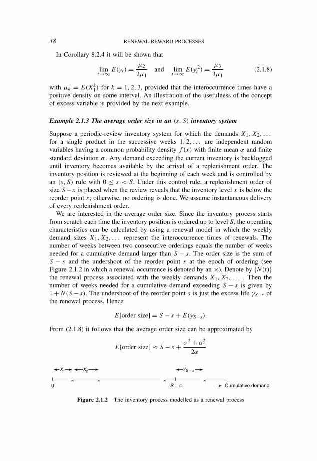
We are interested in the average order size. Since the inventory process startsfrom scratch each time the inventory position is ordered up to level S, the operatingcharacteristics can be calculated by using a renewal model in which the weeklydemand sizes X1, X2, . . . represent the interoccurrence times of renewals. Thenumber of weeks between two consecutive orderings equals the number of weeksneeded for a cumulative demand larger than S − s. The order size is the sum ofS − s and the undershoot of the reorder point s at the epoch of ordering (seeFigure 2.1.2 in which a renewal occurrence is denoted by an ×). Denote by {N(t)}the renewal process associated with the weekly demands X1, X2, . . . . Then thenumber of weeks needed for a cumulative demand exceeding S − s is given by1 + N(S − s). The undershoot of the reorder point s is just the excess life γS−s ofthe renewal process. Hence

E[order size] = S − s + E(γS−s).

From (2.1.8) it follows that the average order size can be approximated by

E[order size] ≈ S − s + σ 2 + α2

2α

0 S − s Cumulative demand

gS − sX1 X2

Figure 2.1.2 The inventory process modelled as a renewal process

RENEWAL-REWARD PROCESSES 39

provided that S − s is sufficiently large compared with E(weekly demand). Inpractice this is a useful approximation for S−s > α when the weekly demand is nothighly variable and has a squared coefficient of variation between 0.2 and 1 (say).

Another illustration of the importance of the excess variable is given by thefamous waiting-time paradox.

Example 2.1.4 The waiting-time paradox

We have all experienced long waits at a bus stop when buses depart irregularly andwe arrive at the bus stop at random. A theoretical explanation of this phenomenon isprovided by the expression for limt→∞ E(γt ). Therefore it is convenient to rewrite(2.1.8) as

limt→∞ E(γt ) = 1

2(1 + c2

X)µ1, (2.1.9)

where

c2X = σ 2(X1)

E2(X1)

is the squared coefficient of variation of the interdeparture times X1, X2, . . . . Theequivalent expression (2.1.9) follows from (2.1.8) by noting that

1 + c2X = 1 + µ2 − µ2

1

µ21

= µ2

µ21

. (2.1.10)

The representation (2.1.9) makes clear that

limt→∞ E(γt ) =

{< µ1 if c2

X < 1,

> µ1 if c2X > 1.

Thus the mean waiting time for the next bus depends on the regularity of the busservice and increases with the coefficient of variation of the interdeparture times. Ifwe arrive at the bus stop at random, then for highly irregular service (c2

X > 1) themean waiting time for the next bus is even larger than the mean interdeparture time.This surprising result is sometimes called the waiting-time paradox. A heuristicexplanation is that it is more likely to hit a long interdeparture time than a shortone when arriving at the bus stop at random. To illustrate this, consider the extremesituation in which the interdeparture time is 0 minutes with probability 9/10 and is10 minutes with probability 1/10. Then the mean interdeparture time is 1 minute,but your mean waiting time for the next bus is 5 minutes when you arrive at thebus stop at random.

2.2 RENEWAL-REWARD PROCESSES

A powerful tool in the analysis of numerous applied probability models is therenewal-reward model. This model is also very useful for theoretical purposes. In


Chapters 3 and 4, ergodic theorems for Markov chains will be proved by usingthe renewal-reward theorem. The renewal-reward model is a simple and intuitivelyappealing model that deals with a so-called regenerative process on which a costor reward structure is imposed. Many stochastic processes have the property ofregenerating themselves at certain points in time so that the behaviour of the processafter the regeneration epoch is a probabilistic replica of the behaviour starting attime zero and is independent of the behaviour before the regeneration epoch.

A formal definition of a regenerative process is as follows.

Definition 2.2.1 A stochastic process {X(t), t ∈ T } with time-index set T is saidto be regenerative if there exists a (random) epoch S1 such that:

(a) {X(t + S1), t ∈ T } is independent of {X(t), 0 ≤ t < S1},(b) {X(t + S1), t ∈ T } has the same distribution as {X(t), t ∈ T }.

It is assumed that the index set T is either the interval T = [0, ∞) or the count-able set T = {0, 1, . . . }. In the former case we have a continuous-time regenerativeprocess and in the other case a discrete-time regenerative process. The state spaceof the process {X(t)} is assumed to be a subset of some Euclidean space.

The existence of the regeneration epoch S1 implies the existence of furtherregeneration epochs S2, S3, . . . having the same property as S1. Intuitively speak-ing, a regenerative process can be split into independent and identically distributedrenewal cycles. A cycle is defined as the time interval between two consecutiveregeneration epochs. Examples of regenerative processes are:

(i) The continuous-time process {X(t), t ≥ 0} with X(t) denoting the number ofcustomers present at time t in a single-server queue in which the customersarrive according to a renewal process and the service times are independentand identically distributed random variables. It is assumed that at epoch 0 acustomer arrives at an empty system. The regeneration epochs S1, S2, . . . arethe epochs at which an arriving customer finds the system empty.

(ii) The discrete-time process {In, n = 0, 1, . . . } with In denoting the inventorylevel at the beginning of the nth week in the (s, S) inventory model dealt within Example 2.1.3. Assume that the inventory level equals S at epoch 0. Theregeneration epochs are the beginnings of the weeks in which the inventorylevel is ordered up to the level S.

Let us define the random variables Cn = Sn −Sn−1, n = 1, 2, . . . , where S0 = 0by convention. The random variables C1, C2, . . . are independent and identicallydistributed. In fact the sequence {C1, C2, . . . } underlies a renewal process in whichthe events are the occurrences of the regeneration epochs. Hence we can interpretCn as

Cn = the length of the nth renewal cycle, n = 1, 2, . . . .


Note that the cycle length Cn assumes values from the index set T . In the followingit is assumed that

0 < E(C1) < ∞.

In many practical situations a reward structure is imposed on the regenerativeprocess {X(t), t ∈ T }. The reward structure usually consists of reward rates thatare earned continuously over time and lump rewards that are only earned at certainstate transitions. Let

Rn = the total reward earned in the nth renewal cycle, n = 1, 2, . . . .

It is assumed that R1, R2, . . . are independent and identically distributed randomvariables. In applications Rn typically depends on Cn. In case Rn can take on bothpositive and negative values, it is assumed that E(|R1|) < ∞. Let

R(t) = the cumulative reward earned up to time t.

The process {R(t), t ≥ 0} is called a renewal-reward process. We are now readyto prove a theorem of utmost importance.

Theorem 2.2.1 (renewal-reward theorem)

limt→∞

R(t)

t= E(R1)

E(C1)with probability 1.

In other words, for almost any realization of the process, the long-run averagereward per time unit is equal to the expected reward earned during one cycle dividedby the expected length of one cycle.

To prove this theorem we first establish the following lemma.

Lemma 2.2.2 For any t ≥ 0, let N(t) be the number of cycles completed up totime t . Then

limt→∞

N(t)

t= 1

E(C1)with probability 1.

Proof By the definition of N(t), we have

C1 + · · · + CN(t) ≤ t < C1 + · · · + CN(t)+1.

Since P {C1 + · · · + Cn < ∞} = 1 for all n ≥ 1, it is not difficult to verify that

limt→∞ N(t) = ∞ with probability 1.

The above inequality gives

C1 + · · · + CN(t)

N(t)≤ t

N(t)<

C1 + · · · + CN(t)+1

N(t) + 1

N(t) + 1

N(t).


By the strong law of large numbers for a sequence of independent and identicallydistributed random variables, we have

limn→∞

C1 + · · · + Cn

n= E(C1) with probability 1.

Hence, by letting t → ∞ in the above inequality, the desired result follows.

Lemma 2.2.2 is also valid when E(C1) = ∞ provided that P {C1 < ∞} = 1. Thereason is that the strong law of large numbers for a sequence {Cn} of non-negativerandom variables does not require that E(C1) < ∞. Next we prove Theorem 2.2.1.

Proof of Theorem 2.2.1 For ease, let us first assume that the rewards are non-negative. Then, for any t > 0,

N(t)∑i=1

Ri ≤ R(t) ≤N(t)+1∑

i=1

Ri.

This gives

N(t)∑i=1

Ri

N(t)× N(t)

t≤ R(t)

t≤

N(t)+1∑i=1

Ri

N(t) + 1× N(t) + 1

t.

By the strong law of large numbers for the sequence {Rn}, we have

limn→∞

1

n

n∑i=1

Ri = E(R1) with probability 1.

As pointed out in the proof of Lemma 2.2.2, N(t) → ∞ with probability 1 ast → ∞. Letting t → ∞ in the above inequality and using Lemma 2.2.2, the desiredresult next follows for the case that the rewards are non-negative. If the rewards canassume both positive and negative values, then the theorem is proved by treatingthe positive and negative parts of the rewards separately. We omit the details.

In a natural way Theorem 2.2.1 relates the behaviour of the renewal-rewardprocess over time to the behaviour of the process over a single renewal cycle. It isnoteworthy that the outcome of the long-run average actual reward per time unitcan be predicted with probability 1. If we are going to run the process over aninfinitely long period of time, then we can say beforehand that in the long run theaverage actual reward per time unit will be equal to the constant E(R1)/E(C1) withprobability 1. This is a much stronger and more useful statement than the statementthat the long-run expected average reward per time unit equals E(R1)/E(C1) (itindeed holds that limt→∞ E[R(t)]/t = E(R1)/E(C1); this expected-value versionof the renewal-reward theorem is a direct consequence of Theorem 2.2.1 whenR(t)/t is bounded in t but otherwise requires a hard proof). Also it is noted that forthe case of non-negative rewards Rn the renewal-reward theorem is also valid whenE(R1) = ∞ (the assumption E(C1) < ∞ cannot be dropped for Theorem 2.2.1).


Example 2.2.1 Alternating up- and downtimes

Suppose a machine is alternately up and down. Denote by U1, U2, . . . the lengthsof the successive up-periods and by D1, D2, . . . the lengths of the successivedown-periods. It is assumed that both {Un} and {Dn} are sequences of independentand identically distributed random variables with finite positive expectations. Thesequences {Un} and {Dn} are not required to be independent of each other. Assumethat an up-period starts at epoch 0. What is the long-run fraction of time the machineis down? The answer is

the long-run fraction of time the machine is down

= E(D1)

E(U1) + E(D1)with probability 1. (2.2.1)

To verify this, define the continuous-time stochastic process {X(t), t ≥ 0} by

X(t) ={

1 if the machine is up at time t,

0 otherwise.

The process {X(t)} is a regenerative process. The epochs at which an up-periodstarts can be taken as regeneration epochs. The long-run fraction of time themachine is down can be interpreted as a long-run average cost per time unitby assuming that a cost at rate 1 is incurred while the machine is down anda cost at rate 0 otherwise. A regeneration cycle consists of an up-period and adown-period. Hence

E(length of one cycle) = E(U1 + D1)

and

E(cost incurred during one cycle) = E(D1).

By applying the renewal-reward theorem, it follows that the long-run average costper time unit equals E(D1)/[E(U1) + E(D1)], proving the result (2.2.1).

The intermediate step of interpreting the long-run fraction of time that the processis in a certain state as a long-run average cost (reward) per time unit is very helpfulin many situations.

Limit theorems for regenerative processes

An important application of the renewal-reward theorem is the characterizationof the long-run fraction of time a regenerative process {X(t), t ∈ T } spends insome given set B of states. For the set B of states, define for any t ∈ T theindicator variable

IB(t) ={

1 if X(t) ∈ B,

0 if X(t) /∈ B.


Also, define the random variable

TB = the amount of time the process spends in the set B of states duringone cycle.

Note that TB = ∫ S10 IB(u) du for a continuous-time process {X(t)}; otherwise, TB

equals the number of indices 0 ≤ k < S1 with X(k) ∈ B. The following theoremis an immediate consequence of the renewal-reward theorem.

Theorem 2.2.3 For the regenerative process {X(t)} it holds that the long-runfraction of time the process spends in the set B of states is E(TB)/E(C1) withprobability 1.

That is,

limt→∞

1

t

∫ t

0IB(u) du = E(TB)

E(C1)with probability 1

for a continuous-time process {X(t)} and

limn→∞

1

n

n∑k=0

IB(k) = E(TB)

E(C1)with probability 1

for a discrete-time process {X(n)}.Proof The long-run fraction of time the process {X(t)} spends in the set B ofstates can be interpreted as a long-run average reward per time unit by assumingthat a reward at rate 1 is earned while the process is in the set B and a reward atrate 0 is earned otherwise. Then

E(reward earned during one cycle) = E(TB).

The desired result next follows by applying the renewal-reward theorem.

Since E(IB(t)) = P {X(t) ∈ B}, we have as consequence of Theorem 2.2.3 andthe bounded convergence theorem that, for a continuous-time process,

limt→∞

1

t

∫ t

0P {X(u) ∈ B} du = E(TB)

E(C1).

Note that (1/t)∫ t

0 P {X(u) ∈ B} du can be interpreted as the probability that anoutside observer arriving at a randomly chosen point in (0, t) finds the process inthe set B.

In many situations the ratio E(TB)/E(C1) could be interpreted both as the long-run fraction of time the process {X(t)} spends in the set B of states and as theprobability of finding the process in the set B when the process has reached sta-tistical equilibrium. This raises the question whether limt→∞ P {X(t) ∈ B} alwaysexists. This ordinary limit need not always exist. A counterexample is provided by


periodic discrete-time Markov chains; see Chapter 3. For completeness we statethe following theorem.

Theorem 2.2.4 For the regenerative process {X(t), t ∈ T },

limt→∞ P {X(t) ∈ B} = E(TB)

E(C1)

provided that the probability distribution of the cycle length has a continuous partin the continuous-time case and is aperiodic in the discrete-time case.

A distribution function is said to have a continuous part if it has a positivedensity on some interval. A discrete distribution {aj , j = 0, 1, . . . } is said tobe aperiodic if the greatest common divisor of the indices j ≥ 1 for whichaj > 0 is equal to 1. The proof of Theorem 2.2.4 requires deep mathematicsand is beyond the scope of this book. The interested reader is referred to Miller(1972). It is remarkable that the proof of Theorem 2.2.3 for the time-average limitlimt→∞ (1/t)

∫ t

0 IB(u) du is much simpler than the proof of Theorem 2.2.4 forthe ordinary limit limt→∞ P {X(t) ∈ B}. This is all the more striking when wetake into account that the time-average limit is in general much more usefulfor practical purposes than the ordinary limit. Another advantage of the time-average limit is that it is easier to understand than the ordinary limit. In interpret-ing the ordinary limit one should be quite careful. The ordinary limit representsthe probability that an outside person will find the process in some state of theset B when inspecting the process at an arbitrary point in time after the processhas been in operation for a very long time. It is essential for this interpretationthat the outside person has no information about the past of the process wheninspecting the process. How much more concrete is the interpretation of the time-average limit as the long-run fraction of time the process will spend in the set B

of states!To illustrate Theorem 2.2.4, consider again Example 2.2.1. In this example we

analysed the long-run average behaviour of the regenerative process {X(t)}, whereX(t) = 1 if the machine is up at time t and X(t) = 0 otherwise. It was shown thatthe long-run fraction of time the machine is down equals E(D)/[E(U) + E(D)],where the random variables U and D denote the lengths of an up-period and adown-period. This result does not require any assumption about the shapes of theprobability distributions of U and D. However, some assumption is needed in orderto conclude that

limt→∞ P {the system is down at time t} = E(D)

E(U) + E(D). (2.2.2)

It is sufficient to assume that the distribution function of the length of an up-periodhas a positive density on some interval.

We state without proof a central limit theorem for the renewal-reward process.


Theorem 2.2.5 Assume that R(t) ≥ 0 with E(C21) < ∞ and E(R2

1) < ∞. Then

limt→∞ P

{R(t) − gt

ν√

t/µ1≤ x

}= 1√

2π

∫ x

−∞e− 1

2 y2dy, x ≥ 0,

where µ1 = E(C1), µ2 = E(C21), g = E(R1)/E(C1) and ν2 = E(R1 − gC1)

2.

A proof of this theorem can be found in Wolff (1989). In applying this theo-rem, the difficulty is usually to find the constant ν. In specific applications onemight use simulation to find ν. As a special case, Theorem 2.2.5 includes a centrallimit theorem for the renewal process {N(t)} studied in Section 2.1. Taking therewards Rn equal to 1 it follows that the renewal process {N(t)} is asymptoticallyN(t/µ1, σ 2t/µ3

1) distributed with σ 2 = µ2 − µ21.

Next we give two illustrative examples of the renewal-reward model.

Example 2.2.2 A stochastic clearing system

In a communication system messages requiring transmission arrive according toa Poisson process with rate λ. The messages are temporarily stored in a bufferhaving ample capacity. Every T time units, the buffer is cleared from all messagespresent. The buffer is empty at time t = 0. A fixed cost of K > 0 is incurred foreach clearing of the buffer. Also, for each message there is a holding cost of h > 0for each time unit the message has to wait in the buffer. What is the value of T

for which the long-run average cost per time unit is minimal?We first derive an expression for the average cost per time unit for a given

value of the control parameter T . To do so, observe that the stochastic processdescribing the number of messages in the system regenerates itself each time thebuffer is cleared from all messages present. This fact uses the lack of memory ofthe Poisson arrival process so that at any clearing epoch it is not relevant howlong ago the last message arrived. Taking a cycle as the time interval between twosuccessive clearings of the buffer, we have

the expected length of one cycle = T .

To specify the expected cost incurred during one cycle, we need an expression forthe total waiting time of all messages arriving during one cycle. It was shown inExample 1.1.4 that

E[total waiting time in (0, T )] = 1

2λT 2.

This gives

E[cost incurred during one cycle] = K + 1

2hλT 2.


Hence, by the renewal-reward theorem,

the long-run average cost per time unit = 1

T

(K + 1

2hλT 2

)

with probability 1. When K = 0 and h = 1, the system incurs a cost at rate j

whenever there are j messages in the buffer, in which case the average cost pertime unit gives the average number of messages in the buffer. Hence

the long-run average number of messages in the buffer = 1

2λT .

Putting the derivative of the cost function equal to 0, it follows that the long-runaverage cost is minimal for

T ∗ =√

2K

hλ.

Example 2.2.3 A reliability system with redundancies

An electronic system consists of a number of independent and identical compo-nents hooked up in parallel. The lifetime of each component has an exponentialdistribution with mean 1/µ. The system is operative only if m or more componentsare operating. The non-failed units remain in operation when the system as a wholeis in a non-operative state. The system availability is increased by periodic main-tenance and by putting r redundant components into operation in addition to theminimum number m of components required. Under the periodic maintenance thesystem is inspected every T time units, where at inspection the failed componentsare repaired. The repair time is negligible and each repaired component is againas good as new. The periodic inspections provide the only repair opportunities.The following costs are involved. For each component there is a depreciation costof I > 0 per time unit. A fixed cost of K > 0 is made for each inspection andthere is a repair cost of R > 0 for each failed component. How can we choosethe number r of redundant components and the time T between two consecutiveinspections such that the long-run average cost per time unit is minimal subject tothe requirement that the probability of system failure between two inspections isno more than a prespecified value α?

We first derive the performance measures for given values of the parameters r

and T . The stochastic process describing the number of operating components isregenerative. Using the lack of memory of the exponential lifetimes of the compo-nents, it follows that the process regenerates itself after each inspection. Taking acycle as the time interval between two inspections, we have

E(length of one cycle) = T .


Further, using the fact that a given component fails within a time T with probability1 − e−µT , it follows that

P {the system as a whole fails between two inspections}

=m+r∑

k=r+1

(m + r

k

)(1 − e−µT )ke−µT (m+r−k)

andE(number of components that fail between two inspections)

= (m + r)(1 − e−µT ).

Hence

E(total costs in one cycle) = (m + r)I × T + K + (m + r)(1 − e−µT )R.

This givesthe long-run average cost per time unit

= 1

T[(m + r)I × T + K + (m + r)(1 − e−µT )R]

with probability 1. The optimal values of the parameters r and T are found fromthe following minimization problem:

Minimize1

T[(m + r)I × T + K + (m + r)(1 − e−µT )R]

subject tom+r∑

k=r+1

(m + r

k

)(1 − e−µT )ke−µT (m+r−k) ≤ α.

Using the Lagrange method this problem can be numerically solved.

Rare events∗

In many applied probability problems one has to study rare events. For example,a rare event could be a system failure in reliability applications or buffer overflowin finite-buffer telecommunication problems. Under general conditions it holds thatthe time until the first occurrence of a rare event is approximately exponentiallydistributed. Loosely formulated, the following result holds. Let {X(t)} be a regen-erative process having a set B of (bad) states such that the probability q thatthe process visits the set B during a given cycle is very small. Denote by therandom variable U the time until the process visits the set B for the first time.Assuming that the cycle length has a finite and positive mean E(T ), it holds thatP {U > t} ≈ e−tq/E(T ) for t ≥ 0; see Keilson (1979) or Solovyez (1971) for

∗This section may be skipped at first reading.


a proof. The result that the time until the first occurrence of a rare event in aregenerative process is approximately exponentially distributed is very useful. Itgives not only quantitative insight, but it also implies that the computation of themean of the first-passage time suffices to get the whole distribution.

In the next example we obtain the above result by elementary arguments.

Example 2.2.4 A reliability problem with periodic inspections

High reliability of an electronic system is often achieved by employing redundantcomponents and having periodic inspections. Let us consider a reliability systemwith two identical units, where one unit is in full operation and the other unit is inwarm standby. The operating unit has a constant failure rate of λ0 and the unit instandby has a constant failure rate of λ1, where 0 ≤ λ1 < λ0. Upon failure of theoperating unit, the standby unit is put into full operation provided the standby is notin the failure state. Failed units are replaced only at the scheduled times T , 2T , . . .

when the system is inspected. The time to replace any failed unit is negligible.A system failure occurs if both units are down. It is assumed that (λ0 + λ1)T issufficiently small so that a system failure is a rare event. In designing highly reliablesystems a key measure of system performance is the probability distribution of thetime until the first system failure.

To find the distribution of the time until the first system failure, we first computethe probability q defined by

q = P {system failure occurs between two inspections}.

To do so, observe that a constant failure rate λ for the lifetime of a unit implies thatthe lifetime has an exponential distribution with mean 1/λ. Using the fact that theminimum of two independent exponentials with respective means 1/λ0 and 1/λ1is exponentially distributed with mean 1/(λ0 +λ1), we find by conditioning on theepoch of the first failure of a unit that

q =∫ T

0

{1 − e−λ0(T −x)

}(λ0 + λ1) e−(λ0+λ1)x dx

= 1 − (λ0 + λ1)

λ1e−λ0T + λ0

λ1e−(λ0+λ1)T .

Assuming that both units are in good condition at epoch 0, let

U = the time until the first system failure.

Since the process describing the state of the two units regenerates itself at eachinspection, it follows that

P {U > nT } = (1 − q)n, n = 0, 1, . . . .


Assuming that the failure probability q is close to 0, the approximations (1−q)n ≈1 − nq and e−nq ≈ 1 − nq apply. Thus we find that

P {U > t} ≈ e−tq/T , t ≥ 0.

In other words, the time until the first system failure is approximately exponentiallydistributed.

2.3 THE FORMULA OF LITTLE

To introduce the formula of Little, we consider first two illustrative examples. Inthe first example a hospital admits on average 25 new patients per day. A patientstays on average 3 days in the hospital. What is the average number of occupiedbeds? Let λ = 25 denote the average number of new patients who are admittedper day, W = 3 the average number of days a patient stays in the hospital and L

the average number of occupied beds. Then L = λW = 25 × 3 = 75 beds. In thesecond example a specialist shop sells on average 100 bottles of a famous Mexicanpremium beer per week. The shop has on average 250 bottles in inventory. What isthe average number of weeks that a bottle is kept in inventory? Let λ = 100 denotethe average demand per week, L = 250 the average number of bottles kept in stockand W the average number of weeks that a bottle is kept in stock. Then the answeris W = L/λ = 250/100 = 2.5 weeks. These examples illustrate Little’s formulaL = λW . The formula of Little is a ‘law of nature’ that applies to almost anytype of queueing system. It relates long-run averages such as the long-run averagenumber of customers in a queue (system) and the long-run average amount of timespent per customer in the queue (system). A queueing system is described by thearrival process of customers, the service facility and the service discipline, to namethe most important elements. In formulating the law of Little, there is no need tospecify those basic elements. For didactical reasons, however, it is convenient todistinguish between queueing systems with infinite queue capacity and queueingsystems with finite queue capacity.

Infinite-capacity queues

Consider a queueing system with infinite queue capacity, that is, every arrivingcustomer is allowed to wait until service can be provided. Define the followingrandom variables:

Lq(t) = the number of customers in the queue at time t

(excluding those in service),

L(t) = the number of customers in the system at time t

(including those in service),

THE FORMULA OF LITTLE 51

Dn = the amount of time spent by the nth customer in the queue(excluding service time),

Un = the amount of time spent by the nth customer in the system(including service time).

Let us assume that each of the stochastic processes {Lq(t)}, {L(t)}, {Dn} and {Un}is regenerative and has a cycle length with a finite expectation. Then there areconstants Lq , L, Wq and W such that the following limits exist and are equal tothe respective constants with probability 1:

limt→∞

1

t

∫ t

0Lq(u) du = Lq (the long-run average number in queue),

limt→∞

1

t

∫ t

0L(u) du = L (the long-run average number in system),

limn→∞

1

n

n∑k=1

Dk = Wq (the long-run average delay in queue per customer),

limn→∞

1

n

n∑k=1

Uk = W (the long-run average sojourn time per customer).

Now define the random variable

A(t) = the number of customers arrived by time t,

It is also assumed that, for some constant λ,

limt→∞

A(t)

t= λ with probability 1.

The constant λ gives the long-run average arrival rate of customers. The limitλ exists when customers arrive according to a renewal process (or batches ofcustomers arrive according to a renewal process with independent and identicallydistributed batch sizes).

The existence of the above limits is sufficient to prove the basic relations

Lq = λWq (2.3.1)

andL = λW (2.3.2)

These basic relations are the most familiar form of the formula of Little. The readeris referred to Stidham (1974) and Wolff (1989) for a rigorous proof of the formulaof Little. Here we will be content to demonstrate the plausibility of this result. The


formula of Little is easiest understood (and reconstructed) when imagining that eachcustomer pays money to the system manager according to some non-discriminationrule. Then it is intuitively obvious that

the long-run average reward per time unit earned by the system

= (the long-run average arrival rate of paying customers) (2.3.3)

× (the long-run average amount received per paying customer).

In regenerative queueing processes this relation can often be directly proved byusing the renewal-reward theorem; see Exercise 2.26. Taking the ‘money principle’(2.3.3) as starting point, it is easy to reproduce various representations of Little’slaw. To obtain (2.3.1), imagine that each customer pays $1 per time unit whilewaiting in queue. Then the long-run average amount received per customer equalsthe long-run average time in queue per customer (= Wq ). On the other hand, thesystem manager receives $j for each time unit that there are j customers waitingin queue. Hence the long-run average reward earned per time unit by the systemmanager equals the long-run average number of customers waiting in queue (= Lq).The average arrival rate of paying customers is obviously given by λ. Applying therelation (2.3.3) gives next the formula (2.3.1). The formula (2.3.2) can be seen bya very similar reasoning: imagine that each customer pays $1 per time unit whilein the system. Another interesting relation arises by imagining that each customerpays $1 per time unit while in service. Denoting by E(S) the long-run averageservice time per customer, it follows that

the long-run average number of customers in service = λE(S). (2.3.4)

If each customer requires only one server and each server can handle only onecustomer at a time, this relation leads to

the long-run average number of busy servers = λE(S). (2.3.5)

Finite-capacity queues

Assume now there is a maximum on the number of customers allowed in thesystem. In other words, there are only a finite number of waiting places and eacharriving customer finding all waiting places occupied is turned away. It is assumedthat a rejected customer has no further influence on the system. Let the rejectionprobability Prej be defined by

Prej = the long-run fraction of customers who are turned away,

assuming that this long-run fraction is well defined. The random variables L(t),Lq(t), Dn and Un are defined as before, except that Dn and Un now refer to thequeueing time and sojourn time of the nth accepted customer. The constants Wq

and W now represent the long-run average queueing time per accepted customer

POISSON ARRIVALS SEE TIME AVERAGES 53

and the long-run average sojourn time per accepted customer. The formulas (2.3.1),(2.3.2) and (2.3.4) need only slight modification:

Lq = λ(1 − Prej )Wq and L = λ(1 − Prej )W, (2.3.6)

the long-run average number of customers in service

= λ(1 − Prej )E(S). (2.3.7)

Heuristically, these formulas follow by applying the money principle (2.3.3) andtaking only the accepted customers as paying customers.

2.4 POISSON ARRIVALS SEE TIME AVERAGES

In the analysis of queueing (and other) problems, one sometimes needs the long-run fraction of time the system is in a given state and sometimes needs the long-run fraction of arrivals who find the system in a given state. These averages canoften be related to each other, but in general they are not equal to each other. Toillustrate that the two averages are in general not equal to each other, suppose thatcustomers arrive at a service facility according to a deterministic process in whichthe interarrival times are 1 minute. If the service of each customer is uniformlydistributed between 1

4 minute and 34 minute, then the long-run fraction of time the

system is empty equals 12 , whereas the long-run fraction of arrivals finding the

system empty equals 1. However the two averages would have been the same ifthe arrival process of customers had been a Poisson process. As a prelude to thegenerally valid property that Poisson arrivals see time averages, we first analysetwo specific problems by the renewal-reward theorem.

Example 2.4.1 A manufacturing problem

Suppose that jobs arrive at a workstation according to a Poisson process with rateλ. The workstation has no buffer to store temporarily arriving jobs. An arriving jobis accepted only when the workstation is idle, and is lost otherwise. The processingtimes of the jobs are independent random variables having a common probabilitydistribution with finite mean β. What is the long-run fraction of time the workstationis busy and what is the long-run fraction of jobs that are lost?

These two questions are easily answered by using the renewal-reward theorem.Let us define the following random variables. For any t ≥ 0, let

I (t) ={

1 if the workstation is busy at time t,

0 otherwise.

Also, for any n = 1, 2, . . . , let

In ={

1 if the workstation is busy just prior to the nth arrival,

0 otherwise.


The continuous-time process {I (t)} and the discrete-time process {In} are bothregenerative. The arrival epochs occurring when the workstation is idle are regen-eration epochs for the two processes. Why? Let us say that a cycle starts eachtime an arriving job finds the workstation idle. The long-run fraction of time theworkstation is busy is equal to the expected amount of time the workstation isbusy during one cycle divided by the expected length of one cycle. The expectedlength of the busy period in one cycle equals β. Since the Poisson arrival processis memoryless, the expected length of the idle period during one cycle equals themean interarrival time 1/λ. Hence, with probability 1,

the long-run fraction of time the workstation is busy

= β

β + 1/λ. (2.4.1)

The long-run fraction of jobs that are lost equals the expected number of jobs lostduring one cycle divided by the expected number of jobs arriving during one cycle.Since the arrival process is a Poisson process, the expected number of (lost) arrivalsduring the busy period in one cycle equals λ × E(processing time of a job) = λβ.Hence, with probability 1,

the long-run fraction of jobs that are lost

= λβ

1 + λβ. (2.4.2)

Thus, we obtain from (2.4.1) and (2.4.2) the remarkable result

the long-run fraction of arrivals finding the workstation busy

= the long-run fraction of time the workstation is busy. (2.4.3)

Incidentally, it is interesting to note that in this loss system the long-run fractionof lost jobs is insensitive to the form of the distribution function of the processingtime but needs only the first moment of this distribution. This simple loss systemis a special case of Erlang’s loss model to be discussed in Chapter 5.

Example 2.4.2 An inventory model

Consider a single-product inventory system in which customers asking for theproduct arrive according to a Poisson process with rate λ. Each customer asksfor one unit of the product. Each demand which cannot be satisfied directly fromstock on hand is lost. Opportunities to replenish the inventory occur according toa Poisson process with rate µ. This process is assumed to be independent of thedemand process. For technical reasons a replenishment can only be made whenthe inventory is zero. The inventory on hand is raised to the level Q each time areplenishment is done. What is the long-run fraction of time the system is out ofstock? What is the long-run fraction of demand that is lost?


In the same way as in Example 2.4.1, we define the random variables

I (t) ={

1 if the system is out of stock at time t,

0 otherwise.

and

In ={

1 if the system is out of stock when the nth demand occurs,

0 otherwise.

The continuous-time process {I (t)} and the discrete-time process {In} are bothregenerative. The regeneration epochs are the demand epochs at which the stockon hand drops to zero. Why? Let us say that a cycle starts each time the stock onhand drops to zero. The system is out of stock during the time elapsed from thebeginning of a cycle until the next inventory replenishment. This amount of timeis exponentially distributed with mean 1/µ. The expected amount of time it takesto go from stock level Q to 0 equals Q/λ. Hence, with probability 1,

the long-run fraction of time the system is out of stock

= 1/µ

1/µ + Q/λ. (2.4.4)

To find the fraction of demand that is lost, note that the expected amount of demandlost in one cycle equals λ × E(amount of time the system is out of stock duringone cycle) = λ/µ. Hence, with probability 1,

the long-run fraction of demand that is lost

= λ/µ

λ/µ + Q. (2.4.5)

Together (2.4.4) and (2.4.5) lead to this remarkable result:

the long-run fraction of customers finding the system out of stock

= the long-run fraction of time the system is out of stock. (2.4.6)

The relations (2.4.3) and (2.4.6) are particular instances of the property ‘Poissonarrivals see time averages’. Roughly stated, this property expresses that in statisticalequilibrium the distribution of the state of the system just prior to an arrival epochis the same as the distribution of the state of the system at an arbitrary epochwhen arrivals occur according to a Poisson process. An intuitive explanation ofthe property ‘Poisson arrivals see time averages’ is that Poisson arrivals occurcompletely randomly in time; cf. Theorem 1.1.5.

Next we discuss the property of ‘Poisson arrivals see time averages’ in a broadercontext. For ease of presentation we use the terminology of Poisson arrivals. How-ever, the results below also apply to Poisson processes in other contexts. For some


specific problem let the continuous-time stochastic process {X(t), t ≥ 0} describethe evolution of the state of a system and let {N(t), t ≥ 0} be a renewal processdescribing arrivals to that system. As examples:

(a) X(t) is the number of customers present at time t in a queueing system.

(b) X(t) describes jointly the inventory level and the prevailing production rate attime t in a production/inventory problem with a variable production rate.

It is assumed that the arrival process {N(t), t ≥ 0} can be seen as an exogenousfactor to the system and is not affected by the system itself. More precisely, thefollowing assumption is made.

Lack of anticipation assumption For each u ≥ 0 the future arrivals occurringafter time u are independent of the history of the process {X(t)} up to time u.

It is not necessary to specify how the arrival process {N(t)} precisely interactswith the state process {X(t)}. Denoting by τn the nth arrival epoch, let the randomvariable Xn be defined by X(τ−

n ). In other words,

Xn = the state of the system just prior to the nth arrival epoch.

Let B be any set of states for the {X(t)} process. For each t ≥ 0, define theindicator variable

IB(t) ={

1 if X(t) ∈ B,

0 otherwise.

Also, for each n = 1, 2, . . . , define the indicator variable In(B) by

In(B) ={

1 if Xn ∈ B,

0 otherwise.

The technical assumption is made that the sample paths of the continuous-timeprocess {IB(t), t ≥ 0} are right-continuous and have left-hand limits. In practicalsituations this assumption is always satisfied.

Theorem 2.4.1 (Poisson arrivals see time averages) Suppose that the arrivalprocess {N(t)} is a Poisson process with rate λ. Then:

(a) For any t > 0,

E[number of arrivals in (0, t) finding the system in the set B]

= λE

[∫ t

0IB(u) du

].


(b) With probability 1, the long-run fraction of arrivals who find the system in theset B of states equals the long-run fraction of time the system is in the set B ofstates. That is, with probability 1,

limn→∞

1

n

n∑k=1

Ik(B) = limt→∞

1

t

∫ t

0IB(u) du.

Proof See Wolff (1982).It is remarkable in Theorem 2.4.1 that E[number of arrivals in (0, t) finding the

system in the set B] is equal to λ × E[amount of time in (0, t) that the system isin the set B], although there is dependency between the arrivals in (0, t) and theevolution of the state of the system during (0, t). This result is characteristic forthe Poisson process.

The property ‘Poisson arrivals see time averages’ is usually abbreviated asPASTA. Theorem 2.4.1 has a useful corollary when it is assumed that the continu-ous-time process {X(t)} is a regenerative process whose cycle length has a finitepositive mean. Define the random variables TB and NB by

TB = amount of time the process {X(t)} is in the set B of statesduring one cycle,

NB = number of arrivals during one cycle who find the process {X(t)}in the set of B states.

The following corollary will be very useful in the algorithmic analysis of queueingsystems in Chapter 9.

Corollary 2.4.2 If the arrival process {N(t)} is a Poisson process with rate λ, then

E(NB) = λE(TB).

Proof Denote by the random variables T and N the length of one cycle and thenumber of arrivals during one cycle. Then, by Theorem 2.2.3,

limt→∞

1

t

∫ t

0IB(u) du = E(TB)

E(T )with probability 1

and

limn→∞

1

n

n∑k=1

Ik(B) = E(NB)

E(N)with probability 1.

It now follows from part (b) of Theorem 2.4.1 that E(NB)/E(N) = E(TB)/E(T ).Thus the corollary follows if we can verify that E(N)/E(T ) = λ. To do so, notethat the regeneration epochs for the process {X(t)} are also regeneration epochsfor the Poisson arrival process. Thus, by the renewal-reward theorem, the long-run average number of arrivals per time unit equals E(N)/E(T ), showing thatE(N)/E(T ) = λ.


To conclude this section, we use the PASTA property to derive in a heuristicway one of the most famous formulas from queueing theory.

2.5 THE POLLACZEK–KHINTCHINE FORMULA

Suppose customers arrive at a service facility according to a Poisson process withrate λ. The service times of the customers are independent random variables havinga common probability distribution with finite first two moments E(S) and E(S2).There is a single server and ample waiting room for arriving customers finding theserver busy. Each customer waits until service is provided. The server can handleonly one customer at a time. This particular queueing model is abbreviated as theM/G/1 queue; see Kendall’s notation in Section 9.1. The offered load ρ is definedby

ρ = λE(S)

and it is assumed that ρ < 1. By Little’s formula (2.3.5) the load factor ρ can beinterpreted as the long-run fraction of time the server is busy. Important perfor-mance measures are

Lq = the long-run average number of customers waiting in queue,

Wq = the long-run average time spent per customer in queue.

The Pollaczek–Khintchine formula states that

Wq = λE(S2)

2(1 − ρ). (2.5.1)

This formula also implies an explicit expression for Lq by Little’s formula

Lq = λWq ; (2.5.2)

see Section 2.3. The Pollaczek–Khintchine formula gives not only an explicitexpression for Wq , but more importantly it gives useful qualitative insights aswell. It shows that the average delay per customer in the M/G/1 queue usesthe service-time distribution only through its first two moments. Denoting byc2S = σ 2(S)/E2(S) the squared coefficient of variation of the service time and

using the relation (2.1.10), we can write the Pollaczek–Khintchine formula in themore insightful form

Wq = 1

2(1 + c2

S)ρE(S)

1 − ρ. (2.5.3)

Hence the Pollaczek–Khintchine formula shows that the average delay per cus-tomer decreases according to the factor 1

2 (1 + c2S) when the variability in the

service is reduced while the average arrival rate and the mean service time are kept

THE POLLACZEK–KHINTCHINE FORMULA 59

fixed. Noting that c2S = 1 for exponentially distributed service times, the expression

(2.5.3) can also be written as

Wq = 1

2(1 + c2

S)Wq(exp), (2.5.4)

where Wq(exp) = ρE(S)/(1 − ρ) denotes the average delay per customer for thecase of exponential services. In particular, writing Wq = Wq(det) for deterministicservices (c2

S = 0), we have

Wq(det) = 1

2Wq(exp). (2.5.5)

It will be seen in Chapter 9 that the structural form (2.5.4) is very useful to designapproximations in more complex queueing models.

Another important feature shown by the Pollaczek–Khintchine formula is thatthe average delay and average queue size increase in a non-linear way when theoffered load ρ increases. A twice as large value for the offered load does not implya twice as large value for the average delay! On the contrary, the average delayand the average queue size explode when the average arrival rate becomes veryclose to the average service rate. Differentiation of Wq as a function of ρ showsthat the slope of increase of Wq as a function of ρ is proportional to (1 − ρ)−2.As an illustration a small increase in the average arrival rate when the load ρ =0.9 causes an increase in the average delay 25 times greater than it would causewhen the load ρ = 0.5. This non-intuitive finding demonstrates the danger ofdesigning a stochastic system with too high a utilization level, since then a smallincrease in the offered load will in general cause a dramatic degradation in systemperformance.

We have not yet proved the Pollaczek–Khintchine formula. First we give aheuristic derivation and next we give a rigorous proof.

Heuristic derivation

Tag a customer who arrives when the system has reached statistical equilibrium.Denote its waiting time in queue by the random variable Dtag . Heuristically,E(Dtag ) = Wq . By the PASTA property, the expected number of customers inqueue seen upon arrival by the tagged customer equals Lq . Noting that ρ is thelong-run fraction of time the server is busy, it also follows that the tagged customerfinds the server busy upon arrival with probability ρ. Using the result (2.1.8) forthe excess variable, it is plausible that the expected remaining service time of thecustomer seen in service by a Poisson arrival equals 1

2E(S2)/E(S). Putting thepieces together, we find the relation

E(Dtag ) = LqE(S) + ρE(S2)

2E(S).


Substituting E(Dtag ) = Wq and Lq = λWq , the relation becomes

Wq = λE(S)Wq + ρE(S2)

2E(S)

yielding the Pollaczek–Khintchine formula for Wq .

Rigorous derivation

A rigorous derivation of the Pollaczek–Khintchine formula can be given by usingthe powerful generating-function approach. Define first the random variables

L(t) = the number of customers present at time t,

Qn = the number of customers present just after the nth servicecompletion epoch,

Ln = the number of customers present just before the nth arrival epoch.

The processes {L(t)}, {Qn} and {Ln} are regenerative stochastic processes withfinite expected cycle lengths. Denote the corresponding limiting distributions by

pj = limt→∞ P {L(t) = j}, qj = lim

n→∞ P {Qn = j} and πj = limn→∞ P {Ln = j}

for j = 0, 1, . . . . The existence of the limiting distributions can be deduced fromTheorem 2.2.4 (the amount of time elapsed between two arrivals that find the sys-tem empty has a probability density and the number of customers served duringthis time has an aperiodic distribution). We omit the details. The limiting probabil-ities can also be interpreted as long-run averages. For example, qj is the long-runfraction of customers leaving j other customers behind upon service completionand πj is the long-run fraction of customers finding j other customers present uponarrival. The following important identity holds:

πj = pj = qj, j = 0, 1, . . . . (2.5.6)

Since the arrival process is a Poisson process, the equality πj = pj is readily veri-fied from Theorem 2.4.1. To verify the equality πj = qj , define the random variable

L(j)n as the number of customers over the first n arrivals who see j other customers

present upon arrival and define the random variable Q(j)n as the number of service

completion epochs over the first n service completions at which j customers areleft behind. Customers arrive singly and are served singly. Thus between any twoarrivals that find j other customers present there must be a service completionat which j customers are left behind and, conversely, between any two servicecompletions at which j customers are left behind there must be an arrival that seesj other customers present. By this up- and downcrossing argument, we have for


each j that ∣∣∣L(j)n − Q

(j)n

∣∣∣ ≤ 1, n = 1, 2, . . . .

Consequently, πj = limn→∞ L(j)n /n = limn→∞ Q

(j)n /n = qj for all j . We are now

ready to prove that

limn→∞ E(zQn) = (1 − z)q0A(z)

A(z) − z, (2.5.7)

where

A(z) =∫ ∞

0e−λt (1−z)b(t) dt

with b(t) denoting the probability density of the service time of a customer. Beforeproving this result, we note that the unknown q0 is determined by the fact thatthe left-hand side of (2.5.7) equals 1 for z = 1. By applying L’Hospital’s rule, wefind q0 = 1 − ρ, in agreement with Little’s formula 1 − p0 = ρ. By the boundedconvergence theorem in Appendix A,

limn→∞ E(zQn) = lim

n→∞

∞∑j=0

P {Qn = j}zj =∞∑

j=0

qj zj , |z| ≤ 1.

Hence, by (2.5.6) and (2.5.7),

∞∑j=0

pjzj = (1 − ρ)(1 − z)A(z)

A(z) − z. (2.5.8)

Since the long-run average queue size Lq is given by

Lq =∞∑

j=1

(j − 1)pj =∞∑

j=0

jpj − (1 − p0)

(see Exercise 2.28), the Pollaczek–Khintchine formula for Lq follows by differen-tiating the right-hand side of (2.5.8) and taking z = 1 in the derivative. It remainsto prove (2.5.7). To do so, note that

Qn = Qn−1 − δ(Qn−1) + An, n = 1, 2, . . . ,

where δ(x) = 1 for x > 0, δ(x) = 0 for x = 0 and An is the number of customersarriving during the nth service time. By the law of total probability,

P {An = k} =∫ ∞

0e−λt (λt)k

k!b(t) dt, k = 0, 1, . . .


and so ∞∑k=0

P {An = k}zk =∫ ∞

0e−λt (1−z)b(t) dt.

Since the random variables Qn−1 −δ(Qn−1) and An are independent of each other,

E(zQn) = E(zQn−1−δ(Qn−1))E(zAn). (2.5.9)

We have

E(zQn−1−δ(Qn−1)) = P {Qn−1 = 0} +∞∑

j=1

zj−1P {Qn−1 = j}

= P {Qn−1 = 0} + 1

z[E(zQn−1) − P {Qn−1 = 0}].

Substituting this in (2.5.9), we find

zE(zQn) =[E(zQn−1) − (1 − z)P {Qn−1 = 0}

]A(z).

Letting n → ∞, we next obtain the desired result (2.5.7). This completes the proof.Before concluding this section, we give an amusing application of the Pol-

laczek–Khintchine formula.

Example 2.5.1 Ladies in waiting∗

Everybody knows women spend on average more time in the loo than men. Asworldwide studies show, women typically take 89 seconds to use the loo—abouttwice as long as the 39 seconds required by the average man. However, this doesnot mean that the queue for the women’s loo is twice as long as the queue forthe men’s. The sequence for the women’s loo is usually far longer. To explainthis using the Pollaczek–Khintchine formula, let us make the following reasonableassumptions:

1. Men and women arrive at the loo according to independent Poisson processeswith the same rates.

2. The expected amount of time people spend in the loo is twice as large forwomen as for men.

3. The coefficient of variation of the time people spend in the loo is larger forwomen than for men.

4. There is one loo for women only and one loo for men only.

∗This application is based on the article ‘Ladies Waiting’ by Robert Matthews in New Scientist, Vol. 167,Issue 2249, 29 July 2000.


Let λw and λm denote the average arrival rates of women and men. Let µw andcw denote the mean and the coefficient of variation of the amount of time a womanspends in the loo. Similarly, µm and cm are defined for men. It is assumed thatλwµw < 1. Using the assumptions λw = λm, µw = 2µm and cw ≥ cm, it followsfrom (2.5.2) and the Pollaczek–Khintchine formula (2.5.3) that

the average queue size for the women’s loo

= 1

2(1 + c2

w)(λwµw)2

1 − λwµw

≥ 1

2(1 + c2

m)(2λmµm)2

1 − 2λmµm

≥ 4 × 1

2(1 + c2

m)(λmµm)2

1 − λmµm

.

Hencethe average queue size for the women’s loo

≥ 4 × (the average queue size for the men’s loo).

The above derivation uses the estimate 1 − 2λmµm ≤ 1 −λmµm and thus showsthat the relative difference actually increases much faster than a factor 4 when theutilization factor λwµw becomes closer to 1.

Laplace transform of the waiting-time probabilities∗

The generating-function method enabled us to prove the Pollaczek–Khintchineformula for the average queue size. Using Little’s formula we next found thePollaczek–Khintchine formula for the average delay in queue of a customer. Thelatter formula can also be directly obtained from the Laplace transform of thewaiting-time distribution. This Laplace transform is also of great importance initself. The waiting-time probabilities can be calculated by numerical inversion ofthe Laplace transform; see Appendix F. A simple derivation can be given for theLaplace transform of the waiting-time distribution in the M/G/1 queue whenservice is in order of arrival. The derivation parallels the derivation of the generatingfunction of the number of customers in the system.

Denote by Dn the delay in queue of the nth arriving customer and let the randomvariables Sn and τn denote the service time of the nth customer and the time elapsedbetween the arrivals of the nth customer and the (n+1)th customer. Since Dn+1 = 0if Dn + Sn < τn and Dn+1 = Dn + Sn − τn otherwise, we have

Dn+1 = (Dn + Sn − τn)+, n = 1, 2, . . . , (2.5.10)

where x+ is the usual notation for x = max(x, 0). From the recurrence formula(2.5.10), we can derive that for all s with Re(s) ≥ 0 and n = 1, 2, . . .

(λ − s)E(e−sDn+1

)= λE

(e−sDn

)b∗(s) − sP {Dn+1 = 0}, (2.5.11)

∗This section can be skipped at first reading.


where b∗(s) = ∫∞0 e−sxb(x) dx denotes the Laplace transform of the probabil-

ity density b(x) of the service time. To prove this, note that Dn, Sn and τn areindependent of each other. This implies that, for any x > 0,

E[e−s(Dn+Sn−τn)+ | Dn + Sn = x

]

=∫ x

0e−s(x−y)λe−λy dy +

∫ ∞

x

e−s×0λe−λy dy

= λ

λ − s(e−sx − e−λx) + e−λx = 1

λ − s(λe−sx − se−λx)

for s = λ (using L’Hospital’s rule it can be seen that this relation also holds fors = λ). Hence, using (2.5.10),

(λ − s)E(e−sDn+1

)= λE

[e−s(Dn+Sn)

]− sE

[e−λ(Dn+Sn)

].

Since P {(Dn + Sn − τn)+ = 0 | Dn + Sn = x} = e−λx , we also have

P {Dn+1 = 0} = E[e−λ(Dn+Sn)

].

The latter two relations and E[e−s(Dn+Sn)

] = E(e−sDn

)E(e−sSn

)lead to (2.5.11).

The steady-state waiting-time distribution function Wq(x) is defined by

Wq(x) = limn→∞ P {Dn ≤ x}, x ≥ 0.

The existence of this limit can be proved from Theorem 2.2.4. Let the random vari-able D∞ have Wq(x) as probability distribution function. Then, by the bounded con-vergence theorem in Appendix A, E(e−sD∞) = limn→∞E(e−sDn). Using (2.5.6), itfollows from limn→∞P {Dn+1 = 0} = π0 and q0 = 1 − ρ that limn→∞P {Dn+1 =0} = 1 − ρ. Letting n → ∞ in (2.5.11), we find that

E(e−sD∞

)= (1 − ρ)s

s − λ + λb∗(s). (2.5.12)

Noting that P {D∞ ≤ x} = Wq(x) and using relation (E.7) in Appendix E, we getfrom (2.5.12) the desired result:∫ ∞

0e−sx

{1 − Wq(x)

}dx = ρs − λ + λb∗(s)

s(s − λ + λb∗(s)). (2.5.13)

Taking the derivative of the right-hand side of (2.5.13) and putting s = 0, we obtain∫ ∞

0

{1 − Wq(x)

}dx = λE(S2)

2(1 − ρ),

in agreement with the Pollaczek–Khintchine formula (2.5.1).


Remark 2.5.1 Relation between queue size and waiting time

Let the random variable L(∞)q be distributed according to the limiting distribution of

the number of customers in queue at an arbitrary point in time. That is, P {L(∞)q =

j} = pj+1 for j ≥ 1 and P {L(∞)q = 0} = p0 + p1. Then the generating function

of L(∞)q and the Laplace transform of the delay distribution are related to each

other by

E(zL(∞)q ) = E[e−λ(1−z)D∞ ], |z| ≤ 1. (2.5.14)

A direct probabilistic proof of this important relation can be given. Denote byLn the number of customers left behind in queue when the nth customer entersservice. Since service is in order of arrival, Ln is given by the number of customersarriving during the delay Dn of the nth customer. Since the generating function ofa Poisson distributed variable with mean δ is exp (−δ (1 − z)), it follows that forany x ≥ 0 and n ≥ 1,

E(zLn |Dn = x) = e−λx(1−z).

HenceE(zLn) = E[e−λ(1−z)Dn ], n ≥ 1. (2.5.15)

The limiting distribution of Ln as n → ∞ is the same as the probability distribu-tion of L

(∞)q . This follows from an up- and downcrossing argument: the long-run

fraction of customers leaving j other customers behind in queue when entering ser-vice equals the long-run fraction of customers finding j other customers in queueupon arrival. Noting that there is a single server and using the PASTA property, itfollows that the latter fraction equals pj+1 for j ≥ 1 and p0 + p1 for j = 0. Thisproves that the limiting distribution of Ln equals the distribution of L

(∞)q . Note

that, by Theorem 2.2.4, Ln has a limiting distribution as n → ∞. Letting n → ∞in (2.5.15), the result (2.5.14) follows.

Letting wq (x) denote the derivative of the waiting-time distribution functionWq (x) for x > 0, note that for the M/G/1 queue the relation (2.5.14) can berestated as

pj+1 =∫ ∞

0e−λx (λx)j

j !wq (x) dx, j = 1, 2, . . . .

The relation (2.5.14) applies to many other queueing systems with Poisson arrivals.The importance of (2.5.14) is that this relation enables us to directly obtain theLaplace transform of the waiting-time distribution function from the generating

function of the queue size. To illustrate this, note that E(zL(∞)q ) = p0+ 1

z[P (z)−p0]

for the M/G/1 queue, where P (z) = ∑∞j=0 pjz

j is given by (2.5.8). Using thisrelation together with (2.5.8) and noting that A (z) = b∗ (λ (1 − z)), it follows fromthe basic relation (2.5.14) that E(e−sD∞) is indeed given by (2.5.12).


2.6 A CONTROLLED QUEUE WITH REMOVABLE SERVER∗

Consider a production facility at which production orders arrive according to aPoisson process with rate λ. The production times τ1, τ2, . . . of the orders areindependent random variables having a common probability distribution functionF with finite first two moments. Also, the production process is independent of thearrival process. The facility can only work on one order at a time. It is assumedthat E(τ1) < 1/λ; that is, the average production time per order is less thanthe mean interarrival time between two consecutive orders. The facility operatesonly intermittently and is shut down when no orders are present any more. Afixed set-up cost of K > 0 is incurred each time the facility is reopened. Also aholding cost h > 0 per time unit is incurred for each order waiting in queue. Thefacility is only turned on when enough orders have accumulated. The so-calledN -policy reactivates the facility as soon as N orders are present. For ease weassume that it takes a zero set-up time to restart production. How do we choosethe value of the control parameter N such that the long-run average cost per timeunit is minimal?

To analyse this problem, we first observe that for a given N -policy the stochasticprocess describing jointly the number of orders present and the status of the facility(on or off) regenerates itself each time the facility is turned on. Define a cycle asthe time elapsed between two consecutive reactivations of the facility. Clearly,each cycle consists of a busy period B with production and an idle period I withno production. We deal separately with the idle and the busy periods. Using thememoryless property of the Poisson process, the length of the idle period is thesum of N exponential random variables each having mean 1/λ. Hence

E(length of the idle period I ) = N

λ.

Similarly,

E(holding cost incurred during I ) = h

(N − 1

λ+ · · · + 1

λ

).

To deal with the busy period, we define for n = 1, 2, . . . the quantities

tn = the expected time until the facility becomes empty given thatat epoch 0 a production starts with n orders present,

and

hn = the expected holding costs incurred until the facility becomes emptygiven that at epoch 0 a production starts with n orders present.

These quantities are independent of the control rule considered. In particular, theexpected length of a busy period equals tN and the expected holding costs incurred

∗This section contains specialized material and can be skipped at first reading.

A CONTROLLED QUEUE WITH REMOVABLE SERVER 67

during a busy period equals hN . By the renewal-reward theorem,

the long-run average cost per time unit = (h/2λ)N(N − 1) + K + hN

N/λ + tN

with probability 1. To find the functions tn and hn, we need

aj = the probability that j orders arrive during the production time ofa single order.

Assume for ease that the production time has a probability density f (x). By con-ditioning on the production time and noting that the number of orders arriving ina fixed time y is Poisson distributed with mean λy, it follows that

aj =∫ ∞

0e−λy (λy)j

j !f (y) dy, j = 0, 1, . . . .

It is readily verified that

∞∑j=1

jaj = λE(τ1) and∞∑

j=1

j2aj = λ2E(τ 21 ) + λE(τ1). (2.6.1)

We now derive recursion relations for the quantities tn and hn. Suppose that atepoch 0 a production starts with n orders present. If the number of new ordersarriving during the production time of the first order is j , then the time to emptythe system equals the first production time plus the time to empty the systemstarting with n − 1 + j orders present. Thus

tn = E(τ1) +∞∑

j=0

tn−1+j aj , n = 1, 2, . . . ,

where t0 = 0. Similarly, we derive a recursion relation for the hn. To do so, notethat relation (1.1.10) implies that the expected holding cost for new orders arrivingduring the first production time τ1 equals 1

2hλE(τ 21 ). Hence

hn = (n − 1)hE(τ1) + 1

2hλE(τ 2

1 ) +∞∑

j=0

hn−1+j aj , n = 1, 2, . . . ,

where h0 = 0. In a moment it will be shown that tn is linear in n and hn isquadratic in n. Substituting these functional forms in the above recursion relationsand using (2.6.1), we find after some algebra that for n = 1, 2, . . . ,

tn = nE(τ1)

1 − λE(τ1), (2.6.2)


hn = h

1 − λE(τ1)

[1

2n(n − 1)E(τ1) + λnE(τ 2

1 )

2{1 − λE(τ1)}

]. (2.6.3)

To verify that tn is linear in n and hn is quadratic in n, a brilliant idea due toTakacs (1962) is used. First observe that tn and hn do not depend on the specificorder in which the production orders are coped with during the production process.Imagine now the following production discipline. The n initial orders O1, . . . , On

are separated. Order O1 is produced first, after which all orders (if any) are producedthat have arrived during the production time of O1, and this way of production iscontinued until the facility is free of all orders but O2, . . . , On. Next this procedureis repeated with order O2, etc. Thus we find that tn = nt1, proving that tn is linearin n. The memoryless property of the Poisson process is crucial in this argument.Why? The same separation argument is used to prove that hn is quadratic in n.Since h1 + (n − k) × ht1 gives the expected holding cost incurred during the timeto free the system of order Ok and its direct descendants until only the ordersOk+1, . . . , On are left, it follows that

hn =n∑

k=1

{h1 + (n − k)ht1} = nh1 + 1

2hn(n − 1)t1.

Combining the above results we find for the N -policy that

the long-run average cost per time unit (2.6.4)

= λ(1 − ρ)K

N+ h

{λ2E(τ 2

1 )

2(1 − ρ)+ N − 1

2

},

where ρ = λE(τ1). It is worth noting here that this expression needs only the firsttwo moments from the production time. Also note that, by putting K = 0 andh = 1 in (2.6.4),

the long-run average number of orders waiting in queue

= λ2E(τ 21 )

2(1 − ρ)+ N − 1

2.

For the special case of N = 1 this formula reduces to the famous Pol-laczek–Khintchine formula for the average queue length in the standard M/G/1queue; see Section 2.5.

The optimal value of N can be obtained by differentiating the right-hand sideof (2.6.4), in which we take N as a continuous variable. Since the average cost isconvex in N , it follows that the average cost is minimal for one of the two integersnearest to

N∗ =√

2λ(1 − ρ)K

h.

AN UP- AND DOWNCROSSING TECHNIQUE 69

2.7 AN UP- AND DOWNCROSSING TECHNIQUE

In this section we discuss a generally applicable up- and downcrossing techniquethat, in conjunction with the PASTA property, can be used to establish relationsbetween customer-average and time-average probabilities in queueing systems. Toillustrate this, we consider the so-called GI/M/1 queue. In this single-server sys-tem, customers arrive according to a renewal process and the service times of thecustomers have a common exponential distribution. The single server can handleonly one customer at a time and there is ample waiting room for customers whofind the server busy upon arrival. The service times of the customers are indepen-dent of each other and are also independent of the arrival process. Denoting by λ

the average arrival rate (1/λ = the mean interarrival time) and by β the servicerate (1/β = the mean service time), it is assumed that λ < β.

The continuous-time stochastic process {X(t), t ≥ 0} and the discrete-timestochastic process {Xn, n = 1, 2, . . . } are defined by

X(t) = the number of customers present at time t,

and

Xn = the number of customers present just prior to the nth arrival epoch.

The stochastic processes {X(t)} and {Xn} are both regenerative. The regenerationepochs are the epochs at which an arriving customer finds the system empty. Itis stated without proof that the assumption of λ/β < 1 implies that the processeshave a finite mean cycle length. Thus we can define the time-average and thecustomer-average probabilities pj and πj by

pj = the long-run fraction of time that j customers are present

andπj = the long-run fraction of customers who find j other customers

present upon arrival

for j = 0, 1, . . . . Time averages are averages over time, and customer averagesare averages over customers. To be precise, pj = limt→∞(1/t)

∫ t

0 Ij (u) du andπj = limn→∞(1/n)

∑nk=1 Ik(j), where Ij (t) = 1 if j customers are present at

time t and Ij (t) = 0 otherwise, and In(j) = 1 if j other customers are present justbefore the nth arrival epoch and In(j) = 0 otherwise. The probabilities pj and πj

are related to each other by

λπj−1 = βpj , j = 1, 2, . . . . (2.7.1)

The proof of this result is instructive and is based on three observations. Beforegiving the three steps, let us say that the continuous-time process {X(t)} makesan upcrossing from state j − 1 to state j if a customer arrives and finds j − 1


other customers present. The process {X(t)} makes a downcrossing from state j

to state j − 1 if the service of a customer is completed and j − 1 other customersare left behind.Observation 1 Since customers arrive singly and are served singly, the long-runaverage number of upcrossings from j − 1 to j per time unit equals the long-runaverage number of downcrossings from j to j − 1 per time unit. This follows bynoting that in any finite time interval the number of upcrossings from j − 1 to j

and the number of downcrossings from j to j − 1 can differ at most by 1.

Observation 2 The long-run fraction of customers seeing j − 1 other customersupon arrival is equal to

the long-run average number of upcrossings from j − 1 to j per time unit

the long-run average number of arrivals per time unit

for j = 1, 2, . . . . In other words, the long-run average number of upcrossingsfrom j − 1 to j per time unit equals λπj−1.

The latter relation for fixed j is in fact a special case of the Little relation (2.4.1)by assuming that each customer finding j − 1 other customers present upon arrivalpays $1 (using this reward structure observation 2 can also be obtained directlyfrom the renewal-reward theorem). Observations 1 and 2 do not use the assumptionof exponential services and apply in fact to any regenerative queueing process inwhich customers arrive singly and are served singly.

Observation 3 For exponential services, the long-run average number of down-crossings from j to j−1 per time unit equals βpj with probability 1 for each j ≥ 1.

The proof of this result relies heavily on the PASTA property. To make thisclear, fix j and note that service completions occur according to a Poisson processwith rate β as long as the server is busy. Equivalently, we can assume that anexogenous Poisson process generates events at a rate of β, where a Poisson eventresults in a service completion only when there are j customers present. Thus, bypart (a) of Theorem 2.4.1,

βE[Ij (t)] = E[Dj(t)] for t > 0 (2.7.2)

for any j ≥ 1, where Ij (t) is defined as the amount of time that j customers arepresent during (0, t] and Dj(t) is defined as the number of downcrossings fromj to j − 1 in (0, t]. Letting the constant dj denote the long-run average numberof downcrossings from j to j − 1 per time unit, we have by the renewal-rewardtheorem that limt→∞ Dj(t)/t = dj with probability 1. Similarly, limt→∞Ij (t)/t =pj with probability 1. The renewal-reward theorem also holds in the expected-valueversion. Thus, for any j ≥ 1,

limt→∞

E[Dj(t)]

t= dj and lim

t→∞E[Ij (t)]

t= pj .

Hence relation (2.7.2) gives that dj = βpj for all j ≥ 1. By observations 1 and 2we have dj = λπj−1. This gives λπj−1 = βpj for all j ≥ 1, as was to be proved.

EXERCISES 71

In Chapter 3 the method of embedded Markov chains will be used to derive anexplicit expression for the customer-average probabilities πj .

EXERCISES

2.1 A street lamp is replaced by a new one upon failure and upon scheduled times T , 2T , . . . .There is always a replacement at the scheduled times regardless of the age of the streetlamp in use. The lifetimes of the street lamps are independent random variables and have acommon Erlang (2, µ) distribution. What is the expected number of street lamps used in ascheduling interval?

2.2 The municipality of Gotham City has opened a depot for temporarily storing chemicalwaste. The amount of waste brought in each week has a gamma distribution with givenshape parameter α and scale parameter λ. The amounts brought in during the successiveweeks are independent of each other.

(a) What is the expected number of weeks until the total amount of waste in the depotexceeds the critical level L?

(b) Give an asymptotic estimate for the expected value from question (a).

2.3 Limousines depart from the railway station to the airport from the early morning tilllate at night. The limousines leave from the railway station with independent interdeparturetimes that are uniformly distributed between 10 and 20 minutes. Suppose you plan to arriveat the railway station at 3 o’clock in the afternoon. What are the estimates for the mean andthe standard deviation of your waiting time at the railway station until a limousine leavesfor the airport?

2.4 Consider the expression (2.1.4) for the renewal function M(t).(a) Prove that for any k = 0, 1, . . .

∞∑n=k+1

Fn(t) ≤ Fk(t)F (t)

1 − F(t)

for any t with F(t) < 1. (Hint : use P {X1+· · ·+Xn ≤ t} ≤ P {X1+· · ·+Xk ≤ t}P {Xk+1 ≤t} · · · P {Xn ≤ t}.)

(b) Conclude that M(t) < ∞ for all t ≥ 0.

2.5 Consider a renewal process with Erlang (r, λ) distributed interoccurrence times. Use thephase method to prove:

(a) For any t > 0,

P {N(t) > k} =∞∑

j=(k+1)r

e−λt (λt)j

j !, k = 0, 1, . . . .

(b) The excess variable γt is Erlang (j, λ) distributed with probability

pj (t) =∞∑

k=1

e−λt (λt)kr−j

(kr − j)!, j = 1, . . . , r.

2.6 Consider a continuous-time stochastic process {X(t), t ≥ 0} that can assume only thetwo states 1 and 2. If the process is currently in state i, it moves to the next state after anexponentially distributed time with mean 1/λi for i = 1, 2. The next state is state 1 withprobability p1 and state 2 with probability p2 = 1−p1 irrespective of the past of the process.


(a) Use the renewal-reward model to find the long-run fraction of time the process {X(t)}is in state i for i = 1, 2. Does limt→∞P {X(t) = i} exist for i = 1, 2? If so, what isthe limit?

(b) Consider a renewal process in which the interoccurrence times have an H2 distributionwith density p1λ1e−λ1t + p2λ2e−λ2t . Argue that

limt→∞ P {γt > x} = p1λ2

p1λ2 + p2λ1e−λ1x + p2λ1

p1λ2 + p2λ1e−λ2x, x ≥ 0.

2.7 Consider a renewal process with Erlang (r, λ) distributed interoccurrence times. Let theprobability pj (t) be defined as in part (b) of Exercise 2.5. Use the renewal-reward modelto argue that limt→∞ pj (t) = 1/r for j = 1, . . . , r and conclude that

limt→∞ P {γt > x} = 1

r

r∑j=1

j−1∑k=0

e−λx (λx)k

k!, x ≥ 0.

Generalize these results when the interoccurrence time is distributed as an Erlang (j, λ)random variable with probability βj for j = 1, . . . , r .

2.8 Consider the Er/D/∞ queueing system with infinitely many servers. Customers arriveaccording to a renewal process in which the interoccurence times have an Erlang (r ,λ)distribution and the service time of each customer is a constant D. Each newly arrivingcustomer gets immediately assigned a free server. Let pn(t) denote the probability that nservers will be busy at time t . Use an appropriate conditioning argument to verify that

limt→∞ p0(t) = 1

r

r∑j=1

j−1∑k=0

e−µD (µD)k

k!

limt→∞ pn(t) = 1

r

r∑j=1

r−1∑k=0

e−µD (µD)r−j+1+(n−1)r+k

(r − j + 1 + (n − 1)r + k)!, n ≥ 1.

(Hint : the only customers present at time t are those customers who have arrived in(t − D, t].)

2.9 The lifetime of a street lamp has a given probability distribution function F(x) withprobability density f (x). The street lamp is replaced by a new one upon failure or uponreaching the critical age T , whichever occurs first. A cost of cf > 0 is incurred for eachfailure replacement and a cost of cp > 0 for each preventive replacement, where cp < cf .The lifetimes of the street lamps are independent of each other.

(a) Define a regenerative process and specify its regeneration epochs.(b) Show that the long-run average cost per time unit under the age-replacement rule

equals g(T ) = [cp + (cf − cp)F (T )]/∫ T

0 {1 − F(x)} dx.(c) Verify that the optimal value of T satisfies g(T ) = (cf − cp)r(T ), where r(x) is the

failure rate function of the lifetime.2.10 Consider the M/G/∞ queue from Section 1.1.3 again. Let the random variable L bethe length of a busy period. A busy period begins when an arrival finds the system emptyand ends when there are no longer any customers in the system. Use the result (2.2.1) toargue that E(L) = (eλµ − 1)/λ.

2.11 Consider an electronic system having n identical components that operate independentlyof each other. If a component breaks down, it goes immediately into repair. There are ample

EXERCISES 73

repair facilities. Both the running times and the repair times are sequences of independentand identically distributed random variables. It is also assumed that these two sequences areindependent of each other. The running time has a positive density on some interval. Denoteby α the mean running time and by β the mean repair time.

(a) Prove that

limt→∞ P {k components are in repair at time t} =

(nk

)pk(1 − p)n−k

for k = 0, 1, . . . , n, where p = β/(α + β).(b) Argue that the limiting distribution in (a) becomes a Poisson distribution with mean

λβ when n → ∞ and 1/α → 0 such that n/α remains equal to the constant λ. Can youexplain the similarity of this result with the insensitivity result (1.1.6) for the M/G/∞queue in Section 1.1.3?

2.12 A production process in a factory yields waste that is temporarily stored on the factorysite. The amounts of waste that are produced in the successive weeks are independent andidentically distributed random variables with finite first two moments µ1 and µ2. Opportuni-ties to remove the waste from the factory site occur at the end of each week. The followingcontrol rule is used. If at the end of a week the total amount of waste present is larger thanD, then all the waste present is removed; otherwise, nothing is removed. There is a fixedcost of K > 0 for removing the waste and a variable cost of v > 0 for each unit of wastein excess of the amount D.

(a) Define a regenerative process and identify its regeneration epochs.(b) Determine the long-run average cost per time unit.(c) Assuming that D is sufficiently large compared to µ1, give an approximate expression

for the average cost.

2.13 At a production facility orders arrive according to a renewal process with a meaninterarrival time 1/λ. A production is started only when N orders have accumulated. Theproduction time is negligible. A fixed cost of K > 0 is incurred for each production set-upand holding costs are incurred at the rate of hj when j orders are waiting to be processed.

(a) Define a regenerative stochastic process and identify its regeneration epochs.(b) Determine the long-run average cost per time unit.(c) What value of N minimizes the long-run average cost per time unit?

2.14 Consider again Exercise 2.13. Assume now that it takes a fixed set-up time T to start aproduction. Any new order that arrives during the set-up time is included in the productionrun. Answer parts (a) and (b) from Exercise 2.13 for the particular case that the orders arriveaccording to a Poisson process with rate λ.

2.15 How do you modify the expression for the long-run average cost per time unit inExercise 2.14 when it is assumed that the set-up time is a random variable with finite firsttwo moments?

2.16 Consider Example 1.3.1 again. Assume that a fixed cost of K > 0 is incurred for eachround trip and that a fixed amount R > 0 is earned for each passenger.

(a) Define a regenerative stochastic process and identify its regeneration epochs.(b) Determine the long-run average net reward per time unit.(c) Verify that the average reward is maximal for the unique value of T satisfying the

equation e−µT (RλT + Rλ/µ) = Rλ/µ − K when Rλ/µ > K .

2.17 Passengers arrive at a bus stop according to a Poisson process with rate λ. Busesdepart from the stop according to a renewal process with interdeparture time A. Usingrenewal-reward processes, prove that the long-run average waiting time per passenger equalsE(A2)/2E(A). Specify the regenerative process you need to prove this result. Can you give


a heuristic explanation of why the answer for the average waiting time is the same as theaverage residual life in a renewal process?

2.18 Consider a renewal process in which the interoccurrence times have a positive densityon some interval. For any time t let the age variable δt denote the time elapsed since thelast occurrence of an event. Use the renewal-reward model to prove that limt→∞ E(δt ) =µ2/2µ1, where µk is the kth moment of the interoccurrence times. (Hint : assume a cost atrate x when a time x has elapsed since the last occurrence of an event.)

2.19 A common car service between cities in Israel is a sheroot. A sheroot is a seven-seat cabthat leaves from its stand as soon as it has collected seven passengers. Suppose that potentialpassengers arrive at the stand according to a Poisson process with rate λ. An arriving personwho sees no cab at the stand goes elsewhere and is lost for the particular car service. Emptycabs pass the stand according to a Poisson process with rate µ. An empty cab stops only atthe stand when there is no other cab.

(a) Define a regenerative process and identify its regeneration epochs.(b) Determine the long-run fraction of time there is no cab at the stand and determine

the long-run fraction of customers who are lost. Explain why these two fractions are equalto each other.

2.20 Big Jim, a man of few words, runs a one-man business. This business is called upon byloan sharks to collect overdue loans. Big Jim takes his profession seriously and accepts onlyone assignment at a time. The assignments are classified by Jim into n different categoriesj = 1, . . . , n. An assignment of type j takes him a random number of τj days and givesa random profit of ξj dollars for j = 1, . . . , n. Assignments of the types 1, . . . , n arriveaccording to independent Poisson processes with respective rates λ1, . . . , λn. Big Jim, oncestudying at a prestigious business school, is a muscleman with brains. He has decided toaccept those type j assignments for which E(ξj )/E(τj ) is at least g∗ dollars per day for acarefully chosen value of g∗ (in Exercise 7.4 you are asked to use Markov decision theoryto determine g∗). Suppose that Big Jim only accepts type j assignments for j = 1, . . . , n0.An assignment can only be accepted when Big Jim is not at work on another assignment.Assignments that are refused are handled by a colleague of Big Jim.

(a) Define a regenerative process and identify its regeneration epochs.(b) Determine the long-run average pay-off per time unit for Big Jim.(c) Determine the long-run fraction of time Big Jim is at work and the long-run fraction

of the assignments of the types 1, . . . , n0 that are not accepted. Explain why these twofractions are equal to each other.

2.21 Consider the (S − 1, S) inventory model with back ordering from Section 1.1.3. Whatis the long-run fraction of customer demand that is back ordered? What is the long-runaverage amount of time a unit is kept in stock?

2.22 Consider a machine whose state deteriorates through time. The state of the machine isinspected at fixed times t = 0, 1, . . . . In each period between two successive inspectionsthe machine incurs a random amount of damage. The amounts of damage accumulate. Theamounts of damage incurred in the successive periods are independent random variableshaving a common exponential distribution with mean 1/α. A compulsory repair of themachine is required when an inspection reveals a cumulative amount of damage larger thana critical level L. A compulsory repair involves a fixed cost of Rc > 0. A preventive repairat a lower cost of Rp > 0 is possible when an inspection reveals a cumulative amount ofdamage below or at the level L. The following control limit rule is used. A repair is doneat each inspection that reveals a cumulative amount of damage larger than some repair limitz with 0 ≤ z < L. It is assumed that each repair takes a negligible time and that after eachrepair the machine is as good as new.

(a) Define a regenerative process and identify its regeneration epochs.(b) What is the expected number of periods between two successive repairs? What is the

EXERCISES 75

probability that a repair involves the high repair cost Rc? Give the long-run average costper time unit.

(c) Verify that the average cost is minimal for the unique solution z to the equationαz exp[−α(L − z)] = Rp/(Rc − Rp) when αL > Rp/(Rc − Rp).

2.23 A group of N identical machines is maintained by a single repairman. The machinesoperate independently of each other and each machine has a constant failure rate µ. Repairis done only if the number of failed machines has reached a given critical level R with1 ≤ R ≤ N . Then all failed machines are repaired simultaneously. Any repair takes anegligible time and a repaired machine is again as good as new. The cost of the simultaneousrepair of R machines is K + cR, where K, c > 0. Also there is an idle-time cost of α > 0per time unit for each failed machine.

(a) Define a regenerative process and identify its regeneration epochs.(b) Determine the long-run average cost per time unit.

2.24 The following control rule is used for a slow-moving expensive product. No more thanone unit of the product is kept in stock. Each time the stock drops to zero a replenishmentorder for one unit is placed. The replenishment lead time is a positive constant L. Customersasking for the product arrive according to a renewal process in which the interarrival timesare Erlang (r, λ) distributed. Each customer asks for one unit of the product. Each demandoccurring while the system is out of stock is lost.

(a) Define a regenerative process and identify its regeneration epochs.(b) Determine the long-run fraction of demand that is lost.(c) Determine the long-run fraction of time the system is out of stock. (Hint: use part (b)

of Exercise 2.5.)

2.25 Jobs arrive at a station according to a renewal process. The station can handle only onejob at a time, but has no buffer to store other jobs. An arriving job that finds the station busyis lost. The handling time of a job has a given probability density h(x). Use renewal-rewardtheory to verify for this loss system that the long-run fraction of jobs that are rejected isgiven by

∫∞0 M(x)h(x) dx divided by 1 + ∫∞

0 M(x)h(x) dx, where M(x) is the renewalfunction in the renewal process describing the arrival of jobs. What is the long-run fractionof time that the station is busy? Simplify the formulas for the cases of deterministic andPoisson arrivals.2.26 Use the renewal-reward theorem to prove relation (2.3.3) when customers arrive accord-ing to a renewal process and the stochastic processes {L(t)} and {Un} regenerate themselveseach time an arriving customer finds the system empty, where the cycle lengths have finiteexpectations. For ease assume the case of an infinite-capacity queue. Use the followingrelations:

(i) the long-run average reward earned per time unit = (the expected reward earned inone cycle)/(expected length of one cycle),

(ii) the long-run average amount paid per customer = (the expected amount earned inone cycle)/(expected number of arrivals in one cycle),

(iii) the long-run average arrival rate = (expected number of arrivals in one cycle)/(expec-ted length of one cycle).

2.27 Let {X(t), t ≥ 0} be a continuous-time regenerative stochastic process whose statespace is a subset of the non-negative reals. The cycle length is assumed to have a finiteexpectation. Denote by P(y) the long-run fraction of time that the process {X(t)} takes ona value larger than y. Use the renewal-reward theorem to prove that

limt→∞

1

t

∫ t

0X(u) du =

∫ ∞

0P (y) dy with probability 1.

2.28 Consider a queueing system in which the continuous-time process {L(t)} describingthe number of customers in the system is regenerative, where the cycle length has a finite


expectation. Let pj denote the long-run fraction of time that j customers are in the systemand let L denote the long-run average number of customers in the system. Apply the resultof Exercise 2.27 to conclude that L = ∑∞

j=1 jpj .

2.29 Verify that the Pollaczek–Khintchine formula for the average waiting time in theM/G/1 queue can also be written as

Wq = (1 − c2S)Wq(det) + c2

SWq(exp).

This interpolation formula is very useful and goes back to Cox (1955).

2.30 A professional cleaner in the harbour of Rotterdam is faced with the decision to acquirea new clean installation for oil tankers. Oil tankers requiring a clean arrive according to aPoisson process with rate λ. The amount of time needed to clean a tanker has a givenprobability distribution with mean α and standard deviation β when the standard Fadarinstallation is used. Cleaning costs at a rate of c > 0 are incurred for each time unit thisinstallation is in use. However, it is also possible to buy another installation. An installationthat works z times as fast as the standard Fadar installation involves cleaning costs at a rateof cz2 per time unit. In addition to the cleaning costs, a holding cost at rate of h > 0 isincurred for each tanker in the harbour. What is the long-run average cost per time unit asfunction of z? Assume that the cleaning installation can handle only one tanker at a timeand assume that the cleaner has ample berths for tankers.

2.31 Liquid is put into an infinite-capacity buffer at epochs generated by a Poisson processwith rate λ. The successive amounts of liquid that are put in the buffer are independent andidentically distributed random variables with finite first two moments µ1 and µ2. The bufferis emptied at a constant rate of σ > 0 whenever it is not empty. Use the PASTA propertyto give an expression for the long-run average buffer content.

2.32 Consider the M/G/1 queue with two types of customers. Customers of the types 1 and2 arrive according to independent Poisson processes with respective rates λ1 and λ2. Theservice times of the customers are independent of each other, where the service times oftype i customers are distributed as the random variable Si having finite first two moments.Customers of type 1 have priority over customers of type 2 when the server is ready tostart a new service. It is not allowed to interrupt the service of a type 2 customer when ahigher-priority customer arrives. This queueing model is called the non-pre-emptive priorityM/G/1 queue. Letting ρi = λiE(Si), it is assumed that ρ1 + ρ2 < 1.

(a) Use Little’s formula to argue that the long-run fraction of time the server is servicingtype i customers equals ρi for i = 1, 2. What is the long-run fraction of customers findingthe server servicing a type i customer upon arrival?

(b) Extend the heuristic derivation of the Pollaczek–Khintchine formula to show

Wq1 = λ1E(S21 ) + λ2E(S2

2 )

2(1 − ρ1)and Wq2 = λ1E(S2

1 ) + λ2E(S22 )

2(1 − ρ1)(1 − ρ1 − ρ2),

where Wqi is defined as the long-run average waiting time in queue per type i customer fori = 1, 2.

(c) Use Little’s formula to give a direct argument for the result that the overall averagewaiting time Wq1λ1/(λ1 +λ2)+Wq2λ2/(λ1 +λ2) per customer is the same as the averagewaiting time per customer in the M/G/1 queue in which customers are served in order ofarrival (view the non-pre-emptive priority rule as a rule that merely changes the order inwhich the customers are served).

2.33 Customers arrive at a single-server station according to a Poisson process with rateλ. A customer finding the server idle upon arrival gets served immediately, otherwise thecustomer enters a so-called orbit. A customer in orbit tries whether the server is idle after an

EXERCISES 77

exponentially distributed time with mean 1/ν. If the server is idle, the customer gets served,otherwise the customer returns to orbit and tries again after an exponentially distributed timeuntil the server is found free. The customers in orbit act independently of each other. Theservice times of the customers are independent random variables having the same generalprobability distribution. Letting the random variable S denote the service time of a customer,it is assumed that ρ = λE(S) is less than 1. For this model, known as the M/G/1 queuewith retrials, define L(t) as the number of customers in the system (service station plusorbit) at time t and define Qn as the number of customers in orbit just after the nth servicecompletion. Let pj = limt→∞ P {L(t) = j} and qj = limn→∞ P {Qn = j} for j ≥ 0.

(a) Use an up- and downcrossing argument to argue that pj = qj for all j ≥ 0.(b) Letting Q(z) = ∑∞

j=0 qj zj , prove that

Q(z) = A(z){λR(z) + νR′(z)},

where A(z) is the generating function of the number of new customers arriving duringthe service time S and R(z) is defined by R(z) = ∑∞

j=0 zj qj /(λ + jν). (Hint : under thecondition that Qn−1 = i it holds that Qn = Qn−1 + Cn with probability λ/(λ + iν) andQn = Qn−1 − 1 + Cn with probability iν/(λ + iν), where Cn denotes the number of newcustomers arriving at the nth service time.)

(c) Prove that

Q(z) = (1 − ρ)(1 − z)A(z)

A(z) − zexp

[λ

ν

∫ z

1

1 − A(u)

A(u) − udu

].

(Hint : use that Q(z) = λR(z)+νzR′(z), which follows directly from the definition of R(z).)(d) Show that the long-run average number of customers in the system is given by

L = ρ + λ2E(S2)

2(1 − ρ)+ λ2E(S)

ν(1 − ρ).

Retrial queues are in general much more difficult to analyse than queues without retrials.The Laplace transform for the waiting-time distribution in the M/G/1 queue with retrialsis very complex; see also Artalejo et al. (2002).

2.34 Consider again the production system from Section 2.6 except that the system is nowcontrolled in a different way when it becomes idle. Each time the production facility becomesempty of orders, the facility is used during a period of fixed length T for some other workin order to utilize the idle time. After this vacation period the facility is reactivated forservicing the orders only when at least one order is present; otherwise the facility is usedagain for some other work during a vacation period of length T . This utilization of idletime is continued until at least one order is present after the end of a vacation period. Thiscontrol policy is called the T -policy. The cost structure is the same as in Section 2.6. Userenewal-reward theory to show that K(1−λµ1)(1−e−λT )/T + 1

2hλT + 12hλ2µ2/(1−λµ1)

gives the long-run average cost per time unit under a T -policy.

2.35 Suppose that, at a communication channel, messages of types 1 and 2 arrive accordingto independent Poisson processes with respective rates λ1 and λ2. Messages of type 1 findingthe channel occupied upon arrival are lost, whereas messages of type 2 are temporarily storedin a buffer and wait until the channel becomes available. The channel can transmit only onemessage at a time. The transmission time of a message of type i has a general probabilitydistribution with mean µi and the transmission times are independent of each other. It isassumed that λ2µ2 < 1. Use the renewal-reward theorem to prove that the long-run fractionof time the channel is busy equals (ρ1 + ρ2)/(1 + ρ1), where ρi = λiµi for i = 1, 2.


(Hint : use results from Section 2.6 to obtain the expected amount of time elapsed betweentwo arrivals finding the channel free.)

BIBLIOGRAPHIC NOTES

The very readable monograph of Cox (1962) contributed much to the populariza-tion of renewal theory. A good account of renewal theory can also be found in thetexts Ross (1996) and Wolff (1989). A basic paper on renewal theory and regen-erative processes is that of Smith (1958), a paper which recognized the usefulnessof renewal-reward processes in the analysis of applied probability problems. Thebook of Ross (1970) was influential in promoting the application of renewal-rewardprocesses. The renewal-reward model has many applications in inventory, queue-ing and reliability. The illustrative queueing example from Section 2.6 is takenfrom the paper of Yadin and Naor (1963), which initiated the study of controlrules for queueing systems. Example 2.2.3 is adapted from the paper of Vered andYechiali (1979).

The first rigorous proof of L = λW was given by Little (1961) under ratherstrong conditions; see also Jewell (1967). Under very weak conditions a sample-path proof of L = λW was given by Stidham (1974). The important result thatPoisson arrivals see time averages was taken for granted by earlier practitioners.A rigorous proof was given in the paper of Wolff (1982). The derivation of theLaplace transform of the waiting-time distribution in the M/G/1 queue is adaptedfrom Cohen (1982) and the relation between this transform and the generatingfunction of the queue size comes from Haji and Newell (1971).

REFERENCES

Artalejo, J.R., Falin, G.I. and Lopez-Herrero, M.J. (2002) A second order analysis of thewaiting time in the M/G/1 retrial queue. Asia-Pacific J. Operat. Res., 19, 131–148.

Cohen, J.W. (1982) The Single Server Queue, 2nd edn. North-Holland, Amsterdam.Cox, D.R. (1955) The statistical analysis of congestion. J. R. Statist. Soc. A., 118, 324–335.Cox, D.R. (1962) Renewal Theory . Methuen, London.Haji, R. and Newell, G.F. (1971) A relation between stationary queue and waiting-time

distribution. J. Appl. Prob., 8, 617–620.Jewell, W.S. (1967) A simple proof of L = λW . Operat. Res., 15, 1109–1116.Keilson, J. (1979) Markov Chain Models—Rarity and Exponentiality . Springer-Verlag,

Berlin.Little, J.D.C. (1961) A proof for the queueing formula L = λW . Operat. Res., 9, 383–387.Miller, D.R. (1972) Existence of limits in regenerative processes. Ann. Math. Statist., 43,

1275–1282.Ross, S.M. (1970) Applied Probability Models with Optimization Applications . Holden-Day,

San Francisco.Ross, S.M. (1996) Stochastic Processes , 2nd. edn. John Wiley & Sons, Inc., New York.Smith, W.L. (1958) Renewal theory and its ramifications. J. R. Statist. Soc. B , 20, 243–302.Solovyez, A.D. (1971) Asymptotic behaviour of the time of first occurrence of a rare event

in a regenerating process. Engineering Cybernetics, 9, 1038–1048.

REFERENCES 79

Stidham, S. Jr (1974) A last word on L = λW . Operat. Res., 22, 417–421.Takacs, L. (1962) Introduction to the Theory of Queues . Oxford University Press, New York.Vered, G. and Yechiali, U. (1979) Optimal structures and maintenance policies for PABX

power systems. Operat. Res., 27, 37–47.Wolff, R.W. (1982) Poisson arrivals see time averages. Operat. Res., 30, 223–231.Wolff, R.W. (1989) Stochastic Modeling and the Theory of Queues . Prentice Hall, Englewood

Cliffs NJ.Yadin, M. and Naor, P. (1963) Queueing systems with removable service station. Operat.

Res. Quart., 14, 393–405.

chapter 2 renewal-reward processes - pudn.comread.pudn.com/downloads74/ebook/272070/a first course...

Documents