chapter 20 non calculus - physics2000

Chapter 20 non calculusElectric Potential Mapsand Voltage

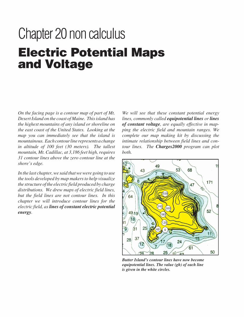
On the facing page is a contour map of part of Mt.Desert Island on the coast of Maine. This island hasthe highest mountains of any island or shoreline onthe east coast of the United States. Looking at themap you can immediately see that the island ismountainous. Each contour line represents a changein altitude of 100 feet (30 meters). The tallestmountain, Mt. Cadillac, at 3,186 feet high, requires31 contour lines above the zero contour line at theshore’s edge.

In the last chapter, we said that we were going to usethe tools developed by map makers to help visualizethe structure of the electric field produced by chargedistributions. We drew maps of electric field lines,but the field lines are not contour lines. In thischapter we will introduce contour lines for theelectric field, as lines of constant electric potentialenergy.

We will see that these constant potential energylines, commonly called equipotential lines or linesof constant voltage, are equally effective in map-ping the electric field and mountain ranges. Wecomplete our map making kit by discussing theintimate relationship between field lines and con-tour lines. The Charges2000 program can plotboth.

CHAPTER 20 ELECTRIC POTENTIAL MAPS AND VOLTAGE

Butter Island’s contour lines have now becomeequipotential lines. The value (gh) of each lineis given in the white circles.

20-2 Electric Potential Maps and Voltage

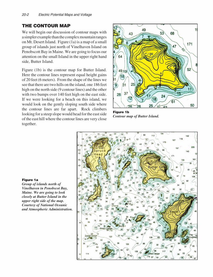
THE CONTOUR MAPWe will begin our discussion of contour maps witha simpler example than the complex mountain rangeson Mt. Desert Island. Figure (1a) is a map of a smallgroup of islands just north of Vinelhaven Island onPenobscott Bay in Maine. We are going to focus ourattention on the small Island in the upper right handside, Butter Island.

Figure (1b) is the contour map for Butter Island.Here the contour lines represent equal height gainsof 20 feet (6 meters). From the shape of the lines wesee that there are two hills on the island, one 186 feethigh on the north side (9 contour lines) and the otherwith two bumps over 140 feet high on the east side.If we were looking for a beach on this island, wewould look on the gently sloping south side wherethe contour lines are far apart. Rock climberslooking for a steep slope would head for the east sideof the east hill where the contour lines are very closetogether.

Figure 1bContour map of Butter Island.

Figure 1aGroup of islands north ofVinelhaven in Penobscot Bay,Maine. We are going to lookclosely at Butter Island in theupper right side of the map.Courtesy of National Oceanicand Atmospheric Administration.

Electric Potential Maps and Voltage 20-3

Although we would rather picture this island as beingin the south seas, our island is in the North Atlantic,and we will imagine that a storm has just covered itwith a sheet of ice. You are standing at the pointlabeled A in Figure (1), and start to slip. If the surfaceis smooth, which way would you start to slip?

A contour line runs through Point A which we haveshown in an enlargement in Figure (2). You wouldnot start to slide along the contour line because allthe points along the contour line are at the sameheight. Instead, you would start to slide in thesteepest downhill direction, which is perpendicularto the contour line as shown by the arrow.

Figure 2The direction youwould start to slip,the direction ofsteepest descent, isperpendicular tothe contour lines.

If you do not believe that the direction of steepestdescent is perpendicular to the contour line, chooseany smooth surface like the top of a rock, mark ahorizontal line (an equal height line) for a contourline, and carefully look for the directions that aremost steeply sloped down. You will see that allalong the contour line the steepest slope is, in fact,perpendicular to the contour line.

Skiers are familiar with this concept. When youwant to stop and rest and the slope is icy, you plantyour skis along a contour line so that they will notslide either forward or backward. The direction ofsteepest descent is now perpendicular to your skis, ina direction that ski instructors call the fall line. Thefall line is the direction you will start to slide if theedges of your skis fail to hold.

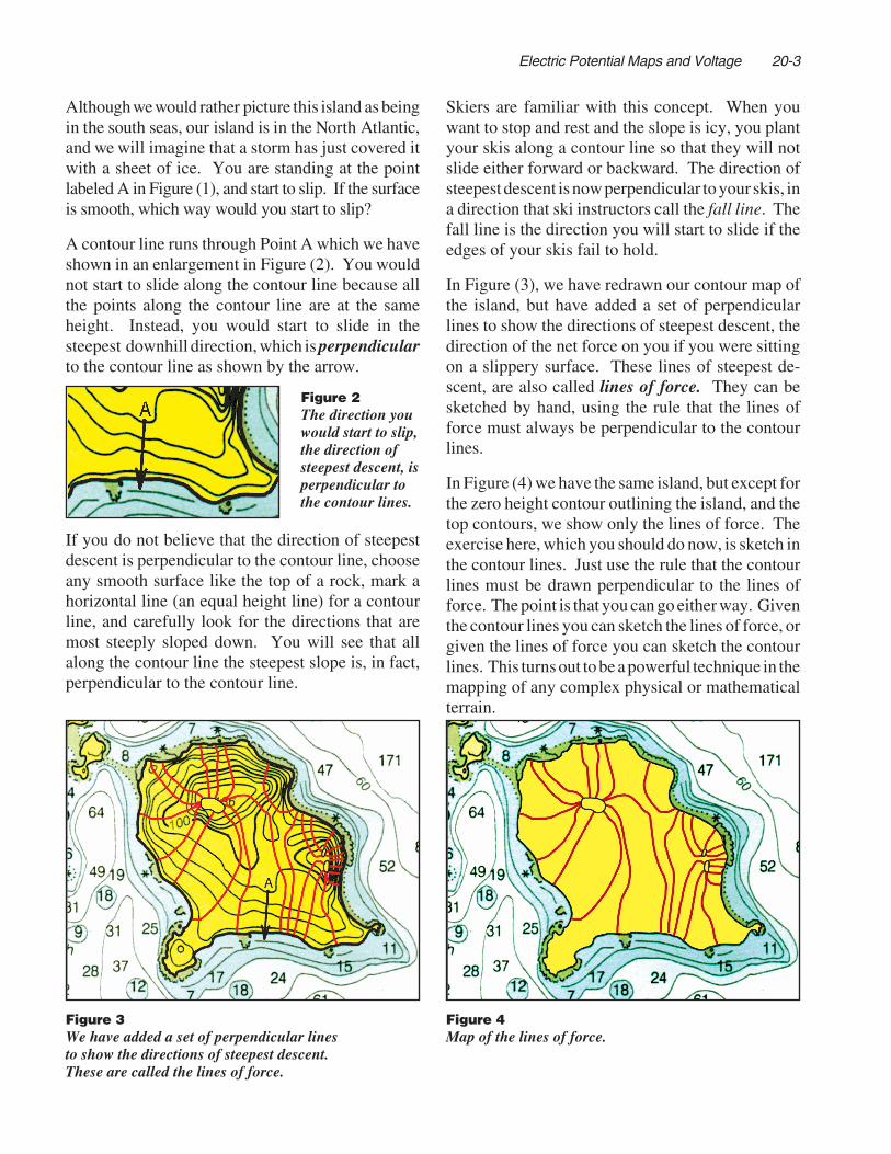
In Figure (3), we have redrawn our contour map ofthe island, but have added a set of perpendicularlines to show the directions of steepest descent, thedirection of the net force on you if you were sittingon a slippery surface. These lines of steepest de-scent, are also called lines of force. They can besketched by hand, using the rule that the lines offorce must always be perpendicular to the contourlines.

In Figure (4) we have the same island, but except forthe zero height contour outlining the island, and thetop contours, we show only the lines of force. Theexercise here, which you should do now, is sketch inthe contour lines. Just use the rule that the contourlines must be drawn perpendicular to the lines offorce. The point is that you can go either way. Giventhe contour lines you can sketch the lines of force, orgiven the lines of force you can sketch the contourlines. This turns out to be a powerful technique in themapping of any complex physical or mathematicalterrain.

Figure 4Map of the lines of force.

Figure 3We have added a set of perpendicular linesto show the directions of steepest descent.These are called the lines of force.


GRAVITATIONAL POTENTIALThe lines in a contour map give us the lines ofconstant height in the terrain. If you walk along acontour line you neither gain or lose height h orgravitational potential energy mgh (where m is yourmass). As a result, another name for these contour linescould be “lines of constant gravitational potential en-ergy”.

If we are to draw maps of potential energy ratherthan height, we do not want the m in the formulamgh because m is your mass, and a different personwould want to use a different mass. We can solvethis problem by drawing maps of constant potentialenergy of a unit mass (m = 1 kg), and call the result(gh) the gravitational potential. In Figure (5) wehave redrawn the contour map of Butter Island, butlabeled the contour lines with their values of gravi-tational potential (gh) in MKS units rather than h infeet. The difference in gravitational potential be-tween lines, instead of being 20 feet, is now

gh = 9.8metersec2 × 20 ft × .3048meter

ft

gh = 60meters2

sec2

difference ingravitationalpotential betweencontour lines

(1)

You can see that with gh having the dimensions of meters2/sec2 , that mgh has the dimensions kg meters2/sec2

which is the same as kinetic energy 1/2mv2 . That set of dimensions is called a joule.

If a 50 kg person climbed from one contour line tothe next (from one equipotential line to the next) theamount of gravitational potential energy she wouldgain would be

energygained

= mgh

= 50 kg×60m2

sec2

= 300 joules

(2)

Since we get the gravitational potential energy injoules by multiplying the gravitational potential (gh)by the mass m of the person climbing, we can see thatthat the gravitational potential has the dimensions ofjoules/kilogram.

gravitationalpotential

= ghjoules

kg (3)

Figure 5Butter Island’s contour lines have now becomeequipotential lines. The value (gh) of each line is givenin the white circles.


ELECTRIC POTENTIALDrawing contour maps for the electric field involvessteps similar to what we just did for the contour mapof gravitational potential.

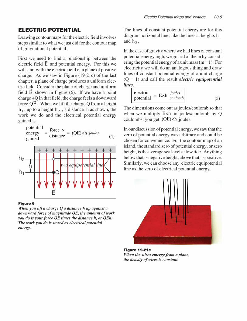
First we need to find a relationship between theelectric field E and potential energy. For this wewill start with the electric field of a plane of positivecharge. As we saw in Figure (19-21c) of the lastchapter, a plane of charge produces a uniform elec-tric field. Consider the plane of charge and uniformfield E shown in Figure (6). If we have a pointcharge +Q in that field, the charge feels a downwardforce QE . When we lift the charge Q from a height

h1 , up to a height h2 , a distance h as shown, thework we do and the electrical potential energygained is

potentialenergygained

=force ×distance

= (QE)×h joules(4)

The lines of constant potential energy are for thisdiagram horizontal lines like the lines at heights h1and h2 .

In the case of gravity where we had lines of constantpotential energy mgh, we got rid of the m by consid-ering the potential energy of a unit mass (m = 1). Forelectricity we will do an analogous thing and drawlines of constant potential energy of a unit charge(Q = 1) and call the result electric equipotentiallines.

electricpotential = E×h

joulescoulomb (5)

The dimensions come out as joules/coulomb so thatwhen we multiply E×h in joules/coulomb by Qcoulombs, you get (QE)×h joules.

In our discussion of potential energy, we saw that thezero of potential energy was arbitrary and could bechosen for convenience. For the contour map of anisland, the standard zero of potential energy, or zeroheight, is the average sea level at low tide. Anythingbelow that is negative height, above that, is positive.Similarly, we can choose any electric equipotentialline as the zero of electrical potential energy.

Figure 6When you lift a charge Q a distance h up against adownward force of magnitude QE, the amount of workyou do is your force QE times the distance h, or QEh.The work you do is stored as electrical potentialenergy.

Figure 19-21cWhen the wires emerge from a plane,the density of wires is constant.

+ + + + + + + + + + +

Q

h2

hh

1

E

two equipotential lines


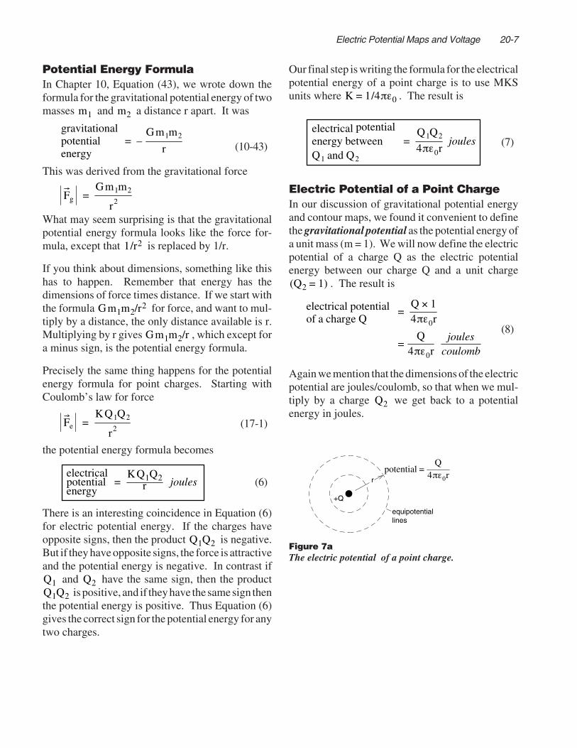
ELECTRIC POTENTIALOF A POINT CHARGEAt the end of the last chapter we discussed theelectric fields of a point charge, a line charge and aplane of charge. If we want to draw contour maps forthese three fields, the answers are quite obvious. Fora point charge the equipotential surfaces are concen-tric spheres centered on the charge as indicated inFigure (7). For a line charge, the equipotentialsurfaces are concentric cylinders centered on theline.

For a plane of charge where the field lines arestraight out from the plane, the equipotential sur-faces are planes parallel to the plane of charge, asindicated back in Figure (6).

To calculate the potential difference between twosurfaces for the point and line charges requires thecalculation of the amount of work we do in movinga charge from one surface to another. This calcula-tion is relatively easy using calculus, but difficultwithout. We faced this problem back in Chapter 10when we tried to calculate the change ingravitational potential energy when an object wascarried far from the surface of the earth. We willbriefly review the results of our gravitational discus-sion and apply the results to determine potentialenergies for point charges.

Gravitational Potential Energyof a Point MassWhen we discussed the potential energy of objectsacting as point masses, like the earth and sun, or theearth and a satellite, it was not convenient to choosethe surface of the earth as the zero of potentialenergy. Instead we said that two masses m1 and m2have zero potential energy when they are so far apartthat we can almost neglect the gravitational forcebetween them.

If the two masses were the only masses in theuniverse, and we left them at rest very far apart, therewould still be a tiny attractive gravitational force. Ifwe came back later, we would see the masses start-ing to move toward each other. As we watched, theirspeed would gradually increase, until finally theywould crash into each other at relatively high speeds.Just before they hit, they would have quite a bit ofkinetic energy. Where did this kinetic energy comefrom?

Obviously the kinetic energy came from gravita-tional potential energy, just as when we drop a ballon the floor. But we said that the two masses, whenvery far apart, had no gravitational potential energy.Starting from zero potential energy how could theyconvert potential energy into kinetic energy? Justthe same way you can write checks on a bankaccount that started with a zero balance. Both yourbalance and the ball’s potential energy becomenegative.

In talking about electric potential energy of pointcharges, we use the same convention. We say that ifthe charges are very far apart, their electrical poten-tial energy is zero. If we have a positive and anegative charge that attract each other like our twomasses, the electrical potential energy becomes nega-tive as the charges approach each other.

If, however, we have two charges of the same signthat repel each other, we have to push them togetherto get them near each other. The work we do pushingthem together is stored as positive electrical poten-tial energy. Once we have them together, and let go,the charges will fly apart, converting the potentialenergy we supplied into kinetic energy.

Thus if we use the convention that potential energyis zero when particles are far apart, then attractiveforces have negative potential energy, while repul-sive forces have positive potential energy.

+Q

r

equipotentiallines

electricfield lines

Figure 7The electric potential is the potential energy of apositive unit test charge qtest = + 1 coulomb.


Potential Energy FormulaIn Chapter 10, Equation (43), we wrote down theformula for the gravitational potential energy of twomasses m1 and m2 a distance r apart. It was

gravitationalpotentialenergy

= –Gm1m2

r (10-43)

This was derived from the gravitational force

Fg =

Gm1m2

r2

What may seem surprising is that the gravitationalpotential energy formula looks like the force for-mula, except that 1/r2 is replaced by 1/r.

If you think about dimensions, something like thishas to happen. Remember that energy has thedimensions of force times distance. If we start withthe formula Gm1m2/r2 for force, and want to mul-tiply by a distance, the only distance available is r.Multiplying by r gives Gm1m2/r , which except fora minus sign, is the potential energy formula.

Precisely the same thing happens for the potentialenergy formula for point charges. Starting withCoulomb’s law for force

Fe =

KQ1Q2

r2 (17-1)

the potential energy formula becomes

electricalpotentialenergy

=KQ1Q2

r joules (6)

There is an interesting coincidence in Equation (6)for electric potential energy. If the charges haveopposite signs, then the product Q1Q2 is negative.But if they have opposite signs, the force is attractiveand the potential energy is negative. In contrast if

Q1 and Q2 have the same sign, then the product Q1Q2 is positive, and if they have the same sign then

the potential energy is positive. Thus Equation (6)gives the correct sign for the potential energy for anytwo charges.

Our final step is writing the formula for the electricalpotential energy of a point charge is to use MKSunits where K = 1/4πε0 . The result is

electrical potentialenergy betweenQ1 and Q2

=Q1Q2

4πε0rjoules (7)

Electric Potential of a Point ChargeIn our discussion of gravitational potential energyand contour maps, we found it convenient to definethe gravitational potential as the potential energy ofa unit mass (m = 1). We will now define the electricpotential of a charge Q as the electric potentialenergy between our charge Q and a unit charge

(Q2 = 1) . The result is

electrical potentialof a charge Q

=Q × 14πε0r

=Q

4πε0rjoules

coulomb

(8)

Again we mention that the dimensions of the electricpotential are joules/coulomb, so that when we mul-tiply by a charge Q2 we get back to a potentialenergy in joules.

+Q

r

equipotentiallines

potential =

Q4πε0r

Figure 7aThe electric potential of a point charge.


ELECTRIC VOLTAGEIn our discussion of Bernoulli’s equation, we gavethe collection of terms (P + ρgh + 1/2ρv2) the namehydrodynamic voltage. The content of Bernoulli’sequation is that this hydrodynamic voltage is con-stant along a stream line when the fluid is incom-pressible and viscous forces can be neglected. Twoof the three terms, ρgh and 1/2ρv2 represent theenergy of a unit volume of the fluid, thus we see thatour hydrodynamic voltage has the dimensions ofenergy per unit volume.

Electric voltage is a quantity with the dimensions ofenergy per unit charge that in different situations isrepresented by a series of terms like the terms inBernoulli’s hydrodynamic voltage. There is thepotential energy of an electric field, the chemicalenergy supplied by a battery, even a kinetic energyterm, seen in careful studies of superconductors, thatis strictly analogous to the 1 21 2ρv2 term in Bernoulli’sequation. In other words, electric voltage is acomplex concept, but it has one simplifying feature.Electric voltages are measured by a common experi-mental device called a voltmeter. In fact we will takeas the definition of electric voltage, that quantitywhich we measure using a voltmeter.

This sounds like a nebulous definition. Withouttelling you how a voltmeter works, how are you toknow what the meter is measuring? To overcomethis objection, we will build up our understanding ofwhat a voltmeter measures by considering the vari-ous possible sources of voltage one at a time.Bernoulli’s equation gave us all the hydrodynamicvoltage terms at once. For electric voltage we willhave to dig them out as we find them.

Our first example of an electric voltage term is theelectric potential energy of a unit test charge. Thishas the dimensions of energy per unit charge whichin the MKS system is joules/coulomb and calledvolts.

1

joulecoulomb

≡ 1 volt (9)

Figure (8) shows the electric field lines and equipo-tential lines for a point charge Q. We see fromEquation (8) that a unit test particle at Point (1) hasa potential energy, or voltage V1 given by

V1 =

Q

4πε0r1

electricpotentialorvoltage at Point(1)

At Point (2), the electric potential or voltage V2 isgiven by

V2 =

Q

4πε0r2

electricpotentialorvoltage at Point(2)

Voltmeters have the property that they only measurethe difference in voltage between two points. Thusif we put one lead of a voltmeter at Point (1), and theother at Point (2), as shown, then we get a voltagereading V given by

voltmeterreading

V ≡ V2 – V1 =Q

4πε0

1r2

–1r1

(10)

If we put the two voltmeter leads at points equaldistances from Q, i.e., if r1 = r2 , then the voltmeterwould read zero. Since the voltage difference be-tween any two points on an equipotential line is zero,the voltmeter reading must also be zero when theleads are attached to any two points on an equipoten-tial line.

This observation suggests an experimental way tomap equipotential lines or surfaces. Attach one leadof the voltmeter to some particular point, call it Point(A). Then move the other lead around. Wheneveryou get a zero reading on the voltmeter, the second

r2

r1

+

–voltmeter

V

1

2

Figure 8A voltmeter measures the difference in electricalvoltage between two points.


lead must be at another point of the same equipoten-tial line as Point (A). By marking all the pointswhere the meter reads zero, you get a picture of theequipotential line.

The discussion we have just given for finding theequipotential lines surrounding a point charge Q isnot practical. This involves electrostatic measure-ments that are extremely difficult to carry out. Justthe damp air from your breath would affect thevoltages surrounding a point charge, and typicalvoltmeters found in the lab cannot make electrostaticmeasurements. Sophisticated meters in carefully con-trolled environments are required for this work.

But the idea of potential plotting can be illustratednicely by the simple laboratory apparatus illustratedin Figure (9). In that apparatus we have a tray ofwater (slightly salty or dirty, so that it is somewhatconductive), and two metal cylinders attached bywire leads to a battery as shown. There are also twoprobes consisting of a bent, stiff wire attached to ablock of wood and adjusted so that the tips of thewires stick down in the water. The other end of theprobes are attached to a voltmeter so we can read thevoltage difference between the two points (A) and(B), where the probes touch the water.

If we keep Probe (A) fixed and move Probe (B)around, whenever the voltmeter reads zero, Probe(B) will be on the equipotential line that goes through

brasscylinders

tap water pyrex dish

battery

VA

B

probes

voltmeter

Point (A). Without too much effort, one can get acomplete plot of the equipotential line. Each timewe move Probe (A) we can plot a new equipotentialline. A plot of a series of equipotential lines is shownin Figure (10).

Once we have the equipotential lines shown inFigure (10), we can sketch the lines of force bydrawing a set of lines perpendicular to the equipo-tential as we did in Figure (11). With a little practiceyou can sketch fairly accurate plots, and the beautyof the process is that you did not have to do anycalculations!

Figure 9Simple setup for plotting fields. You plotequipotentials by placing one probe (A) at a givenposition and moving the other (B) around.Whenever the voltage V on the voltmeter readszero, the probes are at points of equipotential.

A

Figure 11To draw field lines, draw smooth lines, alwaysperpendicular to the equipotential lines, andmaintain any symmetry that should be there.

Figure 10Plot of the equipotential lines from a student project byB. J Grattan. Instead of a tray of water, Grattan used asheet of conductive paper, painting two circles withaluminum paint to replace the brass cylinders.


A Field Plot ModelThe analogy between a field plot and a map maker’scontour plot can be made even more obvious byconstructing a plywood model like that shown inFigure (12).

To construct the model, we made a computer plot ofthe electric field of charge distribution consisting ofa charge +3 and –1, seen on the next page in Figure(13). We enlarged the computer plot and then cut outpieces of plywood that had the shapes of the contourlines. The pieces of plywood were stacked on top ofeach other and glued together to produce the threedimensional view of the field structure.

In this model, each additional thickness of plywoodrepresents one more equal step in the electric poten-tial or voltage. The voltage of the positive charge Q= +3 is represented by the fat positive spike that goesup toward + ∞ and the negative charge q = –1 isrepresented by the smaller hole that heads down to– ∞ . These spikes can be seen in the back view inFigure (12), and the potential plot in Figure (14).

In addition to seeing the contour lines in the slabs ofplywood, we have also marked the lines of steepestdescent with narrow strips of black tape. These linesof steepest descent are always perpendicular to thecontour lines, and are in fact, the electric field lines,when viewed from the top as in the photograph ofFigure (13).

Figure (15) is a plywood model of the electricpotential for two positive charges, Q = +5, Q = +2.Here we get two hills, somewhat like Butter Island.

–1

+3–.1V

–.2V

–.3V

–.4V

.1V

.2V

.3V

.4V

.5V

.6V

.7V

.8V

.9V

1.0V

1.1V

1. 2V

Figure 12Model of the electric field in the region of two pointcharges Q+ = + 3, Q– = – 1. Using the analogy to atopographical map, we cut out plywood slabs in theshape of the equipotentials from the computer plot ofFigure (13), and stacked the slabs to form a threedimensional surface. The field lines, which aremarked with narrow black tape on the model, alwayslead in the direction of steepest descent on the surface.

Figure 15Model of the electric potential in the regionof two point charges Q = +5 and Q = +2.

Figure 14Potential plot alongthe line of the twocharges +3, –1. Thepositive chargecreates an upwardspike, while thenegative chargemakes a hole.


V = .1

V = .2

V = .3

V = .4

V = .5

V = .1

V=

–.

1

V=

.0

–1 +3 Figure 13Computer plot of the field lines and equipotentials for a chargedistribution consisting of a positive charge + 3 and a negative charge – 1.These lines were then used to construct the plywood model. (We areassuming that the thickness of the plywood represents a step of .1 volts.)


COMPUTER PLOTSIn order to construct the plywood models we justsaw, we used computer plots of the equipotentiallines surrounding the charges. These lines becomethe contour lines of the voltage landscape producedby the charges.

At the end of the previous chapter we described thefairly complex way we drew the fields lines of a chargedistribution. The calculation of the equipotential linesis much easier to describe. What we do is use thevoltage formulas like Equation (10) to calculate thevoltage at each pixel in the plotting board. Then wechange the pixel color at specified voltage intervals.

For example, suppose the voltage ranges from –4volts up to 12 volts and we want equipotential linesat 1 volt intervals. We plot all the pixels in the range–4 volts to –3 volts in the minus voltage color, whichis blue for the standard colors. Then we leave aswhite all the pixels in the –3 volt to –2 volt range. Thosein the –2 volt to –1 volt range are blue again. We usethe same scheme for the positive voltages, except weuse pink for the standard positive voltage color.

To show how to obtain voltage plots, we start inFigure (16) with the field line plot of two pointcharges placed to match our experimental plot ofFigure (11) reproduced here. We then go to the toolspalette and use the pull down menu to select “Chooseboth 2D” which means to plot both the field lines andvoltage colors for a two dimensional plot. Pressing“Plot” we got the result shown in Figure (18).

Figure 16Field lines for two point charges.

Figure 17Selecting to plotboth field andequipotentiallines.

Figure 18Field and equipotential lines for two point charges.

Figure 11Equipotentiallines from astudent project.We sketched inthe field lines.

A

You should notice that the lines separating colors inFigure (18) are fairly close to the experimentalequipotential lines of the student project in Figure(11).

Our reasoning for choosing pink, white and blue forthe standard colors came from using red for positivecharges and voltages and blue for negative ones. Welet the field lines remain black. The color scheme isclear but hardly inspiring. Back in Figure (19a) inthe last chapter, we showed how to chose a differentcolor scheme for more interesting plots. Figure (18)looks a lot better if you plot using “UnderwaterColors”. We leave it up to the reader to find out whatthe result is.


The Color PaletteIf you want some reallyinteresting results, youcan use the Color Paletteshown in Figure (19).That control panel allowsyou to change the color ofany area or line in theplot. For example, if youwant to change the pinkcolor of positive voltages,you click on the pink areain the palette. A crossappears where youclicked and the three colorsliders show the value ofthe color in the clickedarea. Instead of havingyou choose the amount ofred, green, and blue, thestandard for TV screencolors, we give you the choice of Hue, Saturationand Brightness. Play with these sliders and you willquickly see what these terms mean, and why they aremuch more convenient than trying to express a colorin terms of how much red, green and blue are in themixture. Figures (20) and (21) are examples of whatyou can accomplish using the Color Palette.

Figure 19Color Palette.

Suggested Laboratory WorkBecause the computer program is available, wesuggest that you do something more creative in thelab than simply plotting the equipotential lines oftwo charges. We leave the choice up to the studentand instructor, but would very much like to see anyinteresting results.

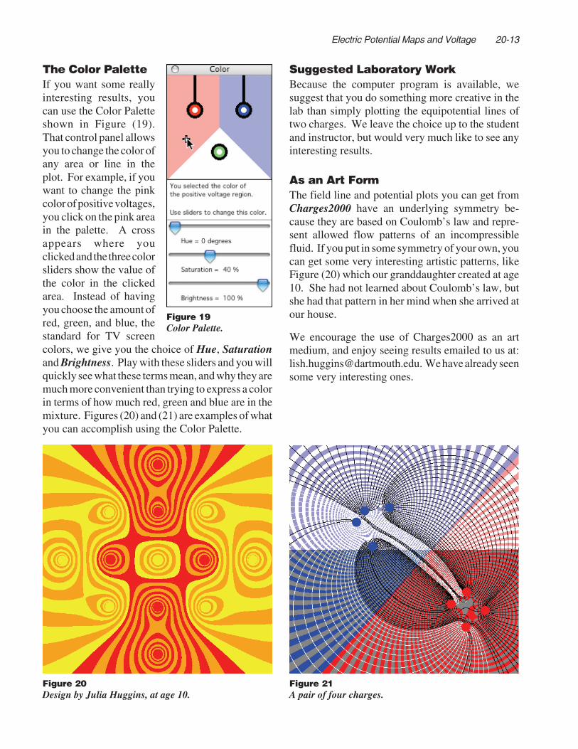
As an Art FormThe field line and potential plots you can get fromCharges2000 have an underlying symmetry be-cause they are based on Coulomb’s law and repre-sent allowed flow patterns of an incompressiblefluid. If you put in some symmetry of your own, youcan get some very interesting artistic patterns, likeFigure (20) which our granddaughter created at age10. She had not learned about Coulomb’s law, butshe had that pattern in her mind when she arrived atour house.

We encourage the use of Charges2000 as an artmedium, and enjoy seeing results emailed to us at:[email protected]. We have already seensome very interesting ones.

Figure 20Design by Julia Huggins, at age 10.

Figure 21A pair of four charges.


CHAPTER 20 REVIEWThe aim of this chapter is to apply mapmaker’stechniques to describe and visualize the electricfield E .

We began with a contour map of a small island, amap showing contour lines of equal height h. InFigure (5) we relabeled the contour lines as lines ofgravitational potential gh. The name gravitationalpotential came from the fact that gh is the gravita-tional potential energy mgh of a unit massm = 1 kilogram.

Earlier, in Figure (3) we drew another set of linesthat are everywhere perpendicular to the contourlines. These are the lines along which you wouldstart to slide if the island were covered with a sheetof ice in an ice storm. They are called lines of forceand are directed in the most downhill direction,which is always perpendicular to the horizontalcontour lines.

In the last chapter we introduced the electric fieldlines E which show the direction of the force on aunit test charge qtest = 1 coulomb. These are alsocalled lines of force. In this chapter, instead of goingfrom contour lines to lines of force as we did for thegravitational potential, we went the other way. Westarted with the lines of force and drew a set ofperpendicular lines which represented lines of con-

stant electric potential. These lines of constant elec-tric potential are the lines along which our unit testcharge qtest has constant electric potential energy.

Another name for the electric potential energy of aunit charge is voltage. The set of lines perpendicu-lar to the electric field lines are lines of constantvoltage.

For working with electric phenomena, we have aconvenient way to measure voltage, at least differ-ences in voltage between two points. That device iscalled a voltmeter.

To become familiar with how a voltmeter can beused to study electric fields, we have a very impor-tant laboratory exercise. By placing a couple ofbrass cylinders in a tray of tap water, and attachinga battery of voltage Vb across the cylinders, we setup a voltage difference in the water between thecylinders. We then attached two probes to thevoltmeter. We set one probe at some location in thewater and move the other probe around in the wateruntil the voltmeter reads zero volts. That means thatthe two probes are located on the same constantvoltage line. You have thus located two points on avoltage contour line. Moving the second probearound you can locate a number of points on thiscontour line and then sketch the line.

Figure 3We have added a set of perpendicular linesto show the directions of steepest descent.These are called the lines of force.

Figure 5Butter Island’s contour lines have now becomeequipotential lines. The value (gh) of each line is givenin the white circles.


Once we have drawn the voltage contour lines, wecan, as in Figure (3), then draw the perpendicularset of electric field lines. We did this in going fromFigure (10) to Figure (11), starting with a student’sexperimental constant voltage lines.

In Figure (12) we showed how to construct a threedimensional model of the electric voltage contourlines and electric field lines for a charge Q – = – 1coulomb near a charge Q + = + 3 coulombs. Withthis model you can see that there is a completeanalogy between electric field and voltage maps,and the mapmaker’s contour maps.

In the previous chapter we introduced the computerprogram Charges2000 for drawing the electricfield lines produced by various distributions ofcharge. Another feature of the program is that ateach point on the plotting board, it calculates the

electric voltage produced by the charge distribu-tion. By using the same color to plot all points in acertain voltage range, say, from 1 volt to 2 volts, thena different color for all points in the next range, say,from 2 volts to 3 volts, the voltage contour lines liealong the borders where the color changes.

Comparing Figures (11) and (18) on page 20-12, wesee that the computer plot and the student’s lab workare close.

CHAPTER EXERCISESThe important lessons from this chapter are:

(1) Develop an intuitive feeling for the perpendicu-lar sets of lines, one marking lines of constantvoltage, the other, lines for force.

(2) Become familiar with using a voltmeter to mea-sure lines of constant voltage.

(3) Become familiar with the use of Charges2000to plot both field lines and voltage contours.

Working numerical problems is not the aim of thischapter.brass

cylinders

tap water pyrex dish

battery

VA

B

probes

voltmeter

A

Figure 9Experimental setup.

Figure 11Equipotential and field lines from student project.

Figure 18Field and equipotential lines for two point charges.

chapter 20 non calculus - physics2000

Documents