1

Chapter 2.1 in Handbook of Process Integration

Heat Integration − Targets and Heat Exchanger Network Design

Truls Gundersen Department of Energy and Process Engineering

Norwegian University of Science and Technology

Kolbjoern Hejes vei 1.A, NO-7491 Trondheim, Norway

 

Abstract ...................................................................................................................................... 2  

1   Introduction to Key Concepts and Major Topics ................................................................ 2  

2   Stages in Design of Heat Recovery Systems ...................................................................... 6  

3   Data Extraction ................................................................................................................... 8  

3.1   Data required for basic Heat Integration .................................................................... 8  

3.2   Major Challenges in Data Extraction ......................................................................... 9  

4   Performance Targets ......................................................................................................... 12  

4.1   Minimum External Heating and Cooling ................................................................. 14  

4.2   Minimum Number of Heat Exchangers ................................................................... 18  

5   Process Modifications ....................................................................................................... 21  

5.1   Plus/Minus Principle and Appropriate Placement ................................................... 22  

5.2   Grand Composite Curve and Correct Integration .................................................... 25  

6   Network Design ................................................................................................................ 28  

6.1   The Pinch Design Method ....................................................................................... 29  

6.2   Developing an initial MER Design .......................................................................... 30  

6.3   A Strategy for Stream Splitting ............................................................................... 33  

7   Design Evolution .............................................................................................................. 35  

7.1   A Three-way Trade-off in Network Design ............................................................ 36  

7.2   Using Loops and Paths to evolve Network Design ................................................. 37  

8   Concluding Remarks ......................................................................................................... 42  

9   Sources of further Information .......................................................................................... 43  

References ................................................................................................................................ 43  

2

Abstract

This chapter describes the basic steps of Pinch Analysis for heat recovery that made Process

Integration a methodology employed by numerous designers and engineers worldwide and

made industrial leaders in the 1980s claim these concepts to be the results of academic

research with the largest impact on industrial thinking related to design and operation in the

process industries. Key elements of the chapter are the Heat Recovery Pinch, Performance

Targets ahead of design, and a step-wise and systematic procedure for Heat Exchanger

Network Design. One of the main characteristics of Pinch Analysis is the extensive use of

Graphical Diagrams and Representations that give the designer a good overview of even the

most complex processes. These tools provide insight and ease the communication between

designers and engineers.

Keywords: Heat Recovery Pinch; Composite Curves; Performance Targets; Pinch Design

Method; Design Evolution

1 Introduction to Key Concepts and Major Topics

This section provides a brief introduction to the history, the major topics and the key concepts

of Heat Integration, while subsequent sections will provide more details about performance

targets, graphical diagrams and representations, as well as design procedures that form the

basis of the methodology, with a few simple and illustrating examples to assist the

explanations in the text. The section repeats and expands parts of Chapter 1.2 on Basic

Terminology of Process Integration. Heat Integration was an early (“pioneering”) activity and

is still an important part of the “discipline” that today is referred to as Process Integration.

The term Heat Integration has two meanings. First, it refers to the physical arrangement of

equipment, process sections, production plants, entire sites, and even the surroundings in case

of district heating or district cooling. Second, it refers to an area of Process Synthesis, with

methods and tools aiming at increased energy efficiency in industrial processes and energy

plants. Such improved energy efficiency can be achieved by combining (i.e. integrating)

heating and cooling demands and thereby reducing the need for external heating and cooling

3

utilities. Efficient use of equipment is of course also part of the scope, since energy efficiency

only becomes interesting and will be implemented if it is economically feasible.

The birth of Process Integration as a Systems oriented design activity is related to the

discovery of the concept referred to as the Heat Recovery Pinch. A methodology coined

Pinch Analysis was developed in the late 1970s and early 1980s, which resulted in a departure

from traditional design practice that had been based on extending and improving process

technologies by the use of operating and engineering insight (i.e. following the “learning

curve”) and to choose the best design from a set of case studies. Of course, there would

occasionally be discoveries and breakthroughs that made step changes possible, but the

uncertainty whether designs could be further improved and by how much, was still left with

the designer. Most of the text in this chapter on Heat Integration will focus on increasing

Energy Efficiency of processing systems, using Pinch Analysis as the main methodology.

The most important new feature in Pinch Analysis was the ability to establish Performance

Targets ahead of design only based on information about the change in thermodynamic state

for the process streams, described in table form and hereafter referred to as Stream Data.

These targets were first developed for thermal energy (external heating and cooling) and have

later been extended to mechanical energy (power or shaft work), number of heat exchangers,

and total heat transfer area. In fact, by using analogies, the original Heat Pinch concept and

the idea of targeting ahead of design have been re-used (as indicated in Chapter 1.2 and

several other chapters of this Handbook) in other areas such as mass exchange processes

(Mass Pinch), wastewater minimisation and distributed effluent treatment systems (Water

Pinch), hydrogen management in oil refineries (Hydrogen Pinch), and oxygen consuming

processes (Oxygen Pinch). Similar ideas have also been applied to study for example Supply

Chains and Carbon Emission reductions.

The concept of a Heat Recovery Pinch was independently discovered and developed by

Hohmann (1971), Huang and Elshout (1976), Linnhoff et al. (1978,1979) and Umeda et al.

(1978). The basic idea is to draw separately the total heating and the total cooling

requirements of a process in a cumulative manner in a Temperature – Enthalpy diagram,

commonly referred to as Composite Curves. Similar drawings had already been used by

designers of low temperature processes such as air separation (Linde AG in Germany) to

4

design multi-stream heat exchangers (Gundersen, 2000). The graphical construction of

Composite Curves is explained with an example in Section 4.1.

Heat recovery between hot and cold streams is restricted by the shape of the Composite

Curves and the fact that heat can only be transferred from higher to lower temperature. The

minimum allowed temperature difference ( ) is an economic parameter that indicates a

near optimal trade-off between investment cost (heat exchangers) and operating cost (energy).

The point of smallest vertical distance (equal to ) between the Composite Curves

represents a bottleneck for heat recovery and is referred to as the Heat Recovery Pinch.

An alternative representation of the overall heating and cooling demands in a process is the

Heat Cascade, a special case of the transshipment model from Operations Research. Here, hot

streams (i.e. “sources” of heat) contribute to a set of temperature intervals (i.e. “warehouses”

of heat), while cold streams (i.e. “sinks” of heat) draw heat from the same intervals. The

temperature intervals are established on the basis of the supply and target temperatures of all

process streams. A heat balance is made for each temperature interval, and any heat surplus in

one interval is cascaded (thus the name) down to the next interval with lower temperatures.

The Heat Cascade also forms the basis of the Grand Composite Curve (also referred to as the

Heat Surplus Diagram), a very important tool for studying the interface between the process

and the utility system (consumption and generation of various types of utilities, both load and

level) and for evaluating heat integration of special equipment such as Distillation Columns,

Evaporators, Heat Pumps and Heat Engines. The graphical construction of Heat Cascades and

the Grand Composite Curve is explained with an example in Section 5.2.

Perhaps the most important property of the Heat Recovery Pinch is that it decomposes the

process into a heat deficit region above Pinch and a heat surplus region below Pinch. There is

not enough heat available in the hot streams above Pinch to satisfy the overall heating demand

of the cold streams, and external heating is required. Below Pinch, there is not enough cooling

available in the cold streams to satisfy the overall cooling demand of the hot streams, and

external cooling is required. Based on the insight about this Pinch Decomposition,

systematic, general and step-wise design procedures have been developed for heat exchanger

networks with minimum energy consumption.

ΔTmin

ΔTmin

5

Pinch Decomposition also forms the basis of more general rules for design modifications as

well as integration of special equipment, heat and power considerations and beyond. The

Plus/Minus Principle states that any design modification aiming to reduce external heating

and cooling should result in (1) an increase (“Plus”) in the duty of hot streams above Pinch or

cold streams below Pinch, and/or (2) a decrease (“Minus”) in the duty of colds streams above

Pinch or hot streams below Pinch, where (1) and (2) often can be combined. The Appropriate

Placement concept is based on the same philosophy and can be stated in general terms as the

placement (or integration) of heat sources above Pinch and heat sinks below Pinch.

As indicated above, Pinch Decomposition is the basis for the Pinch Design Method (PDM)

adopted and extensively used in a large number of industrial sectors such as, but not limited

to, oil & gas, chemical & petrochemical, pulp & paper, metal production, dairies, breweries

and pharmaceuticals. Any heat leakage from the higher temperature region above Pinch (with

heat deficit) to the lower temperature region below Pinch (with heat surplus) results in an

increase of both hot and cold utilities; thus there is a Double Penalty associated with such

heat transfer. The main philosophy behind the PDM (Linnhoff and Hindmarsh, 1983) is thus

to avoid any cross Pinch heat transfer by designing separate heat exchanger networks above

and below Pinch. PDM is a step-wise (sequential) design procedure that provides rules for

selection of hot and cold streams to be matched in heat exchangers, the sequence and duty of

the heat exchangers, the need for stream splitting, etc.

This chapter describes tools and methods for designing new plants, often referred to as

Grassroots Design, while a much more common activity in industry is the improvement of

existing plants by making investments that increase production volumes and/or process

efficiency. The latter is often referred to as Retrofit Design where, as explained in Chapter

2.5, the main objective is to reduce energy consumption in existing process plants by

increasing the level of heat recovery. The design project then focuses on investing in some

new equipment, repiping or changing internals in heat exchangers, while making maximum

use of existing units. Heat exchangers are tailor-made, thus there is no second hand market

and equipment that is purchased and installed should be kept as part of the modified design.

6

2 Stages in Design of Heat Recovery Systems

As indicated above, there is a fundamental difference between designing heat exchanger

networks for new designs (“grassroots”) and modifying heat recovery systems for existing

plants (“retrofit”). At the same time, the design process contains the same stages for the two

cases, however, with quite different content, as will be explained in Section 3.2 and Chapter

2.5. More specifically, the stages in design of heat recovery systems are:

• Data Extraction

• Performance Targets

• Process Modifications

• Network Design

• Design Evolution

• Process Simulation

Data Extraction means collecting and processing data about heating and cooling

requirements as well as the need for evaporation and condensation of process streams, often

referred to as Stream Data. Similar data must be collected for systems available for external

heating and cooling, often referred to as Utility Data. Finally, Economic Data are needed,

such as cost of heat exchangers and utilities, economic parameters, etc. For grassroots,

consistent data are normally available from rigorous mass and energy balances established by

process simulators, however, the quality of the data depends on whether or not the simulation

model is a good representation of the actual process. For retrofit, data could also be taken

from process simulations; alternatively data collected from measurements could be used. In

the latter case, some data reconciliation is required after removing obvious (or “gross”) errors.

Performance Targets refer to establishing measures for best performance ahead of design

only based on information available in the Stream Data, Utility Data and Economic Data (the

type of data that is needed depends on the actual target(s) to be obtained). Typical targets for

heat exchanger networks include minimum external heating and cooling

demands, fewest number of heat exchangers , and minimum total heat transfer area

. With multiple utilities, targets can also be established for the cost optimal utility mix.

(QH,min ) (QC,min )

(Umin )

(Amin )

7

Process Modifications refer to the consideration of making changes in the basic process

(reactor system, separation system, recycle system, etc.) in such a way that the scope for heat

recovery is improved. The indicator for the potential advantage of making such process

changes is the Composite Curves established during the Performance Targets stage, and the

tool for suggesting these changes is the Plus/Minus principle mentioned in Section 1.

Network Design in this chapter means establishing a network of heat exchangers that achieves

the Performance Targets for energy consumption and number of heat exchangers, referred to

as an MER design (Maximum Energy Recovery). The primary tool for network design is the

Pinch Design Method (PDM) mentioned in Section 1, which is fundamentally based on the

Pinch Decomposition principle. Separate networks are established above and below Pinch

based on firm rules for matching hot and cold process streams in heat exchangers, rules for

the sequence of these units, and a strategy for stream splitting when favorable or required.

Design Evolution primarily means to refine MER designs by removing small heat exchangers

resulting from the use of the PDM, where separate networks are developed above and below

Pinch. This activity is also referred to as Energy Relaxation, since removing units will require

more utilities (energy) and possibly also more heat transfer area. The motivation for this stage

is cost reduction as well as reduction in network complexity (fewer units, which is often

followed by fewer stream splits). The tools are the degrees of freedom in the network referred

to as Stream Splits, Heat Load Loops and Heat Load Paths that will be described in Section

7.1.

Finally, Process Simulation in this context means testing the feasibility of the heat exchanger

network that has been designed and optimised in the previous stages of the design process.

This stage may also involve switching from simplified models of pure counter-current heat

exchangers to more practical and realistic design configurations. However, to describe the

Process Simulation stage is regarded to be beyond the scope of this chapter.

8

3 Data Extraction

Data Extraction is a very time consuming and critical activity, since the quality and realism of

the design solutions depend heavily on the correctness of the data. The saying “garbage in

means garbage out” also applies here.

3.1 Data required for basic Heat Integration

The type of data required for Heat Integration projects obviously relate to the need for

heating, cooling, evaporation and condensation in the process. In short, what is needed is a

quantification of the required enthalpy changes of the process streams. From thermodynamics,

the change in the total enthalpy flow, H (kW), that a process stream undergoes when changing

conditions can be obtained from [3.1].

[3.1]

where m is mass flowrate (kg/s) and h is specific enthalpy (kJ/kg), giving change in enthalpy

flow the units of (kJ/s = kW). Enthalpy is in general a complicated function of stream

pressure, temperature and composition. In Heat Integration, a process stream is defined as one

that does not change mass flowrate or composition. Whenever such changes take place, a new

process stream is introduced. If we assume constant mass flowrate and stream composition,

and ignore the effect of pressure on enthalpy, then [3.1] can be simplified to [3.2].

[3.2]

where is the specific heat capacity at constant pressure (kJ/kgK). In order to replace

numerical integration by simple summation, the assumption of a constant or a piece-wise

linear relation between temperature and enthalpy has been extensively used in Pinch Analysis.

If is assumed constant, and the supply and target temperatures of a process stream are

denoted and respectively, then [3.2] is simplified even further to [3.3].

[3.3]

ΔH = m ⋅dh∫

ΔH = m ⋅ cp ⋅dT∫

cp

cp

cp

TS TT

ΔH = m ⋅cp ⋅ dTTS

TT

∫ = CP ⋅(TT −TS )

9

where CP is a lumped parameter (the product of m and ) that is referred to as the “heat

capacity flowrate” with units (kW/K). For process streams changing phase, information about

the latent heat of such phase changes would be required. It should be emphasized that in this

chapter, no formal sign convention is made, rather common sense is applied. This means that

both hot and cold streams have changes in enthalpy flow that are positive as indicated in [3.4],

where subscripts h and c refer to hot and cold process streams respectively. By definition, a

hot process stream is one that is being cooled and/or condensed, while a cold process stream

is one being heated and/or evaporated.

[3.4]

If the relationship between temperature and enthalpy is non-linear, either caused by a non-

constant or a phase change, improved accuracy in the analysis can be obtained by dividing

process streams into piece-wise linear substreams often referred to as stream segments. This

improves the targeting part (Section 4), while it adds complexity to the network design

(Section 6), since one needs to keep track of the relationship between stream segments and the

original process streams when suggesting heat exchangers in the network.

The data described above are sufficient to establish targets for minimum external heating and

cooling in the process, as soon as a value for the minimum allowed temperature difference

mentioned in Section 1, , is established. When information about the utility system (the

number of different utility types for external heating and cooling) is available, targets for the

minimum number of heat exchangers (often referred to as units) can be established. In order

to calculate targets for minimum total heat transfer area in the heat recovery systems, data for

film heat transfer coefficients, h (kW/m2K), for process streams and utilities are also required.

3.2 Major Challenges in Data Extraction

There are two very different types of challenges related to data extraction for a Heat

Integration project:

(i) To establish the most correct set of data related to flowrates and thermodynamic

conditions of process streams used as input to heat recovery analysis and design.

cp

ΔHh = CPh ⋅(TS ,h −TT ,h ) and ΔHc = CPc ⋅(TT ,c −TS ,c )

cp

ΔTmin

10

(ii) To represent the heating, cooling, evaporation and condensation needs of the process

streams in such a way that the degrees of freedom are kept open for network design.

While activity (i) is fairly straightforward (but involves a lot of work), activity (ii) requires

skills and experience. It has often been stated that data extraction (in particular the second

part) is more art than science, thus most of the attempts to provide procedures and guidelines

for this activity has failed, including the development of knowledge based systems (also

referred to as expert systems). Some of the commercial general purpose process simulators

have features for automatic stream data extraction on the basis of a converged steady state

mass and energy balance calculation. While these procedures enable easy generation of

Composite and Grand Composite Curves, they do not keep the degrees of freedom open.

Despite the importance of data extraction, the topic has not been much discussed in the

literature beyond text-books on Process Integration, such as Linnhoff et al. (1982), Smith

(2005) and Kemp (2007). The topic is also thoroughly covered in the recent book by Klemeš

et al. (2010). Interestingly, rather detailed literature on data extraction has been provided in

the form of reports from research institutes (such as CANMET, 2003), software vendors (such

as AspenTech, 2009) and consulting companies (such as Linnhoff March, 1998), which again

illustrates the importance of proper data extraction for a successful heat integration project.

For manual data extraction, the following guidelines can be useful:

a) Do not copy all features of the conceptual flowsheet or an existing design.

b) Do not mix streams at different temperatures.

c) Do not include utilities as stream data.

d) Do not accept the prejudice of colleagues against heat integration.

e) Do not ignore true practical constraints.

f) Distinguish between soft and hard stream data.

Rule (a) refers to the issue of keeping the degrees of freedom open in order not to overlook

promising solutions for heat recovery systems. Rule (b) involves several aspects and should

be discussed in more depth. First, a mixer can act as a heat exchanger, thus saving capital

cost, however, mixing streams with different composition is only an option if the streams are

entering the same unit operation, such as a chemical reactor. Second, mixing streams at

11

different temperatures introduces exergy losses and should be avoided. Third, mixing streams

may eliminate potential heat recovery solutions. Finally, mixing streams may be required

from a practical point of view, such as adding steam to hydrocarbon streams to avoid coking

inside pipes and equipment, or it may be forbidden from a safety point of view, such as

mixing oxygen rich streams with hydrocarbon streams. Rule (c) is rather obvious, since the

goal of the exercise is to establish minimum utility requirements, however, there are cases

where it is not so easy to distinguish whether a stream is a process stream or acts as a utility.

Rule (d) relates to the common reluctance in the process industries to accept heat integration

solutions from an operational point of view, however, it is a fact that most industrial processes

are heavily integrated, and rather than focusing on maximum heat recovery, one should focus

on correct or appropriate heat integration. In addition, it should be mentioned that when the

economical potential of heat integration is established and well documented, it is often easier

to get acceptance for such projects. Rule (e) means that even though one should try to keep

the degrees of freedom open, obviously one should not forget that some practical constraints

cannot be ignored. One example is related to metal dusting, a severe form of corrosive

degradation of metals that happens in some temperature range when CO is present. This is a

problem in synthesis gas production, and in order to keep the metal temperature at a

sufficiently low level, the boiler is placed upstream of the steam superheater, which is not the

best solution from a thermodynamic point of view as conveyed in Pinch Analysis.

Finally, rule (f) is quite important in the sense that some stream data must be considered as

hard specifications, while others can be adjusted if that improves or simplifies the heat

recovery system (as discussed in Chapter 1.2 on Basic Terminology of Process Integration).

An inlet temperature to a reactor or distillation column must often be regarded as a hard

specification, while the target temperature of a process stream going to some sort of storage is

an example of soft process data. Specifying a low target temperature for a hot product stream

going to storage in order to increase the heat recovery potential will only result in increased

need for external cooling if the target temperature is below the Pinch temperature. Instead,

this cooling could have been taken care of by nature itself through convective heat losses to

the environment.

12

Returning to activity (i) of the data extraction exercise there are two distinctly different

situations. For grassroots design, there is normally a simulation model available for the

process providing stream data as part of a steady state material and energy balance

calculation. The advantage in this case is that the data are consistent. As an example, the hot

and cold side of a heat exchanger will always be in balance for a converged simulation. The

quality of the data, however, depends on to what extent the simulation models describes the

behavior of the real process.

For retrofit design, in addition to using a simulation model if available, one could resort to the

original specification sheets for the process, or one could use measurements from the plant.

However, the plant may have been modified several times since its start-up, and flowsheets

and specification sheets are not always updated. Regarding the use of measurements, the

typical situation is that some measurements are missing, and instruments may either not be

functioning at all, or they may give incorrect readings. In such cases, the task of data

reconciliation can be enormeous, and a key to success is to work very close with operators

and plant engineers.

4 Performance Targets

In order to illustrate the different stages in the design of heat recovery systems, consider the

very simple process example in Fig. 4.1, where two feed streams (A and B) are heated before

entering a chemical reactor where a product and a by-product are produced. The main product

is then recovered in the bottoms stream from a distillation column, while the by-product and

traces of unreacted raw material (feed) is taken from the top of the same distillation column.

Fig. 4.1 also indicates the supply and target temperatures of the process streams as well as the

lumped parameter CP (“heat capacity flowrate”) in brackets with units (kW/K). Notice that

heat exchangers are not included, since these will be the result of the Heat Integration study.

It is important at this stage to emphasize that “heat capacity flowrate” (CP = mCp) is different

from mass flow rate (m). This is why the reactor effluent (CP = 100) is less than the sum of

the reactor inlets (CP = 50 + 150 = 200). The explanation in this case is that feed stream B is

subject to evaporation before entering the reactor. Since the outlet temperature from the

reactor is higher than the inlet temperature, the chemical reactions taking place must be

13

exothermic. Based on the flowsheet in Fig. 4.1 and the given data for temperatures, heat

capacity flowrates and duties for the distillation column reboiler and condenser, the stream

data resulting from data extraction (Section 3) are listed in Table 4.1.

Figure 4.1 Simple Process used as an Illustrative Example

Table 4.1 Stream Data for the Simple Process in Fig. 4.1

ID Description TS (°C) TT (°C) CP (kW/K) ΔH (kW)

H1 Reactor Effluent 220 130 100 9,000

H2 Main Product 130 50 90 7,200

C1 Feed A 40 150 50 5,500

C2 Feed B 80 150 150 10,500

CON Column Condenser 120 120 n.a. 3,000

REB Column Reboiler 130 130 n.a. 3,000

ST Steam for heating 250 250 n.a. variable

CW Cooling Water 20 30 n.a. variable

For distillation columns, the heating and cooling requirements are normally given as the

duties of the reboiler and the condenser. The reflux and boil-up are circulating internal

streams in the column and therefore normally not measured. This means that the CP values

150°C

80°C

40°C

50°C

130°C

120°C

130°C 220°C 150°C

Reactor

Distillation Column

By-product

Product Feed A

Feed B

50⎡⎣⎢

⎤⎦⎥

150⎡⎣⎢

⎤⎦⎥

100⎡⎣⎢

⎤⎦⎥

90⎡⎣⎢

⎤⎦⎥

10⎡⎣⎢

⎤⎦⎥

CW

ST

3 MW

3 MW

14

are not available (n.a.) as indicated in Table 4.1. The duties of steam and cooling water are

listed as “variable” in Table 4.1, which is obvious since these are the unknowns that will be

found as a result of the energy targeting exercise.

4.1 Minimum External Heating and Cooling

As mentioned in Section 1, targets for heat recovery systems depend on the specification of a

minimum allowed temperature difference for heat transfer, , which is an economic

parameter for the trade-off between investment cost (heat exchangers) and operating cost

(energy). Given a value for this parameter, targets for minimum external heating, , and

minimum external cooling, , can be obtained by graphical or numerical methods

established in the early period of Pinch Analysis. The graphical representations are referred to

as Composite and Grand Composite Curves, while there are several numerical methods such

as the Problem Table Algorithm (Linnhoff and Flower, 1978) and the Heat Cascade

(Linnhoff, 1979). Actually, Hohmann (1971) was the first to provide a systematic way to

obtain energy targets by his Feasibility Table. The Heat Cascade will be used in this chapter

since it (i) provides a nice illustration of the heat flows and decompositions in heat recovery

systems and (ii) provides the necessary information to construct the Grand Composite Curve.

Optimisation techniques such as Linear and Mixed Integer Programming (LP and MILP) can

also be used to obtain targets for minimum external heating and cooling as well as targets for

the fewest number of heat exchangers, especially in more complicated situations such as for

example when there are forbidden matches between hot and cold process streams. These

optimisation techniques will be briefly discussed in Chapter 2.5.

Composite Curves

Composite Curves have been described and applied by a number of authors, such as Huang

and Elshout (1976), Umeda et al. (1978) and Linnhoff et al. (1982). The Composite Curves

(T-H diagram) are constructed by dividing the temperature axis into intervals based on the

supply ( ) and target ( ) temperatures of the process streams, and to add together the

enthalpy contributions (hot streams) and requirements (cold streams) in each temperature

interval. Finally, these enthalpies are drawn in a cumulative manner against the corresponding

temperatures, resulting in one curve for the hot streams and one curve for the cold streams.

ΔTmin

QH ,min

QC ,min

TS TT

15

These curves are then positioned relative to each other in such a way that the Hot Composite

Curve (the cooling curve) is always above the Cold Composite Curve (the heating curve). In

this way, heat can be recovered in the overlapping region of the Composite Curves. This

“positioning” in the T-H diagram is obtained by shifting the two curves horizontally. Moving

the curves closer together means increased heat recovery, and the economic limit is when the

smallest vertical distance between the curves becomes equal to , while the

thermodynamic limit is when this vertical distance becomes zero. The point where the vertical

distance between the Composite Curves is at its minimum (and equal to ) acts as a

bottleneck against increased heat integration and has therefore been referred to as the Heat

Recovery Pinch.

Composite Curves for the stream data in Table 4.1 are shown in Figure 4.2 for .

Key information about the heat recovery system can be obtained from this graphical diagram,

such as the process Pinch, maximum heat recovery, and the corresponding minimum external

heating and cooling requirements. Reading accurate information from such diagrams can be

somewhat difficult, which is why numerical methods are often preferred. The real advantage

of such graphical diagrams, however, is that they provide an overview of the system and they

contribute strongly to the understanding of the problem. One such insight is that any heat

leakage from the region above Pinch to the region below Pinch (cross Pinch heat transfer) will

result in increased need for both hot and cold utilities (i.e. double penalty).

Figure 4.2 Composite Curves for the Illustrative Example

ΔTmin

ΔTmin

ΔTmin = 20°C

0 5 10 15 20 25 H (MW)

T (°C)

0

50

100

150

200

250

Process Pinch

ΔTmin

QH ,min

QC,min

16

Based on the Composite Curves in Fig. 4.2, approximate targets for minimum external

heating and cooling seem to be in the range 3.0-3.5 MW. As indicated above, there are also a

number of numerical methods that can be applied to obtain these targets more accurately. Fig.

4.3 shows the Heat Cascade for the same illustrative example with stream data in Table 4.1.

The reboiler (REB) and the condenser (CON) of the distillation column adds two rather

strange temperature intervals to the heat cascade, since it is assumed that condensation and

evaporation in these units take place at constant temperature. This means that the streams with

sensible heat (H1, H2, C1, and C2) do not deliver or extract any heat from these intervals that

are marked with a “+” and a “-“ for the corresponding temperatures.

Heat Cascade

The heat cascade is an example of the Transhipment Model from Operations Research, with

sources, warehouses and sinks. The hot streams are drawn as sources of heat on the left hand

side of the cascade, with corresponding hot stream temperatures. The cold streams are drawn

as sinks of heat on the right hand side of the cascade, with corresponding cold stream

temperatures. All supply and target temperatures of the process streams should be represented

as interval temperatures in the cascade; in addition there will be “corresponding” temperatures

on the “opposite” side obtained by adding to the supply and target temperatures of cold

process streams and subtracting from the supply and target temperatures of hot process

streams. This means that the specification of a minimum temperature difference is built into

the heat cascade. Any heat exchange taking place in the temperature intervals of Fig. 4.3 will

be feasible and satisfy the requirement that .

As indicated in Fig. 4.3, the hot streams provide heat to the temperature intervals according to

their cooling requirements, and the cold streams extract heat from the temperature intervals

according to their heating requirements. Heat balances are established for each interval, and

any surplus of heat in one interval is cascaded (thus the name “heat cascade”) as a heat

residual ( ) to the next interval with lower temperatures. Since none of these residuals can

be negative (would indicate transfer of heat from lower to higher temperatures which is

infeasible with heat exchangers), the minimum external heating requirement can be identified

as the minimum heat needed to make these residuals non-negative.

ΔTmin

ΔTmin

ΔT ≥ ΔTmin

Rk

17

A simple, yet powerful way to establish values for and is to start by assuming

in Fig. 4.3. The heat residuals can then be obtained for the entire heat cascade in

a sequential manner as follows:

R1 =QH + 5,000 = +5,000 kW R2 = R1 − 2,000 = +3,000 kW R3 = R2 − 3,000 = 0 kWR4 = R3 − 2,000 = −2,000 kW R5 = R4 −1,100 = −3,100 kW R6 = R5 + 3,000 = −100 kWR7 = R6 − 2,200 = −2,300 kW R8 = R7 +1,600 = −700 kW QC = R8 + 900 = 200 kW

Figure 4.3 Heat Cascade for the Illustrative Example

As mentioned above, negative residuals are infeasible when designing a system of heat

exchangers, and residual has the largest negative value of the entire heat cascade. This

QH ,min QC ,min

QH = 0 kW

+ 5,000

- 2,000

- 3,000

- 2,000

- 1,100

+ 3,000

- 2,200

+ 1,600

+ 900

ST

CW

H1

H2

CON

REB

C1

C2

220°C 200°C

170°C 150°C

150+°C 130+°C

150−°C 130−°C

120+°C 100+°C

120−°C 100−°C

130°C 110°C

100°C 80°C

60°C 40°C

50°C 30°C

QH

R1

R2

R3

R4

R5

R6

R7

R8

QC

5,000

2,000

2,000

900

1,800

3,600

900

3,000

1,000

3,000 3,000

1,000

3,000 500

1,500

3,000

1,000

2,000

R5

18

residual then becomes the bottleneck (i.e. Heat Recovery Pinch), and minimum external

cooling is found to be QH ,min = 3,100 kW . The corresponding minimum external heating is

then QC ,min = 3,300 kW , and the process Pinch is defined by the temperatures 120°C (for hot

streams) and 100°C (for cold streams). Since the residual actually is related to the

temperatures 120+°C and 100+°C, it means that the column condenser (CON) is supplying

heat below Pinch. The implications of this will be discussed in Sections 5.1 and 5.2.

4.2 Minimum Number of Heat Exchangers

The next logical step in a Heat Integration project is to establish targets for the fewest number

of heat exchangers, also referred to as units. This is done by the so-called ( ) rule, used

for the first time by Hohmann (1971). Linnhoff et al. (1979) explained that the ( ) rule is

a simplification of Euler’s Rule from graph theory ( ). The analogy between

graphs and heat exchanger networks is that nodes represent streams, while edges represent

heat exchangers. Thus N is the total number of process streams and utility types, U is the

number of heat exchangers (units), L is the number of independent loops, and S is the number

of sub-networks (or subgraphs). Since the objective is to establish a target for the number of

units ahead of design, network related features such as loops and sub-networks are not known.

This is overcome by setting (loops can be removed as will be shown in Section 7.2)

and (conservative, since the presence of sub-networks reduces the number of units). As

a result, Euler’s Rule reduces to . As pointed out in Section 1, however, separate

networks must be designed above and below Pinch in order to achieve the targets for

minimum external heating and cooling. Thus, the ( ) rule has to be applied separately

above and below Pinch in order to have a target for the number of units that is compatible

with the heating and cooling targets. A targeting formula for minimum number of units in a

heat exchanger network achieving Maximum Energy Recovery (MER) is then given by [4.1].

[4.1]

As will become evident in Section 7.2, the fewest number of units in heat recovery systems

that relax the MER requirement (do not decompose at the Pinch) is another useful target value

and is given by [4.2].

R5

1N −

1N −

U N L S= + −

0L =

1S =

1U N= −

1N −

Umin,MER = (Nabove −1)+ (Nbelow −1)

19

[4.2]

Grid Diagram

Another invention from the pioneering period of Pinch Analysis is the Grid Diagram, which is

an alternative way to draw heat exchanger networks. While the grid diagram is a departure

from standard ways to represent process flowsheets, it has the important advantage that it

mimics the desirable counter-current flow of heat exchangers and thereby makes it easy to

implement Pinch decomposition in heat exchanger networks as well as to study cross Pinch

heat transfer. Fig. 4.4 shows the grid diagram for the illustrative example presented in Figs.

4.1-4.3. Contrary to the first version of this representation proposed by Linnhoff (1979) the

Handbook follows the more logical form, where temperatures increase from left to right, as

they would do in any xy diagram. This then defines the directions of the hot and cold process

streams in the diagram. It should also be emphasized that no linear temperature scale is

applied; rather the main focus is on whether a stream is present above, across or below Pinch.

Figure 4.4 Grid Diagram for the Illustrative Example

While the grid diagram will act as a “drawing board” for network design in subsequent

sections, the first use of this representation is to establish targets for minimum number of heat

Umin,global = (Ntotal −1) = (NH + NC + NUtil −1)

C1

C2

REB

H1

H2

CON

220°C

130°C

150°C

150°C

130°C 130°C

120°C 120°C

50°C

130°C 120°C

40°C

80°C

100°C

20

exchangers. In this respect, heat exchangers (or units) refer to process-to-process heat

exchangers as well as utility exchangers (such as steam heaters and water coolers). The

dashed lines in Fig. 4.4 indicate the “position” of the process Pinch, and all streams are drawn

relative to these Pinch temperatures. Thus, similar to the heat cascade, the grid diagram also

keeps track of both hot and cold stream temperatures. Utilities could also have been included

in the grid diagram (particularly useful with multiple utilities), but has been left out for the

sake of simplicity. It should be emphasized that targeting for units takes place after targeting

for energy, thus the types and amounts of different utilities needed are known and fixed.

The grid diagram can be used to set targets for the fewest number of units as follows: For an

MER design, Pinch decomposition must be obeyed, and [4.1] can be applied. Energy targeting

established the need for both steam (3,100 kW) and cooling water (3,300 kW). Above the

Pinch, there are 2 hot streams (H1 and H2), 3 cold streams (C1, C2 and REB), and 1 hot

utility (ST). Below the Pinch, there are 2 hot streams (H2 and CON), 2 cold streams (C1 and

C2), and 1 cold utility (CW). The MER target for minimum number of units then becomes:

Similarly, the target for the fewest number of units when strict Pinch decomposition is

relaxed, can be found by [4.2]:

This mans that the penalty for Maximum Energy Recovery (and strict Pinch decomposition) is

that two (i.e. 9−7) more heat exchangers are likely to be required in the network. This issue

will be further discussed in Section 7.2

Targeting methods have also been developed for minimum total heat transfer area, fewest

number of heat exchanger shells (rather than units) for situations where shell & tube

exchangers are dominating, and total annual cost. The latter can be used to identify a

reasonable value for (also referred to as pre-optimisation or SuperTargeting). These

more advanced targets will be presented in Chapter 2.5. Further targets that will be discussed

in other chapters of the Handbook involve mechanical energy, such as shaftwork targets, and

targets for total sites (both heat and power).

Umin,MER = (Nabove −1)+ (Nbelow −1) = (2 + 3+1−1)+ (2 + 2 +1−1) = 5 + 4 = 9

Umin,global = (Ntotal −1) = (3+ 3+ 2 −1) = 7

ΔTmin

21

5 Process Modifications

With Composite Curves established and Performance Targets calculated, it makes sense to

consider options for Process Modifications before continuing with Network Design. The

shape of the Composite Curves indicates whether potentials for increased heat recovery exist,

and what actions are needed to reduce external heating and cooling for the process. Ideally,

the Composite Curves should be as parallel as possible, since this allows for a high level of

heat recovery. In reality, the Composite Curves will have kinks or “knees” that act as

bottlenecks (Pinch points), which will limit heat recovery. One way to make the Composite

Curves more parallel is to move some of these kinks to other temperatures or to remove some

of the kinks completely, with main focus on the near Pinch region of the process.

In addition, the fundamental feature of having a heat deficit region above the process Pinch

and a heat surplus region below the process Pinch provides guidelines for how the process

should be modified to increase the potential for heat recovery. These guidelines, later coined

the Plus/Minus Principle, have been discussed again in various ways by Umeda et al. (1979),

Linnhoff and Parker (1984) and Linnhoff and Vredeveld (1984). The Plus/Minus Principle

suggests that above Pinch, one should try to increase the amount of heat provided by hot

streams (+) or decrease the amount of heat required by cold streams (−). Likewise, below

Pinch, one should try to increase the amount of heat required by cold streams (+) or decrease

the amount of heat provided by hot streams (−). This means that if a hot stream (or part of it)

is moved from below to above Pinch or a cold stream (or part of it) is moved from above to

below Pinch, the situation improves in both regions. Such “moves” can be realized by

changing the temperature of streams, which in some cases results from changing the stream

pressure. Another possibility is to increase or reduce the enthalpy change of a stream.

Some obvious examples of process modifications include:

• Decrease the pressure and thus the boiling point temperature of an evaporator (cold

stream) to move the operation from above to below Pinch

• Split an evaporator into several stages in series (i.e. multi-effect)

• Decrease the pressure of a distillation column to move the reboiler (a cold stream)

from above to below Pinch

22

• Increase the pressure of a distillation column to move the condenser (a hot stream)

from below to above Pinch

• Change the reflux of a distillation column

• Change the feed preheating or precooling of a distillation column

• Change the operating conditions of a reactor

5.1 Plus/Minus Principle and Appropriate Placement

The Plus/Minus Principle also provides guidelines for integration (or Appropriate Placement)

of special equipment such as distillation columns (Linnhoff et al., 1983), evaporators (Smith

and Linnhoff, 1988) heat pumps and heat engines (Linnhoff and Townsend, 1982). The

background is that such equipment should not be integrated unless there are considerable

energy savings involved that will compensate for additional operating problems as well as any

increase in investment cost. The term Correct Integration has also been used, and the issue can

be addressed simply by considering the different units as sources and sinks of heat. For

obvious reasons, energy savings will only be made if one integrates a source of heat with a

sink of heat, and simple thermodynamic principles require that the source must have a higher

temperature than the sink. The following classification can be made for some of the typical

equipment mentioned above as well as for the “background” (or remaining) process:

• The background process as represented by its heat cascade is a heat sink above the

process Pinch and a heat source below the same Pinch

• A distillation column represents a heat sink in the reboiler and a heat source in the

condenser

• An evaporator represents a heat sink in the evaporation stage (boiler) and a heat source

in the condenser

• A heat pump represents a heat sink at lower temperature (evaporator) and a heat

source at higher temperature (condenser), while consuming mechanical energy

• A heat engine represents a heat sink at higher temperature and a heat source at lower

temperature, while producing mechanical energy

Correct use of a heat pump to reduce external heating in the background process then means

to integrate the source of the process below Pinch with the sink of the heat pump (evaporator)

as well as to integrate the source of the heat pump (condenser) with the sink of the process

23

above Pinch. In short, this means that the heat pump should be integrated across Pinch in the

sense that it utilizes heat from the surplus region below Pinch and supplies it to the deficit

region above Pinch. Such integration (or use) of a heat pump reduces both hot and cold utility

consumption. If a heat pump is integrated entirely above Pinch, the only result from an energy

point of view is that mechanical energy usage is converted into thermal energy savings on a

1:1 basis, which is not a good idea, since mechanical energy has a higher value. If a heat

pumps is integrated below Pinch, however, a much worse scenario can be drawn: Use of

mechanical energy in the heat pump only results in an increased consumption of cold utility.

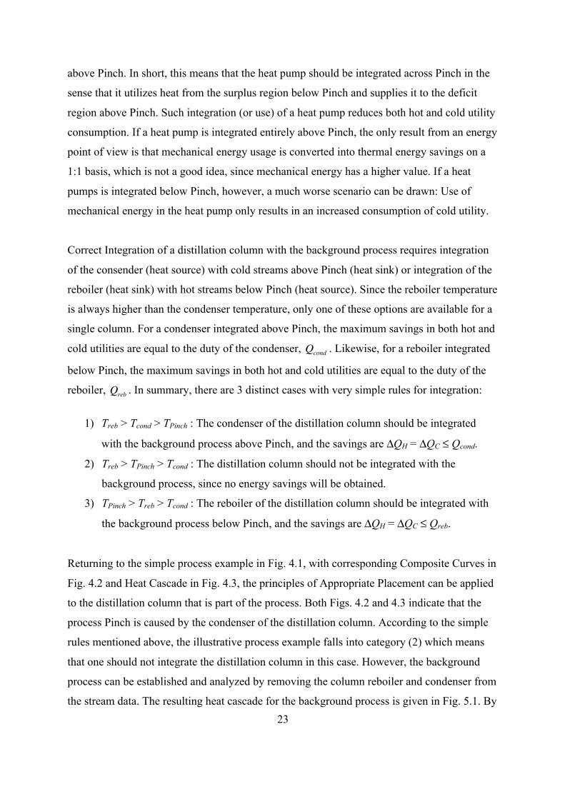
Correct Integration of a distillation column with the background process requires integration

of the consender (heat source) with cold streams above Pinch (heat sink) or integration of the

reboiler (heat sink) with hot streams below Pinch (heat source). Since the reboiler temperature

is always higher than the condenser temperature, only one of these options are available for a

single column. For a condenser integrated above Pinch, the maximum savings in both hot and

cold utilities are equal to the duty of the condenser, . Likewise, for a reboiler integrated

below Pinch, the maximum savings in both hot and cold utilities are equal to the duty of the

reboiler, . In summary, there are 3 distinct cases with very simple rules for integration:

1) Treb > Tcond > TPinch : The condenser of the distillation column should be integrated

with the background process above Pinch, and the savings are ΔQH = ΔQC ≤ Qcond.

2) Treb > TPinch > Tcond : The distillation column should not be integrated with the

background process, since no energy savings will be obtained.

3) TPinch > Treb > Tcond : The reboiler of the distillation column should be integrated with

the background process below Pinch, and the savings are ΔQH = ΔQC ≤ Qreb.

Returning to the simple process example in Fig. 4.1, with corresponding Composite Curves in

Fig. 4.2 and Heat Cascade in Fig. 4.3, the principles of Appropriate Placement can be applied

to the distillation column that is part of the process. Both Figs. 4.2 and 4.3 indicate that the

process Pinch is caused by the condenser of the distillation column. According to the simple

rules mentioned above, the illustrative process example falls into category (2) which means

that one should not integrate the distillation column in this case. However, the background

process can be established and analyzed by removing the column reboiler and condenser from

the stream data. The resulting heat cascade for the background process is given in Fig. 5.1. By

Qcond

Qreb

24

analyzing the temperature intervals in this case, it is obvious that the third interval will be the

limiting one, thus minimum external heating is given by the need to make R3 non-negative.

For the background process, the energy targeting exercise provides the following results:

• Process Pinch is given by R3 = 0, TPinch = 100°C/80°C (for hot/cold streams)

• Minimum external heating is given by QH,min = 3,300 + 4,000 − 5,000 = 2,300 kW

• Minimum external cooling is given by QC,min = 1,600 + 900 = 2,500 kW

Figure 5.1 Heat Cascade for the Background Process

These results are surprising and should be analyzed and explained. The simple rule applied

above indicated that no savings would be obtained by integrating the distillation column. The

background process needs 2,300 kW of external heating, while the reboiler of the column

needs 3,000 kW. In the non-integrated case, the total need for hot utility is then 2,300 + 3,000

= 5,300 kW. The assumption behind the Composite Curves (Fig. 4.2) and the total Heat

Cascade (Fig. 4.3) is that the distillation column is integrated with the background process.

The background for this statement is that the condenser and the reboiler are included in the

stream data in Table 4.1, which is the basis for Figs. 4.2 and 4.3. In the integrated case, the

calculated minimum external heating requirements are 3,100 kW, which means that despite

the predictions of the simple analysis above, heat integration of the column actually saves

5,300 − 3,100 = 2,200 kW. The reason for this apparent contradiction is that the Pinch for the

+ 5,000

- 4,000

- 3,300

+ 1,600

+ 900

ST

CW

H1

H2

C1

C2

220°C 200°C

170°C 150°C

130°C 110°C

100°C 80°C

60°C 40°C

50°C 30°C

QH

R1

R2

R3

R4

QC

5,000

4,000

2,700

3,600

900

6,000

2,000 4,500

1,500

2,000

25

background process (100°C/80°C) is different from the case when the distillation column is

integrated (120°C/100°C). In fact, distillation columns often cause Pinch points due to their

large duties at near constant temperature, a feature that results in marked “knees” on the

Composite Curves. With reference to the Pinch of the background process, the distillation

column operates entirely above Pinch and the example falls into category (1) above.

Another important result is that the savings are less than the duty of the integrated condenser

(2,200 < 3,000 = Qcond). Explaining this result requires use of another graphical diagram; the

Grand Composite Curve. While the simple rules can be used in a qualitative way to establish

whether Appropriate Placement is feasible or not, the Grand Composite Curve provides

quantitative information about the amount of heat that can be correctly integrated, and thus

how much heating and cooling that can be saved by Correct Integration.

5.2 Grand Composite Curve and Correct Integration

As mentioned when introducing the Heat Cascade in Section 1, one of its advantages is that it

provides the necessary information (or data) to construct the Grand Composite Curve

(Linnhoff et al., 1982). This is a diagram that shows the net accumulated heat surplus and heat

deficit in the process, and provides an excellent interface between the process and the utility

system. It can also be used to evaluate the integration of special equipment such as distillation

columns, heat pumps, etc. While the Composite Curves show two independent curves for hot

and cold process streams using real temperatures, the Grand Composite Curve (which is

another TH diagram) shows the residual of heat in the Heat Cascade as a single curve. Thus,

there is a need for a common temperature scale that can be used for both hot and cold process

streams, which is why the so-called “modified” temperatures have been introduced. The

simplest way to establish such modified temperatures is to subtract half of from hot

stream temperatures and likewise add half of to cold stream temperatures.

Considering the Heat Cascade in Fig. 5.1, this means that the average values of the hot and

cold interval temperatures will be used as the new temperature scale. A more advanced way to

establish modified temperatures is to introduce individual stream contributions to . This

allows for a more realistic approach to industrial problems where film heat transfer

coefficients may vary by one or two orders of magnitude. In such cases, the use of a single

ΔTmin

ΔTmin

ΔTmin

26

global value for is a gross over-simplification. Modified temperatures for hot streams

(i) and cold streams (j) are established by [5.1], where and are individual

contributions for hot and cold streams. The simple approach used in this chapter, however, is

that ΔTi = ΔTj = 0.5 ⋅ ΔTmin .

THi* = THi − ΔTi

TCj* = TCj + ΔTj

[5.1]

Figure 5.2 Grand Composite Curve for the Background Process

The Grand Composite Curve for the background process is shown in Fig. 5.2. This diagram

provides the same fundamental information as the Composite Curves (i.e. location of the

Pinch and minimum external heating and cooling), but it also hides information related to

process-to-process heat transfer. As a net Heat Surplus/Deficit Curve, the only process-to-

process heat transfer shown in the Grand Composite Curve, is the transfer of surplus heat

from one interval to another interval at lower temperature with heat deficit. This is referred to

as heat “pockets”, and the Grand Composite Curve in Fig. 5.2 has one such pocket.

The Grand Composite Curve not only shows the required external heating and cooling, it also

shows at what temperatures such external heating and cooling is required. This combination

of load and level is of course important information for utility placement, and can be used to

identify near-optimal consumption and possible production of various utility types. In

addition, as mentioned above, the Grand Composite Curve can be used to quantify how much

energy savings can be made by integrating distillation columns, evaporators, heat pumps and

ΔTmin

ΔTi ΔTj

0 2 4 5 6 8 H (MW)

T * (°C)

0

50

100

150

200

250

Process Pinch

QH ,min

7 3 1 QC,min

Heat Pocket

27

heat engines with the background process. Focusing on the illustrative example, Fig. 5.2

shows that the need for external heating is in the range from 90°C to 110.9°C (found by

interpolation) in modified temperatures, which means that the hot utility must have

temperatures between 120.9°C and 100°C to satisfy the specified of 20°C. Using steam

at 250°C as indicated in Table 4.1 would be a real waste of energy quality in this case, since

for example very low pressure steam at 121°C or hot water (or hot oil) operating between

121°C and 100°C would be sufficient.

As already stated, the Grand Composite Curve can be used to quantitatively address the issue

of Correct Integration. Since the simple process example in Fig. 4.1 includes a distillation

column, it will be used to illustrate how the Grand Composite Curve can be used to identify

the scope for integrating the column with the background process. A distillation column can

be plotted as a box in TH diagrams, where temperature profile and duty are plotted for the

condenser and the reboiler. In the illustrative example, condensation (120°C) and evaporation

(130°C) take place at constant temperature, and the duty of these units are equal (3 MW). The

box representation in a TH diagram then becomes a simple rectangle. When plotted together

with the Grand Composite Curve, modified temperatures must be used, which means that for

, the condenser (hot stream) should be plotted at 110°C, while the reboiler (cold

stream) should be plotted at 140°C. Fig 5.3 shows the Grand Composite Curve (GCC) for the

background process and the distillation column plotted in the same TH diagram.

Figure 5.3 Background Process GCC and Distillation Column

ΔTmin

ΔTmin = 20°C

0 2 4 5 6 8 H (MW)

T * (°C)

0

50

100

150

200

250 QH ,min

7 3 1 QC,min

28

The solid rectangle in Fig. 5.3 is in conflict with the GCC, and feasible heat transfer (meaning

) between the condenser and the background process is limited to 2,200 kW

(found by interpolation in the GCC for a modified temperature of 110°C). If, however, the

pressure of the column is increased slightly, the condenser and reboiler temperatures will

increase accordingly, and the enthalpy box representing the column would fit into the heat

pocket of the GCC. Increasing pressure will in most cases make the separation more difficult,

thus there is a need for more equilibrium stages in the column or more reflux (with a balanced

trade-off, this normally means an increase in both number of stages and reflux). This is

indicated in Fig. 5.3 by making the dashed rectangle for the column after pressure increase

somewhat wider along the enthalpy axis, since reboiler and condenser duties are proportional

to the reflux.

In summary for this example, the background process requires 2,300 kW of external heating

while the distillation column needs 3,000 kW heating in the reboiler, a total of 5,300 kW.

Total cooling is correspondingly 2,500 + 3,000 = 5,500 kW. By integrating the column

condenser with cold streams above the Pinch, it is possible to utilize 2,200 kW of the

condenser duty. This means that 2,200 kW of savings are made in external heating (41.5%) as

well as cooling (40%). However, using process modifications, in this case a slight increase in

the column pressure, makes it possible to integrate the entire condenser and save 3,000 kW of

external heating (56.6%) and cooling (54.6%). The disadvantage with this last scheme that

saves an additional 800 kW, is the need to integrate both the condenser (totally) and the

reboiler (partly) with corresponding operational challenges related to the control of the

column.

6 Network Design

With performance targets for energy and units, the next step is the actual design of the heat

exchanger network. One of the most significant features of Pinch Analysis is that the insight

obtained in establishing performance targets ahead of design actually forms the core of the

design methodology. The discovery of the Heat Recovery Pinch in the early and late 1970s

was followed by the understanding that in order to design heat exchanger networks with

minimum external heating and cooling requirements, decomposition at the Pinch and the

development of two independent networks were absolute requirements.

ΔT ≥ ΔTmin

29

6.1 The Pinch Design Method

The Pinch Design Method (PDM) was outlined by Linnhoff and Turner (1981) and also by

Linnhoff et al. (1982) before it was comprehensively described by Linnhoff and Hindmarsh

(1983). The PDM provides a strategy for developing the network in a sequential manner

deciding on one heat exchanger at a time, with rules for matching hot and cold streams for

these heat exchangers. The method also indicates when and how stream splitting should be

applied. The key elements of a simplified version of the PDM are the following design actions

and rules:

• Decompose the heat recovery problem at the Pinch

• Develop separate networks above and below Pinch, starting at the Pinch

• Start network design immediately above and immediately below Pinch, since this is

where the problem is most constrained (small driving forces) and thus where the

degrees of freedom to match hot and cold process streams are most limited

• Assign Pinch Exchangers first (units that bring hot streams to Pinch temperature above

Pinch and cold streams to Pinch temperature below Pinch), then assign the other

process-to-process units, and finally install utility exchangers where required to reach

the target temperatures for the streams

• Use the CP rules (see [6.1]) to decide on the matching between hot and cold process

streams in the Pinch Exchangers

• Whenever the CP rules cannot be applied or the topology rules (see [6.2]) are broken,

stream splitting has to be considered

• For each accepted match, maximise the duty of the heat exchanger to increase the

probability of reaching the target for fewest number of units (i.e. the “tick-off” rule)

Pinch Exchangers will have minimum allowed driving forces ( ) in the cold end (units

above Pinch) or the hot end (units below Pinch) of the heat exchanger. Since the driving

forces are at the minimum, there can be no further reduction, and the CP rules assure exactly

that. Also, there has to be at least one stream (or branch of a stream) of the opposite type to

bring the hot streams (above Pinch) and cold streams (below Pinch) to the Pinch temperature.

The resulting CP rules and topology rules are fundamental when applying the PDM:

ΔTmin

30

[6.1]

[6.2]

If either the topology rules [6.2] are not satisfied for the entire set of streams, or the CP rules

[6.1] are not satisfied for each and all of the Pinch Exchangers, then stream splitting is

required, and a detailed on this topicdiscussion is provided in Section 6.3.

When the Pinch Exchangers are installed, the next important task is to utilize any remaining

heat in the hot streams above Pinch and any remaining cooling in the cold streams below

Pinch. This can be achieved by adding more process-to-process units, and in this case the

matches are no longer restricted by the CP rules, since the driving forces have opened up

when moving away from the Pinch. Whenever a match violates the CP rules, however, the

temperature difference of the heat exchanger must be checked.

In this simplified version of the PDM, it is assumed that utility exchangers are placed last

where necessary to obtain the target temperatures of the streams. With multiple utilities at

different temperature levels, this is obviously not a good strategy as it will be shown in

Chapter 2.5.

6.2 Developing an initial MER Design

Next, the actual use of the PDM will be demonstrated using the simple process example

presented in Fig. 4.1 with stream data in Table 4.1. The results from the targeting stage and

the subsequent process modification stage can be summarised as follows:

• Increasing the pressure of the distillation column would allow complete integration of

the column condenser with cold streams above the background process Pinch saving 3

MW of external heating and cooling, however, this change will not be made here in

order to keep the case study simple, and the stream data of Table 4.1 will be used

• Integration of the distillation column without process modifications will save 2,200

kW of external heating and cooling, and the grid diagram in Fig. 4.4 will be used to

design the heat exchanger network

Above Pinch: CPCj ≥CPHi Below Pinch: CPHi ≥CPCj

Above Pinch: NC ≥ NH Below Pinch: NH ≥ NC

31

• When the condenser and reboiler are included in the stream data (with the intention to

partly or fully integrate the column), the following targeting results were obtained:

o Overall process Pinch (with background process and distillation column):

for hot/cold process streams.

o Minimum external heating: QH ,min = 3,100 kW

o Minimum external cooling: QC ,min = 3,300 kW

o Minimum number of units that is compatible with Maximum Energy Recovery

(MER): (5 units above and 4 units below Pinch)

o Minimum number of units when relaxing Pinch decomposition:

The grid diagram in Fig. 6.1 is the same as in Fig. 4.4, however, with additional information

about CP and ΔH to make the design process easier. The heat exchangers have been

numbered according to the sequence they were introduced in the network. Utility exchangers

are marked H for heaters and C for coolers. Notice that since hot stream H1 is cooled to

130°C which is above the hot Pinch temperature (120°C), there is only one Pinch exchanger

above Pinch (for hot stream H2). Below Pinch, both cold streams C1 and C2 require Pinch

exchangers. In Fig. 6.1, all relevant duties (in kW) and temperatures are provided.

Figure 6.1 Maximum Energy Recovery Network for the Illustrative Example

TPinch = 120°C/100°C

Umin,MER = 5 + 4 = 9

Umin,global = 7

CP (kW/°C) 100 90 ”∞” 50 150 ”∞”

ΔH (kW) 9,000 900 0 2,500 7,500 3,000

ΔH (kW) 0 6,300 3,000 3,000 3,000 0

C1

C2

REB

H1

H2

CON

220°C

130°C

150°C

150°C

130°C 130°C

120°C 120°C

50°C

130°C 120°C

40°C

80°C

100°C

III

III

II

II I

I

Ha

Hb

IV

IV

V

V C

196°C

900 6,600

2,400 100

3,000

3,000

3,000

3,300

120°C 86.7°C

100°C 148°C

100°C 106°C

32

The grid diagram with the MER design in Fig. 6.1 clearly illustrates the advantages of this

representation compared to the traditional way to draw process flowsheet. The Pinch point

location and the decomposition into two separate heat exchanger networks above and below

Pinch can be easily seen. For each heat exchanger it is very easy to check the driving forces

since the process streams are drawn in a counter-current way. This means that the hot inlet to

a heat exchanger is drawn vertically above the cold outlet from the same unit, with easily

available information about the hot end of the exchanger. Likewise, the hot outlet from the

heat exchanger is drawn vertically above the cold inlet to the same unit, with easily available

information about the cold end of the exchanger. Further, as will become evident in the

retrofit design case described in Chapter 2.5, if the 4 temperatures for each exchanger is

logically positioned relative to the vertical dashed line that marks the Pinch (above/below or

right/left), then cross Pinch heat transfer is easily identified graphically.

When an MER design is established using the Pinch Design Method (PDM), one should

always check the developed network versus the performance targets calculated at earlier

stages of the Heat Integration project. From Fig. 6.1, the following can be established:

• External heating: QH = 100 + 3,000 = 3,100 =QH ,min

• External cooling: QC = 3,300 =QC ,min

• Number of units:

Since the PDM decomposes the design problem at the Pinch, the resulting network will

always meet the energy targets, unless errors are made during design. Such errors can be use

of hot utility below Pinch or use of cold utility above Pinch. For industrial size problems there

will be cases where it is not straightforward to develop an MER design, especially if the

Composite Curves have a parallel shape or if there are near-Pinches. Some of these problems

will be addressed in Chapter 2.5. It could also be argued that the target values for minimum

external heating and cooling are firmly based on thermodynamics and therefore represent

rigorous targets.

The situation is quite different for the number of heat exchangers in the resulting network.

The (N−1) rule that forms the basis for the targeting formulas for minimum number of units

U = 5 + 2 +1= 8 < 9 =Umin,MER

33

([4.1] and [4.2]) is a simplification of Euler’s Rule from Graph Theory (U = N + L − S). As

explained in Section 4.2, in order to establish a formula that could be applied ahead of design,

assumptions had to be made regarding loops (L = 0) and subnetworks (S = 1). Of course, this

means that the target formulas are not rigorous, and there will be cases where the number of

heat exchangers in the network can be both larger and smaller than the number of units

obtained by the (N−1) rule. The network in Fig. 6.1 has one unit less than the target value, and

the reason is that there is a perfect match between the cooling requirements (3,000 kW) in the

condenser (CON) and the heating requirements (3,000 kW) of cold stream C2 below Pinch,

thus introducing subnetworks. This means that below Pinch, the number of units becomes

(N−2) rather than (N−1). This perfect match saves one unit, and the two subnetworks are [H2,

C1, CW] and [CON, C2].

6.3 A Strategy for Stream Splitting

In heat exchanger networks there are three different reasons why it is often beneficial and

profitable to split process streams into two or more branches:

• Reduce energy consumption

• Reduce total heat transfer area

• Reduce the number of units

In this section, focus will be on the relation between stream splitting and energy consumption

(external heating and cooling). In Chapter 2.5, the effect of splitting streams on heat transfer

area will be discussed. The last of these three situations will not be discussed in detail, but

refers to cases where there is a single or a few streams of one type (hot or cold) and many

streams of the opposite type (cold or hot). The best process example is in oil refining, where

the crude oil is preheated by a considerable number of hot streams coming from the main

fractionator (distillation column) and elsewhere in the plant. In order to fully utilize these hot

streams with much smaller CP values, cyclic matching have been used, resulting in a large

number of heat exchangers. When the crude is split into several branches, each of the hot

streams can be utilized in a single match, and the number of heat exchangers can be

considerably reduced. This is in fact what has happened over the years in these so-called

crude preheat trains.

34

In the application of the Pinch Design Method, situations are commonly encountered where

stream splitting is an absolute requirement in order to design heat exchanger networks that

achieve minimum external heating and cooling. Fig. 6.2 illustrates two such cases where

stream splitting is required to develop an MER design. In Fig. 6.2a, there are three hot streams

above Pinch, while there are only two cold streams available to bring these hot streams down

to Pinch temperature. In this case, the topology rule ([6.2]) is broken, and a cold stream has to

be split in order to have three cold streams (including branches). Considering the CP values in

this case, however, it is not possible to split any of the cold streams into two branches that

both have CP values large enough to bring a hot stream to Pinch temperature. This means that

the CP rule ([6.2]) cannot be satisfied for all the Pinch Exchangers, and one of the hot streams

will have to be split. The result then is a return to the original problem where the number of

hot streams is larger than the number of cold streams, thus violating the topology rule, and

further stream splitting is required.

Figure 6.2 Stream Splitting Situations (a) above Pinch and (b) below Pinch

In Fig. 6.2b, hot stream H1 cannot be used in a Pinch Exchanger with any of the cold streams,

since the CP value of H1 is too small. Splitting one of the cold streams to make it possible for

H1 to participate in a Pinch Exchanger is not a good idea, since then the topology rule would

be broken (3 cold stream branches and only 2 hot streams). Since, however, hot stream H2 has

a CP value that is larger than the sum of the CP values for the two cold streams, a split of H2

CP (kW/°C) 20 80 30 40

C1

C2

A

A

H1

H2

B

B

(b) CP (kW/°C) 55 60 65 90 100

H1

H2

I

I

III

??

II

II

H3

C2

C1

(a)

35

results in two branches that can bring the two cold streams to Pinch temperature and the

problem is solved.

At this stage, one may question whether it is always possible to split a number of hot and cold

streams in such a way that all Pinch exchangers satisfy the CP rule while at the same time not

violating the topology rule. The key to the answer to this question is an understanding of the

concept of the heat recovery Pinch. The definition of the Pinch is that temperature driving

forces are at its minimum, and in the immediate vicinity of the Pinch (just above and just

below), the Composite Curves are opening up when moving towards higher and lower

temperatures. This means that relations exist [6.3] between the CP value for the sum of the

hot streams and the CP value for the sum of the cold streams that are present close to the

Pinch. Equality in [6.3] only occurs when the Composite Curves are parallel, and the Pinch

point expands into a Pinch region.

[6.3]

Above the Pinch, the total CP “resource” for the cold streams is large enough to allow the CP

rule to be satisfied for all Pinch Exchangers bringing hot streams down to Pinch temperature.

Similarly, below the Pinch, the total CP “resource” for the hot streams is large enough to

allow the CP rule to be satisfied for all Pinch Exchangers bringing cold streams up to Pinch

temperature. The reason why it seemed difficult to find a good splitting scheme for the case in

Fig. 6.2b (above Pinch) is that the total CP resource for the cold streams (190 kW/°C) is only

slightly larger than the total CP value for the hot streams (180 kW/°C). As mentioned in

Section 6.2, network design is more complicated when the Composite Curves have a near

parallel shape.

7 Design Evolution

While Pinch decomposition guarantees the development of heat exchanger networks with

minimum external heating and cooling (relative to a specified value of ), it also tends to

produce networks where some of the heat exchangers have a rather small duty. Since heat

exchangers have an economy-of-scale type cost law as indicated in [7.1], such small units will

be quite expensive in capital cost for the limited amount of heat transferred or recovered.

Above Pinch: CPCj ≥j∑ CPHi

i∑ Below Pinch: CPHi ≥

i∑ CPCj

j∑

ΔTmin

36

[7.1]

In [7.1], a is the so-called fixed charge term, b is a cost coefficient, A is heat transfer area (for

some exchanger types, volume could be used instead of area), and c is the exponent in this

power law type cost equation. The economy-of-scale effect results from the fact that c is

typically less than one, which means that the cost/area ratio reduces with increasing area. The

fixed charge term is another economic argument for removing small heat exchangers.

The Pinch decomposition also tends to produce networks with a considerable number of

stream splits (although this was not the case for the small process example in Fig. 4.1, with

corresponding heat exchanger network in Fig. 6.1). However, the MER design should only be

considered as an initial design that can be improved both with respect to economy and

network complexity. This section on design evolution will investigate the removal of small

units by accepting a modest increase in external heating and cooling (energy relaxation).

While the removal of small units has the potential to reduce total annual cost for the network,

it may have the additional benefit of removing some of the stream splits. This is the case if the

removed heat exchanger is located on a branch of a splitted stream. The effect will be reduced

network complexity and cost and in most cases improved process operability.

7.1 A Three-way Trade-off in Network Design

Similar to any design activity, heat exchanger network design involves a number of economic

trade-offs. The three most important cost elements are external heating and cooling (Energy),

total heat transfer Area, and the number of heat exchangers (Units). This three-way trade-off

between Energy, Area and Units is to a large extent affected by the selected value of ,

and the optimum trade-off is when the total annual cost of the network is minimised. Other

elements that should be considered during optimisation are piping, control valves for stream

splitting, network complexity, issues related to operability (including start-up and shut-down)

and controllability, however, these aspects are beyond the scope for this chapter.

Design evolution is a simplified form of network optimisation, since the basic structure of the

network is maintained, while smaller changes are made to the network by removing small

heat exchangers. As in any optimisation, design evolution also needs degrees of freedom. In

Costhex = a + b ⋅Ac

ΔTmin

37

heat exchanger networks, the degrees of freedom that can be used to optimise the three-way

trade-off mentioned above belong to one of three categories:

• Heat Load Loops

• Heat Load Paths

• Stream Splits

Heat Load Loops in the network is a result of Pinch decomposition and represent a relation

between an even number of heat exchangers (2, 4, 6, etc.) in the sense that their duties can be

modified without changing the enthalpy balance of the affected streams. The number of

independent loops is equal to the difference between the actual number of heat exchangers in

the network (U) and the minimum number of units without Pinch decomposition ( ). Heat

Load Paths in the network represent a relation between an odd number of units (3, 5, 7, etc.)

in the sense that their duties can be modified similar to the heat load loops. A major difference

is that a path starts with a hot utility exchanger and ends with a cold utility exchanger. While

loops are primarily used to remove small units from the network, paths are primarily used to

restore violations of in the network that result from manipulating loops. Stream Splits

in the network allow mass flowrates in the stream branches to be varied in order to minimise

heat transfer area and thereby minimise cost.

7.2 Using Loops and Paths to evolve Network Design

In Fig. 6.1 there is a very small heater (Ha) with a duty of only 100 kW, while the smallest

process-to-process heat exchanger is 900 kW. The number of units in this MER design is 8,

while the minimum number of units without Pinch decomposition as calculated in Section 4.2

is 7. Using Euler’s Rule from Graph Theory, the number of independent Loops can be found

by [7.2], when the number of subnetworks for the overall problem is assumed to be S=1.

[7.2]

The number of independent loops in the MER design in Fig. 6.1 is then 8 − 7 = 1. This single

loop (here referred to as L1) can be found by inspection to be:

(L1): H1 → (III) → C1 → (V) → H2 → (I) → C2 → (II) → H1

Umin

ΔTmin

U = N + L − S ⇒ L =U − (N − S) =U − (N −1) =U −Umin

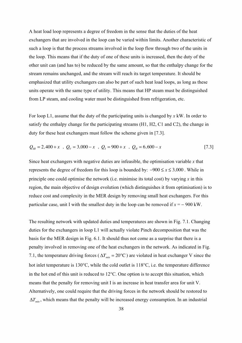
38

A heat load loop represents a degree of freedom in the sense that the duties of the heat

exchangers that are involved in the loop can be varied within limits. Another characteristic of

such a loop is that the process streams involved in the loop flow through two of the units in

the loop. This means that if the duty of one of these units is increased, then the duty of the

other unit can (and has to) be reduced by the same amount, so that the enthalpy change for the

stream remains unchanged, and the stream will reach its target temperature. It should be

emphasized that utility exchangers can also be part of such heat load loops, as long as these

units operate with the same type of utility. This means that HP steam must be distinguished

from LP steam, and cooling water must be distinguished from refrigeration, etc.

For loop L1, assume that the duty of the participating units is changed by x kW. In order to

satisfy the enthalpy change for the participating streams (H1, H2, C1 and C2), the change in

duty for these heat exchangers must follow the scheme given in [7.3].

QIII = 2,400 + x , QV = 3,000 − x , QI = 900 + x , QII = 6,600 − x [7.3]

Since heat exchangers with negative duties are infeasible, the optimisation variable x that

represents the degree of freedom for this loop is bounded by: −900 ≤ x ≤ 3,000 . While in

principle one could optimise the network (i.e. minimise its total cost) by varying x in this

region, the main objective of design evolution (which distinguishes it from optimisation) is to

reduce cost and complexity in the MER design by removing small heat exchangers. For this

particular case, unit I with the smallest duty in the loop can be removed if x = − 900 kW.

The resulting network with updated duties and temperatures are shown in Fig. 7.1. Changing

duties for the exchangers in loop L1 will actually violate Pinch decomposition that was the

basis for the MER design in Fig. 6.1. It should thus not come as a surprise that there is a

penalty involved in removing one of the heat exchangers in the network. As indicated in Fig.

7.1, the temperature driving forces ( ) are violated in heat exchanger V since the

hot inlet temperature is 130°C, while the cold outlet is 118°C, i.e. the temperature difference

in the hot end of this unit is reduced to 12°C. One option is to accept this situation, which

means that the penalty for removing unit I is an increase in heat transfer area for unit V.

Alternatively, one could require that the driving forces in the network should be restored to

, which means that the penalty will be increased energy consumption. In an industrial

ΔTmin = 20°C

ΔTmin

39

setting, the penalty will be split into some additional heat transfer area and some additional

external heating and cooling, dictated by the trade-off between capital cost and operating cost.

For illustration purposes in this case, a heat load path from hot utility to cold utility will be

used to restore the temperature driving forces. The selected path must affect the heat

exchanger with too small in such a way that the driving forces will be restored.

Figure 7.1 Evolved Network for the Illustrative Example

For the network in Fig. 7.1, there is only one heat load path:

(P1): ST → (Ha) → C1 → (V) → H2 → (C) → CW

It should be obvious that more steam and cooling water must be used to restore the driving

forces. This is in line with the Composite Curves in Fig. 4.2, where increased external heating

and cooling will move the two curves apart and increase the temperature driving forces. The

change in duty for the units in the heat load path should follow the scheme given in [7.4].

QHa = 100 + y , QV = 3,900 − y , QC = 3,300 + y [7.4]

The hot inlet temperature to heat exchanger V will remain at 130°C, which means that the

cold outlet temperature must be reduced to 110°C to restore for this unit. This

ΔT

CP (kW/°C) 100 90 ”∞” 50 150 ”∞”

C1

C2

REB

H1

H2

CON

220°C

130°C

150°C

150°C

130°C 130°C

120°C 120°C

50°C

130°C

40°C

80°C

III

III

II

II

Ha

Hb

IV

IV

V

V C

205°C

7,500

1,500 100

3,000

3,000

3,900

3,300

86.7°C

118°C 148°C

100°C

ΔTmin

40

observation will determine the minimum value of the energy penalty y. By following cold

stream C1 through heat exchanger V, the relation in [7.5] can be established.

40 + 3,900 − y( )50

= 110 ⇒ y = 400 kW [7.5]

This means that the energy penalty for removing a heat exchanger with duty x = 900 kW is

considerably less, i.e. y = 400 kW. The general relation between x and y is given by [7.6].

[7.6]

The fact that y < x for the example above can be explained as follows: When unit V (a Pinch

exchanger) is increased in duty from 3,000 to 3,900 kW, both the hot inlet and the cold outlet

temperatures are changed (increased). This means that the duty of this heat exchanger does

not have to be reduced to its original value of 3,000 kW in order to restore the driving forces.

The resulting network (Design A) has the same structure as the design in Fig. 7.1 and will not

be shown here. The units in the heat load path ([7.4]) will have their duties changed by 400

kW, with corresponding changes of the internal network temperatures for streams H2 and C1.

While the initial MER network typically is designed under stringent conditions of Pinch

decomposition and for all heat exchangers, the design evolution stage allows for

relaxation and creative solutions. One should also keep in mind the distinction between hard

and soft stream data discussed in Section 3.2. In the MER network in Fig. 6.1, there is a very

small steam heater with a duty of only 100 kW in order to increase the temperature of cold

stream C1 from 148°C to 150°C. If there is some “softness” in the target temperature for C1,

then this heater should not be installed, and one would accept 148°C as the modified target

temperature for C1. If the original target temperature of 150°C is a hard specification, then

this temperature can still be reached without installing such a small heater. The clue to this

rather creative solution is to use the heat load path P1 in the “opposite” direction (see [7.7]) to

remove the small heater Ha rather than to use heat load loop L1 to remove heat exchanger I.

QHa = 100 − y , QV = 3,000 + y , QC = 3,300 − y [7.7]

0 < y ≤ x

ΔT ≥ ΔTmin

41

By choosing y = 100 kW, the resulting network uses 100 kW less steam and cooling water

and it has one unit less than the MER design. Of course, this does not come without a penalty,

and in the final network for this alternative (Design B) shown in Fig. 7.2, heat exchanger V

has a temperature difference of 18°C in the hot end, which is a very small violation of .

Figure 7.2 An Alternative Network (Design B) for the Illustrative Example

Finally, when removing both heat exchangers I and heater Ha from the initial MER design, it

is not possible to restore in the network, since there is no heat load path. The only

violation in this case is again heat exchanger V that has a temperature difference of

10°C in the hot end. This design is referred to as Design C and is shown together with the

other network alternatives in Table 7.1. While focus in Table 7.1 is on violation in heat

exchanger V, it should not be forgotten that the driving forces for some of the other heat

exchangers in the network are also affected, but these effects are marginal for this particular

example, and there are no other units that violate the specification.

In summary, even for very small processes (as in Fig. 4.1), there are a large number of

different heat exchanger networks that can be designed, with differences both in network

ΔTmin

CP (kW/°C) 100 90 ”∞” 50 150 ”∞”

C1

C2

REB

H1

H2

CON

220°C

130°C

150°C

150°C

130°C 130°C

120°C 120°C

50°C

130°C

40°C

80°C

III

III

II

II I

I

Hb

IV

IV

V

V C

196°C

900 6,600

2,400

3,000

3,000

3,100

3,200

120°C 85.6°C

102°C

100°C 106°C

ΔTmin

ΔTmin

ΔTmin

ΔTmin

42

topology and network parameters (stream temperatures and heat transfer area for the heat

exchangers).

Table 7.1 Alternative Networks for the Simple Process in Fig. 4.1

Design QH (kW) QC (kW) Units ΔTV (°C)

MER 3,100 3,300 8 20

A 3,500 3,700 7 20

B 3,000 3,200 7 18

C 3,000 3,200 6 10

8 Concluding Remarks

In this chapter, the main concepts, representations, procedures and graphical diagrams of

basic Pinch Analysis for Heat Integration have been defined and illustrated with application to

a small and simple process example. The most important topics covered in this chapter are:

• Data Extraction and Process Modifications

• Plus/Minus Principle, Appropriate Placement and Correct Integration

• Performance Targets for Heating, Cooling and Number of Units

• Heat Recovery Pinch and Pinch Decomposition

• Composite Curves, Heat Cascade and Grand Composite Curve

• Grid Diagram and Pinch Design Method with Matching Rules

• Design Evolution with Heat Load Loops and Paths

• Differences between Grassroots and Retrofit Design

The treatment of the topics in this chapter has been kept on a fairly simple level to convey the

most important concepts and provide insight and understanding that will hopefully make the

reading of the other chapters in the Handbook easier. For more reading material on these

topics, readers are referred to textbooks published over the last 15 years by Shenoy (1995),

Smith (2005), Kemp (2007) and Klemeš et al. (2010). Each book provides the state-of-the-art

until the year when it was published.

43

For a more detailed and advanced approach to Heat Integration with focus on Heat Exchanger

Network Design for both Grassroots cases and Retrofit projects, readers are referred to

Chapter 2.5. A number of issues will be discussed and described in Chapter 2.5 that will add

industrial realism to the material. Examples of topics that will be treated are Targets for Heat

Transfer Area and Total Annual Cost, Multiple Utilities, Forbidden Matches, different Heat

Exchanger Types and a brief introduction to the use of Optimisation in Heat Integration. The

different stages in Retrofit Design of heat recovery systems will also be described.

9 Sources of further Information

The primary objective of this chapter has been to introduce the basics of Pinch Analysis as a

foundation and core technology in the discipline of Process Integration. For further and more

detailed information, the reader is advised to consult Chapter 2.5 on Grassroots and Retrofit

Analysis and Design as well as all the other chapters of this Handbook.

References

AspenTech (2009) Aspen Energy Analyser – Reference Guide, <http://www.aspentech.com> accessed 16.08.2012.

CANMET Energy Technology Centre (2003) Pinch Analysis: For the Efficient Use of Energy, Water and Hydrogen, ISBN: 0-662-34964-4, <http://cetc-varennes.nrcan.gc.ca> accessed 12.08.2012.

Gundersen, T. (2000) A Process Integration Primer, IEA Report, SINTEF Energy Research, Trondheim, Norway.

Hohmann, E.C. (1971) Optimum networks for heat exchange, PhD Thesis, University of Southern California, Los Angeles, USA.

Huang, F., Elshout, R.V. (1976) Optimizing the heat recovery of crude units, Chem. Engng. Progr., 72, 68-74.

Kemp, I.C. (2007) Pinch Analysis and Process Integration, 2nd edition, Butterworth-Heinemann (Elsevier), Oxford, UK (authors of the first edition: Linnhoff, B., Townsend, D.W., Boland, D., Hewitt, G.F., Thomas, B.E.A., Guy, A.R., Marsland, R.H. (1982 and 1994) A User guide on process integration for the efficient use of energy, IchemE, Rugby, UK).

Klemeš, J., Friedler, F., Bulatov, I., Varbanov, P. (2010) Sustainability in the process industry – Integration and optimization, McGraw-Hill, New York, USA.

Linnhoff, B. (1979) Thermodynamic analysis in the design of process networks, PhD Thesis, University of Leeds, UK.

44

Linnhoff, B., Dunford, H., Smith, R. (1983) Heat integration of distillation columns into overall processes, Chem. Engng. Sci., 38, 1175-1188.

Linnhoff, B., Flower, J.R. (1978) Synthesis of heat exchanger networks: I. Systematic generation of energy optimal networks, AIChE Jl., 24, 633-642.

Linnhoff, B., Hindmarsh, E. (1983) The pinch design method for heat exchanger networks, Chem. Eng. Sci., 38, 745-763.

Linnhoff March Ltd. (1998) Introduction to Pinch Technology. Linnhoff March Ltd. now part of KBC Advanced Technologies plc., UK.

Linnhoff, B., Mason, D.R., Wardle, I. (1979) Understanding heat exchanger networks, Comput. Chem. Engng., 3, 295-302.

Linnhoff, B., Parker, S. (1984) Heat exchanger networks with process modification, IChemE Annl. Res. Mtg., Bath, UK.

Linnhoff, B., Townsend, D.W. (1982) Designing total energy systems, Chem. Engng. Progr., 78, 72-80.

Linnhoff, B., Townsend, D.W., Boland, D., Hewitt, G.F., Thomas, B.E.A., Guy, A.R., Marsland, R.H. (1982) A User guide on process integration for the efficient use of energy, first edition, IChemE, Rugby, UK. Revised edition 1994.

Linnhoff, B., Turner, J.A. (1981) Heat-recovery networks: new insights yield big savings, Chem. Engng., 88, 56-70.

Linnhoff, B., Vredeveld, D.R. (1984) Pinch Technology has come of age, Chem. Engng. Progr., 80, 33-40.

Shenoy U.V. (1995) Heat exchanger network synthesis – Process optimization by energy and resource analysis, Gulf Publishing, Houston, USA.

Smith, R. (2005) Chemical Process Design and Integration, John Wiley & Sons, Chichester, West Sussex, UK.

Smith, R., Linnhoff, B. (1988) The design of separators in the context of overall processes, Chem. Eng. Res. Des., 66, 195-228.

Umeda, T., Itoh, J., Shiroko, K. (1978) Heat exchange system synthesis, Chem. Engng. Progr., 74, 70-76.

Umeda, T., Niida, K., Shiroko, K. (1979) A thermodynamic approach to heat integration in distillation systems, AIChE Jl., 25, 423-429.