chapter 23: foundations - freefreeit.free.fr/the civil engineering handbook,2003/0958 ch23.pdf ·...

23Foundations

23.1 Effective Stress

23.2 Settlement of FoundationsTime-Dependent Settlement • Magnitude of Acceptable Settlement

23.3 Bearing Capacity of Shallow Foundations

23.4 Pile FoundationsShaft Resistance • Toe Resistance • Ultimate Resistance — Capacity • Critical Depth • Effect of Installation • Residual Load • Analysis of Capacity for Tapered Piles • Factor of Safety • Empirical Methods for Determining Axial Pile Capacity • The Lambda Method • Field Testing for Determining Axial Pile Capacity • Interpretation of Failure Load • Influence of Errors • Dynamic Analysis and Testing • Pile Group Example: Axial Design • Summary of Axial Design of Piles • Design of Piles for Horizontal Loading • Seismic Design of Lateral Pile Behavior

Before a foundation design can be undertaken, the associated soil profile must be well established. Thesoil profile is compiled from three cornerstones of information: borehole records with laboratory clas-sification and testing, piezometer observations, and assessment of the overall geology at the site. Projectswhere construction difficulties, disputes, and litigation arise often have one thing in common: Copies ofborehole field records were thought to determine the soil profile.

An essential part of the foundation design is to come up with a foundation type and size which willhave acceptable values of deformation (settlement) and an adequate margin of safety to failure (the degreeof engaging the soil strength). Deformation is a function of change of effective stress, and soil strengthis proportional to effective stress. Therefore, all applications of foundation design start with determiningthe effective stress distribution of the soil around and below the foundation unit. The distribution thenserves as basis for the design analysis.

23.1 Effective Stress

Effective stress is the total stress minus the pore pressure (the water pressure in the voids). The commonmethod of calculating the effective stress, Ds ¢, contributed by a soil layer is to multiply the buoyant unitweight, g ¢, of the soil with the layer thickness, Dh. Usually, the buoyant unit weight is determined as thebulk unit weight of the soil, gt , minus the unit weight of water, gw , which presupposes that there is novertical gradient of water flow in the soil.

(23.1a)

The effective stress at a depth, s ¢z , is the sum of the contributions from the soil layers above.

s ¢D g ¢ hD=

Bengt H. FelleniusUniversity of Ottawa

© 2003 by CRC Press LLC

23

-2

The Civil Engineering Handbook, Second Edition

(23.1b)

However, most sites display vertical water gradients: either an upward flow, maybe even artesian (thehead is greater than the depth from the ground surface), or a downward flow, and the buoyant unitweight is a function of the gradient, i, in the soil, as follows.

(23.1c)

The gradient is defined as the difference in head between two points divided by the distance the waterhas to flow between these two points. Upward flow gradient is negative and downward flow is positive.For example, if for a particular case of artesian condition the gradient is nearly equal to –1, then, thebuoyant weight is nearly zero. Therefore, the effective stress is close to zero, too, and the soil has little orno strength. This is the case of so-called quicksand, which is not a particular type of sand, but a soil,usually a silty fine sand, subjected to a particular pore pressure condition.

The gradient in a nonhydrostatic condition is often awkward to determine. However, the difficultycan be avoided, because the effective stress is most easily determined by calculating the total stress andthe pore water pressure separately. The effective stress is then obtained by simple subtraction of the latterfrom the former.

Note the difference in terminology — effective stress and pore pressure — which reflects the funda-mental difference between forces in soil as opposed to in water. Soil stress is directional; that is, the stresschanges depending on the orientation of the plane of action in the soil. In contrast, water pressure isomnidirectional, that is, independent of the orientation of the plane. The soil stress and water pressuresare determined, as follows.

The total vertical stress (symbol sz) at a point in the soil profile (also called total overburden stress) iscalculated as the stress exerted by a soil column with a certain weight, or bulk unit weight, and height(or the sum of separate values where the soil profile is made up of a series of separate soil layers havingdifferent bulk unit weights). The symbol for bulk unit weight is gt (the subscript t stands for “total,”because the bulk unit weight is also called total unit weight).

(23.2)

or

Similarly, the pore pressure (symbol u), if measured in a stand-pipe, is equal to the unit weight ofwater, gw , times the height of the water column, h, in the stand-pipe. (If the pore pressure is measureddirectly, the head of water is equal to the pressure divided by the unit weight of water, gw .)

(23.3)

The height of the column of water (the head) representing the water pressure is rarely the distance tothe ground surface or, even, to the groundwater table. For this reason, the height is usually referred toas the phreatic height or the piezometric height to separate it from the depth below the groundwater tableor depth below the ground surface.

The groundwater table is defined as the uppermost level of zero pore pressure. Notice that the soilcan be saturated with water also above the groundwater table without pore pressure being greater thanzero. Actually, because of capillary action, pore pressures in the partially saturated zone above thegroundwater table may be negative.

The pore pressure distribution is determined by applying that (in stationary situations) the porepressure distribution is linear in each individual soil layer, and, in pervious soil layers that are “sand-wiched” between less pervious layers, the pore pressure is hydrostatic (that is, the vertical gradient is zero).

s ¢z S g ¢ hD( )=

g ¢ g t g w 1 i–( )–=

sz g t z=

sz S szD S g t hD( )= =

u g wh=


Foundations

23

-3

The effective overburden stress (symbol s ¢z ) is then obtained as the difference between total stress andpore pressure.

(23.4)

Usually, the geotechnical engineer provides the density (symbol r) instead of unit weight, g. The unitweight is then the density times the gravitational constant, g. (For most foundation engineering purposes,the gravitational constant can be taken to be 10 m/s2 rather than the overly exact value of 9.81 m/s2.)

(23.5)

Many soil reports do not indicate the total soil density, r t , only water content, w, and dry density, r ¢d .For saturated soils, the total density can then be calculated as

(23.6)

The principles of effective stress calculation are illustrated by the calculations involved in the followingsoil profile: an upper 4 m thick layer of normally consolidated sandy silt, 17 m of soft, compressible, slightlyoverconsolidated clay, followed by 6 m of medium dense silty sand and a thick deposit of medium denseto very dense sandy ablation glacial till. The groundwater table lies at a depth of 1.0 m. For originalconditions, the pore pressure is hydrostatically distributed throughout the soil profile. For final conditions,the pore pressure in the sand is not hydrostatically distributed, but artesian with a phreatic height aboveground of 5 m, which means that the pore pressure in the clay is non-hydrostatic (but linear, assumingthat the final condition is long term). The pore pressure in the glacial till is also hydrostatically distributed.A 1.5 m thick earth fill is to be placed over a square area with a 36 m side. The densities of the four soillayers and the earth fill are: 2000 kg/m3, 1700 kg/m3, 2100 kg/m3, 2200 kg/m3, and 2000 kg/m3, respectively.

Calculate the distribution of total and effective stresses as well as pore pressure underneath the centerof the earth fill before and after placing the earth fill. Distribute the earth fill by means of the 2:1 method;that is, distribute the load from the fill area evenly over an area that increases in width and length by anamount equal to the depth below the base of the fill area.

Table 23.1 presents the results of the stress calculation for the example conditions. The calculationshave been made with the Unisettle program [Goudreault and Fellenius, 1993] and the results are presentedin the format of a “hand calculation” to ease verifying the computer calculations. Notice that performingthe calculations at every meter depth is normally not necessary. The table includes a comparison betweenthe non-hydrostatic pore pressure values and the hydrostatic, as well as the effect of the earth fill, whichcan be seen from the difference in the values of total stress for original and final conditions.

The stress distribution below the center of the loaded area was calculated by means of the 2:1 method.However, the 2:1 method is rather approximate and limited in use. Compare, for example, the verticalstress below a loaded footing that is either a square or a circle with a side or diameter of B. For the samecontact stress, q0 , the 2:1 method, strictly applied to the side and diameter values, indicates that thevertical distributions of stress, [qz = q0/(B + z)2], are equal for the square and the circular footings. Yet,the total applied load on the square footing is 4/p = 1.27 times larger than the total load on the circularfooting. Therefore, if applying the 2:1 method to circles and other non-rectangular areas, they should bemodeled as a rectangle of an equal size (“equivalent”) area. Thus, a circle is modeled as an equivalentsquare with a side equal to the circle radius times .

More important, the 2:1 method is inappropriate to use for determining the stress distribution alonga vertical line below a point at any other location than the center of the loaded area. For this reason, itcan not be used to combine stress from two or more loaded areas unless the areas have the same center.To calculate the stresses induced from more than one loaded area and/or below an off-center location,more elaborate methods, such as the Boussinesq distribution (Chapter 20) are required.

A footing is usually placed in an excavation and fill is often placed next to the footing. When calculatingthe stress increase from one or more footing loads, the changes in effective stress from the excavations

s ¢z sz uz– g tz g wh–= =

g rg=

rt rd 1 w+( )=

p


23-4 The Civil Engineering Handbook, Second Edition

and fills must be included which therefore precludes the use of the 2:1 method (unless all such excavationsand fills surround and are concentric with the footing).

A small diameter footing, of about 1 meter width, can normally be assumed to distribute the stressevenly over the footing contact area. However, this cannot be assumed to be the case for wider footings.The Boussinesq distribution assumes ideally flexible footings (and ideally elastic soil). Kany [1959]showed that below a so-called characteristic point, the vertical stress distribution is equal for flexible

TABLE 23.1 Stress Distribution (2:1 Method) at Center of Earth Fill

Original Condition (no earth fill) Final Condition (with earth fill)

Depth st u s ¢ st u s ¢(m) (kPa) (kPa) (kPa) (kPa) (kPa) (kPa)

Layer 1 Sandy Silt r = 2000 kg/m3

0.00 0.0 0.0 0.0 30.0 0.0 30.01.00(GWT) 20.0 0.0 20.0 48.4 0.0 48.42.00 40.0 10.0 30.0 66.9 10.0 56.93.00 60.0 20.0 40.0 85.6 20.0 65.64.00 80.0 30.0 50.0 104.3 30.0 74.3

Layer 2 Soft Clay r = 1700 kg/m3

4.00 80.0 30.0 50.0 104.3 30.0 74.35.00 97.0 40.0 57.0 120.1 43.5 76.66.00 114.0 50.0 64.0 136.0 57.1 79.07.00 131.0 60.0 71.0 152.0 70.6 81.48.00 148.0 70.0 78.0 168.1 84.1 84.09.00 165.0 80.0 85.0 184.2 97.6 86.6

10.00 182.0 90.0 92.0 200.4 111.2 89.211.00 199.0 100.0 99.0 216.6 124.7 91.912.00 216.0 110.0 106.0 232.9 138.2 94.613.00 233.0 120.0 113.0 249.2 151.8 97.414.00 250.0 130.0 120.0 265.6 165.3 100.315.00 267.0 140.0 127.0 281.9 178.8 103.116.00 284.0 150.0 134.0 298.4 192.4 106.017.00 301.0 160.0 141.0 314.8 205.9 109.018.00 318.0 170.0 148.0 331.3 219.4 111.919.00 335.0 180.0 155.0 347.9 232.9 114.920.00 352.0 190.0 162.0 364.4 246.5 117.921.00 369.0 200.0 169.0 381.0 260.0 121.0

Layer 3 Silty Sand r = 2100 kg/m3

21.00 369.0 200.0 169.0 381.0 260.0 121.022.00 390.0 210.0 180.0 401.6 270.0 131.623.00 411.0 220.0 191.0 422.2 280.0 142.224.00 432.0 230.0 202.0 442.8 290.0 152.825.00 453.0 240.0 213.0 463.4 300.0 163.426.00 474.0 250.0 224.0 484.1 310.0 174.127.00 495.0 260.0 235.0 504.8 320.0 184.8

Layer 4 Ablation Till r = 2200 kg/m3

27.00 495.0 260.0 235.0 504.8 320.0 184.828.00 517.0 270.0 247.0 526.5 330.0 196.529.00 539.0 280.0 259.0 548.2 340.0 208.230.00 561.0 290.0 271.0 569.9 350.0 219.931.00 583.0 300.0 283.0 591.7 360.0 231.732.00 605.0 310.0 295.0 613.4 370.0 243.433.00 627.0 320.0 307.0 635.2 380.0 255.2

Note: Calculations by means of UNISETTLE.


Foundations 23-5

and stiff footings. The characteristic point is located at a distance of 0.37B and 0.37L from the centerof a rectangular footing of sides B and L and at a radius of 0.37R from the center of a circular footingof radius R. When applying Boussinesq method of stress distribution to regularly shaped footings, thestress below this point is normally used rather than the stress below the center of the footing.

Calculation of the stress distribution below a point within or outside the footprint of a footing bymeans of the Boussinesq method is time-consuming, in particular if the stress from several loaded areasare to be combined. The geotechnical profession has for many years simplified the calculation effort byusing nomograms over “influence values for vertical stress” at certain locations within the footprint ofa footing. The Newmark influence chart [Newmark, 1935, 1942] is a classic. The calculations are stillrather time consuming. However, since the advent of the computer, several computer programs areavailable which greatly simplify and speed up the calculation effort — for example, Unisettle by Gou-dreault and Fellenius [1993].

23.2 Settlement of Foundations

A foundation is a constructed unit that transfers the load from a superstructure to the ground. Withregard to vertical loads, most foundations receive a more or less concentrated load from the structureand transfer this load to the soil underneath the foundation, distributing the load as a stress over a certainarea. Part of the soil structure interaction is then the condition that the stress must not give rise to adeformation of the soil in excess of what the superstructure can tolerate.

The amount of deformation for a given contact stress depends on the distribution of the stress overthe affected soil mass in relation to the existing stress (the imposed change of effective stress) and thecompressibility of the soil layer. The change of effective stress is the difference between the initial (original)effective stress and the final effective stress, as illustrated in Table 23.1. The stress distribution has beendiscussed in the foregoing. The compressibility of the soil mass can be expressed in either simple orcomplex terms. For simple cases, the soil can be assumed to have a linear stress–strain behavior and thecompressibility can be expressed by an elastic modulus.

Linear stress–strain behavior follows Hooke’s law:

(23.7)

where e = induced strain in a soil layerDs ¢ = imposed change of effective stress in the soil layer

E = elastic modulus of the soil layer

Often the elastic modulus is called Young’s modulus. Strictly speaking, however, Young’s modulus isthe modulus for when lateral expansion is allowed, which may be the case for soil loaded by a smallfooting, but not when loading a larger area. In the latter case, the lateral expansion is constrained. Theconstrained modulus, D, is larger than the E-modulus. The constrained modulus is also called theoedometer modulus. For ideally elastic soils, the ratio between D and E is:

(23.8)

where n = Poisson’s ratio. For example, for a soil material with a Poisson’s ratio of 0.3, a common value,the constrained modulus is 35% larger than the Young’s modulus. (Notice also that the concrete insidea concrete-filled pipe pile behaves as a constrained material as opposed to the concrete in a concrete pile.Therefore, when analyzing the deformation under load, use the constrained modulus for the former andthe Young’s modulus for the latter.)

The deformation of a soil layer, s, is the strain, e, times the thickness, h, of the layer. The settlement, S,of the foundation is the sum of the deformations of the soil layers below the foundation.

e s ¢DE

---------=

DE----

1 n–( )1 n+( ) 1 2n–( )

-------------------------------------=



(23.9)

However, stress–strain behavior is nonlinear for most soils. The nonlinearity cannot be disregardedwhen analyzing compressible soils, such as silts and clays; that is, the elastic modulus approach is notappropriate for these soils. Nonlinear stress–strain behavior of compressible soils is conventionally mod-eled by Eq. (23.10):

(23.10)

where s ¢0 = original (or initial) effective stresss ¢1 = final effective stressCc = compression index e = void ratio

The compression index and the void ratio parameters Cc and e0 are determined by means of oedometertests in the laboratory.

If the soil is overconsolidated, that is, consolidated to a stress (called “preconsolidation stress”) largerthan the existing effective stress, Eq. (23.10) changes to

(23.11)

where s ¢p = preconsolidation stress and Ccr = recompression index.Thus, in conventional engineering practice of settlement design, two compression parameters need to

be established. This is an inconvenience that can be avoided by characterizing the soil with the ratiosCc/(1 + e0) and Ccr /(1 + e0) as single parameters (usually called compression ratio, CR, and recompressionratio, RR, respectively), but few do. Actually, on surprisingly many occasions, geotechnical engineers onlyreport the Cc parameter — neglecting to include the e0 value — or worse, report the Cc from the oedometertest and the e0 from a different soil specimen than used for determining the compression index! This isnot acceptable, of course. The undesirable challenge of ascertaining what Cc value goes with what e0 valueis removed by using the Janbu tangent modulus approach instead of the Cc and e0 approach, applying amodulus number, m, instead.

The Janbu tangent modulus approach, proposed by Janbu [1963, 1965, 1967] and referenced by theCanadian Foundation Engineering Manual, (CFEM) [Canadian Geotechnical Society, 1985], appliesthe same basic principle of nonlinear stress–strain behavior to all soils, clays as well as sand. By thismethod, the relation between stress and strain is a function of two nondimensional parameters whichare unique for a soil: a stress exponent, j, and a modulus number, m.

In cohesionless soils, j > 0, the following simple formula governs:

(23.12)

where e = strain induced by increase of effective stresss ¢0 = the original effective stresss ¢1 = the final effective stress

j = the stress exponentm = the modulus number, which is determined from laboratory and/or field testing

s ¢r = a reference stress, a constant, which is equal to 100 kPa ( = 1 tsf = 1 kg/cm2)

S sÂ eh( )Â= =

e Cc

1 e0+------------- lg=

s ¢1

s ¢0

--------

e 11 e0+------------- Ccr lg

s ¢p

s ¢0-------- Cc lg

s ¢1

s ¢p

--------+=

e 1mj------ s ¢1

s ¢r

--------Ë ¯Ê ˆ j s ¢0

s ¢r

--------Ë ¯Ê ˆ j

–=


Foundations 23-7

In an essentially cohesionless, sandy or silty soil, the stress exponent is close to a value of 0.5. Byinserting this value and considering that the reference stress is equal to 100 kPa, Eq. (23.12) is simplified to

(23.13a)

Notice that Eq. (23.13a) is not independent of the choice of units; the stress values must be insertedin kPa. That is, a value of 5 MPa is to be inserted as the number 5000 and a value of 300 Pa as the number0.3. In English units, Eq. (23.13a) becomes

(23.13b)

Again, the equation is not independent of units: Because the reference stress converts to 1.0 tsf,Eq. (23.13b) requires that the stress values be inserted in units of tsf.

If the soil is overconsolidated and the final stress exceeds the preconsolidation stress, Eqs. (23.13a)and (23.13b) change to

(23.14a)

(23.14b)

where s ¢0 = original effective stress (kPa or tsf)s ¢p = preconsolidation stress (kPa or tsf)s ¢1 = final effective stress (kPa or tsf)m = modulus number (dimensionless)mr = recompression modulus number (dimensionless)

Equation (23.14a) requires stress units in kPa and Eq. (23.14b) stress units in tsf.If the imposed stress does not result in a new (final) stress that exceeds the preconsolidation stress,

Eqs. (23.13a) and (23.13b) become

(23.15a)

(23.15b)

Equation (23.15a) requires stress units in kPa and Eq. (23.15b) units in tsf.In cohesive soils, the stress exponent is zero, j = 0. Then, in a normally consolidated cohesive soil:

(23.16)

and in an overconsolidated cohesive soil

(23.17)

e 15m------- s ¢1 s ¢0–Ë ¯

Ê ˆ .=

e 2m---- s ¢1 s ¢0–Ë ¯

Ê ˆ .=

e 15mr

--------- s ¢p s ¢0–Ë ¯Ê ˆ 1

5m------- s ¢1 s ¢p–Ë ¯

Ê ˆ+=

e 2mr

------ s ¢p s ¢0–Ë ¯Ê ˆ 2

m---- s ¢1 s ¢p–Ë ¯

Ê ˆ+=

e 15mr

--------- s ¢1 s ¢0–Ë ¯Ê ˆ=

e 2mr

------ s ¢1 s ¢0–Ë ¯Ê ˆ=

e 1m---- ln

s ¢1

s ¢0--------Ë ¯

Ê ˆ=

e 1mr

------ lns ¢ps ¢0-------Ë ¯

Ê ˆ 1m---- ln

s ¢1s ¢p-------Ë ¯

Ê ˆ+=



Notice that the ratio (s ¢p /s ¢0 ) is equal to the overconsolidation ratio, OCR. Of course, the extent ofoverconsolidation may also be expressed as a fixed stress-unit value, s ¢p – s ¢0 .

If the imposed stress does not result in a new stress that exceeds the preconsolidation stress, Eq. (23.17)becomes

(23.18)

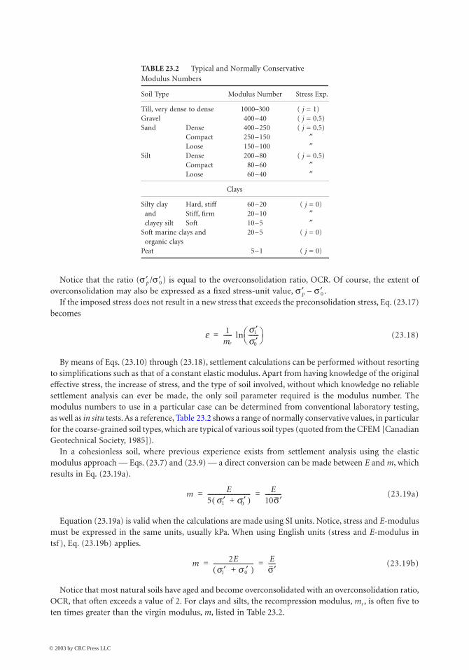
By means of Eqs. (23.10) through (23.18), settlement calculations can be performed without resortingto simplifications such as that of a constant elastic modulus. Apart from having knowledge of the originaleffective stress, the increase of stress, and the type of soil involved, without which knowledge no reliablesettlement analysis can ever be made, the only soil parameter required is the modulus number. Themodulus numbers to use in a particular case can be determined from conventional laboratory testing,as well as in situ tests. As a reference, Table 23.2 shows a range of normally conservative values, in particularfor the coarse-grained soil types, which are typical of various soil types (quoted from the CFEM [CanadianGeotechnical Society, 1985]).

In a cohesionless soil, where previous experience exists from settlement analysis using the elasticmodulus approach — Eqs. (23.7) and (23.9) — a direct conversion can be made between E and m, whichresults in Eq. (23.19a).

(23.19a)

Equation (23.19a) is valid when the calculations are made using SI units. Notice, stress and E-modulusmust be expressed in the same units, usually kPa. When using English units (stress and E-modulus intsf ), Eq. (23.19b) applies.

(23.19b)

Notice that most natural soils have aged and become overconsolidated with an overconsolidation ratio,OCR, that often exceeds a value of 2. For clays and silts, the recompression modulus, mr , is often five toten times greater than the virgin modulus, m, listed in Table 23.2.

TABLE 23.2 Typical and Normally Conservative Modulus Numbers

Soil Type Modulus Number Stress Exp.

Till, very dense to dense 1000–300 ( j = 1)Gravel 400–40 ( j = 0.5)Sand Dense 400–250 ( j = 0.5)

Compact 250–150 ≤Loose 150–100 ≤

Silt Dense 200–80 ( j = 0.5)Compact 80–60 ≤Loose 60–40 ≤

Clays

Silty clay and clayey silt

Hard, stiffStiff, firmSoft

60–2020–1010–5

( j = 0)≤≤

Soft marine clays and organic clays

20–5 ( j = 0)

Peat 5–1 ( j = 0)

e 1mr

------ lns ¢1s ¢0-------Ë ¯

Ê ˆ=

m E5 s ¢1 s ¢+ 0( )----------------------------- E

10s¢-----------= =

m 2Es ¢1 s ¢0+( )

--------------------------- Es¢-----= =


Foundations 23-9

The conventional Cc and e0 method and the Janbu modulus approach are identical in a cohesive soil.A direct conversion factor as given in Eq. (23.20) transfers values of one method to the other.

(23.20)

Designing for settlement of a foundation is a prediction exercise. The quality of the prediction — thatis, the agreement between the calculated and the actual settlement value — depends on how accuratelythe soil profile and stress distributions applied to the analysis represent the site conditions, and howclosely the loads, fills, and excavations considered resemble those actually occurring. The quality dependsalso, of course, on the quality of the soil parameters used as input to the analysis. Soil parameters forcohesive soils depend on the quality of the sampling and laboratory testing. Clay samples tested in thelaboratory should be from carefully obtained “undisturbed” piston samples. Paradoxically, the moredisturbed the sample is, the less compressible the clay appears to be. The error which this could cause isto a degree “compensated for” by the simultaneous apparent reduction in the overconsolidation ratio.Furthermore, high-quality sampling and oedometer tests are costly, which limits the amounts of infor-mation procured for a routine project. The designer usually runs the tests on the “worst” samples andarrives at a conservative prediction. This is acceptable, but only too often is the word “conservative”nothing but a disguise for the more appropriate terms of “erroneous” and “unrepresentative” and theend results may not even be on the “safe side.”

Non-cohesive soils cannot easily be sampled and tested. Therefore, settlement analysis of foundationsin such soils must rely on empirical relations derived from in situ tests and experience values. Usually,these soils are less compressible than cohesive soils and have a more pronounced overconsolidation.However, considering the current tendency toward larger loads and contact stresses, foundation designmust prudently address the settlement expected in these soils as well. Regardless of the methods that areused for prediction of the settlement, it is necessary to refer the results of the analyses back to basics.That is, the settlement values arrived at in the design analysis should be evaluated to indicate whatcorresponding compressibility parameters (Janbu modulus numbers) they represent for the actual soilprofile and conditions of effective stress and load. This effort will provide a check on the reasonablenessof the results as well as assist in building up a reference database for future analyses.

Time-Dependent Settlement

Because soil solids compress very little, settlement is mostly the result of a change of pore volume.Compression of the solids is called initial compression. It occurs quickly and it is usually considered elasticin behavior. In contrast, the change of pore volume will not occur before the water occupying the poresis squeezed out by an increase of stress. The process is rapid in coarse-grained soils and slow in fine-grained soils. In fine clays, the process can take a longer time than the life expectancy of the building,or of the designing engineer, at least. The process is called consolidation and it usually occurs with anincrease of both undrained and drained soil shear strength. By analogy with heat dissipation in solidmaterials, the Terzaghi consolidation theory indicates simple relations for the time required for theconsolidation. The most commonly applied theory builds on the assumption that water is able to drainout of the soil at one surface boundary and not at all at the opposite boundary. The consolidation is fastin the beginning, when the driving pore pressures are greater, and slows down with time. The analysismakes use of the relative amount of consolidation obtained at a certain time, called average degree ofconsolidation, which is defined as follows:

(23.21)

m ln 101 e0+

Cc

-------------Ë ¯Ê ˆ 2.30

1 e0+Cc

-------------Ë ¯Ê ˆ= =

USt

Sf

---- 1 ut

u0

-----–= =



where = average degree of consolidationS t = settlement at time tS f = final settlement at full consolidation

= average pore pressure at time t= initial average pore pressure (on application of the load; time t = 0)

Notice that the pore pressure varies throughout the soil layer and Eq. (23.21) assumes average values.In contrast, the settlement values are not the average, but the accumulated values.

The time for achieving certain degree consolidation is then, as follows:

(23.22)

where t = time to obtain a certain degree of consolidationTv = a dimensionless time coefficientcv = coefficient of consolidationH = length of the longest drainage path

The time coefficient, Tv, is a function of the type of pore pressure distribution. Of course, the shapeof the distribution affects the average pore pressure values and a parabolic shape is usually assumed. Thecoefficient of consolidation is determined in the laboratory oedometer test (some in situ tests can alsoprovide cv values) and it can rarely be obtained more accurately than within a ratio range of 2 or 3. Thelength of the longest drainage path, H, for a soil layer that drains at both surface boundaries is half thelayer thickness. If drainage only occurs at one boundary, H is equal to the full layer thickness. Naturally,in layered soils, the value of H is difficult to ascertain.

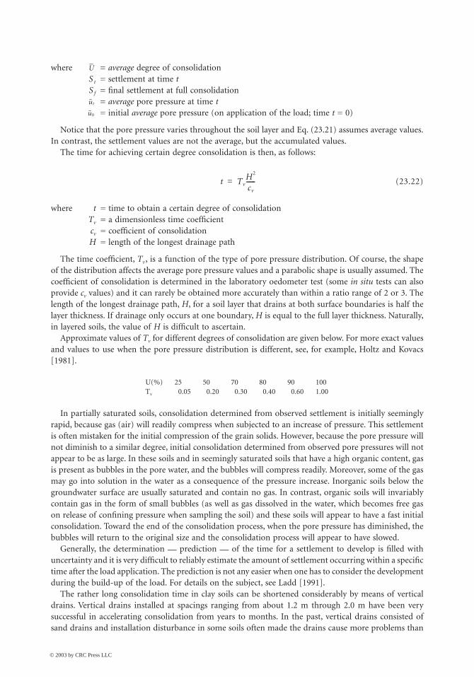
Approximate values of Tv for different degrees of consolidation are given below. For more exact valuesand values to use when the pore pressure distribution is different, see, for example, Holtz and Kovacs[1981].

In partially saturated soils, consolidation determined from observed settlement is initially seeminglyrapid, because gas (air) will readily compress when subjected to an increase of pressure. This settlementis often mistaken for the initial compression of the grain solids. However, because the pore pressure willnot diminish to a similar degree, initial consolidation determined from observed pore pressures will notappear to be as large. In these soils and in seemingly saturated soils that have a high organic content, gasis present as bubbles in the pore water, and the bubbles will compress readily. Moreover, some of the gasmay go into solution in the water as a consequence of the pressure increase. Inorganic soils below thegroundwater surface are usually saturated and contain no gas. In contrast, organic soils will invariablycontain gas in the form of small bubbles (as well as gas dissolved in the water, which becomes free gason release of confining pressure when sampling the soil) and these soils will appear to have a fast initialconsolidation. Toward the end of the consolidation process, when the pore pressure has diminished, thebubbles will return to the original size and the consolidation process will appear to have slowed.

Generally, the determination — prediction — of the time for a settlement to develop is filled withuncertainty and it is very difficult to reliably estimate the amount of settlement occurring within a specifictime after the load application. The prediction is not any easier when one has to consider the developmentduring the build-up of the load. For details on the subject, see Ladd [1991].

The rather long consolidation time in clay soils can be shortened considerably by means of verticaldrains. Vertical drains installed at spacings ranging from about 1.2 m through 2.0 m have been verysuccessful in accelerating consolidation from years to months. In the past, vertical drains consisted ofsand drains and installation disturbance in some soils often made the drains cause more problems than

U(%) 25 50 70 80 90 100Tv 0.05 0.20 0.30 0.40 0.60 1.00

U

ut

u0

t TvH2

cv

------=


Foundations 23-11

they solved. However, the sand drain is now replaced by premanufactured band-shaped drains, wickdrains, which do not share the difficulties and adverse behavior of sand drains.

Theoretically, when vertical drains have been installed, the drainage is in the horizontal direction anddesign formulas have been developed as based on radial drainage. However, vertical drains connecthorizontal layers of greater permeability, which frequently are interspersed in natural soils, which makethe theoretical calculations quite uncertain. Some practical aspects of the use of vertical drains aredescribed in the CFEM [Canadian Geotechnical Society, 1985].

The settlement will continue after the end of the consolidation. This type of settlement is called creepor secondary compression. Creep is a function of a coefficient of secondary compression, Ca , and the ratioof the time considered after full consolidation and the time for full consolidation to develop:

(23.23)

where Ca = coefficient of secondary compressionta = time after end of consolidation

t100 = time for achieving primary compression

In most soils, creep is small in relation to the consolidation settlement and is therefore neglected.However, in organic soils, creep may be substantial.

Magnitude of Acceptable Settlement

For many years, settlement analysis was limited to ascertaining that the expected settlement should notexceed one inch. (Realizing that 25.4 mm is too precise a value — as is 25 mm when transferring thislimit to the SI system — some have argued whether the “metric inch” should be 20 mm or 30 mm).Furthermore, both total settlement and differential settlement must be evaluated. The Canadian Foun-dation Engineering Manual [Canadian Geotechnical Society, 1985] lists allowable displacement criteriain terms of maximum deflection between point supports, maximum slope of continuous structures, androtation limits for structures. The multitude of limits demonstrate clearly that the acceptable settlementvaries with the type and size of structure considered. Moreover, modern structures often have smalltolerance for settlement and, therefore, require a more thorough settlement analysis. The advent of thecomputer and development of sophisticated yet simple to use design software have enabled the structuralengineers to be very precise in the analysis of deformations and the effect of deformations on the stressand strain in various parts of a structure. As a not so surprising consequence, requests for “settlement-free” foundations have increased. When the geotechnical engineer is vague on the predicted settlement,the structural designer “plays it safe” and increases the size of footings or changes the foundation type,which may increase the costs of the structure. These days, in fact, the geotechnical engineer cannot justestimate a “less than one inch” value, but must provide a more accurate value by performing a thoroughanalysis considering soil compressibility, soil layering, and load variations. Moreover, the analysis mustbe put into the context of the structure, which necessitates a continuous communication between thegeotechnical and structural engineers during the design effort. Building codes have started to recognizethe complexity of the problem and mandate that the designers collaborate continuously. See, for example,the 1993 Canadian Highway Bridge Design Code.

23.3 Bearing Capacity of Shallow Foundations

When society started building and imposing large concentrated loads onto the soil, occasionally thestructure would fail catastrophically. Initially, the understanding of foundation behavior progressed fromone failure to the next. Later, tests were run of model footings in different soils and the test results wereextrapolated to the behavior of full-scale foundations. For example, loading tests on model size footings

ecreepCa

1 e0+( )------------------ ln

ta

t100

-------=



in normally consolidated clay showed load-movement curves where the load increased to a distinct peakvalue — bearing capacity failure — indicating that the capacity (not the settlement) of a footing in clayis independent of the footing size.

The behavior of footing in clay differs from the behavior of footings in sand, however. Figure 23.1presents results from loading tests on a 150-mm diameter footing in dry sand of densities varying fromvery dense to loose. In the dense sand, a peak value is evident. In less dense sands, no such peak is found.

The capacity and the load movement of a footing in sand are almost directly proportional to the footingsize. This is illustrated in Fig. 23.2, which shows some recent test results on footings of different size in afine sand. Generally, eccentric loading, inclined loading, footing shape, and foundation depth influencethe behavior of footings. Early on, Terzaghi developed the theoretical explanations to observed behaviorsinto a “full bearing capacity formula,” as given in Eq. (23.24a) and applicable to a continuous footing:

(23.24a)

where ru = ultimate unit resistance of the footingc ¢ = effective cohesion interceptB = footing widthq ¢ = overburden effective stress at the foundation levelg ¢ = average effective unit weight of the soil below the foundation

Nc, Nq, Ng = nondimensional bearing capacity factors

The bearing capacity factors are a function of the effective friction angle of the soil. Such factors werefirst originated by Terzaghi, later modified by Meyerhof, Berezantsev, and others. As presented in theCanadian Foundation Engineering Manual [Canadian Geotechnical Society, 1985], the bearing capacityfactors are somewhat interrelated, as follows.

FIGURE 23.1 Contact stress vs. settlement of 150-mm footings. (Source: Vesic, 1967.)

0

20

40

ST

RE

SS

(ps

i)

ST

RE

SS

(kP

a)

60

80

0.0 0.5 1.0 1.5 2.0

SETTLEMENT

2.5 3.0 (inch)0

100

200

300

400#61, Pd = 96.2 pcf

#62, Pd = 93.0 pcf

#63, Pd = 91.7 pcf

#64, Pd = 85.0 pcf

500

75 (mm)50250

ru c¢Nc q¢ Nq 1–( ) 0.5B g ¢Ng+ +=


Foundations 23-13

(23.24b)

(23.24c)

(23.24d)

For friction angles larger than about 37∞, the bearing capacity factors increase rapidly and theformula loses in relevance.

For a footing of width B subjected to a load Q, the applied contact stress is q (= Q /B) per unit lengthand the applied contact stress mobilizes an equally large soil resistance, r. Of course, the soil resistancecan not exceed the strength of the soil. Equation (23.24a) indicates the maximum available (ultimate)resistance, ru. In the design of a footing for bearing capacity, the applied load is only allowed to reach acertain portion of the ultimate resistance. That is, as is the case for all foundation designs, the designmust include a margin of safety against failure. In most geotechnical applications, this margin is achievedby applying a factor of safety defined as the available soil strength divided by the mobilized shear. Theavailable strength is either cohesion, c, friction, tan j, or both combined. (Notice that friction is not thefriction angle, j, but its tangent, tan j). However, in bearing capacity problems, the factor of safety isusually defined somewhat differently and as given by Eq. (23.24e):

(23.24e)

where Fs = factor of safetyru = ultimate unit resistance (unit bearing capacity)

qallow = the allowable bearing stress

FIGURE 23.2 Stress vs. normalized settlement. (Data from Ismael, 1985.)

2000

1500

1000 B = 0.25 m

B = 0.50 m

B = 0.75 m

B = 1.00 m

ST

RE

SS

(kP

a)

500

00 5 10

SETTLEMENT (%)

15 20

Nq ep j ¢tan( ) 1 j ¢sin+1 j ¢sin–----------------------Ë ¯

Ê ˆ= j¢ 0Æ Nq 1Æ

Nc Nq 1–( ) j¢cot( )= j¢ 0Æ Nc 5.14Æ

Ng 1.5 Nq 1–( ) j¢tan( )= j¢ 0Æ Ng 0Æ

Fs ru qallow§=



The factor of safety applied to the bearing capacity formula is usually recommended to be no smallerthan 3.0, usually equal to 4.0. There is some confusion whether, in the bearing capacity calculatedaccording to Eq. (23.24a), the relation (Nq – 1) should be used in lieu of Nq and, then, whether or notthe allowable bearing stress should be the “net” stress, that is, the value exceeding the existing stress atthe footing base. More importantly, however, is that the definition of factor of safety given by Eq. (23.24e)is not the same as the factor of safety applied to the shear strength, because the ultimate resistancedetermined by the bearing capacity formula includes several aspects other than soil shear strength,particularly so for foundations in soil having a substantial friction component. Depending on the detailsof each case, a value of 3 to 4 for the factor defined by Eq. (23.24e) corresponds, very approximately, toa factor of safety on shear strength in the range of 1.5 through 2.0.

In fact, the bearing capacity formula is wrought with much uncertainty and the factor of safety, be it3 or 4, applied to a bearing capacity formula is really a “factor of ignorance” and does not always guaranteean adequate safety against failure. Therefore, in the design of footings, be it in clays or sands, the settlementanalysis should be given more weight than the bearing capacity formula calculation.

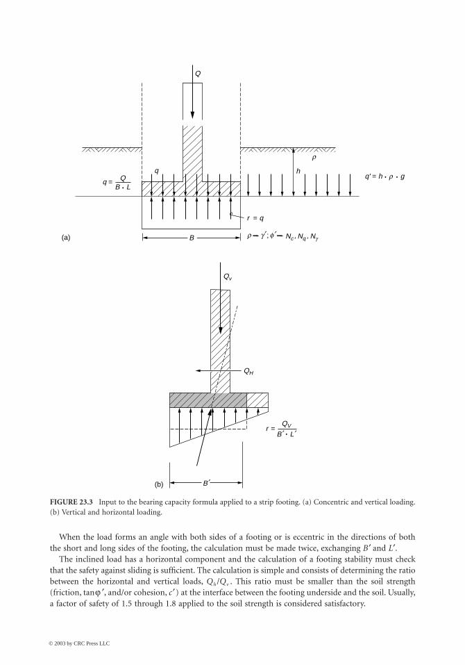
Footings are rarely loaded only vertically and concentrically. Figure 23.3(b) illustrates the general caseof a footing subjected to both inclined and eccentric load. Eq. (23.24a) changes to

(23.24f)

where factors not defined earlier are

sc, sq, sg = nondimensional shape factorsic, iq, ig = nondimensional inclination factors

B¢ = equivalent or effective footing width

The shape factors are

(23.24g)

where L¢ = equivalent or effective footing length.

(23.24h)

The inclination factors are

(23.24i)

(23.24j)

An inclined load can have a significant reducing effect on the bearing capacity of a footing. Directly,first, as reflected by the inclination factor and then also because the resultant to the load on most occasionsacts off center. An off-center load will cause increased stress, edge stress, on one side and a decreasedstress on the opposing side. A large edge stress can be the starting point of a failure. In fact, most footings,when they fail, fail by tilting, which is an indication of excessive edge stress. To reduce the risk for failure,the bearing capacity formula (which assumes a uniform load) applies the term B ¢ in Eq. (23.24f ), theeffective footing width, which is the width of a smaller footing having the resultant load in its center.That is, the calculated ultimate resistance is decreased because of the reduced width (g component) andthe applied stress is increased because it is calculated over the effective area [as q = Q/(B¢/L¢)]. Theapproach is approximate and its application is limited to the requirement that the contact stress mustnot be reduced beyond a zero value at the opposite edge (“No tension at the heel”). This means that theresultant must fall within the middle third of the footing, or the eccentricity must not be greater than B/6.

ru scicc ¢Nc sqiqq¢Nq sg ig 0.5B ¢g ¢Ng+ +=

sc sq 1 B¢ L¢§( ) Nq Nc§( )+= =

sg 1 0.4 B¢ L¢§( )–=

ic iq 1 d 90∞§–( )2= =

ig 1 d j¢§–( )2=


Foundations 23-15

When the load forms an angle with both sides of a footing or is eccentric in the directions of boththe short and long sides of the footing, the calculation must be made twice, exchanging B ¢ and L¢.

The inclined load has a horizontal component and the calculation of a footing stability must checkthat the safety against sliding is sufficient. The calculation is simple and consists of determining the ratiobetween the horizontal and vertical loads, Qh/Qv . This ratio must be smaller than the soil strength(friction, tan j ¢, and/or cohesion, c ¢) at the interface between the footing underside and the soil. Usually,a factor of safety of 1.5 through 1.8 applied to the soil strength is considered satisfactory.

FIGURE 23.3 Input to the bearing capacity formula applied to a strip footing. (a) Concentric and vertical loading.(b) Vertical and horizontal loading.

Q

hqq' = h . r . g

r = q

r

B(a)

(b) B¢�

Nc Nq Ng, ,;r g ¢� f ¢�

q = QB . L

r = QV

B¢ . L¢�

Qv

QH



In summary, the bearing capacity calculation of a footing is governed by the bearing capacity of auniformly loaded equivalent footing, with a check for excessive edge stress (eccentricity) and safety againstsliding. In some texts, an analysis of “overturning” is mentioned, which consists of taking the momentof forces at the edge of the footing and applying a factor of safety to the equilibrium. This is an incorrectapproach, because long before the moment equilibrium has been reached, the footing fails due to excessiveedge stress. (It is also redundant, because the requirement for the resultant to be located within themiddle third takes care of the “overturning.”) In fact, “overturning” failure will occur already at acalculated “factor of safety” as large as about 1.3 on the moment equilibrium. Notice that the factor ofsafety approach absolutely requires that the calculation of the stability of the structure indicates that itis stable also at a factor of safety very close to unity — theoretically stable, that is.

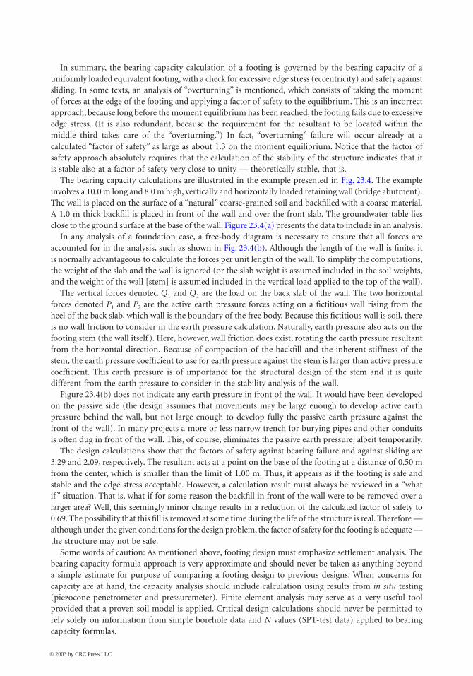
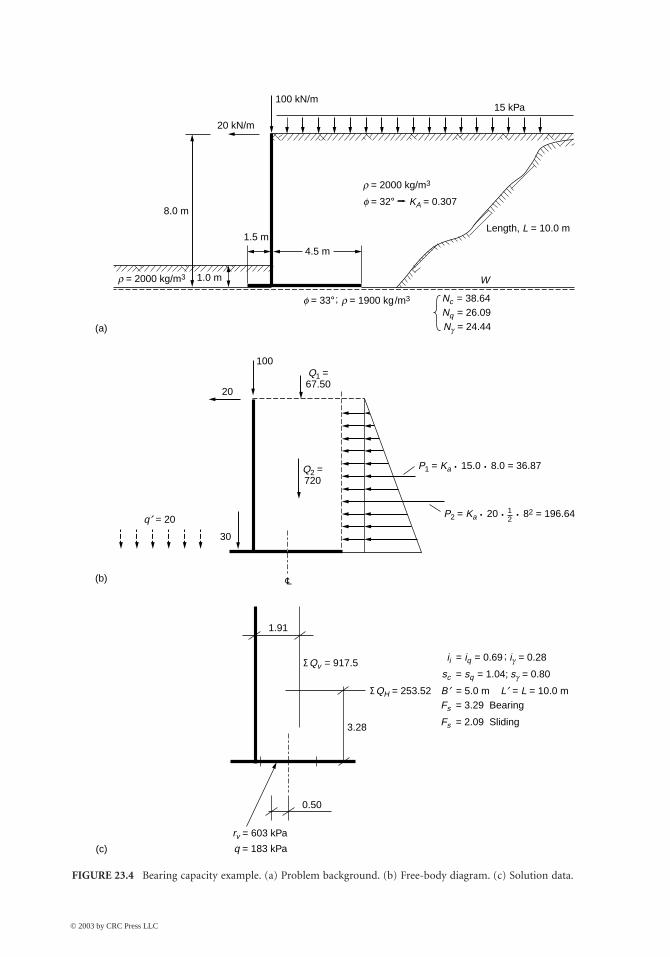
The bearing capacity calculations are illustrated in the example presented in Fig. 23.4. The exampleinvolves a 10.0 m long and 8.0 m high, vertically and horizontally loaded retaining wall (bridge abutment).The wall is placed on the surface of a “natural” coarse-grained soil and backfilled with a coarse material.A 1.0 m thick backfill is placed in front of the wall and over the front slab. The groundwater table liesclose to the ground surface at the base of the wall. Figure 23.4(a) presents the data to include in an analysis.

In any analysis of a foundation case, a free-body diagram is necessary to ensure that all forces areaccounted for in the analysis, such as shown in Fig. 23.4(b). Although the length of the wall is finite, itis normally advantageous to calculate the forces per unit length of the wall. To simplify the computations,the weight of the slab and the wall is ignored (or the slab weight is assumed included in the soil weights,and the weight of the wall [stem] is assumed included in the vertical load applied to the top of the wall).

The vertical forces denoted Q1 and Q2 are the load on the back slab of the wall. The two horizontalforces denoted P1 and P2 are the active earth pressure forces acting on a fictitious wall rising from theheel of the back slab, which wall is the boundary of the free body. Because this fictitious wall is soil, thereis no wall friction to consider in the earth pressure calculation. Naturally, earth pressure also acts on thefooting stem (the wall itself ). Here, however, wall friction does exist, rotating the earth pressure resultantfrom the horizontal direction. Because of compaction of the backfill and the inherent stiffness of thestem, the earth pressure coefficient to use for earth pressure against the stem is larger than active pressurecoefficient. This earth pressure is of importance for the structural design of the stem and it is quitedifferent from the earth pressure to consider in the stability analysis of the wall.

Figure 23.4(b) does not indicate any earth pressure in front of the wall. It would have been developedon the passive side (the design assumes that movements may be large enough to develop active earthpressure behind the wall, but not large enough to develop fully the passive earth pressure against thefront of the wall). In many projects a more or less narrow trench for burying pipes and other conduitsis often dug in front of the wall. This, of course, eliminates the passive earth pressure, albeit temporarily.

The design calculations show that the factors of safety against bearing failure and against sliding are3.29 and 2.09, respectively. The resultant acts at a point on the base of the footing at a distance of 0.50 mfrom the center, which is smaller than the limit of 1.00 m. Thus, it appears as if the footing is safe andstable and the edge stress acceptable. However, a calculation result must always be reviewed in a “whatif ” situation. That is, what if for some reason the backfill in front of the wall were to be removed over alarger area? Well, this seemingly minor change results in a reduction of the calculated factor of safety to0.69. The possibility that this fill is removed at some time during the life of the structure is real. Therefore —although under the given conditions for the design problem, the factor of safety for the footing is adequate —the structure may not be safe.

Some words of caution: As mentioned above, footing design must emphasize settlement analysis. Thebearing capacity formula approach is very approximate and should never be taken as anything beyonda simple estimate for purpose of comparing a footing design to previous designs. When concerns forcapacity are at hand, the capacity analysis should include calculation using results from in situ testing(piezocone penetrometer and pressuremeter). Finite element analysis may serve as a very useful toolprovided that a proven soil model is applied. Critical design calculations should never be permitted torely solely on information from simple borehole data and N values (SPT-test data) applied to bearingcapacity formulas.


Foundations 23-17

FIGURE 23.4 Bearing capacity example. (a) Problem background. (b) Free-body diagram. (c) Solution data.

(a)

(b)

(c)

100 kN/m

20 kN/m

15 kPa

4.5 m

100

20

30

1.91

0.50

3.28

1.5 m

W

Length, L = 10.0 m

1.0 m

8.0 m

r = 2000 kg/m3

f = 32° KA = 0.307

r = 2000 kg/m3

Nc = 38.64Nq = 26.09Ng = 24.44

Q1 =67.50

P1 = Ka . 15.0 . 8.0 = 36.87

q¢ = 20 P2 = Ka . 20 . . 82 = 196.64

rv = 603 kPa

q = 183 kPa

Q2 =720

f = 33° r = 1900 kg/m3;

cL

12

ΣQv = 917.5

ΣQH = 253.52

sc = sq = 1.04; sg = 0.80

Fs = 3.29 Bearing

Fs = 2.09 Sliding

B¢ = 5.0 m L¢ = L = 10.0 m

ii = iq = 0.69 ig = 0.28;



23.4 Pile Foundations

Where using shallow foundations would mean unacceptable settlement, or where scour and other envi-ronmental risks exist which could impair the structure in the future, deep foundations are used. Deepfoundations usually consist of piles, which are slender structural units installed by driving or by in situconstruction methods through soft compressible soil layers into competent soils. Piles can be made ofwood, concrete, or steel, or be composite, such as concrete-filled steel pipes or an upper concrete sectionconnected to a lower steel or wood section. They can be round, square, hexagonal, octagonal, even triangularin shape, and straight shafted, step tapered, or conical. In order to arrive at a reliable design, the particularsof the pile must be considered, most important, the pile material and the method of construction.

Pile foundation design starts with an analysis of how the load applied to the pile head is transferredto the soil. This analysis is the basis for a settlement analysis, because in contrast to the design of shallowfoundations, settlement analysis of piles cannot be separated from a load-transfer analysis. The load-transfer analysis is often called static analysis or capacity analysis. Total stress analysis using undrainedshear strength (so-called a-method) has very limited application, because the load transfer between apile and the soil is governed by effective stress behavior. In an effective stress analysis (also calledb-method), the resistance is proportional to the effective overburden stress. Sometimes, an adhesion(cohesion) component is added. (The adhesion component is normally not applicable to driven piles,but may be useful for cast in situ piles). The total stress and effective stress approaches refer to both shaftand toe resistances, although the equivalent terms, “a-method” and “b-method” usually refer to shaftresistance, specifically.

Shaft Resistance

The general numerical relation for the unit shaft resistance, rs, is

(23.25a)

The adhesion component, c¢, is normally set to zero for driven piles and Eq. (23.25a) then expressesthat unit shaft resistance is directly proportional to the effective overburden stress.

The accumulated (total) shaft resistance, Rs, is

(23.25b)

The beta coefficient varies with soil gradation, mineralogical com-position, density, and soil strength within a fairly narrow range.Table 23.3 shows the approximate range of values to expect from basicsoil types.

Toe Resistance

Also the unit toe resistance, rt , is proportional to the effective stress,that is, the effective stress at the pile toe (z = D). The proportionalitycoefficient has the symbol Nt . Its value is sometimes stated to be ofsome relation to the conventional bearing capacity coefficient, Nq, butsuch relation is far from strict. The toe resistance, rt, is

(23.26a)

The total toe resistance, Rt, acting on a pile with a toe area equal to At is

(23.26b)

rs c ¢ bs ¢z+=

Rs Asrs zdÚ As c ¢ bs ¢z+( ) zdÚ= =

TABLE 23.3 Approximate Range of Beta Coefficients

Soil Type Phi Beta

Clay 25-30 0.25-0.35Silt 28-34 0.27-0.50Sand 32-40 0.30-0.60Gravel 35-45 0.35-0.80

rt Nt s ¢z D= .=

Rt Atrt At Nt s ¢z D= .= =


Foundations 23-19

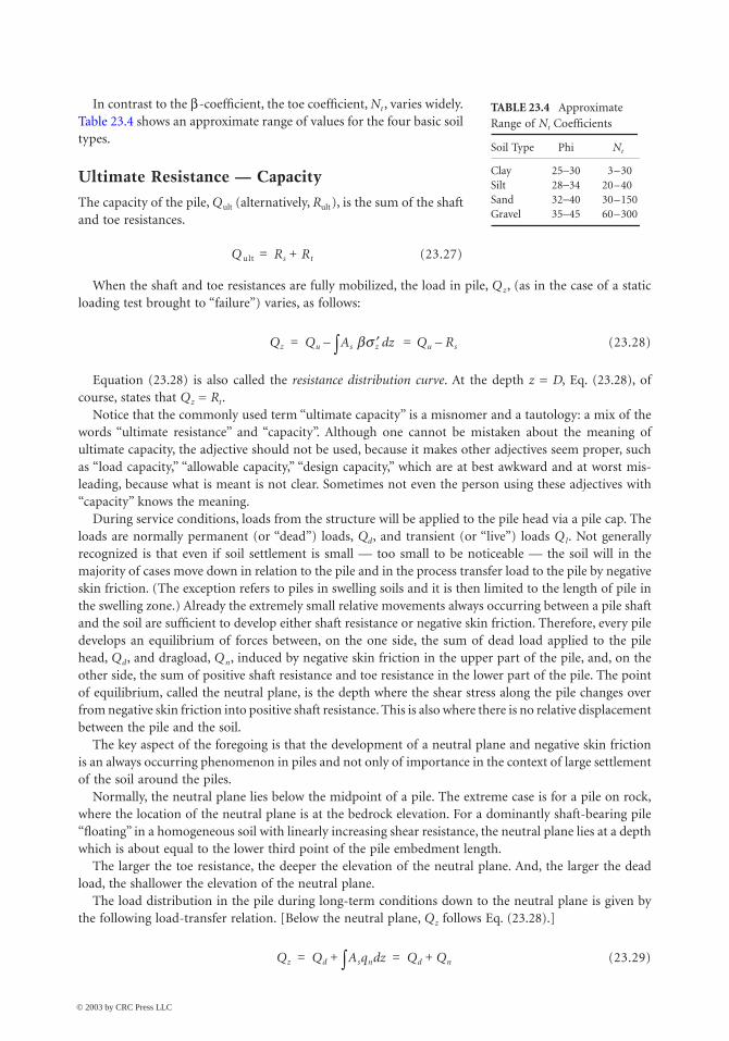
In contrast to the b-coefficient, the toe coefficient, Nt , varies widely.Table 23.4 shows an approximate range of values for the four basic soiltypes.

Ultimate Resistance — Capacity

The capacity of the pile, Qult (alternatively, Rult), is the sum of the shaftand toe resistances.

(23.27)

When the shaft and toe resistances are fully mobilized, the load in pile, Qz, (as in the case of a staticloading test brought to “failure”) varies, as follows:

(23.28)

Equation (23.28) is also called the resistance distribution curve. At the depth z = D, Eq. (23.28), ofcourse, states that Qz = Rt.

Notice that the commonly used term “ultimate capacity” is a misnomer and a tautology: a mix of thewords “ultimate resistance” and “capacity”. Although one cannot be mistaken about the meaning ofultimate capacity, the adjective should not be used, because it makes other adjectives seem proper, suchas “load capacity,” “allowable capacity,” “design capacity,” which are at best awkward and at worst mis-leading, because what is meant is not clear. Sometimes not even the person using these adjectives with“capacity” knows the meaning.

During service conditions, loads from the structure will be applied to the pile head via a pile cap. Theloads are normally permanent (or “dead”) loads, Qd, and transient (or “live”) loads Ql. Not generallyrecognized is that even if soil settlement is small — too small to be noticeable — the soil will in themajority of cases move down in relation to the pile and in the process transfer load to the pile by negativeskin friction. (The exception refers to piles in swelling soils and it is then limited to the length of pile inthe swelling zone.) Already the extremely small relative movements always occurring between a pile shaftand the soil are sufficient to develop either shaft resistance or negative skin friction. Therefore, every piledevelops an equilibrium of forces between, on the one side, the sum of dead load applied to the pilehead, Qd, and dragload, Qn, induced by negative skin friction in the upper part of the pile, and, on theother side, the sum of positive shaft resistance and toe resistance in the lower part of the pile. The pointof equilibrium, called the neutral plane, is the depth where the shear stress along the pile changes overfrom negative skin friction into positive shaft resistance. This is also where there is no relative displacementbetween the pile and the soil.

The key aspect of the foregoing is that the development of a neutral plane and negative skin frictionis an always occurring phenomenon in piles and not only of importance in the context of large settlementof the soil around the piles.

Normally, the neutral plane lies below the midpoint of a pile. The extreme case is for a pile on rock,where the location of the neutral plane is at the bedrock elevation. For a dominantly shaft-bearing pile“floating” in a homogeneous soil with linearly increasing shear resistance, the neutral plane lies at a depthwhich is about equal to the lower third point of the pile embedment length.

The larger the toe resistance, the deeper the elevation of the neutral plane. And, the larger the deadload, the shallower the elevation of the neutral plane.

The load distribution in the pile during long-term conditions down to the neutral plane is given bythe following load-transfer relation. [Below the neutral plane, Qz follows Eq. (23.28).]

(23.29)

TABLE 23.4 Approximate Range of Nt Coefficients

Soil Type Phi Nt

Clay 25-30 3–30Silt 28-34 20–40Sand 32-40 30–150Gravel 35-45 60–300

Q ult Rs Rt+=

Qz Qu As bs ¢z zdÚ– Qu Rs–= =

Qz Qd Asqn zdÚ+ Qd Qn+= =



The transition between the load-resistance curve [Eq. (23.27)] and the load-transfer curve [Eq. (23.28)]is in reality not the sudden kink the equations suggest, but a smooth transition over some length of pile,about 4 to 8 pile diameters above and below the neutral plane. (The length of this transition zone varieswith the type of soil at the neutral plane.) Thus, the theoretically calculated value of the maximum loadin the pile is higher than the real value. That is, it is easy to overestimate the magnitude of the dragload.

Critical Depth

Many texts suggest the existence of a so-called “critical depth” below which the shaft and toe resistanceswould be constant and independent of the increasing effective stress. This concept is a fallacy based onpast incorrect interpretation of test data and should not be applied.

Effect of Installation

Whether a pile is installed by driving or by other means, the installation affects, disturbs, the soil. It isdifficult to determine the magnitude of the shaft and toe resistances existing before the disturbance fromthe pile installation has subsided. For instance, presence of dissipating excess pore pressures causesuncertainity in the magnitude of the effective stress in the soil, ongoing strength gain due to reconsoli-dation is hard to estimate, etc. Such installation effects can take a long time to disappear, especially inclays. They can be estimated in an effective stress analysis using suitable assumptions as to the distributionof pore pressure along the pile at any particular time. Usually, to calculate the installation effect, a goodestimate can be obtained by imposing excess pore pressures in the fine-grained soil layers, taking carethat the pore pressure must not exceed the total overburden stress. By restoring the pore pressure valuesto the original conditions, which will prevail when the induced excess pore pressures have dissipated, thelong-term capacity is found.

Residual Load

The dissipation of induced excess pore pressures is called reconsolidation. Reconsolidation after installa-tion of a pile imposes load (residual load) in the pile by negative skin friction in the upper part of thepile, which is resisted by positive shaft resistance in the lower part of the pile and some toe resistance.The quantitative effect of including, as opposed to not to, the residual load in the analysis is that theshaft resistance becomes smaller and the toe resistance becomes larger. If the residual load is not recog-nized in the evaluation of results from a static loading test, totally erroneous conclusions will be drawnfrom the test: The shaft resistance appears larger than the true value, while the toe resistance appearscorrespondingly smaller, and if the resistance distribution is determined from a force gauge in the pile,zeroed at the start of the test, a “critical depth” will seem to exist. For more details on this effect and howto analyze the force gauge data to account for the residual load, see Altaee et al. [1992, 1993].

Analysis of Capacity for Tapered Piles

Many piles are not cylindrical or otherwise uniform in shape throughout the length. The most commonexample is the wood pile, which is conical in shape. Step-tapered piles are also common, consisting oftwo or more concrete-filled steel pipes of different diameters connected to each other, the larger abovethe smaller. Sometimes a pile can consist of a steel pipe with a conical section immediately above thepile toe, for example, the Monotube pile, which typically has a 25 feet (7.6 m) long conical end section,tapering the diameter down from 14 inches (355 mm) to 8 inches (203 mm). Piles can have an uppersolid concrete section and a bottom H-pile extension.

For the step-tapered piles, obviously each “step” provides an extra resistance point, which needs to beconsidered in an analysis. (The GRLWEAP wave equation program [GRL, 1993], for example, can modela pile with one diameter change as having a second pile toe at the location of the step). Similarly, in a staticanalysis, each such step can be considered as a donut-shaped extra pile toe and assigned a corresponding


Foundations 23-21

toe resistance per Eq. (23.26). Each such extra toe resistance value is then added to the shaft resistancecalculated using the actual pile diameter.

Piles with a continuous taper (conical piles) are less easy to analyze. Nordlund [1963] suggested ataper correction factor to use to increase the unit shaft resistance in sand for conical piles. The correctionfactor is a function of the taper angle and the soil friction angle. A taper angle of 1∞ (0.25 inch/foot) ina sand with a 35∞ friction angle would give a correction factor of about 4. At an angle of 0.5∞, the factorwould be about 2.

A more direct calculation method is to “step” the calculation in sub-layers of some thickness and atthe bottom of each such sub-layer project the donut-shaped diameter change, which then is treated asan extra toe similar to the analysis of the step-taper pile. The shaft resistance is calculated using the meandiameter of the pile over the same “stepped” length. The shaft resistance over each such particular lengthconsists of the sum of the shaft resistance and the extra-toe resistance. This method requires that a toecoefficient, Nt , be assigned to each soil layer.

The taper does not come into play for negative skin friction. This means that, when determining thedragload, the effect of the taper should be excluded. Below the neutral plane, however, the effect shouldbe included. Therefore, the taper will influence the location of the neutral plane (because the taperincreases the positive shaft resistance below the neutral plane).

Factor of Safety

In a pile design, one must distinguish between the design for bearing capacity and design for structuralstrength. The former is considered by applying a factor of safety to the pile capacity according toEq. (23.27). The capacity is determined considering positive shaft resistance developed along the fulllength of the pile plus full toe resistance. Notice that no allowance is given for the dragload. If design isbased on only theoretical analysis, the usual factor of safety is about 3.0. If based on the results of aloading test, static or dynamic, the factor of safety is reduced, depending on reliance on and confidencein the capacity value, and importance and sensitivity of the structure to foundation deformations. Factorsof safety as low as 1.8 have then been used in actual design, but usually the lower bound is 2.0.

Design for structural strength applies to a factor of safety applied to the loads acting at the pile headand at the neutral plane. At the pile head, the loads consist of dead and live load combined with bendingat the pile head, but no dragload. At the neutral plane, the loads consist of dead load and dragload, butno live load. Live load and dragload cannot occur at the same time and must, therefore, not be combinedin the analysis. It is recommended that for straight and undamaged piles the allowable maximum loadat the neutral plane be limited to 70% of the pile strength. For composite piles, such as concrete-filledpipe piles, the load should be limited to a value that induces a maximum compression strain of 1.0millistrain into the pile with no material becoming stressed beyond 70% of its strength. The calculationsare interactive inasmuch a change of the load applied to a pile will change the location of the neutralplane and the magnitude of the maximum load in the pile.

The third aspect in the design, calculation of settlement, pertains more to pile groups than to singlepiles. In extending the approach to a pile group, it must be recognized that a pile group is made up ofa number of individual piles which have different embedment lengths and which have mobilized the toeresistance to a different degree. The piles in the group have two things in common, however: They areconnected to the same stiff pile cap and, therefore, all pile heads move equally, and the piles must allhave developed a neutral plane at the same depth somewhere down in the soil (long-term condition, ofcourse).

Therefore, it is impossible to ensure that the neutral plane is common for the piles in the group, withthe mentioned variation of length, etc., unless the dead load applied to the pile head from the cap differsbetween the piles. This approach can be used to discuss the variation of load within a group of stifflyconnected piles. A pile with a longer embedment below the neutral plane or one having mobilized alarger toe resistance as opposed to other piles will carry a greater portion of the dead load on the group.On the other hand, a shorter pile, or one with a smaller toe resistance as opposed to other piles in the



group, will carry a smaller portion of the dead load. If a pile is damaged at the toe, it is possible that thepile exerts a negative — pulling — force at the cap and thus increases the total load on the pile cap.

An obvious result of the development of the neutral plane is that no portion of the dead load istransferred to the soil via the pile cap, unless, of course, the neutral plane lies right at the pile cap andthe entire pile group is failing.

Above the neutral plane, the soil moves down relative to the pile; below the neutral plane, the pilemoves down into the soil. Therefore, at the neutral plane, the relative movement between the pile andthe soil is zero, or, in other words, whatever the settlement of the soil that occurs at the neutral plane isequal to the settlement of the pile (the pile group) at the neutral plane. Between the pile head and theneutral plane, only deformation of the pile due to load occurs and this is usually minor. Therefore,settlement of the pile and the pile group is governed by the settlement of the soil at and below the neutralplane. The latter is influenced by the stress increase from the permanent load on the pile group and othercauses of load, such as the fill. A simple method of calculation is to exchange the pile group for anequivalent footing of area equal to the area of the pile cap placed at the depth of the neutral plane. Theload on the pile group load is then distributed as a stress on this footing calculating the settlement ofthis footing stress in combination with all other stress changes at the site, such as the earth fill, potentialgroundwater table changes, adjacent excavations, etc. Notice that the portion of the soil between theneutral plane and the pile toe depth is “reinforced” with the piles and, therefore, not very compressible.In most cases, the equivalent footing is best placed at the pile toe depth (or at the level of the average ofthe pile toe depths).

Empirical Methods for Determining Axial Pile Capacity

For many years, the N-index of standard penetration test has been used to calculate capacity of piles.Meyerhof [1976] compiled and rationalized some of the wealth of experience available and recommendedthat the capacity be a function of the N-index, as follows:

(23.30)

where m = a toe coefficientn = a shaft coefficientN = N-index at the pile toeN = average N-index along the pile shaftAt = pile toe areaAs = unit shaft area; circumferential areaD = embedment depth

For values inserted into Eq. (23.30) using base SI units — that is, R in newton, D in meter, and A inm2 — the toe and shaft coefficients, m and n, become:

m = 400 · 103 for driven piles and 120 · 103 for bored piles (N/m2)n = 2 · 103 for driven piles and 1 · 103 for bored piles (N/m3)

For values inserted into Eq. (23.30) using English units with R in ton, D in feet, and A in ft2, the toeand shaft coefficients, m and n, become:

m = 4 for driven piles and 1.2 for bored piles (N/m2)n = 0.02 for driven piles and 0.01 for bored piles (N/m3)

The standard penetration test (SPT) is a subjective and highly variable test. The test and the N-indexhave substantial qualitative value, but should be used only very cautiously for quantitative analysis. TheCanadian Foundation Engineering Manual [Canadian Geotechnical Society, 1985] includes a listing of

R Rt Rs+ mNAt nNAsD+= =


Foundations 23-23

the numerous irrational factors influencing the N-index. However, when the use of the N-index isconsidered with the sample of the soil obtained and related to a site- and area-specific experience, thecrude and decried SPT test does not come out worse than other methods of analyses.

The static cone penetrometer resembles a pile. There is shaft resistance in the form of so-called localfriction measured immediately above the cone point, and there is toe resistance in the form of the directlyapplied and measured cone-point pressure.

When applying cone penetrometer data to a pile analysis, both the local friction and the point pressuremay be used as direct measures of shaft and toe resistances, respectively. However, both values can showa considerable scatter. Furthermore, the cone-point resistance, (the cone-point being small compared toa pile toe) may be misleadingly high in gravel and layered soils. Schmertmann [1978] has indicated anaveraging procedure to be used for offsetting scatter, whether caused by natural (real) variation in thesoil or inherent in the test.

The piezocone, which is a cone penetrometer equipped with pore pressure measurement devices atthe point, is a considerable advancement on the static cone. By means of the piezocone, the coneinformation can be related more dependably to soil parameters and a more detailed analysis can beperformed. Soil is variable, however, and the increased and more representative information obtainedalso means that a certain digestive judgment can and must be exercised to filter the data for computationof pile capacity. In other words, the designer is back to square one: more thoroughly informed and lessliable to jump to false conclusions, but certainly not independent of site-specific experience. Eslami andFellenius (1997) and Fellenius and Eslami (2000) have presented comprehensive information on soilprofiling and analysis on pile capacity based on CPT data.

The Lambda MethodVijayvergiya and Focht [1972] compiled a large number of results from static loading tests on essentiallyshaft-bearing piles in reasonably uniform soil and found that, for these test results, the mean unit shaftresistance is a function of depth and can be correlated to the sum of the mean overburden effective stressplus twice the mean undrained shear strength within the embedment depth, as follows.

(23.31)

where rm = mean shaft resistance along the pilel = the lambda correlation coefficient

sm = mean overburden effective stresscm = mean undrained shear strength

The correlation factor is called “lambda” and it is a function of pile embedment depth, reducing withincreasing depth, as shown in Table 23.5.

The lambda method is almost exclusively applied to determining the shaft resistance for heavily loadedpipe piles for offshore structures in relatively uniform soils.

TABLE 23.5 Approximate Values of l

Embedment l(ft) (m) (-)

0 0 0.5010 3 0.3625 7 0.2750 15 0.2275 23 0.17

100 30 0.15200 60 0.12

rs l s ¢m 2cm+( )=



Field Testing for Determining Axial Pile Capacity

The capacity of a pile is of most reliable value when determined in a full-scale field test. However, despitethe numerous static loading tests that have been carried out and the many papers that have reported onsuch tests and their analyses, the understanding of static pile testing in current engineering practice leavesmuch to be desired. The reason is that engineers have concerned themselves with mainly one question —“Does the pile have a certain least capacity?” — finding little of practical value in analyzing the pile–soilinteraction, the load transfer.

A static loading test is performed by loading a pile with a gradually or stepwise increasing force whilemonitoring the movement of the pile head. The force is obtained by means of a hydraulic jack reactingagainst a loaded platform or anchors.

The American Society for Testing and Materials, ASTM, publishes three standards, D-1143, D-3689,and D-3966, for static testing of a single pile in axial compression, axial uplift, and lateral loading,respectively. The ASTM standards detail how to arrange and perform the pile test. Wisely, they do notinclude how to interpret the tests, because this is the responsibility of the engineer in charge, who is theonly one with all the site-and project-specific information necessary for the interpretation.

The most common test procedure is the slow maintained load method referred to as the “standardloading procedure” in the ASTM Designation D-1143 and D-3689, in which the pile is loaded in eightequal increments up to a maximum load, usually twice a predetermined allowable load. Each load levelis maintained until zero movement is reached, defined as 0.25 mm/hr (0.01 in./hr). The final load, the200 percent load, is maintained for a duration of 24 hours. The “standard method” is very time-consuming, requiring from 30 to 70 hours to complete. It should be realized that the words “zeromovement” are very misleading: The “zero” movement rate mentioned is equal to a movement of morethan 2 m (7 ft) per year!

Each of the eight load increments is placed onto the pile very rapidly; as fast as the pump can raisethe load, which usually takes about 20 seconds to 2 minutes. The size of the load increment in the“standard procedure” — 12.5 percent of the maximum load — means that each such increase of load isa shock to the pile and the soil. Smaller increments that are placed more frequently disturb the pile less,and the average increase of load on the pile during the test is about the same. Such loading methodsprovide more consistent, reliable, and representative data for analysis.

Tests that consist of load increments applied at constant time intervals of 5, 10, or 15 minutes arecalled quick maintained-load tests or just “quick tests.” In a quick test, the maximum load is not normallykept on the pile longer than any other load before the pile is unloaded. Unloading is done in about tensteps of no longer duration than a few minutes per load level. The quick test allows for applying one ormore load increments beyond the minimum number that the particular test is designed for, that is,making use of the margin built into the test. In short, the quick test is, from the technical, practical, andeconomic points of view, superior to the “standard loading procedure.”

A quick test should aim for 25 to 40 increments with the maximum load determined by the amountof reaction load available or the capacity of the pile. For routine cases, it may be preferable to stay at amaximum load of 200 percent of the intended allowable load. For ordinary test arrangements, whereonly the load and the pile head movement are monitored, time intervals of 10 minutes are suitable andallow for the taking of 2 to 4 readings for each increment. When testing instrumented piles, where theinstruments take a while to read (scan), the time interval may have to be increased. To go beyond20 minutes, however, should not be necessary. Nor is it advisable, because of the potential risk forinfluence of time-dependent movements, which may impair the test results. Usually, a quick test iscompleted within three to six hours.

In routine tests, cyclic loading or even single unloading and loading phases must be avoided, as theydo little more than destroy the possibility of a meaningful analysis of the test results. There is absolutelyno logic in believing that anything of value on load distribution and toe resistance can be obtained froman occasional unloading or from one or a few “resting periods” at certain load levels, when consideringthat we are testing a unit that is subjected to the influence of several soil types, is subjected to residual


Foundations 23-25

stress of unknown magnitude, exhibits progressive failure, etc., and when all we know is what is appliedand measured at the pile head.

Interpretation of Failure Load

For a pile that is stronger than the soil, the failure load is reached when rapid movement occurs undersustained or slightly increased load (the pile plunges). However, this definition is inadequate, becauseplunging requires large movements. To be useful, a definition of failure load must be based on somemathematical rule and generate a repeatable value that is independent of scale relations and the opinionsof the individual interpreter. Furthermore, it has to consider the shape of the load-movement curve or,if not, it must consider the length of the pile (which the shape of the curve indirectly does).

Fellenius [1975, 1980] compiled several methods used for interpreting failure or limit loads from aload-movement curve of a static loading test. The most well-known method is the offset limit methodproposed by Davisson [1972]. This limit load is defined as the load corresponding to the movement thatexceeds the elastic compression of the pile by an offset of 4 mm (0.15 inch) plus a value equal to thediameter of the pile divided by 120. It must be realized, however, that the offset limit load is a deformationlimit that is determined taking into account the stiffness and length of the pile. It is not necessarily equalto the failure load of the pile.

The offset limit has the merit of allowing the engineer, when proof testing a pile for a certain allowableload, to determine in advance the maximum allowable movement for this load with consideration of thelength and size of the pile. Thus, contract specifications can be drawn up including an acceptance criterionfor piles proof tested according to quick-testing methods. The specifications can simply call for a test toat least twice the design load, as usual, and declare that at a test load equal to a factor F times the designload the movement shall be smaller than the Davisson offset from the elastic column compression of thepile. Normally, F would be chosen within a range of 1.8 to 2.0. The acceptance criterion could besupplemented with the requirement that the safety factor should also be smaller than a certain minimumvalue calculated on pile bearing failure defined according to the 80% criterion or other preferred criterion.

Influence of Errors

A static loading test is usually considered a reliable method for determining the capacity of a pile. However,even when using new manometers and jacks and calibrating them together, the applied loads is usuallysubstantially overestimated. The error is usually about 10% to 15% of the applied load. Errors as largeas 30% to 40% are not uncommon.

The reason for the error is that the jacking system is required to both provide the load and to measureit, and because load cells with moving parts are considerably less accurate than those without moving parts.For example, when calibrating testing equipment in the laboratory, one ensures that no eccentric loading,bending moments, or temperature variations influence the calibration. In contrast, all of these adversefactors are at hand in the field and influence the test results to an unknown extent, unless a load cell is used.

The above deals with the error of the applied load. The error in movement measurement can also becritical. Such errors do not originate in the precision of the reading — the usual precision is more thanadequate — but in undesirable influences, such as heave or settlement of the reference beam duringunloading the ground when loading the pile. For instance, one of the greatest spoilers of a loading testis the sun: The reference beam must be shielded from sunshine at all times.

Dynamic Analysis and Testing

The penetration resistance of driven piles provides a direct means of determining bearing capacity of apile. In impacting a pile, a short-duration force wave is induced in the pile, giving the pile a downwardvelocity and resulting in a small penetration of the pile. Obviously, the larger the number of blowsnecessary to achieve a certain penetration, the stronger the soil. Using this basic principle, a large numberof so-called pile-driving formulas have been developed for determining pile-bearing capacity. All these



formulas are based on equalizing potential energy available for driving in terms of weight of hammertimes its height of fall (stroke) with the capacity times penetration (“set”) for the blow. The penetrationvalue often includes a loss term.

The principle of the dynamic formulas is fundamentally wrong as wave action is neglected along witha number of other aspects influencing the penetration resistance of the pile. Nevertheless, pile-drivingformulas have been used for many years and with some degree of success. However, success has beendue less to the theoretical correctness of the particular formulas used and more to the fact that the userspossessed adequate practical experience to go by. When applied to single-acting hammers, use of adynamic formula may have some justification. However, dynamic formulas are the epitome of an out-moded level of technology and they have been or must be replaced by modern methods, such as thewave equation analysis and dynamic measurements, which are described below.

Pile-driving formulas or any other formula applied to vibratory hammers are based on a misconcep-tion. Vibratory driving works by eliminating resistance to penetration, not by overcoming it. Therefore,records of penetration combined with frequency, energy, amplitudes, and so on can relate only to theresistance not eliminated, not to the static pile capacity after the end of driving.

Pile-driving hammers are rated by the maximum potential energy determined as the ram weight timesthe maximum ram travel. However, diesel hammers and double-acting air/steam hammers, but alsosingle-acting air/steam hammers, develop their maximum potential energy only during favorable com-binations with the pile and the soil. Then, again, the energy actually transferred to the pile may vary dueto variation in cushion properties, pile length, toe conditions, etc. Therefore, a relation between thehammer rated energy and measured transferred energy provides only very little information on thehammer.

For reliable analysis, all aspects influencing the pile driving and penetration resistance must be con-sidered: hammer mass and travel, combustion in a diesel hammer, helmet mass, cushion stiffness, hammerefficiency, soil strength, viscous behavior of the soil, and elastic properties of the pile, to mention some.This analysis is made by means of commercially available wave equation programs, such as the GRLWEAP[GRL, 1993].

However, the parameters used as input into a wave equation program are really variables with certainranges of values and the number of parameters included in the analysis is large. Therefore, the result ofan analysis is only qualitatively correct, and not necessarily quantitatively correct, unless it is correlatedto observations. The full power of the wave equation analysis is only realized when combined withdynamic measurements during pile driving by means of transducers attached to the pile head. The impactby the pile-driving hammer produces strain and acceleration in the pile which are picked up by thetransducers and transmitted via a cable to a data acquisition unit (the Pile Driving Analyzer), which isplaced in a nearby monitoring station. The complete generic field-testing procedure is described in theAmerican Society for Testing and Materials, Standard for Dynamic Measurements, ASTM D-4945.

Dynamic testing, also called dynamic monitoring, is performed with the Pile Driving Analyzer (PDA).The PDA measurements provide much more information than just the value of the capacity of the pile,such as the energy transferred into the pile, the stresses in the pile, and the hammer performance. Thedynamic data can be subjected to special analyses and provide invaluable information for determiningthat the piles are installed correctly, that the soil response is what was assumed in the design, and muchmore. For details, see Rausche et al. [1985] and Hannigan [1990]. Should difficulties develop with thepile driving at the site, the dynamic measurements can normally determine the reason for the difficultiesand how to eliminate them. In the process, the frequent occurrence of having difficulties grow into adispute between the contractor, the engineer, and the owner is avoided.

The dynamic measurements provide quantitative information of how the pile hammer functions, thecompression and tension stresses that are imposed on the pile during the driving, and how the soilresponds to the driving of the pile, including information pile static capacity. The dynamic measurementscan also be used to investigate damage and defects in the pile, such as voids, cracks, spalling, local buckling,etc.


Foundations 23-27

Dynamic records are routinely subjected to a detailed analysis called the CAPWAP signal matchinganalysis [Rausche et al., 1972]. The CAPWAP analysis provides, first of all, a calculated static capacityand the distribution of resistance along the pile. However, it also provides several additional data, forexample, the movement necessary to mobilize the full shear resistance in the soil (the quake) and dampingvalues for input in a wave equation analysis.

Pile Group Example: Axial Design

The design approach is illustrated in the following example: A group of 25 piles consisting of 355-mmdiameter, closed-end steel pipes are to be driven at equal spacing and in a square configuration at a sitewith the soil profile equal to that described earlier as background to Table 23.1. The 1.5-m earth fill over36 m2 area will be placed symmetrically around the pile group. The pile cap is 9.0 m2 and placed levelwith the ground surface.

Each pile will be subjected to dead and live loads of 800 kN and 200 kN, respectively. The soilsinvestigation has established a range of values of the soil parameters necessary for the calculations, suchas density, compressibility, consolidation coefficient, as well as the parameters ( b and Nt) used in theeffective stress calculations of load transfer. A load-transfer analysis is best performed using a range(boundary values) of b and Nt parameters, which differentiate upper and lower limits of reasonablevalues. The analysis must include several steps in approximately the following order.

Determine first the range of installation length (using the range of effective stress parameters) as basedon the required at-least capacity, which is stated, say, to be at least equal to the sum of the loads timesa factor of safety of 3.0: 3.0(800 + 200) = 3000 kN.

To obtain a capacity of 3000 kN, applying the lower boundary of b and Nt, the piles have to be installedto a penetration into the sandy till layer of 5 m, that is, to a depth of 32 m. Table 23.6 presents the resultsof the load-transfer calculations for this embedment depth. The calculations have been made with theUnipile program [Goudreault and Fellenius, 1990] and the results are presented in the format of a handcalculation to ease verifying the computer calculations. The precision indicated by stress values givenwith two decimals is to assist in the verification of the calculations and does not suggest a correspondinglevel of accuracy. Moreover, the effect of the 9 m2 “hole” in the fill for the pile cap was ignored in thecalculation. Were its effect to be included in the calculations, the calculated capacity would reduce by93 kN or the required embedment length increase by 0.35 m.

The calculated values have been plotted in Fig. 23.5 in the form of two curves: a resistance curve givingthe load transfer as in a static loading test to failure (3000 kN); and a load curve for long-term conditions,starting at the dead load of 800 kN and increasing due to negative skin friction to a maximum at theneutral plane. The load and resistance distributions for the example pile follow Eqs. (23.27) and (23.28).

Pile Group Settlement

The piles have reached well into the sand layers, which will not compress much for the increase of effectivestress. Therefore, settlement of the pile group will be minimal and will not govern the design.

Installation Phase

The calculations shown above pertain to the service condition of the pile and are not quite representativefor the installation (construction) phase. First, when installing the piles (these piles will be driven), theearth fill is not yet placed, which means that the effective stress in the soil is smaller than during theservice conditions. More important, during the pile driving, large excess pore pressures are induced inthe soft clay layer and, probably, also in the silty sand, which further reduces the effective stress. Ananalysis imposing increased pore pressures in these layers suggests that the capacity is about 2200 kN atthe end of the initial driving (EOID) using the depth and effective stress parameters indicated in Table 23.6for the 32 m installation depth. The subsequent dissipation of the pore pressures will result in an about600-kN soil increase of capacity due to set-up. (The stress increase due to the earth fill will provide theadditional about 200 kN to reach the 3000-kN service capacity.)



The design must include the selection of the pile-driving hammer, which requires the use of softwarefor wave equation analysis, called WEAP analysis [Goble et al., 1980; GRL, 1993; Hannigan, 1990]. Thisanalysis requires input of soil resistance in the form as result of static load-transfer analysis. For theinstallation (initial driving) conditions, the input is calculated considering the induced pore pressures.For restriking conditions, the analysis should consider the effect of soil set-up.

By means of wave equation analysis, pile capacity at initial driving — in particular the EOID — andrestriking (RSTR) can be estimated. However, the analysis also provides information on what driving

TABLE 23.6 Calculation of Pile Capacity

Area As = 1.115 m2/mArea At = 0.009 m2

Factor of Safety = 3.2

Live Load, Ql = 200 kNDead Load, Qd = 800 kNTotal Load = 1000 kNDepth to Neutral Plane = 26.51 m

Shaft Resistance, Rs = 1817 kNToe Resistance, Rt = 1205 kNTotal Resistance, Ru = 3021 kNLoad at Neutral Plane = 1911 kN

Depth(m)

TotalStress(kPa)

PorePres.(kPa)

Eff.Stress(kPa)

Incr.Rs

(kN)Qd + Qn

(kN)QU – Rs

(kN)

Layer 1 Sandy Silt r = 2000 kg/m3 b = 0.40

0.00 30.00 0.00 30.00 0.0 800 32321.00 (GWT) 48.40 0.00 48.40 17.5 817 32154.00 104.30 30.00 74.30 82.1 900 3133

Layer 2 Soft Clay r = 1700 kg/m3 b = 0.30

4.00 104.30 30.00 74.30 900 31335.00 120.13 43.53 76.60 25.2 925 31086.00 136.04 57.06 78.98 26.0 951 30827.00 152.03 70.59 81.44 26.8 978 30558.00 168.08 84.12 83.96 27.7 1005 30279.00 184.20 97.65 86.55 28.5 1034 2999

10.00 200.37 111.18 89.20 29.4 1063 296911.00 216.60 124.71 91.89 30.3 1094 293912.00 232.88 138.24 94.64 31.2 1125 290813.00 249.19 151.76 97.43 32.1 1157 287614.00 265.55 165.29 100.26 33.1 1190 284215.00 281.95 178.82 103.12 34.0 1224 280816.00 298.38 192.35 106.03 35.0 1259 277317.00 314.84 205.88 108.96 36.0 1295 273718.00 331.33 219.41 111.92 37.0 1332 270119.00 347.85 232.94 114.91 37.9 1370 266320.00 364.40 246.47 117.93 39.0 1409 262421.00 380.97 260.00 120.97 40.0 1449 2584

Layer 3 Silty Sand r = 2100 kg/m3 b = 0.50

21.00 380.97 260.00 120.97 1449 258422.00 401.56 270.00 131.56 70.4 1519 251323.00 422.17 280.00 142.17 76.3 1596 243724.00 442.80 290.00 152.80 82.2 1678 235525.00 463.45 300.00 163.45 88.2 1766 226726.00 484.11 310.00 174.11 94.1 1860 217227.00 504.80 320.00 184.80 100.1 1960 2072

Layer 4 Ablation Till r = 2100 kg/m3 b = 0.50

27.00 504.80 320.00 184.80 1960 207230.00 569.93 350.00 219.93 372.4 2332 170032.00 613.41 370.00 243.41 285.1 2617 1205

N t = 50

Note: Calculations by means of UNIPILE.


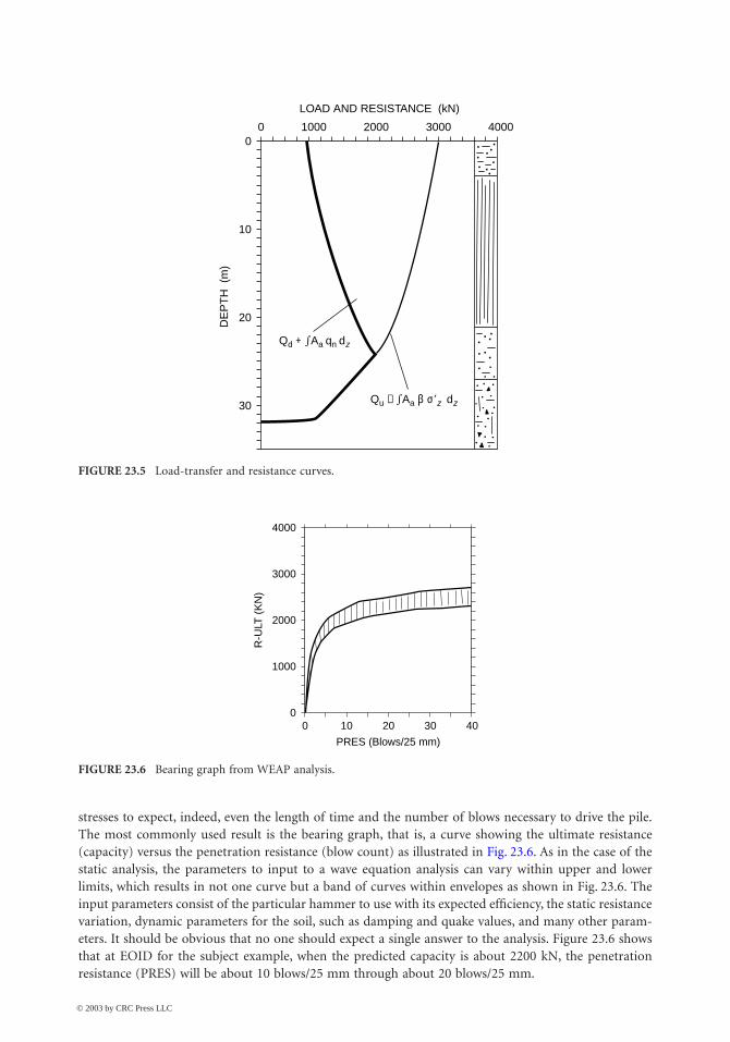
Foundations 23-29

stresses to expect, indeed, even the length of time and the number of blows necessary to drive the pile.The most commonly used result is the bearing graph, that is, a curve showing the ultimate resistance(capacity) versus the penetration resistance (blow count) as illustrated in Fig. 23.6. As in the case of thestatic analysis, the parameters to input to a wave equation analysis can vary within upper and lowerlimits, which results in not one curve but a band of curves within envelopes as shown in Fig. 23.6. Theinput parameters consist of the particular hammer to use with its expected efficiency, the static resistancevariation, dynamic parameters for the soil, such as damping and quake values, and many other param-eters. It should be obvious that no one should expect a single answer to the analysis. Figure 23.6 showsthat at EOID for the subject example, when the predicted capacity is about 2200 kN, the penetrationresistance (PRES) will be about 10 blows/25 mm through about 20 blows/25 mm.

FIGURE 23.5 Load-transfer and resistance curves.

FIGURE 23.6 Bearing graph from WEAP analysis.

Qu − �Aa β σ′z dz

Qd + �Aa qn dz

0 1000 2000 3000 40000

10

20DE

PT

H (

m)

LOAD AND RESISTANCE (kN)

30

4000

3000

2000

1000

00 10 20

PRES (Blows/25 mm)

R-U

LT (

KN

)

30 40



Notice that the wave equation analysis postulates observation of the actual penetration resistance whendriving the piles, as well as a preceding static analysis. Then, common practice is to combine the analyseswith a factor of safety ranging from 2.5 through 3.0.

Figure 23.6 demonstrates that the hammer selected for the driving cannot drive the pile against the3000-kN capacity expected after full set-up. That is, restriking cannot prove out the capacity. This is acommon occurrence. Bringing in a larger hammer may be a costly proposition. It may also be quiteunnecessary. If the soil profile is well known, the static analysis correlated to the soil profile and to carefulobservation during the entire installation driving for a few piles, sufficient information is usually obtainedto support a satisfactory analysis of the pile capacity and load transfer. That is, the capacity after set-upis inferred and sufficient for the required factor of safety.

When conditions are less consistent, when savings may result, and when safety otherwise suggests itto be good practice, the pile capacity is tested directly. Conventionally, this is accomplished by means ofa static loading test. Since about 1975, dynamic tests have likewise often been performed. Static tests arecostly and time-consuming, and are therefore usually limited to one or a few piles. In contrast, dynamictests can be obtained quickly and economically and can be performed on several piles, thus providingassurance in numbers. For larger projects, static and dynamic tests are often combined. More recently,a new testing method called Statnamic has been proposed [Bermingham and Janes, 1989]. The Statnamicmethod is particularly intended for high-capacity bored piles (drilled piers). The Osterberg O-Cell(Fellenius, 2001) is a very useful new tool for the geotechnical engineer to use when reliable separationof shaft and toe resistances is required. The O-cell is suitable for testing of both bored and drive piles.

When the capacity is determined by direct testing, the factor of safety of the design is reduced. Theusual range is from 2.0 to 2.2. When the design and the installation are tested by means of static or dynamicproof testing on the site, the factor of safety is often reduced to the range of 1.8 through 2.0. Notice thatresults of the tests must not just be given in terms of a capacity value (which can vary depending on howthe ultimate resistance is defined); the load transfer should also be included in the analysis.

All analyses for a project must apply the same factor of safety. Therefore, for the subject example,when the designer knows that the capacity will be verified by means of a direct test, the minimum factorof safety to apply reduces to about 2.2, say. That is, the piles need only be driven to a final (after set-up)capacity of 2000 kN or 2200 kN. Considering the initial driving conditions, the capacity at EOID couldbe limited to about 1600 kN and this should be obtainable at a penetration into the till of slightly lessthan one meter and a penetration resistance of 4 to 5 blow/25 mm. Then, the subsequent increase dueto set-up to 2200 kN is verified in a dynamic of static test combined with restriking to verify that thePRES values have increased to beyond about 10 blows/25 mm.

Summary of Axial Design of Piles

In summary, pile design consists of the following steps.

1. Compile soil data and perform a static analysis of the load transfer.2. Verify that the ultimate pile resistance (capacity) is at least equal to the factor of safety times the

sum of the dead and the live load (do not include the dragload in this calculation).3. Verify that the maximum load in the pile, which is the sum of the dead load and the dragload is

smaller than the structural strength of the pile divided by the appropriate factor of safety (usually1.5) times. (Do not include the live load in this calculation.)

4. Verify that the pile group settlement does not exceed the maximum deformation permitted by thestructural design.

5. Perform wave equation analysis to select the pile-driving hammer and to decide on the drivingand termination criteria (for driven piles).

6. Observe carefully the pile driving (construction) and verify that the work proceeds as anticipated.Document the observations (that is, keep a complete and carefully prepared log!).

7. When the factor of safety needs to be 2.5 or smaller, verify pile capacity by means of static ordynamic testing.


Foundations 23-31

Design of Piles for Horizontal Loading

Because foundation loads act in many different directions depending on the load combination, piles arerarely loaded in true axial direction only. Therefore, a more or less significant lateral component of thetotal pile load always acts in combination with an axial load. The imposed lateral component is resistedby the bending stiffness of the pile and the shear resistance mobilized in the soil surrounding the pile.

An imposed horizontal load can also be carried by means of inclined piles, if the horizontal componentof the axial pile load is at least equal to and acting in the opposite direction to the imposed horizontalload. Obviously, this approach has its limits, as the inclination cannot be impractically large. It should,preferably, not be greater than 4 (vertical) to 1 (horizontal). Also, only one load combination can providethe optimal lateral resistance.

In general, it is not correct to resist lateral loads by means of combining the soil resistance for thepiles (inclined as well as vertical) with the lateral component of the vertical load for the inclined piles.The reason is that resisting an imposed lateral load by means of soil shear requires the pile to moveagainst the soil. The pile will rotate due to such movement and an inclined pile will then either push upagainst or pull down from the pile cap, which will substantially change the axial load in the pile.

In design of vertical piles installed in a homogeneous soil and subjected to horizontal loads, anapproximate and usually conservative approach is to assume that each pile can sustain a horizontal loadequal to the passive earth pressure acting on an equivalent wall with depth of 6b and width 3b, where bis the pile diameter or face-to-face distance [Canadian Geotechnical Society, 1985].

Similarly, the lateral resistance of a pile group may be approximated by the soil resistance on the groupcalculated as the passive earth pressure over an equivalent wall with depth equal to 6b and width equal to:

(23.32)

where Le = equivalent widthL = the length, center-to-center, of the pile group in plan perpendicular to the direction of

the imposed loadsb = the width of the equivalent area of the group in plan parallel to the direction of the

imposed loads

The lateral resistance calculated according to Eq. (23.32) must not exceed the sum of the lateralresistance of the individual piles in the group. That is, for a group of n piles, the equivalent width of thegroup, Le, must be smaller than n times the equivalent width of the individual pile, 6b. For an imposedload not parallel to a side of the group, calculate for two cases, applying the components of the imposedload that are parallel to the sides.

The very simplified approach expressed above does not give any indication of movement. Nor does itdifferentiate between piles with fixed heads and those with heads free to rotate; that is, no considerationis given to the influence of pile bending stiffness. Because the governing design aspect with regard tolateral behavior of piles is lateral displacement, and the lateral capacity or ultimate resistance is ofsecondary importance, the usefulness of the simplified approach is very limited in engineering practice.

The analysis of lateral behavior of piles must involve two aspects:

1. Pile response. The bending stiffness of the pile, how the head is connected (free head, or fully orpartially fixed head).

2. Soil response. The input in the analysis must include the soil resistance as a function of themagnitude of lateral movement.

The first aspect is modeled by treating the pile as a beam on an “elastic” foundation, which isaccomplished by solving a fourth-degree differential equation with input of axial load on the pile, materialproperties of the pile, and the soil resistance as a nonlinear function of the pile displacement.

The derivation of lateral stress may make use of a simple concept called coefficient of subgrade reactionhaving the dimension of force per volume [Terzaghi, 1955]. The coefficient is a function of the soil density

Le L 2b+=



or strength, the depth below the ground surface, and the diameter (side) of the pile. In cohesionless soils,the following relation is used:

(23.33)

where ks = coefficient of horizontal subgrade reactionnh = coefficient related to soil densityz = depthb = pile diameter

The intensity of the lateral stress, pz, mobilized on the pile at depth z is then as follows:

(23.34)

where yz = the horizontal displacement of the pile at depth z. Combining Eqs. (23.33) and (23.34), we get

(23.35)

The relation governing the behavior of a laterally loaded pile is then as follows:

(23.36)

where Qh = lateral load on the pileEI = bending stiffness (flexural rigidity)Qv = axial load on the pile

Design charts have been developed that, for an input of imposed load, basic pile data, and soilcoefficients, provide values of displacement and bending moment. See, for instance, the CanadianFoundation Engineering Manual [Canadian Geotechnical Society, 1985].

The design charts cannot consider all the many variations possible in an actual case. For instance, thep – y curve can be a smooth rising curve, can have an ideal elastic-plastic shape, or can be decaying aftera peak value. As an analysis without simplifying shortcuts is very tedious and time-consuming, resort tocharts has been necessary in the past. However, with the advent of the personal computer, special softwarehas been developed, which makes the calculations easy and fast. In fact, as in the case of pile-drivinganalysis and wave equation programs, engineering design today has no need for computational simpli-fications. Exact solutions can be obtained as easily as approximate ones. Several proprietary and publicdomain programs are available for analysis of laterally loaded piles.

One must not be led to believe that, because an analysis is theoretically correct, the results also predictthe true behavior of the pile or pile group. The results must be correlated to pertinent experience and,lacking this, to a full-scale test at the site. If the experience is limited and funds are lacking for a full-scale correlation test, then a prudent choice is necessary of input data, as well as of margins and factorsof safety.

Designing and analyzing a lateral test is much more complex than for the case of axial behavior ofpiles. In service, a laterally loaded pile almost always has a fixed-head condition. However, a fixed-headtest is more difficult and costly to perform as opposed to a free-head test. A lateral test without inclusionof measurement of lateral deflection down the pile (bending) is of limited value. While an axial testshould not include unloading cycles, a lateral test should be a cyclic test and include a large number ofcycles at different load levels. The laterally tested pile is much more sensitive to the influence of neigh-boring piles than is the axially tested pile. Finally, the analysis of the test results is very complex andrequires the use of a computer and appropriate software.

ks nhzb--=

pz ksyzb=

pz nhyzz.=

Qh EI d 4y

dx4-------- Qv

d 2y

dx2-------- p–+=


Foundations 23-33

Seismic Design of Lateral Pile Behavior

Seismic design of lateral pile behavior is often taken as being the same as the conventional lateral design.A common approach is to assume that the induced lateral force to be resisted by piles is static and equalto a proportion, usually 10% of the vertical force acting on the foundation. If all the horizontal force isdesigned to be resisted by inclined piles, and all piles — including the vertical ones — are designed toresist significant bending at the pile cap, this approach is normally safe, albeit costly.

The seismic wave appears to the pile foundation as a soil movement forcing the piles to move withthe soil. The movement is resisted by the pile cap; bending and shear are induced in the piles; and ahorizontal force develops in the foundation, starting it to move in the direction of the wave. A half periodlater, the soil swings back, but the foundation is still moving in the first direction, and therefore theforces increase. This situation is not the same as the one originated by a static force.

Seismic lateral pile design consists of determining the probable amplitude and frequency of the seismicwave as well as the natural frequency of the foundation and structure supported by the piles. The firstrequirement is, as in all seismic design, that the natural frequency must not be the same as that of theseismic wave. Then the probable maximum displacement, bending, and shear induced at the pile cap areestimated. Finally the pile connection and the pile cap are designed to resist the induced forces.

There is at present a rapid development of computer software for use in detailed seismic design.

Defining Terms

Capacity — The maximum or ultimate soil resistance mobilized by a foundation unit.Capacity, bearing — The maximum or ultimate soil resistance mobilized by a foundation unit subjected

to downward loading.Dragload — The load transferred to a deep foundation unit from negative skin friction.Factor of safety — The ratio of maximum available resistance or of the capacity to the allowable stress

or load.Foundation — A system or arrangement of structural members through which the loads are transferred

to supporting soil or rock.Groundwater table — The upper surface of the zone of saturation in the ground.Load, allowable — The maximum load that may be safely applied to a foundation unit under expected

loading and soil conditions and determined as the capacity divided by the factor of safety.Neutral plane — The location where equilibrium exists between the sum of downward acting perma-

nent load applied to the pile and dragload due to negative skin friction and the sum of upwardacting positive shaft resistance and mobilized toe resistance. The neutral plane is also where therelative movement between the pile and the soil is zero.

Pile — A slender deep foundation unit, made of wood, steel, concrete, or combinations thereof, whichis either premanufactured and placed by driving, jacking, jetting, or screwing, or cast in situ ina hole formed by driving, excavating, or boring. A pile can be a non-displacement, low-displacement, or displacement type.

Pile head — The uppermost end of a pile.Pile point — A special type of pile shoe.Pile shaft — The portion of the pile between the pile head and the pile toe.Pile shoe — A separate reinforcement attached to the pile toe of a pile to facilitate driving, to protect

the lower end of the pile, and/or to improve the toe resistance of the pile.Pile toe — The lowermost end of a pile. (Use of terms such as pile tip, pile point, or pile end in the

same sense as pile toe is discouraged).Pore pressure — Pressure in the water and gas present in the voids between the soil grains minus the

atmospheric pressure.Pore pressure, artesian — Pore pressure in a confined body of water having a level of hydrostatic

pressure higher than the level of the ground surface.



Pore pressure, hydrostatic — Pore pressure varying directly with a free-standing column of water.Pore pressure elevation, phreatic — The elevation of a groundwater table corresponding to a hydro-

static pore pressure equal to the actual pore pressure.Pressure — Omnidirectional force per unit area. (Compare stress.)Settlement — The downward movement of a foundation unit or soil layer due to rapidly or slowly

occurring compression of the soils located below the foundation unit or soil layer, when thecompression is caused by an increase of effective stress.

Shaft resistance, negative — Soil resistance acting downward along the pile shaft because of an applieduplift load.

Shaft resistance, positive — Soil resistance acting upward along the pile shaft because of an appliedcompressive load.

Skin friction, negative — Soil resistance acting downward along the pile shaft as a result of downdragand inducing compression in the pile.

Skin friction, positive — Soil resistance acting upward along the pile shaft caused by swelling of thesoil and inducing tension in the pile.

Stress — Unidirectional force per unit area. (Compare pressure.)Stress, effective — The total stress in a particular direction minus the pore pressure.Toe resistance — Soil resistance acting against the pile toe.

References

Altaee, A., Evgin, E., and Fellenius, B. H. 1992. Axial load transfer for piles in sand. I: Tests on aninstrumented precast pile. Can. Geotech. J. 29 (1):11–20.

Altaee, A., Evgin, E., and Fellenius, B. H. 1993. Load transfer for piles in sand and the critical depth.Can. Geotech. J. 30(2):465–463.

American Society of Civil Engineers. 1989. Proc. Cong. Found. Eng., Geotech. Eng. Div., ASCE. Evanston, IL.American Society of Civil Engineers. 1991. Proc. Geotech. Eng. Cong. ASCE. Boulder, CO.American Society of Civil Engineers. 1994. Geotechnical Engineering Division. Prof. Spec. Conf. Vert.

Hor. Deform. Found. Embank, ASCE. Houston, TX.Bermingham, P., and Janes, M. 1989. An innovative approach to loading tests on high capacity piles.

Proc. Int. Conf. Piling Deep Found., 1:409–427. A. A. Balkema, Rotterdam.Canadian Geotechnical Society, 1985. Canadian Foundation Engineering Manual (2nd ed.). BiTech, Van-

couver.Davisson, M. T., 1972. High capacity piles. Proc. Innov. in Found. Const., ASCE. Illinois Section. Chicago,

pp. 81–112.Eslami, A. and Fellenius, B. H. 1997. Pile capacity by direct CPT and CPTu methods applied to 102 case

histories. Can. Geotech. J., 34(6), 886–904.Fang, H.-Y. 1991. Foundation Engineering (2nd ed.). Van Nostrand Reinhold, New York.Fellenius, B. H. 1975. Test loading of piles. Methods, interpretation and new proof testing procedure.

J. Geotech. Eng., ASCE. 101(GT9):855–869.Fellenius, B. H. 1980. The analysis of results from routine pile loading tests. Ground Engineering,

13(6):19–31.Fellenius, B. H. 1984. Ignorance is bliss — And that is why we sleep so well. Geot. News, Can. Geotech.

Soc. and the U.S. Nat. Soc. of the Int. Soc. of Soil Mech. and Found. Eng. 2(4):14–15.Fellenius, B. H. 1989. Tangent modulus of piles determined from strain data. Proc. 1989 Found. Cong.,

Geotech. Div., ASCE. 1:500–510.Fellenius, B. H. 2001. The O-Cell — An innovative engineering tool. Geotech. News Mag., 19(6), 55–58.Fellenius, B. H. and Eslami, A. 2000. Soil profile interpreted from CPTu data. Proceedings of Year 2000

Geotechnics Conference, Southeast Asia Geotechnical Society, Asian Institute of Technology,Bangkok, Thailand, November 27–30, 2000, Balasubramaniam, A. S., Bergado, D. T., Der-Gyey,L., Seah, T. H., Miura, K., Phien-wej, N., and Nutalaya, P., Eds., Vol. 1, pp. 163–171.


Foundations 23-35

Goble, G. G., Rausche, F., and Likins, G. 1980. The analysis of pile driving — a state-of-the-art. Proc. 1stInt. Sem. of the Appl. Stress-wave Theory to Piles, Stockholm. A. A. Balkema, Rotterdam, pp. 131–161.

Goudreault, P. A., and Fellenius, B. H. 1990. Unipile Version 1.02 Users Manual. Unisoft Ltd., Ottawa, p. 76.Goudreault, P. A., and Fellenius, B. H. 1993. Unisettle Version 1.1 Users Manual. Unisoft Ltd., Ottawa, p. 58.GRL, 1993. Background and Manual on GRLWEAP Wave Equation Analysis of Pile Driving. Goble, Rausche,

Likins, Cleveland, OH.Hannigan, P. J. 1990. Dynamic Monitoring and Analysis of Pile Foundation Installations. Deep Foundation

Institute, Sparta, NJ, p. 69.Holtz, R. D., and Kovacs, W. D. 1981. An Introduction to Geotechnical Engineering. Prentice Hall, New

York, p. 780.Ismael, N. F. 1985. Allowable bearing pressure from loading tests on Kuwaiti soils. Can. Geotech. J.

22(2):151–157.Janbu, N. 1963. Soil compressibility as determined by oedometer and triaxial tests. Proc. Eur. Conf. Soil

Mech. Found. Eng., Wiesbaden. 1:19–25, 2:17–21.Janbu, N. 1965. Consolidation of clay layers based on non-linear stress-strain. Proc. 6th Int. Conf. on Soil

Mech, Found. Eng., Montreal, 2:83–87.Janbu, N. 1967. Settlement calculations based on the tangent modulus concept. University of Trondheim,

Nor. Inst. of Tech., Geotech. Inst. Bull. 2:57.Kany, M. 1959. Beitrag zur berechnung von flachengrundungen. Wilhelm Ernst und Zohn, Berlin, p. 201.Ladd, C. C. 1991. Stability evaluation during staged construction. The twenty-second Terzaghi lecture.

J. of Geotech. Eng., ASCE. 117(4):540–615.Lambe, T. W., and Whitman, R. V. 1979. Soil Mechanics. John Wiley & Sons, New York.Meyerhof, G. G. 1976. Bearing capacity and settlement of pile foundations. The eleventh Terzaghi Lecture.

J. of Geotech. Eng., ASCE. 102(GT3):195–198.Mitchell, J. K. 1976. Fundamentals of Soil Behavior. John Wiley & Sons, New York.Newmark, N. M. 1935. Simplified computation of vertical stress below foundations. Univ. Illinois, Eng.

Expnt. Stat. Circ., 24.Newmark, N. M. 1942. Influence chart for computation of stresses in elastic foundations. Univ. Illinois,

Eng. Expnt. Stat. Bull. 338, 61(92).Nordlund, R. L. 1963. Bearing capacity of piles in cohesionless soils. J. Geotech. Eng., ASCE. 89(SM3):1–35.Rausche, F., Moses, F., and Goble. G. G. 1972. Soil resistance predictions from pile dynamics. J. Geotech.

Eng., ASCE. 98(SM9):917–937.Rausche, F., Goble, G. G., and Likins, G. E. 1985. Dynamic determination of pile capacity. J. of the Geotech.

Eng. ASCE. 111(3):367–383.Schmertmann, J. H. 1978. Guidelines for Cone Penetration Test, Performance, and Design. U.S. Federal

Highway Administration, Washington, Report FHWA-TS-78-209, p. 145.Taylor, D. W. 1948. Fundamentals of Soil Mechanics. Wiley & Sons, New York.Terzaghi, K. 1955. Evaluation of coefficients of subgrade reaction. Geotechnique. 5(4):297–326.Vesic, A. S. 1967. A Study of Bearing Capacity of Deep Foundations. Final Report Project B-189, Geor.

Inst. of Tech., Engineering Experiment Station, Atlanta, GA, p. 270.Vijayvergiya, V. N., and Focht, J. A., Jr. 1972. A new way to predict the capacity of piles in clay. Proc. 4th

Ann. Offshore Tech. Conf. 2:865–874.Winterkorn, H. F., and Fang, H.-Y. 1975. Foundation Engineering (1st ed.). Van Nostrand Reinhold, New

York.

Further Information

Foundation Engineering Handbook. (1st ed.). 1975. Edited by Winterkorn, H. F., and Fang, H.-Y. VanNostrand Reinhold, New York.

Foundation Engineering Handbook. (2nd ed.). 1991. Edited by Fang, H.-Y., Van Nostrand Reinhold, NewYork.



American Society of Civil Engineers, Geotechnical Engineering Division, Congress on Foundation Engi-neering. F. H. Kulhawy, editor. Evanston, IL, June 1989, Vols. 1 and 2.

American Society of Civil Engineers, Geotechnical Engineering Congress. F. G. McLean, editor. Boulder,CO, June 1991, Vols. 1 and 2.

American Society of Civil Engineers, Geotechnical Engineering Division, Speciality Conference on Verticaland Horizontal Deformations for Foundations and Embankments, Houston, June 1994, Vols. 1 and 2.

Lambe, T. W., and Whitman, R. V. 1979. Soil Mechanics. Series in Soil Engineering. John Wiley & Sons,New York.

Mitchell, J. K. 1976. Fundamentals of Soil Behavior. Series in Soil Engineering. John Wiley & Sons, NewYork.

Taylor, D. W. 1948. Fundamentals of Soil Mechanics. John Wiley & Sons, New York.


chapter 23: foundations - freefreeit.free.fr/the civil engineering handbook,2003/0958 ch23.pdf ·...

Documents