chapter 3 elementary matrix operations and …linear algebra- chapter 3 2008/09/26 3 for example,...
TRANSCRIPT
Linear Algebra- Chapter 3 20080926
1
Chapter 3 Elementary Matrix Operations and Systems of Linear Equation
3-1 Elementary Matrix Operations and Elementary Matrices
In this section we define the elementary operations that are used throughout the chapter
In subsequent sections we use these operations to obtain simple computational methods for
determining the rank of a linear transformation and the solution of a system of linear
equations
何謂「基本矩陣運算(Elementary matrix operation)」「基本矩陣(Elementary
matrix)」以及基本矩陣運算可用於計算線性轉換的 Rank 與解線性方程組
There are two types of elementary matrix operations ndash row operations and column
operations
DEFINTION 31 Elementary operator
Let A be an mtimesn matrix Any one of the following three operations on the rows
[columns] of A is called an elementary row [column] operation
何謂「基本矩陣運算(Elementary matrix operation)」
令 A 為一 mtimesn 的矩陣以下這三個運算可以稱為基本列或行運算
(1) TYPE 1 interchanging any two rows [columns] of A
將 A 的任兩行或任兩列互換
(2) TYPE 2 multiplying any row [column] o A by a nonzero scalar
將非零常數乘至 A 中某一列
(3) TYPE 3 adding any scalar multiple of a row[column] of A to another
row[column]
將 A 的某一列乘上任一常數後加到另外一列
Linear Algebra- Chapter 3 20080926
2
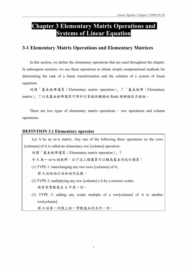
EXAMPLE 1
Let ⎟⎟⎟
⎠
⎞
⎜⎜⎜
⎝
⎛minus=
210431124321
A 經過四種不同型態的運算helliphellip
TYPE 1 Interchanging the second row of A with the first row The result matrix is
⎟⎟⎟
⎠
⎞
⎜⎜⎜
⎝
⎛ minus=
210443213112
B
TYPE 2 Multiplying the second column of A by 3
⎟⎟⎟
⎠
⎞
⎜⎜⎜
⎝
⎛minus=
210431324361
C
TYPE 3 Adding 4 times the third row of A to the first row
⎟⎟⎟
⎠
⎞
⎜⎜⎜
⎝
⎛minus=
21043112
127217M
TYPE 3 Adding -4 times the third row of M to the first row of M A
⎟⎟⎟
⎠
⎞
⎜⎜⎜
⎝
⎛minus=
210431124321
A
Notice that if a matrix Q can be obtained from matrix P by means of an elementary row
operation the P can be obtained from Q by an elementary row operation of the same type
注意若矩陣 Q 經過基本列運算後得到矩陣 P則矩陣 P 亦可由同一 TYPE 的
基本列運算得到矩陣 Q
DEFINITION 32 Elementary matrix
An ntimesn elementary matrix is a matrix obtained by performing an elementary operation
on In The elementart matrix is said to be of type 1 2 or 3 according to whether the
elementary operation performed on In is type 1 2 or 3 operation respectively
「基本矩陣」係指在 In 上實施某一基本運算後所得的矩陣分別在 In 上實施
TYPE 123 基本運算後所得基本矩陣稱為 TYPE 123
Linear Algebra- Chapter 3 20080926
3
For example interchanging the first rows of I3 produces the elementary matrix
⎟⎟⎟
⎠
⎞
⎜⎜⎜
⎝
⎛=
100001010
E 為基本矩陣(Elementary matrix)係由 I3 的前二行互調或前兩列
互調取得
Note that E can be obtained by interchanging the first two columns of I3 In fact any
elementary matrix can be obtained in at least two ways ndash either by performing an elementary
row operation on In or by performing an elementary column operation on In Similarly
⎟⎟⎟
⎠
⎞
⎜⎜⎜
⎝
⎛ minus
100010201
也是基本矩陣(Elementary matrix)此矩陣可由兩種管道取得
is an elementary matrix since it can be obtained from I3 by an elementary column
operation of type 3 (adding -2 times the first column of I3 to the third column)
Theorem 31 Let AisinMmtimesn(F) and suppose that B is obtained from A by performing an elementary
row [column] operation Then there exists an mtimesm [ntimesn] elementary matrix E such that B
= EA [B = AE] IN fact E is obtained from Im [In] by performing the same elementary row
[column[ operation as that which was performed on A to obtain B Conversely if E is an
mtimesm [ntimesn] elementary matrix then EA [AE] is the matrix obtained from A by performing
the same elementary row [column] operation as that which produces E from Im [In]
令 AisinMmtimesn(F)並假設 B 是由 A 經實施某一基本列【或行】運算後所得到的矩
陣則存在一個 mtimesm 【或 ntimesn】基本矩陣 E使得 B = EA【或 B = AE】E 矩陣是
由 Im 【或 In】 經實施與「由 A 得到 B」相同的基本列【或行】運算後所得到的矩
陣反之若 E 是一個 mtimesm【或 ntimesn】的基本矩陣則 EA【或 AE】是由 A 經過與
「由 Im 【或 In】 得到 E」相同的基本列【或行】運算後所得到的矩陣
A Elementary row [column] operations B
Im Elementary row [column] operations E
B = EA [= AE]
Linear Algebra- Chapter 3 20080926
4
EXAMPLE 2 Consider the matrices A and B in Example 1 In this case B is obtained from A by
interchanging the second row of A with the first row Performing this same operation on I3
we obtain the elementary matrix
範例 1A 經過基本列運算(Interchanging the second row of A with the first
row) BIm 經過基本列運算(Interchanging the second row of A with the first
row) E則 B 亦可由 B = EA 取得
⎟⎟⎟
⎠
⎞
⎜⎜⎜
⎝
⎛=
100001010
E ⎟⎟⎟
⎠
⎞
⎜⎜⎜
⎝
⎛minus=
210431124321
A
⎟⎟⎟
⎠
⎞
⎜⎜⎜
⎝
⎛ minus==
210443213112
EAB
Consider the matrices A and C in Example 1 In this case C is obtained from A by
multiplying the second column of A by 3 Performing this same operation on I4 we obtain
the elementary matrix
範例 1A 經過基本行運算(Multiplying the second column of A by 3) C
In 經過基本行運算(Multiplying the second column of A by 3) E則 C 亦可由 C
= AE 取得
⎟⎟⎟⎟⎟
⎠
⎞
⎜⎜⎜⎜⎜
⎝
⎛
=
1000010000300001
E ⎟⎟⎟
⎠
⎞
⎜⎜⎜
⎝
⎛minus=
210431124321
A
C = AE = ⎟⎟⎟
⎠
⎞
⎜⎜⎜
⎝
⎛minus
210431324361
Theorem 32 Elementary matrices are invertible and the inverse of an elementary matrix is an
elementary matrix of the same type
基本矩陣為可逆矩陣且基本矩陣的反矩陣亦是同一型的基本矩陣
【Proof】
Let E be an elementary ntimesn matrix Then E can be obtained by an elementary row
Linear Algebra- Chapter 3 20080926
5
[column] operation on In By reversing the steps used to transform In into E we can
transform E back into In The result is that In can be obtained from E by an elementary row
[column] operation of the same type By Theorem 31 there is an elementary matrix E
such that nIEE = Therefore E is invertible and 1EE minus=
令 E 是 ntimesn 的基本矩陣E 可由 In 經實施一基本列或行運算取得若把用來實
施 In E 的運算對 E 實施亦可得到 In依據 Theorem 31 可知存在一基本矩陣E
使得 nIEE = 因此 E 為可逆且 1EE minus=
Elementary Matrices Elementary Matrices 1414
An elementary matrix is one that can be obtained from the identity matrix In through a single elementary row operation
⎥⎥⎥
⎦
⎤
⎢⎢⎢
⎣
⎡=
100010001
3I⎥⎥⎥
⎦
⎤
⎢⎢⎢
⎣
⎡=
010100001
1ER2 harr R3
⎥⎥⎥
⎦
⎤
⎢⎢⎢
⎣
⎡=
100050001
2E5R25R2
⎥⎥⎥
⎦
⎤
⎢⎢⎢
⎣
⎡=
100012001
3ER2+ 2R1R2+ 2R1
Operation TOperation T
Elementary Matrices Elementary Matrices 2424
⎥⎥⎥
⎦
⎤
⎢⎢⎢
⎣
⎡=
ihgfedcba
A
AEAfedihgcba
1
010100001
=sdot⎥⎥⎥
⎦
⎤
⎢⎢⎢
⎣
⎡=
⎥⎥⎥
⎦
⎤
⎢⎢⎢
⎣
⎡R2 harr R3
AEAihgfed
cba
2
100050001
555 =sdot⎥⎥⎥
⎦
⎤
⎢⎢⎢
⎣
⎡=
⎥⎥⎥
⎦
⎤
⎢⎢⎢
⎣
⎡5R2
AEAihg
cfbeadcba
3
100012001
222 =sdot⎥⎥⎥
⎦
⎤
⎢⎢⎢
⎣
⎡=
⎥⎥⎥
⎦
⎤
⎢⎢⎢
⎣
⎡+++
R2+ 2R1
Elementary Matrices Elementary Matrices 3434
Each elementary matrix is invertible
1221EI
RR +asymp
⎥⎥⎥
⎦
⎤
⎢⎢⎢
⎣
⎡=
100010021
1E
⎥⎥⎥
⎦
⎤
⎢⎢⎢
⎣
⎡=
100010001
I
IE 2R21R1 minus
asymprArr IEE =12 ie
22R21REI
minusasymp
⎥⎥⎥
⎦
⎤
⎢⎢⎢
⎣
⎡ minus=
100010021
E 1
Elementary Matrices Elementary Matrices 4444
If A and B are row equivalent matrices and A is invertible then B is invertibleSince A and B are row equivalent there exits a sequence of row operations T1hellipTn such that B=TnT1ALet the elementary matrices of these operations be E1hellipEn Thus B=En hellip E2 E1 AThe matrix A En hellipE2 E1 are all invertible
( )( )
1
n
1
3
1
2
1
111
11
1n
1
n
1
3
1
2
1
1
1
n
1
3
1
2
1
11
EEEEABBAEE
EEEAEEEEEA
minusminusminusminusminusminus
minusminus
minusminusminusminusminusminusminusminus
=rArr==
=
3-2 The Rank of a Matrix and Matrix Inverse
In this section we define the rank of a matrix We then use elementary operations to
compute the rank of a matrix and a linear transformation The section concludes with a
procedure for computing the inverse of an invertible matrix
何謂「矩陣的秩(Rank)」利用基本行列運算來計算矩陣與線性轉換的秩本節
還包括介紹如何計算可逆矩陣的反矩陣
Linear Algebra- Chapter 3 20080926
6
DEFINITION 33 Rank of a Matrix
If AisinMmtimesn(F) we define the rank of A denoted rank(A) to be the rank of the linear
transformation LA Fn Fm
若 AisinMmtimesn(F)則矩陣 A 的秩為線性轉換 LA Fn Fm的秩註記為 rank(A)
An ntimesn matrix is invertible if and only if its rank is n
一個 ntimesn 的矩陣為可逆的『若且唯若』條件為該矩陣的 Rank 為 n
Every matrix A is the matrix representation of the linear transformation LA with respect
to the appropriate standard ordered bases Thus the rank of the linear transformation LA is the
same as the rank of one of its matrix representation namely A
每一個矩陣 A 是線性轉換 LA 對於某個標準有序基底的矩陣表示式因此該線性轉
換 LA的 Rank 就等於矩陣表示式 A 的 Rank即 rank(LA) = rank(A)
DEFINITION 29
Let V and W be vector spaces and let T V W be linear If N(T) and R(T) are finite-
dimensional then we define the nullity of T denoted nullity(T) and the rank of T denoted
rank(T) to be the dimensions of N(T) and R(T) respectively
V 與 W 為向量空間且 T V W 為線性轉換
定義 T 的核次數(Nullity)nullity(T) = dimensions of N(T)
定義 T 的秩(Rank)rank(T) = dimension of R(T)
核次數(Nullity)與秩(Rank)分別代表 N(T)與 R(T)的維度
DEFINITION 211
Let β = u1 u2hellip un be an ordered basis for a finite-dimensional vectors space V
For xisinV let a1 a2hellip an be the unique scalars such that
令 β = u1 u2hellip un為有限向量空間 V 的有序基底則存在唯一的一組純量 a1
a2hellip an使得 V 內任意向量均可表達成該組基底的線性組合
sum=
=n
1iiiuax
we define the coordinate vector of x relative to β denoted β[x] by
Linear Algebra- Chapter 3 20080926
7
⎟⎟⎟⎟⎟
⎠
⎞
⎜⎜⎜⎜⎜
⎝
⎛
=β
n
2
1
a
aa
[x] 稱為 x 相對於有序基底 β的座標向量
DEFINITION 212
Suppose that V and W are finite-dimensional vector spaces with ordered bases β = v1
v2hellip vn and γ = w1 w2hellip wn respectively Let T V W be linear Then for each j 1
≦j≦n there exist unique scalars aijisinF 1≦i≦m such that
sum==
m
1iiijj wa)vT( for 1≦j≦n
We call the mtimesn matrix A defined by Aij = aij the matrix representation of T in the ordered bases β and γ and write γ
β= [T]A
If V = W and β = γ then we write β= [T]A
設 V 與 W 分別為有限維度的向量空間β = v1 v2hellip vn與 γ = w1 w2hellip
wn分別為 V 與 W 的有序基底且 T V W 為 V 映至 W 的線性轉換
對每一個 j(1≦ j≦n)而言存在唯一的純量 aij isinF(1≦ i≦m)使得
sum==
m
1iiijj wa)vT(
將 mtimesn 的矩陣 A 定義為 Aij = aij並稱呼 A 為線性轉換 T 的矩陣表達方式在
V 與 W 分別以 β 與 γ作為有序基底下A 可註記為 γβ= [T]A
若 V = W 且 β = γ則 β= [T]A
提示 sum==
m
1iiijj wa)vT( 為「將 vj的像 T(vj)表達成有序基底 γ的線性組合」
DEFINITION 217
Let A be an mtimesn matrix with entries from a field F We denote by LA the mapping LA
Fn Fm defined by LA(x) = Ax (the matrix product A and x) for each column vector xisinFn
We call LA a left-multiplication transformation
令 A 是 mtimesn 的矩陣所有元素均來自 FLA為 Fn映至 Fm的線性轉換並定義為
LA(x) = Ax其中 x 為行向量(Column vector)且 xisinFnLA被稱為左乘法轉換
Linear Algebra- Chapter 3 20080926
8
The next theorem extends this fact to any matrix representation of any linear
transformation defined on finite-dimensional vector spaces
Theorem 33 Let T V W be a linear transformation between finite dimensional vector spaces and
let β and γ be ordered bases for V and W respective Then rank(T) = rank( γβ[T] )
令 T V W且 β 與 γ 分別為有限維度向量空間 V 與 W 的有序基底則
rank(T) = rank( γβ[T] )
改寫 Definition 212
Suppose that Fn and Fm are finite-dimensional vector spaces with ordered bases β =
v1 v2hellip vn and γ = w1 w2hellip wn respectively Let LA Fn Fm be linear and defined
by LA(x) = Ax Then for each j 1≦j≦n there exist unique scalars aijisinF 1≦i≦m such
that sum=
=m
1iiijjA wa)v(L for 1≦j≦n We call the mtimesn matrix A defined by Aij = aij the matrix
representation of LA in the ordered bases β and γ and write γβ= ][LA A
Now that the problem of finding the rank of a linear transformation has been reduced to
the problem of finding the rank of a matrix we need a result that allows us to perform rank-
preserving operations on matrices The next theorem and its corollary tell us how to do this
線性轉換的 Rank 可以被簡化為找矩陣的 Rank如何找矩陣的 Rank
Theorem 34 Let A be an mtimesn matrix If P and Q are invertible mtimesm and ntimesn matrices respectively
then
令 A 為 mtimesn 的矩陣若 P 與 Q 分別為可逆的 mtimesm 與 ntimesn 矩陣則
(a) rank(AQ) = rank(A)
(b) rank(PA) = rank(A)
(c) rank(PAQ) = rank(A)
【Proof】
R(LAQ) = R(LALQ) = LALQ(Fn) = LA(LQ(Fn)) = LA(Fn) = R(LA)
Since LQ is onto rank(AQ) = dim(R(LAQ)) = dim(R(LA)) = rank(A)
Linear Algebra- Chapter 3 20080926
9
rank(PAQ) = rank(PA) = rank(A)
註Theorem 34 是為後續 Reduced Row Echelon Form of Matrix 做準備一個矩陣經過
基本行運算或基本列運算或基本行與列運算後並不會改變 RANK
Corollary
Elementary row and column operations on a matrix are rank-preserving
矩陣的基本列與行運算不會改變矩陣的 Rank
此推論結果是計算反矩陣解線性方程組的重要依據
Theorem 35 The rank of any matrix equals the maximum number of its linearly independent
columns that is the rank of a matrix is the dimension of the subspace generated by its
column
任一矩陣的 Rank 等於其最大線性獨立行向量數目即矩陣的 Rank 是由矩陣的
行向量生成的子空間的維度【LA Fn Fm】
【Proof】
For any AisinMmtimesn(F)
rank(A) = rank(LA) = dim(R(LA))
Let β be the standard basis of Fn Then β spans Fn and hence by Theorem 22
R(LA ) = span(LA (β)) = span(LA(e1) LA(e2)hellip LA(en))
But for any j we have seen in Theorem 213(b) that LA(ej) = Aej = aj where aj is the
jth column of A Hence R(LA ) = span(a1 a2 an)
Thus rank(A) = rank(LA) = dim(span(a1 a2 an))
對任意矩陣 Arank(A) = rank(LA) = dim(R(LA))
令 β為 Fn 的標準基底且生成 Fn
依據 Theorem 22
LA的值域 Range 可由 LA(β)來生成
R(LA) = span(LA (β)) = span(LA(e1) LA(e2)hellip LA(en))
對任意 j 而言由 Theorem 213(b) 可知 LA(ej) = Aej = aj其中aj 為 A 的第 j
個行(aj 相當於 Theorem 213(b)的 vj 或 Theorem 22 的 T(vj))因此 R(LA) =
Linear Algebra- Chapter 3 20080926
10
span(a1 a2 an)
所以 rank(A) = rank(LA) = dimension of R(LA) = dim(span(a1a2an))
Theorem 22 令 V 與 W 為向量空間且 T V W 為線性轉換若 β = v1 v2hellip vn
是定義域(Domain)V 的基底則 T 的值域 Range R(T)可由 T(β)來生成意即 R(T)
= span(T(β)) = span(T(v1) T(v2)hellip T(vn))
Theorem 213 A 為 mtimesn 的矩陣與 B 為 ntimesp 的矩陣uj 與 vj分別為 AB 與 B 的第 j 行
(1 j p≦ ≦ )則
(a) uj = A vj
(b) vj = B ej where ej is the jth standard vector of Fp
EXAMPLE 1
Let ⎟⎟⎟
⎠
⎞
⎜⎜⎜
⎝
⎛=
101110101
A
Observe that the first and second columns of A are linearly independent and that the
third column is a linear combination of the first two Thus
A 的第一行與第二行是線性獨立第三行則是前兩行的線性組合於是
rank(A) = dim⎟⎟⎟⎟
⎠
⎞
⎜⎜⎜⎜
⎝
⎛
⎟⎟⎟
⎠
⎞
⎜⎜⎜
⎝
⎛
⎪⎭
⎪⎬
⎫
⎟⎟⎟
⎠
⎞
⎜⎜⎜
⎝
⎛
⎪⎩
⎪⎨
⎧
⎟⎟⎟
⎠
⎞
⎜⎜⎜
⎝
⎛
⎟⎟⎟
⎠
⎞
⎜⎜⎜
⎝
⎛
111
010
101
span = 2
A 的第 1 行a1=⎟⎟⎟
⎠
⎞
⎜⎜⎜
⎝
⎛
101第 2 行a2=
⎟⎟⎟
⎠
⎞
⎜⎜⎜
⎝
⎛
010第 3 行a3=
⎟⎟⎟
⎠
⎞
⎜⎜⎜
⎝
⎛
111
In order to compute the rank of a matrix A it is frequently useful to postpone the use of
Theorem 35 until A has been suitable modified by means of appropriate elementary row and
column operations so that the number of linearly independent columns is obvious
為了利用 Theorem 35 求矩陣 A 的 Rank(等於最大線性獨立行向量數目)A 可
先經過基本列或行運算使其線性獨立的行數變得比較明顯
EXAMPLE 2 Let
Linear Algebra- Chapter 3 20080926
11
⎟⎟⎟
⎠
⎞
⎜⎜⎜
⎝
⎛=
211301121
A
If we subtract the first row of A from rows 2 and 3 (type 3 elementary row operations)
the result is
⎟⎟⎟
⎠
⎞
⎜⎜⎜
⎝
⎛
minusminus
110220121
If we now substract twice the first column from the second and substract the first
column from the third (type 3 elementary column operations) we obtain
⎟⎟⎟
⎠
⎞
⎜⎜⎜
⎝
⎛
minusminus
110220001
(後二行線性相依最大線性獨立行數為 2)
It is now obvious that the maximum number of linearly independent column of this matrix is 2 Hence the rank of A is 2
Theorem 36 Let A be an mtimesn matrix of rank r Then r m r n and by means of a finite number ≦ ≦
of elementary row and column operations A can be transformed into the matrix
D = ⎟⎟⎠
⎞⎜⎜⎝
⎛
32
1r
OOOI
where O1 O2 and O3 are zero matrices Thus Dii = 1 for i r and ≦
Dij = 0 otherwise
令 A 為 Rank 等於 r 的 mtimesn 矩陣則 r m≦ 且 r n≦ 經過有限次數的基本行與列
運算讓 A 化成 D = ⎟⎟⎠
⎞⎜⎜⎝
⎛
32
1r
OOOI
其中Ir 為對角元素為 1 的對角矩陣即 A 可經
過有限次數的基本行及列運算取得沿對角線前 r 個位置皆為 1其餘各處皆為 0 的
矩陣 D
【Proof】
If A is the zero matrix r = 0 In this case the conclusion follows with D = A
若 A 為零矩陣則 r = 0 且 D = A
Now suppose that AneO and r = rank(A) then r gt 0
The proof is by mathematical induction on m the number of rows of A
若 A 非零矩陣且 r = rank(A)則 r gt 0
Linear Algebra- Chapter 3 20080926
12
採用數學歸納法
Suppose that m = 1
A can be transformed into the matrix (1 0 hellip0)
So rank(D) = rank(A) = 1 by Corollary to Theorem 34 and Theorem 35 Thus the
theorem is established for m = 1
設 m = 1則 A 可以化成(1 0 hellip0)
依據 Corollary to Theorem 34 及 Theorem 35
rank(D) = rank(A) = 1
故本定理對 m = 1 的矩陣是成立的
Next assume that the theorem holds for any matrix with at most m - 1 row (for some m
gt1)
We must prove that the theorem holds for any matrix with m rows
其次假設本定理對至多含 m - 1 列的矩陣皆成立(m gt 1)
至於含 m 列的矩陣是否成立
If n = 1 Theorem 36 can be established in a manner analogous to that for m = 1
若 n = 1則可按 m = 1 的方式證明本定理對於 n = 1 的矩陣成立
We now suppose that n gt 1 Since A ne O Aijne0 for some i j By means of at most one
elementary row and at most one elementary column operation (each of type 1) We can
move the nonzero entry to the 11 position By means of of at most one additional type 2
operation we can assure a 1 in the 11 position By means of at most m ndash 1 type 3 row
operations and at most n ndash 1 type 3 column operations we can eliminate all nonzero entries
in the first row and the first column with the exception of the 1 in the 11 postion
Thus with a finite number of elementary operation A can be transformed into a
matrix
經過有限次數的基本行及列運算可將 A 轉換成
⎪⎪⎭
⎪⎪⎬
⎫
⎪⎪⎩
⎪⎪⎨
⎧
=
0B
0001
B where Brsquo is an (m-1)times(n-1) matrix
Brsquo has rank one less than B
Brsquo的 Rank 比 B 少 1
Since rank(A) = rank(B) = r rank(Brsquo) = r ndash 1 Therefore r ndash1 ≦ m ndash 1 and r ndash1 ≦
Linear Algebra- Chapter 3 20080926
13
n ndash 1 by the induction hypothesis Hence r ≦ m and r ≦ n
由於 rank(A) = rank(B) = r故 rank(Brsquo) = r ndash 1
依數學歸納法 r ndash1 ≦ m ndash 1 且 r ndash1 ≦ n ndash 1
因此 r ≦ m 且 r ≦ n
Also by the induction hypothesis Brsquo can be transformed by a finite number of
elementary row and column operations into the (m-1)times(n-1) matrix Drsquo such that
同樣地依據數學歸納法Brsquo 可經過有限次數的基本行與列運算轉換成 (m-
1)times(n-1) 的矩陣 Drsquo使得
Dlsquo= ⎟⎟⎠
⎞⎜⎜⎝
⎛ minus
65
41r
OOOI
where O4 O5 and O6 are zero matrices
That is Drsquo consists of all zeros except for its first r-1 diagonal entries which are ones
Let
⎪⎪⎭
⎪⎪⎬
⎫
⎪⎪⎩
⎪⎪⎨
⎧
=
0D
0001
D
We see that the theorem now follows once we show that D can be obtained from B by
means of a finite number of elementary row and column operations
D 可由 B 經過有限次基本行及列運算而取得
Thus since A can be transformed into B and B can be transformed into D each by a
finite number of elementary operations A can be transformed into D by a finite number of
elementary operations
經過有限次基本行及列運算A B D
Finally since Drsquo contains ones as its first r ndash 1 diagonal entries D contains ones as its
first r diagonal entries and zeros elsewhere
最後Drsquo沿對角線前 r-1 個位置皆為 1故 D 沿對角線前 r 個位置皆為 1其餘
各處皆為 0
EXAMPLE 3 Consider the maxtrix
⎟⎟⎟⎟⎟
⎠
⎞
⎜⎜⎜⎜⎜
⎝
⎛
=
192362100280844422420
A
Linear Algebra- Chapter 3 20080926
14
By means of a succession of elementary row and column operations we can transform
A into a matrix D as in Theorem 36
透過一系列的基本行與列運算將 A 轉換成 D
D
00000001000001000001
192362100280844422420
A =
⎟⎟⎟⎟⎟
⎠
⎞
⎜⎜⎜⎜⎜
⎝
⎛
==
⎟⎟⎟⎟⎟
⎠
⎞
⎜⎜⎜⎜⎜
⎝
⎛
=
By the corollary to Theorem 34 rank(A) = rank(D) Clearly however rank(D) = 3 so rank(A) = 3
Corollary 1 Let A be an mtimesn matrix of rank r Then there exist invertible matrices B and C of sizes
mtimesm and ntimesn respectively such that D = BAC where D = ⎟⎟⎠
⎞⎜⎜⎝
⎛
32
1r
OOOI
is the mtimesn matrix
in which O1 O2 and O3 are zero matrices
令 A 為 mtimesn 的矩陣Rank 為 r存在可逆的 mtimesm 矩陣 B 與 ntimesn 矩陣 C使得
D = BAC其中D = ⎟⎟⎠
⎞⎜⎜⎝
⎛
32
1r
OOOI
為 mtimesn 的矩陣O1O2 及 O3 為零矩陣
【Proof】
By Theorem 36 A can be transformed by means of a finite number of elementary
row and column operations into the matrix D
We can appeal to Theorem 31 each time we perform an elementary operation Thus
there exist elementary mtimesm matrices E1 E2hellipEp and elementary ntimesn matrices G1
G2hellipGq such that D = EpEp-1hellipE2E1AG1G2hellipGq
By Theorem 32 each Ej and Gj is invertible Let B = EpEp-1hellipE2E1 and C =
G1G2hellipGq Then B and C are invertible and D = BAC
依據 Theorem 36A 可經過有限次的基本列與行運算化成 D
引用 Theorem 31每一次皆實施某一個基本列運算於是存在基本的 mtimesm 矩
陣 E1 E2hellip Ep 與 基 本 的 ntimesn 矩 陣 G1 G2hellip Gq 使 得 D = EpEp-
1hellipE2E1AG1G2hellipGq
依據 Theorem 32 每一個基本矩陣 Ej與 Gj 皆為可逆令 B = EpEp-1hellipE2E1 與 C =
G1G2hellipGq於是 B 與 C 皆為可逆且 D = EpEp-1hellipE2E1AG1G2hellipGq = BAC
Linear Algebra- Chapter 3 20080926
15
Theorem 31 令 AisinMmtimesn(F)並假設 B 是由 A 經實施某一基本列【或行】運算後所得
到的矩陣則存在一個 mtimesm 【或 ntimesn】基本矩陣 E使得 B = EA【或 B = AE】E
矩陣是由 Im 【或 In】 經實施與「由 A 得到 B」相同的基本列【或行】運算後所得
到的矩陣反之若 E 是一個 mtimesm【或 ntimesn】的基本矩陣則 EA【或 AE】是由 A
經過與「由 Im 【或 In】 得到 E」相同的基本列【或行】運算後所得到的矩陣
Theorem 32 基本矩陣為可逆矩陣且基本矩陣的反矩陣亦是同一型的基本矩陣
Theorem 36 令 A 為 Rank 等於 r 的 mtimesn 矩陣則 r m≦ 且 r n≦ 經過有限次數的基
本行與列運算讓 A 化成 D = ⎟⎟⎠
⎞⎜⎜⎝
⎛
32
1r
OOOI
其中Ir為對角元素為 1 的對角矩陣
Corollary 2 Let A be an mtimesn matrix Then
(a) rank(At) = rank(A)
矩陣轉置後的 RANK 不變
(b) The rank of any matrix equals the maximum number of its linearly independent
rows that is the rank of a matrix is the dimension of the subspace generated by
rows
任一矩陣的 Rank 等於最大線性獨立列向量的數目即矩陣的 Rank 等於由該
矩陣列向量所生成的子空間的維度
(c) The rows and columns of any matrix generate subspaces of the same dimension
numerically equal to the rank of the matrix
任一矩陣的列向量與行向量生成的子空間的維度相同維度等於該矩陣的
Rank
【Proof】
By Corollary 1 there exist invertible matrices B and C such that D = BAC where D
satisfies the stated conditions of the corollary Taking transposes we have
Dt = (BAC) t = CtAtBt
Since B and C are invertible so are Bt and Ct
Hence by Theorem 34 rank(At) = rank(CtAtBt) = rank(Dt)
Suppose that r = rank(A)
Then Dt is an ntimesm matrix with the form of the matrix D in Corollary 1 and hence
Linear Algebra- Chapter 3 20080926
16
rank(Dt) = r by Theorem 35
Thus
rank(At) = rank(Dt) = r = rank(A)
依據 Corollary 1存在可逆矩陣 B 與 C使得 D = BAC
取其轉置可得Dt = (BAC) t = CtAtBt
由於 B 與 C 為可逆故 Bt 與 Ct 亦為可逆
依據 Theorem 34得知 rank(At) = rank(CtAtBt) = rank(Dt)
設 r = rank(A)
則 Dt為一 ntimesm 的矩陣型式與 D 相同(參考 Corollary 1)
且依據 Theorem 35 得知 rank(Dt) = r
於是 rank(At) = rank(Dt) = r = rank(A)
Theorem 34 Let A be an mtimesn matrix If P and Q are invertible mtimesm and ntimesn matrices
respectively then 令 A 為 mtimesn 的矩陣若 P 與 Q 分別為可逆的 mtimesm 與 ntimesn 矩陣
則
(a) rank(AQ) = rank(A)
(b) rank(PA) = rank(A)
(c) rank(PAQ) = rank(A)
Theorem 35 The rank of any matrix equals the maximum number of its linearly
independent columns that is the rank of a matrix is the dimension of the subspace
generated by its column 任一矩陣的 Rank 等於其最大線性獨立行向量數目即矩陣
的 Rank 是由矩陣的行向量生成的子空間的維度【LA Fn Fm】
Corollary 3 Every invertible matrix is a product of elementary matrices
每一可逆矩陣均可為基本矩陣的乘積
【Proof】
If A is an invertible ntimesn matrix then rank(A) = n Hence the matrix D in Corollary 1
equals In and there exist invertible matrices B and C such that In = BAC
As in the proof of Corollary 1 note that B = EpEp-1hellipE2E1 and C = G1G2hellipGq where
the Eirsquos and Girsquos are elementary matrices Thus A = B-1InC-1 = B-1C-1 so that
A = E1-1E2
-1hellipEp-1Gq
-1Gq-1-1hellipG1
-1
Linear Algebra- Chapter 3 20080926
17
The inverses of elementary matrices are elementary matrices however and hence A is
the product of elementary matrices
若 A 為可逆的 ntimesn 矩陣則 rank(A) = n
因此 Corollary 1 中的矩陣 D 為 In且存在可逆的 B 與 C 矩陣使得 In = BAC
如同 Corollary 1 的證明一樣B = EpEp-1hellipE2E1 且 C = G1G2hellipGq其中Eirsquos 與
Girsquos 皆為基本矩陣
於是A = B-1InC-1 = B-1C-1即 A = E1-1E2
-1hellipEp-1Gq
-1Gq-1-1hellipG1
-1
基本矩陣的反矩陣亦為基本矩陣A 是基本矩陣的乘積
Theorem 37 Let T V W and U W Z be linear transformations on finite-dimensional vector
spaces V W and Z and let A and B be matrices such that the product AB is defined Then
令 VW 與 Z 為有限維度的向量空間T V W 與 U W Z 為線性轉換且
A 與 B 為滿足乘積 AB 定義的矩陣則
(a) rank(UT) ≦ rank(U)
(b) rank(UT) ≦ rank(T)
(c) rank(AB) ≦ rank(A)
(d) rank(AB) ≦ rank(B)
【Proof】
(a) Clearly R(T)subeW
Hence R(UT) = UT(V) = U(R(T)) sube U(W) = R(U)
Thus rank(UT) = dim(R(UT)) ≦ dim (R(U)) = rank(U)
(c) By (a) rank(AB) = rank(LAB) = rank (LALB) ≦ rank(LA) = rank(A)
(d) By (c) and Corollary 2 to Theorem 36
rank(AB) = rank((AB)t) = rank(B t A t) ≦ rank(B t) = rank (B) (b) Let α β and γ be ordered bases for V W and Z respectively and let Arsquo = γ
β]U[
and Brsquo = βα]T[ Then ArsquoBrsquo = γ
α]UT[ by Theorem 211
Hence by Theorem 33 and (d)
rank(UT) = rank(ArsquoBrsquo) ≦ rank(Brsquo) = rank (T)
Theorem 211 Let V W and Z be finite-dimensional vector space with ordered bases α β
and γ respectively Let T V W and U W Z be linear transformation Then
Linear Algebra- Chapter 3 20080926
18
βα
γβ
γα = [T][U][UT] 令 VW 與 Z 是有限維度的向量空間αβ 與 γ 分別為 VW 與
Z 的有序基底令 T V W (先 α β) 且 U W Z (後 β γ)則 βα
γβ
γα = [T][U][UT]
Theorem 33 Let T V W be a linear transformation between finite dimensional vector
spaces and let β and γ be ordered bases for V and W respective Then rank(T) = rank( γ
β[T] ) 令 T V W且 β 與 γ 分別為有限維度向量空間 V 與 W 的有序基底
則 rank(T) = rank( γβ[T] )
EXAMPLE 4
(a) Let ⎟⎟⎠
⎞⎜⎜⎝
⎛minus
=11111121
A (第一列與第二列是 LI) rank(A) = 2
(b) Let ⎟⎟⎟
⎠
⎞
⎜⎜⎜
⎝
⎛=
003011011131
A (第三列與第一二列是 LD)rank(A) = 2
(c) Let ⎟⎟⎟
⎠
⎞
⎜⎜⎜
⎝
⎛
minus=
011111121321
A (三列為 LI) rank(A) = 3
The inverse of a Matrix
We have remarked that an ntimesn matrix is invertible if and only if its rank is n Since we
know how to compute the rank of any matrix we can always test a matrix to determine
whether it is invertible We now provide a simple technique for computing the inverse of a
matrix that utilizes elementary row operations
已知 ntimesn 矩陣為可逆的『若且唯若』條件為該矩陣的 Rank 等於 n
DEFINITION 34 Augmented Matrix Let A and B be mtimesn and mtimesp matrices respectively By the augmented matrix )BA(
we mean that the mtimes(n+p) matrix )BA( that is the matrix whose first n columns are the
columns of A and whose last p columns are the columns of B 設 A 與 B 分別為 mtimesn 與 mtimesp 的矩陣則增廣矩陣(Augmented matrix) )BA(
Linear Algebra- Chapter 3 20080926
19
為一 mtimes(n+p)的矩陣 )BA( 該矩陣的前 n 行(Column)為 A 的所有的行後 p
行為 B 的所有行
Let A be an invertible ntimesn matrix and consider the ntimes2n augmented matrix C= )IA( n
C= )IA( n )AI()IAAA(CA 1
nn111 minusminusminusminus ==
By Corollary 3 to Theorem 36 A-1 is the product of elementary matrices say
A = EpEp-1hellipE2E1 (A-1 是多個基本矩陣的乘積)
Thus )AI()IAAA(CA 1
nn111 minusminusminusminus == )AI(CA)IA(EEE 1
n1
n11ppminusminus
minus ==
We have the following result If A is an invertible invertible ntimesn matrix then it is
possible to transform the matrix (AIn) into the matrix (InA-1) by means of a finite
number of elementary row operations
若 A 為一可逆的 ntimesn 矩陣則可經過有限次數的基本列運算將矩陣 (AIn) 化成
(InA-1)
Conversely suppose that A is invertible and that for some ntimesn matrix B the matrix
(AIn) can be transformed into the matrix (InB) by a finite number of elementary row
operations Let E1 E2hellip Ep be the elementary matrices associated with these elementary row
operations as in Theorem 31 then
反之假設 A 是可逆且矩陣(AIn)可經有限次數的基本列運算轉換成矩陣(InB)
並令 E1 E2hellip Ep 分別為 Theorem 31 所稱的基本矩陣則
)BI()IA(EEE nn11pp =minus
Let M = EpEp-1hellipE2E1 we have 令 M = EpEp-1hellipE2E1
)BI()IA(EEE nn11pp =minus )BI()IA(M)MMA( nn ==
Linear Algebra- Chapter 3 20080926
20
Hence MA = In and M = B It follows that M = A-1 So B = A-1
可由 MA = In 及 M = B 得知M 就是 A-1故 B 就是 A-1
Thus we have the follow resultsIf A is an invertible ntimesn matrix and the matrix
(AIn) is transformed in a matrix of the form (InB) by means of a finite number of
elementary row operations then B=A-1
若 A 為一可逆的 ntimesn 矩陣且矩陣 (AIn) 可經有限次數的基本列運算化成
(InB)則 B=A-1
If on the other hand A is an ntimesn matrix that is not invertible then rank(A) lt n Hence
any attempt to transform (AIn) into a matrix of the form (InB) by means of elementary row
operations must fail
反之若 A 是一不可逆的 ntimesn 矩陣則 rank(A) lt n因此任何想利用基本列運算
要將矩陣 (AIn) 化成 (InB)的努力必定失敗
Thus we have the follow results If A is an notinvertible ntimesn matrix then any attempt
to transform (AIn) into a matrix of the form (InB) produce a row whose first n entries
are zeros
若 A 是一不可逆的 ntimesn 矩陣任何想將矩陣 (AIn) 化成 (InB)的努力最後會
產生一前 n 個元素均為 0 的列
EXAMPLE 5
We determine whether the matrix ⎟⎟⎟
⎠
⎞
⎜⎜⎜
⎝
⎛=
133242420
A is invertible and if it is we
compute its inverse
A 是否為可逆矩陣
We attempt to use elementary row operations to transfer
Linear Algebra- Chapter 3 20080926
21
⎟⎟⎟
⎠
⎞
⎜⎜⎜
⎝
⎛=
100010001
133242420
)IA( into a matrix of the form (InB)
看看能否利用基本行與列運算將矩陣 (AIn) 化成 (InB)
Interchanging rows 1 and 2
⎟⎟⎟
⎠
⎞
⎜⎜⎜
⎝
⎛
100001010
133420242
Multiplying the first row by 12
⎟⎟⎟
⎠
⎞
⎜⎜⎜
⎝
⎛
10000100
133420121 2
1
Adding -3 times row 1 to row 3
⎟⎟⎟
⎠
⎞
⎜⎜⎜
⎝
⎛
minusminusminus 1000100
230420121
23
21
Multiplying row 2 by 12 to obtain 1 in the 22 position
⎟⎟⎟
⎠
⎞
⎜⎜⎜
⎝
⎛
minus
minus
minusminus 100000
230210121
23
21
21
Adding -2 times row 2 to row 1 and 3 times row 2 to row 3
⎟⎟⎟
⎠
⎞
⎜⎜⎜
⎝
⎛
minus
minusminus
10001
400210301
23
2321
21
Multiplying row 3 by 14
⎟⎟⎟
⎠
⎞
⎜⎜⎜
⎝
⎛
minus
minusminus
41
83
8321
21
0001
100210301
Adding appropriate multiply of row 3 to row 1 and 2 completes the process
⎟⎟⎟
⎠
⎞
⎜⎜⎜
⎝
⎛
minusminus
minus
41
83
83
21
43
41
43
85
81
100010001
目標達成
Thus A is invertible and ⎟⎟⎟
⎠
⎞
⎜⎜⎜
⎝
⎛
+minus+minus+minus+minus+
=minus
41
83
83
21
43
41
43
85
81
1A
Linear Algebra- Chapter 3 20080926
22
EXAMPLE 6
We determine whether the matrix ⎟⎟⎟
⎠
⎞
⎜⎜⎜
⎝
⎛minus=451112
121A is invertible and if it is we
compute its inverse
A 是否為可逆矩陣
We attempt to use elementary row operations to transfer
⎟⎟⎟
⎠
⎞
⎜⎜⎜
⎝
⎛minus=
100010001
451112
121)IA( into a matrix of the form (InB)
看看能否利用基本行與列運算將矩陣 (AIn) 化成 (InB)
Adding -2 times row 1 to row 2 and -1 times row 1 to row 3 then addig row 2 to row
3
⎟⎟⎟
⎠
⎞
⎜⎜⎜
⎝
⎛minus
100010001
451112
121
⎟⎟⎟
⎠
⎞
⎜⎜⎜
⎝
⎛
minusminusminusminus
101012001
330330
121
⎟⎟⎟
⎠
⎞
⎜⎜⎜
⎝
⎛
minusminusminusminus
113012001
000330
121
is a matrix with row whose first 3 entries are zeros Therefore A is not invertible
最後一列前 3 個元素均為 0
EXAMPLE 7 Let T P2(R) P2(R) be defined by T(f(x)) = f(x)+frsquo(x)+frdquo(x) where frsquo(x) and frdquo(x)
denote the first and second derivatives of f(x) We use Corollary 1 to Theorem 218 to test
T for invertibility and compute the inverse if T is invertible Taking β=1 x x2 to be the
standard ordered basis of P2(R) we have
令 T P2(R) P2(R) 為線性轉換且定義為 T(f(x)) = f(x)+frsquo(x)+frdquo(x)利用
Corollary 1 to Theorem 218 來測試 T 是否可逆並計算其逆轉換取 β=1 x x2為
P2(R)的標準有序基底
T(1) = 1 = 1bull1+0bullx+0bullx2
T(x) = 1+x = 1bull1+1bullx+0bullx2
Linear Algebra- Chapter 3 20080926
23
T(x2) = 2+2x+x2 = 2bull1+2bullx+1bullx2
⎟⎟⎟
⎠
⎞
⎜⎜⎜
⎝
⎛=β
100210211
[T] 稱為 T 相對有序基底 β的座標向量
依據 Corollary 1 to Theorem 218 T 可逆『若且唯若』 β[T] 可逆且
1-1 )[T](][T minusββ =
Using the method of Examples 5 and 6 we can show that β[T] is invertible with
inverse
⎟⎟⎟
⎠
⎞
⎜⎜⎜
⎝
⎛minus
minus=minus
β
100210
011)([T] 1
Thus T is is invertible and βminusminus
β = ][T)([T] 11 Hence by Theorem 214 we have
⎟⎟⎟
⎠
⎞
⎜⎜⎜
⎝
⎛minusminus
=⎟⎟⎟
⎠
⎞
⎜⎜⎜
⎝
⎛
⎟⎟⎟
⎠
⎞
⎜⎜⎜
⎝
⎛minus
minus=++ β
minus
2
21
10
2
1
02
2101
aa2aaa
aaa
100210
011)]xaxa(a[T
Therefore T-1(a0+a1x+a2x2) = (a0-a1)+(a1-2a2)x+a2x2 Corollary 1 to Theorem 218 Let V be finite-dimensional vector space with an ordered basis β and let T V V be linear Then T is invertible if and only if β[T] is invertible
Furthermore 1-1 )[T](][T minusββ = V 為有限維度的向量空間β 是 V 的有序基底令 T
V V 為線性轉換 T 為可逆的『若且唯若』條件為 β[T] 可逆再者
1-1 )[T](][T minusββ =
Theorem 214 Let V and W be finite-dimensional vector spaces having ordered bases β and γ respectively and let T V W be linear Then for each uisinV we have β
γβγ = [u][T][T(u)]
V 與 W 為有限維度的向量空間β 與 γ分別 V 與 W 的有序基底令 T V W 為線
性轉換則 V 中的 u 映至 W 的結果 T(u) 相對於有序基底 γ 的座標向量為
βγβγ = [u][T][T(u)]
Invertible and Inverse of MATRIX Let A be an n times n matrix If a matrix B can be found such that AB = BA = In then A is
Linear Algebra- Chapter 3 20080926
24
said to be invertible and B is called the inverse of A (denote B = A-1 and A-k=(A-1)k )
If such a matrix B does not exist then A has no inverse
EXAMPLE
⎥⎦
⎤⎢⎣
⎡=
4321
A and ⎥⎦
⎤⎢⎣
⎡minus
minus=
21
23
12B
221
23
221
23
I1001
432112
BA
I100112
4321
AB
=⎥⎦
⎤⎢⎣
⎡=⎥
⎦
⎤⎢⎣
⎡⎥⎦
⎤⎢⎣
⎡minus
minus=
=⎥⎦
⎤⎢⎣
⎡=⎥
⎦
⎤⎢⎣
⎡minus
minus⎥⎦
⎤⎢⎣
⎡=
Thus AB = BA = I2 proving that the matrix A has inverse B
Theorem The inverse of an invertible matrix is unique
Let B and C be inverse of A
Thus AB = BA = In and AC = CA = In
Multiply both sides of the equation AB = In by C
C(AB) = CIn (CA)B = C
InB = C B = C
Thus an invertible matrix has only one inverse
How to find AHow to find A--11
Based on the GaussBased on the Gauss--Jordan algorithmJordan algorithmLet A be an invertible matrix Then AALet A be an invertible matrix Then AA--11=I=Inn
Let the columns of Let the columns of AA--11 be be XX11 XX22 helliphellip XXnn and the columns of I and the columns of Inn be be CC11CC22helliphellipCCnn
Find AFind A--11 by finding by finding XX11 XX22 helliphellip XXnn Write the equation AAWrite the equation AA--11=I=Inn in the formin the form
[ ] [ ]n21nn211 CCCI XXXALet LL ==minus
[ ] [ ][ ] [ ]n21n21
n21n21
CCCAXAXXACCCXXXALL
LL
=rArr=
nn2211 CAXCAX CAX === LThus
How to find AHow to find A--11
Solving these systems by using Gauss-Jordan elimination on the large augmented matrix [AC1 C2hellipCn]
Thus when A-1 exits
[ ] [ ] [ ] 1n
1nn ABwhereBIAIIA minusminus ==asympasympL
If the reduced echelon form of [If the reduced echelon form of [AIAInn] is computed and ] is computed and the first part is not of the form Ithe first part is not of the form Inn then A has no inversethen A has no inverse
[ ][ ]n21n
n21
XXXI CCCAmatrix augmented
LL
L
asympasymp
Linear Algebra- Chapter 3 20080926
25
Example Example 1212
⎥⎥⎥
⎦
⎤
⎢⎢⎢
⎣
⎡
minusminusminusminusminus
=100531010532001211
]IA[ 3
⎥⎥⎦
⎤
⎢⎢⎣
⎡minusminusminus
minusminus
+minus+
asymp
101320012110001211
1RR1R3
2)(R2
⎥⎥⎦
⎤
⎢⎢⎣
⎡minus
minusminusminusasymp
101320012110001211
R2)1(
⎥⎥⎥
⎦
⎤
⎢⎢⎢
⎣
⎡
minusminusminusminusminus
=531532211
ADetermine the inverse of
Example Example 2222
⎥⎥⎦
⎤
⎢⎢⎣
⎡
minusminusminusminus
minus++asymp
123100012110013101
R2)2(R3R2R1
⎥⎥⎦
⎤
⎢⎢⎣
⎡
minusminusminus
minus++asymp
123100135010010001
R3)1(R2R3R1
123135110
A 1
⎥⎥⎥
⎦
⎤
⎢⎢⎢
⎣
⎡
minusminusminus=minus
⎥⎥⎦
⎤
⎢⎢⎣
⎡
minusminus
minus
+minus+asymp
135000011210012301
3R2R3R2)1(R1
ExampleExampleDetermine the inverse of
⎥⎥⎦
⎤
⎢⎢⎣
⎡
minus=
412721511
A
⎥⎥⎦
⎤
⎢⎢⎣
⎡
minus=
100412010721001511
][ 3IA
⎥⎥⎦
⎤
⎢⎢⎣
⎡
minusminusminusminus
minus+minus+asymp
102630011210001511
R1)2(R31)R1(R2
There is no need to proceed further There is no need to proceed further The reduced echelon form cannot have a one in the (3 3) locatioThe reduced echelon form cannot have a one in the (3 3) location n
The reduced echelon form cannot be of the form [IThe reduced echelon form cannot be of the form [Inn B] B] Thus Thus AAndashndash11 does not existdoes not exist
Properties of Matrix InverseProperties of Matrix Inverse
Let Let AA and and BB be invertible matrices andbe invertible matrices and cc a nonzero scalar a nonzero scalar ThenThen
AA =minusminus 11)( 111 1)( 2 minusminus = A
ccA
111)( 3 minusminusminus = ABAB
nn AA )()( 4 11 minusminus =tt AA )()( 5 11 minusminus =
Color Models Color Models 1212
A color model in the context of graphics is a method of A color model in the context of graphics is a method of implementing colorsimplementing colorsThe common used models include RGB model and YIQ modelThe common used models include RGB model and YIQ modelThe RGB model is used in computer monitors and the YIQ model The RGB model is used in computer monitors and the YIQ model is used in television screensis used in television screensAn RGB computer signal can be converted to a YIQ television An RGB computer signal can be converted to a YIQ television signal using the matrix transformationsignal using the matrix transformation
⎥⎥⎥
⎦
⎤
⎢⎢⎢
⎣
⎡
⎥⎥⎥
⎦
⎤
⎢⎢⎢
⎣
⎡
minusminusminus=
⎥⎥⎥
⎦
⎤
⎢⎢⎢
⎣
⎡
BGR
311523212321275596
114587299
QIY
YIQgtRGBYIQgtRGB
Color Models Color Models 2222
A signal is converted from a television screen to a computer monA signal is converted from a television screen to a computer monitor itor using inverse of the above matrixusing inverse of the above matrix
⎥⎥⎥
⎦
⎤
⎢⎢⎢
⎣
⎡
⎥⎥⎥
⎦
⎤
⎢⎢⎢
⎣
⎡
minusminusminus=
⎥⎥⎥
⎦
⎤
⎢⎢⎢
⎣
⎡rArr
⎥⎥⎥
⎦
⎤
⎢⎢⎢
⎣
⎡
⎥⎥⎥
⎦
⎤
⎢⎢⎢
⎣
⎡
minusminusminus=
⎥⎥⎥
⎦
⎤
⎢⎢⎢
⎣
⎡minus
QIY
0751108116472721
6209561
BGR
QIY
311523212321275596
114587299
BGR 1
CryptographyCryptography 密碼學密碼學 1212
Cryptography is the process of coding and decoding messagesCryptography is the process of coding and decoding messagesThe technique can be traced back to the ancient Greeks Today The technique can be traced back to the ancient Greeks Today governments use sophisticated methods of coding and decoding governments use sophisticated methods of coding and decoding messagesmessagesOne type of code that is extremely difficult to break makes use One type of code that is extremely difficult to break makes use of a of a large matrix to encode a message large matrix to encode a message The receiver of the message decodes it using the inverse of the The receiver of the message decodes it using the inverse of the matrixmatrixThe first matrix is called the encoding matrix and its inverse The first matrix is called the encoding matrix and its inverse is is called the decoding matrixcalled the decoding matrix
Cryptography Cryptography 密碼學密碼學 2222
A A-1Message
Encoding MatrixEncoding Matrix
Decoded MessageTransmission
Decoding MatrixDecoding Matrix
Linear Algebra- Chapter 3 20080926
26
Example Example 1212
Let the message be Let the message be BUY IBM STOCKBUY IBM STOCKAnd the encoding matrix beAnd the encoding matrix be
⎥⎥⎥
⎦
⎤
⎢⎢⎢
⎣
⎡ minusminusminus
434110433
B U Y B U Y -- I B M I B M -- S T O C KS T O C K2 21 25 27 9 2 13 27 19 20 15 3 112 21 25 27 9 2 13 27 19 20 15 3 11
⎥⎥⎥
⎦
⎤
⎢⎢⎢
⎣
⎡ minusminusminusminusminus=
⎥⎥⎥
⎦
⎤
⎢⎢⎢
⎣
⎡
⎥⎥⎥
⎦
⎤
⎢⎢⎢
⎣
⎡ minusminusminus
2331372091431715418461146
222117196116169
27319225271527921112013272
434110433
EncodingEncoding
Example Example 2222
Let the message be Let the message be BUY IBM STOCKBUY IBM STOCKAnd the decoding matrix beAnd the decoding matrix be
⎥⎥⎥
⎦
⎤
⎢⎢⎢
⎣
⎡
minusminus 334344101
B U Y B U Y -- I B M I B M -- S T O C KS T O C K2 21 25 27 9 2 13 27 19 20 15 3 112 21 25 27 9 2 13 27 19 20 15 3 11
⎥⎥⎥
⎦
⎤
⎢⎢⎢
⎣
⎡=
⎥⎥⎥
⎦
⎤
⎢⎢⎢
⎣
⎡ minusminusminusminusminus
⎥⎥⎥
⎦
⎤
⎢⎢⎢
⎣
⎡
minusminus 27319225271527921112013272
2331372091431715418461146
222117196116169
334344101
DecodingDecoding
3-3 Systems of Linear Equations ndash Theoretical Aspects
The system of equations
mnmn22m11m
2nn2222121
1nn1212111
bxaxaxa
bxaxaxabxaxaxa
=+++
=+++=+++
(S)
were aij and bi (1≦i≦m and 1≦j≦n) are scalars in a field F and x1 x2hellipxn are n
variables taking values in F is called a system of m linear equations in n unknows over the
field F
上式稱為佈於 Field F 含有 n 個未知數m 個線性方程式的系統或方程組(system
of m linear equations in n unknows)
The mtimesn matrix
⎟⎟⎟⎟⎟
⎠
⎞
⎜⎜⎜⎜⎜
⎝
⎛
=
mn2m1m
n22221
n11211
aaa
aaaaaa
A is called the coefficient matrix of the
system (S)(係數矩陣) If we let
⎟⎟⎟⎟⎟
⎠
⎞
⎜⎜⎜⎜⎜
⎝
⎛
=
n
2
1
x
xx
x and
⎟⎟⎟⎟⎟
⎠
⎞
⎜⎜⎜⎜⎜
⎝
⎛
=
m
2
1
b
bb
b Then the system (S) may
be rewritten as a single matrix equation Ax = b(單一矩陣方程式)
To exploit the results that we have developed we often consider a system of linear
equations as a single matrix equation
Linear Algebra- Chapter 3 20080926
27
A solution to the system (S) is an n-tuple n
n
2
1
F
s
ss
s isin
⎟⎟⎟⎟⎟
⎠
⎞
⎜⎜⎜⎜⎜
⎝
⎛
= such that As = b The set of
all solutions to the system (S) is called the solution set of the system(解集合) System (S)
is called consistent(相容) if its solution set is nonempty otherwise it is called
inconsistent(不相容)
方程組(S)的解為一 n 序組該序組可以使 As = b方程組的所有解所成的集合
稱為該方程組的解集合(Solution set)方程組的解集合非空集合者稱為「相容」解
集合空集合者稱為「不相容」
EXAMPLE 1
Consider 6x2xx1xx3x2
321
321
=+minus=++
that is ⎟⎟⎠
⎞⎜⎜⎝
⎛=
⎟⎟⎟
⎠
⎞
⎜⎜⎜
⎝
⎛
⎟⎟⎠
⎞⎜⎜⎝
⎛minus 6
1
xxx
211132
3
2
1
(以矩陣表示)
This system has many solutions such as ⎟⎟⎟
⎠
⎞
⎜⎜⎜
⎝
⎛minus=
726
s and ⎟⎟⎟
⎠
⎞
⎜⎜⎜
⎝
⎛
minusminus=
34
8s
Consider 1xx0xx
21
21
=+=+
that is ⎟⎟⎠
⎞⎜⎜⎝
⎛=⎟⎟
⎠
⎞⎜⎜⎝
⎛⎥⎦
⎤⎢⎣
⎡10
xx
1111
2
1
顯然地方程組無解
We begin our study of system of linear equations by examining the class of
homogeneous system of linear equations 先討論齊次方程組
DEFINITION 35 Homogeneous amp Nonhomogeneous
A system Ax=b of m linear equations in n unknowns is said to be homogeneous if b=0
Otherwise the system is said to be nonhomogeneous
方程組 Ax = bb = 0 稱為齊次方程組否則稱為非齊次方程組
Any homogeneous system has at least one solution namely the zero vector The next
result gives further information about the set of solutions to a homogeneous system
Linear Algebra- Chapter 3 20080926
28
齊次方程組至少有一個解那就是『零向量』
Theorem 38 Let Ax = 0 be a homogeneous system of m linear equations in n unknowns over a field
F Let K denote the set of all solutions to Ax = 0 Then K = N(LA) hence K is a subspace
of Fn of dimension n - rank(LA) = n- rank(A)
令 Ax = 0 代表一佈於 Field 含有 n 個未知數m 個線性方程式的方程組若令
K 代表該方程組的解集合(Solution set)則 K = N(LA)K 為 Fn 內的子空間且其維
度為 n ndash rank (LA) = n - rank(A)
【Proof】
Clearly K = sisinFn As = 0 = N(LA) The second part now follows from the
dimension theorem
Nullity(T)+rank(T) = dim(V)
Nullity (LA) = dim (Fn) ndashrank (LA ) = n ndash rank (A)
DEFINTION 27 Let V and W be vector space and let T V W be linear We define
the null space (or kernel) N(T) of T to be the set of all vectors x in V such that T(x) = 0
that is N(T) = xisinV T(x) = 0 V 與 W 為向量空間且 T V W 為線性轉換定義
線性轉換 T 的 Null space 為 V 內所有滿足 T(x) = 0 的向量 x 所形成的集合註記為
N(T)Null space 的元素 x 經線性轉換 T 轉換後所對應的「像」為 0意即 T(x) = 0
Null space 內的元素的「像」皆為 0
DEFINITION 217 Let A be an mtimesn matrix with entries from a field F We denote by LA
the mapping LA Fn Fm defined by LA(x) = Ax (the matrix product A and x) for each
column vector xisinFn We call LA a left-multiplication transformation 令 A 是 mtimesn
的矩陣所有元素均來自 FLA 為 Fn 映至 Fm的線性轉換並定義為 LA(x) = Ax其中
x 為行向量(Column vector)且 xisinFnLA被稱為左乘法轉換
Theorem 23 (Dimension Theorem) Let V and W be vector spaces and let T V W be
linear If V is finite-dimensional then Nullity(T) + rank(T) = dim(V) T 的核次數
(Nullity)與秩(Rank)的和等於定義域的維度 dim(V)
Corollary Let Ax = 0 be a homogeneous system of m linear equations in n unknowns over a field
Linear Algebra- Chapter 3 20080926
29
F If m lt n the system Ax = 0 has a nonzero solution
令 Ax = 0 代表一佈於 Field 含有 n 個未知數m 個線性方程式的方程組若 m
lt n則該方程組具有一非零解
【Proof】
Suppose that m lt n Then rank(A) = rank (LA)≦m Hence dim(K) = n - rank(LA) ≧
n ndash m gt 0 where K = N(LA) Since dim(K) gt 0 Kne 0 Thus there exists a nonzero
vector sisinK so s is a nonzero solution to Ax = 0
設 m lt n則 rank(A) = rank (LA) ≦ m依據 Theorem 38K = sisinFn As = 0
= N(LA) = dim(K) = n - rank(LA) ≧ n ndash m gt 0表示 dim(K) gt 0Kne 0故存在非
零向量 s使得 Ax = 0
EXAMPLE 2
Consider 0xxx
0xx2x
321
321
=minusminus=++
Let ⎟⎟⎠
⎞⎜⎜⎝
⎛minusminus
=111
121A be the coefficient matrix of this system It is clear that rank(A)
= 2 If K is the solution set of this system then dim(K) = 3-2 = 1 Thus any nonzero
solution constitutes a basis for K
若 K 是方程組的解所組成的集合(簡稱為解集合)依 Theorem 38 得知 dim(K)
= 3 - 2 = 1因此任一非零解將形成 K 的基底
For example since ⎟⎟⎟
⎠
⎞
⎜⎜⎜
⎝
⎛minus32
1 is a solution to the given system
⎪⎭
⎪⎬
⎫
⎪⎩
⎪⎨
⎧
⎟⎟⎟
⎠
⎞
⎜⎜⎜
⎝
⎛minus32
1 is a basis for
K Thus any vector in K is of the form ⎟⎟⎟
⎠
⎞
⎜⎜⎜
⎝
⎛minus=
⎟⎟⎟
⎠
⎞
⎜⎜⎜
⎝
⎛minus
t3t2
t
32
1t where tisinR
例如因⎟⎟⎟
⎠
⎞
⎜⎜⎜
⎝
⎛minus32
1是方程組的一個解故
⎪⎭
⎪⎬
⎫
⎪⎩
⎪⎨
⎧
⎟⎟⎟
⎠
⎞
⎜⎜⎜
⎝
⎛minus32
1 為 K 的基底K 內的任一向量均
具有如下形式
⎟⎟⎟
⎠
⎞
⎜⎜⎜
⎝
⎛minus=
⎟⎟⎟
⎠
⎞
⎜⎜⎜
⎝
⎛minus
t3t2
t
32
1t
Linear Algebra- Chapter 3 20080926
30
We now turn to the study of nonhomogeneous systems Our next result shows that the
solution set of a nonhomogeneous system Ax = b can be described in terms of the solution of
the homogeneous system Ax = 0 We refer to the equation Ax = 0 as the homogeneous system
corresponding to Ax = b
以下將進一步探討「非齊次方程組」非齊次方程組 Ax = b 的解集合可利用齊次方
程組 Ax = 0 的解來加以說明因此我們可將 Ax = 0 視為 Ax = b 的齊次方程組
Theorem 39 Let K be the solution set of a system of linear equations Ax = b and let KH be the
solution set of the corresponding homogeneous system Ax = 0 Then for any solution s to
Ax = b K =s + KH = s+k kisinKH
設 K 為線性方程組 Ax = b 的解集合且 KH為對應的齊次方程組的解集合則
對 Ax = b 的任一個解 s 而言K =s + KH = s+k kisinKH
【Proof】
Let s be any solution to Ax = b
We must show that K =s + KH
If wisinK then Aw = b Hence
A(w - s) = Aw ndash As = b ndash b = 0
So w - sisinKH
Thus there exists kisinKH such that w - s = k
It follows that w = s + k isin s +KH and therefore Ksube s +KH
Conversely suppose that wisins +KH then w = s + k for some kisinKH
But then Aw = A(s + k) = As + Ak = b + 0 = b so wisinK
Therefore s +KHsubeK and thus K=s +KH
令 s 為 Ax = b 的任一個解我們必須證明「K =s + KH」
若 wisinK則 Aw = b(即 w 為 Ax = b 的解)
於是 A(w - s) = Aw ndash As = b ndash b = 0
所以 w - sisinKH(即 w-s 為 Ax = 0 的解)
w - s 既然是 KH的元素表示有一元素 kisinKH使得 w - s = kw = s + k
w = s + kisins +KH
Linear Algebra- Chapter 3 20080926
31
因此 Ksube s +KH
反之假設 wisins +KH則 KH中存在一元素 k(kisinKH)使得 w = s + k
因 Aw = A(s + k) = As + Ak = b + 0 = b
故 wisinK 是 Ax = b 的解
因此s +KHsubeK
總結K=s +KH
EXAMPLE 3
Consider 4xxx7xx2x
321
321
minus=minusminus=++
The corresponding homogeneous system is the system in Example 2 It is easily
verified that ⎟⎟⎟
⎠
⎞
⎜⎜⎜
⎝
⎛=
411
s is a solution to the preceeding nonhomogeneous system So the
solution set of the system is ⎪⎭
⎪⎬
⎫
⎪⎩
⎪⎨
⎧isin
⎟⎟⎟
⎠
⎞
⎜⎜⎜
⎝
⎛minus+
⎟⎟⎟
⎠
⎞
⎜⎜⎜
⎝
⎛= Rt
32
1t
411
K by Theorem 39
⎟⎟⎟
⎠
⎞
⎜⎜⎜
⎝
⎛=
411
s 是非齊次方程組 Ax = b 的解
⎟⎟⎟
⎠
⎞
⎜⎜⎜
⎝
⎛minus32
1是齊次方程組的解
依據 Theorem 39 得知線性方程組 Ax = b 的解集合⎪⎭
⎪⎬
⎫
⎪⎩
⎪⎨
⎧isin
⎟⎟⎟
⎠
⎞
⎜⎜⎜
⎝
⎛minus+
⎟⎟⎟
⎠
⎞
⎜⎜⎜
⎝
⎛= Rt
32
1t
411
K
The following theorem will provide us with a means of computing solutions to certain
system of linear equations
Theorem 310~311 提供計算線性方程組的解的方法
Theorem 310 Let Ax = b be a system of n linear equations in n unknowns If A is invertible then the
Linear Algebra- Chapter 3 20080926
32
system has exactly one solution namely A-1b Conversely if the system has exactly one
solution then A is invertible
令 Ax = b 為含 n 個未知數n 個線性方程式的方程組若 A 為可逆則方程組
恰有一個解解為 A-1b反之若該方程組恰有一個解則 A 為可逆
【Proof】
Suppose that A is invertible
Substituting A-1b into system we have A(A-1b)=( AA-1)b = b
Thus A-1b is a solution
If s is an arbitrary solution then As = b
Multiplying both sides by A-1 gives s= A-1b
Thus the system has one and only one solution namely A-1b
假設 A 為可逆將 A-1b 代入方程組可得 A(A-1b)=( AA-1)b = b
故 A-1b 確為方程組的解
若 s 為方程組的任意解則 As = b
兩邊乘上 A-1可得 s= A-1b
因此方程組僅有唯一的解 A-1b
Conversely suppose that the system has exactly one solution s
Let KH denot the solution set for the corresponding homogeneous system Ax = 0
By Theorem 39 s = s + KH But it is so only if KH = 0 Thus N(LA) = 0 and
hence A is invertible
反之假設方程組恰有一個解 s
令 KH為相對應齊次方程組 Ax = 0 的解集合
依據 Theorem 39要能s = s + KH唯有 KH = 0
KH = 0即表示 N(LA) = 0故 A 為可逆
EXAMPLE 4 Consider the following system of three linear equations in three unknowns
1xx3x33x2x4x2
2x4x2
321
321
32
=++=++
=+
In Example 5 of Section 32 we compute the inverse of the coefficient matrix A of
this system Thus the system has exactly one solution namely
Linear Algebra- Chapter 3 20080926
33
⎟⎟⎟
⎠
⎞
⎜⎜⎜
⎝
⎛=
133242420
A⎟⎟⎟
⎠
⎞
⎜⎜⎜
⎝
⎛
+minus+minus+minus+minus+
=minus
41
83
83
21
43
41
43
85
81
1A
⎟⎟⎟
⎠
⎞
⎜⎜⎜
⎝
⎛
minus+minus
=⎟⎟⎟
⎠
⎞
⎜⎜⎜
⎝
⎛
⎟⎟⎟
⎠
⎞
⎜⎜⎜
⎝
⎛
+minus+minus+minus+minus+
==⎟⎟⎟
⎠
⎞
⎜⎜⎜
⎝
⎛minus
814587
41
83
83
21
43
41
43
85
81
1
3
2
1
132
bAxxx
Theorem 311 Let Ax = b be a system of linear equations Then the system is consistent (相容)if
and only if rank(A) = rank (A∣b) Matrix (A b) is called the augmented matrix o∣ f the
system Ax = b
令 Ax = b 為線性方程式方程組則此方程組至少有一個解的『若且唯若』條件
為 rank(A) = rank (A∣b) 矩陣(A∣b)稱為方程組 Ax = b 的增廣矩陣
【Proof】
To say that Ax = b has a solution is equivalent to saying that bisinR(LA)
In the proof of Theorem 35 we saw that R(LA ) = span(a1 a2 an) the span of the
column of A
Thus Ax = b has a solution if and only if bisinspan(a1 a2 an)
But bisinspan(a1 a2 an) if and only if span(a1 a2 an) = span(a1 a2 an b)
This last statement is equivalent to
dim (span(a1a2an)) = dim (span(a1a2an b))
So by Theorem 35 the preceeding equation reduces to rank(A) = rank (A∣b)
Ax = b 有一解相當於 bisinR(LA)即 b 屬於線性轉換 LA的 Range
在 Theorem 35 的證明中提到 R(LA ) = span(a1a2an)aj 為 A 的第 j 個行
(Column)即線性轉換 LA 的 Range 係由矩陣 A 的行(Column)所生成
因此 Ax = b 要有一個解的『若且唯若』條件為 bisinspan(a1 a2 an)
至於 bisinspan(a1 a2 an)之條件
bisinspan(a1a2an) 的『若且唯若』條件為 span(a1a2an) = span(a1a2an
b)
其條件相當於
Linear Algebra- Chapter 3 20080926
34
dim (span(a1a2an)) = dim (span(a1a2an b))
依據 Theorem 35該條件可簡化為 rank(A) = rank (A∣b)
Theorem 35 The rank of any matrix equals the maximum number of its linearly
independent columns that is the rank of a matrix is the dimension of the subspace
generated by its column任一矩陣的 Rank 等於其最大線性獨立行向量數目即矩陣的
Rank 是由矩陣的行向量生成的子空間的維度【LA Fn Fm】
EXAMPLE 5 Recall the system of equations
1xx0xx
21
21
=+=+
Since ⎟⎟⎠
⎞⎜⎜⎝
⎛=
1111
A and ⎟⎟⎠
⎞⎜⎜⎝
⎛=
111011
)bA(
rank(A) = 1 and rank (A b) = 2∣
Because the two ranks are unequal the system has no solutions
矩陣 A 與增廣矩陣(A∣b) 的 Rank 不同故方程組沒有解
EXAMPLE 6 We can use Theorem 311 to determine whether (3 3 2) is in the range of the linear
transformation T R3 R3 defined by T(a1 a2 a3) = (a1+a2+a3 a1-a2+a3 a1+a3)
利用 Theorem 311 來判斷 (3 3 2)是否在線性轉換 T 的 Range 中其中T R3
R3 定義為 T(a1 a2 a3) = (a1+a2+a3 a1-a2+a3 a1+a3)
Now (3 3 2)isinR(T) if and only if there exists a vector s = x1 x2 x3 in R3 such that
T(s)=(3 3 2) Such a vector s must be a solution to the system
2xx3xxx3xxx
31
321
321
=+=+minus=++
Since the ranks of the coefficient matrix and the augmented matrix of this system
are 2 and 3 respectively it follows that this system has no solutions Hence (3 3 2) notin
R(T)
(3 3 2)isinR(T) 的『若且唯若』的條件為存在一向量 s = x1 x2 x3isinR3 使得
T(s)=(3 3 2)
Linear Algebra- Chapter 3 20080926
35
向量 s 必須是 2xx3xxx3xxx
31
321
321
=+=+minus=++
的解
因係數矩陣⎟⎟⎟
⎠
⎞
⎜⎜⎜
⎝
⎛minus
101111111
的 Rank 為 2增廣矩陣⎟⎟⎟
⎠
⎞
⎜⎜⎜
⎝
⎛minus
233
101111111
的 Rank 為 3兩
者不相等故方程組無解(3 3 2) notin R(T)
Theorem 311 Let Ax = b be a system of linear equations Then the system is consistent
(相容)if and only if rank(A) = rank (A∣b) Matrix (A b) is called the ∣ augmented
matrix of the system Ax = b 令 Ax = b 為線性方程式方程組則此方程組至少有一個
解的『若且唯若』條件為 rank(A) = rank (A∣b) 矩陣(A∣b)稱為方程組 Ax = b 的
增廣矩陣
Application
In 1973 Wassily Leontief won the Nobel prize in economics for his work in developing
a mathematical model that can be used to describe various economic phenomena
1973 年Wassily Leontief 因研究一數學模式來描述各種經濟現象而獲頒諾貝爾經
濟獎
CLOSED MODEL
We begin by considering a simple society composed of three peoples (industries) ndash a
farmer who gows all the food a tailor who makes all the clothing and a carpenter who builds
all the housing We assume that each person sells to and buy from a central pool and that
everything produced is consumed Since no commodities either enter or leave the system this
case is referred to as the CLOSE MODEL
考慮一個單純社會的三種人生產食物的農夫製衣的裁縫師與蓋住屋的木匠
並假設採取集中聯營買賣且每一件產品皆付諸消費由於過程中沒有任何成品進入
或脫離這個系統所以稱為「封閉模式」
Each of these three individual consumes all three of the commodities produced in the
Linear Algebra- Chapter 3 20080926
36
society Suppose that the proportion of each of the commodities consumed by each person is
given in the following table
社會中每一位皆消費所生產的三種成品且每一種產品也都被三位所消費其消
費比例如下
食物 Food 衣物 Clothing 住屋 Housing
農夫 Farmer 040 020 020
裁縫師 Tailor 010 070 020
木匠 Carpenter 050 010 060
Let p1 p2 and p3 denote the incomes of the farmer tailor and carpenter respectively To
ensure that this society survives we require that the consumption of each individual equals
his or her income
令 p1p2 與 p3 分別表示農夫裁縫師與木匠的收入並為確保這個封閉社會可以
存活假設每一位的收入等於消費
Note that the farmer consumes 20 of the clothing Because the total cost of all clothing
is p2 the tailorrsquos income the amount spent by the farmer on clothing is 020 p2 Moreover the
amount spent by the farmer on food clothing and housing must equal the farmerrsquos income
and so we obtain the equation 040 p1 + 020 p2 + 030 p3 = p1
對農夫而言農夫的衣物消費佔 20然因所有衣物的消費總額 p2 等於裁縫師的
收入所以農夫在衣物上的消費為 020 p2且農夫在食物衣物與住屋的總消費要等
於農夫的收入 p1所以農夫的收入與消費關係式
040 p1 + 020 p2 + 020 p3 = p1
Similary equations describing the expenditures of the tailor and carpenter produce the
following system of linear equations
同理分別對裁縫師與木匠進行討論可獲得下列方程組
Linear Algebra- Chapter 3 20080926
37
040 p1 + 020 p2 + 020 p3 = p1
010 p1 + 070 p2 + 020 p3 = p2
050 p1 + 010 p2 + 060 p3 = p3
This system can be written as Ap = p
其中⎟⎟⎟
⎠
⎞
⎜⎜⎜
⎝
⎛=
3
2
1
ppp
p 且⎟⎟⎟
⎠
⎞
⎜⎜⎜
⎝
⎛=
600100500200700100200200400
A 稱為輸入-輸出(或消費)矩陣
(Input-output (or consumption) matrix)
Ap = p 稱為均衡條件(Equilibrium condition)
能否利用不等式 p ≦ p 來替代等式
At first it may seem reasonable to replace the equilibrium condition by the inequality
Ap ≦ p that is the requirement that consumption not exceed production But in fact Ap ≦ p implies that Ap = p in the closed model
For otherwise there exists a k for which
sumgt
jjkjk pAp
Hence since the columns of A sum to 1
sumsumsumsum ==gt
jj
i jjij
ii ppAp which is a contradiction (出現矛盾)
答案是在封閉系統中Ap ≦ p Ap = p
One solution to the homogeneous system (I ndash A) x = 0 which is equivalent to the
equilibrium condition is ⎟⎟⎟
⎠
⎞
⎜⎜⎜
⎝
⎛=
400350250
p
Linear Algebra- Chapter 3 20080926
38
齊次方程組(I ndash A) x = 0 或均衡條件的一個解為 ⎟⎟⎟
⎠
⎞
⎜⎜⎜
⎝
⎛=
400350250
p
We may interpret this to mean that the society survives if the farmer taior and carpenter
have incomes in the proportions 253540
⎟⎟⎟
⎠
⎞
⎜⎜⎜
⎝
⎛=
400350250
p 可以解釋為若農夫裁縫師與木匠收入比例為 253540則社會將
能生存下去
Theorem 312
Let A be an ntimesn input-output matrix having the form ⎟⎟⎠
⎞⎜⎜⎝
⎛=
EDCB
A where D is a 1times(n-
1) positive vector and C is an (n-1)times1 positive vector Then (I-A)x = 0 has a one-
dimensional solution set that is generated by a nonnegative vector
設 A 為 ntimesn 輸入-輸出矩陣 ⎟⎟⎠
⎞⎜⎜⎝
⎛=
EDCB
A 其中D 為 1times(n-1)正向量C 為
(n-1)times1 正向量則(I-A)x = 0 具有一維解集合且該解集合係由一非負向量所生成
Any input-output matrix with all positive entries satisfies the hypothesis of this theorem
任何輸入-輸出矩陣滿足 Theorem 312 的基本假設條件例如
⎟⎟⎟
⎠
⎞
⎜⎜⎜
⎝
⎛=
02502503502500650500750
A
OPEN MODEL
In the OPEN MODEL we assume that there is an outside demand for each of the
commodities produced Returning to our simple society let x1 x2 and x3 be the monetary
values of food clothing and housing produced with respective outside demands d1 d2 and d3
Let A be the 3times3 matrix such that Aij represents the amount of commodity i required to
Linear Algebra- Chapter 3 20080926
39
produce one monetary unit of commodity j Then the value of the surplus of food in the
society is x1 ndash (A11x1+A12x2+A13x3) that is the value of food produced minus the value of
food consumed while producing the three commodities The assumption that everything
produced is consumed gives us a similar equilibrium condition for the open model namely
that the surplus of each of the three commodities must equal the corresponding outside
demands Hence i
3
1jjiji dxAx =minussum
=
for j=1 2 3
在「開放模式」中我們假設每一產品皆有外來的需求在前述的單純社會裡
令 x1x2 與 x3 分別代表食物衣物與住屋的貨幣價值d1d2 與 d3 為食物衣物與住
屋的外來需求價值令 A 為 3times3 矩陣Aij 表示生產『一個貨幣單位』的產品 j 所需要
的產品 i 的價值於是此社會中食物的盈餘價值為 x1 ndash (A11x1+A12x2+A13x3)即食物的
價值減去生產食物衣物與住屋所需消耗的食物的價值意即生產出來的食物價值扣
掉用去生產食物衣物與住屋所消耗掉的價值)(A11A12A13 為生產一個貨幣單位
的食物 1衣物 2 與住屋 3 所需消耗的食物 1 數量A12x2 表示生產貨幣價值為 x2的衣物
所需要的食物價值)對每一種產品而言其盈餘價值等於外來的需求價值於是
i
3
1jjiji dxAx =minussum
=
for j=123
Suppose that 30 cents worth of food 10 cents worth of clothing and 30 cents worth of
housing are required for the production of $1 worth of food Similar suppose that 20 cents
worth of food 40 cents worth of clothing and 20 cents worth of housing are required for the
production of $1 worth of clothing Finally suppose that 30 cents worth of food 10 cents
worth of clothing and 30 cents worth of housing are required for the production of $1 worth
of housing Then the input-output matrix is
⎟⎟⎟
⎠
⎞
⎜⎜⎜
⎝
⎛=
300200300100400100300200300
A
假設生產價值 1 元的食物需要價值 30 分的食物(A11 = 03)價值 10 分的衣物
(A21 = 01)及價值 30 分的住屋(A31 = 03)生產價值 1 元的衣物需要價值 20 分的
食物(A12 = 02)價值 40 分的衣物(A22 = 04)及價值 20 分的住屋(A32 = 02)生
Linear Algebra- Chapter 3 20080926
40
產價值 1 元的住屋需要價值 30 分的食物(A13 = 03)價值 10 分的衣物(A23 = 01)
及價值 30 分的住屋(A33 = 03)於是輸入輸出矩陣 A 為
⎟⎟⎟
⎠
⎞
⎜⎜⎜
⎝
⎛=
300200300100400100300200300
A
若食物的外來需求值為 300 億元衣物為 200 億元住屋值為 1 百億元則
⎟⎟⎟
⎠
⎞
⎜⎜⎜
⎝
⎛=
⎟⎟⎟
⎠
⎞
⎜⎜⎜
⎝
⎛
⎟⎟⎟
⎠
⎞
⎜⎜⎜
⎝
⎛
minusminusminusminusminusminus
=minus=
minus
minus
700600900
100200300
700200300100600100300200300
d)AI(x
1
1
⎟⎟⎟
⎠
⎞
⎜⎜⎜
⎝
⎛=
700600900
x 表示要滿足外來需求必須生產的食物價值為 900 億元衣物價值為
600 億元住屋價值為 700 億元
Theorem
Let AX = Y be a system of n linear equations in n variables If Andash1 exists the
solution is unique and is given by X = Andash1Y
【Proof】
Substitute X = Andash1Y into the matrix equation
AX = A(Andash1Y) = (AAndash1)Y = InY = Y
The solution is unique
Let X1 be any solution thus AX1 = Y Multiplying both sides of this equation by Andash1
gives
Andash1AX1= Andash1Y InX1 = Andash1Y X1 = Andash1Y
Linear Algebra- Chapter 3 20080926
41
Example Example 1212
2x5x3x3x5x3x21x2x x
321
321
321
minus=++minus=minusminus=minusminus
⎥⎥⎥
⎦
⎤
⎢⎢⎢
⎣
⎡
minus=
⎥⎥⎥
⎦
⎤
⎢⎢⎢
⎣
⎡
⎥⎥⎥
⎦
⎤
⎢⎢⎢
⎣
⎡
minusminusminusminusminus
231
xxx
531532211
3
2
1
Solve the system of equations
This system can be written in the following matrix form
⎥⎥⎥
⎦
⎤
⎢⎢⎢
⎣
⎡
minus⎥⎥⎥
⎦
⎤
⎢⎢⎢
⎣
⎡
minusminusminusminusminus
=
⎥⎥⎥
⎦
⎤
⎢⎢⎢
⎣
⎡minus
231
531532211
xxx 1
3
2
1
If the matrix of coefficients is invertible the unique solutionIf the matrix of coefficients is invertible the unique solution isis
Example Example 2222
1 2 1 issolution unique The 321 =minus== xxx
⎥⎥⎥
⎦
⎤
⎢⎢⎢
⎣
⎡minus=
⎥⎥⎥
⎦
⎤
⎢⎢⎢
⎣
⎡
minus⎥⎥⎥
⎦
⎤
⎢⎢⎢
⎣
⎡
minusminusminus=
⎥⎥⎥
⎦
⎤
⎢⎢⎢
⎣
⎡
121
231
123135110
xxx
3
2
1
⎥⎥⎥
⎦
⎤
⎢⎢⎢
⎣
⎡
minusminusminus=
⎥⎥⎥
⎦
⎤
⎢⎢⎢
⎣
⎡
minusminusminusminusminus
=
minus
minus
123135110
531532211
A
1
1
The The LeontiefLeontief IO Model in IO Model in Economics Economics 1515
The Leontief input-output model is used to analyze the interdependence of economics Wassily Leontief received a Nobel Prize in 1973 for his work in thie fieldThe practical applications of this model have proliferated until it has now become a standard tool for investigating economic structures ranging from cities and corporation to states and countriesConsider an economics situation that involves ninterdependent industries The output of any one industry is needed as input by other industries and even possibly by the industry itself
The The LeontiefLeontief IO Model in IO Model in Economics Economics 2525
How a mathematical model involving a system of linear equations can be constructed to analyze such a situationAssume that each industry produces one commodity Let aij denote the amount of input of a certain commodity i to produce unit output of commodity j In our model let the amounts of input and output be measured in dollars Thus for example a34 = 045 means that 45 centsrsquo worth of commodity 3 is required to produce one dollarrsquos worth of commodity 4
The The LeontiefLeontief IO Model in IO Model in Economics Economics 3535
aij = amount of commodity i in one dollar of commodity jaij =生產一元價值的j產品需要耗用的i產品價值
The elements aij called input coefficients define a matrix A called the input-output matrix which describes the interdependence of the industriesExtending the model to include an open sector (all non-producing sectors) The product of industries may go not only into other producing industries but also into other non-producing sectors of the economy such as consumers and governments
The The LeontiefLeontief IO Model in IO Model in Economics Economics 4545
di = demand of the open sectors from industry ixi=total output of industry I necessary to meet demands of all n industries and the open sector
sectoropen of demand
nindustry of demand
2industry of demand
22
1industry of demand
11
industry ofoutput total
ininii
i
i dxaxaxax ++sdotsdotsdot++=
output ofportion sectoropen
output ofportion tryinterindusoutput total
DAXX +=Demand matrixDemand matrix
Output matrixOutput matrix
The The LeontiefLeontief IO Model in IO Model in Economics Economics 5555
Applying the model to the economy of a country X Applying the model to the economy of a country X represents the total output of each of the producing sectors represents the total output of each of the producing sectors of the economy and AX describes the contributions made of the economy and AX describes the contributions made by the various sectors to fulfilling the intersectional input by the various sectors to fulfilling the intersectional input requirements of the economyrequirements of the economyD is equal to (XD is equal to (X--AX) the difference between total output AX) the difference between total output X and industry transaction AXX and industry transaction AXD is thus the gross national product of the economyD is thus the gross national product of the economy
Example Example 1414
Consider an economy consisting of three industries having Consider an economy consisting of three industries having the following inputthe following input--output matrix output matrix AA Determine the output Determine the output levels required of the industries to meet the demands of levels required of the industries to meet the demands of the other industries and of the open sector in each casethe other industries and of the open sector in each case
in turn 321812
and 896
1612
9
5100
021
21
103
51
51
⎥⎥⎦
⎤
⎢⎢⎣
⎡
⎥⎥⎦
⎤
⎢⎢⎣
⎡
⎥⎥⎦
⎤
⎢⎢⎣
⎡=
⎥⎥⎥
⎦
⎤
⎢⎢⎢
⎣
⎡
= DA
The unit of The unit of DD are millions of dollarsare millions of dollars
Linear Algebra- Chapter 3 20080926
42
Example Example 2424
We wish to compute the output levels X that correspond to We wish to compute the output levels X that correspond to the various open sector demands D X is given by the the various open sector demands D X is given by the equation X = AX + D Rewritten as followsequation X = AX + D Rewritten as follows
X ndash AX = D rArr (I ndash A)X = D rArr X = (I ndash A) ndash1 D
⎥⎥⎥
⎦
⎤
⎢⎢⎢
⎣
⎡
=⎥⎥⎥
⎦
⎤
⎢⎢⎢
⎣
⎡
minus⎥⎥⎦
⎤
⎢⎢⎣
⎡=minus minus
minusminus
5400
021
21
103
51
54
5100
021
21
103
51
31
100010001
get We AI
⎥⎥⎥
⎦
⎤
⎢⎢⎢
⎣
⎡
=minus minus
4500
038
35
85
32
35
1)( AI
output ofingcorrespond valuesvarious
4500
038
35
85
32
35
)(
401020883957522133
32816189121269
)(
1
1
DAI
DAIX
minus
minus
minusuarruarruarruarruarruarruarr
⎥⎥⎦
⎤
⎢⎢⎣
⎡=
⎥⎥⎦
⎤
⎢⎢⎣
⎡
⎥⎥⎥
⎦
⎤
⎢⎢⎢
⎣
⎡
=minus=
Example Example 3434
By using Gauss-Jordan elimination
dollars of milliond are units The
40
15674
and 106629
209946
are 321812
and 896
1612
9
⎥⎥⎥
⎦
⎤
⎢⎢⎢
⎣
⎡
⎥⎥⎥
⎦
⎤
⎢⎢⎢
⎣
⎡
⎥⎥⎥
⎦
⎤
⎢⎢⎢
⎣
⎡
⎥⎥⎥
⎦
⎤
⎢⎢⎢
⎣
⎡
⎥⎥⎥
⎦
⎤
⎢⎢⎢
⎣
⎡
⎥⎥⎥
⎦
⎤
⎢⎢⎢
⎣
⎡
Example Example 4444
The output levels necessary to meet the demandsThe output levels necessary to meet the demands
IAAAIAI m =++++minus ))(( 2 L
mAAAIAI ++++=minus minus L21)(
Computing (IComputing (I--A) A) --11
1m
m2m2
m2
AI)AAAI(A)AAAI(I
)AAAI)(AI(
+minus=++++minus++++=
++++minusLL
L
NOTE 0A 1m rarr+
Population Movement Population Movement 1313
In 2000 58 million of people live in cities and 142 million of In 2000 58 million of people live in cities and 142 million of people people live in the surrounding suburbs Represent this information by tlive in the surrounding suburbs Represent this information by the he matrix matrix
The probability of a person staying in the city was 096 Thus tThe probability of a person staying in the city was 096 Thus the he probability of moving to the suburbs was 004 probability of moving to the suburbs was 004 The probability of a person moving to the city was 001 the The probability of a person moving to the city was 001 the probability of remaining in suburbia was 099probability of remaining in suburbia was 099
suburbcity
990040010960
suburbcity (to))from(
⎥⎦
⎤⎢⎣
⎡=P
⎥⎦
⎤⎢⎣
⎡=
14258
X0
City population in 2001 = people who remained from 2000 + peopleCity population in 2001 = people who remained from 2000 + peoplewho moved in from the suburbs = ( 096 who moved in from the suburbs = ( 096 timestimes 58 ) + (001 58 ) + (001 timestimes 142 ) = 142 ) = 571 million571 millionSuburban population in 2001 = people who moved in from the city Suburban population in 2001 = people who moved in from the city + people who stayed from 2000 = ( 004 + people who stayed from 2000 = ( 004 timestimes 58 ) + (099 58 ) + (099 timestimes 142 ) = 142 ) = 1429 million1429 millionCan arrive at these numbers using matrix multiplicationCan arrive at these numbers using matrix multiplication
⎥⎦
⎤⎢⎣
⎡=⎥
⎦
⎤⎢⎣
⎡⎥⎦
⎤⎢⎣
⎡==
9142157
14258
990040010960
PXX 01
Population Movement Population Movement 2323
Population Movement Population Movement 3333
Assume that the population flow represented by the matrix P is unchanged over the years The population distribution X2 after 2 years is given by X2 = P X1 = P2 X0 In general
Pn is called the n-step transition matrix The (ij)th element of Pngives the probability of going from state j to state i in n stepsFor example
in
ni XPX =+
suburbcity
960150040850
P
suburbcity (to))from(
4
⎥⎦
⎤⎢⎣
⎡=
The probability of living in the city in The probability of living in the city in 2000 and being in the suburbs 4 years 2000 and being in the suburbs 4 years later is 015later is 015
Markov ChainsMarkov Chains
The probabilities in the above model depend only on the The probabilities in the above model depend only on the current state of a person whether the person is living in the current state of a person whether the person is living in the city or in suburbiacity or in suburbiaThis type of model in which the probability of going from This type of model in which the probability of going from one state to another depends only on the current state one state to another depends only on the current state rather than on a more complete historical description is rather than on a more complete historical description is called a called a Markov chainMarkov chainMarkov chains are useful tools for scientists in many Markov chains are useful tools for scientists in many fields such as geneticsfields such as genetics
Linear Algebra- Chapter 3 20080926
43
GeneticsGenetics 1414
Genetics is the branch of biology that deals with Genetics is the branch of biology that deals with heredity heredity (遺傳)(遺傳) It is the study of units called It is the study of units called genes which determine the characteristics living genes which determine the characteristics living things inherit from their parents The inheritance things inherit from their parents The inheritance (遺傳)(遺傳)of such traitsof such traits(特徵)(特徵)as sex height eye as sex height eye color and hair color of human beings and such color and hair color of human beings and such traits as petaltraits as petal(花瓣)(花瓣) color and leaf shape of color and leaf shape of plants are governed by genesplants are governed by genesIn medicine agricultureIn medicine agriculturehelliphellip
GeneticsGenetics 2424
The traits of guinea pigsThe traits of guinea pigs(天竺鼠)(天竺鼠)are long hair and short hairare long hair and short hairThe length of hair is governed by a pair of gene which we denoteThe length of hair is governed by a pair of gene which we denote A A and aand aA guinea pig may have any one of the combination of AA A guinea pig may have any one of the combination of AA AaAa or or aaaa Each of these classes is called a genotypeEach of these classes is called a genotype(基因型)(基因型)The AA type guinea pig is indistinguishable in appearance from tThe AA type guinea pig is indistinguishable in appearance from the he AaAa type type ndashndash both have long hair both have long hair ndashndash whereas the whereas the aaaa type has short hairtype has short hairThe A gene is said to dominate the a geneThe A gene is said to dominate the a geneAn animal is called dominant An animal is called dominant (顯性)(顯性)if it has AA genes hybridif it has AA genes hybrid(混種)(混種) with with AaAa genes and recessive genes and recessive (隱性)(隱性)with with aaaa genesgenes
GeneticsGenetics 3434
When two guinea pigs are crossed the offspring inherits one genWhen two guinea pigs are crossed the offspring inherits one gene e from each parent in random mannerfrom each parent in random mannerGiven the genotype of the parents we can determine the Given the genotype of the parents we can determine the probabilities of the genotype of the offspringprobabilities of the genotype of the offspring
AA+AA AA+AA probabilities of AA probabilities of AA AaAa and and aaaa are 10and 0are 10and 0Aa+AAAa+AA probabilities of AA probabilities of AA AaAa and and aaaa are are frac12frac12 frac12frac12 and 0 and 0aa+AAaa+AA probabilities of AA probabilities of AA AaAa and and aaaa are 0 1 and 0are 0 1 and 0
This series of experiments is a Markov chain having transition This series of experiments is a Markov chain having transition matrixmatrix
aaAaAA
00012100211
P
aaAaAA
⎥⎥⎥
⎦
⎤
⎢⎢⎢
⎣
⎡=
GeneticsGenetics 4444
Assume an initial population of guinea pigs made up of an Assume an initial population of guinea pigs made up of an equal number of each genotypeequal number of each genotype
⎥⎥⎥
⎦
⎤
⎢⎢⎢
⎣
⎡=
313131
X0
The fractions of following generations are
⎥⎥⎥
⎦
⎤
⎢⎢⎢
⎣
⎡=
⎥⎥⎥
⎦
⎤
⎢⎢⎢
⎣
⎡=
⎥⎥⎥
⎦
⎤
⎢⎢⎢
⎣
⎡=
⎥⎥⎥
⎦
⎤
⎢⎢⎢
⎣
⎡=
01611615
X08187
X04143
X02121
X 4321
AAAAAaAaaaaa
3-4 Systems of Linear Equations ndash Computational Aspects
DEFINITION 36 Equivalent
Two systems of linear equations are called equivalent if they have the same solution
set
兩個線性方程組稱為等價意指兩者具有相同的解集合
Elementary Transformations Transformation called elementary transformations can be used to change a system of
linear equations into another system of linear equations that have the same solution
These transformations are used to solve system of linear equations by eliminating
variables
The equivalent transformations used in terms of matrix are called ELEMENTARY
ROW OPERATION
Linear Algebra- Chapter 3 20080926
44
Equivalent System Systems of equations that are related through elementary transformations are called
equivalent systems
Matrices that are related through elementary row operations are called row equivalent
matrices
The symbol asymp is used to indicate equivalence in both cases
Theorem 313 Let Ax = b be a system of m linear equations in n unknowns and let C be an invertible
mtimesm matrix Then the system (CA)x = Cb is equivalent to Ax = b
設 Ax = b 為含 n 個未知數m 個線性方程式的方程組若 C 為可逆的mtimesm
矩陣則(CA)x = Cb 等價於 Ax = b
【Proof】
Let K be the solution set for Ax = b and Krsquo the solution set for (CA)x = Cb If wisinK
then Aw = b So (CA)w = Cb and hence wisinKrsquo Thus KsubeKrsquo
Conversely if wisinKrsquo then (CA)w = Cb Hence Aw = C-1(CA)w = C-1(Cb) = b so
wisinK Thus KrsquosubeK and therefore K=Krsquo
設 K 為 Ax = b 的解集合且 Krsquo為(CA)x = Cb 的解集合
若 wisinK則 Aw = b (CA)w = Cb故 wisinKrsquo於是 KsubeKrsquo
反之若 wisinKrsquo則(CA)w = Cb Aw = C-1(CA)w = C-1(Cb) = b故 wisinK於是
KrsquosubeK因此K=Krsquo
Corollary Let Ax = b be a system of m linear equations in n unknowns If (Arsquo brsquo) is obtained ∣
from from (A b) by a finite number of elementary row operations then the system Arsquox = ∣
brsquo is equivalent to the original system
設 Ax = b 為含 n 個未知數m 個線性方程式的方程組若(Arsquo brsquo) ∣ 是由(A b) ∣
經過有限次數的基本列運算而得則 Arsquox = brsquo 等價於 Ax = b即兩者具有相同的解
集合
【Proof】
Suppose that (Arsquo brsquo) is obtained from (A b) by elementary row operations These ∣ ∣
Linear Algebra- Chapter 3 20080926
45
may be executed by multiplying (A b) by elementary mtimesm matrices E∣ 1 E2hellipEp Let
C=EphellipE2E1 then (Arsquo brsquo) = C(A b) = (CA Cb)∣ ∣ ∣
Since each Ei is invertible so is C Now Arsquo = CA and brsquo = Cb Thus by Theorem 313
the system Arsquox = brsquo is equivalent to the system Ax = b
設(Arsquo brsquo)∣ 是由(A b)∣ 經過基本列運算取得即以基本 mtimesm 矩陣 E1 E2hellipEp
乘上 (A b)∣ (Arsquo brsquo) = C(A b) = (CA Cb∣ ∣ ∣ )其中C=EphellipE2E1
因 Ei 可逆故 C 亦為可逆 Arsquo = CA 且 brsquo = Cb
依據 Theorem 313Arsquox = brsquo 等價於 Ax = b
Theorem 313 Let Ax = b be a system of m linear equations in n unknowns and let C be an
invertible mtimesm matrix Then the system (CA)x = Cb is equivalent to Ax = b 設 Ax = b
為含 n 個未知數m 個線性方程式的方程組若 C 為可逆的mtimesm 矩陣則(CA)x
= Cb 等價於 Ax = b
We now describe a method for solving any stystem of linear equations Consider for
example the system of linear equations
探討解線性方程組的方法hellip
2xxx2x3xxx1x2x3x2x3
4321
321
4321
=minus++=++=minus++
First we form the augmented matrix ⎟⎟⎟
⎠
⎞
⎜⎜⎜
⎝
⎛
minus
minus
231
112101112323
(增廣矩陣)
Interchanging the first and third rows ⎟⎟⎟
⎠
⎞
⎜⎜⎜
⎝
⎛
minus
minus
132
132301111121
(第 13 列互調)
Adding -1 times the first row to the second row and then add -3 times the first row to
the third row ⎟⎟⎟
⎠
⎞
⎜⎜⎜
⎝
⎛
minusminusminus
minus
512
104010101121
(第 1 列乘上 -1 加到第 2 列再以 -3 乘上
第 1 列加到第 3 列)
Linear Algebra- Chapter 3 20080926
46
Multiplying the second row by -1 ⎟⎟⎟
⎠
⎞
⎜⎜⎜
⎝
⎛
minusminus
minusminusminus
51
2
104010101121
(第 2 列乘上 -1)
Adding four times the second row to the third row ⎟⎟⎟
⎠
⎞
⎜⎜⎜
⎝
⎛
minusminus
minusminusminus
91
2
300010101121
(4 乘上第 2
列加到第 3 列)
Multiplying the third row by -13 ⎟⎟⎟
⎠
⎞
⎜⎜⎜
⎝
⎛minusminus
minus
31
2
100010101121
(第 3 列乘上 -13)
Adding the third row to the first and second rows to obtain zeros in row 1 column 4
and row 2 column 4 ⎟⎟⎟
⎠
⎞
⎜⎜⎜
⎝
⎛
325
100000100121
(將第 3 列加到第 1 列及第 2 列)
Adding -2 times the second row to the first row in order to make the first row second
column entry become zero ⎟⎟⎟
⎠
⎞
⎜⎜⎜
⎝
⎛
321
100000100101
(將第 2 列乘以 -2 再加至第 1 列)
We have now obtained the desired reduction of the augmented matrix
⎟⎟⎟
⎠
⎞
⎜⎜⎜
⎝
⎛
321
100000100101
是化簡後的增廣矩陣
This matrix corresponds to the system of linear equations
對應的線性方程組為
2x3x1xx
4
2
31
===+
By Corollary to Theorem 313 this system is equivalent to the original system But this
system is easily solved Obviously x2 = 2 and x4 = 3 Moreover x1 and x3 can be any values
Linear Algebra- Chapter 3 20080926
47
provided their sum is 1 Letting x3 = t we then have x1 = 1 ndash t Thus an arbitray solution to the
original system has the form
依據 Corollary to Theorem 313 化簡後的方程組與原方程組等值此方程組的解為
x2 = 3x4 = 3x1 + x3 = 1於是原方程組的任意解可以寫成
⎟⎟⎟⎟⎟
⎠
⎞
⎜⎜⎜⎜⎜
⎝
⎛minus
+
⎟⎟⎟⎟⎟
⎠
⎞
⎜⎜⎜⎜⎜
⎝
⎛
=
⎟⎟⎟⎟⎟
⎠
⎞
⎜⎜⎜⎜⎜
⎝
⎛ minus
0101
t
3021
3t2
t1
Observe that
⎪⎪⎭
⎪⎪⎬
⎫
⎪⎪⎩
⎪⎪⎨
⎧
⎟⎟⎟⎟⎟
⎠
⎞
⎜⎜⎜⎜⎜
⎝
⎛minus
0101
is a basis for the homogeneous system of equations
corresponding to the given system
其中
⎪⎪⎭
⎪⎪⎬
⎫
⎪⎪⎩
⎪⎪⎨
⎧
⎟⎟⎟⎟⎟
⎠
⎞
⎜⎜⎜⎜⎜
⎝
⎛minus
0101
是齊次方程組解集合的一組基底
Gauss-Jordan Elimination
Let A be an n times n matrix
1 Adjoin the identity n times n matrix In to A to form the matrix [A In]
2 Compute the reduced echelon form of [A In]
(1) If the reduced echelon form is of the type [In B] then B is the inverse of A
(2) If the reduced echelon form is not of the type [In B] in that the first n times n
submatrix is not In then A has no inverse
An n times n matrix A is invertible if and only if its reduced echelon form is In
DEFINITION 37 Reduced Row Echelon Form
A matrix is said to be in reduced row echelon form if the following three conditions
are satisfied
Linear Algebra- Chapter 3 20080926
48
一個矩陣可以被稱為簡約列梯形式必須具備有下列三條件
(a) Any row containing a nonzero entry preceeds any row in which all the entries are
zero (if any)
含有非零元素的任一列排在全含零元素的任一列前面(儘可能)
(b) The first nonzero entry in each row in the only nonzero entry in its column
各列中第一個非零元素為其所在行中唯一的非零元素
(c) The first nonzero entry in each row is 1 and it occurs in a column to thr right of the
first nonzero entry in the preceeding row
各列中第一個非零元素為 1 且它出現在前一列中第一個非零元素的右邊某一
行中
Reduced Echelon Form A matrix is in reduced echelon form if
1 Any rows consisting entirely of zeros are grouped at the bottom of the matrix
2 The first nonzero element of each other row is 1 This element is called a leading 1
3 The leading 1 of each row after the first is positioned to the right of the leading 1 of
the previous row
4 All other elements in a column that contains a leading 1 are zero
Theorem 314 Gaussian Elimination Transformation Gaussian elimination transform any matrix into its reduced row echelon form
利用 Gaussian elimination 將矩陣轉換成簡約列梯形式
We now describe a method for solving a system in which the augmented matrix is in
reduced row echelon form To illustrate this procedure we consider the system
14x8x3x2x2x28x5x2xxx6x3xxxx17x9x4xx3x2
54321
54321
54321
54321
=minus+++=minus+++=minus+++=minus+++
Linear Algebra- Chapter 3 20080926
49
for which the augmented matrix is
⎟⎟⎟⎟⎟
⎠
⎞
⎜⎜⎜⎜⎜
⎝
⎛
minusminusminusminus
1486
17
83222521113111194132
(增廣矩陣)
Applying Gaussian elimination to the augmented matrix of the system produces the
following sequence of matrices
利用 Gaussian elimination method 處理增廣矩陣
⎟⎟⎟⎟⎟
⎠
⎞
⎜⎜⎜⎜⎜
⎝
⎛
minusminusminusminus
1486
17
83222521113111194132
⎟⎟⎟⎟⎟
⎠
⎞
⎜⎜⎜⎜⎜
⎝
⎛
minusminusminusminus
148
176
83222521119413231111
⎟⎟⎟⎟⎟
⎠
⎞
⎜⎜⎜⎜⎜
⎝
⎛
minusminus
minus
0213
0000021000
1011020201
The system of linear equations corresponding to thus last matrix is
對應最後矩陣的線性方程組 2x2x
1xxx3x2x2x
54
532
531
=minus=+minus=minus+
Assign x3 = t1 x5 = t2
2t22x2x1tt1xxx
3t2t23x2x2x
254
21532
21531
+=+=+minus=+minus=
++minus=++minus=
Thus an arbitray solution s is of the form
於是任意解 s 具有下列形式
s =
⎟⎟⎟⎟⎟⎟
⎠
⎞
⎜⎜⎜⎜⎜⎜
⎝
⎛minus
+
⎟⎟⎟⎟⎟⎟
⎠
⎞
⎜⎜⎜⎜⎜⎜
⎝
⎛minus
+
⎟⎟⎟⎟⎟⎟
⎠
⎞
⎜⎜⎜⎜⎜⎜
⎝
⎛
=
⎟⎟⎟⎟⎟⎟
⎠
⎞
⎜⎜⎜⎜⎜⎜
⎝
⎛
+
+minus++minus
=
⎟⎟⎟⎟⎟⎟
⎠
⎞
⎜⎜⎜⎜⎜⎜
⎝
⎛
1201
2
t
00112
t
02013
t2t2
t1tt
3t2t2
xxxxx
21
2
2
1
21
21
5
4
3
2
1
where t1t2isinR
Linear Algebra- Chapter 3 20080926
50
Notice that
⎪⎪⎪
⎭
⎪⎪⎪
⎬
⎫
⎪⎪⎪
⎩
⎪⎪⎪
⎨
⎧
⎟⎟⎟⎟⎟⎟
⎠
⎞
⎜⎜⎜⎜⎜⎜
⎝
⎛minus
⎟⎟⎟⎟⎟⎟
⎠
⎞
⎜⎜⎜⎜⎜⎜
⎝
⎛minus
1201
2
00112
is a basis for the solution set of the corresponding
homogeneous system of equation and
⎟⎟⎟⎟⎟⎟
⎠
⎞
⎜⎜⎜⎜⎜⎜
⎝
⎛
02013
is a particular solution to the original system
⎪⎪⎪
⎭
⎪⎪⎪
⎬
⎫
⎪⎪⎪
⎩
⎪⎪⎪
⎨
⎧
⎟⎟⎟⎟⎟⎟
⎠
⎞
⎜⎜⎜⎜⎜⎜
⎝
⎛minus
⎟⎟⎟⎟⎟⎟
⎠
⎞
⎜⎜⎜⎜⎜⎜
⎝
⎛minus
1201
2
00112
是齊次方程組解集合的一組基底
⎟⎟⎟⎟⎟⎟
⎠
⎞
⎜⎜⎜⎜⎜⎜
⎝
⎛
02013
是原方程組的特別解
EXAMPLE 1
The matrix ⎟⎟⎟
⎠
⎞
⎜⎜⎜
⎝
⎛
101010011
is not in reduced row echelon form
因為第一行含有第一個非零元素在第一列但第一行尚含有其他非零元素
The matrix ⎟⎟⎟
⎠
⎞
⎜⎜⎜
⎝
⎛
110010012010
is not in reduced row echelon form
因為第一列第一個非零元素不在第一列第一個非零元素的右邊
The matrix ⎟⎟⎠
⎞⎜⎜⎝
⎛010002
is not in reduced row echelon form
因為第一列的第一個非零元素不是 1
Linear Algebra- Chapter 3 20080926
51
Reduced Echelon FormReduced Echelon Form
⎥⎥⎥
⎦
⎤
⎢⎢⎢
⎣
⎡
910030107001
⎥⎥⎥
⎦
⎤
⎢⎢⎢
⎣
⎡
100001000041
⎥⎥⎥
⎦
⎤
⎢⎢⎢
⎣
⎡
000210801
Not in Reduced Echelon Form
⎥⎥⎥
⎦
⎤
⎢⎢⎢
⎣
⎡
310000004021
⎥⎥⎥
⎦
⎤
⎢⎢⎢
⎣
⎡
100000430003021
⎥⎥⎥⎥
⎦
⎤
⎢⎢⎢⎢
⎣
⎡
0000210030108071
In Reduced Echelon Form
Use GaussUse Gauss--Jordan elimination to Jordan elimination to find reduced echelon formfind reduced echelon form 1313
Step 1 Interchange rows if necessary to bring a nonzero Step 1 Interchange rows if necessary to bring a nonzero element to the top of the first nonzero column This nonzero element to the top of the first nonzero column This nonzero element is called a pivotelement is called a pivot
⎥⎥⎦
⎤
⎢⎢⎣
⎡
minusminus
minus
1211244129333
22200
⎥⎥⎥
⎦
⎤
⎢⎢⎢
⎣
⎡
minusminus
minus
harrasymp
121124422200
129333
R2R1
Use GaussUse Gauss--Jordan elimination to Jordan elimination to find reduced echelon formfind reduced echelon form 2323
Step 2 Create a 1 in the pivot location by multiplying the Step 2 Create a 1 in the pivot location by multiplying the pivot row by 1pivotpivot row by 1pivot
Step 3 Create zero elsewhere in the pivot column by adding Step 3 Create zero elsewhere in the pivot column by adding suitable multiples of the pivot row to all other rows of the suitable multiples of the pivot row to all other rows of the matrixmatrix
⎥⎥⎥
⎦
⎤
⎢⎢⎢
⎣
⎡
minusminusminus
minus
minus+asymp
412002220043111
4)R1(R3
⎥⎥⎦
⎤
⎢⎢⎣
⎡
minusminus
minus
⎟⎠⎞
⎜⎝⎛asymp
12112442220043111
R13
1
The matrix is the reduced echelon form of the given matrixThe matrix is the reduced echelon form of the given matrix
Use GaussUse Gauss--Jordan elimination to Jordan elimination to find reduced echelon formfind reduced echelon form 3333
Step 4 Cover the pivot row and all rows above it Repeat Steps Step 4 Cover the pivot row and all rows above it Repeat Steps 1 1 and 2 for the remaining and 2 for the remaining submatrixsubmatrix Repeat Step 3 for the whole Repeat Step 3 for the whole matrix Continue until the reduced echelon form is reachedmatrix Continue until the reduced echelon form is reached
⎥⎥⎥
⎦
⎤
⎢⎢⎢
⎣
⎡
minusminus
+minus+asymp
⎥⎥⎥
⎦
⎤
⎢⎢⎢
⎣
⎡
minusminus
minus++asymp
⎥⎥⎥
⎦
⎤
⎢⎢⎢
⎣
⎡
minusminusminus
minus
⎟⎠⎞
⎜⎝⎛
asymp
⎥⎥⎥
⎦
⎤
⎢⎢⎢
⎣
⎡
minusminusminus
minus
6100050100
170011
R3R22)R3(R1
610001110052011
R2)2(R3R2R1
412001110043111
R221
412002220043111
Theorem 315 Let Ax = b be a system of r nonzero equations is in n unknown Suppose that rank(A)
= rank (A b)∣ and that (A b)∣ is in reduced row echelon form Then
設 Ax = b 為含有 n 個未知數r 個非零方程式的方程組假設 rank(A) = rank
(A b)∣ 且 (A b)∣ 為簡約列梯形式於是
(a) rank(A) = r
(b) If the general solution obtained by the procedure above is of the form s = s0 + t1u1
+ t2u2 +hellip+ tn-run-r then u1 u2hellip un-r is a basis for the solution set of the
corresponding homogeneous system and s0 is a solution to the original system 由
前述方法所得的 General solution 具有下列形式
s = s0 + t1u1 + t2u2 +hellip+ tn-run-r
其中u1 u2hellip un-r為齊次方程組 Ax = 0 的解集合的一組基底且 s0 為原方
程組的一個解)
【Proof】
Since (A b)∣ is in reduced row echelon form (A b)∣ must have r nonzero rows
Clearly these rows are linearly independent by the definition of the reduced row echelon
Linear Algebra- Chapter 3 20080926
52
form and so rank (A b)∣ = r Thus rank(A) = r
Let K be the solution set for Ax = b and let KH be the solution set for Ax = 0 Setting
t1 = t2 =hellip= tn-r = 0 we see that s = s0isinK But by Theorem 39 K = s +KH Hence
KH = - s0+K = span(u1 u2hellip un-r )
Because rank(A) = r we have dim(KH) = n-r Thus since dim(KH) = n-r and KH is
generated by a set u1 u2hellip un-r containing at most n-r vectors that is a basis for KH
由於(A b)∣ 具有簡約列梯形式因此(A b)∣ 必定具有 r 個非零列由簡約列梯形
式的定義得知 r 個非零列為線性獨立故 rank (A b)∣ = rrank(A) = r
令 K 為 Ax = b 的解集合 KH 為 Ax = 0 的解集合
假設 t1 = t2 =hellip= tn-r = 0(u1 u2hellip un-r非 KH的基底)則 s = s0isinK
依據 Theorem 39K = s +KH KH = - s0+K = span(u1 u2hellip un-r )
因 rank(A) = r所以 dim(KH) = n - r 且 KH 是由u1 u2hellip un-r 所生成
故原假設「t1 = t2 =hellip= tn-r = 0」不成立
因此 KH含有最多 n - r 個向量且這些向量為 KH的基底
Theorem 39 Let K be the solution set of a system of linear equations Ax = b and let KH be
the solution set of the corresponding homogeneous system Ax = 0 Then for any solution s
to Ax = b K =s + KH = s+k kisinKH 設 K 為線性方程組 Ax = b 的解集合且 KH
為對應的齊次方程組的解集合則對 Ax = b 的任一個解 s 而言K =s + KH = s+k
kisinKH
ExampleExampleSolve the system of equationsSolve the system of equations
7537429333
321
321
321
=minusminus=+minus=+minus
xxxxxxxxx
⎥⎥⎦
⎤
⎢⎢⎣
⎡
++asymp
000012104301
R2R3R2R1 12
431243
32
31
32
31+minus=+minus=rArr=+
=+rArr xxxx
xxxx
The general solution to the system isThe general solution to the system is
parameter) a (callednumber real is where 1243
3
2
1
rrxrxrx
=+minus=+minus=
⎥⎥⎥
⎦
⎤
⎢⎢⎢
⎣
⎡
minusminusminus
minus
minus+minus+asymp
⎥⎥⎥
⎦
⎤
⎢⎢⎢
⎣
⎡
minusminusminusminus
asymp
⎥⎥⎥
⎦
⎤
⎢⎢⎢
⎣
⎡
minusminusminusminus
242012103111
1R)3(3R1R)2(2R
715374123111
715374129333
R131
ExampleExample
Solve the system of equationsSolve the system of equations446942
1423258101242
4321
4321
4321
=minus+minusminus=+minus+minus
=minus+minus
xxxxxxxxxxxx
⎪⎪
⎩
⎪⎪
⎨
⎧
===
minus=
rArr==minus=minus
rArr
1x6xrx
2r2x
1x6x
2x2x
4
3
2
1
4
3
21
⎥⎥⎥
⎦
⎤
⎢⎢⎢
⎣
⎡ minusminusasymp
⎥⎥⎥
⎦
⎤
⎢⎢⎢
⎣
⎡minus
minusminusasymp
⎥⎥⎥
⎦
⎤
⎢⎢⎢
⎣
⎡
minusminusminusminusminusasymp
⎥⎥⎥
⎦
⎤
⎢⎢⎢
⎣
⎡
minusminusminusminusminusasymp
⎥⎥⎥
⎦
⎤
⎢⎢⎢
⎣
⎡
minusminusminusminusminus
minusminusasymp
⎥⎥⎥
⎦
⎤
⎢⎢⎢
⎣
⎡
minusminusminusminusminus
minusminus
+
minus+
+
minus+
minus+
+
110006010020021
110005110011021
14430051100
295621
2R31
144300153300295621
446942142321295621
44694214232158101242
R3R2
1)R3(R1
3R2R3
6)R2(R1
2)R1(R3
R1R2R1
21
Linear Algebra- Chapter 3 20080926
53
ExampleExampleSolve the system of equationsSolve the system of equations
432636242232
54321
54321
54321
=+minus+minusminus=++minus+=++minus+
xxxxxxxxxxxxxxx
⎥⎥⎦
⎤
⎢⎢⎣
⎡ minusasymp
⎥⎥⎦
⎤
⎢⎢⎣
⎡
minusminusminusminusminus
+
minus+
642000210000213121
431121636242213121
R1R3
2)R1(R2
⎥⎥⎦
⎤
⎢⎢⎣
⎡ minusasympharr 210000
642000213121
R3R2 ( ) ⎥⎥⎦
⎤
⎢⎢⎣
⎡ minusasymp
210000321000213121
2R21
⎥⎥⎦
⎤
⎢⎢⎣
⎡ minusminusminusasympminus+ 210000
321000750121
3)R2(R1 ⎥⎥⎦
⎤
⎢⎢⎣
⎡minus
minusasymp
minus+
+
210000101000300121
2)R3(R2
5R3R1
2x1x
3xx2x
5
4
321
=minus=
++minus=rArr
2xs and r somefor 1x sx rx
3sr2x
5
432
1
=minus===
++minus=
ExampleExample
Solve the system of Solve the system of equationsequations 122
32452232
32
321
321
321
=+minus=minus+
=+minus=+minus
xxxxxxxxxxx
⎥⎥
⎦
⎤
⎢⎢
⎣
⎡asymp
minusminusminus
minus
harr1220210063303211
R3R2
( ) ⎥⎥
⎦
⎤
⎢⎢
⎣
⎡asymp
minusminusminus
minus
1220210021103211
R231
⎥⎥
⎦
⎤
⎢⎢
⎣
⎡asympminusminusminus
minus+
+
5400210021101101
2)R2(R4
R2R1 ⎥⎥
⎦
⎤
⎢⎢
⎣
⎡asymp
minusminus
minus+
+
minus+
13000210040103001
4)R3R(R4
R3R2
1)R3(R1
( ) ⎥⎥
⎦
⎤
⎢⎢
⎣
⎡asymp
minusminus
1000210040103001
R4131
The system has no solutionThe system has no solution
⎥⎥
⎦
⎤
⎢⎢
⎣
⎡asymp
⎥⎥
⎦
⎤
⎢⎢
⎣
⎡
minusminusminus
minus
minusminusminusminus
minus+
minus+
1220633021003211
1220312145223211
1)R1(R3
2)R1(R2
0x1+0x2+0x3=1
Curve FittingCurve Fitting
A set of data points A set of data points is given and it is is given and it is necessary to find a polynomial whose graph passes through the necessary to find a polynomial whose graph passes through the points points The points are often measurements in an experiment The points are often measurements in an experiment The xThe x--coordinates are called coordinates are called base pointsbase pointsIt can be shown that if the base points are all distinct then aIt can be shown that if the base points are all distinct then a unique unique polynomial of degree n polynomial of degree n ndashndash 1 (or less)1 (or less)
can be fitted to thecan be fitted to the pointspoints
) ( ) ( ) ( 2211 nn yxyxyx K
11
2210
minusminus
minusminus ++++= n
nn
n xaxaxaay K
The coefficients can be found by substituting the points The coefficients can be found by substituting the points into the polynomial equation and then solving a system into the polynomial equation and then solving a system of linear equationsof linear equations
ExampleExample
Determine the equation of the polynomial of degree 2 whose graphpasses through the points (1 6) (2 3) (3 2)
Let the polynomial be and substituting x = 1 y = 6 x = 2 y = 3 x = 3 y = 2 we have
Solving this system for a0 a1 and a2 using Gauss-Jordan elimination
⎥⎥⎥
⎦
⎤
⎢⎢⎢
⎣
⎡minus
minus
minus+minus+asymp
220033109201
1)R2(R31)R2(R1
2210 xaxaay ++=
2a9a3a3a4a2a6aaa
210
210
210
=++=++=++
⎥⎥⎥
⎦
⎤
⎢⎢⎢
⎣
⎡
minusminus
⎥⎥⎥
⎦
⎤
⎢⎢⎢
⎣
⎡
minus+minus+asymp
482033106111
293134216111
1)R1(R31)R1(R2
( )⎥⎥⎥
⎦
⎤
⎢⎢⎢
⎣
⎡minus
⎥⎥⎥
⎦
⎤
⎢⎢⎢
⎣
⎡minus
minusasymp
minus++asymp
11006010
11001
110033109201
3)R3(R22R3R1
R321
We get a0 = 11 a1 = ndash 6 a2 = 1The parabola that passes through these points is y = 11 ndash 6x + x2
ExampleExample Traffic FlowTraffic Flow
Network analysis plays an important role in electrical Network analysis plays an important role in electrical engineeringengineeringThe concepts and tools of network analysis have been The concepts and tools of network analysis have been found to be useful in many other fields such as found to be useful in many other fields such as information theory and the study of transportation systemsinformation theory and the study of transportation systemsThe analysis of traffic flow through a road network during The analysis of traffic flow through a road network during peak period illustrates how systems of linear equations peak period illustrates how systems of linear equations with with manymany solutions can arise in practicesolutions can arise in practice
Traffic FlowTraffic Flow
Consider the typical road network The streets are all oneConsider the typical road network The streets are all one--way with the arrows indicating the direction of traffic flowway with the arrows indicating the direction of traffic flowThe flow of traffic in and out of the network is measured The flow of traffic in and out of the network is measured in vehicles per hour (in vehicles per hour (vphvph))How to construct a mathematical model to analyze this How to construct a mathematical model to analyze this network network
Traffic Traffic FlowFlowTRAFFIC LAWTRAFFIC LAWhelliphellipAll traffic entering an intersection must leave that All traffic entering an intersection must leave that intersectionintersection
Linear Algebra- Chapter 3 20080926
54
Junction AJunction BJunction CJunction DJunction EJunction F 600
800 200 500 100 600
54
643
73
72
621
51
=+=++minus=+minus=minus=+minus=+
xxxxx
xxxx
xxxxx
⎥⎥⎥⎥⎥⎥⎥⎥⎥⎥⎥⎥⎥
⎦
⎤
⎢⎢⎢⎢⎢⎢⎢⎢⎢⎢⎢⎢⎢
⎣
⎡
asympasymp
⎥⎥⎥⎥⎥⎥⎥⎥⎥⎥⎥⎥⎥
⎦
⎤
⎢⎢⎢⎢⎢⎢⎢⎢⎢⎢⎢⎢⎢
⎣
⎡
minusminus
minusminusminusminus
minusminus
minusminus
0000000001110000
6001101000200100010050010000106001100001
600001100080001011002001000100500100001010001000116000010001
L
Traffic FlowTraffic FlowJunction AJunction BJunction CJunction DJunction EJunction F 600
800 200 500 100 600
54
643
73
72
621
51
=+=++minus=+minus=minus=+minus=+
xxxxx
xxxx
xxxxx
Perform road work on x7 Because x3 ge 0 the minimum flow 200 in the branch x7 can be obtained by making x3 = 0 (closing DE to traffic)
Traffic FlowTraffic Flow
We get
765
76473
72761
xx x600xxx200x x500x x600xxx
minus=++minus=minus=+=+minusminus=
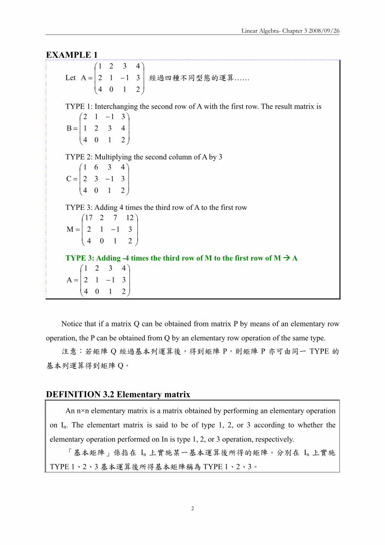
Linear Algebra- Chapter 3 20080926
2
EXAMPLE 1
Let ⎟⎟⎟
⎠
⎞
⎜⎜⎜
⎝
⎛minus=
210431124321
A 經過四種不同型態的運算helliphellip
TYPE 1 Interchanging the second row of A with the first row The result matrix is
⎟⎟⎟
⎠
⎞
⎜⎜⎜
⎝
⎛ minus=
210443213112
B
TYPE 2 Multiplying the second column of A by 3
⎟⎟⎟
⎠
⎞
⎜⎜⎜
⎝
⎛minus=
210431324361
C
TYPE 3 Adding 4 times the third row of A to the first row
⎟⎟⎟
⎠
⎞
⎜⎜⎜
⎝
⎛minus=
21043112
127217M
TYPE 3 Adding -4 times the third row of M to the first row of M A
⎟⎟⎟
⎠
⎞
⎜⎜⎜
⎝
⎛minus=
210431124321
A
Notice that if a matrix Q can be obtained from matrix P by means of an elementary row
operation the P can be obtained from Q by an elementary row operation of the same type
注意若矩陣 Q 經過基本列運算後得到矩陣 P則矩陣 P 亦可由同一 TYPE 的
基本列運算得到矩陣 Q
DEFINITION 32 Elementary matrix
An ntimesn elementary matrix is a matrix obtained by performing an elementary operation
on In The elementart matrix is said to be of type 1 2 or 3 according to whether the
elementary operation performed on In is type 1 2 or 3 operation respectively
「基本矩陣」係指在 In 上實施某一基本運算後所得的矩陣分別在 In 上實施
TYPE 123 基本運算後所得基本矩陣稱為 TYPE 123
Linear Algebra- Chapter 3 20080926
3
For example interchanging the first rows of I3 produces the elementary matrix
⎟⎟⎟
⎠
⎞
⎜⎜⎜
⎝
⎛=
100001010
E 為基本矩陣(Elementary matrix)係由 I3 的前二行互調或前兩列
互調取得
Note that E can be obtained by interchanging the first two columns of I3 In fact any
elementary matrix can be obtained in at least two ways ndash either by performing an elementary
row operation on In or by performing an elementary column operation on In Similarly
⎟⎟⎟
⎠
⎞
⎜⎜⎜
⎝
⎛ minus
100010201
也是基本矩陣(Elementary matrix)此矩陣可由兩種管道取得
is an elementary matrix since it can be obtained from I3 by an elementary column
operation of type 3 (adding -2 times the first column of I3 to the third column)
Theorem 31 Let AisinMmtimesn(F) and suppose that B is obtained from A by performing an elementary
row [column] operation Then there exists an mtimesm [ntimesn] elementary matrix E such that B
= EA [B = AE] IN fact E is obtained from Im [In] by performing the same elementary row
[column[ operation as that which was performed on A to obtain B Conversely if E is an
mtimesm [ntimesn] elementary matrix then EA [AE] is the matrix obtained from A by performing
the same elementary row [column] operation as that which produces E from Im [In]
令 AisinMmtimesn(F)並假設 B 是由 A 經實施某一基本列【或行】運算後所得到的矩
陣則存在一個 mtimesm 【或 ntimesn】基本矩陣 E使得 B = EA【或 B = AE】E 矩陣是
由 Im 【或 In】 經實施與「由 A 得到 B」相同的基本列【或行】運算後所得到的矩
陣反之若 E 是一個 mtimesm【或 ntimesn】的基本矩陣則 EA【或 AE】是由 A 經過與
「由 Im 【或 In】 得到 E」相同的基本列【或行】運算後所得到的矩陣
A Elementary row [column] operations B
Im Elementary row [column] operations E
B = EA [= AE]
Linear Algebra- Chapter 3 20080926
4
EXAMPLE 2 Consider the matrices A and B in Example 1 In this case B is obtained from A by
interchanging the second row of A with the first row Performing this same operation on I3
we obtain the elementary matrix
範例 1A 經過基本列運算(Interchanging the second row of A with the first
row) BIm 經過基本列運算(Interchanging the second row of A with the first
row) E則 B 亦可由 B = EA 取得
⎟⎟⎟
⎠
⎞
⎜⎜⎜
⎝
⎛=
100001010
E ⎟⎟⎟
⎠
⎞
⎜⎜⎜
⎝
⎛minus=
210431124321
A
⎟⎟⎟
⎠
⎞
⎜⎜⎜
⎝
⎛ minus==
210443213112
EAB
Consider the matrices A and C in Example 1 In this case C is obtained from A by
multiplying the second column of A by 3 Performing this same operation on I4 we obtain
the elementary matrix
範例 1A 經過基本行運算(Multiplying the second column of A by 3) C
In 經過基本行運算(Multiplying the second column of A by 3) E則 C 亦可由 C
= AE 取得
⎟⎟⎟⎟⎟
⎠
⎞
⎜⎜⎜⎜⎜
⎝
⎛
=
1000010000300001
E ⎟⎟⎟
⎠
⎞
⎜⎜⎜
⎝
⎛minus=
210431124321
A
C = AE = ⎟⎟⎟
⎠
⎞
⎜⎜⎜
⎝
⎛minus
210431324361
Theorem 32 Elementary matrices are invertible and the inverse of an elementary matrix is an
elementary matrix of the same type
基本矩陣為可逆矩陣且基本矩陣的反矩陣亦是同一型的基本矩陣
【Proof】
Let E be an elementary ntimesn matrix Then E can be obtained by an elementary row
Linear Algebra- Chapter 3 20080926
5
[column] operation on In By reversing the steps used to transform In into E we can
transform E back into In The result is that In can be obtained from E by an elementary row
[column] operation of the same type By Theorem 31 there is an elementary matrix E
such that nIEE = Therefore E is invertible and 1EE minus=
令 E 是 ntimesn 的基本矩陣E 可由 In 經實施一基本列或行運算取得若把用來實
施 In E 的運算對 E 實施亦可得到 In依據 Theorem 31 可知存在一基本矩陣E
使得 nIEE = 因此 E 為可逆且 1EE minus=
Elementary Matrices Elementary Matrices 1414
An elementary matrix is one that can be obtained from the identity matrix In through a single elementary row operation
⎥⎥⎥
⎦
⎤
⎢⎢⎢
⎣
⎡=
100010001
3I⎥⎥⎥
⎦
⎤
⎢⎢⎢
⎣
⎡=
010100001
1ER2 harr R3
⎥⎥⎥
⎦
⎤
⎢⎢⎢
⎣
⎡=
100050001
2E5R25R2
⎥⎥⎥
⎦
⎤
⎢⎢⎢
⎣
⎡=
100012001
3ER2+ 2R1R2+ 2R1
Operation TOperation T
Elementary Matrices Elementary Matrices 2424
⎥⎥⎥
⎦
⎤
⎢⎢⎢
⎣
⎡=
ihgfedcba
A
AEAfedihgcba
1
010100001
=sdot⎥⎥⎥
⎦
⎤
⎢⎢⎢
⎣
⎡=
⎥⎥⎥
⎦
⎤
⎢⎢⎢
⎣
⎡R2 harr R3
AEAihgfed
cba
2
100050001
555 =sdot⎥⎥⎥
⎦
⎤
⎢⎢⎢
⎣
⎡=
⎥⎥⎥
⎦
⎤
⎢⎢⎢
⎣
⎡5R2
AEAihg
cfbeadcba
3
100012001
222 =sdot⎥⎥⎥
⎦
⎤
⎢⎢⎢
⎣
⎡=
⎥⎥⎥
⎦
⎤
⎢⎢⎢
⎣
⎡+++
R2+ 2R1
Elementary Matrices Elementary Matrices 3434
Each elementary matrix is invertible
1221EI
RR +asymp
⎥⎥⎥
⎦
⎤
⎢⎢⎢
⎣
⎡=
100010021
1E
⎥⎥⎥
⎦
⎤
⎢⎢⎢
⎣
⎡=
100010001
I
IE 2R21R1 minus
asymprArr IEE =12 ie
22R21REI
minusasymp
⎥⎥⎥
⎦
⎤
⎢⎢⎢
⎣
⎡ minus=
100010021
E 1
Elementary Matrices Elementary Matrices 4444
If A and B are row equivalent matrices and A is invertible then B is invertibleSince A and B are row equivalent there exits a sequence of row operations T1hellipTn such that B=TnT1ALet the elementary matrices of these operations be E1hellipEn Thus B=En hellip E2 E1 AThe matrix A En hellipE2 E1 are all invertible
( )( )
1
n
1
3
1
2
1
111
11
1n
1
n
1
3
1
2
1
1
1
n
1
3
1
2
1
11
EEEEABBAEE
EEEAEEEEEA
minusminusminusminusminusminus
minusminus
minusminusminusminusminusminusminusminus
=rArr==
=
3-2 The Rank of a Matrix and Matrix Inverse
In this section we define the rank of a matrix We then use elementary operations to
compute the rank of a matrix and a linear transformation The section concludes with a
procedure for computing the inverse of an invertible matrix
何謂「矩陣的秩(Rank)」利用基本行列運算來計算矩陣與線性轉換的秩本節
還包括介紹如何計算可逆矩陣的反矩陣
Linear Algebra- Chapter 3 20080926
6
DEFINITION 33 Rank of a Matrix
If AisinMmtimesn(F) we define the rank of A denoted rank(A) to be the rank of the linear
transformation LA Fn Fm
若 AisinMmtimesn(F)則矩陣 A 的秩為線性轉換 LA Fn Fm的秩註記為 rank(A)
An ntimesn matrix is invertible if and only if its rank is n
一個 ntimesn 的矩陣為可逆的『若且唯若』條件為該矩陣的 Rank 為 n
Every matrix A is the matrix representation of the linear transformation LA with respect
to the appropriate standard ordered bases Thus the rank of the linear transformation LA is the
same as the rank of one of its matrix representation namely A
每一個矩陣 A 是線性轉換 LA 對於某個標準有序基底的矩陣表示式因此該線性轉
換 LA的 Rank 就等於矩陣表示式 A 的 Rank即 rank(LA) = rank(A)
DEFINITION 29
Let V and W be vector spaces and let T V W be linear If N(T) and R(T) are finite-
dimensional then we define the nullity of T denoted nullity(T) and the rank of T denoted
rank(T) to be the dimensions of N(T) and R(T) respectively
V 與 W 為向量空間且 T V W 為線性轉換
定義 T 的核次數(Nullity)nullity(T) = dimensions of N(T)
定義 T 的秩(Rank)rank(T) = dimension of R(T)
核次數(Nullity)與秩(Rank)分別代表 N(T)與 R(T)的維度
DEFINITION 211
Let β = u1 u2hellip un be an ordered basis for a finite-dimensional vectors space V
For xisinV let a1 a2hellip an be the unique scalars such that
令 β = u1 u2hellip un為有限向量空間 V 的有序基底則存在唯一的一組純量 a1
a2hellip an使得 V 內任意向量均可表達成該組基底的線性組合
sum=
=n
1iiiuax
we define the coordinate vector of x relative to β denoted β[x] by
Linear Algebra- Chapter 3 20080926
7
⎟⎟⎟⎟⎟
⎠
⎞
⎜⎜⎜⎜⎜
⎝
⎛
=β
n
2
1
a
aa
[x] 稱為 x 相對於有序基底 β的座標向量
DEFINITION 212
Suppose that V and W are finite-dimensional vector spaces with ordered bases β = v1
v2hellip vn and γ = w1 w2hellip wn respectively Let T V W be linear Then for each j 1
≦j≦n there exist unique scalars aijisinF 1≦i≦m such that
sum==
m
1iiijj wa)vT( for 1≦j≦n
We call the mtimesn matrix A defined by Aij = aij the matrix representation of T in the ordered bases β and γ and write γ
β= [T]A
If V = W and β = γ then we write β= [T]A
設 V 與 W 分別為有限維度的向量空間β = v1 v2hellip vn與 γ = w1 w2hellip
wn分別為 V 與 W 的有序基底且 T V W 為 V 映至 W 的線性轉換
對每一個 j(1≦ j≦n)而言存在唯一的純量 aij isinF(1≦ i≦m)使得
sum==
m
1iiijj wa)vT(
將 mtimesn 的矩陣 A 定義為 Aij = aij並稱呼 A 為線性轉換 T 的矩陣表達方式在
V 與 W 分別以 β 與 γ作為有序基底下A 可註記為 γβ= [T]A
若 V = W 且 β = γ則 β= [T]A
提示 sum==
m
1iiijj wa)vT( 為「將 vj的像 T(vj)表達成有序基底 γ的線性組合」
DEFINITION 217
Let A be an mtimesn matrix with entries from a field F We denote by LA the mapping LA
Fn Fm defined by LA(x) = Ax (the matrix product A and x) for each column vector xisinFn
We call LA a left-multiplication transformation
令 A 是 mtimesn 的矩陣所有元素均來自 FLA為 Fn映至 Fm的線性轉換並定義為
LA(x) = Ax其中 x 為行向量(Column vector)且 xisinFnLA被稱為左乘法轉換
Linear Algebra- Chapter 3 20080926
8
The next theorem extends this fact to any matrix representation of any linear
transformation defined on finite-dimensional vector spaces
Theorem 33 Let T V W be a linear transformation between finite dimensional vector spaces and
let β and γ be ordered bases for V and W respective Then rank(T) = rank( γβ[T] )
令 T V W且 β 與 γ 分別為有限維度向量空間 V 與 W 的有序基底則
rank(T) = rank( γβ[T] )
改寫 Definition 212
Suppose that Fn and Fm are finite-dimensional vector spaces with ordered bases β =
v1 v2hellip vn and γ = w1 w2hellip wn respectively Let LA Fn Fm be linear and defined
by LA(x) = Ax Then for each j 1≦j≦n there exist unique scalars aijisinF 1≦i≦m such
that sum=
=m
1iiijjA wa)v(L for 1≦j≦n We call the mtimesn matrix A defined by Aij = aij the matrix
representation of LA in the ordered bases β and γ and write γβ= ][LA A
Now that the problem of finding the rank of a linear transformation has been reduced to
the problem of finding the rank of a matrix we need a result that allows us to perform rank-
preserving operations on matrices The next theorem and its corollary tell us how to do this
線性轉換的 Rank 可以被簡化為找矩陣的 Rank如何找矩陣的 Rank
Theorem 34 Let A be an mtimesn matrix If P and Q are invertible mtimesm and ntimesn matrices respectively
then
令 A 為 mtimesn 的矩陣若 P 與 Q 分別為可逆的 mtimesm 與 ntimesn 矩陣則
(a) rank(AQ) = rank(A)
(b) rank(PA) = rank(A)
(c) rank(PAQ) = rank(A)
【Proof】
R(LAQ) = R(LALQ) = LALQ(Fn) = LA(LQ(Fn)) = LA(Fn) = R(LA)
Since LQ is onto rank(AQ) = dim(R(LAQ)) = dim(R(LA)) = rank(A)
Linear Algebra- Chapter 3 20080926
9
rank(PAQ) = rank(PA) = rank(A)
註Theorem 34 是為後續 Reduced Row Echelon Form of Matrix 做準備一個矩陣經過
基本行運算或基本列運算或基本行與列運算後並不會改變 RANK
Corollary
Elementary row and column operations on a matrix are rank-preserving
矩陣的基本列與行運算不會改變矩陣的 Rank
此推論結果是計算反矩陣解線性方程組的重要依據
Theorem 35 The rank of any matrix equals the maximum number of its linearly independent
columns that is the rank of a matrix is the dimension of the subspace generated by its
column
任一矩陣的 Rank 等於其最大線性獨立行向量數目即矩陣的 Rank 是由矩陣的
行向量生成的子空間的維度【LA Fn Fm】
【Proof】
For any AisinMmtimesn(F)
rank(A) = rank(LA) = dim(R(LA))
Let β be the standard basis of Fn Then β spans Fn and hence by Theorem 22
R(LA ) = span(LA (β)) = span(LA(e1) LA(e2)hellip LA(en))
But for any j we have seen in Theorem 213(b) that LA(ej) = Aej = aj where aj is the
jth column of A Hence R(LA ) = span(a1 a2 an)
Thus rank(A) = rank(LA) = dim(span(a1 a2 an))
對任意矩陣 Arank(A) = rank(LA) = dim(R(LA))
令 β為 Fn 的標準基底且生成 Fn
依據 Theorem 22
LA的值域 Range 可由 LA(β)來生成
R(LA) = span(LA (β)) = span(LA(e1) LA(e2)hellip LA(en))
對任意 j 而言由 Theorem 213(b) 可知 LA(ej) = Aej = aj其中aj 為 A 的第 j
個行(aj 相當於 Theorem 213(b)的 vj 或 Theorem 22 的 T(vj))因此 R(LA) =
Linear Algebra- Chapter 3 20080926
10
span(a1 a2 an)
所以 rank(A) = rank(LA) = dimension of R(LA) = dim(span(a1a2an))
Theorem 22 令 V 與 W 為向量空間且 T V W 為線性轉換若 β = v1 v2hellip vn
是定義域(Domain)V 的基底則 T 的值域 Range R(T)可由 T(β)來生成意即 R(T)
= span(T(β)) = span(T(v1) T(v2)hellip T(vn))
Theorem 213 A 為 mtimesn 的矩陣與 B 為 ntimesp 的矩陣uj 與 vj分別為 AB 與 B 的第 j 行
(1 j p≦ ≦ )則
(a) uj = A vj
(b) vj = B ej where ej is the jth standard vector of Fp
EXAMPLE 1
Let ⎟⎟⎟
⎠
⎞
⎜⎜⎜
⎝
⎛=
101110101
A
Observe that the first and second columns of A are linearly independent and that the
third column is a linear combination of the first two Thus
A 的第一行與第二行是線性獨立第三行則是前兩行的線性組合於是
rank(A) = dim⎟⎟⎟⎟
⎠
⎞
⎜⎜⎜⎜
⎝
⎛
⎟⎟⎟
⎠
⎞
⎜⎜⎜
⎝
⎛
⎪⎭
⎪⎬
⎫
⎟⎟⎟
⎠
⎞
⎜⎜⎜
⎝
⎛
⎪⎩
⎪⎨
⎧
⎟⎟⎟
⎠
⎞
⎜⎜⎜
⎝
⎛
⎟⎟⎟
⎠
⎞
⎜⎜⎜
⎝
⎛
111
010
101
span = 2
A 的第 1 行a1=⎟⎟⎟
⎠
⎞
⎜⎜⎜
⎝
⎛
101第 2 行a2=
⎟⎟⎟
⎠
⎞
⎜⎜⎜
⎝
⎛
010第 3 行a3=
⎟⎟⎟
⎠
⎞
⎜⎜⎜
⎝
⎛
111
In order to compute the rank of a matrix A it is frequently useful to postpone the use of
Theorem 35 until A has been suitable modified by means of appropriate elementary row and
column operations so that the number of linearly independent columns is obvious
為了利用 Theorem 35 求矩陣 A 的 Rank(等於最大線性獨立行向量數目)A 可
先經過基本列或行運算使其線性獨立的行數變得比較明顯
EXAMPLE 2 Let
Linear Algebra- Chapter 3 20080926
11
⎟⎟⎟
⎠
⎞
⎜⎜⎜
⎝
⎛=
211301121
A
If we subtract the first row of A from rows 2 and 3 (type 3 elementary row operations)
the result is
⎟⎟⎟
⎠
⎞
⎜⎜⎜
⎝
⎛
minusminus
110220121
If we now substract twice the first column from the second and substract the first
column from the third (type 3 elementary column operations) we obtain
⎟⎟⎟
⎠
⎞
⎜⎜⎜
⎝
⎛
minusminus
110220001
(後二行線性相依最大線性獨立行數為 2)
It is now obvious that the maximum number of linearly independent column of this matrix is 2 Hence the rank of A is 2
Theorem 36 Let A be an mtimesn matrix of rank r Then r m r n and by means of a finite number ≦ ≦
of elementary row and column operations A can be transformed into the matrix
D = ⎟⎟⎠
⎞⎜⎜⎝
⎛
32
1r
OOOI
where O1 O2 and O3 are zero matrices Thus Dii = 1 for i r and ≦
Dij = 0 otherwise
令 A 為 Rank 等於 r 的 mtimesn 矩陣則 r m≦ 且 r n≦ 經過有限次數的基本行與列
運算讓 A 化成 D = ⎟⎟⎠
⎞⎜⎜⎝
⎛
32
1r
OOOI
其中Ir 為對角元素為 1 的對角矩陣即 A 可經
過有限次數的基本行及列運算取得沿對角線前 r 個位置皆為 1其餘各處皆為 0 的
矩陣 D
【Proof】
If A is the zero matrix r = 0 In this case the conclusion follows with D = A
若 A 為零矩陣則 r = 0 且 D = A
Now suppose that AneO and r = rank(A) then r gt 0
The proof is by mathematical induction on m the number of rows of A
若 A 非零矩陣且 r = rank(A)則 r gt 0
Linear Algebra- Chapter 3 20080926
12
採用數學歸納法
Suppose that m = 1
A can be transformed into the matrix (1 0 hellip0)
So rank(D) = rank(A) = 1 by Corollary to Theorem 34 and Theorem 35 Thus the
theorem is established for m = 1
設 m = 1則 A 可以化成(1 0 hellip0)
依據 Corollary to Theorem 34 及 Theorem 35
rank(D) = rank(A) = 1
故本定理對 m = 1 的矩陣是成立的
Next assume that the theorem holds for any matrix with at most m - 1 row (for some m
gt1)
We must prove that the theorem holds for any matrix with m rows
其次假設本定理對至多含 m - 1 列的矩陣皆成立(m gt 1)
至於含 m 列的矩陣是否成立
If n = 1 Theorem 36 can be established in a manner analogous to that for m = 1
若 n = 1則可按 m = 1 的方式證明本定理對於 n = 1 的矩陣成立
We now suppose that n gt 1 Since A ne O Aijne0 for some i j By means of at most one
elementary row and at most one elementary column operation (each of type 1) We can
move the nonzero entry to the 11 position By means of of at most one additional type 2
operation we can assure a 1 in the 11 position By means of at most m ndash 1 type 3 row
operations and at most n ndash 1 type 3 column operations we can eliminate all nonzero entries
in the first row and the first column with the exception of the 1 in the 11 postion
Thus with a finite number of elementary operation A can be transformed into a
matrix
經過有限次數的基本行及列運算可將 A 轉換成
⎪⎪⎭
⎪⎪⎬
⎫
⎪⎪⎩
⎪⎪⎨
⎧
=
0B
0001
B where Brsquo is an (m-1)times(n-1) matrix
Brsquo has rank one less than B
Brsquo的 Rank 比 B 少 1
Since rank(A) = rank(B) = r rank(Brsquo) = r ndash 1 Therefore r ndash1 ≦ m ndash 1 and r ndash1 ≦
Linear Algebra- Chapter 3 20080926
13
n ndash 1 by the induction hypothesis Hence r ≦ m and r ≦ n
由於 rank(A) = rank(B) = r故 rank(Brsquo) = r ndash 1
依數學歸納法 r ndash1 ≦ m ndash 1 且 r ndash1 ≦ n ndash 1
因此 r ≦ m 且 r ≦ n
Also by the induction hypothesis Brsquo can be transformed by a finite number of
elementary row and column operations into the (m-1)times(n-1) matrix Drsquo such that
同樣地依據數學歸納法Brsquo 可經過有限次數的基本行與列運算轉換成 (m-
1)times(n-1) 的矩陣 Drsquo使得
Dlsquo= ⎟⎟⎠
⎞⎜⎜⎝
⎛ minus
65
41r
OOOI
where O4 O5 and O6 are zero matrices
That is Drsquo consists of all zeros except for its first r-1 diagonal entries which are ones
Let
⎪⎪⎭
⎪⎪⎬
⎫
⎪⎪⎩
⎪⎪⎨
⎧
=
0D
0001
D
We see that the theorem now follows once we show that D can be obtained from B by
means of a finite number of elementary row and column operations
D 可由 B 經過有限次基本行及列運算而取得
Thus since A can be transformed into B and B can be transformed into D each by a
finite number of elementary operations A can be transformed into D by a finite number of
elementary operations
經過有限次基本行及列運算A B D
Finally since Drsquo contains ones as its first r ndash 1 diagonal entries D contains ones as its
first r diagonal entries and zeros elsewhere
最後Drsquo沿對角線前 r-1 個位置皆為 1故 D 沿對角線前 r 個位置皆為 1其餘
各處皆為 0
EXAMPLE 3 Consider the maxtrix
⎟⎟⎟⎟⎟
⎠
⎞
⎜⎜⎜⎜⎜
⎝
⎛
=
192362100280844422420
A
Linear Algebra- Chapter 3 20080926
14
By means of a succession of elementary row and column operations we can transform
A into a matrix D as in Theorem 36
透過一系列的基本行與列運算將 A 轉換成 D
D
00000001000001000001
192362100280844422420
A =
⎟⎟⎟⎟⎟
⎠
⎞
⎜⎜⎜⎜⎜
⎝
⎛
==
⎟⎟⎟⎟⎟
⎠
⎞
⎜⎜⎜⎜⎜
⎝
⎛
=
By the corollary to Theorem 34 rank(A) = rank(D) Clearly however rank(D) = 3 so rank(A) = 3
Corollary 1 Let A be an mtimesn matrix of rank r Then there exist invertible matrices B and C of sizes
mtimesm and ntimesn respectively such that D = BAC where D = ⎟⎟⎠
⎞⎜⎜⎝
⎛
32
1r
OOOI
is the mtimesn matrix
in which O1 O2 and O3 are zero matrices
令 A 為 mtimesn 的矩陣Rank 為 r存在可逆的 mtimesm 矩陣 B 與 ntimesn 矩陣 C使得
D = BAC其中D = ⎟⎟⎠
⎞⎜⎜⎝
⎛
32
1r
OOOI
為 mtimesn 的矩陣O1O2 及 O3 為零矩陣
【Proof】
By Theorem 36 A can be transformed by means of a finite number of elementary
row and column operations into the matrix D
We can appeal to Theorem 31 each time we perform an elementary operation Thus
there exist elementary mtimesm matrices E1 E2hellipEp and elementary ntimesn matrices G1
G2hellipGq such that D = EpEp-1hellipE2E1AG1G2hellipGq
By Theorem 32 each Ej and Gj is invertible Let B = EpEp-1hellipE2E1 and C =
G1G2hellipGq Then B and C are invertible and D = BAC
依據 Theorem 36A 可經過有限次的基本列與行運算化成 D
引用 Theorem 31每一次皆實施某一個基本列運算於是存在基本的 mtimesm 矩
陣 E1 E2hellip Ep 與 基 本 的 ntimesn 矩 陣 G1 G2hellip Gq 使 得 D = EpEp-
1hellipE2E1AG1G2hellipGq
依據 Theorem 32 每一個基本矩陣 Ej與 Gj 皆為可逆令 B = EpEp-1hellipE2E1 與 C =
G1G2hellipGq於是 B 與 C 皆為可逆且 D = EpEp-1hellipE2E1AG1G2hellipGq = BAC
Linear Algebra- Chapter 3 20080926
15
Theorem 31 令 AisinMmtimesn(F)並假設 B 是由 A 經實施某一基本列【或行】運算後所得
到的矩陣則存在一個 mtimesm 【或 ntimesn】基本矩陣 E使得 B = EA【或 B = AE】E
矩陣是由 Im 【或 In】 經實施與「由 A 得到 B」相同的基本列【或行】運算後所得
到的矩陣反之若 E 是一個 mtimesm【或 ntimesn】的基本矩陣則 EA【或 AE】是由 A
經過與「由 Im 【或 In】 得到 E」相同的基本列【或行】運算後所得到的矩陣
Theorem 32 基本矩陣為可逆矩陣且基本矩陣的反矩陣亦是同一型的基本矩陣
Theorem 36 令 A 為 Rank 等於 r 的 mtimesn 矩陣則 r m≦ 且 r n≦ 經過有限次數的基
本行與列運算讓 A 化成 D = ⎟⎟⎠
⎞⎜⎜⎝
⎛
32
1r
OOOI
其中Ir為對角元素為 1 的對角矩陣
Corollary 2 Let A be an mtimesn matrix Then
(a) rank(At) = rank(A)
矩陣轉置後的 RANK 不變
(b) The rank of any matrix equals the maximum number of its linearly independent
rows that is the rank of a matrix is the dimension of the subspace generated by
rows
任一矩陣的 Rank 等於最大線性獨立列向量的數目即矩陣的 Rank 等於由該
矩陣列向量所生成的子空間的維度
(c) The rows and columns of any matrix generate subspaces of the same dimension
numerically equal to the rank of the matrix
任一矩陣的列向量與行向量生成的子空間的維度相同維度等於該矩陣的
Rank
【Proof】
By Corollary 1 there exist invertible matrices B and C such that D = BAC where D
satisfies the stated conditions of the corollary Taking transposes we have
Dt = (BAC) t = CtAtBt
Since B and C are invertible so are Bt and Ct
Hence by Theorem 34 rank(At) = rank(CtAtBt) = rank(Dt)
Suppose that r = rank(A)
Then Dt is an ntimesm matrix with the form of the matrix D in Corollary 1 and hence
Linear Algebra- Chapter 3 20080926
16
rank(Dt) = r by Theorem 35
Thus
rank(At) = rank(Dt) = r = rank(A)
依據 Corollary 1存在可逆矩陣 B 與 C使得 D = BAC
取其轉置可得Dt = (BAC) t = CtAtBt
由於 B 與 C 為可逆故 Bt 與 Ct 亦為可逆
依據 Theorem 34得知 rank(At) = rank(CtAtBt) = rank(Dt)
設 r = rank(A)
則 Dt為一 ntimesm 的矩陣型式與 D 相同(參考 Corollary 1)
且依據 Theorem 35 得知 rank(Dt) = r
於是 rank(At) = rank(Dt) = r = rank(A)
Theorem 34 Let A be an mtimesn matrix If P and Q are invertible mtimesm and ntimesn matrices
respectively then 令 A 為 mtimesn 的矩陣若 P 與 Q 分別為可逆的 mtimesm 與 ntimesn 矩陣
則
(a) rank(AQ) = rank(A)
(b) rank(PA) = rank(A)
(c) rank(PAQ) = rank(A)
Theorem 35 The rank of any matrix equals the maximum number of its linearly
independent columns that is the rank of a matrix is the dimension of the subspace
generated by its column 任一矩陣的 Rank 等於其最大線性獨立行向量數目即矩陣
的 Rank 是由矩陣的行向量生成的子空間的維度【LA Fn Fm】
Corollary 3 Every invertible matrix is a product of elementary matrices
每一可逆矩陣均可為基本矩陣的乘積
【Proof】
If A is an invertible ntimesn matrix then rank(A) = n Hence the matrix D in Corollary 1
equals In and there exist invertible matrices B and C such that In = BAC
As in the proof of Corollary 1 note that B = EpEp-1hellipE2E1 and C = G1G2hellipGq where
the Eirsquos and Girsquos are elementary matrices Thus A = B-1InC-1 = B-1C-1 so that
A = E1-1E2
-1hellipEp-1Gq
-1Gq-1-1hellipG1
-1
Linear Algebra- Chapter 3 20080926
17
The inverses of elementary matrices are elementary matrices however and hence A is
the product of elementary matrices
若 A 為可逆的 ntimesn 矩陣則 rank(A) = n
因此 Corollary 1 中的矩陣 D 為 In且存在可逆的 B 與 C 矩陣使得 In = BAC
如同 Corollary 1 的證明一樣B = EpEp-1hellipE2E1 且 C = G1G2hellipGq其中Eirsquos 與
Girsquos 皆為基本矩陣
於是A = B-1InC-1 = B-1C-1即 A = E1-1E2
-1hellipEp-1Gq
-1Gq-1-1hellipG1
-1
基本矩陣的反矩陣亦為基本矩陣A 是基本矩陣的乘積
Theorem 37 Let T V W and U W Z be linear transformations on finite-dimensional vector
spaces V W and Z and let A and B be matrices such that the product AB is defined Then
令 VW 與 Z 為有限維度的向量空間T V W 與 U W Z 為線性轉換且
A 與 B 為滿足乘積 AB 定義的矩陣則
(a) rank(UT) ≦ rank(U)
(b) rank(UT) ≦ rank(T)
(c) rank(AB) ≦ rank(A)
(d) rank(AB) ≦ rank(B)
【Proof】
(a) Clearly R(T)subeW
Hence R(UT) = UT(V) = U(R(T)) sube U(W) = R(U)
Thus rank(UT) = dim(R(UT)) ≦ dim (R(U)) = rank(U)
(c) By (a) rank(AB) = rank(LAB) = rank (LALB) ≦ rank(LA) = rank(A)
(d) By (c) and Corollary 2 to Theorem 36
rank(AB) = rank((AB)t) = rank(B t A t) ≦ rank(B t) = rank (B) (b) Let α β and γ be ordered bases for V W and Z respectively and let Arsquo = γ
β]U[
and Brsquo = βα]T[ Then ArsquoBrsquo = γ
α]UT[ by Theorem 211
Hence by Theorem 33 and (d)
rank(UT) = rank(ArsquoBrsquo) ≦ rank(Brsquo) = rank (T)
Theorem 211 Let V W and Z be finite-dimensional vector space with ordered bases α β
and γ respectively Let T V W and U W Z be linear transformation Then
Linear Algebra- Chapter 3 20080926
18
βα
γβ
γα = [T][U][UT] 令 VW 與 Z 是有限維度的向量空間αβ 與 γ 分別為 VW 與
Z 的有序基底令 T V W (先 α β) 且 U W Z (後 β γ)則 βα
γβ
γα = [T][U][UT]
Theorem 33 Let T V W be a linear transformation between finite dimensional vector
spaces and let β and γ be ordered bases for V and W respective Then rank(T) = rank( γ
β[T] ) 令 T V W且 β 與 γ 分別為有限維度向量空間 V 與 W 的有序基底
則 rank(T) = rank( γβ[T] )
EXAMPLE 4
(a) Let ⎟⎟⎠
⎞⎜⎜⎝
⎛minus
=11111121
A (第一列與第二列是 LI) rank(A) = 2
(b) Let ⎟⎟⎟
⎠
⎞
⎜⎜⎜
⎝
⎛=
003011011131
A (第三列與第一二列是 LD)rank(A) = 2
(c) Let ⎟⎟⎟
⎠
⎞
⎜⎜⎜
⎝
⎛
minus=
011111121321
A (三列為 LI) rank(A) = 3
The inverse of a Matrix
We have remarked that an ntimesn matrix is invertible if and only if its rank is n Since we
know how to compute the rank of any matrix we can always test a matrix to determine
whether it is invertible We now provide a simple technique for computing the inverse of a
matrix that utilizes elementary row operations
已知 ntimesn 矩陣為可逆的『若且唯若』條件為該矩陣的 Rank 等於 n
DEFINITION 34 Augmented Matrix Let A and B be mtimesn and mtimesp matrices respectively By the augmented matrix )BA(
we mean that the mtimes(n+p) matrix )BA( that is the matrix whose first n columns are the
columns of A and whose last p columns are the columns of B 設 A 與 B 分別為 mtimesn 與 mtimesp 的矩陣則增廣矩陣(Augmented matrix) )BA(
Linear Algebra- Chapter 3 20080926
19
為一 mtimes(n+p)的矩陣 )BA( 該矩陣的前 n 行(Column)為 A 的所有的行後 p
行為 B 的所有行
Let A be an invertible ntimesn matrix and consider the ntimes2n augmented matrix C= )IA( n
C= )IA( n )AI()IAAA(CA 1
nn111 minusminusminusminus ==
By Corollary 3 to Theorem 36 A-1 is the product of elementary matrices say
A = EpEp-1hellipE2E1 (A-1 是多個基本矩陣的乘積)
Thus )AI()IAAA(CA 1
nn111 minusminusminusminus == )AI(CA)IA(EEE 1
n1
n11ppminusminus
minus ==
We have the following result If A is an invertible invertible ntimesn matrix then it is
possible to transform the matrix (AIn) into the matrix (InA-1) by means of a finite
number of elementary row operations
若 A 為一可逆的 ntimesn 矩陣則可經過有限次數的基本列運算將矩陣 (AIn) 化成
(InA-1)
Conversely suppose that A is invertible and that for some ntimesn matrix B the matrix
(AIn) can be transformed into the matrix (InB) by a finite number of elementary row
operations Let E1 E2hellip Ep be the elementary matrices associated with these elementary row
operations as in Theorem 31 then
反之假設 A 是可逆且矩陣(AIn)可經有限次數的基本列運算轉換成矩陣(InB)
並令 E1 E2hellip Ep 分別為 Theorem 31 所稱的基本矩陣則
)BI()IA(EEE nn11pp =minus
Let M = EpEp-1hellipE2E1 we have 令 M = EpEp-1hellipE2E1
)BI()IA(EEE nn11pp =minus )BI()IA(M)MMA( nn ==
Linear Algebra- Chapter 3 20080926
20
Hence MA = In and M = B It follows that M = A-1 So B = A-1
可由 MA = In 及 M = B 得知M 就是 A-1故 B 就是 A-1
Thus we have the follow resultsIf A is an invertible ntimesn matrix and the matrix
(AIn) is transformed in a matrix of the form (InB) by means of a finite number of
elementary row operations then B=A-1
若 A 為一可逆的 ntimesn 矩陣且矩陣 (AIn) 可經有限次數的基本列運算化成
(InB)則 B=A-1
If on the other hand A is an ntimesn matrix that is not invertible then rank(A) lt n Hence
any attempt to transform (AIn) into a matrix of the form (InB) by means of elementary row
operations must fail
反之若 A 是一不可逆的 ntimesn 矩陣則 rank(A) lt n因此任何想利用基本列運算
要將矩陣 (AIn) 化成 (InB)的努力必定失敗
Thus we have the follow results If A is an notinvertible ntimesn matrix then any attempt
to transform (AIn) into a matrix of the form (InB) produce a row whose first n entries
are zeros
若 A 是一不可逆的 ntimesn 矩陣任何想將矩陣 (AIn) 化成 (InB)的努力最後會
產生一前 n 個元素均為 0 的列
EXAMPLE 5
We determine whether the matrix ⎟⎟⎟
⎠
⎞
⎜⎜⎜
⎝
⎛=
133242420
A is invertible and if it is we
compute its inverse
A 是否為可逆矩陣
We attempt to use elementary row operations to transfer
Linear Algebra- Chapter 3 20080926
21
⎟⎟⎟
⎠
⎞
⎜⎜⎜
⎝
⎛=
100010001
133242420
)IA( into a matrix of the form (InB)
看看能否利用基本行與列運算將矩陣 (AIn) 化成 (InB)
Interchanging rows 1 and 2
⎟⎟⎟
⎠
⎞
⎜⎜⎜
⎝
⎛
100001010
133420242
Multiplying the first row by 12
⎟⎟⎟
⎠
⎞
⎜⎜⎜
⎝
⎛
10000100
133420121 2
1
Adding -3 times row 1 to row 3
⎟⎟⎟
⎠
⎞
⎜⎜⎜
⎝
⎛
minusminusminus 1000100
230420121
23
21
Multiplying row 2 by 12 to obtain 1 in the 22 position
⎟⎟⎟
⎠
⎞
⎜⎜⎜
⎝
⎛
minus
minus
minusminus 100000
230210121
23
21
21
Adding -2 times row 2 to row 1 and 3 times row 2 to row 3
⎟⎟⎟
⎠
⎞
⎜⎜⎜
⎝
⎛
minus
minusminus
10001
400210301
23
2321
21
Multiplying row 3 by 14
⎟⎟⎟
⎠
⎞
⎜⎜⎜
⎝
⎛
minus
minusminus
41
83
8321
21
0001
100210301
Adding appropriate multiply of row 3 to row 1 and 2 completes the process
⎟⎟⎟
⎠
⎞
⎜⎜⎜
⎝
⎛
minusminus
minus
41
83
83
21
43
41
43
85
81
100010001
目標達成
Thus A is invertible and ⎟⎟⎟
⎠
⎞
⎜⎜⎜
⎝
⎛
+minus+minus+minus+minus+
=minus
41
83
83
21
43
41
43
85
81
1A
Linear Algebra- Chapter 3 20080926
22
EXAMPLE 6
We determine whether the matrix ⎟⎟⎟
⎠
⎞
⎜⎜⎜
⎝
⎛minus=451112
121A is invertible and if it is we
compute its inverse
A 是否為可逆矩陣
We attempt to use elementary row operations to transfer
⎟⎟⎟
⎠
⎞
⎜⎜⎜
⎝
⎛minus=
100010001
451112
121)IA( into a matrix of the form (InB)
看看能否利用基本行與列運算將矩陣 (AIn) 化成 (InB)
Adding -2 times row 1 to row 2 and -1 times row 1 to row 3 then addig row 2 to row
3
⎟⎟⎟
⎠
⎞
⎜⎜⎜
⎝
⎛minus
100010001
451112
121
⎟⎟⎟
⎠
⎞
⎜⎜⎜
⎝
⎛
minusminusminusminus
101012001
330330
121
⎟⎟⎟
⎠
⎞
⎜⎜⎜
⎝
⎛
minusminusminusminus
113012001
000330
121
is a matrix with row whose first 3 entries are zeros Therefore A is not invertible
最後一列前 3 個元素均為 0
EXAMPLE 7 Let T P2(R) P2(R) be defined by T(f(x)) = f(x)+frsquo(x)+frdquo(x) where frsquo(x) and frdquo(x)
denote the first and second derivatives of f(x) We use Corollary 1 to Theorem 218 to test
T for invertibility and compute the inverse if T is invertible Taking β=1 x x2 to be the
standard ordered basis of P2(R) we have
令 T P2(R) P2(R) 為線性轉換且定義為 T(f(x)) = f(x)+frsquo(x)+frdquo(x)利用
Corollary 1 to Theorem 218 來測試 T 是否可逆並計算其逆轉換取 β=1 x x2為
P2(R)的標準有序基底
T(1) = 1 = 1bull1+0bullx+0bullx2
T(x) = 1+x = 1bull1+1bullx+0bullx2
Linear Algebra- Chapter 3 20080926
23
T(x2) = 2+2x+x2 = 2bull1+2bullx+1bullx2
⎟⎟⎟
⎠
⎞
⎜⎜⎜
⎝
⎛=β
100210211
[T] 稱為 T 相對有序基底 β的座標向量
依據 Corollary 1 to Theorem 218 T 可逆『若且唯若』 β[T] 可逆且
1-1 )[T](][T minusββ =
Using the method of Examples 5 and 6 we can show that β[T] is invertible with
inverse
⎟⎟⎟
⎠
⎞
⎜⎜⎜
⎝
⎛minus
minus=minus
β
100210
011)([T] 1
Thus T is is invertible and βminusminus
β = ][T)([T] 11 Hence by Theorem 214 we have
⎟⎟⎟
⎠
⎞
⎜⎜⎜
⎝
⎛minusminus
=⎟⎟⎟
⎠
⎞
⎜⎜⎜
⎝
⎛
⎟⎟⎟
⎠
⎞
⎜⎜⎜
⎝
⎛minus
minus=++ β
minus
2
21
10
2
1
02
2101
aa2aaa
aaa
100210
011)]xaxa(a[T
Therefore T-1(a0+a1x+a2x2) = (a0-a1)+(a1-2a2)x+a2x2 Corollary 1 to Theorem 218 Let V be finite-dimensional vector space with an ordered basis β and let T V V be linear Then T is invertible if and only if β[T] is invertible
Furthermore 1-1 )[T](][T minusββ = V 為有限維度的向量空間β 是 V 的有序基底令 T
V V 為線性轉換 T 為可逆的『若且唯若』條件為 β[T] 可逆再者
1-1 )[T](][T minusββ =
Theorem 214 Let V and W be finite-dimensional vector spaces having ordered bases β and γ respectively and let T V W be linear Then for each uisinV we have β
γβγ = [u][T][T(u)]
V 與 W 為有限維度的向量空間β 與 γ分別 V 與 W 的有序基底令 T V W 為線
性轉換則 V 中的 u 映至 W 的結果 T(u) 相對於有序基底 γ 的座標向量為
βγβγ = [u][T][T(u)]
Invertible and Inverse of MATRIX Let A be an n times n matrix If a matrix B can be found such that AB = BA = In then A is
Linear Algebra- Chapter 3 20080926
24
said to be invertible and B is called the inverse of A (denote B = A-1 and A-k=(A-1)k )
If such a matrix B does not exist then A has no inverse
EXAMPLE
⎥⎦
⎤⎢⎣
⎡=
4321
A and ⎥⎦
⎤⎢⎣
⎡minus
minus=
21
23
12B
221
23
221
23
I1001
432112
BA
I100112
4321
AB
=⎥⎦
⎤⎢⎣
⎡=⎥
⎦
⎤⎢⎣
⎡⎥⎦
⎤⎢⎣
⎡minus
minus=
=⎥⎦
⎤⎢⎣
⎡=⎥
⎦
⎤⎢⎣
⎡minus
minus⎥⎦
⎤⎢⎣
⎡=
Thus AB = BA = I2 proving that the matrix A has inverse B
Theorem The inverse of an invertible matrix is unique
Let B and C be inverse of A
Thus AB = BA = In and AC = CA = In
Multiply both sides of the equation AB = In by C
C(AB) = CIn (CA)B = C
InB = C B = C
Thus an invertible matrix has only one inverse
How to find AHow to find A--11
Based on the GaussBased on the Gauss--Jordan algorithmJordan algorithmLet A be an invertible matrix Then AALet A be an invertible matrix Then AA--11=I=Inn
Let the columns of Let the columns of AA--11 be be XX11 XX22 helliphellip XXnn and the columns of I and the columns of Inn be be CC11CC22helliphellipCCnn
Find AFind A--11 by finding by finding XX11 XX22 helliphellip XXnn Write the equation AAWrite the equation AA--11=I=Inn in the formin the form
[ ] [ ]n21nn211 CCCI XXXALet LL ==minus
[ ] [ ][ ] [ ]n21n21
n21n21
CCCAXAXXACCCXXXALL
LL
=rArr=
nn2211 CAXCAX CAX === LThus
How to find AHow to find A--11
Solving these systems by using Gauss-Jordan elimination on the large augmented matrix [AC1 C2hellipCn]
Thus when A-1 exits
[ ] [ ] [ ] 1n
1nn ABwhereBIAIIA minusminus ==asympasympL
If the reduced echelon form of [If the reduced echelon form of [AIAInn] is computed and ] is computed and the first part is not of the form Ithe first part is not of the form Inn then A has no inversethen A has no inverse
[ ][ ]n21n
n21
XXXI CCCAmatrix augmented
LL
L
asympasymp
Linear Algebra- Chapter 3 20080926
25
Example Example 1212
⎥⎥⎥
⎦
⎤
⎢⎢⎢
⎣
⎡
minusminusminusminusminus
=100531010532001211
]IA[ 3
⎥⎥⎦
⎤
⎢⎢⎣
⎡minusminusminus
minusminus
+minus+
asymp
101320012110001211
1RR1R3
2)(R2
⎥⎥⎦
⎤
⎢⎢⎣
⎡minus
minusminusminusasymp
101320012110001211
R2)1(
⎥⎥⎥
⎦
⎤
⎢⎢⎢
⎣
⎡
minusminusminusminusminus
=531532211
ADetermine the inverse of
Example Example 2222
⎥⎥⎦
⎤
⎢⎢⎣
⎡
minusminusminusminus
minus++asymp
123100012110013101
R2)2(R3R2R1
⎥⎥⎦
⎤
⎢⎢⎣
⎡
minusminusminus
minus++asymp
123100135010010001
R3)1(R2R3R1
123135110
A 1
⎥⎥⎥
⎦
⎤
⎢⎢⎢
⎣
⎡
minusminusminus=minus
⎥⎥⎦
⎤
⎢⎢⎣
⎡
minusminus
minus
+minus+asymp
135000011210012301
3R2R3R2)1(R1
ExampleExampleDetermine the inverse of
⎥⎥⎦
⎤
⎢⎢⎣
⎡
minus=
412721511
A
⎥⎥⎦
⎤
⎢⎢⎣
⎡
minus=
100412010721001511
][ 3IA
⎥⎥⎦
⎤
⎢⎢⎣
⎡
minusminusminusminus
minus+minus+asymp
102630011210001511
R1)2(R31)R1(R2
There is no need to proceed further There is no need to proceed further The reduced echelon form cannot have a one in the (3 3) locatioThe reduced echelon form cannot have a one in the (3 3) location n
The reduced echelon form cannot be of the form [IThe reduced echelon form cannot be of the form [Inn B] B] Thus Thus AAndashndash11 does not existdoes not exist
Properties of Matrix InverseProperties of Matrix Inverse
Let Let AA and and BB be invertible matrices andbe invertible matrices and cc a nonzero scalar a nonzero scalar ThenThen
AA =minusminus 11)( 111 1)( 2 minusminus = A
ccA
111)( 3 minusminusminus = ABAB
nn AA )()( 4 11 minusminus =tt AA )()( 5 11 minusminus =
Color Models Color Models 1212
A color model in the context of graphics is a method of A color model in the context of graphics is a method of implementing colorsimplementing colorsThe common used models include RGB model and YIQ modelThe common used models include RGB model and YIQ modelThe RGB model is used in computer monitors and the YIQ model The RGB model is used in computer monitors and the YIQ model is used in television screensis used in television screensAn RGB computer signal can be converted to a YIQ television An RGB computer signal can be converted to a YIQ television signal using the matrix transformationsignal using the matrix transformation
⎥⎥⎥
⎦
⎤
⎢⎢⎢
⎣
⎡
⎥⎥⎥
⎦
⎤
⎢⎢⎢
⎣
⎡
minusminusminus=
⎥⎥⎥
⎦
⎤
⎢⎢⎢
⎣
⎡
BGR
311523212321275596
114587299
QIY
YIQgtRGBYIQgtRGB
Color Models Color Models 2222
A signal is converted from a television screen to a computer monA signal is converted from a television screen to a computer monitor itor using inverse of the above matrixusing inverse of the above matrix
⎥⎥⎥
⎦
⎤
⎢⎢⎢
⎣
⎡
⎥⎥⎥
⎦
⎤
⎢⎢⎢
⎣
⎡
minusminusminus=
⎥⎥⎥
⎦
⎤
⎢⎢⎢
⎣
⎡rArr
⎥⎥⎥
⎦
⎤
⎢⎢⎢
⎣
⎡
⎥⎥⎥
⎦
⎤
⎢⎢⎢
⎣
⎡
minusminusminus=
⎥⎥⎥
⎦
⎤
⎢⎢⎢
⎣
⎡minus
QIY
0751108116472721
6209561
BGR
QIY
311523212321275596
114587299
BGR 1
CryptographyCryptography 密碼學密碼學 1212
Cryptography is the process of coding and decoding messagesCryptography is the process of coding and decoding messagesThe technique can be traced back to the ancient Greeks Today The technique can be traced back to the ancient Greeks Today governments use sophisticated methods of coding and decoding governments use sophisticated methods of coding and decoding messagesmessagesOne type of code that is extremely difficult to break makes use One type of code that is extremely difficult to break makes use of a of a large matrix to encode a message large matrix to encode a message The receiver of the message decodes it using the inverse of the The receiver of the message decodes it using the inverse of the matrixmatrixThe first matrix is called the encoding matrix and its inverse The first matrix is called the encoding matrix and its inverse is is called the decoding matrixcalled the decoding matrix
Cryptography Cryptography 密碼學密碼學 2222
A A-1Message
Encoding MatrixEncoding Matrix
Decoded MessageTransmission
Decoding MatrixDecoding Matrix
Linear Algebra- Chapter 3 20080926
26
Example Example 1212
Let the message be Let the message be BUY IBM STOCKBUY IBM STOCKAnd the encoding matrix beAnd the encoding matrix be
⎥⎥⎥
⎦
⎤
⎢⎢⎢
⎣
⎡ minusminusminus
434110433
B U Y B U Y -- I B M I B M -- S T O C KS T O C K2 21 25 27 9 2 13 27 19 20 15 3 112 21 25 27 9 2 13 27 19 20 15 3 11
⎥⎥⎥
⎦
⎤
⎢⎢⎢
⎣
⎡ minusminusminusminusminus=
⎥⎥⎥
⎦
⎤
⎢⎢⎢
⎣
⎡
⎥⎥⎥
⎦
⎤
⎢⎢⎢
⎣
⎡ minusminusminus
2331372091431715418461146
222117196116169
27319225271527921112013272
434110433
EncodingEncoding
Example Example 2222
Let the message be Let the message be BUY IBM STOCKBUY IBM STOCKAnd the decoding matrix beAnd the decoding matrix be
⎥⎥⎥
⎦
⎤
⎢⎢⎢
⎣
⎡
minusminus 334344101
B U Y B U Y -- I B M I B M -- S T O C KS T O C K2 21 25 27 9 2 13 27 19 20 15 3 112 21 25 27 9 2 13 27 19 20 15 3 11
⎥⎥⎥
⎦
⎤
⎢⎢⎢
⎣
⎡=
⎥⎥⎥
⎦
⎤
⎢⎢⎢
⎣
⎡ minusminusminusminusminus
⎥⎥⎥
⎦
⎤
⎢⎢⎢
⎣
⎡
minusminus 27319225271527921112013272
2331372091431715418461146
222117196116169
334344101
DecodingDecoding
3-3 Systems of Linear Equations ndash Theoretical Aspects
The system of equations
mnmn22m11m
2nn2222121
1nn1212111
bxaxaxa
bxaxaxabxaxaxa
=+++
=+++=+++
(S)
were aij and bi (1≦i≦m and 1≦j≦n) are scalars in a field F and x1 x2hellipxn are n
variables taking values in F is called a system of m linear equations in n unknows over the
field F
上式稱為佈於 Field F 含有 n 個未知數m 個線性方程式的系統或方程組(system
of m linear equations in n unknows)
The mtimesn matrix
⎟⎟⎟⎟⎟
⎠
⎞
⎜⎜⎜⎜⎜
⎝
⎛
=
mn2m1m
n22221
n11211
aaa
aaaaaa
A is called the coefficient matrix of the
system (S)(係數矩陣) If we let
⎟⎟⎟⎟⎟
⎠
⎞
⎜⎜⎜⎜⎜
⎝
⎛
=
n
2
1
x
xx
x and
⎟⎟⎟⎟⎟
⎠
⎞
⎜⎜⎜⎜⎜
⎝
⎛
=
m
2
1
b
bb
b Then the system (S) may
be rewritten as a single matrix equation Ax = b(單一矩陣方程式)
To exploit the results that we have developed we often consider a system of linear
equations as a single matrix equation
Linear Algebra- Chapter 3 20080926
27
A solution to the system (S) is an n-tuple n
n
2
1
F
s
ss
s isin
⎟⎟⎟⎟⎟
⎠
⎞
⎜⎜⎜⎜⎜
⎝
⎛
= such that As = b The set of
all solutions to the system (S) is called the solution set of the system(解集合) System (S)
is called consistent(相容) if its solution set is nonempty otherwise it is called
inconsistent(不相容)
方程組(S)的解為一 n 序組該序組可以使 As = b方程組的所有解所成的集合
稱為該方程組的解集合(Solution set)方程組的解集合非空集合者稱為「相容」解
集合空集合者稱為「不相容」
EXAMPLE 1
Consider 6x2xx1xx3x2
321
321
=+minus=++
that is ⎟⎟⎠
⎞⎜⎜⎝
⎛=
⎟⎟⎟
⎠
⎞
⎜⎜⎜
⎝
⎛
⎟⎟⎠
⎞⎜⎜⎝
⎛minus 6
1
xxx
211132
3
2
1
(以矩陣表示)
This system has many solutions such as ⎟⎟⎟
⎠
⎞
⎜⎜⎜
⎝
⎛minus=
726
s and ⎟⎟⎟
⎠
⎞
⎜⎜⎜
⎝
⎛
minusminus=
34
8s
Consider 1xx0xx
21
21
=+=+
that is ⎟⎟⎠
⎞⎜⎜⎝
⎛=⎟⎟
⎠
⎞⎜⎜⎝
⎛⎥⎦
⎤⎢⎣
⎡10
xx
1111
2
1
顯然地方程組無解
We begin our study of system of linear equations by examining the class of
homogeneous system of linear equations 先討論齊次方程組
DEFINITION 35 Homogeneous amp Nonhomogeneous
A system Ax=b of m linear equations in n unknowns is said to be homogeneous if b=0
Otherwise the system is said to be nonhomogeneous
方程組 Ax = bb = 0 稱為齊次方程組否則稱為非齊次方程組
Any homogeneous system has at least one solution namely the zero vector The next
result gives further information about the set of solutions to a homogeneous system
Linear Algebra- Chapter 3 20080926
28
齊次方程組至少有一個解那就是『零向量』
Theorem 38 Let Ax = 0 be a homogeneous system of m linear equations in n unknowns over a field
F Let K denote the set of all solutions to Ax = 0 Then K = N(LA) hence K is a subspace
of Fn of dimension n - rank(LA) = n- rank(A)
令 Ax = 0 代表一佈於 Field 含有 n 個未知數m 個線性方程式的方程組若令
K 代表該方程組的解集合(Solution set)則 K = N(LA)K 為 Fn 內的子空間且其維
度為 n ndash rank (LA) = n - rank(A)
【Proof】
Clearly K = sisinFn As = 0 = N(LA) The second part now follows from the
dimension theorem
Nullity(T)+rank(T) = dim(V)
Nullity (LA) = dim (Fn) ndashrank (LA ) = n ndash rank (A)
DEFINTION 27 Let V and W be vector space and let T V W be linear We define
the null space (or kernel) N(T) of T to be the set of all vectors x in V such that T(x) = 0
that is N(T) = xisinV T(x) = 0 V 與 W 為向量空間且 T V W 為線性轉換定義
線性轉換 T 的 Null space 為 V 內所有滿足 T(x) = 0 的向量 x 所形成的集合註記為
N(T)Null space 的元素 x 經線性轉換 T 轉換後所對應的「像」為 0意即 T(x) = 0
Null space 內的元素的「像」皆為 0
DEFINITION 217 Let A be an mtimesn matrix with entries from a field F We denote by LA
the mapping LA Fn Fm defined by LA(x) = Ax (the matrix product A and x) for each
column vector xisinFn We call LA a left-multiplication transformation 令 A 是 mtimesn
的矩陣所有元素均來自 FLA 為 Fn 映至 Fm的線性轉換並定義為 LA(x) = Ax其中
x 為行向量(Column vector)且 xisinFnLA被稱為左乘法轉換
Theorem 23 (Dimension Theorem) Let V and W be vector spaces and let T V W be
linear If V is finite-dimensional then Nullity(T) + rank(T) = dim(V) T 的核次數
(Nullity)與秩(Rank)的和等於定義域的維度 dim(V)
Corollary Let Ax = 0 be a homogeneous system of m linear equations in n unknowns over a field
Linear Algebra- Chapter 3 20080926
29
F If m lt n the system Ax = 0 has a nonzero solution
令 Ax = 0 代表一佈於 Field 含有 n 個未知數m 個線性方程式的方程組若 m
lt n則該方程組具有一非零解
【Proof】
Suppose that m lt n Then rank(A) = rank (LA)≦m Hence dim(K) = n - rank(LA) ≧
n ndash m gt 0 where K = N(LA) Since dim(K) gt 0 Kne 0 Thus there exists a nonzero
vector sisinK so s is a nonzero solution to Ax = 0
設 m lt n則 rank(A) = rank (LA) ≦ m依據 Theorem 38K = sisinFn As = 0
= N(LA) = dim(K) = n - rank(LA) ≧ n ndash m gt 0表示 dim(K) gt 0Kne 0故存在非
零向量 s使得 Ax = 0
EXAMPLE 2
Consider 0xxx
0xx2x
321
321
=minusminus=++
Let ⎟⎟⎠
⎞⎜⎜⎝
⎛minusminus
=111
121A be the coefficient matrix of this system It is clear that rank(A)
= 2 If K is the solution set of this system then dim(K) = 3-2 = 1 Thus any nonzero
solution constitutes a basis for K
若 K 是方程組的解所組成的集合(簡稱為解集合)依 Theorem 38 得知 dim(K)
= 3 - 2 = 1因此任一非零解將形成 K 的基底
For example since ⎟⎟⎟
⎠
⎞
⎜⎜⎜
⎝
⎛minus32
1 is a solution to the given system
⎪⎭
⎪⎬
⎫
⎪⎩
⎪⎨
⎧
⎟⎟⎟
⎠
⎞
⎜⎜⎜
⎝
⎛minus32
1 is a basis for
K Thus any vector in K is of the form ⎟⎟⎟
⎠
⎞
⎜⎜⎜
⎝
⎛minus=
⎟⎟⎟
⎠
⎞
⎜⎜⎜
⎝
⎛minus
t3t2
t
32
1t where tisinR
例如因⎟⎟⎟
⎠
⎞
⎜⎜⎜
⎝
⎛minus32
1是方程組的一個解故
⎪⎭
⎪⎬
⎫
⎪⎩
⎪⎨
⎧
⎟⎟⎟
⎠
⎞
⎜⎜⎜
⎝
⎛minus32
1 為 K 的基底K 內的任一向量均
具有如下形式
⎟⎟⎟
⎠
⎞
⎜⎜⎜
⎝
⎛minus=
⎟⎟⎟
⎠
⎞
⎜⎜⎜
⎝
⎛minus
t3t2
t
32
1t
Linear Algebra- Chapter 3 20080926
30
We now turn to the study of nonhomogeneous systems Our next result shows that the
solution set of a nonhomogeneous system Ax = b can be described in terms of the solution of
the homogeneous system Ax = 0 We refer to the equation Ax = 0 as the homogeneous system
corresponding to Ax = b
以下將進一步探討「非齊次方程組」非齊次方程組 Ax = b 的解集合可利用齊次方
程組 Ax = 0 的解來加以說明因此我們可將 Ax = 0 視為 Ax = b 的齊次方程組
Theorem 39 Let K be the solution set of a system of linear equations Ax = b and let KH be the
solution set of the corresponding homogeneous system Ax = 0 Then for any solution s to
Ax = b K =s + KH = s+k kisinKH
設 K 為線性方程組 Ax = b 的解集合且 KH為對應的齊次方程組的解集合則
對 Ax = b 的任一個解 s 而言K =s + KH = s+k kisinKH
【Proof】
Let s be any solution to Ax = b
We must show that K =s + KH
If wisinK then Aw = b Hence
A(w - s) = Aw ndash As = b ndash b = 0
So w - sisinKH
Thus there exists kisinKH such that w - s = k
It follows that w = s + k isin s +KH and therefore Ksube s +KH
Conversely suppose that wisins +KH then w = s + k for some kisinKH
But then Aw = A(s + k) = As + Ak = b + 0 = b so wisinK
Therefore s +KHsubeK and thus K=s +KH
令 s 為 Ax = b 的任一個解我們必須證明「K =s + KH」
若 wisinK則 Aw = b(即 w 為 Ax = b 的解)
於是 A(w - s) = Aw ndash As = b ndash b = 0
所以 w - sisinKH(即 w-s 為 Ax = 0 的解)
w - s 既然是 KH的元素表示有一元素 kisinKH使得 w - s = kw = s + k
w = s + kisins +KH
Linear Algebra- Chapter 3 20080926
31
因此 Ksube s +KH
反之假設 wisins +KH則 KH中存在一元素 k(kisinKH)使得 w = s + k
因 Aw = A(s + k) = As + Ak = b + 0 = b
故 wisinK 是 Ax = b 的解
因此s +KHsubeK
總結K=s +KH
EXAMPLE 3
Consider 4xxx7xx2x
321
321
minus=minusminus=++
The corresponding homogeneous system is the system in Example 2 It is easily
verified that ⎟⎟⎟
⎠
⎞
⎜⎜⎜
⎝
⎛=
411
s is a solution to the preceeding nonhomogeneous system So the
solution set of the system is ⎪⎭
⎪⎬
⎫
⎪⎩
⎪⎨
⎧isin
⎟⎟⎟
⎠
⎞
⎜⎜⎜
⎝
⎛minus+
⎟⎟⎟
⎠
⎞
⎜⎜⎜
⎝
⎛= Rt
32
1t
411
K by Theorem 39
⎟⎟⎟
⎠
⎞
⎜⎜⎜
⎝
⎛=
411
s 是非齊次方程組 Ax = b 的解
⎟⎟⎟
⎠
⎞
⎜⎜⎜
⎝
⎛minus32
1是齊次方程組的解
依據 Theorem 39 得知線性方程組 Ax = b 的解集合⎪⎭
⎪⎬
⎫
⎪⎩
⎪⎨
⎧isin
⎟⎟⎟
⎠
⎞
⎜⎜⎜
⎝
⎛minus+
⎟⎟⎟
⎠
⎞
⎜⎜⎜
⎝
⎛= Rt
32
1t
411
K
The following theorem will provide us with a means of computing solutions to certain
system of linear equations
Theorem 310~311 提供計算線性方程組的解的方法
Theorem 310 Let Ax = b be a system of n linear equations in n unknowns If A is invertible then the
Linear Algebra- Chapter 3 20080926
32
system has exactly one solution namely A-1b Conversely if the system has exactly one
solution then A is invertible
令 Ax = b 為含 n 個未知數n 個線性方程式的方程組若 A 為可逆則方程組
恰有一個解解為 A-1b反之若該方程組恰有一個解則 A 為可逆
【Proof】
Suppose that A is invertible
Substituting A-1b into system we have A(A-1b)=( AA-1)b = b
Thus A-1b is a solution
If s is an arbitrary solution then As = b
Multiplying both sides by A-1 gives s= A-1b
Thus the system has one and only one solution namely A-1b
假設 A 為可逆將 A-1b 代入方程組可得 A(A-1b)=( AA-1)b = b
故 A-1b 確為方程組的解
若 s 為方程組的任意解則 As = b
兩邊乘上 A-1可得 s= A-1b
因此方程組僅有唯一的解 A-1b
Conversely suppose that the system has exactly one solution s
Let KH denot the solution set for the corresponding homogeneous system Ax = 0
By Theorem 39 s = s + KH But it is so only if KH = 0 Thus N(LA) = 0 and
hence A is invertible
反之假設方程組恰有一個解 s
令 KH為相對應齊次方程組 Ax = 0 的解集合
依據 Theorem 39要能s = s + KH唯有 KH = 0
KH = 0即表示 N(LA) = 0故 A 為可逆
EXAMPLE 4 Consider the following system of three linear equations in three unknowns
1xx3x33x2x4x2
2x4x2
321
321
32
=++=++
=+
In Example 5 of Section 32 we compute the inverse of the coefficient matrix A of
this system Thus the system has exactly one solution namely
Linear Algebra- Chapter 3 20080926
33
⎟⎟⎟
⎠
⎞
⎜⎜⎜
⎝
⎛=
133242420
A⎟⎟⎟
⎠
⎞
⎜⎜⎜
⎝
⎛
+minus+minus+minus+minus+
=minus
41
83
83
21
43
41
43
85
81
1A
⎟⎟⎟
⎠
⎞
⎜⎜⎜
⎝
⎛
minus+minus
=⎟⎟⎟
⎠
⎞
⎜⎜⎜
⎝
⎛
⎟⎟⎟
⎠
⎞
⎜⎜⎜
⎝
⎛
+minus+minus+minus+minus+
==⎟⎟⎟
⎠
⎞
⎜⎜⎜
⎝
⎛minus
814587
41
83
83
21
43
41
43
85
81
1
3
2
1
132
bAxxx
Theorem 311 Let Ax = b be a system of linear equations Then the system is consistent (相容)if
and only if rank(A) = rank (A∣b) Matrix (A b) is called the augmented matrix o∣ f the
system Ax = b
令 Ax = b 為線性方程式方程組則此方程組至少有一個解的『若且唯若』條件
為 rank(A) = rank (A∣b) 矩陣(A∣b)稱為方程組 Ax = b 的增廣矩陣
【Proof】
To say that Ax = b has a solution is equivalent to saying that bisinR(LA)
In the proof of Theorem 35 we saw that R(LA ) = span(a1 a2 an) the span of the
column of A
Thus Ax = b has a solution if and only if bisinspan(a1 a2 an)
But bisinspan(a1 a2 an) if and only if span(a1 a2 an) = span(a1 a2 an b)
This last statement is equivalent to
dim (span(a1a2an)) = dim (span(a1a2an b))
So by Theorem 35 the preceeding equation reduces to rank(A) = rank (A∣b)
Ax = b 有一解相當於 bisinR(LA)即 b 屬於線性轉換 LA的 Range
在 Theorem 35 的證明中提到 R(LA ) = span(a1a2an)aj 為 A 的第 j 個行
(Column)即線性轉換 LA 的 Range 係由矩陣 A 的行(Column)所生成
因此 Ax = b 要有一個解的『若且唯若』條件為 bisinspan(a1 a2 an)
至於 bisinspan(a1 a2 an)之條件
bisinspan(a1a2an) 的『若且唯若』條件為 span(a1a2an) = span(a1a2an
b)
其條件相當於
Linear Algebra- Chapter 3 20080926
34
dim (span(a1a2an)) = dim (span(a1a2an b))
依據 Theorem 35該條件可簡化為 rank(A) = rank (A∣b)
Theorem 35 The rank of any matrix equals the maximum number of its linearly
independent columns that is the rank of a matrix is the dimension of the subspace
generated by its column任一矩陣的 Rank 等於其最大線性獨立行向量數目即矩陣的
Rank 是由矩陣的行向量生成的子空間的維度【LA Fn Fm】
EXAMPLE 5 Recall the system of equations
1xx0xx
21
21
=+=+
Since ⎟⎟⎠
⎞⎜⎜⎝
⎛=
1111
A and ⎟⎟⎠
⎞⎜⎜⎝
⎛=
111011
)bA(
rank(A) = 1 and rank (A b) = 2∣
Because the two ranks are unequal the system has no solutions
矩陣 A 與增廣矩陣(A∣b) 的 Rank 不同故方程組沒有解
EXAMPLE 6 We can use Theorem 311 to determine whether (3 3 2) is in the range of the linear
transformation T R3 R3 defined by T(a1 a2 a3) = (a1+a2+a3 a1-a2+a3 a1+a3)
利用 Theorem 311 來判斷 (3 3 2)是否在線性轉換 T 的 Range 中其中T R3
R3 定義為 T(a1 a2 a3) = (a1+a2+a3 a1-a2+a3 a1+a3)
Now (3 3 2)isinR(T) if and only if there exists a vector s = x1 x2 x3 in R3 such that
T(s)=(3 3 2) Such a vector s must be a solution to the system
2xx3xxx3xxx
31
321
321
=+=+minus=++
Since the ranks of the coefficient matrix and the augmented matrix of this system
are 2 and 3 respectively it follows that this system has no solutions Hence (3 3 2) notin
R(T)
(3 3 2)isinR(T) 的『若且唯若』的條件為存在一向量 s = x1 x2 x3isinR3 使得
T(s)=(3 3 2)
Linear Algebra- Chapter 3 20080926
35
向量 s 必須是 2xx3xxx3xxx
31
321
321
=+=+minus=++
的解
因係數矩陣⎟⎟⎟
⎠
⎞
⎜⎜⎜
⎝
⎛minus
101111111
的 Rank 為 2增廣矩陣⎟⎟⎟
⎠
⎞
⎜⎜⎜
⎝
⎛minus
233
101111111
的 Rank 為 3兩
者不相等故方程組無解(3 3 2) notin R(T)
Theorem 311 Let Ax = b be a system of linear equations Then the system is consistent
(相容)if and only if rank(A) = rank (A∣b) Matrix (A b) is called the ∣ augmented
matrix of the system Ax = b 令 Ax = b 為線性方程式方程組則此方程組至少有一個
解的『若且唯若』條件為 rank(A) = rank (A∣b) 矩陣(A∣b)稱為方程組 Ax = b 的
增廣矩陣
Application
In 1973 Wassily Leontief won the Nobel prize in economics for his work in developing
a mathematical model that can be used to describe various economic phenomena
1973 年Wassily Leontief 因研究一數學模式來描述各種經濟現象而獲頒諾貝爾經
濟獎
CLOSED MODEL
We begin by considering a simple society composed of three peoples (industries) ndash a
farmer who gows all the food a tailor who makes all the clothing and a carpenter who builds
all the housing We assume that each person sells to and buy from a central pool and that
everything produced is consumed Since no commodities either enter or leave the system this
case is referred to as the CLOSE MODEL
考慮一個單純社會的三種人生產食物的農夫製衣的裁縫師與蓋住屋的木匠
並假設採取集中聯營買賣且每一件產品皆付諸消費由於過程中沒有任何成品進入
或脫離這個系統所以稱為「封閉模式」
Each of these three individual consumes all three of the commodities produced in the
Linear Algebra- Chapter 3 20080926
36
society Suppose that the proportion of each of the commodities consumed by each person is
given in the following table
社會中每一位皆消費所生產的三種成品且每一種產品也都被三位所消費其消
費比例如下
食物 Food 衣物 Clothing 住屋 Housing
農夫 Farmer 040 020 020
裁縫師 Tailor 010 070 020
木匠 Carpenter 050 010 060
Let p1 p2 and p3 denote the incomes of the farmer tailor and carpenter respectively To
ensure that this society survives we require that the consumption of each individual equals
his or her income
令 p1p2 與 p3 分別表示農夫裁縫師與木匠的收入並為確保這個封閉社會可以
存活假設每一位的收入等於消費
Note that the farmer consumes 20 of the clothing Because the total cost of all clothing
is p2 the tailorrsquos income the amount spent by the farmer on clothing is 020 p2 Moreover the
amount spent by the farmer on food clothing and housing must equal the farmerrsquos income
and so we obtain the equation 040 p1 + 020 p2 + 030 p3 = p1
對農夫而言農夫的衣物消費佔 20然因所有衣物的消費總額 p2 等於裁縫師的
收入所以農夫在衣物上的消費為 020 p2且農夫在食物衣物與住屋的總消費要等
於農夫的收入 p1所以農夫的收入與消費關係式
040 p1 + 020 p2 + 020 p3 = p1
Similary equations describing the expenditures of the tailor and carpenter produce the
following system of linear equations
同理分別對裁縫師與木匠進行討論可獲得下列方程組
Linear Algebra- Chapter 3 20080926
37
040 p1 + 020 p2 + 020 p3 = p1
010 p1 + 070 p2 + 020 p3 = p2
050 p1 + 010 p2 + 060 p3 = p3
This system can be written as Ap = p
其中⎟⎟⎟
⎠
⎞
⎜⎜⎜
⎝
⎛=
3
2
1
ppp
p 且⎟⎟⎟
⎠
⎞
⎜⎜⎜
⎝
⎛=
600100500200700100200200400
A 稱為輸入-輸出(或消費)矩陣
(Input-output (or consumption) matrix)
Ap = p 稱為均衡條件(Equilibrium condition)
能否利用不等式 p ≦ p 來替代等式
At first it may seem reasonable to replace the equilibrium condition by the inequality
Ap ≦ p that is the requirement that consumption not exceed production But in fact Ap ≦ p implies that Ap = p in the closed model
For otherwise there exists a k for which
sumgt
jjkjk pAp
Hence since the columns of A sum to 1
sumsumsumsum ==gt
jj
i jjij
ii ppAp which is a contradiction (出現矛盾)
答案是在封閉系統中Ap ≦ p Ap = p
One solution to the homogeneous system (I ndash A) x = 0 which is equivalent to the
equilibrium condition is ⎟⎟⎟
⎠
⎞
⎜⎜⎜
⎝
⎛=
400350250
p
Linear Algebra- Chapter 3 20080926
38
齊次方程組(I ndash A) x = 0 或均衡條件的一個解為 ⎟⎟⎟
⎠
⎞
⎜⎜⎜
⎝
⎛=
400350250
p
We may interpret this to mean that the society survives if the farmer taior and carpenter
have incomes in the proportions 253540
⎟⎟⎟
⎠
⎞
⎜⎜⎜
⎝
⎛=
400350250
p 可以解釋為若農夫裁縫師與木匠收入比例為 253540則社會將
能生存下去
Theorem 312
Let A be an ntimesn input-output matrix having the form ⎟⎟⎠
⎞⎜⎜⎝
⎛=
EDCB
A where D is a 1times(n-
1) positive vector and C is an (n-1)times1 positive vector Then (I-A)x = 0 has a one-
dimensional solution set that is generated by a nonnegative vector
設 A 為 ntimesn 輸入-輸出矩陣 ⎟⎟⎠
⎞⎜⎜⎝
⎛=
EDCB
A 其中D 為 1times(n-1)正向量C 為
(n-1)times1 正向量則(I-A)x = 0 具有一維解集合且該解集合係由一非負向量所生成
Any input-output matrix with all positive entries satisfies the hypothesis of this theorem
任何輸入-輸出矩陣滿足 Theorem 312 的基本假設條件例如
⎟⎟⎟
⎠
⎞
⎜⎜⎜
⎝
⎛=
02502503502500650500750
A
OPEN MODEL
In the OPEN MODEL we assume that there is an outside demand for each of the
commodities produced Returning to our simple society let x1 x2 and x3 be the monetary
values of food clothing and housing produced with respective outside demands d1 d2 and d3
Let A be the 3times3 matrix such that Aij represents the amount of commodity i required to
Linear Algebra- Chapter 3 20080926
39
produce one monetary unit of commodity j Then the value of the surplus of food in the
society is x1 ndash (A11x1+A12x2+A13x3) that is the value of food produced minus the value of
food consumed while producing the three commodities The assumption that everything
produced is consumed gives us a similar equilibrium condition for the open model namely
that the surplus of each of the three commodities must equal the corresponding outside
demands Hence i
3
1jjiji dxAx =minussum
=
for j=1 2 3
在「開放模式」中我們假設每一產品皆有外來的需求在前述的單純社會裡
令 x1x2 與 x3 分別代表食物衣物與住屋的貨幣價值d1d2 與 d3 為食物衣物與住
屋的外來需求價值令 A 為 3times3 矩陣Aij 表示生產『一個貨幣單位』的產品 j 所需要
的產品 i 的價值於是此社會中食物的盈餘價值為 x1 ndash (A11x1+A12x2+A13x3)即食物的
價值減去生產食物衣物與住屋所需消耗的食物的價值意即生產出來的食物價值扣
掉用去生產食物衣物與住屋所消耗掉的價值)(A11A12A13 為生產一個貨幣單位
的食物 1衣物 2 與住屋 3 所需消耗的食物 1 數量A12x2 表示生產貨幣價值為 x2的衣物
所需要的食物價值)對每一種產品而言其盈餘價值等於外來的需求價值於是
i
3
1jjiji dxAx =minussum
=
for j=123
Suppose that 30 cents worth of food 10 cents worth of clothing and 30 cents worth of
housing are required for the production of $1 worth of food Similar suppose that 20 cents
worth of food 40 cents worth of clothing and 20 cents worth of housing are required for the
production of $1 worth of clothing Finally suppose that 30 cents worth of food 10 cents
worth of clothing and 30 cents worth of housing are required for the production of $1 worth
of housing Then the input-output matrix is
⎟⎟⎟
⎠
⎞
⎜⎜⎜
⎝
⎛=
300200300100400100300200300
A
假設生產價值 1 元的食物需要價值 30 分的食物(A11 = 03)價值 10 分的衣物
(A21 = 01)及價值 30 分的住屋(A31 = 03)生產價值 1 元的衣物需要價值 20 分的
食物(A12 = 02)價值 40 分的衣物(A22 = 04)及價值 20 分的住屋(A32 = 02)生
Linear Algebra- Chapter 3 20080926
40
產價值 1 元的住屋需要價值 30 分的食物(A13 = 03)價值 10 分的衣物(A23 = 01)
及價值 30 分的住屋(A33 = 03)於是輸入輸出矩陣 A 為
⎟⎟⎟
⎠
⎞
⎜⎜⎜
⎝
⎛=
300200300100400100300200300
A
若食物的外來需求值為 300 億元衣物為 200 億元住屋值為 1 百億元則
⎟⎟⎟
⎠
⎞
⎜⎜⎜
⎝
⎛=
⎟⎟⎟
⎠
⎞
⎜⎜⎜
⎝
⎛
⎟⎟⎟
⎠
⎞
⎜⎜⎜
⎝
⎛
minusminusminusminusminusminus
=minus=
minus
minus
700600900
100200300
700200300100600100300200300
d)AI(x
1
1
⎟⎟⎟
⎠
⎞
⎜⎜⎜
⎝
⎛=
700600900
x 表示要滿足外來需求必須生產的食物價值為 900 億元衣物價值為
600 億元住屋價值為 700 億元
Theorem
Let AX = Y be a system of n linear equations in n variables If Andash1 exists the
solution is unique and is given by X = Andash1Y
【Proof】
Substitute X = Andash1Y into the matrix equation
AX = A(Andash1Y) = (AAndash1)Y = InY = Y
The solution is unique
Let X1 be any solution thus AX1 = Y Multiplying both sides of this equation by Andash1
gives
Andash1AX1= Andash1Y InX1 = Andash1Y X1 = Andash1Y
Linear Algebra- Chapter 3 20080926
41
Example Example 1212
2x5x3x3x5x3x21x2x x
321
321
321
minus=++minus=minusminus=minusminus
⎥⎥⎥
⎦
⎤
⎢⎢⎢
⎣
⎡
minus=
⎥⎥⎥
⎦
⎤
⎢⎢⎢
⎣
⎡
⎥⎥⎥
⎦
⎤
⎢⎢⎢
⎣
⎡
minusminusminusminusminus
231
xxx
531532211
3
2
1
Solve the system of equations
This system can be written in the following matrix form
⎥⎥⎥
⎦
⎤
⎢⎢⎢
⎣
⎡
minus⎥⎥⎥
⎦
⎤
⎢⎢⎢
⎣
⎡
minusminusminusminusminus
=
⎥⎥⎥
⎦
⎤
⎢⎢⎢
⎣
⎡minus
231
531532211
xxx 1
3
2
1
If the matrix of coefficients is invertible the unique solutionIf the matrix of coefficients is invertible the unique solution isis
Example Example 2222
1 2 1 issolution unique The 321 =minus== xxx
⎥⎥⎥
⎦
⎤
⎢⎢⎢
⎣
⎡minus=
⎥⎥⎥
⎦
⎤
⎢⎢⎢
⎣
⎡
minus⎥⎥⎥
⎦
⎤
⎢⎢⎢
⎣
⎡
minusminusminus=
⎥⎥⎥
⎦
⎤
⎢⎢⎢
⎣
⎡
121
231
123135110
xxx
3
2
1
⎥⎥⎥
⎦
⎤
⎢⎢⎢
⎣
⎡
minusminusminus=
⎥⎥⎥
⎦
⎤
⎢⎢⎢
⎣
⎡
minusminusminusminusminus
=
minus
minus
123135110
531532211
A
1
1
The The LeontiefLeontief IO Model in IO Model in Economics Economics 1515
The Leontief input-output model is used to analyze the interdependence of economics Wassily Leontief received a Nobel Prize in 1973 for his work in thie fieldThe practical applications of this model have proliferated until it has now become a standard tool for investigating economic structures ranging from cities and corporation to states and countriesConsider an economics situation that involves ninterdependent industries The output of any one industry is needed as input by other industries and even possibly by the industry itself
The The LeontiefLeontief IO Model in IO Model in Economics Economics 2525
How a mathematical model involving a system of linear equations can be constructed to analyze such a situationAssume that each industry produces one commodity Let aij denote the amount of input of a certain commodity i to produce unit output of commodity j In our model let the amounts of input and output be measured in dollars Thus for example a34 = 045 means that 45 centsrsquo worth of commodity 3 is required to produce one dollarrsquos worth of commodity 4
The The LeontiefLeontief IO Model in IO Model in Economics Economics 3535
aij = amount of commodity i in one dollar of commodity jaij =生產一元價值的j產品需要耗用的i產品價值
The elements aij called input coefficients define a matrix A called the input-output matrix which describes the interdependence of the industriesExtending the model to include an open sector (all non-producing sectors) The product of industries may go not only into other producing industries but also into other non-producing sectors of the economy such as consumers and governments
The The LeontiefLeontief IO Model in IO Model in Economics Economics 4545
di = demand of the open sectors from industry ixi=total output of industry I necessary to meet demands of all n industries and the open sector
sectoropen of demand
nindustry of demand
2industry of demand
22
1industry of demand
11
industry ofoutput total
ininii
i
i dxaxaxax ++sdotsdotsdot++=
output ofportion sectoropen
output ofportion tryinterindusoutput total
DAXX +=Demand matrixDemand matrix
Output matrixOutput matrix
The The LeontiefLeontief IO Model in IO Model in Economics Economics 5555
Applying the model to the economy of a country X Applying the model to the economy of a country X represents the total output of each of the producing sectors represents the total output of each of the producing sectors of the economy and AX describes the contributions made of the economy and AX describes the contributions made by the various sectors to fulfilling the intersectional input by the various sectors to fulfilling the intersectional input requirements of the economyrequirements of the economyD is equal to (XD is equal to (X--AX) the difference between total output AX) the difference between total output X and industry transaction AXX and industry transaction AXD is thus the gross national product of the economyD is thus the gross national product of the economy
Example Example 1414
Consider an economy consisting of three industries having Consider an economy consisting of three industries having the following inputthe following input--output matrix output matrix AA Determine the output Determine the output levels required of the industries to meet the demands of levels required of the industries to meet the demands of the other industries and of the open sector in each casethe other industries and of the open sector in each case
in turn 321812
and 896
1612
9
5100
021
21
103
51
51
⎥⎥⎦
⎤
⎢⎢⎣
⎡
⎥⎥⎦
⎤
⎢⎢⎣
⎡
⎥⎥⎦
⎤
⎢⎢⎣
⎡=
⎥⎥⎥
⎦
⎤
⎢⎢⎢
⎣
⎡
= DA
The unit of The unit of DD are millions of dollarsare millions of dollars
Linear Algebra- Chapter 3 20080926
42
Example Example 2424
We wish to compute the output levels X that correspond to We wish to compute the output levels X that correspond to the various open sector demands D X is given by the the various open sector demands D X is given by the equation X = AX + D Rewritten as followsequation X = AX + D Rewritten as follows
X ndash AX = D rArr (I ndash A)X = D rArr X = (I ndash A) ndash1 D
⎥⎥⎥
⎦
⎤
⎢⎢⎢
⎣
⎡
=⎥⎥⎥
⎦
⎤
⎢⎢⎢
⎣
⎡
minus⎥⎥⎦
⎤
⎢⎢⎣
⎡=minus minus
minusminus
5400
021
21
103
51
54
5100
021
21
103
51
31
100010001
get We AI
⎥⎥⎥
⎦
⎤
⎢⎢⎢
⎣
⎡
=minus minus
4500
038
35
85
32
35
1)( AI
output ofingcorrespond valuesvarious
4500
038
35
85
32
35
)(
401020883957522133
32816189121269
)(
1
1
DAI
DAIX
minus
minus
minusuarruarruarruarruarruarruarr
⎥⎥⎦
⎤
⎢⎢⎣
⎡=
⎥⎥⎦
⎤
⎢⎢⎣
⎡
⎥⎥⎥
⎦
⎤
⎢⎢⎢
⎣
⎡
=minus=
Example Example 3434
By using Gauss-Jordan elimination
dollars of milliond are units The
40
15674
and 106629
209946
are 321812
and 896
1612
9
⎥⎥⎥
⎦
⎤
⎢⎢⎢
⎣
⎡
⎥⎥⎥
⎦
⎤
⎢⎢⎢
⎣
⎡
⎥⎥⎥
⎦
⎤
⎢⎢⎢
⎣
⎡
⎥⎥⎥
⎦
⎤
⎢⎢⎢
⎣
⎡
⎥⎥⎥
⎦
⎤
⎢⎢⎢
⎣
⎡
⎥⎥⎥
⎦
⎤
⎢⎢⎢
⎣
⎡
Example Example 4444
The output levels necessary to meet the demandsThe output levels necessary to meet the demands
IAAAIAI m =++++minus ))(( 2 L
mAAAIAI ++++=minus minus L21)(
Computing (IComputing (I--A) A) --11
1m
m2m2
m2
AI)AAAI(A)AAAI(I
)AAAI)(AI(
+minus=++++minus++++=
++++minusLL
L
NOTE 0A 1m rarr+
Population Movement Population Movement 1313
In 2000 58 million of people live in cities and 142 million of In 2000 58 million of people live in cities and 142 million of people people live in the surrounding suburbs Represent this information by tlive in the surrounding suburbs Represent this information by the he matrix matrix
The probability of a person staying in the city was 096 Thus tThe probability of a person staying in the city was 096 Thus the he probability of moving to the suburbs was 004 probability of moving to the suburbs was 004 The probability of a person moving to the city was 001 the The probability of a person moving to the city was 001 the probability of remaining in suburbia was 099probability of remaining in suburbia was 099
suburbcity
990040010960
suburbcity (to))from(
⎥⎦
⎤⎢⎣
⎡=P
⎥⎦
⎤⎢⎣
⎡=
14258
X0
City population in 2001 = people who remained from 2000 + peopleCity population in 2001 = people who remained from 2000 + peoplewho moved in from the suburbs = ( 096 who moved in from the suburbs = ( 096 timestimes 58 ) + (001 58 ) + (001 timestimes 142 ) = 142 ) = 571 million571 millionSuburban population in 2001 = people who moved in from the city Suburban population in 2001 = people who moved in from the city + people who stayed from 2000 = ( 004 + people who stayed from 2000 = ( 004 timestimes 58 ) + (099 58 ) + (099 timestimes 142 ) = 142 ) = 1429 million1429 millionCan arrive at these numbers using matrix multiplicationCan arrive at these numbers using matrix multiplication
⎥⎦
⎤⎢⎣
⎡=⎥
⎦
⎤⎢⎣
⎡⎥⎦
⎤⎢⎣
⎡==
9142157
14258
990040010960
PXX 01
Population Movement Population Movement 2323
Population Movement Population Movement 3333
Assume that the population flow represented by the matrix P is unchanged over the years The population distribution X2 after 2 years is given by X2 = P X1 = P2 X0 In general
Pn is called the n-step transition matrix The (ij)th element of Pngives the probability of going from state j to state i in n stepsFor example
in
ni XPX =+
suburbcity
960150040850
P
suburbcity (to))from(
4
⎥⎦
⎤⎢⎣
⎡=
The probability of living in the city in The probability of living in the city in 2000 and being in the suburbs 4 years 2000 and being in the suburbs 4 years later is 015later is 015
Markov ChainsMarkov Chains
The probabilities in the above model depend only on the The probabilities in the above model depend only on the current state of a person whether the person is living in the current state of a person whether the person is living in the city or in suburbiacity or in suburbiaThis type of model in which the probability of going from This type of model in which the probability of going from one state to another depends only on the current state one state to another depends only on the current state rather than on a more complete historical description is rather than on a more complete historical description is called a called a Markov chainMarkov chainMarkov chains are useful tools for scientists in many Markov chains are useful tools for scientists in many fields such as geneticsfields such as genetics
Linear Algebra- Chapter 3 20080926
43
GeneticsGenetics 1414
Genetics is the branch of biology that deals with Genetics is the branch of biology that deals with heredity heredity (遺傳)(遺傳) It is the study of units called It is the study of units called genes which determine the characteristics living genes which determine the characteristics living things inherit from their parents The inheritance things inherit from their parents The inheritance (遺傳)(遺傳)of such traitsof such traits(特徵)(特徵)as sex height eye as sex height eye color and hair color of human beings and such color and hair color of human beings and such traits as petaltraits as petal(花瓣)(花瓣) color and leaf shape of color and leaf shape of plants are governed by genesplants are governed by genesIn medicine agricultureIn medicine agriculturehelliphellip
GeneticsGenetics 2424
The traits of guinea pigsThe traits of guinea pigs(天竺鼠)(天竺鼠)are long hair and short hairare long hair and short hairThe length of hair is governed by a pair of gene which we denoteThe length of hair is governed by a pair of gene which we denote A A and aand aA guinea pig may have any one of the combination of AA A guinea pig may have any one of the combination of AA AaAa or or aaaa Each of these classes is called a genotypeEach of these classes is called a genotype(基因型)(基因型)The AA type guinea pig is indistinguishable in appearance from tThe AA type guinea pig is indistinguishable in appearance from the he AaAa type type ndashndash both have long hair both have long hair ndashndash whereas the whereas the aaaa type has short hairtype has short hairThe A gene is said to dominate the a geneThe A gene is said to dominate the a geneAn animal is called dominant An animal is called dominant (顯性)(顯性)if it has AA genes hybridif it has AA genes hybrid(混種)(混種) with with AaAa genes and recessive genes and recessive (隱性)(隱性)with with aaaa genesgenes
GeneticsGenetics 3434
When two guinea pigs are crossed the offspring inherits one genWhen two guinea pigs are crossed the offspring inherits one gene e from each parent in random mannerfrom each parent in random mannerGiven the genotype of the parents we can determine the Given the genotype of the parents we can determine the probabilities of the genotype of the offspringprobabilities of the genotype of the offspring
AA+AA AA+AA probabilities of AA probabilities of AA AaAa and and aaaa are 10and 0are 10and 0Aa+AAAa+AA probabilities of AA probabilities of AA AaAa and and aaaa are are frac12frac12 frac12frac12 and 0 and 0aa+AAaa+AA probabilities of AA probabilities of AA AaAa and and aaaa are 0 1 and 0are 0 1 and 0
This series of experiments is a Markov chain having transition This series of experiments is a Markov chain having transition matrixmatrix
aaAaAA
00012100211
P
aaAaAA
⎥⎥⎥
⎦
⎤
⎢⎢⎢
⎣
⎡=
GeneticsGenetics 4444
Assume an initial population of guinea pigs made up of an Assume an initial population of guinea pigs made up of an equal number of each genotypeequal number of each genotype
⎥⎥⎥
⎦
⎤
⎢⎢⎢
⎣
⎡=
313131
X0
The fractions of following generations are
⎥⎥⎥
⎦
⎤
⎢⎢⎢
⎣
⎡=
⎥⎥⎥
⎦
⎤
⎢⎢⎢
⎣
⎡=
⎥⎥⎥
⎦
⎤
⎢⎢⎢
⎣
⎡=
⎥⎥⎥
⎦
⎤
⎢⎢⎢
⎣
⎡=
01611615
X08187
X04143
X02121
X 4321
AAAAAaAaaaaa
3-4 Systems of Linear Equations ndash Computational Aspects
DEFINITION 36 Equivalent
Two systems of linear equations are called equivalent if they have the same solution
set
兩個線性方程組稱為等價意指兩者具有相同的解集合
Elementary Transformations Transformation called elementary transformations can be used to change a system of
linear equations into another system of linear equations that have the same solution
These transformations are used to solve system of linear equations by eliminating
variables
The equivalent transformations used in terms of matrix are called ELEMENTARY
ROW OPERATION
Linear Algebra- Chapter 3 20080926
44
Equivalent System Systems of equations that are related through elementary transformations are called
equivalent systems
Matrices that are related through elementary row operations are called row equivalent
matrices
The symbol asymp is used to indicate equivalence in both cases
Theorem 313 Let Ax = b be a system of m linear equations in n unknowns and let C be an invertible
mtimesm matrix Then the system (CA)x = Cb is equivalent to Ax = b
設 Ax = b 為含 n 個未知數m 個線性方程式的方程組若 C 為可逆的mtimesm
矩陣則(CA)x = Cb 等價於 Ax = b
【Proof】
Let K be the solution set for Ax = b and Krsquo the solution set for (CA)x = Cb If wisinK
then Aw = b So (CA)w = Cb and hence wisinKrsquo Thus KsubeKrsquo
Conversely if wisinKrsquo then (CA)w = Cb Hence Aw = C-1(CA)w = C-1(Cb) = b so
wisinK Thus KrsquosubeK and therefore K=Krsquo
設 K 為 Ax = b 的解集合且 Krsquo為(CA)x = Cb 的解集合
若 wisinK則 Aw = b (CA)w = Cb故 wisinKrsquo於是 KsubeKrsquo
反之若 wisinKrsquo則(CA)w = Cb Aw = C-1(CA)w = C-1(Cb) = b故 wisinK於是
KrsquosubeK因此K=Krsquo
Corollary Let Ax = b be a system of m linear equations in n unknowns If (Arsquo brsquo) is obtained ∣
from from (A b) by a finite number of elementary row operations then the system Arsquox = ∣
brsquo is equivalent to the original system
設 Ax = b 為含 n 個未知數m 個線性方程式的方程組若(Arsquo brsquo) ∣ 是由(A b) ∣
經過有限次數的基本列運算而得則 Arsquox = brsquo 等價於 Ax = b即兩者具有相同的解
集合
【Proof】
Suppose that (Arsquo brsquo) is obtained from (A b) by elementary row operations These ∣ ∣
Linear Algebra- Chapter 3 20080926
45
may be executed by multiplying (A b) by elementary mtimesm matrices E∣ 1 E2hellipEp Let
C=EphellipE2E1 then (Arsquo brsquo) = C(A b) = (CA Cb)∣ ∣ ∣
Since each Ei is invertible so is C Now Arsquo = CA and brsquo = Cb Thus by Theorem 313
the system Arsquox = brsquo is equivalent to the system Ax = b
設(Arsquo brsquo)∣ 是由(A b)∣ 經過基本列運算取得即以基本 mtimesm 矩陣 E1 E2hellipEp
乘上 (A b)∣ (Arsquo brsquo) = C(A b) = (CA Cb∣ ∣ ∣ )其中C=EphellipE2E1
因 Ei 可逆故 C 亦為可逆 Arsquo = CA 且 brsquo = Cb
依據 Theorem 313Arsquox = brsquo 等價於 Ax = b
Theorem 313 Let Ax = b be a system of m linear equations in n unknowns and let C be an
invertible mtimesm matrix Then the system (CA)x = Cb is equivalent to Ax = b 設 Ax = b
為含 n 個未知數m 個線性方程式的方程組若 C 為可逆的mtimesm 矩陣則(CA)x
= Cb 等價於 Ax = b
We now describe a method for solving any stystem of linear equations Consider for
example the system of linear equations
探討解線性方程組的方法hellip
2xxx2x3xxx1x2x3x2x3
4321
321
4321
=minus++=++=minus++
First we form the augmented matrix ⎟⎟⎟
⎠
⎞
⎜⎜⎜
⎝
⎛
minus
minus
231
112101112323
(增廣矩陣)
Interchanging the first and third rows ⎟⎟⎟
⎠
⎞
⎜⎜⎜
⎝
⎛
minus
minus
132
132301111121
(第 13 列互調)
Adding -1 times the first row to the second row and then add -3 times the first row to
the third row ⎟⎟⎟
⎠
⎞
⎜⎜⎜
⎝
⎛
minusminusminus
minus
512
104010101121
(第 1 列乘上 -1 加到第 2 列再以 -3 乘上
第 1 列加到第 3 列)
Linear Algebra- Chapter 3 20080926
46
Multiplying the second row by -1 ⎟⎟⎟
⎠
⎞
⎜⎜⎜
⎝
⎛
minusminus
minusminusminus
51
2
104010101121
(第 2 列乘上 -1)
Adding four times the second row to the third row ⎟⎟⎟
⎠
⎞
⎜⎜⎜
⎝
⎛
minusminus
minusminusminus
91
2
300010101121
(4 乘上第 2
列加到第 3 列)
Multiplying the third row by -13 ⎟⎟⎟
⎠
⎞
⎜⎜⎜
⎝
⎛minusminus
minus
31
2
100010101121
(第 3 列乘上 -13)
Adding the third row to the first and second rows to obtain zeros in row 1 column 4
and row 2 column 4 ⎟⎟⎟
⎠
⎞
⎜⎜⎜
⎝
⎛
325
100000100121
(將第 3 列加到第 1 列及第 2 列)
Adding -2 times the second row to the first row in order to make the first row second
column entry become zero ⎟⎟⎟
⎠
⎞
⎜⎜⎜
⎝
⎛
321
100000100101
(將第 2 列乘以 -2 再加至第 1 列)
We have now obtained the desired reduction of the augmented matrix
⎟⎟⎟
⎠
⎞
⎜⎜⎜
⎝
⎛
321
100000100101
是化簡後的增廣矩陣
This matrix corresponds to the system of linear equations
對應的線性方程組為
2x3x1xx
4
2
31
===+
By Corollary to Theorem 313 this system is equivalent to the original system But this
system is easily solved Obviously x2 = 2 and x4 = 3 Moreover x1 and x3 can be any values
Linear Algebra- Chapter 3 20080926
47
provided their sum is 1 Letting x3 = t we then have x1 = 1 ndash t Thus an arbitray solution to the
original system has the form
依據 Corollary to Theorem 313 化簡後的方程組與原方程組等值此方程組的解為
x2 = 3x4 = 3x1 + x3 = 1於是原方程組的任意解可以寫成
⎟⎟⎟⎟⎟
⎠
⎞
⎜⎜⎜⎜⎜
⎝
⎛minus
+
⎟⎟⎟⎟⎟
⎠
⎞
⎜⎜⎜⎜⎜
⎝
⎛
=
⎟⎟⎟⎟⎟
⎠
⎞
⎜⎜⎜⎜⎜
⎝
⎛ minus
0101
t
3021
3t2
t1
Observe that
⎪⎪⎭
⎪⎪⎬
⎫
⎪⎪⎩
⎪⎪⎨
⎧
⎟⎟⎟⎟⎟
⎠
⎞
⎜⎜⎜⎜⎜
⎝
⎛minus
0101
is a basis for the homogeneous system of equations
corresponding to the given system
其中
⎪⎪⎭
⎪⎪⎬
⎫
⎪⎪⎩
⎪⎪⎨
⎧
⎟⎟⎟⎟⎟
⎠
⎞
⎜⎜⎜⎜⎜
⎝
⎛minus
0101
是齊次方程組解集合的一組基底
Gauss-Jordan Elimination
Let A be an n times n matrix
1 Adjoin the identity n times n matrix In to A to form the matrix [A In]
2 Compute the reduced echelon form of [A In]
(1) If the reduced echelon form is of the type [In B] then B is the inverse of A
(2) If the reduced echelon form is not of the type [In B] in that the first n times n
submatrix is not In then A has no inverse
An n times n matrix A is invertible if and only if its reduced echelon form is In
DEFINITION 37 Reduced Row Echelon Form
A matrix is said to be in reduced row echelon form if the following three conditions
are satisfied
Linear Algebra- Chapter 3 20080926
48
一個矩陣可以被稱為簡約列梯形式必須具備有下列三條件
(a) Any row containing a nonzero entry preceeds any row in which all the entries are
zero (if any)
含有非零元素的任一列排在全含零元素的任一列前面(儘可能)
(b) The first nonzero entry in each row in the only nonzero entry in its column
各列中第一個非零元素為其所在行中唯一的非零元素
(c) The first nonzero entry in each row is 1 and it occurs in a column to thr right of the
first nonzero entry in the preceeding row
各列中第一個非零元素為 1 且它出現在前一列中第一個非零元素的右邊某一
行中
Reduced Echelon Form A matrix is in reduced echelon form if
1 Any rows consisting entirely of zeros are grouped at the bottom of the matrix
2 The first nonzero element of each other row is 1 This element is called a leading 1
3 The leading 1 of each row after the first is positioned to the right of the leading 1 of
the previous row
4 All other elements in a column that contains a leading 1 are zero
Theorem 314 Gaussian Elimination Transformation Gaussian elimination transform any matrix into its reduced row echelon form
利用 Gaussian elimination 將矩陣轉換成簡約列梯形式
We now describe a method for solving a system in which the augmented matrix is in
reduced row echelon form To illustrate this procedure we consider the system
14x8x3x2x2x28x5x2xxx6x3xxxx17x9x4xx3x2
54321
54321
54321
54321
=minus+++=minus+++=minus+++=minus+++
Linear Algebra- Chapter 3 20080926
49
for which the augmented matrix is
⎟⎟⎟⎟⎟
⎠
⎞
⎜⎜⎜⎜⎜
⎝
⎛
minusminusminusminus
1486
17
83222521113111194132
(增廣矩陣)
Applying Gaussian elimination to the augmented matrix of the system produces the
following sequence of matrices
利用 Gaussian elimination method 處理增廣矩陣
⎟⎟⎟⎟⎟
⎠
⎞
⎜⎜⎜⎜⎜
⎝
⎛
minusminusminusminus
1486
17
83222521113111194132
⎟⎟⎟⎟⎟
⎠
⎞
⎜⎜⎜⎜⎜
⎝
⎛
minusminusminusminus
148
176
83222521119413231111
⎟⎟⎟⎟⎟
⎠
⎞
⎜⎜⎜⎜⎜
⎝
⎛
minusminus
minus
0213
0000021000
1011020201
The system of linear equations corresponding to thus last matrix is
對應最後矩陣的線性方程組 2x2x
1xxx3x2x2x
54
532
531
=minus=+minus=minus+
Assign x3 = t1 x5 = t2
2t22x2x1tt1xxx
3t2t23x2x2x
254
21532
21531
+=+=+minus=+minus=
++minus=++minus=
Thus an arbitray solution s is of the form
於是任意解 s 具有下列形式
s =
⎟⎟⎟⎟⎟⎟
⎠
⎞
⎜⎜⎜⎜⎜⎜
⎝
⎛minus
+
⎟⎟⎟⎟⎟⎟
⎠
⎞
⎜⎜⎜⎜⎜⎜
⎝
⎛minus
+
⎟⎟⎟⎟⎟⎟
⎠
⎞
⎜⎜⎜⎜⎜⎜
⎝
⎛
=
⎟⎟⎟⎟⎟⎟
⎠
⎞
⎜⎜⎜⎜⎜⎜
⎝
⎛
+
+minus++minus
=
⎟⎟⎟⎟⎟⎟
⎠
⎞
⎜⎜⎜⎜⎜⎜
⎝
⎛
1201
2
t
00112
t
02013
t2t2
t1tt
3t2t2
xxxxx
21
2
2
1
21
21
5
4
3
2
1
where t1t2isinR
Linear Algebra- Chapter 3 20080926
50
Notice that
⎪⎪⎪
⎭
⎪⎪⎪
⎬
⎫
⎪⎪⎪
⎩
⎪⎪⎪
⎨
⎧
⎟⎟⎟⎟⎟⎟
⎠
⎞
⎜⎜⎜⎜⎜⎜
⎝
⎛minus
⎟⎟⎟⎟⎟⎟
⎠
⎞
⎜⎜⎜⎜⎜⎜
⎝
⎛minus
1201
2
00112
is a basis for the solution set of the corresponding
homogeneous system of equation and
⎟⎟⎟⎟⎟⎟
⎠
⎞
⎜⎜⎜⎜⎜⎜
⎝
⎛
02013
is a particular solution to the original system
⎪⎪⎪
⎭
⎪⎪⎪
⎬
⎫
⎪⎪⎪
⎩
⎪⎪⎪
⎨
⎧
⎟⎟⎟⎟⎟⎟
⎠
⎞
⎜⎜⎜⎜⎜⎜
⎝
⎛minus
⎟⎟⎟⎟⎟⎟
⎠
⎞
⎜⎜⎜⎜⎜⎜
⎝
⎛minus
1201
2
00112
是齊次方程組解集合的一組基底
⎟⎟⎟⎟⎟⎟
⎠
⎞
⎜⎜⎜⎜⎜⎜
⎝
⎛
02013
是原方程組的特別解
EXAMPLE 1
The matrix ⎟⎟⎟
⎠
⎞
⎜⎜⎜
⎝
⎛
101010011
is not in reduced row echelon form
因為第一行含有第一個非零元素在第一列但第一行尚含有其他非零元素
The matrix ⎟⎟⎟
⎠
⎞
⎜⎜⎜
⎝
⎛
110010012010
is not in reduced row echelon form
因為第一列第一個非零元素不在第一列第一個非零元素的右邊
The matrix ⎟⎟⎠
⎞⎜⎜⎝
⎛010002
is not in reduced row echelon form
因為第一列的第一個非零元素不是 1
Linear Algebra- Chapter 3 20080926
51
Reduced Echelon FormReduced Echelon Form
⎥⎥⎥
⎦
⎤
⎢⎢⎢
⎣
⎡
910030107001
⎥⎥⎥
⎦
⎤
⎢⎢⎢
⎣
⎡
100001000041
⎥⎥⎥
⎦
⎤
⎢⎢⎢
⎣
⎡
000210801
Not in Reduced Echelon Form
⎥⎥⎥
⎦
⎤
⎢⎢⎢
⎣
⎡
310000004021
⎥⎥⎥
⎦
⎤
⎢⎢⎢
⎣
⎡
100000430003021
⎥⎥⎥⎥
⎦
⎤
⎢⎢⎢⎢
⎣
⎡
0000210030108071
In Reduced Echelon Form
Use GaussUse Gauss--Jordan elimination to Jordan elimination to find reduced echelon formfind reduced echelon form 1313
Step 1 Interchange rows if necessary to bring a nonzero Step 1 Interchange rows if necessary to bring a nonzero element to the top of the first nonzero column This nonzero element to the top of the first nonzero column This nonzero element is called a pivotelement is called a pivot
⎥⎥⎦
⎤
⎢⎢⎣
⎡
minusminus
minus
1211244129333
22200
⎥⎥⎥
⎦
⎤
⎢⎢⎢
⎣
⎡
minusminus
minus
harrasymp
121124422200
129333
R2R1
Use GaussUse Gauss--Jordan elimination to Jordan elimination to find reduced echelon formfind reduced echelon form 2323
Step 2 Create a 1 in the pivot location by multiplying the Step 2 Create a 1 in the pivot location by multiplying the pivot row by 1pivotpivot row by 1pivot
Step 3 Create zero elsewhere in the pivot column by adding Step 3 Create zero elsewhere in the pivot column by adding suitable multiples of the pivot row to all other rows of the suitable multiples of the pivot row to all other rows of the matrixmatrix
⎥⎥⎥
⎦
⎤
⎢⎢⎢
⎣
⎡
minusminusminus
minus
minus+asymp
412002220043111
4)R1(R3
⎥⎥⎦
⎤
⎢⎢⎣
⎡
minusminus
minus
⎟⎠⎞
⎜⎝⎛asymp
12112442220043111
R13
1
The matrix is the reduced echelon form of the given matrixThe matrix is the reduced echelon form of the given matrix
Use GaussUse Gauss--Jordan elimination to Jordan elimination to find reduced echelon formfind reduced echelon form 3333
Step 4 Cover the pivot row and all rows above it Repeat Steps Step 4 Cover the pivot row and all rows above it Repeat Steps 1 1 and 2 for the remaining and 2 for the remaining submatrixsubmatrix Repeat Step 3 for the whole Repeat Step 3 for the whole matrix Continue until the reduced echelon form is reachedmatrix Continue until the reduced echelon form is reached
⎥⎥⎥
⎦
⎤
⎢⎢⎢
⎣
⎡
minusminus
+minus+asymp
⎥⎥⎥
⎦
⎤
⎢⎢⎢
⎣
⎡
minusminus
minus++asymp
⎥⎥⎥
⎦
⎤
⎢⎢⎢
⎣
⎡
minusminusminus
minus
⎟⎠⎞
⎜⎝⎛
asymp
⎥⎥⎥
⎦
⎤
⎢⎢⎢
⎣
⎡
minusminusminus
minus
6100050100
170011
R3R22)R3(R1
610001110052011
R2)2(R3R2R1
412001110043111
R221
412002220043111
Theorem 315 Let Ax = b be a system of r nonzero equations is in n unknown Suppose that rank(A)
= rank (A b)∣ and that (A b)∣ is in reduced row echelon form Then
設 Ax = b 為含有 n 個未知數r 個非零方程式的方程組假設 rank(A) = rank
(A b)∣ 且 (A b)∣ 為簡約列梯形式於是
(a) rank(A) = r
(b) If the general solution obtained by the procedure above is of the form s = s0 + t1u1
+ t2u2 +hellip+ tn-run-r then u1 u2hellip un-r is a basis for the solution set of the
corresponding homogeneous system and s0 is a solution to the original system 由
前述方法所得的 General solution 具有下列形式
s = s0 + t1u1 + t2u2 +hellip+ tn-run-r
其中u1 u2hellip un-r為齊次方程組 Ax = 0 的解集合的一組基底且 s0 為原方
程組的一個解)
【Proof】
Since (A b)∣ is in reduced row echelon form (A b)∣ must have r nonzero rows
Clearly these rows are linearly independent by the definition of the reduced row echelon
Linear Algebra- Chapter 3 20080926
52
form and so rank (A b)∣ = r Thus rank(A) = r
Let K be the solution set for Ax = b and let KH be the solution set for Ax = 0 Setting
t1 = t2 =hellip= tn-r = 0 we see that s = s0isinK But by Theorem 39 K = s +KH Hence
KH = - s0+K = span(u1 u2hellip un-r )
Because rank(A) = r we have dim(KH) = n-r Thus since dim(KH) = n-r and KH is
generated by a set u1 u2hellip un-r containing at most n-r vectors that is a basis for KH
由於(A b)∣ 具有簡約列梯形式因此(A b)∣ 必定具有 r 個非零列由簡約列梯形
式的定義得知 r 個非零列為線性獨立故 rank (A b)∣ = rrank(A) = r
令 K 為 Ax = b 的解集合 KH 為 Ax = 0 的解集合
假設 t1 = t2 =hellip= tn-r = 0(u1 u2hellip un-r非 KH的基底)則 s = s0isinK
依據 Theorem 39K = s +KH KH = - s0+K = span(u1 u2hellip un-r )
因 rank(A) = r所以 dim(KH) = n - r 且 KH 是由u1 u2hellip un-r 所生成
故原假設「t1 = t2 =hellip= tn-r = 0」不成立
因此 KH含有最多 n - r 個向量且這些向量為 KH的基底
Theorem 39 Let K be the solution set of a system of linear equations Ax = b and let KH be
the solution set of the corresponding homogeneous system Ax = 0 Then for any solution s
to Ax = b K =s + KH = s+k kisinKH 設 K 為線性方程組 Ax = b 的解集合且 KH
為對應的齊次方程組的解集合則對 Ax = b 的任一個解 s 而言K =s + KH = s+k
kisinKH
ExampleExampleSolve the system of equationsSolve the system of equations
7537429333
321
321
321
=minusminus=+minus=+minus
xxxxxxxxx
⎥⎥⎦
⎤
⎢⎢⎣
⎡
++asymp
000012104301
R2R3R2R1 12
431243
32
31
32
31+minus=+minus=rArr=+
=+rArr xxxx
xxxx
The general solution to the system isThe general solution to the system is
parameter) a (callednumber real is where 1243
3
2
1
rrxrxrx
=+minus=+minus=
⎥⎥⎥
⎦
⎤
⎢⎢⎢
⎣
⎡
minusminusminus
minus
minus+minus+asymp
⎥⎥⎥
⎦
⎤
⎢⎢⎢
⎣
⎡
minusminusminusminus
asymp
⎥⎥⎥
⎦
⎤
⎢⎢⎢
⎣
⎡
minusminusminusminus
242012103111
1R)3(3R1R)2(2R
715374123111
715374129333
R131
ExampleExample
Solve the system of equationsSolve the system of equations446942
1423258101242
4321
4321
4321
=minus+minusminus=+minus+minus
=minus+minus
xxxxxxxxxxxx
⎪⎪
⎩
⎪⎪
⎨
⎧
===
minus=
rArr==minus=minus
rArr
1x6xrx
2r2x
1x6x
2x2x
4
3
2
1
4
3
21
⎥⎥⎥
⎦
⎤
⎢⎢⎢
⎣
⎡ minusminusasymp
⎥⎥⎥
⎦
⎤
⎢⎢⎢
⎣
⎡minus
minusminusasymp
⎥⎥⎥
⎦
⎤
⎢⎢⎢
⎣
⎡
minusminusminusminusminusasymp
⎥⎥⎥
⎦
⎤
⎢⎢⎢
⎣
⎡
minusminusminusminusminusasymp
⎥⎥⎥
⎦
⎤
⎢⎢⎢
⎣
⎡
minusminusminusminusminus
minusminusasymp
⎥⎥⎥
⎦
⎤
⎢⎢⎢
⎣
⎡
minusminusminusminusminus
minusminus
+
minus+
+
minus+
minus+
+
110006010020021
110005110011021
14430051100
295621
2R31
144300153300295621
446942142321295621
44694214232158101242
R3R2
1)R3(R1
3R2R3
6)R2(R1
2)R1(R3
R1R2R1
21
Linear Algebra- Chapter 3 20080926
53
ExampleExampleSolve the system of equationsSolve the system of equations
432636242232
54321
54321
54321
=+minus+minusminus=++minus+=++minus+
xxxxxxxxxxxxxxx
⎥⎥⎦
⎤
⎢⎢⎣
⎡ minusasymp
⎥⎥⎦
⎤
⎢⎢⎣
⎡
minusminusminusminusminus
+
minus+
642000210000213121
431121636242213121
R1R3
2)R1(R2
⎥⎥⎦
⎤
⎢⎢⎣
⎡ minusasympharr 210000
642000213121
R3R2 ( ) ⎥⎥⎦
⎤
⎢⎢⎣
⎡ minusasymp
210000321000213121
2R21
⎥⎥⎦
⎤
⎢⎢⎣
⎡ minusminusminusasympminus+ 210000
321000750121
3)R2(R1 ⎥⎥⎦
⎤
⎢⎢⎣
⎡minus
minusasymp
minus+
+
210000101000300121
2)R3(R2
5R3R1
2x1x
3xx2x
5
4
321
=minus=
++minus=rArr
2xs and r somefor 1x sx rx
3sr2x
5
432
1
=minus===
++minus=
ExampleExample
Solve the system of Solve the system of equationsequations 122
32452232
32
321
321
321
=+minus=minus+
=+minus=+minus
xxxxxxxxxxx
⎥⎥
⎦
⎤
⎢⎢
⎣
⎡asymp
minusminusminus
minus
harr1220210063303211
R3R2
( ) ⎥⎥
⎦
⎤
⎢⎢
⎣
⎡asymp
minusminusminus
minus
1220210021103211
R231
⎥⎥
⎦
⎤
⎢⎢
⎣
⎡asympminusminusminus
minus+
+
5400210021101101
2)R2(R4
R2R1 ⎥⎥
⎦
⎤
⎢⎢
⎣
⎡asymp
minusminus
minus+
+
minus+
13000210040103001
4)R3R(R4
R3R2
1)R3(R1
( ) ⎥⎥
⎦
⎤
⎢⎢
⎣
⎡asymp
minusminus
1000210040103001
R4131
The system has no solutionThe system has no solution
⎥⎥
⎦
⎤
⎢⎢
⎣
⎡asymp
⎥⎥
⎦
⎤
⎢⎢
⎣
⎡
minusminusminus
minus
minusminusminusminus
minus+
minus+
1220633021003211
1220312145223211
1)R1(R3
2)R1(R2
0x1+0x2+0x3=1
Curve FittingCurve Fitting
A set of data points A set of data points is given and it is is given and it is necessary to find a polynomial whose graph passes through the necessary to find a polynomial whose graph passes through the points points The points are often measurements in an experiment The points are often measurements in an experiment The xThe x--coordinates are called coordinates are called base pointsbase pointsIt can be shown that if the base points are all distinct then aIt can be shown that if the base points are all distinct then a unique unique polynomial of degree n polynomial of degree n ndashndash 1 (or less)1 (or less)
can be fitted to thecan be fitted to the pointspoints
) ( ) ( ) ( 2211 nn yxyxyx K
11
2210
minusminus
minusminus ++++= n
nn
n xaxaxaay K
The coefficients can be found by substituting the points The coefficients can be found by substituting the points into the polynomial equation and then solving a system into the polynomial equation and then solving a system of linear equationsof linear equations
ExampleExample
Determine the equation of the polynomial of degree 2 whose graphpasses through the points (1 6) (2 3) (3 2)
Let the polynomial be and substituting x = 1 y = 6 x = 2 y = 3 x = 3 y = 2 we have
Solving this system for a0 a1 and a2 using Gauss-Jordan elimination
⎥⎥⎥
⎦
⎤
⎢⎢⎢
⎣
⎡minus
minus
minus+minus+asymp
220033109201
1)R2(R31)R2(R1
2210 xaxaay ++=
2a9a3a3a4a2a6aaa
210
210
210
=++=++=++
⎥⎥⎥
⎦
⎤
⎢⎢⎢
⎣
⎡
minusminus
⎥⎥⎥
⎦
⎤
⎢⎢⎢
⎣
⎡
minus+minus+asymp
482033106111
293134216111
1)R1(R31)R1(R2
( )⎥⎥⎥
⎦
⎤
⎢⎢⎢
⎣
⎡minus
⎥⎥⎥
⎦
⎤
⎢⎢⎢
⎣
⎡minus
minusasymp
minus++asymp
11006010
11001
110033109201
3)R3(R22R3R1
R321
We get a0 = 11 a1 = ndash 6 a2 = 1The parabola that passes through these points is y = 11 ndash 6x + x2
ExampleExample Traffic FlowTraffic Flow
Network analysis plays an important role in electrical Network analysis plays an important role in electrical engineeringengineeringThe concepts and tools of network analysis have been The concepts and tools of network analysis have been found to be useful in many other fields such as found to be useful in many other fields such as information theory and the study of transportation systemsinformation theory and the study of transportation systemsThe analysis of traffic flow through a road network during The analysis of traffic flow through a road network during peak period illustrates how systems of linear equations peak period illustrates how systems of linear equations with with manymany solutions can arise in practicesolutions can arise in practice
Traffic FlowTraffic Flow
Consider the typical road network The streets are all oneConsider the typical road network The streets are all one--way with the arrows indicating the direction of traffic flowway with the arrows indicating the direction of traffic flowThe flow of traffic in and out of the network is measured The flow of traffic in and out of the network is measured in vehicles per hour (in vehicles per hour (vphvph))How to construct a mathematical model to analyze this How to construct a mathematical model to analyze this network network
Traffic Traffic FlowFlowTRAFFIC LAWTRAFFIC LAWhelliphellipAll traffic entering an intersection must leave that All traffic entering an intersection must leave that intersectionintersection
Linear Algebra- Chapter 3 20080926
54
Junction AJunction BJunction CJunction DJunction EJunction F 600
800 200 500 100 600
54
643
73
72
621
51
=+=++minus=+minus=minus=+minus=+
xxxxx
xxxx
xxxxx
⎥⎥⎥⎥⎥⎥⎥⎥⎥⎥⎥⎥⎥
⎦
⎤
⎢⎢⎢⎢⎢⎢⎢⎢⎢⎢⎢⎢⎢
⎣
⎡
asympasymp
⎥⎥⎥⎥⎥⎥⎥⎥⎥⎥⎥⎥⎥
⎦
⎤
⎢⎢⎢⎢⎢⎢⎢⎢⎢⎢⎢⎢⎢
⎣
⎡
minusminus
minusminusminusminus
minusminus
minusminus
0000000001110000
6001101000200100010050010000106001100001
600001100080001011002001000100500100001010001000116000010001
L
Traffic FlowTraffic FlowJunction AJunction BJunction CJunction DJunction EJunction F 600
800 200 500 100 600
54
643
73
72
621
51
=+=++minus=+minus=minus=+minus=+
xxxxx
xxxx
xxxxx
Perform road work on x7 Because x3 ge 0 the minimum flow 200 in the branch x7 can be obtained by making x3 = 0 (closing DE to traffic)
Traffic FlowTraffic Flow
We get
765
76473
72761
xx x600xxx200x x500x x600xxx
minus=++minus=minus=+=+minusminus=

Linear Algebra- Chapter 3 20080926
3
For example interchanging the first rows of I3 produces the elementary matrix
⎟⎟⎟
⎠
⎞
⎜⎜⎜
⎝
⎛=
100001010
E 為基本矩陣(Elementary matrix)係由 I3 的前二行互調或前兩列
互調取得
Note that E can be obtained by interchanging the first two columns of I3 In fact any
elementary matrix can be obtained in at least two ways ndash either by performing an elementary
row operation on In or by performing an elementary column operation on In Similarly
⎟⎟⎟
⎠
⎞
⎜⎜⎜
⎝
⎛ minus
100010201
也是基本矩陣(Elementary matrix)此矩陣可由兩種管道取得
is an elementary matrix since it can be obtained from I3 by an elementary column
operation of type 3 (adding -2 times the first column of I3 to the third column)
Theorem 31 Let AisinMmtimesn(F) and suppose that B is obtained from A by performing an elementary
row [column] operation Then there exists an mtimesm [ntimesn] elementary matrix E such that B
= EA [B = AE] IN fact E is obtained from Im [In] by performing the same elementary row
[column[ operation as that which was performed on A to obtain B Conversely if E is an
mtimesm [ntimesn] elementary matrix then EA [AE] is the matrix obtained from A by performing
the same elementary row [column] operation as that which produces E from Im [In]
令 AisinMmtimesn(F)並假設 B 是由 A 經實施某一基本列【或行】運算後所得到的矩
陣則存在一個 mtimesm 【或 ntimesn】基本矩陣 E使得 B = EA【或 B = AE】E 矩陣是
由 Im 【或 In】 經實施與「由 A 得到 B」相同的基本列【或行】運算後所得到的矩
陣反之若 E 是一個 mtimesm【或 ntimesn】的基本矩陣則 EA【或 AE】是由 A 經過與
「由 Im 【或 In】 得到 E」相同的基本列【或行】運算後所得到的矩陣
A Elementary row [column] operations B
Im Elementary row [column] operations E
B = EA [= AE]
Linear Algebra- Chapter 3 20080926
4
EXAMPLE 2 Consider the matrices A and B in Example 1 In this case B is obtained from A by
interchanging the second row of A with the first row Performing this same operation on I3
we obtain the elementary matrix
範例 1A 經過基本列運算(Interchanging the second row of A with the first
row) BIm 經過基本列運算(Interchanging the second row of A with the first
row) E則 B 亦可由 B = EA 取得
⎟⎟⎟
⎠
⎞
⎜⎜⎜
⎝
⎛=
100001010
E ⎟⎟⎟
⎠
⎞
⎜⎜⎜
⎝
⎛minus=
210431124321
A
⎟⎟⎟
⎠
⎞
⎜⎜⎜
⎝
⎛ minus==
210443213112
EAB
Consider the matrices A and C in Example 1 In this case C is obtained from A by
multiplying the second column of A by 3 Performing this same operation on I4 we obtain
the elementary matrix
範例 1A 經過基本行運算(Multiplying the second column of A by 3) C
In 經過基本行運算(Multiplying the second column of A by 3) E則 C 亦可由 C
= AE 取得
⎟⎟⎟⎟⎟
⎠
⎞
⎜⎜⎜⎜⎜
⎝
⎛
=
1000010000300001
E ⎟⎟⎟
⎠
⎞
⎜⎜⎜
⎝
⎛minus=
210431124321
A
C = AE = ⎟⎟⎟
⎠
⎞
⎜⎜⎜
⎝
⎛minus
210431324361
Theorem 32 Elementary matrices are invertible and the inverse of an elementary matrix is an
elementary matrix of the same type
基本矩陣為可逆矩陣且基本矩陣的反矩陣亦是同一型的基本矩陣
【Proof】
Let E be an elementary ntimesn matrix Then E can be obtained by an elementary row
Linear Algebra- Chapter 3 20080926
5
[column] operation on In By reversing the steps used to transform In into E we can
transform E back into In The result is that In can be obtained from E by an elementary row
[column] operation of the same type By Theorem 31 there is an elementary matrix E
such that nIEE = Therefore E is invertible and 1EE minus=
令 E 是 ntimesn 的基本矩陣E 可由 In 經實施一基本列或行運算取得若把用來實
施 In E 的運算對 E 實施亦可得到 In依據 Theorem 31 可知存在一基本矩陣E
使得 nIEE = 因此 E 為可逆且 1EE minus=
Elementary Matrices Elementary Matrices 1414
An elementary matrix is one that can be obtained from the identity matrix In through a single elementary row operation
⎥⎥⎥
⎦
⎤
⎢⎢⎢
⎣
⎡=
100010001
3I⎥⎥⎥
⎦
⎤
⎢⎢⎢
⎣
⎡=
010100001
1ER2 harr R3
⎥⎥⎥
⎦
⎤
⎢⎢⎢
⎣
⎡=
100050001
2E5R25R2
⎥⎥⎥
⎦
⎤
⎢⎢⎢
⎣
⎡=
100012001
3ER2+ 2R1R2+ 2R1
Operation TOperation T
Elementary Matrices Elementary Matrices 2424
⎥⎥⎥
⎦
⎤
⎢⎢⎢
⎣
⎡=
ihgfedcba
A
AEAfedihgcba
1
010100001
=sdot⎥⎥⎥
⎦
⎤
⎢⎢⎢
⎣
⎡=
⎥⎥⎥
⎦
⎤
⎢⎢⎢
⎣
⎡R2 harr R3
AEAihgfed
cba
2
100050001
555 =sdot⎥⎥⎥
⎦
⎤
⎢⎢⎢
⎣
⎡=
⎥⎥⎥
⎦
⎤
⎢⎢⎢
⎣
⎡5R2
AEAihg
cfbeadcba
3
100012001
222 =sdot⎥⎥⎥
⎦
⎤
⎢⎢⎢
⎣
⎡=
⎥⎥⎥
⎦
⎤
⎢⎢⎢
⎣
⎡+++
R2+ 2R1
Elementary Matrices Elementary Matrices 3434
Each elementary matrix is invertible
1221EI
RR +asymp
⎥⎥⎥
⎦
⎤
⎢⎢⎢
⎣
⎡=
100010021
1E
⎥⎥⎥
⎦
⎤
⎢⎢⎢
⎣
⎡=
100010001
I
IE 2R21R1 minus
asymprArr IEE =12 ie
22R21REI
minusasymp
⎥⎥⎥
⎦
⎤
⎢⎢⎢
⎣
⎡ minus=
100010021
E 1
Elementary Matrices Elementary Matrices 4444
If A and B are row equivalent matrices and A is invertible then B is invertibleSince A and B are row equivalent there exits a sequence of row operations T1hellipTn such that B=TnT1ALet the elementary matrices of these operations be E1hellipEn Thus B=En hellip E2 E1 AThe matrix A En hellipE2 E1 are all invertible
( )( )
1
n
1
3
1
2
1
111
11
1n
1
n
1
3
1
2
1
1
1
n
1
3
1
2
1
11
EEEEABBAEE
EEEAEEEEEA
minusminusminusminusminusminus
minusminus
minusminusminusminusminusminusminusminus
=rArr==
=
3-2 The Rank of a Matrix and Matrix Inverse
In this section we define the rank of a matrix We then use elementary operations to
compute the rank of a matrix and a linear transformation The section concludes with a
procedure for computing the inverse of an invertible matrix
何謂「矩陣的秩(Rank)」利用基本行列運算來計算矩陣與線性轉換的秩本節
還包括介紹如何計算可逆矩陣的反矩陣
Linear Algebra- Chapter 3 20080926
6
DEFINITION 33 Rank of a Matrix
If AisinMmtimesn(F) we define the rank of A denoted rank(A) to be the rank of the linear
transformation LA Fn Fm
若 AisinMmtimesn(F)則矩陣 A 的秩為線性轉換 LA Fn Fm的秩註記為 rank(A)
An ntimesn matrix is invertible if and only if its rank is n
一個 ntimesn 的矩陣為可逆的『若且唯若』條件為該矩陣的 Rank 為 n
Every matrix A is the matrix representation of the linear transformation LA with respect
to the appropriate standard ordered bases Thus the rank of the linear transformation LA is the
same as the rank of one of its matrix representation namely A
每一個矩陣 A 是線性轉換 LA 對於某個標準有序基底的矩陣表示式因此該線性轉
換 LA的 Rank 就等於矩陣表示式 A 的 Rank即 rank(LA) = rank(A)
DEFINITION 29
Let V and W be vector spaces and let T V W be linear If N(T) and R(T) are finite-
dimensional then we define the nullity of T denoted nullity(T) and the rank of T denoted
rank(T) to be the dimensions of N(T) and R(T) respectively
V 與 W 為向量空間且 T V W 為線性轉換
定義 T 的核次數(Nullity)nullity(T) = dimensions of N(T)
定義 T 的秩(Rank)rank(T) = dimension of R(T)
核次數(Nullity)與秩(Rank)分別代表 N(T)與 R(T)的維度
DEFINITION 211
Let β = u1 u2hellip un be an ordered basis for a finite-dimensional vectors space V
For xisinV let a1 a2hellip an be the unique scalars such that
令 β = u1 u2hellip un為有限向量空間 V 的有序基底則存在唯一的一組純量 a1
a2hellip an使得 V 內任意向量均可表達成該組基底的線性組合
sum=
=n
1iiiuax
we define the coordinate vector of x relative to β denoted β[x] by
Linear Algebra- Chapter 3 20080926
7
⎟⎟⎟⎟⎟
⎠
⎞
⎜⎜⎜⎜⎜
⎝
⎛
=β
n
2
1
a
aa
[x] 稱為 x 相對於有序基底 β的座標向量
DEFINITION 212
Suppose that V and W are finite-dimensional vector spaces with ordered bases β = v1
v2hellip vn and γ = w1 w2hellip wn respectively Let T V W be linear Then for each j 1
≦j≦n there exist unique scalars aijisinF 1≦i≦m such that
sum==
m
1iiijj wa)vT( for 1≦j≦n
We call the mtimesn matrix A defined by Aij = aij the matrix representation of T in the ordered bases β and γ and write γ
β= [T]A
If V = W and β = γ then we write β= [T]A
設 V 與 W 分別為有限維度的向量空間β = v1 v2hellip vn與 γ = w1 w2hellip
wn分別為 V 與 W 的有序基底且 T V W 為 V 映至 W 的線性轉換
對每一個 j(1≦ j≦n)而言存在唯一的純量 aij isinF(1≦ i≦m)使得
sum==
m
1iiijj wa)vT(
將 mtimesn 的矩陣 A 定義為 Aij = aij並稱呼 A 為線性轉換 T 的矩陣表達方式在
V 與 W 分別以 β 與 γ作為有序基底下A 可註記為 γβ= [T]A
若 V = W 且 β = γ則 β= [T]A
提示 sum==
m
1iiijj wa)vT( 為「將 vj的像 T(vj)表達成有序基底 γ的線性組合」
DEFINITION 217
Let A be an mtimesn matrix with entries from a field F We denote by LA the mapping LA
Fn Fm defined by LA(x) = Ax (the matrix product A and x) for each column vector xisinFn
We call LA a left-multiplication transformation
令 A 是 mtimesn 的矩陣所有元素均來自 FLA為 Fn映至 Fm的線性轉換並定義為
LA(x) = Ax其中 x 為行向量(Column vector)且 xisinFnLA被稱為左乘法轉換
Linear Algebra- Chapter 3 20080926
8
The next theorem extends this fact to any matrix representation of any linear
transformation defined on finite-dimensional vector spaces
Theorem 33 Let T V W be a linear transformation between finite dimensional vector spaces and
let β and γ be ordered bases for V and W respective Then rank(T) = rank( γβ[T] )
令 T V W且 β 與 γ 分別為有限維度向量空間 V 與 W 的有序基底則
rank(T) = rank( γβ[T] )
改寫 Definition 212
Suppose that Fn and Fm are finite-dimensional vector spaces with ordered bases β =
v1 v2hellip vn and γ = w1 w2hellip wn respectively Let LA Fn Fm be linear and defined
by LA(x) = Ax Then for each j 1≦j≦n there exist unique scalars aijisinF 1≦i≦m such
that sum=
=m
1iiijjA wa)v(L for 1≦j≦n We call the mtimesn matrix A defined by Aij = aij the matrix
representation of LA in the ordered bases β and γ and write γβ= ][LA A
Now that the problem of finding the rank of a linear transformation has been reduced to
the problem of finding the rank of a matrix we need a result that allows us to perform rank-
preserving operations on matrices The next theorem and its corollary tell us how to do this
線性轉換的 Rank 可以被簡化為找矩陣的 Rank如何找矩陣的 Rank
Theorem 34 Let A be an mtimesn matrix If P and Q are invertible mtimesm and ntimesn matrices respectively
then
令 A 為 mtimesn 的矩陣若 P 與 Q 分別為可逆的 mtimesm 與 ntimesn 矩陣則
(a) rank(AQ) = rank(A)
(b) rank(PA) = rank(A)
(c) rank(PAQ) = rank(A)
【Proof】
R(LAQ) = R(LALQ) = LALQ(Fn) = LA(LQ(Fn)) = LA(Fn) = R(LA)
Since LQ is onto rank(AQ) = dim(R(LAQ)) = dim(R(LA)) = rank(A)
Linear Algebra- Chapter 3 20080926
9
rank(PAQ) = rank(PA) = rank(A)
註Theorem 34 是為後續 Reduced Row Echelon Form of Matrix 做準備一個矩陣經過
基本行運算或基本列運算或基本行與列運算後並不會改變 RANK
Corollary
Elementary row and column operations on a matrix are rank-preserving
矩陣的基本列與行運算不會改變矩陣的 Rank
此推論結果是計算反矩陣解線性方程組的重要依據
Theorem 35 The rank of any matrix equals the maximum number of its linearly independent
columns that is the rank of a matrix is the dimension of the subspace generated by its
column
任一矩陣的 Rank 等於其最大線性獨立行向量數目即矩陣的 Rank 是由矩陣的
行向量生成的子空間的維度【LA Fn Fm】
【Proof】
For any AisinMmtimesn(F)
rank(A) = rank(LA) = dim(R(LA))
Let β be the standard basis of Fn Then β spans Fn and hence by Theorem 22
R(LA ) = span(LA (β)) = span(LA(e1) LA(e2)hellip LA(en))
But for any j we have seen in Theorem 213(b) that LA(ej) = Aej = aj where aj is the
jth column of A Hence R(LA ) = span(a1 a2 an)
Thus rank(A) = rank(LA) = dim(span(a1 a2 an))
對任意矩陣 Arank(A) = rank(LA) = dim(R(LA))
令 β為 Fn 的標準基底且生成 Fn
依據 Theorem 22
LA的值域 Range 可由 LA(β)來生成
R(LA) = span(LA (β)) = span(LA(e1) LA(e2)hellip LA(en))
對任意 j 而言由 Theorem 213(b) 可知 LA(ej) = Aej = aj其中aj 為 A 的第 j
個行(aj 相當於 Theorem 213(b)的 vj 或 Theorem 22 的 T(vj))因此 R(LA) =
Linear Algebra- Chapter 3 20080926
10
span(a1 a2 an)
所以 rank(A) = rank(LA) = dimension of R(LA) = dim(span(a1a2an))
Theorem 22 令 V 與 W 為向量空間且 T V W 為線性轉換若 β = v1 v2hellip vn
是定義域(Domain)V 的基底則 T 的值域 Range R(T)可由 T(β)來生成意即 R(T)
= span(T(β)) = span(T(v1) T(v2)hellip T(vn))
Theorem 213 A 為 mtimesn 的矩陣與 B 為 ntimesp 的矩陣uj 與 vj分別為 AB 與 B 的第 j 行
(1 j p≦ ≦ )則
(a) uj = A vj
(b) vj = B ej where ej is the jth standard vector of Fp
EXAMPLE 1
Let ⎟⎟⎟
⎠
⎞
⎜⎜⎜
⎝
⎛=
101110101
A
Observe that the first and second columns of A are linearly independent and that the
third column is a linear combination of the first two Thus
A 的第一行與第二行是線性獨立第三行則是前兩行的線性組合於是
rank(A) = dim⎟⎟⎟⎟
⎠
⎞
⎜⎜⎜⎜
⎝
⎛
⎟⎟⎟
⎠
⎞
⎜⎜⎜
⎝
⎛
⎪⎭
⎪⎬
⎫
⎟⎟⎟
⎠
⎞
⎜⎜⎜
⎝
⎛
⎪⎩
⎪⎨
⎧
⎟⎟⎟
⎠
⎞
⎜⎜⎜
⎝
⎛
⎟⎟⎟
⎠
⎞
⎜⎜⎜
⎝
⎛
111
010
101
span = 2
A 的第 1 行a1=⎟⎟⎟
⎠
⎞
⎜⎜⎜
⎝
⎛
101第 2 行a2=
⎟⎟⎟
⎠
⎞
⎜⎜⎜
⎝
⎛
010第 3 行a3=
⎟⎟⎟
⎠
⎞
⎜⎜⎜
⎝
⎛
111
In order to compute the rank of a matrix A it is frequently useful to postpone the use of
Theorem 35 until A has been suitable modified by means of appropriate elementary row and
column operations so that the number of linearly independent columns is obvious
為了利用 Theorem 35 求矩陣 A 的 Rank(等於最大線性獨立行向量數目)A 可
先經過基本列或行運算使其線性獨立的行數變得比較明顯
EXAMPLE 2 Let
Linear Algebra- Chapter 3 20080926
11
⎟⎟⎟
⎠
⎞
⎜⎜⎜
⎝
⎛=
211301121
A
If we subtract the first row of A from rows 2 and 3 (type 3 elementary row operations)
the result is
⎟⎟⎟
⎠
⎞
⎜⎜⎜
⎝
⎛
minusminus
110220121
If we now substract twice the first column from the second and substract the first
column from the third (type 3 elementary column operations) we obtain
⎟⎟⎟
⎠
⎞
⎜⎜⎜
⎝
⎛
minusminus
110220001
(後二行線性相依最大線性獨立行數為 2)
It is now obvious that the maximum number of linearly independent column of this matrix is 2 Hence the rank of A is 2
Theorem 36 Let A be an mtimesn matrix of rank r Then r m r n and by means of a finite number ≦ ≦
of elementary row and column operations A can be transformed into the matrix
D = ⎟⎟⎠
⎞⎜⎜⎝
⎛
32
1r
OOOI
where O1 O2 and O3 are zero matrices Thus Dii = 1 for i r and ≦
Dij = 0 otherwise
令 A 為 Rank 等於 r 的 mtimesn 矩陣則 r m≦ 且 r n≦ 經過有限次數的基本行與列
運算讓 A 化成 D = ⎟⎟⎠
⎞⎜⎜⎝
⎛
32
1r
OOOI
其中Ir 為對角元素為 1 的對角矩陣即 A 可經
過有限次數的基本行及列運算取得沿對角線前 r 個位置皆為 1其餘各處皆為 0 的
矩陣 D
【Proof】
If A is the zero matrix r = 0 In this case the conclusion follows with D = A
若 A 為零矩陣則 r = 0 且 D = A
Now suppose that AneO and r = rank(A) then r gt 0
The proof is by mathematical induction on m the number of rows of A
若 A 非零矩陣且 r = rank(A)則 r gt 0
Linear Algebra- Chapter 3 20080926
12
採用數學歸納法
Suppose that m = 1
A can be transformed into the matrix (1 0 hellip0)
So rank(D) = rank(A) = 1 by Corollary to Theorem 34 and Theorem 35 Thus the
theorem is established for m = 1
設 m = 1則 A 可以化成(1 0 hellip0)
依據 Corollary to Theorem 34 及 Theorem 35
rank(D) = rank(A) = 1
故本定理對 m = 1 的矩陣是成立的
Next assume that the theorem holds for any matrix with at most m - 1 row (for some m
gt1)
We must prove that the theorem holds for any matrix with m rows
其次假設本定理對至多含 m - 1 列的矩陣皆成立(m gt 1)
至於含 m 列的矩陣是否成立
If n = 1 Theorem 36 can be established in a manner analogous to that for m = 1
若 n = 1則可按 m = 1 的方式證明本定理對於 n = 1 的矩陣成立
We now suppose that n gt 1 Since A ne O Aijne0 for some i j By means of at most one
elementary row and at most one elementary column operation (each of type 1) We can
move the nonzero entry to the 11 position By means of of at most one additional type 2
operation we can assure a 1 in the 11 position By means of at most m ndash 1 type 3 row
operations and at most n ndash 1 type 3 column operations we can eliminate all nonzero entries
in the first row and the first column with the exception of the 1 in the 11 postion
Thus with a finite number of elementary operation A can be transformed into a
matrix
經過有限次數的基本行及列運算可將 A 轉換成
⎪⎪⎭
⎪⎪⎬
⎫
⎪⎪⎩
⎪⎪⎨
⎧
=
0B
0001
B where Brsquo is an (m-1)times(n-1) matrix
Brsquo has rank one less than B
Brsquo的 Rank 比 B 少 1
Since rank(A) = rank(B) = r rank(Brsquo) = r ndash 1 Therefore r ndash1 ≦ m ndash 1 and r ndash1 ≦
Linear Algebra- Chapter 3 20080926
13
n ndash 1 by the induction hypothesis Hence r ≦ m and r ≦ n
由於 rank(A) = rank(B) = r故 rank(Brsquo) = r ndash 1
依數學歸納法 r ndash1 ≦ m ndash 1 且 r ndash1 ≦ n ndash 1
因此 r ≦ m 且 r ≦ n
Also by the induction hypothesis Brsquo can be transformed by a finite number of
elementary row and column operations into the (m-1)times(n-1) matrix Drsquo such that
同樣地依據數學歸納法Brsquo 可經過有限次數的基本行與列運算轉換成 (m-
1)times(n-1) 的矩陣 Drsquo使得
Dlsquo= ⎟⎟⎠
⎞⎜⎜⎝
⎛ minus
65
41r
OOOI
where O4 O5 and O6 are zero matrices
That is Drsquo consists of all zeros except for its first r-1 diagonal entries which are ones
Let
⎪⎪⎭
⎪⎪⎬
⎫
⎪⎪⎩
⎪⎪⎨
⎧
=
0D
0001
D
We see that the theorem now follows once we show that D can be obtained from B by
means of a finite number of elementary row and column operations
D 可由 B 經過有限次基本行及列運算而取得
Thus since A can be transformed into B and B can be transformed into D each by a
finite number of elementary operations A can be transformed into D by a finite number of
elementary operations
經過有限次基本行及列運算A B D
Finally since Drsquo contains ones as its first r ndash 1 diagonal entries D contains ones as its
first r diagonal entries and zeros elsewhere
最後Drsquo沿對角線前 r-1 個位置皆為 1故 D 沿對角線前 r 個位置皆為 1其餘
各處皆為 0
EXAMPLE 3 Consider the maxtrix
⎟⎟⎟⎟⎟
⎠
⎞
⎜⎜⎜⎜⎜
⎝
⎛
=
192362100280844422420
A
Linear Algebra- Chapter 3 20080926
14
By means of a succession of elementary row and column operations we can transform
A into a matrix D as in Theorem 36
透過一系列的基本行與列運算將 A 轉換成 D
D
00000001000001000001
192362100280844422420
A =
⎟⎟⎟⎟⎟
⎠
⎞
⎜⎜⎜⎜⎜
⎝
⎛
==
⎟⎟⎟⎟⎟
⎠
⎞
⎜⎜⎜⎜⎜
⎝
⎛
=
By the corollary to Theorem 34 rank(A) = rank(D) Clearly however rank(D) = 3 so rank(A) = 3
Corollary 1 Let A be an mtimesn matrix of rank r Then there exist invertible matrices B and C of sizes
mtimesm and ntimesn respectively such that D = BAC where D = ⎟⎟⎠
⎞⎜⎜⎝
⎛
32
1r
OOOI
is the mtimesn matrix
in which O1 O2 and O3 are zero matrices
令 A 為 mtimesn 的矩陣Rank 為 r存在可逆的 mtimesm 矩陣 B 與 ntimesn 矩陣 C使得
D = BAC其中D = ⎟⎟⎠
⎞⎜⎜⎝
⎛
32
1r
OOOI
為 mtimesn 的矩陣O1O2 及 O3 為零矩陣
【Proof】
By Theorem 36 A can be transformed by means of a finite number of elementary
row and column operations into the matrix D
We can appeal to Theorem 31 each time we perform an elementary operation Thus
there exist elementary mtimesm matrices E1 E2hellipEp and elementary ntimesn matrices G1
G2hellipGq such that D = EpEp-1hellipE2E1AG1G2hellipGq
By Theorem 32 each Ej and Gj is invertible Let B = EpEp-1hellipE2E1 and C =
G1G2hellipGq Then B and C are invertible and D = BAC
依據 Theorem 36A 可經過有限次的基本列與行運算化成 D
引用 Theorem 31每一次皆實施某一個基本列運算於是存在基本的 mtimesm 矩
陣 E1 E2hellip Ep 與 基 本 的 ntimesn 矩 陣 G1 G2hellip Gq 使 得 D = EpEp-
1hellipE2E1AG1G2hellipGq
依據 Theorem 32 每一個基本矩陣 Ej與 Gj 皆為可逆令 B = EpEp-1hellipE2E1 與 C =
G1G2hellipGq於是 B 與 C 皆為可逆且 D = EpEp-1hellipE2E1AG1G2hellipGq = BAC
Linear Algebra- Chapter 3 20080926
15
Theorem 31 令 AisinMmtimesn(F)並假設 B 是由 A 經實施某一基本列【或行】運算後所得
到的矩陣則存在一個 mtimesm 【或 ntimesn】基本矩陣 E使得 B = EA【或 B = AE】E
矩陣是由 Im 【或 In】 經實施與「由 A 得到 B」相同的基本列【或行】運算後所得
到的矩陣反之若 E 是一個 mtimesm【或 ntimesn】的基本矩陣則 EA【或 AE】是由 A
經過與「由 Im 【或 In】 得到 E」相同的基本列【或行】運算後所得到的矩陣
Theorem 32 基本矩陣為可逆矩陣且基本矩陣的反矩陣亦是同一型的基本矩陣
Theorem 36 令 A 為 Rank 等於 r 的 mtimesn 矩陣則 r m≦ 且 r n≦ 經過有限次數的基
本行與列運算讓 A 化成 D = ⎟⎟⎠
⎞⎜⎜⎝
⎛
32
1r
OOOI
其中Ir為對角元素為 1 的對角矩陣
Corollary 2 Let A be an mtimesn matrix Then
(a) rank(At) = rank(A)
矩陣轉置後的 RANK 不變
(b) The rank of any matrix equals the maximum number of its linearly independent
rows that is the rank of a matrix is the dimension of the subspace generated by
rows
任一矩陣的 Rank 等於最大線性獨立列向量的數目即矩陣的 Rank 等於由該
矩陣列向量所生成的子空間的維度
(c) The rows and columns of any matrix generate subspaces of the same dimension
numerically equal to the rank of the matrix
任一矩陣的列向量與行向量生成的子空間的維度相同維度等於該矩陣的
Rank
【Proof】
By Corollary 1 there exist invertible matrices B and C such that D = BAC where D
satisfies the stated conditions of the corollary Taking transposes we have
Dt = (BAC) t = CtAtBt
Since B and C are invertible so are Bt and Ct
Hence by Theorem 34 rank(At) = rank(CtAtBt) = rank(Dt)
Suppose that r = rank(A)
Then Dt is an ntimesm matrix with the form of the matrix D in Corollary 1 and hence
Linear Algebra- Chapter 3 20080926
16
rank(Dt) = r by Theorem 35
Thus
rank(At) = rank(Dt) = r = rank(A)
依據 Corollary 1存在可逆矩陣 B 與 C使得 D = BAC
取其轉置可得Dt = (BAC) t = CtAtBt
由於 B 與 C 為可逆故 Bt 與 Ct 亦為可逆
依據 Theorem 34得知 rank(At) = rank(CtAtBt) = rank(Dt)
設 r = rank(A)
則 Dt為一 ntimesm 的矩陣型式與 D 相同(參考 Corollary 1)
且依據 Theorem 35 得知 rank(Dt) = r
於是 rank(At) = rank(Dt) = r = rank(A)
Theorem 34 Let A be an mtimesn matrix If P and Q are invertible mtimesm and ntimesn matrices
respectively then 令 A 為 mtimesn 的矩陣若 P 與 Q 分別為可逆的 mtimesm 與 ntimesn 矩陣
則
(a) rank(AQ) = rank(A)
(b) rank(PA) = rank(A)
(c) rank(PAQ) = rank(A)
Theorem 35 The rank of any matrix equals the maximum number of its linearly
independent columns that is the rank of a matrix is the dimension of the subspace
generated by its column 任一矩陣的 Rank 等於其最大線性獨立行向量數目即矩陣
的 Rank 是由矩陣的行向量生成的子空間的維度【LA Fn Fm】
Corollary 3 Every invertible matrix is a product of elementary matrices
每一可逆矩陣均可為基本矩陣的乘積
【Proof】
If A is an invertible ntimesn matrix then rank(A) = n Hence the matrix D in Corollary 1
equals In and there exist invertible matrices B and C such that In = BAC
As in the proof of Corollary 1 note that B = EpEp-1hellipE2E1 and C = G1G2hellipGq where
the Eirsquos and Girsquos are elementary matrices Thus A = B-1InC-1 = B-1C-1 so that
A = E1-1E2
-1hellipEp-1Gq
-1Gq-1-1hellipG1
-1
Linear Algebra- Chapter 3 20080926
17
The inverses of elementary matrices are elementary matrices however and hence A is
the product of elementary matrices
若 A 為可逆的 ntimesn 矩陣則 rank(A) = n
因此 Corollary 1 中的矩陣 D 為 In且存在可逆的 B 與 C 矩陣使得 In = BAC
如同 Corollary 1 的證明一樣B = EpEp-1hellipE2E1 且 C = G1G2hellipGq其中Eirsquos 與
Girsquos 皆為基本矩陣
於是A = B-1InC-1 = B-1C-1即 A = E1-1E2
-1hellipEp-1Gq
-1Gq-1-1hellipG1
-1
基本矩陣的反矩陣亦為基本矩陣A 是基本矩陣的乘積
Theorem 37 Let T V W and U W Z be linear transformations on finite-dimensional vector
spaces V W and Z and let A and B be matrices such that the product AB is defined Then
令 VW 與 Z 為有限維度的向量空間T V W 與 U W Z 為線性轉換且
A 與 B 為滿足乘積 AB 定義的矩陣則
(a) rank(UT) ≦ rank(U)
(b) rank(UT) ≦ rank(T)
(c) rank(AB) ≦ rank(A)
(d) rank(AB) ≦ rank(B)
【Proof】
(a) Clearly R(T)subeW
Hence R(UT) = UT(V) = U(R(T)) sube U(W) = R(U)
Thus rank(UT) = dim(R(UT)) ≦ dim (R(U)) = rank(U)
(c) By (a) rank(AB) = rank(LAB) = rank (LALB) ≦ rank(LA) = rank(A)
(d) By (c) and Corollary 2 to Theorem 36
rank(AB) = rank((AB)t) = rank(B t A t) ≦ rank(B t) = rank (B) (b) Let α β and γ be ordered bases for V W and Z respectively and let Arsquo = γ
β]U[
and Brsquo = βα]T[ Then ArsquoBrsquo = γ
α]UT[ by Theorem 211
Hence by Theorem 33 and (d)
rank(UT) = rank(ArsquoBrsquo) ≦ rank(Brsquo) = rank (T)
Theorem 211 Let V W and Z be finite-dimensional vector space with ordered bases α β
and γ respectively Let T V W and U W Z be linear transformation Then
Linear Algebra- Chapter 3 20080926
18
βα
γβ
γα = [T][U][UT] 令 VW 與 Z 是有限維度的向量空間αβ 與 γ 分別為 VW 與
Z 的有序基底令 T V W (先 α β) 且 U W Z (後 β γ)則 βα
γβ
γα = [T][U][UT]
Theorem 33 Let T V W be a linear transformation between finite dimensional vector
spaces and let β and γ be ordered bases for V and W respective Then rank(T) = rank( γ
β[T] ) 令 T V W且 β 與 γ 分別為有限維度向量空間 V 與 W 的有序基底
則 rank(T) = rank( γβ[T] )
EXAMPLE 4
(a) Let ⎟⎟⎠
⎞⎜⎜⎝
⎛minus
=11111121
A (第一列與第二列是 LI) rank(A) = 2
(b) Let ⎟⎟⎟
⎠
⎞
⎜⎜⎜
⎝
⎛=
003011011131
A (第三列與第一二列是 LD)rank(A) = 2
(c) Let ⎟⎟⎟
⎠
⎞
⎜⎜⎜
⎝
⎛
minus=
011111121321
A (三列為 LI) rank(A) = 3
The inverse of a Matrix
We have remarked that an ntimesn matrix is invertible if and only if its rank is n Since we
know how to compute the rank of any matrix we can always test a matrix to determine
whether it is invertible We now provide a simple technique for computing the inverse of a
matrix that utilizes elementary row operations
已知 ntimesn 矩陣為可逆的『若且唯若』條件為該矩陣的 Rank 等於 n
DEFINITION 34 Augmented Matrix Let A and B be mtimesn and mtimesp matrices respectively By the augmented matrix )BA(
we mean that the mtimes(n+p) matrix )BA( that is the matrix whose first n columns are the
columns of A and whose last p columns are the columns of B 設 A 與 B 分別為 mtimesn 與 mtimesp 的矩陣則增廣矩陣(Augmented matrix) )BA(
Linear Algebra- Chapter 3 20080926
19
為一 mtimes(n+p)的矩陣 )BA( 該矩陣的前 n 行(Column)為 A 的所有的行後 p
行為 B 的所有行
Let A be an invertible ntimesn matrix and consider the ntimes2n augmented matrix C= )IA( n
C= )IA( n )AI()IAAA(CA 1
nn111 minusminusminusminus ==
By Corollary 3 to Theorem 36 A-1 is the product of elementary matrices say
A = EpEp-1hellipE2E1 (A-1 是多個基本矩陣的乘積)
Thus )AI()IAAA(CA 1
nn111 minusminusminusminus == )AI(CA)IA(EEE 1
n1
n11ppminusminus
minus ==
We have the following result If A is an invertible invertible ntimesn matrix then it is
possible to transform the matrix (AIn) into the matrix (InA-1) by means of a finite
number of elementary row operations
若 A 為一可逆的 ntimesn 矩陣則可經過有限次數的基本列運算將矩陣 (AIn) 化成
(InA-1)
Conversely suppose that A is invertible and that for some ntimesn matrix B the matrix
(AIn) can be transformed into the matrix (InB) by a finite number of elementary row
operations Let E1 E2hellip Ep be the elementary matrices associated with these elementary row
operations as in Theorem 31 then
反之假設 A 是可逆且矩陣(AIn)可經有限次數的基本列運算轉換成矩陣(InB)
並令 E1 E2hellip Ep 分別為 Theorem 31 所稱的基本矩陣則
)BI()IA(EEE nn11pp =minus
Let M = EpEp-1hellipE2E1 we have 令 M = EpEp-1hellipE2E1
)BI()IA(EEE nn11pp =minus )BI()IA(M)MMA( nn ==
Linear Algebra- Chapter 3 20080926
20
Hence MA = In and M = B It follows that M = A-1 So B = A-1
可由 MA = In 及 M = B 得知M 就是 A-1故 B 就是 A-1
Thus we have the follow resultsIf A is an invertible ntimesn matrix and the matrix
(AIn) is transformed in a matrix of the form (InB) by means of a finite number of
elementary row operations then B=A-1
若 A 為一可逆的 ntimesn 矩陣且矩陣 (AIn) 可經有限次數的基本列運算化成
(InB)則 B=A-1
If on the other hand A is an ntimesn matrix that is not invertible then rank(A) lt n Hence
any attempt to transform (AIn) into a matrix of the form (InB) by means of elementary row
operations must fail
反之若 A 是一不可逆的 ntimesn 矩陣則 rank(A) lt n因此任何想利用基本列運算
要將矩陣 (AIn) 化成 (InB)的努力必定失敗
Thus we have the follow results If A is an notinvertible ntimesn matrix then any attempt
to transform (AIn) into a matrix of the form (InB) produce a row whose first n entries
are zeros
若 A 是一不可逆的 ntimesn 矩陣任何想將矩陣 (AIn) 化成 (InB)的努力最後會
產生一前 n 個元素均為 0 的列
EXAMPLE 5
We determine whether the matrix ⎟⎟⎟
⎠
⎞
⎜⎜⎜
⎝
⎛=
133242420
A is invertible and if it is we
compute its inverse
A 是否為可逆矩陣
We attempt to use elementary row operations to transfer
Linear Algebra- Chapter 3 20080926
21
⎟⎟⎟
⎠
⎞
⎜⎜⎜
⎝
⎛=
100010001
133242420
)IA( into a matrix of the form (InB)
看看能否利用基本行與列運算將矩陣 (AIn) 化成 (InB)
Interchanging rows 1 and 2
⎟⎟⎟
⎠
⎞
⎜⎜⎜
⎝
⎛
100001010
133420242
Multiplying the first row by 12
⎟⎟⎟
⎠
⎞
⎜⎜⎜
⎝
⎛
10000100
133420121 2
1
Adding -3 times row 1 to row 3
⎟⎟⎟
⎠
⎞
⎜⎜⎜
⎝
⎛
minusminusminus 1000100
230420121
23
21
Multiplying row 2 by 12 to obtain 1 in the 22 position
⎟⎟⎟
⎠
⎞
⎜⎜⎜
⎝
⎛
minus
minus
minusminus 100000
230210121
23
21
21
Adding -2 times row 2 to row 1 and 3 times row 2 to row 3
⎟⎟⎟
⎠
⎞
⎜⎜⎜
⎝
⎛
minus
minusminus
10001
400210301
23
2321
21
Multiplying row 3 by 14
⎟⎟⎟
⎠
⎞
⎜⎜⎜
⎝
⎛
minus
minusminus
41
83
8321
21
0001
100210301
Adding appropriate multiply of row 3 to row 1 and 2 completes the process
⎟⎟⎟
⎠
⎞
⎜⎜⎜
⎝
⎛
minusminus
minus
41
83
83
21
43
41
43
85
81
100010001
目標達成
Thus A is invertible and ⎟⎟⎟
⎠
⎞
⎜⎜⎜
⎝
⎛
+minus+minus+minus+minus+
=minus
41
83
83
21
43
41
43
85
81
1A
Linear Algebra- Chapter 3 20080926
22
EXAMPLE 6
We determine whether the matrix ⎟⎟⎟
⎠
⎞
⎜⎜⎜
⎝
⎛minus=451112
121A is invertible and if it is we
compute its inverse
A 是否為可逆矩陣
We attempt to use elementary row operations to transfer
⎟⎟⎟
⎠
⎞
⎜⎜⎜
⎝
⎛minus=
100010001
451112
121)IA( into a matrix of the form (InB)
看看能否利用基本行與列運算將矩陣 (AIn) 化成 (InB)
Adding -2 times row 1 to row 2 and -1 times row 1 to row 3 then addig row 2 to row
3
⎟⎟⎟
⎠
⎞
⎜⎜⎜
⎝
⎛minus
100010001
451112
121
⎟⎟⎟
⎠
⎞
⎜⎜⎜
⎝
⎛
minusminusminusminus
101012001
330330
121
⎟⎟⎟
⎠
⎞
⎜⎜⎜
⎝
⎛
minusminusminusminus
113012001
000330
121
is a matrix with row whose first 3 entries are zeros Therefore A is not invertible
最後一列前 3 個元素均為 0
EXAMPLE 7 Let T P2(R) P2(R) be defined by T(f(x)) = f(x)+frsquo(x)+frdquo(x) where frsquo(x) and frdquo(x)
denote the first and second derivatives of f(x) We use Corollary 1 to Theorem 218 to test
T for invertibility and compute the inverse if T is invertible Taking β=1 x x2 to be the
standard ordered basis of P2(R) we have
令 T P2(R) P2(R) 為線性轉換且定義為 T(f(x)) = f(x)+frsquo(x)+frdquo(x)利用
Corollary 1 to Theorem 218 來測試 T 是否可逆並計算其逆轉換取 β=1 x x2為
P2(R)的標準有序基底
T(1) = 1 = 1bull1+0bullx+0bullx2
T(x) = 1+x = 1bull1+1bullx+0bullx2
Linear Algebra- Chapter 3 20080926
23
T(x2) = 2+2x+x2 = 2bull1+2bullx+1bullx2
⎟⎟⎟
⎠
⎞
⎜⎜⎜
⎝
⎛=β
100210211
[T] 稱為 T 相對有序基底 β的座標向量
依據 Corollary 1 to Theorem 218 T 可逆『若且唯若』 β[T] 可逆且
1-1 )[T](][T minusββ =
Using the method of Examples 5 and 6 we can show that β[T] is invertible with
inverse
⎟⎟⎟
⎠
⎞
⎜⎜⎜
⎝
⎛minus
minus=minus
β
100210
011)([T] 1
Thus T is is invertible and βminusminus
β = ][T)([T] 11 Hence by Theorem 214 we have
⎟⎟⎟
⎠
⎞
⎜⎜⎜
⎝
⎛minusminus
=⎟⎟⎟
⎠
⎞
⎜⎜⎜
⎝
⎛
⎟⎟⎟
⎠
⎞
⎜⎜⎜
⎝
⎛minus
minus=++ β
minus
2
21
10
2
1
02
2101
aa2aaa
aaa
100210
011)]xaxa(a[T
Therefore T-1(a0+a1x+a2x2) = (a0-a1)+(a1-2a2)x+a2x2 Corollary 1 to Theorem 218 Let V be finite-dimensional vector space with an ordered basis β and let T V V be linear Then T is invertible if and only if β[T] is invertible
Furthermore 1-1 )[T](][T minusββ = V 為有限維度的向量空間β 是 V 的有序基底令 T
V V 為線性轉換 T 為可逆的『若且唯若』條件為 β[T] 可逆再者
1-1 )[T](][T minusββ =
Theorem 214 Let V and W be finite-dimensional vector spaces having ordered bases β and γ respectively and let T V W be linear Then for each uisinV we have β
γβγ = [u][T][T(u)]
V 與 W 為有限維度的向量空間β 與 γ分別 V 與 W 的有序基底令 T V W 為線
性轉換則 V 中的 u 映至 W 的結果 T(u) 相對於有序基底 γ 的座標向量為
βγβγ = [u][T][T(u)]
Invertible and Inverse of MATRIX Let A be an n times n matrix If a matrix B can be found such that AB = BA = In then A is
Linear Algebra- Chapter 3 20080926
24
said to be invertible and B is called the inverse of A (denote B = A-1 and A-k=(A-1)k )
If such a matrix B does not exist then A has no inverse
EXAMPLE
⎥⎦
⎤⎢⎣
⎡=
4321
A and ⎥⎦
⎤⎢⎣
⎡minus
minus=
21
23
12B
221
23
221
23
I1001
432112
BA
I100112
4321
AB
=⎥⎦
⎤⎢⎣
⎡=⎥
⎦
⎤⎢⎣
⎡⎥⎦
⎤⎢⎣
⎡minus
minus=
=⎥⎦
⎤⎢⎣
⎡=⎥
⎦
⎤⎢⎣
⎡minus
minus⎥⎦
⎤⎢⎣
⎡=
Thus AB = BA = I2 proving that the matrix A has inverse B
Theorem The inverse of an invertible matrix is unique
Let B and C be inverse of A
Thus AB = BA = In and AC = CA = In
Multiply both sides of the equation AB = In by C
C(AB) = CIn (CA)B = C
InB = C B = C
Thus an invertible matrix has only one inverse
How to find AHow to find A--11
Based on the GaussBased on the Gauss--Jordan algorithmJordan algorithmLet A be an invertible matrix Then AALet A be an invertible matrix Then AA--11=I=Inn
Let the columns of Let the columns of AA--11 be be XX11 XX22 helliphellip XXnn and the columns of I and the columns of Inn be be CC11CC22helliphellipCCnn
Find AFind A--11 by finding by finding XX11 XX22 helliphellip XXnn Write the equation AAWrite the equation AA--11=I=Inn in the formin the form
[ ] [ ]n21nn211 CCCI XXXALet LL ==minus
[ ] [ ][ ] [ ]n21n21
n21n21
CCCAXAXXACCCXXXALL
LL
=rArr=
nn2211 CAXCAX CAX === LThus
How to find AHow to find A--11
Solving these systems by using Gauss-Jordan elimination on the large augmented matrix [AC1 C2hellipCn]
Thus when A-1 exits
[ ] [ ] [ ] 1n
1nn ABwhereBIAIIA minusminus ==asympasympL
If the reduced echelon form of [If the reduced echelon form of [AIAInn] is computed and ] is computed and the first part is not of the form Ithe first part is not of the form Inn then A has no inversethen A has no inverse
[ ][ ]n21n
n21
XXXI CCCAmatrix augmented
LL
L
asympasymp
Linear Algebra- Chapter 3 20080926
25
Example Example 1212
⎥⎥⎥
⎦
⎤
⎢⎢⎢
⎣
⎡
minusminusminusminusminus
=100531010532001211
]IA[ 3
⎥⎥⎦
⎤
⎢⎢⎣
⎡minusminusminus
minusminus
+minus+
asymp
101320012110001211
1RR1R3
2)(R2
⎥⎥⎦
⎤
⎢⎢⎣
⎡minus
minusminusminusasymp
101320012110001211
R2)1(
⎥⎥⎥
⎦
⎤
⎢⎢⎢
⎣
⎡
minusminusminusminusminus
=531532211
ADetermine the inverse of
Example Example 2222
⎥⎥⎦
⎤
⎢⎢⎣
⎡
minusminusminusminus
minus++asymp
123100012110013101
R2)2(R3R2R1
⎥⎥⎦
⎤
⎢⎢⎣
⎡
minusminusminus
minus++asymp
123100135010010001
R3)1(R2R3R1
123135110
A 1
⎥⎥⎥
⎦
⎤
⎢⎢⎢
⎣
⎡
minusminusminus=minus
⎥⎥⎦
⎤
⎢⎢⎣
⎡
minusminus
minus
+minus+asymp
135000011210012301
3R2R3R2)1(R1
ExampleExampleDetermine the inverse of
⎥⎥⎦
⎤
⎢⎢⎣
⎡
minus=
412721511
A
⎥⎥⎦
⎤
⎢⎢⎣
⎡
minus=
100412010721001511
][ 3IA
⎥⎥⎦
⎤
⎢⎢⎣
⎡
minusminusminusminus
minus+minus+asymp
102630011210001511
R1)2(R31)R1(R2
There is no need to proceed further There is no need to proceed further The reduced echelon form cannot have a one in the (3 3) locatioThe reduced echelon form cannot have a one in the (3 3) location n
The reduced echelon form cannot be of the form [IThe reduced echelon form cannot be of the form [Inn B] B] Thus Thus AAndashndash11 does not existdoes not exist
Properties of Matrix InverseProperties of Matrix Inverse
Let Let AA and and BB be invertible matrices andbe invertible matrices and cc a nonzero scalar a nonzero scalar ThenThen
AA =minusminus 11)( 111 1)( 2 minusminus = A
ccA
111)( 3 minusminusminus = ABAB
nn AA )()( 4 11 minusminus =tt AA )()( 5 11 minusminus =
Color Models Color Models 1212
A color model in the context of graphics is a method of A color model in the context of graphics is a method of implementing colorsimplementing colorsThe common used models include RGB model and YIQ modelThe common used models include RGB model and YIQ modelThe RGB model is used in computer monitors and the YIQ model The RGB model is used in computer monitors and the YIQ model is used in television screensis used in television screensAn RGB computer signal can be converted to a YIQ television An RGB computer signal can be converted to a YIQ television signal using the matrix transformationsignal using the matrix transformation
⎥⎥⎥
⎦
⎤
⎢⎢⎢
⎣
⎡
⎥⎥⎥
⎦
⎤
⎢⎢⎢
⎣
⎡
minusminusminus=
⎥⎥⎥
⎦
⎤
⎢⎢⎢
⎣
⎡
BGR
311523212321275596
114587299
QIY
YIQgtRGBYIQgtRGB
Color Models Color Models 2222
A signal is converted from a television screen to a computer monA signal is converted from a television screen to a computer monitor itor using inverse of the above matrixusing inverse of the above matrix
⎥⎥⎥
⎦
⎤
⎢⎢⎢
⎣
⎡
⎥⎥⎥
⎦
⎤
⎢⎢⎢
⎣
⎡
minusminusminus=
⎥⎥⎥
⎦
⎤
⎢⎢⎢
⎣
⎡rArr
⎥⎥⎥
⎦
⎤
⎢⎢⎢
⎣
⎡
⎥⎥⎥
⎦
⎤
⎢⎢⎢
⎣
⎡
minusminusminus=
⎥⎥⎥
⎦
⎤
⎢⎢⎢
⎣
⎡minus
QIY
0751108116472721
6209561
BGR
QIY
311523212321275596
114587299
BGR 1
CryptographyCryptography 密碼學密碼學 1212
Cryptography is the process of coding and decoding messagesCryptography is the process of coding and decoding messagesThe technique can be traced back to the ancient Greeks Today The technique can be traced back to the ancient Greeks Today governments use sophisticated methods of coding and decoding governments use sophisticated methods of coding and decoding messagesmessagesOne type of code that is extremely difficult to break makes use One type of code that is extremely difficult to break makes use of a of a large matrix to encode a message large matrix to encode a message The receiver of the message decodes it using the inverse of the The receiver of the message decodes it using the inverse of the matrixmatrixThe first matrix is called the encoding matrix and its inverse The first matrix is called the encoding matrix and its inverse is is called the decoding matrixcalled the decoding matrix
Cryptography Cryptography 密碼學密碼學 2222
A A-1Message
Encoding MatrixEncoding Matrix
Decoded MessageTransmission
Decoding MatrixDecoding Matrix
Linear Algebra- Chapter 3 20080926
26
Example Example 1212
Let the message be Let the message be BUY IBM STOCKBUY IBM STOCKAnd the encoding matrix beAnd the encoding matrix be
⎥⎥⎥
⎦
⎤
⎢⎢⎢
⎣
⎡ minusminusminus
434110433
B U Y B U Y -- I B M I B M -- S T O C KS T O C K2 21 25 27 9 2 13 27 19 20 15 3 112 21 25 27 9 2 13 27 19 20 15 3 11
⎥⎥⎥
⎦
⎤
⎢⎢⎢
⎣
⎡ minusminusminusminusminus=
⎥⎥⎥
⎦
⎤
⎢⎢⎢
⎣
⎡
⎥⎥⎥
⎦
⎤
⎢⎢⎢
⎣
⎡ minusminusminus
2331372091431715418461146
222117196116169
27319225271527921112013272
434110433
EncodingEncoding
Example Example 2222
Let the message be Let the message be BUY IBM STOCKBUY IBM STOCKAnd the decoding matrix beAnd the decoding matrix be
⎥⎥⎥
⎦
⎤
⎢⎢⎢
⎣
⎡
minusminus 334344101
B U Y B U Y -- I B M I B M -- S T O C KS T O C K2 21 25 27 9 2 13 27 19 20 15 3 112 21 25 27 9 2 13 27 19 20 15 3 11
⎥⎥⎥
⎦
⎤
⎢⎢⎢
⎣
⎡=
⎥⎥⎥
⎦
⎤
⎢⎢⎢
⎣
⎡ minusminusminusminusminus
⎥⎥⎥
⎦
⎤
⎢⎢⎢
⎣
⎡
minusminus 27319225271527921112013272
2331372091431715418461146
222117196116169
334344101
DecodingDecoding
3-3 Systems of Linear Equations ndash Theoretical Aspects
The system of equations
mnmn22m11m
2nn2222121
1nn1212111
bxaxaxa
bxaxaxabxaxaxa
=+++
=+++=+++
(S)
were aij and bi (1≦i≦m and 1≦j≦n) are scalars in a field F and x1 x2hellipxn are n
variables taking values in F is called a system of m linear equations in n unknows over the
field F
上式稱為佈於 Field F 含有 n 個未知數m 個線性方程式的系統或方程組(system
of m linear equations in n unknows)
The mtimesn matrix
⎟⎟⎟⎟⎟
⎠
⎞
⎜⎜⎜⎜⎜
⎝
⎛
=
mn2m1m
n22221
n11211
aaa
aaaaaa
A is called the coefficient matrix of the
system (S)(係數矩陣) If we let
⎟⎟⎟⎟⎟
⎠
⎞
⎜⎜⎜⎜⎜
⎝
⎛
=
n
2
1
x
xx
x and
⎟⎟⎟⎟⎟
⎠
⎞
⎜⎜⎜⎜⎜
⎝
⎛
=
m
2
1
b
bb
b Then the system (S) may
be rewritten as a single matrix equation Ax = b(單一矩陣方程式)
To exploit the results that we have developed we often consider a system of linear
equations as a single matrix equation
Linear Algebra- Chapter 3 20080926
27
A solution to the system (S) is an n-tuple n
n
2
1
F
s
ss
s isin
⎟⎟⎟⎟⎟
⎠
⎞
⎜⎜⎜⎜⎜
⎝
⎛
= such that As = b The set of
all solutions to the system (S) is called the solution set of the system(解集合) System (S)
is called consistent(相容) if its solution set is nonempty otherwise it is called
inconsistent(不相容)
方程組(S)的解為一 n 序組該序組可以使 As = b方程組的所有解所成的集合
稱為該方程組的解集合(Solution set)方程組的解集合非空集合者稱為「相容」解
集合空集合者稱為「不相容」
EXAMPLE 1
Consider 6x2xx1xx3x2
321
321
=+minus=++
that is ⎟⎟⎠
⎞⎜⎜⎝
⎛=
⎟⎟⎟
⎠
⎞
⎜⎜⎜
⎝
⎛
⎟⎟⎠
⎞⎜⎜⎝
⎛minus 6
1
xxx
211132
3
2
1
(以矩陣表示)
This system has many solutions such as ⎟⎟⎟
⎠
⎞
⎜⎜⎜
⎝
⎛minus=
726
s and ⎟⎟⎟
⎠
⎞
⎜⎜⎜
⎝
⎛
minusminus=
34
8s
Consider 1xx0xx
21
21
=+=+
that is ⎟⎟⎠
⎞⎜⎜⎝
⎛=⎟⎟
⎠
⎞⎜⎜⎝
⎛⎥⎦
⎤⎢⎣
⎡10
xx
1111
2
1
顯然地方程組無解
We begin our study of system of linear equations by examining the class of
homogeneous system of linear equations 先討論齊次方程組
DEFINITION 35 Homogeneous amp Nonhomogeneous
A system Ax=b of m linear equations in n unknowns is said to be homogeneous if b=0
Otherwise the system is said to be nonhomogeneous
方程組 Ax = bb = 0 稱為齊次方程組否則稱為非齊次方程組
Any homogeneous system has at least one solution namely the zero vector The next
result gives further information about the set of solutions to a homogeneous system
Linear Algebra- Chapter 3 20080926
28
齊次方程組至少有一個解那就是『零向量』
Theorem 38 Let Ax = 0 be a homogeneous system of m linear equations in n unknowns over a field
F Let K denote the set of all solutions to Ax = 0 Then K = N(LA) hence K is a subspace
of Fn of dimension n - rank(LA) = n- rank(A)
令 Ax = 0 代表一佈於 Field 含有 n 個未知數m 個線性方程式的方程組若令
K 代表該方程組的解集合(Solution set)則 K = N(LA)K 為 Fn 內的子空間且其維
度為 n ndash rank (LA) = n - rank(A)
【Proof】
Clearly K = sisinFn As = 0 = N(LA) The second part now follows from the
dimension theorem
Nullity(T)+rank(T) = dim(V)
Nullity (LA) = dim (Fn) ndashrank (LA ) = n ndash rank (A)
DEFINTION 27 Let V and W be vector space and let T V W be linear We define
the null space (or kernel) N(T) of T to be the set of all vectors x in V such that T(x) = 0
that is N(T) = xisinV T(x) = 0 V 與 W 為向量空間且 T V W 為線性轉換定義
線性轉換 T 的 Null space 為 V 內所有滿足 T(x) = 0 的向量 x 所形成的集合註記為
N(T)Null space 的元素 x 經線性轉換 T 轉換後所對應的「像」為 0意即 T(x) = 0
Null space 內的元素的「像」皆為 0
DEFINITION 217 Let A be an mtimesn matrix with entries from a field F We denote by LA
the mapping LA Fn Fm defined by LA(x) = Ax (the matrix product A and x) for each
column vector xisinFn We call LA a left-multiplication transformation 令 A 是 mtimesn
的矩陣所有元素均來自 FLA 為 Fn 映至 Fm的線性轉換並定義為 LA(x) = Ax其中
x 為行向量(Column vector)且 xisinFnLA被稱為左乘法轉換
Theorem 23 (Dimension Theorem) Let V and W be vector spaces and let T V W be
linear If V is finite-dimensional then Nullity(T) + rank(T) = dim(V) T 的核次數
(Nullity)與秩(Rank)的和等於定義域的維度 dim(V)
Corollary Let Ax = 0 be a homogeneous system of m linear equations in n unknowns over a field
Linear Algebra- Chapter 3 20080926
29
F If m lt n the system Ax = 0 has a nonzero solution
令 Ax = 0 代表一佈於 Field 含有 n 個未知數m 個線性方程式的方程組若 m
lt n則該方程組具有一非零解
【Proof】
Suppose that m lt n Then rank(A) = rank (LA)≦m Hence dim(K) = n - rank(LA) ≧
n ndash m gt 0 where K = N(LA) Since dim(K) gt 0 Kne 0 Thus there exists a nonzero
vector sisinK so s is a nonzero solution to Ax = 0
設 m lt n則 rank(A) = rank (LA) ≦ m依據 Theorem 38K = sisinFn As = 0
= N(LA) = dim(K) = n - rank(LA) ≧ n ndash m gt 0表示 dim(K) gt 0Kne 0故存在非
零向量 s使得 Ax = 0
EXAMPLE 2
Consider 0xxx
0xx2x
321
321
=minusminus=++
Let ⎟⎟⎠
⎞⎜⎜⎝
⎛minusminus
=111
121A be the coefficient matrix of this system It is clear that rank(A)
= 2 If K is the solution set of this system then dim(K) = 3-2 = 1 Thus any nonzero
solution constitutes a basis for K
若 K 是方程組的解所組成的集合(簡稱為解集合)依 Theorem 38 得知 dim(K)
= 3 - 2 = 1因此任一非零解將形成 K 的基底
For example since ⎟⎟⎟
⎠
⎞
⎜⎜⎜
⎝
⎛minus32
1 is a solution to the given system
⎪⎭
⎪⎬
⎫
⎪⎩
⎪⎨
⎧
⎟⎟⎟
⎠
⎞
⎜⎜⎜
⎝
⎛minus32
1 is a basis for
K Thus any vector in K is of the form ⎟⎟⎟
⎠
⎞
⎜⎜⎜
⎝
⎛minus=
⎟⎟⎟
⎠
⎞
⎜⎜⎜
⎝
⎛minus
t3t2
t
32
1t where tisinR
例如因⎟⎟⎟
⎠
⎞
⎜⎜⎜
⎝
⎛minus32
1是方程組的一個解故
⎪⎭
⎪⎬
⎫
⎪⎩
⎪⎨
⎧
⎟⎟⎟
⎠
⎞
⎜⎜⎜
⎝
⎛minus32
1 為 K 的基底K 內的任一向量均
具有如下形式
⎟⎟⎟
⎠
⎞
⎜⎜⎜
⎝
⎛minus=
⎟⎟⎟
⎠
⎞
⎜⎜⎜
⎝
⎛minus
t3t2
t
32
1t
Linear Algebra- Chapter 3 20080926
30
We now turn to the study of nonhomogeneous systems Our next result shows that the
solution set of a nonhomogeneous system Ax = b can be described in terms of the solution of
the homogeneous system Ax = 0 We refer to the equation Ax = 0 as the homogeneous system
corresponding to Ax = b
以下將進一步探討「非齊次方程組」非齊次方程組 Ax = b 的解集合可利用齊次方
程組 Ax = 0 的解來加以說明因此我們可將 Ax = 0 視為 Ax = b 的齊次方程組
Theorem 39 Let K be the solution set of a system of linear equations Ax = b and let KH be the
solution set of the corresponding homogeneous system Ax = 0 Then for any solution s to
Ax = b K =s + KH = s+k kisinKH
設 K 為線性方程組 Ax = b 的解集合且 KH為對應的齊次方程組的解集合則
對 Ax = b 的任一個解 s 而言K =s + KH = s+k kisinKH
【Proof】
Let s be any solution to Ax = b
We must show that K =s + KH
If wisinK then Aw = b Hence
A(w - s) = Aw ndash As = b ndash b = 0
So w - sisinKH
Thus there exists kisinKH such that w - s = k
It follows that w = s + k isin s +KH and therefore Ksube s +KH
Conversely suppose that wisins +KH then w = s + k for some kisinKH
But then Aw = A(s + k) = As + Ak = b + 0 = b so wisinK
Therefore s +KHsubeK and thus K=s +KH
令 s 為 Ax = b 的任一個解我們必須證明「K =s + KH」
若 wisinK則 Aw = b(即 w 為 Ax = b 的解)
於是 A(w - s) = Aw ndash As = b ndash b = 0
所以 w - sisinKH(即 w-s 為 Ax = 0 的解)
w - s 既然是 KH的元素表示有一元素 kisinKH使得 w - s = kw = s + k
w = s + kisins +KH
Linear Algebra- Chapter 3 20080926
31
因此 Ksube s +KH
反之假設 wisins +KH則 KH中存在一元素 k(kisinKH)使得 w = s + k
因 Aw = A(s + k) = As + Ak = b + 0 = b
故 wisinK 是 Ax = b 的解
因此s +KHsubeK
總結K=s +KH
EXAMPLE 3
Consider 4xxx7xx2x
321
321
minus=minusminus=++
The corresponding homogeneous system is the system in Example 2 It is easily
verified that ⎟⎟⎟
⎠
⎞
⎜⎜⎜
⎝
⎛=
411
s is a solution to the preceeding nonhomogeneous system So the
solution set of the system is ⎪⎭
⎪⎬
⎫
⎪⎩
⎪⎨
⎧isin
⎟⎟⎟
⎠
⎞
⎜⎜⎜
⎝
⎛minus+
⎟⎟⎟
⎠
⎞
⎜⎜⎜
⎝
⎛= Rt
32
1t
411
K by Theorem 39
⎟⎟⎟
⎠
⎞
⎜⎜⎜
⎝
⎛=
411
s 是非齊次方程組 Ax = b 的解
⎟⎟⎟
⎠
⎞
⎜⎜⎜
⎝
⎛minus32
1是齊次方程組的解
依據 Theorem 39 得知線性方程組 Ax = b 的解集合⎪⎭
⎪⎬
⎫
⎪⎩
⎪⎨
⎧isin
⎟⎟⎟
⎠
⎞
⎜⎜⎜
⎝
⎛minus+
⎟⎟⎟
⎠
⎞
⎜⎜⎜
⎝
⎛= Rt
32
1t
411
K
The following theorem will provide us with a means of computing solutions to certain
system of linear equations
Theorem 310~311 提供計算線性方程組的解的方法
Theorem 310 Let Ax = b be a system of n linear equations in n unknowns If A is invertible then the
Linear Algebra- Chapter 3 20080926
32
system has exactly one solution namely A-1b Conversely if the system has exactly one
solution then A is invertible
令 Ax = b 為含 n 個未知數n 個線性方程式的方程組若 A 為可逆則方程組
恰有一個解解為 A-1b反之若該方程組恰有一個解則 A 為可逆
【Proof】
Suppose that A is invertible
Substituting A-1b into system we have A(A-1b)=( AA-1)b = b
Thus A-1b is a solution
If s is an arbitrary solution then As = b
Multiplying both sides by A-1 gives s= A-1b
Thus the system has one and only one solution namely A-1b
假設 A 為可逆將 A-1b 代入方程組可得 A(A-1b)=( AA-1)b = b
故 A-1b 確為方程組的解
若 s 為方程組的任意解則 As = b
兩邊乘上 A-1可得 s= A-1b
因此方程組僅有唯一的解 A-1b
Conversely suppose that the system has exactly one solution s
Let KH denot the solution set for the corresponding homogeneous system Ax = 0
By Theorem 39 s = s + KH But it is so only if KH = 0 Thus N(LA) = 0 and
hence A is invertible
反之假設方程組恰有一個解 s
令 KH為相對應齊次方程組 Ax = 0 的解集合
依據 Theorem 39要能s = s + KH唯有 KH = 0
KH = 0即表示 N(LA) = 0故 A 為可逆
EXAMPLE 4 Consider the following system of three linear equations in three unknowns
1xx3x33x2x4x2
2x4x2
321
321
32
=++=++
=+
In Example 5 of Section 32 we compute the inverse of the coefficient matrix A of
this system Thus the system has exactly one solution namely
Linear Algebra- Chapter 3 20080926
33
⎟⎟⎟
⎠
⎞
⎜⎜⎜
⎝
⎛=
133242420
A⎟⎟⎟
⎠
⎞
⎜⎜⎜
⎝
⎛
+minus+minus+minus+minus+
=minus
41
83
83
21
43
41
43
85
81
1A
⎟⎟⎟
⎠
⎞
⎜⎜⎜
⎝
⎛
minus+minus
=⎟⎟⎟
⎠
⎞
⎜⎜⎜
⎝
⎛
⎟⎟⎟
⎠
⎞
⎜⎜⎜
⎝
⎛
+minus+minus+minus+minus+
==⎟⎟⎟
⎠
⎞
⎜⎜⎜
⎝
⎛minus
814587
41
83
83
21
43
41
43
85
81
1
3
2
1
132
bAxxx
Theorem 311 Let Ax = b be a system of linear equations Then the system is consistent (相容)if
and only if rank(A) = rank (A∣b) Matrix (A b) is called the augmented matrix o∣ f the
system Ax = b
令 Ax = b 為線性方程式方程組則此方程組至少有一個解的『若且唯若』條件
為 rank(A) = rank (A∣b) 矩陣(A∣b)稱為方程組 Ax = b 的增廣矩陣
【Proof】
To say that Ax = b has a solution is equivalent to saying that bisinR(LA)
In the proof of Theorem 35 we saw that R(LA ) = span(a1 a2 an) the span of the
column of A
Thus Ax = b has a solution if and only if bisinspan(a1 a2 an)
But bisinspan(a1 a2 an) if and only if span(a1 a2 an) = span(a1 a2 an b)
This last statement is equivalent to
dim (span(a1a2an)) = dim (span(a1a2an b))
So by Theorem 35 the preceeding equation reduces to rank(A) = rank (A∣b)
Ax = b 有一解相當於 bisinR(LA)即 b 屬於線性轉換 LA的 Range
在 Theorem 35 的證明中提到 R(LA ) = span(a1a2an)aj 為 A 的第 j 個行
(Column)即線性轉換 LA 的 Range 係由矩陣 A 的行(Column)所生成
因此 Ax = b 要有一個解的『若且唯若』條件為 bisinspan(a1 a2 an)
至於 bisinspan(a1 a2 an)之條件
bisinspan(a1a2an) 的『若且唯若』條件為 span(a1a2an) = span(a1a2an
b)
其條件相當於
Linear Algebra- Chapter 3 20080926
34
dim (span(a1a2an)) = dim (span(a1a2an b))
依據 Theorem 35該條件可簡化為 rank(A) = rank (A∣b)
Theorem 35 The rank of any matrix equals the maximum number of its linearly
independent columns that is the rank of a matrix is the dimension of the subspace
generated by its column任一矩陣的 Rank 等於其最大線性獨立行向量數目即矩陣的
Rank 是由矩陣的行向量生成的子空間的維度【LA Fn Fm】
EXAMPLE 5 Recall the system of equations
1xx0xx
21
21
=+=+
Since ⎟⎟⎠
⎞⎜⎜⎝
⎛=
1111
A and ⎟⎟⎠
⎞⎜⎜⎝
⎛=
111011
)bA(
rank(A) = 1 and rank (A b) = 2∣
Because the two ranks are unequal the system has no solutions
矩陣 A 與增廣矩陣(A∣b) 的 Rank 不同故方程組沒有解
EXAMPLE 6 We can use Theorem 311 to determine whether (3 3 2) is in the range of the linear
transformation T R3 R3 defined by T(a1 a2 a3) = (a1+a2+a3 a1-a2+a3 a1+a3)
利用 Theorem 311 來判斷 (3 3 2)是否在線性轉換 T 的 Range 中其中T R3
R3 定義為 T(a1 a2 a3) = (a1+a2+a3 a1-a2+a3 a1+a3)
Now (3 3 2)isinR(T) if and only if there exists a vector s = x1 x2 x3 in R3 such that
T(s)=(3 3 2) Such a vector s must be a solution to the system
2xx3xxx3xxx
31
321
321
=+=+minus=++
Since the ranks of the coefficient matrix and the augmented matrix of this system
are 2 and 3 respectively it follows that this system has no solutions Hence (3 3 2) notin
R(T)
(3 3 2)isinR(T) 的『若且唯若』的條件為存在一向量 s = x1 x2 x3isinR3 使得
T(s)=(3 3 2)
Linear Algebra- Chapter 3 20080926
35
向量 s 必須是 2xx3xxx3xxx
31
321
321
=+=+minus=++
的解
因係數矩陣⎟⎟⎟
⎠
⎞
⎜⎜⎜
⎝
⎛minus
101111111
的 Rank 為 2增廣矩陣⎟⎟⎟
⎠
⎞
⎜⎜⎜
⎝
⎛minus
233
101111111
的 Rank 為 3兩
者不相等故方程組無解(3 3 2) notin R(T)
Theorem 311 Let Ax = b be a system of linear equations Then the system is consistent
(相容)if and only if rank(A) = rank (A∣b) Matrix (A b) is called the ∣ augmented
matrix of the system Ax = b 令 Ax = b 為線性方程式方程組則此方程組至少有一個
解的『若且唯若』條件為 rank(A) = rank (A∣b) 矩陣(A∣b)稱為方程組 Ax = b 的
增廣矩陣
Application
In 1973 Wassily Leontief won the Nobel prize in economics for his work in developing
a mathematical model that can be used to describe various economic phenomena
1973 年Wassily Leontief 因研究一數學模式來描述各種經濟現象而獲頒諾貝爾經
濟獎
CLOSED MODEL
We begin by considering a simple society composed of three peoples (industries) ndash a
farmer who gows all the food a tailor who makes all the clothing and a carpenter who builds
all the housing We assume that each person sells to and buy from a central pool and that
everything produced is consumed Since no commodities either enter or leave the system this
case is referred to as the CLOSE MODEL
考慮一個單純社會的三種人生產食物的農夫製衣的裁縫師與蓋住屋的木匠
並假設採取集中聯營買賣且每一件產品皆付諸消費由於過程中沒有任何成品進入
或脫離這個系統所以稱為「封閉模式」
Each of these three individual consumes all three of the commodities produced in the
Linear Algebra- Chapter 3 20080926
36
society Suppose that the proportion of each of the commodities consumed by each person is
given in the following table
社會中每一位皆消費所生產的三種成品且每一種產品也都被三位所消費其消
費比例如下
食物 Food 衣物 Clothing 住屋 Housing
農夫 Farmer 040 020 020
裁縫師 Tailor 010 070 020
木匠 Carpenter 050 010 060
Let p1 p2 and p3 denote the incomes of the farmer tailor and carpenter respectively To
ensure that this society survives we require that the consumption of each individual equals
his or her income
令 p1p2 與 p3 分別表示農夫裁縫師與木匠的收入並為確保這個封閉社會可以
存活假設每一位的收入等於消費
Note that the farmer consumes 20 of the clothing Because the total cost of all clothing
is p2 the tailorrsquos income the amount spent by the farmer on clothing is 020 p2 Moreover the
amount spent by the farmer on food clothing and housing must equal the farmerrsquos income
and so we obtain the equation 040 p1 + 020 p2 + 030 p3 = p1
對農夫而言農夫的衣物消費佔 20然因所有衣物的消費總額 p2 等於裁縫師的
收入所以農夫在衣物上的消費為 020 p2且農夫在食物衣物與住屋的總消費要等
於農夫的收入 p1所以農夫的收入與消費關係式
040 p1 + 020 p2 + 020 p3 = p1
Similary equations describing the expenditures of the tailor and carpenter produce the
following system of linear equations
同理分別對裁縫師與木匠進行討論可獲得下列方程組
Linear Algebra- Chapter 3 20080926
37
040 p1 + 020 p2 + 020 p3 = p1
010 p1 + 070 p2 + 020 p3 = p2
050 p1 + 010 p2 + 060 p3 = p3
This system can be written as Ap = p
其中⎟⎟⎟
⎠
⎞
⎜⎜⎜
⎝
⎛=
3
2
1
ppp
p 且⎟⎟⎟
⎠
⎞
⎜⎜⎜
⎝
⎛=
600100500200700100200200400
A 稱為輸入-輸出(或消費)矩陣
(Input-output (or consumption) matrix)
Ap = p 稱為均衡條件(Equilibrium condition)
能否利用不等式 p ≦ p 來替代等式
At first it may seem reasonable to replace the equilibrium condition by the inequality
Ap ≦ p that is the requirement that consumption not exceed production But in fact Ap ≦ p implies that Ap = p in the closed model
For otherwise there exists a k for which
sumgt
jjkjk pAp
Hence since the columns of A sum to 1
sumsumsumsum ==gt
jj
i jjij
ii ppAp which is a contradiction (出現矛盾)
答案是在封閉系統中Ap ≦ p Ap = p
One solution to the homogeneous system (I ndash A) x = 0 which is equivalent to the
equilibrium condition is ⎟⎟⎟
⎠
⎞
⎜⎜⎜
⎝
⎛=
400350250
p
Linear Algebra- Chapter 3 20080926
38
齊次方程組(I ndash A) x = 0 或均衡條件的一個解為 ⎟⎟⎟
⎠
⎞
⎜⎜⎜
⎝
⎛=
400350250
p
We may interpret this to mean that the society survives if the farmer taior and carpenter
have incomes in the proportions 253540
⎟⎟⎟
⎠
⎞
⎜⎜⎜
⎝
⎛=
400350250
p 可以解釋為若農夫裁縫師與木匠收入比例為 253540則社會將
能生存下去
Theorem 312
Let A be an ntimesn input-output matrix having the form ⎟⎟⎠
⎞⎜⎜⎝
⎛=
EDCB
A where D is a 1times(n-
1) positive vector and C is an (n-1)times1 positive vector Then (I-A)x = 0 has a one-
dimensional solution set that is generated by a nonnegative vector
設 A 為 ntimesn 輸入-輸出矩陣 ⎟⎟⎠
⎞⎜⎜⎝
⎛=
EDCB
A 其中D 為 1times(n-1)正向量C 為
(n-1)times1 正向量則(I-A)x = 0 具有一維解集合且該解集合係由一非負向量所生成
Any input-output matrix with all positive entries satisfies the hypothesis of this theorem
任何輸入-輸出矩陣滿足 Theorem 312 的基本假設條件例如
⎟⎟⎟
⎠
⎞
⎜⎜⎜
⎝
⎛=
02502503502500650500750
A
OPEN MODEL
In the OPEN MODEL we assume that there is an outside demand for each of the
commodities produced Returning to our simple society let x1 x2 and x3 be the monetary
values of food clothing and housing produced with respective outside demands d1 d2 and d3
Let A be the 3times3 matrix such that Aij represents the amount of commodity i required to
Linear Algebra- Chapter 3 20080926
39
produce one monetary unit of commodity j Then the value of the surplus of food in the
society is x1 ndash (A11x1+A12x2+A13x3) that is the value of food produced minus the value of
food consumed while producing the three commodities The assumption that everything
produced is consumed gives us a similar equilibrium condition for the open model namely
that the surplus of each of the three commodities must equal the corresponding outside
demands Hence i
3
1jjiji dxAx =minussum
=
for j=1 2 3
在「開放模式」中我們假設每一產品皆有外來的需求在前述的單純社會裡
令 x1x2 與 x3 分別代表食物衣物與住屋的貨幣價值d1d2 與 d3 為食物衣物與住
屋的外來需求價值令 A 為 3times3 矩陣Aij 表示生產『一個貨幣單位』的產品 j 所需要
的產品 i 的價值於是此社會中食物的盈餘價值為 x1 ndash (A11x1+A12x2+A13x3)即食物的
價值減去生產食物衣物與住屋所需消耗的食物的價值意即生產出來的食物價值扣
掉用去生產食物衣物與住屋所消耗掉的價值)(A11A12A13 為生產一個貨幣單位
的食物 1衣物 2 與住屋 3 所需消耗的食物 1 數量A12x2 表示生產貨幣價值為 x2的衣物
所需要的食物價值)對每一種產品而言其盈餘價值等於外來的需求價值於是
i
3
1jjiji dxAx =minussum
=
for j=123
Suppose that 30 cents worth of food 10 cents worth of clothing and 30 cents worth of
housing are required for the production of $1 worth of food Similar suppose that 20 cents
worth of food 40 cents worth of clothing and 20 cents worth of housing are required for the
production of $1 worth of clothing Finally suppose that 30 cents worth of food 10 cents
worth of clothing and 30 cents worth of housing are required for the production of $1 worth
of housing Then the input-output matrix is
⎟⎟⎟
⎠
⎞
⎜⎜⎜
⎝
⎛=
300200300100400100300200300
A
假設生產價值 1 元的食物需要價值 30 分的食物(A11 = 03)價值 10 分的衣物
(A21 = 01)及價值 30 分的住屋(A31 = 03)生產價值 1 元的衣物需要價值 20 分的
食物(A12 = 02)價值 40 分的衣物(A22 = 04)及價值 20 分的住屋(A32 = 02)生
Linear Algebra- Chapter 3 20080926
40
產價值 1 元的住屋需要價值 30 分的食物(A13 = 03)價值 10 分的衣物(A23 = 01)
及價值 30 分的住屋(A33 = 03)於是輸入輸出矩陣 A 為
⎟⎟⎟
⎠
⎞
⎜⎜⎜
⎝
⎛=
300200300100400100300200300
A
若食物的外來需求值為 300 億元衣物為 200 億元住屋值為 1 百億元則
⎟⎟⎟
⎠
⎞
⎜⎜⎜
⎝
⎛=
⎟⎟⎟
⎠
⎞
⎜⎜⎜
⎝
⎛
⎟⎟⎟
⎠
⎞
⎜⎜⎜
⎝
⎛
minusminusminusminusminusminus
=minus=
minus
minus
700600900
100200300
700200300100600100300200300
d)AI(x
1
1
⎟⎟⎟
⎠
⎞
⎜⎜⎜
⎝
⎛=
700600900
x 表示要滿足外來需求必須生產的食物價值為 900 億元衣物價值為
600 億元住屋價值為 700 億元
Theorem
Let AX = Y be a system of n linear equations in n variables If Andash1 exists the
solution is unique and is given by X = Andash1Y
【Proof】
Substitute X = Andash1Y into the matrix equation
AX = A(Andash1Y) = (AAndash1)Y = InY = Y
The solution is unique
Let X1 be any solution thus AX1 = Y Multiplying both sides of this equation by Andash1
gives
Andash1AX1= Andash1Y InX1 = Andash1Y X1 = Andash1Y
Linear Algebra- Chapter 3 20080926
41
Example Example 1212
2x5x3x3x5x3x21x2x x
321
321
321
minus=++minus=minusminus=minusminus
⎥⎥⎥
⎦
⎤
⎢⎢⎢
⎣
⎡
minus=
⎥⎥⎥
⎦
⎤
⎢⎢⎢
⎣
⎡
⎥⎥⎥
⎦
⎤
⎢⎢⎢
⎣
⎡
minusminusminusminusminus
231
xxx
531532211
3
2
1
Solve the system of equations
This system can be written in the following matrix form
⎥⎥⎥
⎦
⎤
⎢⎢⎢
⎣
⎡
minus⎥⎥⎥
⎦
⎤
⎢⎢⎢
⎣
⎡
minusminusminusminusminus
=
⎥⎥⎥
⎦
⎤
⎢⎢⎢
⎣
⎡minus
231
531532211
xxx 1
3
2
1
If the matrix of coefficients is invertible the unique solutionIf the matrix of coefficients is invertible the unique solution isis
Example Example 2222
1 2 1 issolution unique The 321 =minus== xxx
⎥⎥⎥
⎦
⎤
⎢⎢⎢
⎣
⎡minus=
⎥⎥⎥
⎦
⎤
⎢⎢⎢
⎣
⎡
minus⎥⎥⎥
⎦
⎤
⎢⎢⎢
⎣
⎡
minusminusminus=
⎥⎥⎥
⎦
⎤
⎢⎢⎢
⎣
⎡
121
231
123135110
xxx
3
2
1
⎥⎥⎥
⎦
⎤
⎢⎢⎢
⎣
⎡
minusminusminus=
⎥⎥⎥
⎦
⎤
⎢⎢⎢
⎣
⎡
minusminusminusminusminus
=
minus
minus
123135110
531532211
A
1
1
The The LeontiefLeontief IO Model in IO Model in Economics Economics 1515
The Leontief input-output model is used to analyze the interdependence of economics Wassily Leontief received a Nobel Prize in 1973 for his work in thie fieldThe practical applications of this model have proliferated until it has now become a standard tool for investigating economic structures ranging from cities and corporation to states and countriesConsider an economics situation that involves ninterdependent industries The output of any one industry is needed as input by other industries and even possibly by the industry itself
The The LeontiefLeontief IO Model in IO Model in Economics Economics 2525
How a mathematical model involving a system of linear equations can be constructed to analyze such a situationAssume that each industry produces one commodity Let aij denote the amount of input of a certain commodity i to produce unit output of commodity j In our model let the amounts of input and output be measured in dollars Thus for example a34 = 045 means that 45 centsrsquo worth of commodity 3 is required to produce one dollarrsquos worth of commodity 4
The The LeontiefLeontief IO Model in IO Model in Economics Economics 3535
aij = amount of commodity i in one dollar of commodity jaij =生產一元價值的j產品需要耗用的i產品價值
The elements aij called input coefficients define a matrix A called the input-output matrix which describes the interdependence of the industriesExtending the model to include an open sector (all non-producing sectors) The product of industries may go not only into other producing industries but also into other non-producing sectors of the economy such as consumers and governments
The The LeontiefLeontief IO Model in IO Model in Economics Economics 4545
di = demand of the open sectors from industry ixi=total output of industry I necessary to meet demands of all n industries and the open sector
sectoropen of demand
nindustry of demand
2industry of demand
22
1industry of demand
11
industry ofoutput total
ininii
i
i dxaxaxax ++sdotsdotsdot++=
output ofportion sectoropen
output ofportion tryinterindusoutput total
DAXX +=Demand matrixDemand matrix
Output matrixOutput matrix
The The LeontiefLeontief IO Model in IO Model in Economics Economics 5555
Applying the model to the economy of a country X Applying the model to the economy of a country X represents the total output of each of the producing sectors represents the total output of each of the producing sectors of the economy and AX describes the contributions made of the economy and AX describes the contributions made by the various sectors to fulfilling the intersectional input by the various sectors to fulfilling the intersectional input requirements of the economyrequirements of the economyD is equal to (XD is equal to (X--AX) the difference between total output AX) the difference between total output X and industry transaction AXX and industry transaction AXD is thus the gross national product of the economyD is thus the gross national product of the economy
Example Example 1414
Consider an economy consisting of three industries having Consider an economy consisting of three industries having the following inputthe following input--output matrix output matrix AA Determine the output Determine the output levels required of the industries to meet the demands of levels required of the industries to meet the demands of the other industries and of the open sector in each casethe other industries and of the open sector in each case
in turn 321812
and 896
1612
9
5100
021
21
103
51
51
⎥⎥⎦
⎤
⎢⎢⎣
⎡
⎥⎥⎦
⎤
⎢⎢⎣
⎡
⎥⎥⎦
⎤
⎢⎢⎣
⎡=
⎥⎥⎥
⎦
⎤
⎢⎢⎢
⎣
⎡
= DA
The unit of The unit of DD are millions of dollarsare millions of dollars
Linear Algebra- Chapter 3 20080926
42
Example Example 2424
We wish to compute the output levels X that correspond to We wish to compute the output levels X that correspond to the various open sector demands D X is given by the the various open sector demands D X is given by the equation X = AX + D Rewritten as followsequation X = AX + D Rewritten as follows
X ndash AX = D rArr (I ndash A)X = D rArr X = (I ndash A) ndash1 D
⎥⎥⎥
⎦
⎤
⎢⎢⎢
⎣
⎡
=⎥⎥⎥
⎦
⎤
⎢⎢⎢
⎣
⎡
minus⎥⎥⎦
⎤
⎢⎢⎣
⎡=minus minus
minusminus
5400
021
21
103
51
54
5100
021
21
103
51
31
100010001
get We AI
⎥⎥⎥
⎦
⎤
⎢⎢⎢
⎣
⎡
=minus minus
4500
038
35
85
32
35
1)( AI
output ofingcorrespond valuesvarious
4500
038
35
85
32
35
)(
401020883957522133
32816189121269
)(
1
1
DAI
DAIX
minus
minus
minusuarruarruarruarruarruarruarr
⎥⎥⎦
⎤
⎢⎢⎣
⎡=
⎥⎥⎦
⎤
⎢⎢⎣
⎡
⎥⎥⎥
⎦
⎤
⎢⎢⎢
⎣
⎡
=minus=
Example Example 3434
By using Gauss-Jordan elimination
dollars of milliond are units The
40
15674
and 106629
209946
are 321812
and 896
1612
9
⎥⎥⎥
⎦
⎤
⎢⎢⎢
⎣
⎡
⎥⎥⎥
⎦
⎤
⎢⎢⎢
⎣
⎡
⎥⎥⎥
⎦
⎤
⎢⎢⎢
⎣
⎡
⎥⎥⎥
⎦
⎤
⎢⎢⎢
⎣
⎡
⎥⎥⎥
⎦
⎤
⎢⎢⎢
⎣
⎡
⎥⎥⎥
⎦
⎤
⎢⎢⎢
⎣
⎡
Example Example 4444
The output levels necessary to meet the demandsThe output levels necessary to meet the demands
IAAAIAI m =++++minus ))(( 2 L
mAAAIAI ++++=minus minus L21)(
Computing (IComputing (I--A) A) --11
1m
m2m2
m2
AI)AAAI(A)AAAI(I
)AAAI)(AI(
+minus=++++minus++++=
++++minusLL
L
NOTE 0A 1m rarr+
Population Movement Population Movement 1313
In 2000 58 million of people live in cities and 142 million of In 2000 58 million of people live in cities and 142 million of people people live in the surrounding suburbs Represent this information by tlive in the surrounding suburbs Represent this information by the he matrix matrix
The probability of a person staying in the city was 096 Thus tThe probability of a person staying in the city was 096 Thus the he probability of moving to the suburbs was 004 probability of moving to the suburbs was 004 The probability of a person moving to the city was 001 the The probability of a person moving to the city was 001 the probability of remaining in suburbia was 099probability of remaining in suburbia was 099
suburbcity
990040010960
suburbcity (to))from(
⎥⎦
⎤⎢⎣
⎡=P
⎥⎦
⎤⎢⎣
⎡=
14258
X0
City population in 2001 = people who remained from 2000 + peopleCity population in 2001 = people who remained from 2000 + peoplewho moved in from the suburbs = ( 096 who moved in from the suburbs = ( 096 timestimes 58 ) + (001 58 ) + (001 timestimes 142 ) = 142 ) = 571 million571 millionSuburban population in 2001 = people who moved in from the city Suburban population in 2001 = people who moved in from the city + people who stayed from 2000 = ( 004 + people who stayed from 2000 = ( 004 timestimes 58 ) + (099 58 ) + (099 timestimes 142 ) = 142 ) = 1429 million1429 millionCan arrive at these numbers using matrix multiplicationCan arrive at these numbers using matrix multiplication
⎥⎦
⎤⎢⎣
⎡=⎥
⎦
⎤⎢⎣
⎡⎥⎦
⎤⎢⎣
⎡==
9142157
14258
990040010960
PXX 01
Population Movement Population Movement 2323
Population Movement Population Movement 3333
Assume that the population flow represented by the matrix P is unchanged over the years The population distribution X2 after 2 years is given by X2 = P X1 = P2 X0 In general
Pn is called the n-step transition matrix The (ij)th element of Pngives the probability of going from state j to state i in n stepsFor example
in
ni XPX =+
suburbcity
960150040850
P
suburbcity (to))from(
4
⎥⎦
⎤⎢⎣
⎡=
The probability of living in the city in The probability of living in the city in 2000 and being in the suburbs 4 years 2000 and being in the suburbs 4 years later is 015later is 015
Markov ChainsMarkov Chains
The probabilities in the above model depend only on the The probabilities in the above model depend only on the current state of a person whether the person is living in the current state of a person whether the person is living in the city or in suburbiacity or in suburbiaThis type of model in which the probability of going from This type of model in which the probability of going from one state to another depends only on the current state one state to another depends only on the current state rather than on a more complete historical description is rather than on a more complete historical description is called a called a Markov chainMarkov chainMarkov chains are useful tools for scientists in many Markov chains are useful tools for scientists in many fields such as geneticsfields such as genetics
Linear Algebra- Chapter 3 20080926
43
GeneticsGenetics 1414
Genetics is the branch of biology that deals with Genetics is the branch of biology that deals with heredity heredity (遺傳)(遺傳) It is the study of units called It is the study of units called genes which determine the characteristics living genes which determine the characteristics living things inherit from their parents The inheritance things inherit from their parents The inheritance (遺傳)(遺傳)of such traitsof such traits(特徵)(特徵)as sex height eye as sex height eye color and hair color of human beings and such color and hair color of human beings and such traits as petaltraits as petal(花瓣)(花瓣) color and leaf shape of color and leaf shape of plants are governed by genesplants are governed by genesIn medicine agricultureIn medicine agriculturehelliphellip
GeneticsGenetics 2424
The traits of guinea pigsThe traits of guinea pigs(天竺鼠)(天竺鼠)are long hair and short hairare long hair and short hairThe length of hair is governed by a pair of gene which we denoteThe length of hair is governed by a pair of gene which we denote A A and aand aA guinea pig may have any one of the combination of AA A guinea pig may have any one of the combination of AA AaAa or or aaaa Each of these classes is called a genotypeEach of these classes is called a genotype(基因型)(基因型)The AA type guinea pig is indistinguishable in appearance from tThe AA type guinea pig is indistinguishable in appearance from the he AaAa type type ndashndash both have long hair both have long hair ndashndash whereas the whereas the aaaa type has short hairtype has short hairThe A gene is said to dominate the a geneThe A gene is said to dominate the a geneAn animal is called dominant An animal is called dominant (顯性)(顯性)if it has AA genes hybridif it has AA genes hybrid(混種)(混種) with with AaAa genes and recessive genes and recessive (隱性)(隱性)with with aaaa genesgenes
GeneticsGenetics 3434
When two guinea pigs are crossed the offspring inherits one genWhen two guinea pigs are crossed the offspring inherits one gene e from each parent in random mannerfrom each parent in random mannerGiven the genotype of the parents we can determine the Given the genotype of the parents we can determine the probabilities of the genotype of the offspringprobabilities of the genotype of the offspring
AA+AA AA+AA probabilities of AA probabilities of AA AaAa and and aaaa are 10and 0are 10and 0Aa+AAAa+AA probabilities of AA probabilities of AA AaAa and and aaaa are are frac12frac12 frac12frac12 and 0 and 0aa+AAaa+AA probabilities of AA probabilities of AA AaAa and and aaaa are 0 1 and 0are 0 1 and 0
This series of experiments is a Markov chain having transition This series of experiments is a Markov chain having transition matrixmatrix
aaAaAA
00012100211
P
aaAaAA
⎥⎥⎥
⎦
⎤
⎢⎢⎢
⎣
⎡=
GeneticsGenetics 4444
Assume an initial population of guinea pigs made up of an Assume an initial population of guinea pigs made up of an equal number of each genotypeequal number of each genotype
⎥⎥⎥
⎦
⎤
⎢⎢⎢
⎣
⎡=
313131
X0
The fractions of following generations are
⎥⎥⎥
⎦
⎤
⎢⎢⎢
⎣
⎡=
⎥⎥⎥
⎦
⎤
⎢⎢⎢
⎣
⎡=
⎥⎥⎥
⎦
⎤
⎢⎢⎢
⎣
⎡=
⎥⎥⎥
⎦
⎤
⎢⎢⎢
⎣
⎡=
01611615
X08187
X04143
X02121
X 4321
AAAAAaAaaaaa
3-4 Systems of Linear Equations ndash Computational Aspects
DEFINITION 36 Equivalent
Two systems of linear equations are called equivalent if they have the same solution
set
兩個線性方程組稱為等價意指兩者具有相同的解集合
Elementary Transformations Transformation called elementary transformations can be used to change a system of
linear equations into another system of linear equations that have the same solution
These transformations are used to solve system of linear equations by eliminating
variables
The equivalent transformations used in terms of matrix are called ELEMENTARY
ROW OPERATION
Linear Algebra- Chapter 3 20080926
44
Equivalent System Systems of equations that are related through elementary transformations are called
equivalent systems
Matrices that are related through elementary row operations are called row equivalent
matrices
The symbol asymp is used to indicate equivalence in both cases
Theorem 313 Let Ax = b be a system of m linear equations in n unknowns and let C be an invertible
mtimesm matrix Then the system (CA)x = Cb is equivalent to Ax = b
設 Ax = b 為含 n 個未知數m 個線性方程式的方程組若 C 為可逆的mtimesm
矩陣則(CA)x = Cb 等價於 Ax = b
【Proof】
Let K be the solution set for Ax = b and Krsquo the solution set for (CA)x = Cb If wisinK
then Aw = b So (CA)w = Cb and hence wisinKrsquo Thus KsubeKrsquo
Conversely if wisinKrsquo then (CA)w = Cb Hence Aw = C-1(CA)w = C-1(Cb) = b so
wisinK Thus KrsquosubeK and therefore K=Krsquo
設 K 為 Ax = b 的解集合且 Krsquo為(CA)x = Cb 的解集合
若 wisinK則 Aw = b (CA)w = Cb故 wisinKrsquo於是 KsubeKrsquo
反之若 wisinKrsquo則(CA)w = Cb Aw = C-1(CA)w = C-1(Cb) = b故 wisinK於是
KrsquosubeK因此K=Krsquo
Corollary Let Ax = b be a system of m linear equations in n unknowns If (Arsquo brsquo) is obtained ∣
from from (A b) by a finite number of elementary row operations then the system Arsquox = ∣
brsquo is equivalent to the original system
設 Ax = b 為含 n 個未知數m 個線性方程式的方程組若(Arsquo brsquo) ∣ 是由(A b) ∣
經過有限次數的基本列運算而得則 Arsquox = brsquo 等價於 Ax = b即兩者具有相同的解
集合
【Proof】
Suppose that (Arsquo brsquo) is obtained from (A b) by elementary row operations These ∣ ∣
Linear Algebra- Chapter 3 20080926
45
may be executed by multiplying (A b) by elementary mtimesm matrices E∣ 1 E2hellipEp Let
C=EphellipE2E1 then (Arsquo brsquo) = C(A b) = (CA Cb)∣ ∣ ∣
Since each Ei is invertible so is C Now Arsquo = CA and brsquo = Cb Thus by Theorem 313
the system Arsquox = brsquo is equivalent to the system Ax = b
設(Arsquo brsquo)∣ 是由(A b)∣ 經過基本列運算取得即以基本 mtimesm 矩陣 E1 E2hellipEp
乘上 (A b)∣ (Arsquo brsquo) = C(A b) = (CA Cb∣ ∣ ∣ )其中C=EphellipE2E1
因 Ei 可逆故 C 亦為可逆 Arsquo = CA 且 brsquo = Cb
依據 Theorem 313Arsquox = brsquo 等價於 Ax = b
Theorem 313 Let Ax = b be a system of m linear equations in n unknowns and let C be an
invertible mtimesm matrix Then the system (CA)x = Cb is equivalent to Ax = b 設 Ax = b
為含 n 個未知數m 個線性方程式的方程組若 C 為可逆的mtimesm 矩陣則(CA)x
= Cb 等價於 Ax = b
We now describe a method for solving any stystem of linear equations Consider for
example the system of linear equations
探討解線性方程組的方法hellip
2xxx2x3xxx1x2x3x2x3
4321
321
4321
=minus++=++=minus++
First we form the augmented matrix ⎟⎟⎟
⎠
⎞
⎜⎜⎜
⎝
⎛
minus
minus
231
112101112323
(增廣矩陣)
Interchanging the first and third rows ⎟⎟⎟
⎠
⎞
⎜⎜⎜
⎝
⎛
minus
minus
132
132301111121
(第 13 列互調)
Adding -1 times the first row to the second row and then add -3 times the first row to
the third row ⎟⎟⎟
⎠
⎞
⎜⎜⎜
⎝
⎛
minusminusminus
minus
512
104010101121
(第 1 列乘上 -1 加到第 2 列再以 -3 乘上
第 1 列加到第 3 列)
Linear Algebra- Chapter 3 20080926
46
Multiplying the second row by -1 ⎟⎟⎟
⎠
⎞
⎜⎜⎜
⎝
⎛
minusminus
minusminusminus
51
2
104010101121
(第 2 列乘上 -1)
Adding four times the second row to the third row ⎟⎟⎟
⎠
⎞
⎜⎜⎜
⎝
⎛
minusminus
minusminusminus
91
2
300010101121
(4 乘上第 2
列加到第 3 列)
Multiplying the third row by -13 ⎟⎟⎟
⎠
⎞
⎜⎜⎜
⎝
⎛minusminus
minus
31
2
100010101121
(第 3 列乘上 -13)
Adding the third row to the first and second rows to obtain zeros in row 1 column 4
and row 2 column 4 ⎟⎟⎟
⎠
⎞
⎜⎜⎜
⎝
⎛
325
100000100121
(將第 3 列加到第 1 列及第 2 列)
Adding -2 times the second row to the first row in order to make the first row second
column entry become zero ⎟⎟⎟
⎠
⎞
⎜⎜⎜
⎝
⎛
321
100000100101
(將第 2 列乘以 -2 再加至第 1 列)
We have now obtained the desired reduction of the augmented matrix
⎟⎟⎟
⎠
⎞
⎜⎜⎜
⎝
⎛
321
100000100101
是化簡後的增廣矩陣
This matrix corresponds to the system of linear equations
對應的線性方程組為
2x3x1xx
4
2
31
===+
By Corollary to Theorem 313 this system is equivalent to the original system But this
system is easily solved Obviously x2 = 2 and x4 = 3 Moreover x1 and x3 can be any values
Linear Algebra- Chapter 3 20080926
47
provided their sum is 1 Letting x3 = t we then have x1 = 1 ndash t Thus an arbitray solution to the
original system has the form
依據 Corollary to Theorem 313 化簡後的方程組與原方程組等值此方程組的解為
x2 = 3x4 = 3x1 + x3 = 1於是原方程組的任意解可以寫成
⎟⎟⎟⎟⎟
⎠
⎞
⎜⎜⎜⎜⎜
⎝
⎛minus
+
⎟⎟⎟⎟⎟
⎠
⎞
⎜⎜⎜⎜⎜
⎝
⎛
=
⎟⎟⎟⎟⎟
⎠
⎞
⎜⎜⎜⎜⎜
⎝
⎛ minus
0101
t
3021
3t2
t1
Observe that
⎪⎪⎭
⎪⎪⎬
⎫
⎪⎪⎩
⎪⎪⎨
⎧
⎟⎟⎟⎟⎟
⎠
⎞
⎜⎜⎜⎜⎜
⎝
⎛minus
0101
is a basis for the homogeneous system of equations
corresponding to the given system
其中
⎪⎪⎭
⎪⎪⎬
⎫
⎪⎪⎩
⎪⎪⎨
⎧
⎟⎟⎟⎟⎟
⎠
⎞
⎜⎜⎜⎜⎜
⎝
⎛minus
0101
是齊次方程組解集合的一組基底
Gauss-Jordan Elimination
Let A be an n times n matrix
1 Adjoin the identity n times n matrix In to A to form the matrix [A In]
2 Compute the reduced echelon form of [A In]
(1) If the reduced echelon form is of the type [In B] then B is the inverse of A
(2) If the reduced echelon form is not of the type [In B] in that the first n times n
submatrix is not In then A has no inverse
An n times n matrix A is invertible if and only if its reduced echelon form is In
DEFINITION 37 Reduced Row Echelon Form
A matrix is said to be in reduced row echelon form if the following three conditions
are satisfied
Linear Algebra- Chapter 3 20080926
48
一個矩陣可以被稱為簡約列梯形式必須具備有下列三條件
(a) Any row containing a nonzero entry preceeds any row in which all the entries are
zero (if any)
含有非零元素的任一列排在全含零元素的任一列前面(儘可能)
(b) The first nonzero entry in each row in the only nonzero entry in its column
各列中第一個非零元素為其所在行中唯一的非零元素
(c) The first nonzero entry in each row is 1 and it occurs in a column to thr right of the
first nonzero entry in the preceeding row
各列中第一個非零元素為 1 且它出現在前一列中第一個非零元素的右邊某一
行中
Reduced Echelon Form A matrix is in reduced echelon form if
1 Any rows consisting entirely of zeros are grouped at the bottom of the matrix
2 The first nonzero element of each other row is 1 This element is called a leading 1
3 The leading 1 of each row after the first is positioned to the right of the leading 1 of
the previous row
4 All other elements in a column that contains a leading 1 are zero
Theorem 314 Gaussian Elimination Transformation Gaussian elimination transform any matrix into its reduced row echelon form
利用 Gaussian elimination 將矩陣轉換成簡約列梯形式
We now describe a method for solving a system in which the augmented matrix is in
reduced row echelon form To illustrate this procedure we consider the system
14x8x3x2x2x28x5x2xxx6x3xxxx17x9x4xx3x2
54321
54321
54321
54321
=minus+++=minus+++=minus+++=minus+++
Linear Algebra- Chapter 3 20080926
49
for which the augmented matrix is
⎟⎟⎟⎟⎟
⎠
⎞
⎜⎜⎜⎜⎜
⎝
⎛
minusminusminusminus
1486
17
83222521113111194132
(增廣矩陣)
Applying Gaussian elimination to the augmented matrix of the system produces the
following sequence of matrices
利用 Gaussian elimination method 處理增廣矩陣
⎟⎟⎟⎟⎟
⎠
⎞
⎜⎜⎜⎜⎜
⎝
⎛
minusminusminusminus
1486
17
83222521113111194132
⎟⎟⎟⎟⎟
⎠
⎞
⎜⎜⎜⎜⎜
⎝
⎛
minusminusminusminus
148
176
83222521119413231111
⎟⎟⎟⎟⎟
⎠
⎞
⎜⎜⎜⎜⎜
⎝
⎛
minusminus
minus
0213
0000021000
1011020201
The system of linear equations corresponding to thus last matrix is
對應最後矩陣的線性方程組 2x2x
1xxx3x2x2x
54
532
531
=minus=+minus=minus+
Assign x3 = t1 x5 = t2
2t22x2x1tt1xxx
3t2t23x2x2x
254
21532
21531
+=+=+minus=+minus=
++minus=++minus=
Thus an arbitray solution s is of the form
於是任意解 s 具有下列形式
s =
⎟⎟⎟⎟⎟⎟
⎠
⎞
⎜⎜⎜⎜⎜⎜
⎝
⎛minus
+
⎟⎟⎟⎟⎟⎟
⎠
⎞
⎜⎜⎜⎜⎜⎜
⎝
⎛minus
+
⎟⎟⎟⎟⎟⎟
⎠
⎞
⎜⎜⎜⎜⎜⎜
⎝
⎛
=
⎟⎟⎟⎟⎟⎟
⎠
⎞
⎜⎜⎜⎜⎜⎜
⎝
⎛
+
+minus++minus
=
⎟⎟⎟⎟⎟⎟
⎠
⎞
⎜⎜⎜⎜⎜⎜
⎝
⎛
1201
2
t
00112
t
02013
t2t2
t1tt
3t2t2
xxxxx
21
2
2
1
21
21
5
4
3
2
1
where t1t2isinR
Linear Algebra- Chapter 3 20080926
50
Notice that
⎪⎪⎪
⎭
⎪⎪⎪
⎬
⎫
⎪⎪⎪
⎩
⎪⎪⎪
⎨
⎧
⎟⎟⎟⎟⎟⎟
⎠
⎞
⎜⎜⎜⎜⎜⎜
⎝
⎛minus
⎟⎟⎟⎟⎟⎟
⎠
⎞
⎜⎜⎜⎜⎜⎜
⎝
⎛minus
1201
2
00112
is a basis for the solution set of the corresponding
homogeneous system of equation and
⎟⎟⎟⎟⎟⎟
⎠
⎞
⎜⎜⎜⎜⎜⎜
⎝
⎛
02013
is a particular solution to the original system
⎪⎪⎪
⎭
⎪⎪⎪
⎬
⎫
⎪⎪⎪
⎩
⎪⎪⎪
⎨
⎧
⎟⎟⎟⎟⎟⎟
⎠
⎞
⎜⎜⎜⎜⎜⎜
⎝
⎛minus
⎟⎟⎟⎟⎟⎟
⎠
⎞
⎜⎜⎜⎜⎜⎜
⎝
⎛minus
1201
2
00112
是齊次方程組解集合的一組基底
⎟⎟⎟⎟⎟⎟
⎠
⎞
⎜⎜⎜⎜⎜⎜
⎝
⎛
02013
是原方程組的特別解
EXAMPLE 1
The matrix ⎟⎟⎟
⎠
⎞
⎜⎜⎜
⎝
⎛
101010011
is not in reduced row echelon form
因為第一行含有第一個非零元素在第一列但第一行尚含有其他非零元素
The matrix ⎟⎟⎟
⎠
⎞
⎜⎜⎜
⎝
⎛
110010012010
is not in reduced row echelon form
因為第一列第一個非零元素不在第一列第一個非零元素的右邊
The matrix ⎟⎟⎠
⎞⎜⎜⎝
⎛010002
is not in reduced row echelon form
因為第一列的第一個非零元素不是 1
Linear Algebra- Chapter 3 20080926
51
Reduced Echelon FormReduced Echelon Form
⎥⎥⎥
⎦
⎤
⎢⎢⎢
⎣
⎡
910030107001
⎥⎥⎥
⎦
⎤
⎢⎢⎢
⎣
⎡
100001000041
⎥⎥⎥
⎦
⎤
⎢⎢⎢
⎣
⎡
000210801
Not in Reduced Echelon Form
⎥⎥⎥
⎦
⎤
⎢⎢⎢
⎣
⎡
310000004021
⎥⎥⎥
⎦
⎤
⎢⎢⎢
⎣
⎡
100000430003021
⎥⎥⎥⎥
⎦
⎤
⎢⎢⎢⎢
⎣
⎡
0000210030108071
In Reduced Echelon Form
Use GaussUse Gauss--Jordan elimination to Jordan elimination to find reduced echelon formfind reduced echelon form 1313
Step 1 Interchange rows if necessary to bring a nonzero Step 1 Interchange rows if necessary to bring a nonzero element to the top of the first nonzero column This nonzero element to the top of the first nonzero column This nonzero element is called a pivotelement is called a pivot
⎥⎥⎦
⎤
⎢⎢⎣
⎡
minusminus
minus
1211244129333
22200
⎥⎥⎥
⎦
⎤
⎢⎢⎢
⎣
⎡
minusminus
minus
harrasymp
121124422200
129333
R2R1
Use GaussUse Gauss--Jordan elimination to Jordan elimination to find reduced echelon formfind reduced echelon form 2323
Step 2 Create a 1 in the pivot location by multiplying the Step 2 Create a 1 in the pivot location by multiplying the pivot row by 1pivotpivot row by 1pivot
Step 3 Create zero elsewhere in the pivot column by adding Step 3 Create zero elsewhere in the pivot column by adding suitable multiples of the pivot row to all other rows of the suitable multiples of the pivot row to all other rows of the matrixmatrix
⎥⎥⎥
⎦
⎤
⎢⎢⎢
⎣
⎡
minusminusminus
minus
minus+asymp
412002220043111
4)R1(R3
⎥⎥⎦
⎤
⎢⎢⎣
⎡
minusminus
minus
⎟⎠⎞
⎜⎝⎛asymp
12112442220043111
R13
1
The matrix is the reduced echelon form of the given matrixThe matrix is the reduced echelon form of the given matrix
Use GaussUse Gauss--Jordan elimination to Jordan elimination to find reduced echelon formfind reduced echelon form 3333
Step 4 Cover the pivot row and all rows above it Repeat Steps Step 4 Cover the pivot row and all rows above it Repeat Steps 1 1 and 2 for the remaining and 2 for the remaining submatrixsubmatrix Repeat Step 3 for the whole Repeat Step 3 for the whole matrix Continue until the reduced echelon form is reachedmatrix Continue until the reduced echelon form is reached
⎥⎥⎥
⎦
⎤
⎢⎢⎢
⎣
⎡
minusminus
+minus+asymp
⎥⎥⎥
⎦
⎤
⎢⎢⎢
⎣
⎡
minusminus
minus++asymp
⎥⎥⎥
⎦
⎤
⎢⎢⎢
⎣
⎡
minusminusminus
minus
⎟⎠⎞
⎜⎝⎛
asymp
⎥⎥⎥
⎦
⎤
⎢⎢⎢
⎣
⎡
minusminusminus
minus
6100050100
170011
R3R22)R3(R1
610001110052011
R2)2(R3R2R1
412001110043111
R221
412002220043111
Theorem 315 Let Ax = b be a system of r nonzero equations is in n unknown Suppose that rank(A)
= rank (A b)∣ and that (A b)∣ is in reduced row echelon form Then
設 Ax = b 為含有 n 個未知數r 個非零方程式的方程組假設 rank(A) = rank
(A b)∣ 且 (A b)∣ 為簡約列梯形式於是
(a) rank(A) = r
(b) If the general solution obtained by the procedure above is of the form s = s0 + t1u1
+ t2u2 +hellip+ tn-run-r then u1 u2hellip un-r is a basis for the solution set of the
corresponding homogeneous system and s0 is a solution to the original system 由
前述方法所得的 General solution 具有下列形式
s = s0 + t1u1 + t2u2 +hellip+ tn-run-r
其中u1 u2hellip un-r為齊次方程組 Ax = 0 的解集合的一組基底且 s0 為原方
程組的一個解)
【Proof】
Since (A b)∣ is in reduced row echelon form (A b)∣ must have r nonzero rows
Clearly these rows are linearly independent by the definition of the reduced row echelon
Linear Algebra- Chapter 3 20080926
52
form and so rank (A b)∣ = r Thus rank(A) = r
Let K be the solution set for Ax = b and let KH be the solution set for Ax = 0 Setting
t1 = t2 =hellip= tn-r = 0 we see that s = s0isinK But by Theorem 39 K = s +KH Hence
KH = - s0+K = span(u1 u2hellip un-r )
Because rank(A) = r we have dim(KH) = n-r Thus since dim(KH) = n-r and KH is
generated by a set u1 u2hellip un-r containing at most n-r vectors that is a basis for KH
由於(A b)∣ 具有簡約列梯形式因此(A b)∣ 必定具有 r 個非零列由簡約列梯形
式的定義得知 r 個非零列為線性獨立故 rank (A b)∣ = rrank(A) = r
令 K 為 Ax = b 的解集合 KH 為 Ax = 0 的解集合
假設 t1 = t2 =hellip= tn-r = 0(u1 u2hellip un-r非 KH的基底)則 s = s0isinK
依據 Theorem 39K = s +KH KH = - s0+K = span(u1 u2hellip un-r )
因 rank(A) = r所以 dim(KH) = n - r 且 KH 是由u1 u2hellip un-r 所生成
故原假設「t1 = t2 =hellip= tn-r = 0」不成立
因此 KH含有最多 n - r 個向量且這些向量為 KH的基底
Theorem 39 Let K be the solution set of a system of linear equations Ax = b and let KH be
the solution set of the corresponding homogeneous system Ax = 0 Then for any solution s
to Ax = b K =s + KH = s+k kisinKH 設 K 為線性方程組 Ax = b 的解集合且 KH
為對應的齊次方程組的解集合則對 Ax = b 的任一個解 s 而言K =s + KH = s+k
kisinKH
ExampleExampleSolve the system of equationsSolve the system of equations
7537429333
321
321
321
=minusminus=+minus=+minus
xxxxxxxxx
⎥⎥⎦
⎤
⎢⎢⎣
⎡
++asymp
000012104301
R2R3R2R1 12
431243
32
31
32
31+minus=+minus=rArr=+
=+rArr xxxx
xxxx
The general solution to the system isThe general solution to the system is
parameter) a (callednumber real is where 1243
3
2
1
rrxrxrx
=+minus=+minus=
⎥⎥⎥
⎦
⎤
⎢⎢⎢
⎣
⎡
minusminusminus
minus
minus+minus+asymp
⎥⎥⎥
⎦
⎤
⎢⎢⎢
⎣
⎡
minusminusminusminus
asymp
⎥⎥⎥
⎦
⎤
⎢⎢⎢
⎣
⎡
minusminusminusminus
242012103111
1R)3(3R1R)2(2R
715374123111
715374129333
R131
ExampleExample
Solve the system of equationsSolve the system of equations446942
1423258101242
4321
4321
4321
=minus+minusminus=+minus+minus
=minus+minus
xxxxxxxxxxxx
⎪⎪
⎩
⎪⎪
⎨
⎧
===
minus=
rArr==minus=minus
rArr
1x6xrx
2r2x
1x6x
2x2x
4
3
2
1
4
3
21
⎥⎥⎥
⎦
⎤
⎢⎢⎢
⎣
⎡ minusminusasymp
⎥⎥⎥
⎦
⎤
⎢⎢⎢
⎣
⎡minus
minusminusasymp
⎥⎥⎥
⎦
⎤
⎢⎢⎢
⎣
⎡
minusminusminusminusminusasymp
⎥⎥⎥
⎦
⎤
⎢⎢⎢
⎣
⎡
minusminusminusminusminusasymp
⎥⎥⎥
⎦
⎤
⎢⎢⎢
⎣
⎡
minusminusminusminusminus
minusminusasymp
⎥⎥⎥
⎦
⎤
⎢⎢⎢
⎣
⎡
minusminusminusminusminus
minusminus
+
minus+
+
minus+
minus+
+
110006010020021
110005110011021
14430051100
295621
2R31
144300153300295621
446942142321295621
44694214232158101242
R3R2
1)R3(R1
3R2R3
6)R2(R1
2)R1(R3
R1R2R1
21
Linear Algebra- Chapter 3 20080926
53
ExampleExampleSolve the system of equationsSolve the system of equations
432636242232
54321
54321
54321
=+minus+minusminus=++minus+=++minus+
xxxxxxxxxxxxxxx
⎥⎥⎦
⎤
⎢⎢⎣
⎡ minusasymp
⎥⎥⎦
⎤
⎢⎢⎣
⎡
minusminusminusminusminus
+
minus+
642000210000213121
431121636242213121
R1R3
2)R1(R2
⎥⎥⎦
⎤
⎢⎢⎣
⎡ minusasympharr 210000
642000213121
R3R2 ( ) ⎥⎥⎦
⎤
⎢⎢⎣
⎡ minusasymp
210000321000213121
2R21
⎥⎥⎦
⎤
⎢⎢⎣
⎡ minusminusminusasympminus+ 210000
321000750121
3)R2(R1 ⎥⎥⎦
⎤
⎢⎢⎣
⎡minus
minusasymp
minus+
+
210000101000300121
2)R3(R2
5R3R1
2x1x
3xx2x
5
4
321
=minus=
++minus=rArr
2xs and r somefor 1x sx rx
3sr2x
5
432
1
=minus===
++minus=
ExampleExample
Solve the system of Solve the system of equationsequations 122
32452232
32
321
321
321
=+minus=minus+
=+minus=+minus
xxxxxxxxxxx
⎥⎥
⎦
⎤
⎢⎢
⎣
⎡asymp
minusminusminus
minus
harr1220210063303211
R3R2
( ) ⎥⎥
⎦
⎤
⎢⎢
⎣
⎡asymp
minusminusminus
minus
1220210021103211
R231
⎥⎥
⎦
⎤
⎢⎢
⎣
⎡asympminusminusminus
minus+
+
5400210021101101
2)R2(R4
R2R1 ⎥⎥
⎦
⎤
⎢⎢
⎣
⎡asymp
minusminus
minus+
+
minus+
13000210040103001
4)R3R(R4
R3R2
1)R3(R1
( ) ⎥⎥
⎦
⎤
⎢⎢
⎣
⎡asymp
minusminus
1000210040103001
R4131
The system has no solutionThe system has no solution
⎥⎥
⎦
⎤
⎢⎢
⎣
⎡asymp
⎥⎥
⎦
⎤
⎢⎢
⎣
⎡
minusminusminus
minus
minusminusminusminus
minus+
minus+
1220633021003211
1220312145223211
1)R1(R3
2)R1(R2
0x1+0x2+0x3=1
Curve FittingCurve Fitting
A set of data points A set of data points is given and it is is given and it is necessary to find a polynomial whose graph passes through the necessary to find a polynomial whose graph passes through the points points The points are often measurements in an experiment The points are often measurements in an experiment The xThe x--coordinates are called coordinates are called base pointsbase pointsIt can be shown that if the base points are all distinct then aIt can be shown that if the base points are all distinct then a unique unique polynomial of degree n polynomial of degree n ndashndash 1 (or less)1 (or less)
can be fitted to thecan be fitted to the pointspoints
) ( ) ( ) ( 2211 nn yxyxyx K
11
2210
minusminus
minusminus ++++= n
nn
n xaxaxaay K
The coefficients can be found by substituting the points The coefficients can be found by substituting the points into the polynomial equation and then solving a system into the polynomial equation and then solving a system of linear equationsof linear equations
ExampleExample
Determine the equation of the polynomial of degree 2 whose graphpasses through the points (1 6) (2 3) (3 2)
Let the polynomial be and substituting x = 1 y = 6 x = 2 y = 3 x = 3 y = 2 we have
Solving this system for a0 a1 and a2 using Gauss-Jordan elimination
⎥⎥⎥
⎦
⎤
⎢⎢⎢
⎣
⎡minus
minus
minus+minus+asymp
220033109201
1)R2(R31)R2(R1
2210 xaxaay ++=
2a9a3a3a4a2a6aaa
210
210
210
=++=++=++
⎥⎥⎥
⎦
⎤
⎢⎢⎢
⎣
⎡
minusminus
⎥⎥⎥
⎦
⎤
⎢⎢⎢
⎣
⎡
minus+minus+asymp
482033106111
293134216111
1)R1(R31)R1(R2
( )⎥⎥⎥
⎦
⎤
⎢⎢⎢
⎣
⎡minus
⎥⎥⎥
⎦
⎤
⎢⎢⎢
⎣
⎡minus
minusasymp
minus++asymp
11006010
11001
110033109201
3)R3(R22R3R1
R321
We get a0 = 11 a1 = ndash 6 a2 = 1The parabola that passes through these points is y = 11 ndash 6x + x2
ExampleExample Traffic FlowTraffic Flow
Network analysis plays an important role in electrical Network analysis plays an important role in electrical engineeringengineeringThe concepts and tools of network analysis have been The concepts and tools of network analysis have been found to be useful in many other fields such as found to be useful in many other fields such as information theory and the study of transportation systemsinformation theory and the study of transportation systemsThe analysis of traffic flow through a road network during The analysis of traffic flow through a road network during peak period illustrates how systems of linear equations peak period illustrates how systems of linear equations with with manymany solutions can arise in practicesolutions can arise in practice
Traffic FlowTraffic Flow
Consider the typical road network The streets are all oneConsider the typical road network The streets are all one--way with the arrows indicating the direction of traffic flowway with the arrows indicating the direction of traffic flowThe flow of traffic in and out of the network is measured The flow of traffic in and out of the network is measured in vehicles per hour (in vehicles per hour (vphvph))How to construct a mathematical model to analyze this How to construct a mathematical model to analyze this network network
Traffic Traffic FlowFlowTRAFFIC LAWTRAFFIC LAWhelliphellipAll traffic entering an intersection must leave that All traffic entering an intersection must leave that intersectionintersection
Linear Algebra- Chapter 3 20080926
54
Junction AJunction BJunction CJunction DJunction EJunction F 600
800 200 500 100 600
54
643
73
72
621
51
=+=++minus=+minus=minus=+minus=+
xxxxx
xxxx
xxxxx
⎥⎥⎥⎥⎥⎥⎥⎥⎥⎥⎥⎥⎥
⎦
⎤
⎢⎢⎢⎢⎢⎢⎢⎢⎢⎢⎢⎢⎢
⎣
⎡
asympasymp
⎥⎥⎥⎥⎥⎥⎥⎥⎥⎥⎥⎥⎥
⎦
⎤
⎢⎢⎢⎢⎢⎢⎢⎢⎢⎢⎢⎢⎢
⎣
⎡
minusminus
minusminusminusminus
minusminus
minusminus
0000000001110000
6001101000200100010050010000106001100001
600001100080001011002001000100500100001010001000116000010001
L
Traffic FlowTraffic FlowJunction AJunction BJunction CJunction DJunction EJunction F 600
800 200 500 100 600
54
643
73
72
621
51
=+=++minus=+minus=minus=+minus=+
xxxxx
xxxx
xxxxx
Perform road work on x7 Because x3 ge 0 the minimum flow 200 in the branch x7 can be obtained by making x3 = 0 (closing DE to traffic)
Traffic FlowTraffic Flow
We get
765
76473
72761
xx x600xxx200x x500x x600xxx
minus=++minus=minus=+=+minusminus=
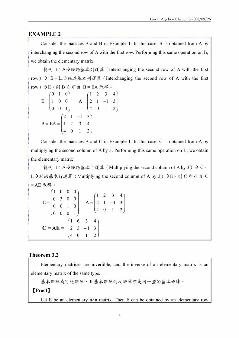
Linear Algebra- Chapter 3 20080926
4
EXAMPLE 2 Consider the matrices A and B in Example 1 In this case B is obtained from A by
interchanging the second row of A with the first row Performing this same operation on I3
we obtain the elementary matrix
範例 1A 經過基本列運算(Interchanging the second row of A with the first
row) BIm 經過基本列運算(Interchanging the second row of A with the first
row) E則 B 亦可由 B = EA 取得
⎟⎟⎟
⎠
⎞
⎜⎜⎜
⎝
⎛=
100001010
E ⎟⎟⎟
⎠
⎞
⎜⎜⎜
⎝
⎛minus=
210431124321
A
⎟⎟⎟
⎠
⎞
⎜⎜⎜
⎝
⎛ minus==
210443213112
EAB
Consider the matrices A and C in Example 1 In this case C is obtained from A by
multiplying the second column of A by 3 Performing this same operation on I4 we obtain
the elementary matrix
範例 1A 經過基本行運算(Multiplying the second column of A by 3) C
In 經過基本行運算(Multiplying the second column of A by 3) E則 C 亦可由 C
= AE 取得
⎟⎟⎟⎟⎟
⎠
⎞
⎜⎜⎜⎜⎜
⎝
⎛
=
1000010000300001
E ⎟⎟⎟
⎠
⎞
⎜⎜⎜
⎝
⎛minus=
210431124321
A
C = AE = ⎟⎟⎟
⎠
⎞
⎜⎜⎜
⎝
⎛minus
210431324361
Theorem 32 Elementary matrices are invertible and the inverse of an elementary matrix is an
elementary matrix of the same type
基本矩陣為可逆矩陣且基本矩陣的反矩陣亦是同一型的基本矩陣
【Proof】
Let E be an elementary ntimesn matrix Then E can be obtained by an elementary row
Linear Algebra- Chapter 3 20080926
5
[column] operation on In By reversing the steps used to transform In into E we can
transform E back into In The result is that In can be obtained from E by an elementary row
[column] operation of the same type By Theorem 31 there is an elementary matrix E
such that nIEE = Therefore E is invertible and 1EE minus=
令 E 是 ntimesn 的基本矩陣E 可由 In 經實施一基本列或行運算取得若把用來實
施 In E 的運算對 E 實施亦可得到 In依據 Theorem 31 可知存在一基本矩陣E
使得 nIEE = 因此 E 為可逆且 1EE minus=
Elementary Matrices Elementary Matrices 1414
An elementary matrix is one that can be obtained from the identity matrix In through a single elementary row operation
⎥⎥⎥
⎦
⎤
⎢⎢⎢
⎣
⎡=
100010001
3I⎥⎥⎥
⎦
⎤
⎢⎢⎢
⎣
⎡=
010100001
1ER2 harr R3
⎥⎥⎥
⎦
⎤
⎢⎢⎢
⎣
⎡=
100050001
2E5R25R2
⎥⎥⎥
⎦
⎤
⎢⎢⎢
⎣
⎡=
100012001
3ER2+ 2R1R2+ 2R1
Operation TOperation T
Elementary Matrices Elementary Matrices 2424
⎥⎥⎥
⎦
⎤
⎢⎢⎢
⎣
⎡=
ihgfedcba
A
AEAfedihgcba
1
010100001
=sdot⎥⎥⎥
⎦
⎤
⎢⎢⎢
⎣
⎡=
⎥⎥⎥
⎦
⎤
⎢⎢⎢
⎣
⎡R2 harr R3
AEAihgfed
cba
2
100050001
555 =sdot⎥⎥⎥
⎦
⎤
⎢⎢⎢
⎣
⎡=
⎥⎥⎥
⎦
⎤
⎢⎢⎢
⎣
⎡5R2
AEAihg
cfbeadcba
3
100012001
222 =sdot⎥⎥⎥
⎦
⎤
⎢⎢⎢
⎣
⎡=
⎥⎥⎥
⎦
⎤
⎢⎢⎢
⎣
⎡+++
R2+ 2R1
Elementary Matrices Elementary Matrices 3434
Each elementary matrix is invertible
1221EI
RR +asymp
⎥⎥⎥
⎦
⎤
⎢⎢⎢
⎣
⎡=
100010021
1E
⎥⎥⎥
⎦
⎤
⎢⎢⎢
⎣
⎡=
100010001
I
IE 2R21R1 minus
asymprArr IEE =12 ie
22R21REI
minusasymp
⎥⎥⎥
⎦
⎤
⎢⎢⎢
⎣
⎡ minus=
100010021
E 1
Elementary Matrices Elementary Matrices 4444
If A and B are row equivalent matrices and A is invertible then B is invertibleSince A and B are row equivalent there exits a sequence of row operations T1hellipTn such that B=TnT1ALet the elementary matrices of these operations be E1hellipEn Thus B=En hellip E2 E1 AThe matrix A En hellipE2 E1 are all invertible
( )( )
1
n
1
3
1
2
1
111
11
1n
1
n
1
3
1
2
1
1
1
n
1
3
1
2
1
11
EEEEABBAEE
EEEAEEEEEA
minusminusminusminusminusminus
minusminus
minusminusminusminusminusminusminusminus
=rArr==
=
3-2 The Rank of a Matrix and Matrix Inverse
In this section we define the rank of a matrix We then use elementary operations to
compute the rank of a matrix and a linear transformation The section concludes with a
procedure for computing the inverse of an invertible matrix
何謂「矩陣的秩(Rank)」利用基本行列運算來計算矩陣與線性轉換的秩本節
還包括介紹如何計算可逆矩陣的反矩陣
Linear Algebra- Chapter 3 20080926
6
DEFINITION 33 Rank of a Matrix
If AisinMmtimesn(F) we define the rank of A denoted rank(A) to be the rank of the linear
transformation LA Fn Fm
若 AisinMmtimesn(F)則矩陣 A 的秩為線性轉換 LA Fn Fm的秩註記為 rank(A)
An ntimesn matrix is invertible if and only if its rank is n
一個 ntimesn 的矩陣為可逆的『若且唯若』條件為該矩陣的 Rank 為 n
Every matrix A is the matrix representation of the linear transformation LA with respect
to the appropriate standard ordered bases Thus the rank of the linear transformation LA is the
same as the rank of one of its matrix representation namely A
每一個矩陣 A 是線性轉換 LA 對於某個標準有序基底的矩陣表示式因此該線性轉
換 LA的 Rank 就等於矩陣表示式 A 的 Rank即 rank(LA) = rank(A)
DEFINITION 29
Let V and W be vector spaces and let T V W be linear If N(T) and R(T) are finite-
dimensional then we define the nullity of T denoted nullity(T) and the rank of T denoted
rank(T) to be the dimensions of N(T) and R(T) respectively
V 與 W 為向量空間且 T V W 為線性轉換
定義 T 的核次數(Nullity)nullity(T) = dimensions of N(T)
定義 T 的秩(Rank)rank(T) = dimension of R(T)
核次數(Nullity)與秩(Rank)分別代表 N(T)與 R(T)的維度
DEFINITION 211
Let β = u1 u2hellip un be an ordered basis for a finite-dimensional vectors space V
For xisinV let a1 a2hellip an be the unique scalars such that
令 β = u1 u2hellip un為有限向量空間 V 的有序基底則存在唯一的一組純量 a1
a2hellip an使得 V 內任意向量均可表達成該組基底的線性組合
sum=
=n
1iiiuax
we define the coordinate vector of x relative to β denoted β[x] by
Linear Algebra- Chapter 3 20080926
7
⎟⎟⎟⎟⎟
⎠
⎞
⎜⎜⎜⎜⎜
⎝
⎛
=β
n
2
1
a
aa
[x] 稱為 x 相對於有序基底 β的座標向量
DEFINITION 212
Suppose that V and W are finite-dimensional vector spaces with ordered bases β = v1
v2hellip vn and γ = w1 w2hellip wn respectively Let T V W be linear Then for each j 1
≦j≦n there exist unique scalars aijisinF 1≦i≦m such that
sum==
m
1iiijj wa)vT( for 1≦j≦n
We call the mtimesn matrix A defined by Aij = aij the matrix representation of T in the ordered bases β and γ and write γ
β= [T]A
If V = W and β = γ then we write β= [T]A
設 V 與 W 分別為有限維度的向量空間β = v1 v2hellip vn與 γ = w1 w2hellip
wn分別為 V 與 W 的有序基底且 T V W 為 V 映至 W 的線性轉換
對每一個 j(1≦ j≦n)而言存在唯一的純量 aij isinF(1≦ i≦m)使得
sum==
m
1iiijj wa)vT(
將 mtimesn 的矩陣 A 定義為 Aij = aij並稱呼 A 為線性轉換 T 的矩陣表達方式在
V 與 W 分別以 β 與 γ作為有序基底下A 可註記為 γβ= [T]A
若 V = W 且 β = γ則 β= [T]A
提示 sum==
m
1iiijj wa)vT( 為「將 vj的像 T(vj)表達成有序基底 γ的線性組合」
DEFINITION 217
Let A be an mtimesn matrix with entries from a field F We denote by LA the mapping LA
Fn Fm defined by LA(x) = Ax (the matrix product A and x) for each column vector xisinFn
We call LA a left-multiplication transformation
令 A 是 mtimesn 的矩陣所有元素均來自 FLA為 Fn映至 Fm的線性轉換並定義為
LA(x) = Ax其中 x 為行向量(Column vector)且 xisinFnLA被稱為左乘法轉換
Linear Algebra- Chapter 3 20080926
8
The next theorem extends this fact to any matrix representation of any linear
transformation defined on finite-dimensional vector spaces
Theorem 33 Let T V W be a linear transformation between finite dimensional vector spaces and
let β and γ be ordered bases for V and W respective Then rank(T) = rank( γβ[T] )
令 T V W且 β 與 γ 分別為有限維度向量空間 V 與 W 的有序基底則
rank(T) = rank( γβ[T] )
改寫 Definition 212
Suppose that Fn and Fm are finite-dimensional vector spaces with ordered bases β =
v1 v2hellip vn and γ = w1 w2hellip wn respectively Let LA Fn Fm be linear and defined
by LA(x) = Ax Then for each j 1≦j≦n there exist unique scalars aijisinF 1≦i≦m such
that sum=
=m
1iiijjA wa)v(L for 1≦j≦n We call the mtimesn matrix A defined by Aij = aij the matrix
representation of LA in the ordered bases β and γ and write γβ= ][LA A
Now that the problem of finding the rank of a linear transformation has been reduced to
the problem of finding the rank of a matrix we need a result that allows us to perform rank-
preserving operations on matrices The next theorem and its corollary tell us how to do this
線性轉換的 Rank 可以被簡化為找矩陣的 Rank如何找矩陣的 Rank
Theorem 34 Let A be an mtimesn matrix If P and Q are invertible mtimesm and ntimesn matrices respectively
then
令 A 為 mtimesn 的矩陣若 P 與 Q 分別為可逆的 mtimesm 與 ntimesn 矩陣則
(a) rank(AQ) = rank(A)
(b) rank(PA) = rank(A)
(c) rank(PAQ) = rank(A)
【Proof】
R(LAQ) = R(LALQ) = LALQ(Fn) = LA(LQ(Fn)) = LA(Fn) = R(LA)
Since LQ is onto rank(AQ) = dim(R(LAQ)) = dim(R(LA)) = rank(A)
Linear Algebra- Chapter 3 20080926
9
rank(PAQ) = rank(PA) = rank(A)
註Theorem 34 是為後續 Reduced Row Echelon Form of Matrix 做準備一個矩陣經過
基本行運算或基本列運算或基本行與列運算後並不會改變 RANK
Corollary
Elementary row and column operations on a matrix are rank-preserving
矩陣的基本列與行運算不會改變矩陣的 Rank
此推論結果是計算反矩陣解線性方程組的重要依據
Theorem 35 The rank of any matrix equals the maximum number of its linearly independent
columns that is the rank of a matrix is the dimension of the subspace generated by its
column
任一矩陣的 Rank 等於其最大線性獨立行向量數目即矩陣的 Rank 是由矩陣的
行向量生成的子空間的維度【LA Fn Fm】
【Proof】
For any AisinMmtimesn(F)
rank(A) = rank(LA) = dim(R(LA))
Let β be the standard basis of Fn Then β spans Fn and hence by Theorem 22
R(LA ) = span(LA (β)) = span(LA(e1) LA(e2)hellip LA(en))
But for any j we have seen in Theorem 213(b) that LA(ej) = Aej = aj where aj is the
jth column of A Hence R(LA ) = span(a1 a2 an)
Thus rank(A) = rank(LA) = dim(span(a1 a2 an))
對任意矩陣 Arank(A) = rank(LA) = dim(R(LA))
令 β為 Fn 的標準基底且生成 Fn
依據 Theorem 22
LA的值域 Range 可由 LA(β)來生成
R(LA) = span(LA (β)) = span(LA(e1) LA(e2)hellip LA(en))
對任意 j 而言由 Theorem 213(b) 可知 LA(ej) = Aej = aj其中aj 為 A 的第 j
個行(aj 相當於 Theorem 213(b)的 vj 或 Theorem 22 的 T(vj))因此 R(LA) =
Linear Algebra- Chapter 3 20080926
10
span(a1 a2 an)
所以 rank(A) = rank(LA) = dimension of R(LA) = dim(span(a1a2an))
Theorem 22 令 V 與 W 為向量空間且 T V W 為線性轉換若 β = v1 v2hellip vn
是定義域(Domain)V 的基底則 T 的值域 Range R(T)可由 T(β)來生成意即 R(T)
= span(T(β)) = span(T(v1) T(v2)hellip T(vn))
Theorem 213 A 為 mtimesn 的矩陣與 B 為 ntimesp 的矩陣uj 與 vj分別為 AB 與 B 的第 j 行
(1 j p≦ ≦ )則
(a) uj = A vj
(b) vj = B ej where ej is the jth standard vector of Fp
EXAMPLE 1
Let ⎟⎟⎟
⎠
⎞
⎜⎜⎜
⎝
⎛=
101110101
A
Observe that the first and second columns of A are linearly independent and that the
third column is a linear combination of the first two Thus
A 的第一行與第二行是線性獨立第三行則是前兩行的線性組合於是
rank(A) = dim⎟⎟⎟⎟
⎠
⎞
⎜⎜⎜⎜
⎝
⎛
⎟⎟⎟
⎠
⎞
⎜⎜⎜
⎝
⎛
⎪⎭
⎪⎬
⎫
⎟⎟⎟
⎠
⎞
⎜⎜⎜
⎝
⎛
⎪⎩
⎪⎨
⎧
⎟⎟⎟
⎠
⎞
⎜⎜⎜
⎝
⎛
⎟⎟⎟
⎠
⎞
⎜⎜⎜
⎝
⎛
111
010
101
span = 2
A 的第 1 行a1=⎟⎟⎟
⎠
⎞
⎜⎜⎜
⎝
⎛
101第 2 行a2=
⎟⎟⎟
⎠
⎞
⎜⎜⎜
⎝
⎛
010第 3 行a3=
⎟⎟⎟
⎠
⎞
⎜⎜⎜
⎝
⎛
111
In order to compute the rank of a matrix A it is frequently useful to postpone the use of
Theorem 35 until A has been suitable modified by means of appropriate elementary row and
column operations so that the number of linearly independent columns is obvious
為了利用 Theorem 35 求矩陣 A 的 Rank(等於最大線性獨立行向量數目)A 可
先經過基本列或行運算使其線性獨立的行數變得比較明顯
EXAMPLE 2 Let
Linear Algebra- Chapter 3 20080926
11
⎟⎟⎟
⎠
⎞
⎜⎜⎜
⎝
⎛=
211301121
A
If we subtract the first row of A from rows 2 and 3 (type 3 elementary row operations)
the result is
⎟⎟⎟
⎠
⎞
⎜⎜⎜
⎝
⎛
minusminus
110220121
If we now substract twice the first column from the second and substract the first
column from the third (type 3 elementary column operations) we obtain
⎟⎟⎟
⎠
⎞
⎜⎜⎜
⎝
⎛
minusminus
110220001
(後二行線性相依最大線性獨立行數為 2)
It is now obvious that the maximum number of linearly independent column of this matrix is 2 Hence the rank of A is 2
Theorem 36 Let A be an mtimesn matrix of rank r Then r m r n and by means of a finite number ≦ ≦
of elementary row and column operations A can be transformed into the matrix
D = ⎟⎟⎠
⎞⎜⎜⎝
⎛
32
1r
OOOI
where O1 O2 and O3 are zero matrices Thus Dii = 1 for i r and ≦
Dij = 0 otherwise
令 A 為 Rank 等於 r 的 mtimesn 矩陣則 r m≦ 且 r n≦ 經過有限次數的基本行與列
運算讓 A 化成 D = ⎟⎟⎠
⎞⎜⎜⎝
⎛
32
1r
OOOI
其中Ir 為對角元素為 1 的對角矩陣即 A 可經
過有限次數的基本行及列運算取得沿對角線前 r 個位置皆為 1其餘各處皆為 0 的
矩陣 D
【Proof】
If A is the zero matrix r = 0 In this case the conclusion follows with D = A
若 A 為零矩陣則 r = 0 且 D = A
Now suppose that AneO and r = rank(A) then r gt 0
The proof is by mathematical induction on m the number of rows of A
若 A 非零矩陣且 r = rank(A)則 r gt 0
Linear Algebra- Chapter 3 20080926
12
採用數學歸納法
Suppose that m = 1
A can be transformed into the matrix (1 0 hellip0)
So rank(D) = rank(A) = 1 by Corollary to Theorem 34 and Theorem 35 Thus the
theorem is established for m = 1
設 m = 1則 A 可以化成(1 0 hellip0)
依據 Corollary to Theorem 34 及 Theorem 35
rank(D) = rank(A) = 1
故本定理對 m = 1 的矩陣是成立的
Next assume that the theorem holds for any matrix with at most m - 1 row (for some m
gt1)
We must prove that the theorem holds for any matrix with m rows
其次假設本定理對至多含 m - 1 列的矩陣皆成立(m gt 1)
至於含 m 列的矩陣是否成立
If n = 1 Theorem 36 can be established in a manner analogous to that for m = 1
若 n = 1則可按 m = 1 的方式證明本定理對於 n = 1 的矩陣成立
We now suppose that n gt 1 Since A ne O Aijne0 for some i j By means of at most one
elementary row and at most one elementary column operation (each of type 1) We can
move the nonzero entry to the 11 position By means of of at most one additional type 2
operation we can assure a 1 in the 11 position By means of at most m ndash 1 type 3 row
operations and at most n ndash 1 type 3 column operations we can eliminate all nonzero entries
in the first row and the first column with the exception of the 1 in the 11 postion
Thus with a finite number of elementary operation A can be transformed into a
matrix
經過有限次數的基本行及列運算可將 A 轉換成
⎪⎪⎭
⎪⎪⎬
⎫
⎪⎪⎩
⎪⎪⎨
⎧
=
0B
0001
B where Brsquo is an (m-1)times(n-1) matrix
Brsquo has rank one less than B
Brsquo的 Rank 比 B 少 1
Since rank(A) = rank(B) = r rank(Brsquo) = r ndash 1 Therefore r ndash1 ≦ m ndash 1 and r ndash1 ≦
Linear Algebra- Chapter 3 20080926
13
n ndash 1 by the induction hypothesis Hence r ≦ m and r ≦ n
由於 rank(A) = rank(B) = r故 rank(Brsquo) = r ndash 1
依數學歸納法 r ndash1 ≦ m ndash 1 且 r ndash1 ≦ n ndash 1
因此 r ≦ m 且 r ≦ n
Also by the induction hypothesis Brsquo can be transformed by a finite number of
elementary row and column operations into the (m-1)times(n-1) matrix Drsquo such that
同樣地依據數學歸納法Brsquo 可經過有限次數的基本行與列運算轉換成 (m-
1)times(n-1) 的矩陣 Drsquo使得
Dlsquo= ⎟⎟⎠
⎞⎜⎜⎝
⎛ minus
65
41r
OOOI
where O4 O5 and O6 are zero matrices
That is Drsquo consists of all zeros except for its first r-1 diagonal entries which are ones
Let
⎪⎪⎭
⎪⎪⎬
⎫
⎪⎪⎩
⎪⎪⎨
⎧
=
0D
0001
D
We see that the theorem now follows once we show that D can be obtained from B by
means of a finite number of elementary row and column operations
D 可由 B 經過有限次基本行及列運算而取得
Thus since A can be transformed into B and B can be transformed into D each by a
finite number of elementary operations A can be transformed into D by a finite number of
elementary operations
經過有限次基本行及列運算A B D
Finally since Drsquo contains ones as its first r ndash 1 diagonal entries D contains ones as its
first r diagonal entries and zeros elsewhere
最後Drsquo沿對角線前 r-1 個位置皆為 1故 D 沿對角線前 r 個位置皆為 1其餘
各處皆為 0
EXAMPLE 3 Consider the maxtrix
⎟⎟⎟⎟⎟
⎠
⎞
⎜⎜⎜⎜⎜
⎝
⎛
=
192362100280844422420
A
Linear Algebra- Chapter 3 20080926
14
By means of a succession of elementary row and column operations we can transform
A into a matrix D as in Theorem 36
透過一系列的基本行與列運算將 A 轉換成 D
D
00000001000001000001
192362100280844422420
A =
⎟⎟⎟⎟⎟
⎠
⎞
⎜⎜⎜⎜⎜
⎝
⎛
==
⎟⎟⎟⎟⎟
⎠
⎞
⎜⎜⎜⎜⎜
⎝
⎛
=
By the corollary to Theorem 34 rank(A) = rank(D) Clearly however rank(D) = 3 so rank(A) = 3
Corollary 1 Let A be an mtimesn matrix of rank r Then there exist invertible matrices B and C of sizes
mtimesm and ntimesn respectively such that D = BAC where D = ⎟⎟⎠
⎞⎜⎜⎝
⎛
32
1r
OOOI
is the mtimesn matrix
in which O1 O2 and O3 are zero matrices
令 A 為 mtimesn 的矩陣Rank 為 r存在可逆的 mtimesm 矩陣 B 與 ntimesn 矩陣 C使得
D = BAC其中D = ⎟⎟⎠
⎞⎜⎜⎝
⎛
32
1r
OOOI
為 mtimesn 的矩陣O1O2 及 O3 為零矩陣
【Proof】
By Theorem 36 A can be transformed by means of a finite number of elementary
row and column operations into the matrix D
We can appeal to Theorem 31 each time we perform an elementary operation Thus
there exist elementary mtimesm matrices E1 E2hellipEp and elementary ntimesn matrices G1
G2hellipGq such that D = EpEp-1hellipE2E1AG1G2hellipGq
By Theorem 32 each Ej and Gj is invertible Let B = EpEp-1hellipE2E1 and C =
G1G2hellipGq Then B and C are invertible and D = BAC
依據 Theorem 36A 可經過有限次的基本列與行運算化成 D
引用 Theorem 31每一次皆實施某一個基本列運算於是存在基本的 mtimesm 矩
陣 E1 E2hellip Ep 與 基 本 的 ntimesn 矩 陣 G1 G2hellip Gq 使 得 D = EpEp-
1hellipE2E1AG1G2hellipGq
依據 Theorem 32 每一個基本矩陣 Ej與 Gj 皆為可逆令 B = EpEp-1hellipE2E1 與 C =
G1G2hellipGq於是 B 與 C 皆為可逆且 D = EpEp-1hellipE2E1AG1G2hellipGq = BAC
Linear Algebra- Chapter 3 20080926
15
Theorem 31 令 AisinMmtimesn(F)並假設 B 是由 A 經實施某一基本列【或行】運算後所得
到的矩陣則存在一個 mtimesm 【或 ntimesn】基本矩陣 E使得 B = EA【或 B = AE】E
矩陣是由 Im 【或 In】 經實施與「由 A 得到 B」相同的基本列【或行】運算後所得
到的矩陣反之若 E 是一個 mtimesm【或 ntimesn】的基本矩陣則 EA【或 AE】是由 A
經過與「由 Im 【或 In】 得到 E」相同的基本列【或行】運算後所得到的矩陣
Theorem 32 基本矩陣為可逆矩陣且基本矩陣的反矩陣亦是同一型的基本矩陣
Theorem 36 令 A 為 Rank 等於 r 的 mtimesn 矩陣則 r m≦ 且 r n≦ 經過有限次數的基
本行與列運算讓 A 化成 D = ⎟⎟⎠
⎞⎜⎜⎝
⎛
32
1r
OOOI
其中Ir為對角元素為 1 的對角矩陣
Corollary 2 Let A be an mtimesn matrix Then
(a) rank(At) = rank(A)
矩陣轉置後的 RANK 不變
(b) The rank of any matrix equals the maximum number of its linearly independent
rows that is the rank of a matrix is the dimension of the subspace generated by
rows
任一矩陣的 Rank 等於最大線性獨立列向量的數目即矩陣的 Rank 等於由該
矩陣列向量所生成的子空間的維度
(c) The rows and columns of any matrix generate subspaces of the same dimension
numerically equal to the rank of the matrix
任一矩陣的列向量與行向量生成的子空間的維度相同維度等於該矩陣的
Rank
【Proof】
By Corollary 1 there exist invertible matrices B and C such that D = BAC where D
satisfies the stated conditions of the corollary Taking transposes we have
Dt = (BAC) t = CtAtBt
Since B and C are invertible so are Bt and Ct
Hence by Theorem 34 rank(At) = rank(CtAtBt) = rank(Dt)
Suppose that r = rank(A)
Then Dt is an ntimesm matrix with the form of the matrix D in Corollary 1 and hence
Linear Algebra- Chapter 3 20080926
16
rank(Dt) = r by Theorem 35
Thus
rank(At) = rank(Dt) = r = rank(A)
依據 Corollary 1存在可逆矩陣 B 與 C使得 D = BAC
取其轉置可得Dt = (BAC) t = CtAtBt
由於 B 與 C 為可逆故 Bt 與 Ct 亦為可逆
依據 Theorem 34得知 rank(At) = rank(CtAtBt) = rank(Dt)
設 r = rank(A)
則 Dt為一 ntimesm 的矩陣型式與 D 相同(參考 Corollary 1)
且依據 Theorem 35 得知 rank(Dt) = r
於是 rank(At) = rank(Dt) = r = rank(A)
Theorem 34 Let A be an mtimesn matrix If P and Q are invertible mtimesm and ntimesn matrices
respectively then 令 A 為 mtimesn 的矩陣若 P 與 Q 分別為可逆的 mtimesm 與 ntimesn 矩陣
則
(a) rank(AQ) = rank(A)
(b) rank(PA) = rank(A)
(c) rank(PAQ) = rank(A)
Theorem 35 The rank of any matrix equals the maximum number of its linearly
independent columns that is the rank of a matrix is the dimension of the subspace
generated by its column 任一矩陣的 Rank 等於其最大線性獨立行向量數目即矩陣
的 Rank 是由矩陣的行向量生成的子空間的維度【LA Fn Fm】
Corollary 3 Every invertible matrix is a product of elementary matrices
每一可逆矩陣均可為基本矩陣的乘積
【Proof】
If A is an invertible ntimesn matrix then rank(A) = n Hence the matrix D in Corollary 1
equals In and there exist invertible matrices B and C such that In = BAC
As in the proof of Corollary 1 note that B = EpEp-1hellipE2E1 and C = G1G2hellipGq where
the Eirsquos and Girsquos are elementary matrices Thus A = B-1InC-1 = B-1C-1 so that
A = E1-1E2
-1hellipEp-1Gq
-1Gq-1-1hellipG1
-1
Linear Algebra- Chapter 3 20080926
17
The inverses of elementary matrices are elementary matrices however and hence A is
the product of elementary matrices
若 A 為可逆的 ntimesn 矩陣則 rank(A) = n
因此 Corollary 1 中的矩陣 D 為 In且存在可逆的 B 與 C 矩陣使得 In = BAC
如同 Corollary 1 的證明一樣B = EpEp-1hellipE2E1 且 C = G1G2hellipGq其中Eirsquos 與
Girsquos 皆為基本矩陣
於是A = B-1InC-1 = B-1C-1即 A = E1-1E2
-1hellipEp-1Gq
-1Gq-1-1hellipG1
-1
基本矩陣的反矩陣亦為基本矩陣A 是基本矩陣的乘積
Theorem 37 Let T V W and U W Z be linear transformations on finite-dimensional vector
spaces V W and Z and let A and B be matrices such that the product AB is defined Then
令 VW 與 Z 為有限維度的向量空間T V W 與 U W Z 為線性轉換且
A 與 B 為滿足乘積 AB 定義的矩陣則
(a) rank(UT) ≦ rank(U)
(b) rank(UT) ≦ rank(T)
(c) rank(AB) ≦ rank(A)
(d) rank(AB) ≦ rank(B)
【Proof】
(a) Clearly R(T)subeW
Hence R(UT) = UT(V) = U(R(T)) sube U(W) = R(U)
Thus rank(UT) = dim(R(UT)) ≦ dim (R(U)) = rank(U)
(c) By (a) rank(AB) = rank(LAB) = rank (LALB) ≦ rank(LA) = rank(A)
(d) By (c) and Corollary 2 to Theorem 36
rank(AB) = rank((AB)t) = rank(B t A t) ≦ rank(B t) = rank (B) (b) Let α β and γ be ordered bases for V W and Z respectively and let Arsquo = γ
β]U[
and Brsquo = βα]T[ Then ArsquoBrsquo = γ
α]UT[ by Theorem 211
Hence by Theorem 33 and (d)
rank(UT) = rank(ArsquoBrsquo) ≦ rank(Brsquo) = rank (T)
Theorem 211 Let V W and Z be finite-dimensional vector space with ordered bases α β
and γ respectively Let T V W and U W Z be linear transformation Then
Linear Algebra- Chapter 3 20080926
18
βα
γβ
γα = [T][U][UT] 令 VW 與 Z 是有限維度的向量空間αβ 與 γ 分別為 VW 與
Z 的有序基底令 T V W (先 α β) 且 U W Z (後 β γ)則 βα
γβ
γα = [T][U][UT]
Theorem 33 Let T V W be a linear transformation between finite dimensional vector
spaces and let β and γ be ordered bases for V and W respective Then rank(T) = rank( γ
β[T] ) 令 T V W且 β 與 γ 分別為有限維度向量空間 V 與 W 的有序基底
則 rank(T) = rank( γβ[T] )
EXAMPLE 4
(a) Let ⎟⎟⎠
⎞⎜⎜⎝
⎛minus
=11111121
A (第一列與第二列是 LI) rank(A) = 2
(b) Let ⎟⎟⎟
⎠
⎞
⎜⎜⎜
⎝
⎛=
003011011131
A (第三列與第一二列是 LD)rank(A) = 2
(c) Let ⎟⎟⎟
⎠
⎞
⎜⎜⎜
⎝
⎛
minus=
011111121321
A (三列為 LI) rank(A) = 3
The inverse of a Matrix
We have remarked that an ntimesn matrix is invertible if and only if its rank is n Since we
know how to compute the rank of any matrix we can always test a matrix to determine
whether it is invertible We now provide a simple technique for computing the inverse of a
matrix that utilizes elementary row operations
已知 ntimesn 矩陣為可逆的『若且唯若』條件為該矩陣的 Rank 等於 n
DEFINITION 34 Augmented Matrix Let A and B be mtimesn and mtimesp matrices respectively By the augmented matrix )BA(
we mean that the mtimes(n+p) matrix )BA( that is the matrix whose first n columns are the
columns of A and whose last p columns are the columns of B 設 A 與 B 分別為 mtimesn 與 mtimesp 的矩陣則增廣矩陣(Augmented matrix) )BA(
Linear Algebra- Chapter 3 20080926
19
為一 mtimes(n+p)的矩陣 )BA( 該矩陣的前 n 行(Column)為 A 的所有的行後 p
行為 B 的所有行
Let A be an invertible ntimesn matrix and consider the ntimes2n augmented matrix C= )IA( n
C= )IA( n )AI()IAAA(CA 1
nn111 minusminusminusminus ==
By Corollary 3 to Theorem 36 A-1 is the product of elementary matrices say
A = EpEp-1hellipE2E1 (A-1 是多個基本矩陣的乘積)
Thus )AI()IAAA(CA 1
nn111 minusminusminusminus == )AI(CA)IA(EEE 1
n1
n11ppminusminus
minus ==
We have the following result If A is an invertible invertible ntimesn matrix then it is
possible to transform the matrix (AIn) into the matrix (InA-1) by means of a finite
number of elementary row operations
若 A 為一可逆的 ntimesn 矩陣則可經過有限次數的基本列運算將矩陣 (AIn) 化成
(InA-1)
Conversely suppose that A is invertible and that for some ntimesn matrix B the matrix
(AIn) can be transformed into the matrix (InB) by a finite number of elementary row
operations Let E1 E2hellip Ep be the elementary matrices associated with these elementary row
operations as in Theorem 31 then
反之假設 A 是可逆且矩陣(AIn)可經有限次數的基本列運算轉換成矩陣(InB)
並令 E1 E2hellip Ep 分別為 Theorem 31 所稱的基本矩陣則
)BI()IA(EEE nn11pp =minus
Let M = EpEp-1hellipE2E1 we have 令 M = EpEp-1hellipE2E1
)BI()IA(EEE nn11pp =minus )BI()IA(M)MMA( nn ==
Linear Algebra- Chapter 3 20080926
20
Hence MA = In and M = B It follows that M = A-1 So B = A-1
可由 MA = In 及 M = B 得知M 就是 A-1故 B 就是 A-1
Thus we have the follow resultsIf A is an invertible ntimesn matrix and the matrix
(AIn) is transformed in a matrix of the form (InB) by means of a finite number of
elementary row operations then B=A-1
若 A 為一可逆的 ntimesn 矩陣且矩陣 (AIn) 可經有限次數的基本列運算化成
(InB)則 B=A-1
If on the other hand A is an ntimesn matrix that is not invertible then rank(A) lt n Hence
any attempt to transform (AIn) into a matrix of the form (InB) by means of elementary row
operations must fail
反之若 A 是一不可逆的 ntimesn 矩陣則 rank(A) lt n因此任何想利用基本列運算
要將矩陣 (AIn) 化成 (InB)的努力必定失敗
Thus we have the follow results If A is an notinvertible ntimesn matrix then any attempt
to transform (AIn) into a matrix of the form (InB) produce a row whose first n entries
are zeros
若 A 是一不可逆的 ntimesn 矩陣任何想將矩陣 (AIn) 化成 (InB)的努力最後會
產生一前 n 個元素均為 0 的列
EXAMPLE 5
We determine whether the matrix ⎟⎟⎟
⎠
⎞
⎜⎜⎜
⎝
⎛=
133242420
A is invertible and if it is we
compute its inverse
A 是否為可逆矩陣
We attempt to use elementary row operations to transfer
Linear Algebra- Chapter 3 20080926
21
⎟⎟⎟
⎠
⎞
⎜⎜⎜
⎝
⎛=
100010001
133242420
)IA( into a matrix of the form (InB)
看看能否利用基本行與列運算將矩陣 (AIn) 化成 (InB)
Interchanging rows 1 and 2
⎟⎟⎟
⎠
⎞
⎜⎜⎜
⎝
⎛
100001010
133420242
Multiplying the first row by 12
⎟⎟⎟
⎠
⎞
⎜⎜⎜
⎝
⎛
10000100
133420121 2
1
Adding -3 times row 1 to row 3
⎟⎟⎟
⎠
⎞
⎜⎜⎜
⎝
⎛
minusminusminus 1000100
230420121
23
21
Multiplying row 2 by 12 to obtain 1 in the 22 position
⎟⎟⎟
⎠
⎞
⎜⎜⎜
⎝
⎛
minus
minus
minusminus 100000
230210121
23
21
21
Adding -2 times row 2 to row 1 and 3 times row 2 to row 3
⎟⎟⎟
⎠
⎞
⎜⎜⎜
⎝
⎛
minus
minusminus
10001
400210301
23
2321
21
Multiplying row 3 by 14
⎟⎟⎟
⎠
⎞
⎜⎜⎜
⎝
⎛
minus
minusminus
41
83
8321
21
0001
100210301
Adding appropriate multiply of row 3 to row 1 and 2 completes the process
⎟⎟⎟
⎠
⎞
⎜⎜⎜
⎝
⎛
minusminus
minus
41
83
83
21
43
41
43
85
81
100010001
目標達成
Thus A is invertible and ⎟⎟⎟
⎠
⎞
⎜⎜⎜
⎝
⎛
+minus+minus+minus+minus+
=minus
41
83
83
21
43
41
43
85
81
1A
Linear Algebra- Chapter 3 20080926
22
EXAMPLE 6
We determine whether the matrix ⎟⎟⎟
⎠
⎞
⎜⎜⎜
⎝
⎛minus=451112
121A is invertible and if it is we
compute its inverse
A 是否為可逆矩陣
We attempt to use elementary row operations to transfer
⎟⎟⎟
⎠
⎞
⎜⎜⎜
⎝
⎛minus=
100010001
451112
121)IA( into a matrix of the form (InB)
看看能否利用基本行與列運算將矩陣 (AIn) 化成 (InB)
Adding -2 times row 1 to row 2 and -1 times row 1 to row 3 then addig row 2 to row
3
⎟⎟⎟
⎠
⎞
⎜⎜⎜
⎝
⎛minus
100010001
451112
121
⎟⎟⎟
⎠
⎞
⎜⎜⎜
⎝
⎛
minusminusminusminus
101012001
330330
121
⎟⎟⎟
⎠
⎞
⎜⎜⎜
⎝
⎛
minusminusminusminus
113012001
000330
121
is a matrix with row whose first 3 entries are zeros Therefore A is not invertible
最後一列前 3 個元素均為 0
EXAMPLE 7 Let T P2(R) P2(R) be defined by T(f(x)) = f(x)+frsquo(x)+frdquo(x) where frsquo(x) and frdquo(x)
denote the first and second derivatives of f(x) We use Corollary 1 to Theorem 218 to test
T for invertibility and compute the inverse if T is invertible Taking β=1 x x2 to be the
standard ordered basis of P2(R) we have
令 T P2(R) P2(R) 為線性轉換且定義為 T(f(x)) = f(x)+frsquo(x)+frdquo(x)利用
Corollary 1 to Theorem 218 來測試 T 是否可逆並計算其逆轉換取 β=1 x x2為
P2(R)的標準有序基底
T(1) = 1 = 1bull1+0bullx+0bullx2
T(x) = 1+x = 1bull1+1bullx+0bullx2
Linear Algebra- Chapter 3 20080926
23
T(x2) = 2+2x+x2 = 2bull1+2bullx+1bullx2
⎟⎟⎟
⎠
⎞
⎜⎜⎜
⎝
⎛=β
100210211
[T] 稱為 T 相對有序基底 β的座標向量
依據 Corollary 1 to Theorem 218 T 可逆『若且唯若』 β[T] 可逆且
1-1 )[T](][T minusββ =
Using the method of Examples 5 and 6 we can show that β[T] is invertible with
inverse
⎟⎟⎟
⎠
⎞
⎜⎜⎜
⎝
⎛minus
minus=minus
β
100210
011)([T] 1
Thus T is is invertible and βminusminus
β = ][T)([T] 11 Hence by Theorem 214 we have
⎟⎟⎟
⎠
⎞
⎜⎜⎜
⎝
⎛minusminus
=⎟⎟⎟
⎠
⎞
⎜⎜⎜
⎝
⎛
⎟⎟⎟
⎠
⎞
⎜⎜⎜
⎝
⎛minus
minus=++ β
minus
2
21
10
2
1
02
2101
aa2aaa
aaa
100210
011)]xaxa(a[T
Therefore T-1(a0+a1x+a2x2) = (a0-a1)+(a1-2a2)x+a2x2 Corollary 1 to Theorem 218 Let V be finite-dimensional vector space with an ordered basis β and let T V V be linear Then T is invertible if and only if β[T] is invertible
Furthermore 1-1 )[T](][T minusββ = V 為有限維度的向量空間β 是 V 的有序基底令 T
V V 為線性轉換 T 為可逆的『若且唯若』條件為 β[T] 可逆再者
1-1 )[T](][T minusββ =
Theorem 214 Let V and W be finite-dimensional vector spaces having ordered bases β and γ respectively and let T V W be linear Then for each uisinV we have β
γβγ = [u][T][T(u)]
V 與 W 為有限維度的向量空間β 與 γ分別 V 與 W 的有序基底令 T V W 為線
性轉換則 V 中的 u 映至 W 的結果 T(u) 相對於有序基底 γ 的座標向量為
βγβγ = [u][T][T(u)]
Invertible and Inverse of MATRIX Let A be an n times n matrix If a matrix B can be found such that AB = BA = In then A is
Linear Algebra- Chapter 3 20080926
24
said to be invertible and B is called the inverse of A (denote B = A-1 and A-k=(A-1)k )
If such a matrix B does not exist then A has no inverse
EXAMPLE
⎥⎦
⎤⎢⎣
⎡=
4321
A and ⎥⎦
⎤⎢⎣
⎡minus
minus=
21
23
12B
221
23
221
23
I1001
432112
BA
I100112
4321
AB
=⎥⎦
⎤⎢⎣
⎡=⎥
⎦
⎤⎢⎣
⎡⎥⎦
⎤⎢⎣
⎡minus
minus=
=⎥⎦
⎤⎢⎣
⎡=⎥
⎦
⎤⎢⎣
⎡minus
minus⎥⎦
⎤⎢⎣
⎡=
Thus AB = BA = I2 proving that the matrix A has inverse B
Theorem The inverse of an invertible matrix is unique
Let B and C be inverse of A
Thus AB = BA = In and AC = CA = In
Multiply both sides of the equation AB = In by C
C(AB) = CIn (CA)B = C
InB = C B = C
Thus an invertible matrix has only one inverse
How to find AHow to find A--11
Based on the GaussBased on the Gauss--Jordan algorithmJordan algorithmLet A be an invertible matrix Then AALet A be an invertible matrix Then AA--11=I=Inn
Let the columns of Let the columns of AA--11 be be XX11 XX22 helliphellip XXnn and the columns of I and the columns of Inn be be CC11CC22helliphellipCCnn
Find AFind A--11 by finding by finding XX11 XX22 helliphellip XXnn Write the equation AAWrite the equation AA--11=I=Inn in the formin the form
[ ] [ ]n21nn211 CCCI XXXALet LL ==minus
[ ] [ ][ ] [ ]n21n21
n21n21
CCCAXAXXACCCXXXALL
LL
=rArr=
nn2211 CAXCAX CAX === LThus
How to find AHow to find A--11
Solving these systems by using Gauss-Jordan elimination on the large augmented matrix [AC1 C2hellipCn]
Thus when A-1 exits
[ ] [ ] [ ] 1n
1nn ABwhereBIAIIA minusminus ==asympasympL
If the reduced echelon form of [If the reduced echelon form of [AIAInn] is computed and ] is computed and the first part is not of the form Ithe first part is not of the form Inn then A has no inversethen A has no inverse
[ ][ ]n21n
n21
XXXI CCCAmatrix augmented
LL
L
asympasymp
Linear Algebra- Chapter 3 20080926
25
Example Example 1212
⎥⎥⎥
⎦
⎤
⎢⎢⎢
⎣
⎡
minusminusminusminusminus
=100531010532001211
]IA[ 3
⎥⎥⎦
⎤
⎢⎢⎣
⎡minusminusminus
minusminus
+minus+
asymp
101320012110001211
1RR1R3
2)(R2
⎥⎥⎦
⎤
⎢⎢⎣
⎡minus
minusminusminusasymp
101320012110001211
R2)1(
⎥⎥⎥
⎦
⎤
⎢⎢⎢
⎣
⎡
minusminusminusminusminus
=531532211
ADetermine the inverse of
Example Example 2222
⎥⎥⎦
⎤
⎢⎢⎣
⎡
minusminusminusminus
minus++asymp
123100012110013101
R2)2(R3R2R1
⎥⎥⎦
⎤
⎢⎢⎣
⎡
minusminusminus
minus++asymp
123100135010010001
R3)1(R2R3R1
123135110
A 1
⎥⎥⎥
⎦
⎤
⎢⎢⎢
⎣
⎡
minusminusminus=minus
⎥⎥⎦
⎤
⎢⎢⎣
⎡
minusminus
minus
+minus+asymp
135000011210012301
3R2R3R2)1(R1
ExampleExampleDetermine the inverse of
⎥⎥⎦
⎤
⎢⎢⎣
⎡
minus=
412721511
A
⎥⎥⎦
⎤
⎢⎢⎣
⎡
minus=
100412010721001511
][ 3IA
⎥⎥⎦
⎤
⎢⎢⎣
⎡
minusminusminusminus
minus+minus+asymp
102630011210001511
R1)2(R31)R1(R2
There is no need to proceed further There is no need to proceed further The reduced echelon form cannot have a one in the (3 3) locatioThe reduced echelon form cannot have a one in the (3 3) location n
The reduced echelon form cannot be of the form [IThe reduced echelon form cannot be of the form [Inn B] B] Thus Thus AAndashndash11 does not existdoes not exist
Properties of Matrix InverseProperties of Matrix Inverse
Let Let AA and and BB be invertible matrices andbe invertible matrices and cc a nonzero scalar a nonzero scalar ThenThen
AA =minusminus 11)( 111 1)( 2 minusminus = A
ccA
111)( 3 minusminusminus = ABAB
nn AA )()( 4 11 minusminus =tt AA )()( 5 11 minusminus =
Color Models Color Models 1212
A color model in the context of graphics is a method of A color model in the context of graphics is a method of implementing colorsimplementing colorsThe common used models include RGB model and YIQ modelThe common used models include RGB model and YIQ modelThe RGB model is used in computer monitors and the YIQ model The RGB model is used in computer monitors and the YIQ model is used in television screensis used in television screensAn RGB computer signal can be converted to a YIQ television An RGB computer signal can be converted to a YIQ television signal using the matrix transformationsignal using the matrix transformation
⎥⎥⎥
⎦
⎤
⎢⎢⎢
⎣
⎡
⎥⎥⎥
⎦
⎤
⎢⎢⎢
⎣
⎡
minusminusminus=
⎥⎥⎥
⎦
⎤
⎢⎢⎢
⎣
⎡
BGR
311523212321275596
114587299
QIY
YIQgtRGBYIQgtRGB
Color Models Color Models 2222
A signal is converted from a television screen to a computer monA signal is converted from a television screen to a computer monitor itor using inverse of the above matrixusing inverse of the above matrix
⎥⎥⎥
⎦
⎤
⎢⎢⎢
⎣
⎡
⎥⎥⎥
⎦
⎤
⎢⎢⎢
⎣
⎡
minusminusminus=
⎥⎥⎥
⎦
⎤
⎢⎢⎢
⎣
⎡rArr
⎥⎥⎥
⎦
⎤
⎢⎢⎢
⎣
⎡
⎥⎥⎥
⎦
⎤
⎢⎢⎢
⎣
⎡
minusminusminus=
⎥⎥⎥
⎦
⎤
⎢⎢⎢
⎣
⎡minus
QIY
0751108116472721
6209561
BGR
QIY
311523212321275596
114587299
BGR 1
CryptographyCryptography 密碼學密碼學 1212
Cryptography is the process of coding and decoding messagesCryptography is the process of coding and decoding messagesThe technique can be traced back to the ancient Greeks Today The technique can be traced back to the ancient Greeks Today governments use sophisticated methods of coding and decoding governments use sophisticated methods of coding and decoding messagesmessagesOne type of code that is extremely difficult to break makes use One type of code that is extremely difficult to break makes use of a of a large matrix to encode a message large matrix to encode a message The receiver of the message decodes it using the inverse of the The receiver of the message decodes it using the inverse of the matrixmatrixThe first matrix is called the encoding matrix and its inverse The first matrix is called the encoding matrix and its inverse is is called the decoding matrixcalled the decoding matrix
Cryptography Cryptography 密碼學密碼學 2222
A A-1Message
Encoding MatrixEncoding Matrix
Decoded MessageTransmission
Decoding MatrixDecoding Matrix
Linear Algebra- Chapter 3 20080926
26
Example Example 1212
Let the message be Let the message be BUY IBM STOCKBUY IBM STOCKAnd the encoding matrix beAnd the encoding matrix be
⎥⎥⎥
⎦
⎤
⎢⎢⎢
⎣
⎡ minusminusminus
434110433
B U Y B U Y -- I B M I B M -- S T O C KS T O C K2 21 25 27 9 2 13 27 19 20 15 3 112 21 25 27 9 2 13 27 19 20 15 3 11
⎥⎥⎥
⎦
⎤
⎢⎢⎢
⎣
⎡ minusminusminusminusminus=
⎥⎥⎥
⎦
⎤
⎢⎢⎢
⎣
⎡
⎥⎥⎥
⎦
⎤
⎢⎢⎢
⎣
⎡ minusminusminus
2331372091431715418461146
222117196116169
27319225271527921112013272
434110433
EncodingEncoding
Example Example 2222
Let the message be Let the message be BUY IBM STOCKBUY IBM STOCKAnd the decoding matrix beAnd the decoding matrix be
⎥⎥⎥
⎦
⎤
⎢⎢⎢
⎣
⎡
minusminus 334344101
B U Y B U Y -- I B M I B M -- S T O C KS T O C K2 21 25 27 9 2 13 27 19 20 15 3 112 21 25 27 9 2 13 27 19 20 15 3 11
⎥⎥⎥
⎦
⎤
⎢⎢⎢
⎣
⎡=
⎥⎥⎥
⎦
⎤
⎢⎢⎢
⎣
⎡ minusminusminusminusminus
⎥⎥⎥
⎦
⎤
⎢⎢⎢
⎣
⎡
minusminus 27319225271527921112013272
2331372091431715418461146
222117196116169
334344101
DecodingDecoding
3-3 Systems of Linear Equations ndash Theoretical Aspects
The system of equations
mnmn22m11m
2nn2222121
1nn1212111
bxaxaxa
bxaxaxabxaxaxa
=+++
=+++=+++
(S)
were aij and bi (1≦i≦m and 1≦j≦n) are scalars in a field F and x1 x2hellipxn are n
variables taking values in F is called a system of m linear equations in n unknows over the
field F
上式稱為佈於 Field F 含有 n 個未知數m 個線性方程式的系統或方程組(system
of m linear equations in n unknows)
The mtimesn matrix
⎟⎟⎟⎟⎟
⎠
⎞
⎜⎜⎜⎜⎜
⎝
⎛
=
mn2m1m
n22221
n11211
aaa
aaaaaa
A is called the coefficient matrix of the
system (S)(係數矩陣) If we let
⎟⎟⎟⎟⎟
⎠
⎞
⎜⎜⎜⎜⎜
⎝
⎛
=
n
2
1
x
xx
x and
⎟⎟⎟⎟⎟
⎠
⎞
⎜⎜⎜⎜⎜
⎝
⎛
=
m
2
1
b
bb
b Then the system (S) may
be rewritten as a single matrix equation Ax = b(單一矩陣方程式)
To exploit the results that we have developed we often consider a system of linear
equations as a single matrix equation
Linear Algebra- Chapter 3 20080926
27
A solution to the system (S) is an n-tuple n
n
2
1
F
s
ss
s isin
⎟⎟⎟⎟⎟
⎠
⎞
⎜⎜⎜⎜⎜
⎝
⎛
= such that As = b The set of
all solutions to the system (S) is called the solution set of the system(解集合) System (S)
is called consistent(相容) if its solution set is nonempty otherwise it is called
inconsistent(不相容)
方程組(S)的解為一 n 序組該序組可以使 As = b方程組的所有解所成的集合
稱為該方程組的解集合(Solution set)方程組的解集合非空集合者稱為「相容」解
集合空集合者稱為「不相容」
EXAMPLE 1
Consider 6x2xx1xx3x2
321
321
=+minus=++
that is ⎟⎟⎠
⎞⎜⎜⎝
⎛=
⎟⎟⎟
⎠
⎞
⎜⎜⎜
⎝
⎛
⎟⎟⎠
⎞⎜⎜⎝
⎛minus 6
1
xxx
211132
3
2
1
(以矩陣表示)
This system has many solutions such as ⎟⎟⎟
⎠
⎞
⎜⎜⎜
⎝
⎛minus=
726
s and ⎟⎟⎟
⎠
⎞
⎜⎜⎜
⎝
⎛
minusminus=
34
8s
Consider 1xx0xx
21
21
=+=+
that is ⎟⎟⎠
⎞⎜⎜⎝
⎛=⎟⎟
⎠
⎞⎜⎜⎝
⎛⎥⎦
⎤⎢⎣
⎡10
xx
1111
2
1
顯然地方程組無解
We begin our study of system of linear equations by examining the class of
homogeneous system of linear equations 先討論齊次方程組
DEFINITION 35 Homogeneous amp Nonhomogeneous
A system Ax=b of m linear equations in n unknowns is said to be homogeneous if b=0
Otherwise the system is said to be nonhomogeneous
方程組 Ax = bb = 0 稱為齊次方程組否則稱為非齊次方程組
Any homogeneous system has at least one solution namely the zero vector The next
result gives further information about the set of solutions to a homogeneous system
Linear Algebra- Chapter 3 20080926
28
齊次方程組至少有一個解那就是『零向量』
Theorem 38 Let Ax = 0 be a homogeneous system of m linear equations in n unknowns over a field
F Let K denote the set of all solutions to Ax = 0 Then K = N(LA) hence K is a subspace
of Fn of dimension n - rank(LA) = n- rank(A)
令 Ax = 0 代表一佈於 Field 含有 n 個未知數m 個線性方程式的方程組若令
K 代表該方程組的解集合(Solution set)則 K = N(LA)K 為 Fn 內的子空間且其維
度為 n ndash rank (LA) = n - rank(A)
【Proof】
Clearly K = sisinFn As = 0 = N(LA) The second part now follows from the
dimension theorem
Nullity(T)+rank(T) = dim(V)
Nullity (LA) = dim (Fn) ndashrank (LA ) = n ndash rank (A)
DEFINTION 27 Let V and W be vector space and let T V W be linear We define
the null space (or kernel) N(T) of T to be the set of all vectors x in V such that T(x) = 0
that is N(T) = xisinV T(x) = 0 V 與 W 為向量空間且 T V W 為線性轉換定義
線性轉換 T 的 Null space 為 V 內所有滿足 T(x) = 0 的向量 x 所形成的集合註記為
N(T)Null space 的元素 x 經線性轉換 T 轉換後所對應的「像」為 0意即 T(x) = 0
Null space 內的元素的「像」皆為 0
DEFINITION 217 Let A be an mtimesn matrix with entries from a field F We denote by LA
the mapping LA Fn Fm defined by LA(x) = Ax (the matrix product A and x) for each
column vector xisinFn We call LA a left-multiplication transformation 令 A 是 mtimesn
的矩陣所有元素均來自 FLA 為 Fn 映至 Fm的線性轉換並定義為 LA(x) = Ax其中
x 為行向量(Column vector)且 xisinFnLA被稱為左乘法轉換
Theorem 23 (Dimension Theorem) Let V and W be vector spaces and let T V W be
linear If V is finite-dimensional then Nullity(T) + rank(T) = dim(V) T 的核次數
(Nullity)與秩(Rank)的和等於定義域的維度 dim(V)
Corollary Let Ax = 0 be a homogeneous system of m linear equations in n unknowns over a field
Linear Algebra- Chapter 3 20080926
29
F If m lt n the system Ax = 0 has a nonzero solution
令 Ax = 0 代表一佈於 Field 含有 n 個未知數m 個線性方程式的方程組若 m
lt n則該方程組具有一非零解
【Proof】
Suppose that m lt n Then rank(A) = rank (LA)≦m Hence dim(K) = n - rank(LA) ≧
n ndash m gt 0 where K = N(LA) Since dim(K) gt 0 Kne 0 Thus there exists a nonzero
vector sisinK so s is a nonzero solution to Ax = 0
設 m lt n則 rank(A) = rank (LA) ≦ m依據 Theorem 38K = sisinFn As = 0
= N(LA) = dim(K) = n - rank(LA) ≧ n ndash m gt 0表示 dim(K) gt 0Kne 0故存在非
零向量 s使得 Ax = 0
EXAMPLE 2
Consider 0xxx
0xx2x
321
321
=minusminus=++
Let ⎟⎟⎠
⎞⎜⎜⎝
⎛minusminus
=111
121A be the coefficient matrix of this system It is clear that rank(A)
= 2 If K is the solution set of this system then dim(K) = 3-2 = 1 Thus any nonzero
solution constitutes a basis for K
若 K 是方程組的解所組成的集合(簡稱為解集合)依 Theorem 38 得知 dim(K)
= 3 - 2 = 1因此任一非零解將形成 K 的基底
For example since ⎟⎟⎟
⎠
⎞
⎜⎜⎜
⎝
⎛minus32
1 is a solution to the given system
⎪⎭
⎪⎬
⎫
⎪⎩
⎪⎨
⎧
⎟⎟⎟
⎠
⎞
⎜⎜⎜
⎝
⎛minus32
1 is a basis for
K Thus any vector in K is of the form ⎟⎟⎟
⎠
⎞
⎜⎜⎜
⎝
⎛minus=
⎟⎟⎟
⎠
⎞
⎜⎜⎜
⎝
⎛minus
t3t2
t
32
1t where tisinR
例如因⎟⎟⎟
⎠
⎞
⎜⎜⎜
⎝
⎛minus32
1是方程組的一個解故
⎪⎭
⎪⎬
⎫
⎪⎩
⎪⎨
⎧
⎟⎟⎟
⎠
⎞
⎜⎜⎜
⎝
⎛minus32
1 為 K 的基底K 內的任一向量均
具有如下形式
⎟⎟⎟
⎠
⎞
⎜⎜⎜
⎝
⎛minus=
⎟⎟⎟
⎠
⎞
⎜⎜⎜
⎝
⎛minus
t3t2
t
32
1t
Linear Algebra- Chapter 3 20080926
30
We now turn to the study of nonhomogeneous systems Our next result shows that the
solution set of a nonhomogeneous system Ax = b can be described in terms of the solution of
the homogeneous system Ax = 0 We refer to the equation Ax = 0 as the homogeneous system
corresponding to Ax = b
以下將進一步探討「非齊次方程組」非齊次方程組 Ax = b 的解集合可利用齊次方
程組 Ax = 0 的解來加以說明因此我們可將 Ax = 0 視為 Ax = b 的齊次方程組
Theorem 39 Let K be the solution set of a system of linear equations Ax = b and let KH be the
solution set of the corresponding homogeneous system Ax = 0 Then for any solution s to
Ax = b K =s + KH = s+k kisinKH
設 K 為線性方程組 Ax = b 的解集合且 KH為對應的齊次方程組的解集合則
對 Ax = b 的任一個解 s 而言K =s + KH = s+k kisinKH
【Proof】
Let s be any solution to Ax = b
We must show that K =s + KH
If wisinK then Aw = b Hence
A(w - s) = Aw ndash As = b ndash b = 0
So w - sisinKH
Thus there exists kisinKH such that w - s = k
It follows that w = s + k isin s +KH and therefore Ksube s +KH
Conversely suppose that wisins +KH then w = s + k for some kisinKH
But then Aw = A(s + k) = As + Ak = b + 0 = b so wisinK
Therefore s +KHsubeK and thus K=s +KH
令 s 為 Ax = b 的任一個解我們必須證明「K =s + KH」
若 wisinK則 Aw = b(即 w 為 Ax = b 的解)
於是 A(w - s) = Aw ndash As = b ndash b = 0
所以 w - sisinKH(即 w-s 為 Ax = 0 的解)
w - s 既然是 KH的元素表示有一元素 kisinKH使得 w - s = kw = s + k
w = s + kisins +KH
Linear Algebra- Chapter 3 20080926
31
因此 Ksube s +KH
反之假設 wisins +KH則 KH中存在一元素 k(kisinKH)使得 w = s + k
因 Aw = A(s + k) = As + Ak = b + 0 = b
故 wisinK 是 Ax = b 的解
因此s +KHsubeK
總結K=s +KH
EXAMPLE 3
Consider 4xxx7xx2x
321
321
minus=minusminus=++
The corresponding homogeneous system is the system in Example 2 It is easily
verified that ⎟⎟⎟
⎠
⎞
⎜⎜⎜
⎝
⎛=
411
s is a solution to the preceeding nonhomogeneous system So the
solution set of the system is ⎪⎭
⎪⎬
⎫
⎪⎩
⎪⎨
⎧isin
⎟⎟⎟
⎠
⎞
⎜⎜⎜
⎝
⎛minus+
⎟⎟⎟
⎠
⎞
⎜⎜⎜
⎝
⎛= Rt
32
1t
411
K by Theorem 39
⎟⎟⎟
⎠
⎞
⎜⎜⎜
⎝
⎛=
411
s 是非齊次方程組 Ax = b 的解
⎟⎟⎟
⎠
⎞
⎜⎜⎜
⎝
⎛minus32
1是齊次方程組的解
依據 Theorem 39 得知線性方程組 Ax = b 的解集合⎪⎭
⎪⎬
⎫
⎪⎩
⎪⎨
⎧isin
⎟⎟⎟
⎠
⎞
⎜⎜⎜
⎝
⎛minus+
⎟⎟⎟
⎠
⎞
⎜⎜⎜
⎝
⎛= Rt
32
1t
411
K
The following theorem will provide us with a means of computing solutions to certain
system of linear equations
Theorem 310~311 提供計算線性方程組的解的方法
Theorem 310 Let Ax = b be a system of n linear equations in n unknowns If A is invertible then the
Linear Algebra- Chapter 3 20080926
32
system has exactly one solution namely A-1b Conversely if the system has exactly one
solution then A is invertible
令 Ax = b 為含 n 個未知數n 個線性方程式的方程組若 A 為可逆則方程組
恰有一個解解為 A-1b反之若該方程組恰有一個解則 A 為可逆
【Proof】
Suppose that A is invertible
Substituting A-1b into system we have A(A-1b)=( AA-1)b = b
Thus A-1b is a solution
If s is an arbitrary solution then As = b
Multiplying both sides by A-1 gives s= A-1b
Thus the system has one and only one solution namely A-1b
假設 A 為可逆將 A-1b 代入方程組可得 A(A-1b)=( AA-1)b = b
故 A-1b 確為方程組的解
若 s 為方程組的任意解則 As = b
兩邊乘上 A-1可得 s= A-1b
因此方程組僅有唯一的解 A-1b
Conversely suppose that the system has exactly one solution s
Let KH denot the solution set for the corresponding homogeneous system Ax = 0
By Theorem 39 s = s + KH But it is so only if KH = 0 Thus N(LA) = 0 and
hence A is invertible
反之假設方程組恰有一個解 s
令 KH為相對應齊次方程組 Ax = 0 的解集合
依據 Theorem 39要能s = s + KH唯有 KH = 0
KH = 0即表示 N(LA) = 0故 A 為可逆
EXAMPLE 4 Consider the following system of three linear equations in three unknowns
1xx3x33x2x4x2
2x4x2
321
321
32
=++=++
=+
In Example 5 of Section 32 we compute the inverse of the coefficient matrix A of
this system Thus the system has exactly one solution namely
Linear Algebra- Chapter 3 20080926
33
⎟⎟⎟
⎠
⎞
⎜⎜⎜
⎝
⎛=
133242420
A⎟⎟⎟
⎠
⎞
⎜⎜⎜
⎝
⎛
+minus+minus+minus+minus+
=minus
41
83
83
21
43
41
43
85
81
1A
⎟⎟⎟
⎠
⎞
⎜⎜⎜
⎝
⎛
minus+minus
=⎟⎟⎟
⎠
⎞
⎜⎜⎜
⎝
⎛
⎟⎟⎟
⎠
⎞
⎜⎜⎜
⎝
⎛
+minus+minus+minus+minus+
==⎟⎟⎟
⎠
⎞
⎜⎜⎜
⎝
⎛minus
814587
41
83
83
21
43
41
43
85
81
1
3
2
1
132
bAxxx
Theorem 311 Let Ax = b be a system of linear equations Then the system is consistent (相容)if
and only if rank(A) = rank (A∣b) Matrix (A b) is called the augmented matrix o∣ f the
system Ax = b
令 Ax = b 為線性方程式方程組則此方程組至少有一個解的『若且唯若』條件
為 rank(A) = rank (A∣b) 矩陣(A∣b)稱為方程組 Ax = b 的增廣矩陣
【Proof】
To say that Ax = b has a solution is equivalent to saying that bisinR(LA)
In the proof of Theorem 35 we saw that R(LA ) = span(a1 a2 an) the span of the
column of A
Thus Ax = b has a solution if and only if bisinspan(a1 a2 an)
But bisinspan(a1 a2 an) if and only if span(a1 a2 an) = span(a1 a2 an b)
This last statement is equivalent to
dim (span(a1a2an)) = dim (span(a1a2an b))
So by Theorem 35 the preceeding equation reduces to rank(A) = rank (A∣b)
Ax = b 有一解相當於 bisinR(LA)即 b 屬於線性轉換 LA的 Range
在 Theorem 35 的證明中提到 R(LA ) = span(a1a2an)aj 為 A 的第 j 個行
(Column)即線性轉換 LA 的 Range 係由矩陣 A 的行(Column)所生成
因此 Ax = b 要有一個解的『若且唯若』條件為 bisinspan(a1 a2 an)
至於 bisinspan(a1 a2 an)之條件
bisinspan(a1a2an) 的『若且唯若』條件為 span(a1a2an) = span(a1a2an
b)
其條件相當於
Linear Algebra- Chapter 3 20080926
34
dim (span(a1a2an)) = dim (span(a1a2an b))
依據 Theorem 35該條件可簡化為 rank(A) = rank (A∣b)
Theorem 35 The rank of any matrix equals the maximum number of its linearly
independent columns that is the rank of a matrix is the dimension of the subspace
generated by its column任一矩陣的 Rank 等於其最大線性獨立行向量數目即矩陣的
Rank 是由矩陣的行向量生成的子空間的維度【LA Fn Fm】
EXAMPLE 5 Recall the system of equations
1xx0xx
21
21
=+=+
Since ⎟⎟⎠
⎞⎜⎜⎝
⎛=
1111
A and ⎟⎟⎠
⎞⎜⎜⎝
⎛=
111011
)bA(
rank(A) = 1 and rank (A b) = 2∣
Because the two ranks are unequal the system has no solutions
矩陣 A 與增廣矩陣(A∣b) 的 Rank 不同故方程組沒有解
EXAMPLE 6 We can use Theorem 311 to determine whether (3 3 2) is in the range of the linear
transformation T R3 R3 defined by T(a1 a2 a3) = (a1+a2+a3 a1-a2+a3 a1+a3)
利用 Theorem 311 來判斷 (3 3 2)是否在線性轉換 T 的 Range 中其中T R3
R3 定義為 T(a1 a2 a3) = (a1+a2+a3 a1-a2+a3 a1+a3)
Now (3 3 2)isinR(T) if and only if there exists a vector s = x1 x2 x3 in R3 such that
T(s)=(3 3 2) Such a vector s must be a solution to the system
2xx3xxx3xxx
31
321
321
=+=+minus=++
Since the ranks of the coefficient matrix and the augmented matrix of this system
are 2 and 3 respectively it follows that this system has no solutions Hence (3 3 2) notin
R(T)
(3 3 2)isinR(T) 的『若且唯若』的條件為存在一向量 s = x1 x2 x3isinR3 使得
T(s)=(3 3 2)
Linear Algebra- Chapter 3 20080926
35
向量 s 必須是 2xx3xxx3xxx
31
321
321
=+=+minus=++
的解
因係數矩陣⎟⎟⎟
⎠
⎞
⎜⎜⎜
⎝
⎛minus
101111111
的 Rank 為 2增廣矩陣⎟⎟⎟
⎠
⎞
⎜⎜⎜
⎝
⎛minus
233
101111111
的 Rank 為 3兩
者不相等故方程組無解(3 3 2) notin R(T)
Theorem 311 Let Ax = b be a system of linear equations Then the system is consistent
(相容)if and only if rank(A) = rank (A∣b) Matrix (A b) is called the ∣ augmented
matrix of the system Ax = b 令 Ax = b 為線性方程式方程組則此方程組至少有一個
解的『若且唯若』條件為 rank(A) = rank (A∣b) 矩陣(A∣b)稱為方程組 Ax = b 的
增廣矩陣
Application
In 1973 Wassily Leontief won the Nobel prize in economics for his work in developing
a mathematical model that can be used to describe various economic phenomena
1973 年Wassily Leontief 因研究一數學模式來描述各種經濟現象而獲頒諾貝爾經
濟獎
CLOSED MODEL
We begin by considering a simple society composed of three peoples (industries) ndash a
farmer who gows all the food a tailor who makes all the clothing and a carpenter who builds
all the housing We assume that each person sells to and buy from a central pool and that
everything produced is consumed Since no commodities either enter or leave the system this
case is referred to as the CLOSE MODEL
考慮一個單純社會的三種人生產食物的農夫製衣的裁縫師與蓋住屋的木匠
並假設採取集中聯營買賣且每一件產品皆付諸消費由於過程中沒有任何成品進入
或脫離這個系統所以稱為「封閉模式」
Each of these three individual consumes all three of the commodities produced in the
Linear Algebra- Chapter 3 20080926
36
society Suppose that the proportion of each of the commodities consumed by each person is
given in the following table
社會中每一位皆消費所生產的三種成品且每一種產品也都被三位所消費其消
費比例如下
食物 Food 衣物 Clothing 住屋 Housing
農夫 Farmer 040 020 020
裁縫師 Tailor 010 070 020
木匠 Carpenter 050 010 060
Let p1 p2 and p3 denote the incomes of the farmer tailor and carpenter respectively To
ensure that this society survives we require that the consumption of each individual equals
his or her income
令 p1p2 與 p3 分別表示農夫裁縫師與木匠的收入並為確保這個封閉社會可以
存活假設每一位的收入等於消費
Note that the farmer consumes 20 of the clothing Because the total cost of all clothing
is p2 the tailorrsquos income the amount spent by the farmer on clothing is 020 p2 Moreover the
amount spent by the farmer on food clothing and housing must equal the farmerrsquos income
and so we obtain the equation 040 p1 + 020 p2 + 030 p3 = p1
對農夫而言農夫的衣物消費佔 20然因所有衣物的消費總額 p2 等於裁縫師的
收入所以農夫在衣物上的消費為 020 p2且農夫在食物衣物與住屋的總消費要等
於農夫的收入 p1所以農夫的收入與消費關係式
040 p1 + 020 p2 + 020 p3 = p1
Similary equations describing the expenditures of the tailor and carpenter produce the
following system of linear equations
同理分別對裁縫師與木匠進行討論可獲得下列方程組
Linear Algebra- Chapter 3 20080926
37
040 p1 + 020 p2 + 020 p3 = p1
010 p1 + 070 p2 + 020 p3 = p2
050 p1 + 010 p2 + 060 p3 = p3
This system can be written as Ap = p
其中⎟⎟⎟
⎠
⎞
⎜⎜⎜
⎝
⎛=
3
2
1
ppp
p 且⎟⎟⎟
⎠
⎞
⎜⎜⎜
⎝
⎛=
600100500200700100200200400
A 稱為輸入-輸出(或消費)矩陣
(Input-output (or consumption) matrix)
Ap = p 稱為均衡條件(Equilibrium condition)
能否利用不等式 p ≦ p 來替代等式
At first it may seem reasonable to replace the equilibrium condition by the inequality
Ap ≦ p that is the requirement that consumption not exceed production But in fact Ap ≦ p implies that Ap = p in the closed model
For otherwise there exists a k for which
sumgt
jjkjk pAp
Hence since the columns of A sum to 1
sumsumsumsum ==gt
jj
i jjij
ii ppAp which is a contradiction (出現矛盾)
答案是在封閉系統中Ap ≦ p Ap = p
One solution to the homogeneous system (I ndash A) x = 0 which is equivalent to the
equilibrium condition is ⎟⎟⎟
⎠
⎞
⎜⎜⎜
⎝
⎛=
400350250
p
Linear Algebra- Chapter 3 20080926
38
齊次方程組(I ndash A) x = 0 或均衡條件的一個解為 ⎟⎟⎟
⎠
⎞
⎜⎜⎜
⎝
⎛=
400350250
p
We may interpret this to mean that the society survives if the farmer taior and carpenter
have incomes in the proportions 253540
⎟⎟⎟
⎠
⎞
⎜⎜⎜
⎝
⎛=
400350250
p 可以解釋為若農夫裁縫師與木匠收入比例為 253540則社會將
能生存下去
Theorem 312
Let A be an ntimesn input-output matrix having the form ⎟⎟⎠
⎞⎜⎜⎝
⎛=
EDCB
A where D is a 1times(n-
1) positive vector and C is an (n-1)times1 positive vector Then (I-A)x = 0 has a one-
dimensional solution set that is generated by a nonnegative vector
設 A 為 ntimesn 輸入-輸出矩陣 ⎟⎟⎠
⎞⎜⎜⎝
⎛=
EDCB
A 其中D 為 1times(n-1)正向量C 為
(n-1)times1 正向量則(I-A)x = 0 具有一維解集合且該解集合係由一非負向量所生成
Any input-output matrix with all positive entries satisfies the hypothesis of this theorem
任何輸入-輸出矩陣滿足 Theorem 312 的基本假設條件例如
⎟⎟⎟
⎠
⎞
⎜⎜⎜
⎝
⎛=
02502503502500650500750
A
OPEN MODEL
In the OPEN MODEL we assume that there is an outside demand for each of the
commodities produced Returning to our simple society let x1 x2 and x3 be the monetary
values of food clothing and housing produced with respective outside demands d1 d2 and d3
Let A be the 3times3 matrix such that Aij represents the amount of commodity i required to
Linear Algebra- Chapter 3 20080926
39
produce one monetary unit of commodity j Then the value of the surplus of food in the
society is x1 ndash (A11x1+A12x2+A13x3) that is the value of food produced minus the value of
food consumed while producing the three commodities The assumption that everything
produced is consumed gives us a similar equilibrium condition for the open model namely
that the surplus of each of the three commodities must equal the corresponding outside
demands Hence i
3
1jjiji dxAx =minussum
=
for j=1 2 3
在「開放模式」中我們假設每一產品皆有外來的需求在前述的單純社會裡
令 x1x2 與 x3 分別代表食物衣物與住屋的貨幣價值d1d2 與 d3 為食物衣物與住
屋的外來需求價值令 A 為 3times3 矩陣Aij 表示生產『一個貨幣單位』的產品 j 所需要
的產品 i 的價值於是此社會中食物的盈餘價值為 x1 ndash (A11x1+A12x2+A13x3)即食物的
價值減去生產食物衣物與住屋所需消耗的食物的價值意即生產出來的食物價值扣
掉用去生產食物衣物與住屋所消耗掉的價值)(A11A12A13 為生產一個貨幣單位
的食物 1衣物 2 與住屋 3 所需消耗的食物 1 數量A12x2 表示生產貨幣價值為 x2的衣物
所需要的食物價值)對每一種產品而言其盈餘價值等於外來的需求價值於是
i
3
1jjiji dxAx =minussum
=
for j=123
Suppose that 30 cents worth of food 10 cents worth of clothing and 30 cents worth of
housing are required for the production of $1 worth of food Similar suppose that 20 cents
worth of food 40 cents worth of clothing and 20 cents worth of housing are required for the
production of $1 worth of clothing Finally suppose that 30 cents worth of food 10 cents
worth of clothing and 30 cents worth of housing are required for the production of $1 worth
of housing Then the input-output matrix is
⎟⎟⎟
⎠
⎞
⎜⎜⎜
⎝
⎛=
300200300100400100300200300
A
假設生產價值 1 元的食物需要價值 30 分的食物(A11 = 03)價值 10 分的衣物
(A21 = 01)及價值 30 分的住屋(A31 = 03)生產價值 1 元的衣物需要價值 20 分的
食物(A12 = 02)價值 40 分的衣物(A22 = 04)及價值 20 分的住屋(A32 = 02)生
Linear Algebra- Chapter 3 20080926
40
產價值 1 元的住屋需要價值 30 分的食物(A13 = 03)價值 10 分的衣物(A23 = 01)
及價值 30 分的住屋(A33 = 03)於是輸入輸出矩陣 A 為
⎟⎟⎟
⎠
⎞
⎜⎜⎜
⎝
⎛=
300200300100400100300200300
A
若食物的外來需求值為 300 億元衣物為 200 億元住屋值為 1 百億元則
⎟⎟⎟
⎠
⎞
⎜⎜⎜
⎝
⎛=
⎟⎟⎟
⎠
⎞
⎜⎜⎜
⎝
⎛
⎟⎟⎟
⎠
⎞
⎜⎜⎜
⎝
⎛
minusminusminusminusminusminus
=minus=
minus
minus
700600900
100200300
700200300100600100300200300
d)AI(x
1
1
⎟⎟⎟
⎠
⎞
⎜⎜⎜
⎝
⎛=
700600900
x 表示要滿足外來需求必須生產的食物價值為 900 億元衣物價值為
600 億元住屋價值為 700 億元
Theorem
Let AX = Y be a system of n linear equations in n variables If Andash1 exists the
solution is unique and is given by X = Andash1Y
【Proof】
Substitute X = Andash1Y into the matrix equation
AX = A(Andash1Y) = (AAndash1)Y = InY = Y
The solution is unique
Let X1 be any solution thus AX1 = Y Multiplying both sides of this equation by Andash1
gives
Andash1AX1= Andash1Y InX1 = Andash1Y X1 = Andash1Y
Linear Algebra- Chapter 3 20080926
41
Example Example 1212
2x5x3x3x5x3x21x2x x
321
321
321
minus=++minus=minusminus=minusminus
⎥⎥⎥
⎦
⎤
⎢⎢⎢
⎣
⎡
minus=
⎥⎥⎥
⎦
⎤
⎢⎢⎢
⎣
⎡
⎥⎥⎥
⎦
⎤
⎢⎢⎢
⎣
⎡
minusminusminusminusminus
231
xxx
531532211
3
2
1
Solve the system of equations
This system can be written in the following matrix form
⎥⎥⎥
⎦
⎤
⎢⎢⎢
⎣
⎡
minus⎥⎥⎥
⎦
⎤
⎢⎢⎢
⎣
⎡
minusminusminusminusminus
=
⎥⎥⎥
⎦
⎤
⎢⎢⎢
⎣
⎡minus
231
531532211
xxx 1
3
2
1
If the matrix of coefficients is invertible the unique solutionIf the matrix of coefficients is invertible the unique solution isis
Example Example 2222
1 2 1 issolution unique The 321 =minus== xxx
⎥⎥⎥
⎦
⎤
⎢⎢⎢
⎣
⎡minus=
⎥⎥⎥
⎦
⎤
⎢⎢⎢
⎣
⎡
minus⎥⎥⎥
⎦
⎤
⎢⎢⎢
⎣
⎡
minusminusminus=
⎥⎥⎥
⎦
⎤
⎢⎢⎢
⎣
⎡
121
231
123135110
xxx
3
2
1
⎥⎥⎥
⎦
⎤
⎢⎢⎢
⎣
⎡
minusminusminus=
⎥⎥⎥
⎦
⎤
⎢⎢⎢
⎣
⎡
minusminusminusminusminus
=
minus
minus
123135110
531532211
A
1
1
The The LeontiefLeontief IO Model in IO Model in Economics Economics 1515
The Leontief input-output model is used to analyze the interdependence of economics Wassily Leontief received a Nobel Prize in 1973 for his work in thie fieldThe practical applications of this model have proliferated until it has now become a standard tool for investigating economic structures ranging from cities and corporation to states and countriesConsider an economics situation that involves ninterdependent industries The output of any one industry is needed as input by other industries and even possibly by the industry itself
The The LeontiefLeontief IO Model in IO Model in Economics Economics 2525
How a mathematical model involving a system of linear equations can be constructed to analyze such a situationAssume that each industry produces one commodity Let aij denote the amount of input of a certain commodity i to produce unit output of commodity j In our model let the amounts of input and output be measured in dollars Thus for example a34 = 045 means that 45 centsrsquo worth of commodity 3 is required to produce one dollarrsquos worth of commodity 4
The The LeontiefLeontief IO Model in IO Model in Economics Economics 3535
aij = amount of commodity i in one dollar of commodity jaij =生產一元價值的j產品需要耗用的i產品價值
The elements aij called input coefficients define a matrix A called the input-output matrix which describes the interdependence of the industriesExtending the model to include an open sector (all non-producing sectors) The product of industries may go not only into other producing industries but also into other non-producing sectors of the economy such as consumers and governments
The The LeontiefLeontief IO Model in IO Model in Economics Economics 4545
di = demand of the open sectors from industry ixi=total output of industry I necessary to meet demands of all n industries and the open sector
sectoropen of demand
nindustry of demand
2industry of demand
22
1industry of demand
11
industry ofoutput total
ininii
i
i dxaxaxax ++sdotsdotsdot++=
output ofportion sectoropen
output ofportion tryinterindusoutput total
DAXX +=Demand matrixDemand matrix
Output matrixOutput matrix
The The LeontiefLeontief IO Model in IO Model in Economics Economics 5555
Applying the model to the economy of a country X Applying the model to the economy of a country X represents the total output of each of the producing sectors represents the total output of each of the producing sectors of the economy and AX describes the contributions made of the economy and AX describes the contributions made by the various sectors to fulfilling the intersectional input by the various sectors to fulfilling the intersectional input requirements of the economyrequirements of the economyD is equal to (XD is equal to (X--AX) the difference between total output AX) the difference between total output X and industry transaction AXX and industry transaction AXD is thus the gross national product of the economyD is thus the gross national product of the economy
Example Example 1414
Consider an economy consisting of three industries having Consider an economy consisting of three industries having the following inputthe following input--output matrix output matrix AA Determine the output Determine the output levels required of the industries to meet the demands of levels required of the industries to meet the demands of the other industries and of the open sector in each casethe other industries and of the open sector in each case
in turn 321812
and 896
1612
9
5100
021
21
103
51
51
⎥⎥⎦
⎤
⎢⎢⎣
⎡
⎥⎥⎦
⎤
⎢⎢⎣
⎡
⎥⎥⎦
⎤
⎢⎢⎣
⎡=
⎥⎥⎥
⎦
⎤
⎢⎢⎢
⎣
⎡
= DA
The unit of The unit of DD are millions of dollarsare millions of dollars
Linear Algebra- Chapter 3 20080926
42
Example Example 2424
We wish to compute the output levels X that correspond to We wish to compute the output levels X that correspond to the various open sector demands D X is given by the the various open sector demands D X is given by the equation X = AX + D Rewritten as followsequation X = AX + D Rewritten as follows
X ndash AX = D rArr (I ndash A)X = D rArr X = (I ndash A) ndash1 D
⎥⎥⎥
⎦
⎤
⎢⎢⎢
⎣
⎡
=⎥⎥⎥
⎦
⎤
⎢⎢⎢
⎣
⎡
minus⎥⎥⎦
⎤
⎢⎢⎣
⎡=minus minus
minusminus
5400
021
21
103
51
54
5100
021
21
103
51
31
100010001
get We AI
⎥⎥⎥
⎦
⎤
⎢⎢⎢
⎣
⎡
=minus minus
4500
038
35
85
32
35
1)( AI
output ofingcorrespond valuesvarious
4500
038
35
85
32
35
)(
401020883957522133
32816189121269
)(
1
1
DAI
DAIX
minus
minus
minusuarruarruarruarruarruarruarr
⎥⎥⎦
⎤
⎢⎢⎣
⎡=
⎥⎥⎦
⎤
⎢⎢⎣
⎡
⎥⎥⎥
⎦
⎤
⎢⎢⎢
⎣
⎡
=minus=
Example Example 3434
By using Gauss-Jordan elimination
dollars of milliond are units The
40
15674
and 106629
209946
are 321812
and 896
1612
9
⎥⎥⎥
⎦
⎤
⎢⎢⎢
⎣
⎡
⎥⎥⎥
⎦
⎤
⎢⎢⎢
⎣
⎡
⎥⎥⎥
⎦
⎤
⎢⎢⎢
⎣
⎡
⎥⎥⎥
⎦
⎤
⎢⎢⎢
⎣
⎡
⎥⎥⎥
⎦
⎤
⎢⎢⎢
⎣
⎡
⎥⎥⎥
⎦
⎤
⎢⎢⎢
⎣
⎡
Example Example 4444
The output levels necessary to meet the demandsThe output levels necessary to meet the demands
IAAAIAI m =++++minus ))(( 2 L
mAAAIAI ++++=minus minus L21)(
Computing (IComputing (I--A) A) --11
1m
m2m2
m2
AI)AAAI(A)AAAI(I
)AAAI)(AI(
+minus=++++minus++++=
++++minusLL
L
NOTE 0A 1m rarr+
Population Movement Population Movement 1313
In 2000 58 million of people live in cities and 142 million of In 2000 58 million of people live in cities and 142 million of people people live in the surrounding suburbs Represent this information by tlive in the surrounding suburbs Represent this information by the he matrix matrix
The probability of a person staying in the city was 096 Thus tThe probability of a person staying in the city was 096 Thus the he probability of moving to the suburbs was 004 probability of moving to the suburbs was 004 The probability of a person moving to the city was 001 the The probability of a person moving to the city was 001 the probability of remaining in suburbia was 099probability of remaining in suburbia was 099
suburbcity
990040010960
suburbcity (to))from(
⎥⎦
⎤⎢⎣
⎡=P
⎥⎦
⎤⎢⎣
⎡=
14258
X0
City population in 2001 = people who remained from 2000 + peopleCity population in 2001 = people who remained from 2000 + peoplewho moved in from the suburbs = ( 096 who moved in from the suburbs = ( 096 timestimes 58 ) + (001 58 ) + (001 timestimes 142 ) = 142 ) = 571 million571 millionSuburban population in 2001 = people who moved in from the city Suburban population in 2001 = people who moved in from the city + people who stayed from 2000 = ( 004 + people who stayed from 2000 = ( 004 timestimes 58 ) + (099 58 ) + (099 timestimes 142 ) = 142 ) = 1429 million1429 millionCan arrive at these numbers using matrix multiplicationCan arrive at these numbers using matrix multiplication
⎥⎦
⎤⎢⎣
⎡=⎥
⎦
⎤⎢⎣
⎡⎥⎦
⎤⎢⎣
⎡==
9142157
14258
990040010960
PXX 01
Population Movement Population Movement 2323
Population Movement Population Movement 3333
Assume that the population flow represented by the matrix P is unchanged over the years The population distribution X2 after 2 years is given by X2 = P X1 = P2 X0 In general
Pn is called the n-step transition matrix The (ij)th element of Pngives the probability of going from state j to state i in n stepsFor example
in
ni XPX =+
suburbcity
960150040850
P
suburbcity (to))from(
4
⎥⎦
⎤⎢⎣
⎡=
The probability of living in the city in The probability of living in the city in 2000 and being in the suburbs 4 years 2000 and being in the suburbs 4 years later is 015later is 015
Markov ChainsMarkov Chains
The probabilities in the above model depend only on the The probabilities in the above model depend only on the current state of a person whether the person is living in the current state of a person whether the person is living in the city or in suburbiacity or in suburbiaThis type of model in which the probability of going from This type of model in which the probability of going from one state to another depends only on the current state one state to another depends only on the current state rather than on a more complete historical description is rather than on a more complete historical description is called a called a Markov chainMarkov chainMarkov chains are useful tools for scientists in many Markov chains are useful tools for scientists in many fields such as geneticsfields such as genetics
Linear Algebra- Chapter 3 20080926
43
GeneticsGenetics 1414
Genetics is the branch of biology that deals with Genetics is the branch of biology that deals with heredity heredity (遺傳)(遺傳) It is the study of units called It is the study of units called genes which determine the characteristics living genes which determine the characteristics living things inherit from their parents The inheritance things inherit from their parents The inheritance (遺傳)(遺傳)of such traitsof such traits(特徵)(特徵)as sex height eye as sex height eye color and hair color of human beings and such color and hair color of human beings and such traits as petaltraits as petal(花瓣)(花瓣) color and leaf shape of color and leaf shape of plants are governed by genesplants are governed by genesIn medicine agricultureIn medicine agriculturehelliphellip
GeneticsGenetics 2424
The traits of guinea pigsThe traits of guinea pigs(天竺鼠)(天竺鼠)are long hair and short hairare long hair and short hairThe length of hair is governed by a pair of gene which we denoteThe length of hair is governed by a pair of gene which we denote A A and aand aA guinea pig may have any one of the combination of AA A guinea pig may have any one of the combination of AA AaAa or or aaaa Each of these classes is called a genotypeEach of these classes is called a genotype(基因型)(基因型)The AA type guinea pig is indistinguishable in appearance from tThe AA type guinea pig is indistinguishable in appearance from the he AaAa type type ndashndash both have long hair both have long hair ndashndash whereas the whereas the aaaa type has short hairtype has short hairThe A gene is said to dominate the a geneThe A gene is said to dominate the a geneAn animal is called dominant An animal is called dominant (顯性)(顯性)if it has AA genes hybridif it has AA genes hybrid(混種)(混種) with with AaAa genes and recessive genes and recessive (隱性)(隱性)with with aaaa genesgenes
GeneticsGenetics 3434
When two guinea pigs are crossed the offspring inherits one genWhen two guinea pigs are crossed the offspring inherits one gene e from each parent in random mannerfrom each parent in random mannerGiven the genotype of the parents we can determine the Given the genotype of the parents we can determine the probabilities of the genotype of the offspringprobabilities of the genotype of the offspring
AA+AA AA+AA probabilities of AA probabilities of AA AaAa and and aaaa are 10and 0are 10and 0Aa+AAAa+AA probabilities of AA probabilities of AA AaAa and and aaaa are are frac12frac12 frac12frac12 and 0 and 0aa+AAaa+AA probabilities of AA probabilities of AA AaAa and and aaaa are 0 1 and 0are 0 1 and 0
This series of experiments is a Markov chain having transition This series of experiments is a Markov chain having transition matrixmatrix
aaAaAA
00012100211
P
aaAaAA
⎥⎥⎥
⎦
⎤
⎢⎢⎢
⎣
⎡=
GeneticsGenetics 4444
Assume an initial population of guinea pigs made up of an Assume an initial population of guinea pigs made up of an equal number of each genotypeequal number of each genotype
⎥⎥⎥
⎦
⎤
⎢⎢⎢
⎣
⎡=
313131
X0
The fractions of following generations are
⎥⎥⎥
⎦
⎤
⎢⎢⎢
⎣
⎡=
⎥⎥⎥
⎦
⎤
⎢⎢⎢
⎣
⎡=
⎥⎥⎥
⎦
⎤
⎢⎢⎢
⎣
⎡=
⎥⎥⎥
⎦
⎤
⎢⎢⎢
⎣
⎡=
01611615
X08187
X04143
X02121
X 4321
AAAAAaAaaaaa
3-4 Systems of Linear Equations ndash Computational Aspects
DEFINITION 36 Equivalent
Two systems of linear equations are called equivalent if they have the same solution
set
兩個線性方程組稱為等價意指兩者具有相同的解集合
Elementary Transformations Transformation called elementary transformations can be used to change a system of
linear equations into another system of linear equations that have the same solution
These transformations are used to solve system of linear equations by eliminating
variables
The equivalent transformations used in terms of matrix are called ELEMENTARY
ROW OPERATION
Linear Algebra- Chapter 3 20080926
44
Equivalent System Systems of equations that are related through elementary transformations are called
equivalent systems
Matrices that are related through elementary row operations are called row equivalent
matrices
The symbol asymp is used to indicate equivalence in both cases
Theorem 313 Let Ax = b be a system of m linear equations in n unknowns and let C be an invertible
mtimesm matrix Then the system (CA)x = Cb is equivalent to Ax = b
設 Ax = b 為含 n 個未知數m 個線性方程式的方程組若 C 為可逆的mtimesm
矩陣則(CA)x = Cb 等價於 Ax = b
【Proof】
Let K be the solution set for Ax = b and Krsquo the solution set for (CA)x = Cb If wisinK
then Aw = b So (CA)w = Cb and hence wisinKrsquo Thus KsubeKrsquo
Conversely if wisinKrsquo then (CA)w = Cb Hence Aw = C-1(CA)w = C-1(Cb) = b so
wisinK Thus KrsquosubeK and therefore K=Krsquo
設 K 為 Ax = b 的解集合且 Krsquo為(CA)x = Cb 的解集合
若 wisinK則 Aw = b (CA)w = Cb故 wisinKrsquo於是 KsubeKrsquo
反之若 wisinKrsquo則(CA)w = Cb Aw = C-1(CA)w = C-1(Cb) = b故 wisinK於是
KrsquosubeK因此K=Krsquo
Corollary Let Ax = b be a system of m linear equations in n unknowns If (Arsquo brsquo) is obtained ∣
from from (A b) by a finite number of elementary row operations then the system Arsquox = ∣
brsquo is equivalent to the original system
設 Ax = b 為含 n 個未知數m 個線性方程式的方程組若(Arsquo brsquo) ∣ 是由(A b) ∣
經過有限次數的基本列運算而得則 Arsquox = brsquo 等價於 Ax = b即兩者具有相同的解
集合
【Proof】
Suppose that (Arsquo brsquo) is obtained from (A b) by elementary row operations These ∣ ∣
Linear Algebra- Chapter 3 20080926
45
may be executed by multiplying (A b) by elementary mtimesm matrices E∣ 1 E2hellipEp Let
C=EphellipE2E1 then (Arsquo brsquo) = C(A b) = (CA Cb)∣ ∣ ∣
Since each Ei is invertible so is C Now Arsquo = CA and brsquo = Cb Thus by Theorem 313
the system Arsquox = brsquo is equivalent to the system Ax = b
設(Arsquo brsquo)∣ 是由(A b)∣ 經過基本列運算取得即以基本 mtimesm 矩陣 E1 E2hellipEp
乘上 (A b)∣ (Arsquo brsquo) = C(A b) = (CA Cb∣ ∣ ∣ )其中C=EphellipE2E1
因 Ei 可逆故 C 亦為可逆 Arsquo = CA 且 brsquo = Cb
依據 Theorem 313Arsquox = brsquo 等價於 Ax = b
Theorem 313 Let Ax = b be a system of m linear equations in n unknowns and let C be an
invertible mtimesm matrix Then the system (CA)x = Cb is equivalent to Ax = b 設 Ax = b
為含 n 個未知數m 個線性方程式的方程組若 C 為可逆的mtimesm 矩陣則(CA)x
= Cb 等價於 Ax = b
We now describe a method for solving any stystem of linear equations Consider for
example the system of linear equations
探討解線性方程組的方法hellip
2xxx2x3xxx1x2x3x2x3
4321
321
4321
=minus++=++=minus++
First we form the augmented matrix ⎟⎟⎟
⎠
⎞
⎜⎜⎜
⎝
⎛
minus
minus
231
112101112323
(增廣矩陣)
Interchanging the first and third rows ⎟⎟⎟
⎠
⎞
⎜⎜⎜
⎝
⎛
minus
minus
132
132301111121
(第 13 列互調)
Adding -1 times the first row to the second row and then add -3 times the first row to
the third row ⎟⎟⎟
⎠
⎞
⎜⎜⎜
⎝
⎛
minusminusminus
minus
512
104010101121
(第 1 列乘上 -1 加到第 2 列再以 -3 乘上
第 1 列加到第 3 列)
Linear Algebra- Chapter 3 20080926
46
Multiplying the second row by -1 ⎟⎟⎟
⎠
⎞
⎜⎜⎜
⎝
⎛
minusminus
minusminusminus
51
2
104010101121
(第 2 列乘上 -1)
Adding four times the second row to the third row ⎟⎟⎟
⎠
⎞
⎜⎜⎜
⎝
⎛
minusminus
minusminusminus
91
2
300010101121
(4 乘上第 2
列加到第 3 列)
Multiplying the third row by -13 ⎟⎟⎟
⎠
⎞
⎜⎜⎜
⎝
⎛minusminus
minus
31
2
100010101121
(第 3 列乘上 -13)
Adding the third row to the first and second rows to obtain zeros in row 1 column 4
and row 2 column 4 ⎟⎟⎟
⎠
⎞
⎜⎜⎜
⎝
⎛
325
100000100121
(將第 3 列加到第 1 列及第 2 列)
Adding -2 times the second row to the first row in order to make the first row second
column entry become zero ⎟⎟⎟
⎠
⎞
⎜⎜⎜
⎝
⎛
321
100000100101
(將第 2 列乘以 -2 再加至第 1 列)
We have now obtained the desired reduction of the augmented matrix
⎟⎟⎟
⎠
⎞
⎜⎜⎜
⎝
⎛
321
100000100101
是化簡後的增廣矩陣
This matrix corresponds to the system of linear equations
對應的線性方程組為
2x3x1xx
4
2
31
===+
By Corollary to Theorem 313 this system is equivalent to the original system But this
system is easily solved Obviously x2 = 2 and x4 = 3 Moreover x1 and x3 can be any values
Linear Algebra- Chapter 3 20080926
47
provided their sum is 1 Letting x3 = t we then have x1 = 1 ndash t Thus an arbitray solution to the
original system has the form
依據 Corollary to Theorem 313 化簡後的方程組與原方程組等值此方程組的解為
x2 = 3x4 = 3x1 + x3 = 1於是原方程組的任意解可以寫成
⎟⎟⎟⎟⎟
⎠
⎞
⎜⎜⎜⎜⎜
⎝
⎛minus
+
⎟⎟⎟⎟⎟
⎠
⎞
⎜⎜⎜⎜⎜
⎝
⎛
=
⎟⎟⎟⎟⎟
⎠
⎞
⎜⎜⎜⎜⎜
⎝
⎛ minus
0101
t
3021
3t2
t1
Observe that
⎪⎪⎭
⎪⎪⎬
⎫
⎪⎪⎩
⎪⎪⎨
⎧
⎟⎟⎟⎟⎟
⎠
⎞
⎜⎜⎜⎜⎜
⎝
⎛minus
0101
is a basis for the homogeneous system of equations
corresponding to the given system
其中
⎪⎪⎭
⎪⎪⎬
⎫
⎪⎪⎩
⎪⎪⎨
⎧
⎟⎟⎟⎟⎟
⎠
⎞
⎜⎜⎜⎜⎜
⎝
⎛minus
0101
是齊次方程組解集合的一組基底
Gauss-Jordan Elimination
Let A be an n times n matrix
1 Adjoin the identity n times n matrix In to A to form the matrix [A In]
2 Compute the reduced echelon form of [A In]
(1) If the reduced echelon form is of the type [In B] then B is the inverse of A
(2) If the reduced echelon form is not of the type [In B] in that the first n times n
submatrix is not In then A has no inverse
An n times n matrix A is invertible if and only if its reduced echelon form is In
DEFINITION 37 Reduced Row Echelon Form
A matrix is said to be in reduced row echelon form if the following three conditions
are satisfied
Linear Algebra- Chapter 3 20080926
48
一個矩陣可以被稱為簡約列梯形式必須具備有下列三條件
(a) Any row containing a nonzero entry preceeds any row in which all the entries are
zero (if any)
含有非零元素的任一列排在全含零元素的任一列前面(儘可能)
(b) The first nonzero entry in each row in the only nonzero entry in its column
各列中第一個非零元素為其所在行中唯一的非零元素
(c) The first nonzero entry in each row is 1 and it occurs in a column to thr right of the
first nonzero entry in the preceeding row
各列中第一個非零元素為 1 且它出現在前一列中第一個非零元素的右邊某一
行中
Reduced Echelon Form A matrix is in reduced echelon form if
1 Any rows consisting entirely of zeros are grouped at the bottom of the matrix
2 The first nonzero element of each other row is 1 This element is called a leading 1
3 The leading 1 of each row after the first is positioned to the right of the leading 1 of
the previous row
4 All other elements in a column that contains a leading 1 are zero
Theorem 314 Gaussian Elimination Transformation Gaussian elimination transform any matrix into its reduced row echelon form
利用 Gaussian elimination 將矩陣轉換成簡約列梯形式
We now describe a method for solving a system in which the augmented matrix is in
reduced row echelon form To illustrate this procedure we consider the system
14x8x3x2x2x28x5x2xxx6x3xxxx17x9x4xx3x2
54321
54321
54321
54321
=minus+++=minus+++=minus+++=minus+++
Linear Algebra- Chapter 3 20080926
49
for which the augmented matrix is
⎟⎟⎟⎟⎟
⎠
⎞
⎜⎜⎜⎜⎜
⎝
⎛
minusminusminusminus
1486
17
83222521113111194132
(增廣矩陣)
Applying Gaussian elimination to the augmented matrix of the system produces the
following sequence of matrices
利用 Gaussian elimination method 處理增廣矩陣
⎟⎟⎟⎟⎟
⎠
⎞
⎜⎜⎜⎜⎜
⎝
⎛
minusminusminusminus
1486
17
83222521113111194132
⎟⎟⎟⎟⎟
⎠
⎞
⎜⎜⎜⎜⎜
⎝
⎛
minusminusminusminus
148
176
83222521119413231111
⎟⎟⎟⎟⎟
⎠
⎞
⎜⎜⎜⎜⎜
⎝
⎛
minusminus
minus
0213
0000021000
1011020201
The system of linear equations corresponding to thus last matrix is
對應最後矩陣的線性方程組 2x2x
1xxx3x2x2x
54
532
531
=minus=+minus=minus+
Assign x3 = t1 x5 = t2
2t22x2x1tt1xxx
3t2t23x2x2x
254
21532
21531
+=+=+minus=+minus=
++minus=++minus=
Thus an arbitray solution s is of the form
於是任意解 s 具有下列形式
s =
⎟⎟⎟⎟⎟⎟
⎠
⎞
⎜⎜⎜⎜⎜⎜
⎝
⎛minus
+
⎟⎟⎟⎟⎟⎟
⎠
⎞
⎜⎜⎜⎜⎜⎜
⎝
⎛minus
+
⎟⎟⎟⎟⎟⎟
⎠
⎞
⎜⎜⎜⎜⎜⎜
⎝
⎛
=
⎟⎟⎟⎟⎟⎟
⎠
⎞
⎜⎜⎜⎜⎜⎜
⎝
⎛
+
+minus++minus
=
⎟⎟⎟⎟⎟⎟
⎠
⎞
⎜⎜⎜⎜⎜⎜
⎝
⎛
1201
2
t
00112
t
02013
t2t2
t1tt
3t2t2
xxxxx
21
2
2
1
21
21
5
4
3
2
1
where t1t2isinR
Linear Algebra- Chapter 3 20080926
50
Notice that
⎪⎪⎪
⎭
⎪⎪⎪
⎬
⎫
⎪⎪⎪
⎩
⎪⎪⎪
⎨
⎧
⎟⎟⎟⎟⎟⎟
⎠
⎞
⎜⎜⎜⎜⎜⎜
⎝
⎛minus
⎟⎟⎟⎟⎟⎟
⎠
⎞
⎜⎜⎜⎜⎜⎜
⎝
⎛minus
1201
2
00112
is a basis for the solution set of the corresponding
homogeneous system of equation and
⎟⎟⎟⎟⎟⎟
⎠
⎞
⎜⎜⎜⎜⎜⎜
⎝
⎛
02013
is a particular solution to the original system
⎪⎪⎪
⎭
⎪⎪⎪
⎬
⎫
⎪⎪⎪
⎩
⎪⎪⎪
⎨
⎧
⎟⎟⎟⎟⎟⎟
⎠
⎞
⎜⎜⎜⎜⎜⎜
⎝
⎛minus
⎟⎟⎟⎟⎟⎟
⎠
⎞
⎜⎜⎜⎜⎜⎜
⎝
⎛minus
1201
2
00112
是齊次方程組解集合的一組基底
⎟⎟⎟⎟⎟⎟
⎠
⎞
⎜⎜⎜⎜⎜⎜
⎝
⎛
02013
是原方程組的特別解
EXAMPLE 1
The matrix ⎟⎟⎟
⎠
⎞
⎜⎜⎜
⎝
⎛
101010011
is not in reduced row echelon form
因為第一行含有第一個非零元素在第一列但第一行尚含有其他非零元素
The matrix ⎟⎟⎟
⎠
⎞
⎜⎜⎜
⎝
⎛
110010012010
is not in reduced row echelon form
因為第一列第一個非零元素不在第一列第一個非零元素的右邊
The matrix ⎟⎟⎠
⎞⎜⎜⎝
⎛010002
is not in reduced row echelon form
因為第一列的第一個非零元素不是 1
Linear Algebra- Chapter 3 20080926
51
Reduced Echelon FormReduced Echelon Form
⎥⎥⎥
⎦
⎤
⎢⎢⎢
⎣
⎡
910030107001
⎥⎥⎥
⎦
⎤
⎢⎢⎢
⎣
⎡
100001000041
⎥⎥⎥
⎦
⎤
⎢⎢⎢
⎣
⎡
000210801
Not in Reduced Echelon Form
⎥⎥⎥
⎦
⎤
⎢⎢⎢
⎣
⎡
310000004021
⎥⎥⎥
⎦
⎤
⎢⎢⎢
⎣
⎡
100000430003021
⎥⎥⎥⎥
⎦
⎤
⎢⎢⎢⎢
⎣
⎡
0000210030108071
In Reduced Echelon Form
Use GaussUse Gauss--Jordan elimination to Jordan elimination to find reduced echelon formfind reduced echelon form 1313
Step 1 Interchange rows if necessary to bring a nonzero Step 1 Interchange rows if necessary to bring a nonzero element to the top of the first nonzero column This nonzero element to the top of the first nonzero column This nonzero element is called a pivotelement is called a pivot
⎥⎥⎦
⎤
⎢⎢⎣
⎡
minusminus
minus
1211244129333
22200
⎥⎥⎥
⎦
⎤
⎢⎢⎢
⎣
⎡
minusminus
minus
harrasymp
121124422200
129333
R2R1
Use GaussUse Gauss--Jordan elimination to Jordan elimination to find reduced echelon formfind reduced echelon form 2323
Step 2 Create a 1 in the pivot location by multiplying the Step 2 Create a 1 in the pivot location by multiplying the pivot row by 1pivotpivot row by 1pivot
Step 3 Create zero elsewhere in the pivot column by adding Step 3 Create zero elsewhere in the pivot column by adding suitable multiples of the pivot row to all other rows of the suitable multiples of the pivot row to all other rows of the matrixmatrix
⎥⎥⎥
⎦
⎤
⎢⎢⎢
⎣
⎡
minusminusminus
minus
minus+asymp
412002220043111
4)R1(R3
⎥⎥⎦
⎤
⎢⎢⎣
⎡
minusminus
minus
⎟⎠⎞
⎜⎝⎛asymp
12112442220043111
R13
1
The matrix is the reduced echelon form of the given matrixThe matrix is the reduced echelon form of the given matrix
Use GaussUse Gauss--Jordan elimination to Jordan elimination to find reduced echelon formfind reduced echelon form 3333
Step 4 Cover the pivot row and all rows above it Repeat Steps Step 4 Cover the pivot row and all rows above it Repeat Steps 1 1 and 2 for the remaining and 2 for the remaining submatrixsubmatrix Repeat Step 3 for the whole Repeat Step 3 for the whole matrix Continue until the reduced echelon form is reachedmatrix Continue until the reduced echelon form is reached
⎥⎥⎥
⎦
⎤
⎢⎢⎢
⎣
⎡
minusminus
+minus+asymp
⎥⎥⎥
⎦
⎤
⎢⎢⎢
⎣
⎡
minusminus
minus++asymp
⎥⎥⎥
⎦
⎤
⎢⎢⎢
⎣
⎡
minusminusminus
minus
⎟⎠⎞
⎜⎝⎛
asymp
⎥⎥⎥
⎦
⎤
⎢⎢⎢
⎣
⎡
minusminusminus
minus
6100050100
170011
R3R22)R3(R1
610001110052011
R2)2(R3R2R1
412001110043111
R221
412002220043111
Theorem 315 Let Ax = b be a system of r nonzero equations is in n unknown Suppose that rank(A)
= rank (A b)∣ and that (A b)∣ is in reduced row echelon form Then
設 Ax = b 為含有 n 個未知數r 個非零方程式的方程組假設 rank(A) = rank
(A b)∣ 且 (A b)∣ 為簡約列梯形式於是
(a) rank(A) = r
(b) If the general solution obtained by the procedure above is of the form s = s0 + t1u1
+ t2u2 +hellip+ tn-run-r then u1 u2hellip un-r is a basis for the solution set of the
corresponding homogeneous system and s0 is a solution to the original system 由
前述方法所得的 General solution 具有下列形式
s = s0 + t1u1 + t2u2 +hellip+ tn-run-r
其中u1 u2hellip un-r為齊次方程組 Ax = 0 的解集合的一組基底且 s0 為原方
程組的一個解)
【Proof】
Since (A b)∣ is in reduced row echelon form (A b)∣ must have r nonzero rows
Clearly these rows are linearly independent by the definition of the reduced row echelon
Linear Algebra- Chapter 3 20080926
52
form and so rank (A b)∣ = r Thus rank(A) = r
Let K be the solution set for Ax = b and let KH be the solution set for Ax = 0 Setting
t1 = t2 =hellip= tn-r = 0 we see that s = s0isinK But by Theorem 39 K = s +KH Hence
KH = - s0+K = span(u1 u2hellip un-r )
Because rank(A) = r we have dim(KH) = n-r Thus since dim(KH) = n-r and KH is
generated by a set u1 u2hellip un-r containing at most n-r vectors that is a basis for KH
由於(A b)∣ 具有簡約列梯形式因此(A b)∣ 必定具有 r 個非零列由簡約列梯形
式的定義得知 r 個非零列為線性獨立故 rank (A b)∣ = rrank(A) = r
令 K 為 Ax = b 的解集合 KH 為 Ax = 0 的解集合
假設 t1 = t2 =hellip= tn-r = 0(u1 u2hellip un-r非 KH的基底)則 s = s0isinK
依據 Theorem 39K = s +KH KH = - s0+K = span(u1 u2hellip un-r )
因 rank(A) = r所以 dim(KH) = n - r 且 KH 是由u1 u2hellip un-r 所生成
故原假設「t1 = t2 =hellip= tn-r = 0」不成立
因此 KH含有最多 n - r 個向量且這些向量為 KH的基底
Theorem 39 Let K be the solution set of a system of linear equations Ax = b and let KH be
the solution set of the corresponding homogeneous system Ax = 0 Then for any solution s
to Ax = b K =s + KH = s+k kisinKH 設 K 為線性方程組 Ax = b 的解集合且 KH
為對應的齊次方程組的解集合則對 Ax = b 的任一個解 s 而言K =s + KH = s+k
kisinKH
ExampleExampleSolve the system of equationsSolve the system of equations
7537429333
321
321
321
=minusminus=+minus=+minus
xxxxxxxxx
⎥⎥⎦
⎤
⎢⎢⎣
⎡
++asymp
000012104301
R2R3R2R1 12
431243
32
31
32
31+minus=+minus=rArr=+
=+rArr xxxx
xxxx
The general solution to the system isThe general solution to the system is
parameter) a (callednumber real is where 1243
3
2
1
rrxrxrx
=+minus=+minus=
⎥⎥⎥
⎦
⎤
⎢⎢⎢
⎣
⎡
minusminusminus
minus
minus+minus+asymp
⎥⎥⎥
⎦
⎤
⎢⎢⎢
⎣
⎡
minusminusminusminus
asymp
⎥⎥⎥
⎦
⎤
⎢⎢⎢
⎣
⎡
minusminusminusminus
242012103111
1R)3(3R1R)2(2R
715374123111
715374129333
R131
ExampleExample
Solve the system of equationsSolve the system of equations446942
1423258101242
4321
4321
4321
=minus+minusminus=+minus+minus
=minus+minus
xxxxxxxxxxxx
⎪⎪
⎩
⎪⎪
⎨
⎧
===
minus=
rArr==minus=minus
rArr
1x6xrx
2r2x
1x6x
2x2x
4
3
2
1
4
3
21
⎥⎥⎥
⎦
⎤
⎢⎢⎢
⎣
⎡ minusminusasymp
⎥⎥⎥
⎦
⎤
⎢⎢⎢
⎣
⎡minus
minusminusasymp
⎥⎥⎥
⎦
⎤
⎢⎢⎢
⎣
⎡
minusminusminusminusminusasymp
⎥⎥⎥
⎦
⎤
⎢⎢⎢
⎣
⎡
minusminusminusminusminusasymp
⎥⎥⎥
⎦
⎤
⎢⎢⎢
⎣
⎡
minusminusminusminusminus
minusminusasymp
⎥⎥⎥
⎦
⎤
⎢⎢⎢
⎣
⎡
minusminusminusminusminus
minusminus
+
minus+
+
minus+
minus+
+
110006010020021
110005110011021
14430051100
295621
2R31
144300153300295621
446942142321295621
44694214232158101242
R3R2
1)R3(R1
3R2R3
6)R2(R1
2)R1(R3
R1R2R1
21
Linear Algebra- Chapter 3 20080926
53
ExampleExampleSolve the system of equationsSolve the system of equations
432636242232
54321
54321
54321
=+minus+minusminus=++minus+=++minus+
xxxxxxxxxxxxxxx
⎥⎥⎦
⎤
⎢⎢⎣
⎡ minusasymp
⎥⎥⎦
⎤
⎢⎢⎣
⎡
minusminusminusminusminus
+
minus+
642000210000213121
431121636242213121
R1R3
2)R1(R2
⎥⎥⎦
⎤
⎢⎢⎣
⎡ minusasympharr 210000
642000213121
R3R2 ( ) ⎥⎥⎦
⎤
⎢⎢⎣
⎡ minusasymp
210000321000213121
2R21
⎥⎥⎦
⎤
⎢⎢⎣
⎡ minusminusminusasympminus+ 210000
321000750121
3)R2(R1 ⎥⎥⎦
⎤
⎢⎢⎣
⎡minus
minusasymp
minus+
+
210000101000300121
2)R3(R2
5R3R1
2x1x
3xx2x
5
4
321
=minus=
++minus=rArr
2xs and r somefor 1x sx rx
3sr2x
5
432
1
=minus===
++minus=
ExampleExample
Solve the system of Solve the system of equationsequations 122
32452232
32
321
321
321
=+minus=minus+
=+minus=+minus
xxxxxxxxxxx
⎥⎥
⎦
⎤
⎢⎢
⎣
⎡asymp
minusminusminus
minus
harr1220210063303211
R3R2
( ) ⎥⎥
⎦
⎤
⎢⎢
⎣
⎡asymp
minusminusminus
minus
1220210021103211
R231
⎥⎥
⎦
⎤
⎢⎢
⎣
⎡asympminusminusminus
minus+
+
5400210021101101
2)R2(R4
R2R1 ⎥⎥
⎦
⎤
⎢⎢
⎣
⎡asymp
minusminus
minus+
+
minus+
13000210040103001
4)R3R(R4
R3R2
1)R3(R1
( ) ⎥⎥
⎦
⎤
⎢⎢
⎣
⎡asymp
minusminus
1000210040103001
R4131
The system has no solutionThe system has no solution
⎥⎥
⎦
⎤
⎢⎢
⎣
⎡asymp
⎥⎥
⎦
⎤
⎢⎢
⎣
⎡
minusminusminus
minus
minusminusminusminus
minus+
minus+
1220633021003211
1220312145223211
1)R1(R3
2)R1(R2
0x1+0x2+0x3=1
Curve FittingCurve Fitting
A set of data points A set of data points is given and it is is given and it is necessary to find a polynomial whose graph passes through the necessary to find a polynomial whose graph passes through the points points The points are often measurements in an experiment The points are often measurements in an experiment The xThe x--coordinates are called coordinates are called base pointsbase pointsIt can be shown that if the base points are all distinct then aIt can be shown that if the base points are all distinct then a unique unique polynomial of degree n polynomial of degree n ndashndash 1 (or less)1 (or less)
can be fitted to thecan be fitted to the pointspoints
) ( ) ( ) ( 2211 nn yxyxyx K
11
2210
minusminus
minusminus ++++= n
nn
n xaxaxaay K
The coefficients can be found by substituting the points The coefficients can be found by substituting the points into the polynomial equation and then solving a system into the polynomial equation and then solving a system of linear equationsof linear equations
ExampleExample
Determine the equation of the polynomial of degree 2 whose graphpasses through the points (1 6) (2 3) (3 2)
Let the polynomial be and substituting x = 1 y = 6 x = 2 y = 3 x = 3 y = 2 we have
Solving this system for a0 a1 and a2 using Gauss-Jordan elimination
⎥⎥⎥
⎦
⎤
⎢⎢⎢
⎣
⎡minus
minus
minus+minus+asymp
220033109201
1)R2(R31)R2(R1
2210 xaxaay ++=
2a9a3a3a4a2a6aaa
210
210
210
=++=++=++
⎥⎥⎥
⎦
⎤
⎢⎢⎢
⎣
⎡
minusminus
⎥⎥⎥
⎦
⎤
⎢⎢⎢
⎣
⎡
minus+minus+asymp
482033106111
293134216111
1)R1(R31)R1(R2
( )⎥⎥⎥
⎦
⎤
⎢⎢⎢
⎣
⎡minus
⎥⎥⎥
⎦
⎤
⎢⎢⎢
⎣
⎡minus
minusasymp
minus++asymp
11006010
11001
110033109201
3)R3(R22R3R1
R321
We get a0 = 11 a1 = ndash 6 a2 = 1The parabola that passes through these points is y = 11 ndash 6x + x2
ExampleExample Traffic FlowTraffic Flow
Network analysis plays an important role in electrical Network analysis plays an important role in electrical engineeringengineeringThe concepts and tools of network analysis have been The concepts and tools of network analysis have been found to be useful in many other fields such as found to be useful in many other fields such as information theory and the study of transportation systemsinformation theory and the study of transportation systemsThe analysis of traffic flow through a road network during The analysis of traffic flow through a road network during peak period illustrates how systems of linear equations peak period illustrates how systems of linear equations with with manymany solutions can arise in practicesolutions can arise in practice
Traffic FlowTraffic Flow
Consider the typical road network The streets are all oneConsider the typical road network The streets are all one--way with the arrows indicating the direction of traffic flowway with the arrows indicating the direction of traffic flowThe flow of traffic in and out of the network is measured The flow of traffic in and out of the network is measured in vehicles per hour (in vehicles per hour (vphvph))How to construct a mathematical model to analyze this How to construct a mathematical model to analyze this network network
Traffic Traffic FlowFlowTRAFFIC LAWTRAFFIC LAWhelliphellipAll traffic entering an intersection must leave that All traffic entering an intersection must leave that intersectionintersection
Linear Algebra- Chapter 3 20080926
54
Junction AJunction BJunction CJunction DJunction EJunction F 600
800 200 500 100 600
54
643
73
72
621
51
=+=++minus=+minus=minus=+minus=+
xxxxx
xxxx
xxxxx
⎥⎥⎥⎥⎥⎥⎥⎥⎥⎥⎥⎥⎥
⎦
⎤
⎢⎢⎢⎢⎢⎢⎢⎢⎢⎢⎢⎢⎢
⎣
⎡
asympasymp
⎥⎥⎥⎥⎥⎥⎥⎥⎥⎥⎥⎥⎥
⎦
⎤
⎢⎢⎢⎢⎢⎢⎢⎢⎢⎢⎢⎢⎢
⎣
⎡
minusminus
minusminusminusminus
minusminus
minusminus
0000000001110000
6001101000200100010050010000106001100001
600001100080001011002001000100500100001010001000116000010001
L
Traffic FlowTraffic FlowJunction AJunction BJunction CJunction DJunction EJunction F 600
800 200 500 100 600
54
643
73
72
621
51
=+=++minus=+minus=minus=+minus=+
xxxxx
xxxx
xxxxx
Perform road work on x7 Because x3 ge 0 the minimum flow 200 in the branch x7 can be obtained by making x3 = 0 (closing DE to traffic)
Traffic FlowTraffic Flow
We get
765
76473
72761
xx x600xxx200x x500x x600xxx
minus=++minus=minus=+=+minusminus=
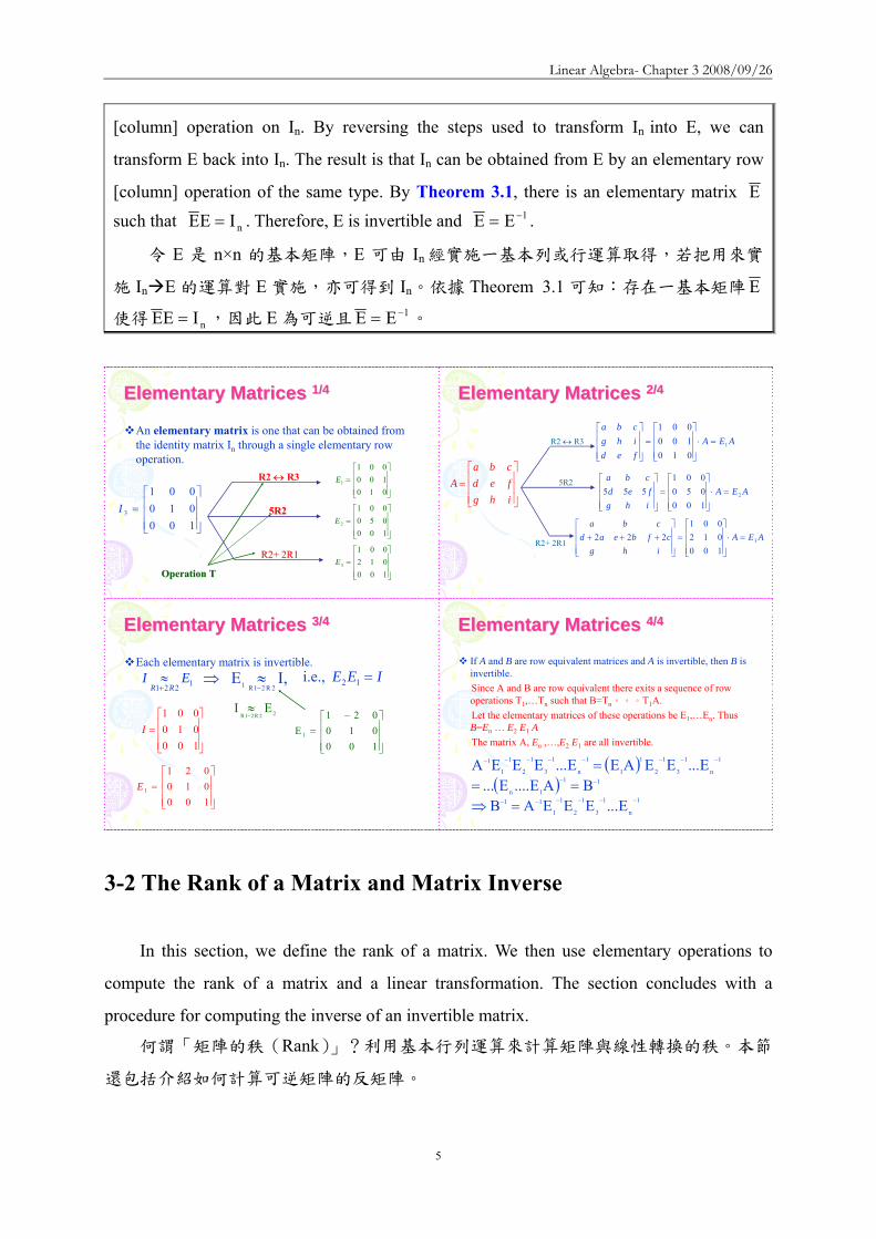
Linear Algebra- Chapter 3 20080926
5
[column] operation on In By reversing the steps used to transform In into E we can
transform E back into In The result is that In can be obtained from E by an elementary row
[column] operation of the same type By Theorem 31 there is an elementary matrix E
such that nIEE = Therefore E is invertible and 1EE minus=
令 E 是 ntimesn 的基本矩陣E 可由 In 經實施一基本列或行運算取得若把用來實
施 In E 的運算對 E 實施亦可得到 In依據 Theorem 31 可知存在一基本矩陣E
使得 nIEE = 因此 E 為可逆且 1EE minus=
Elementary Matrices Elementary Matrices 1414
An elementary matrix is one that can be obtained from the identity matrix In through a single elementary row operation
⎥⎥⎥
⎦
⎤
⎢⎢⎢
⎣
⎡=
100010001
3I⎥⎥⎥
⎦
⎤
⎢⎢⎢
⎣
⎡=
010100001
1ER2 harr R3
⎥⎥⎥
⎦
⎤
⎢⎢⎢
⎣
⎡=
100050001
2E5R25R2
⎥⎥⎥
⎦
⎤
⎢⎢⎢
⎣
⎡=
100012001
3ER2+ 2R1R2+ 2R1
Operation TOperation T
Elementary Matrices Elementary Matrices 2424
⎥⎥⎥
⎦
⎤
⎢⎢⎢
⎣
⎡=
ihgfedcba
A
AEAfedihgcba
1
010100001
=sdot⎥⎥⎥
⎦
⎤
⎢⎢⎢
⎣
⎡=
⎥⎥⎥
⎦
⎤
⎢⎢⎢
⎣
⎡R2 harr R3
AEAihgfed
cba
2
100050001
555 =sdot⎥⎥⎥
⎦
⎤
⎢⎢⎢
⎣
⎡=
⎥⎥⎥
⎦
⎤
⎢⎢⎢
⎣
⎡5R2
AEAihg
cfbeadcba
3
100012001
222 =sdot⎥⎥⎥
⎦
⎤
⎢⎢⎢
⎣
⎡=
⎥⎥⎥
⎦
⎤
⎢⎢⎢
⎣
⎡+++
R2+ 2R1
Elementary Matrices Elementary Matrices 3434
Each elementary matrix is invertible
1221EI
RR +asymp
⎥⎥⎥
⎦
⎤
⎢⎢⎢
⎣
⎡=
100010021
1E
⎥⎥⎥
⎦
⎤
⎢⎢⎢
⎣
⎡=
100010001
I
IE 2R21R1 minus
asymprArr IEE =12 ie
22R21REI
minusasymp
⎥⎥⎥
⎦
⎤
⎢⎢⎢
⎣
⎡ minus=
100010021
E 1
Elementary Matrices Elementary Matrices 4444
If A and B are row equivalent matrices and A is invertible then B is invertibleSince A and B are row equivalent there exits a sequence of row operations T1hellipTn such that B=TnT1ALet the elementary matrices of these operations be E1hellipEn Thus B=En hellip E2 E1 AThe matrix A En hellipE2 E1 are all invertible
( )( )
1
n
1
3
1
2
1
111
11
1n
1
n
1
3
1
2
1
1
1
n
1
3
1
2
1
11
EEEEABBAEE
EEEAEEEEEA
minusminusminusminusminusminus
minusminus
minusminusminusminusminusminusminusminus
=rArr==
=
3-2 The Rank of a Matrix and Matrix Inverse
In this section we define the rank of a matrix We then use elementary operations to
compute the rank of a matrix and a linear transformation The section concludes with a
procedure for computing the inverse of an invertible matrix
何謂「矩陣的秩(Rank)」利用基本行列運算來計算矩陣與線性轉換的秩本節
還包括介紹如何計算可逆矩陣的反矩陣
Linear Algebra- Chapter 3 20080926
6
DEFINITION 33 Rank of a Matrix
If AisinMmtimesn(F) we define the rank of A denoted rank(A) to be the rank of the linear
transformation LA Fn Fm
若 AisinMmtimesn(F)則矩陣 A 的秩為線性轉換 LA Fn Fm的秩註記為 rank(A)
An ntimesn matrix is invertible if and only if its rank is n
一個 ntimesn 的矩陣為可逆的『若且唯若』條件為該矩陣的 Rank 為 n
Every matrix A is the matrix representation of the linear transformation LA with respect
to the appropriate standard ordered bases Thus the rank of the linear transformation LA is the
same as the rank of one of its matrix representation namely A
每一個矩陣 A 是線性轉換 LA 對於某個標準有序基底的矩陣表示式因此該線性轉
換 LA的 Rank 就等於矩陣表示式 A 的 Rank即 rank(LA) = rank(A)
DEFINITION 29
Let V and W be vector spaces and let T V W be linear If N(T) and R(T) are finite-
dimensional then we define the nullity of T denoted nullity(T) and the rank of T denoted
rank(T) to be the dimensions of N(T) and R(T) respectively
V 與 W 為向量空間且 T V W 為線性轉換
定義 T 的核次數(Nullity)nullity(T) = dimensions of N(T)
定義 T 的秩(Rank)rank(T) = dimension of R(T)
核次數(Nullity)與秩(Rank)分別代表 N(T)與 R(T)的維度
DEFINITION 211
Let β = u1 u2hellip un be an ordered basis for a finite-dimensional vectors space V
For xisinV let a1 a2hellip an be the unique scalars such that
令 β = u1 u2hellip un為有限向量空間 V 的有序基底則存在唯一的一組純量 a1
a2hellip an使得 V 內任意向量均可表達成該組基底的線性組合
sum=
=n
1iiiuax
we define the coordinate vector of x relative to β denoted β[x] by
Linear Algebra- Chapter 3 20080926
7
⎟⎟⎟⎟⎟
⎠
⎞
⎜⎜⎜⎜⎜
⎝
⎛
=β
n
2
1
a
aa
[x] 稱為 x 相對於有序基底 β的座標向量
DEFINITION 212
Suppose that V and W are finite-dimensional vector spaces with ordered bases β = v1
v2hellip vn and γ = w1 w2hellip wn respectively Let T V W be linear Then for each j 1
≦j≦n there exist unique scalars aijisinF 1≦i≦m such that
sum==
m
1iiijj wa)vT( for 1≦j≦n
We call the mtimesn matrix A defined by Aij = aij the matrix representation of T in the ordered bases β and γ and write γ
β= [T]A
If V = W and β = γ then we write β= [T]A
設 V 與 W 分別為有限維度的向量空間β = v1 v2hellip vn與 γ = w1 w2hellip
wn分別為 V 與 W 的有序基底且 T V W 為 V 映至 W 的線性轉換
對每一個 j(1≦ j≦n)而言存在唯一的純量 aij isinF(1≦ i≦m)使得
sum==
m
1iiijj wa)vT(
將 mtimesn 的矩陣 A 定義為 Aij = aij並稱呼 A 為線性轉換 T 的矩陣表達方式在
V 與 W 分別以 β 與 γ作為有序基底下A 可註記為 γβ= [T]A
若 V = W 且 β = γ則 β= [T]A
提示 sum==
m
1iiijj wa)vT( 為「將 vj的像 T(vj)表達成有序基底 γ的線性組合」
DEFINITION 217
Let A be an mtimesn matrix with entries from a field F We denote by LA the mapping LA
Fn Fm defined by LA(x) = Ax (the matrix product A and x) for each column vector xisinFn
We call LA a left-multiplication transformation
令 A 是 mtimesn 的矩陣所有元素均來自 FLA為 Fn映至 Fm的線性轉換並定義為
LA(x) = Ax其中 x 為行向量(Column vector)且 xisinFnLA被稱為左乘法轉換
Linear Algebra- Chapter 3 20080926
8
The next theorem extends this fact to any matrix representation of any linear
transformation defined on finite-dimensional vector spaces
Theorem 33 Let T V W be a linear transformation between finite dimensional vector spaces and
let β and γ be ordered bases for V and W respective Then rank(T) = rank( γβ[T] )
令 T V W且 β 與 γ 分別為有限維度向量空間 V 與 W 的有序基底則
rank(T) = rank( γβ[T] )
改寫 Definition 212
Suppose that Fn and Fm are finite-dimensional vector spaces with ordered bases β =
v1 v2hellip vn and γ = w1 w2hellip wn respectively Let LA Fn Fm be linear and defined
by LA(x) = Ax Then for each j 1≦j≦n there exist unique scalars aijisinF 1≦i≦m such
that sum=
=m
1iiijjA wa)v(L for 1≦j≦n We call the mtimesn matrix A defined by Aij = aij the matrix
representation of LA in the ordered bases β and γ and write γβ= ][LA A
Now that the problem of finding the rank of a linear transformation has been reduced to
the problem of finding the rank of a matrix we need a result that allows us to perform rank-
preserving operations on matrices The next theorem and its corollary tell us how to do this
線性轉換的 Rank 可以被簡化為找矩陣的 Rank如何找矩陣的 Rank
Theorem 34 Let A be an mtimesn matrix If P and Q are invertible mtimesm and ntimesn matrices respectively
then
令 A 為 mtimesn 的矩陣若 P 與 Q 分別為可逆的 mtimesm 與 ntimesn 矩陣則
(a) rank(AQ) = rank(A)
(b) rank(PA) = rank(A)
(c) rank(PAQ) = rank(A)
【Proof】
R(LAQ) = R(LALQ) = LALQ(Fn) = LA(LQ(Fn)) = LA(Fn) = R(LA)
Since LQ is onto rank(AQ) = dim(R(LAQ)) = dim(R(LA)) = rank(A)
Linear Algebra- Chapter 3 20080926
9
rank(PAQ) = rank(PA) = rank(A)
註Theorem 34 是為後續 Reduced Row Echelon Form of Matrix 做準備一個矩陣經過
基本行運算或基本列運算或基本行與列運算後並不會改變 RANK
Corollary
Elementary row and column operations on a matrix are rank-preserving
矩陣的基本列與行運算不會改變矩陣的 Rank
此推論結果是計算反矩陣解線性方程組的重要依據
Theorem 35 The rank of any matrix equals the maximum number of its linearly independent
columns that is the rank of a matrix is the dimension of the subspace generated by its
column
任一矩陣的 Rank 等於其最大線性獨立行向量數目即矩陣的 Rank 是由矩陣的
行向量生成的子空間的維度【LA Fn Fm】
【Proof】
For any AisinMmtimesn(F)
rank(A) = rank(LA) = dim(R(LA))
Let β be the standard basis of Fn Then β spans Fn and hence by Theorem 22
R(LA ) = span(LA (β)) = span(LA(e1) LA(e2)hellip LA(en))
But for any j we have seen in Theorem 213(b) that LA(ej) = Aej = aj where aj is the
jth column of A Hence R(LA ) = span(a1 a2 an)
Thus rank(A) = rank(LA) = dim(span(a1 a2 an))
對任意矩陣 Arank(A) = rank(LA) = dim(R(LA))
令 β為 Fn 的標準基底且生成 Fn
依據 Theorem 22
LA的值域 Range 可由 LA(β)來生成
R(LA) = span(LA (β)) = span(LA(e1) LA(e2)hellip LA(en))
對任意 j 而言由 Theorem 213(b) 可知 LA(ej) = Aej = aj其中aj 為 A 的第 j
個行(aj 相當於 Theorem 213(b)的 vj 或 Theorem 22 的 T(vj))因此 R(LA) =
Linear Algebra- Chapter 3 20080926
10
span(a1 a2 an)
所以 rank(A) = rank(LA) = dimension of R(LA) = dim(span(a1a2an))
Theorem 22 令 V 與 W 為向量空間且 T V W 為線性轉換若 β = v1 v2hellip vn
是定義域(Domain)V 的基底則 T 的值域 Range R(T)可由 T(β)來生成意即 R(T)
= span(T(β)) = span(T(v1) T(v2)hellip T(vn))
Theorem 213 A 為 mtimesn 的矩陣與 B 為 ntimesp 的矩陣uj 與 vj分別為 AB 與 B 的第 j 行
(1 j p≦ ≦ )則
(a) uj = A vj
(b) vj = B ej where ej is the jth standard vector of Fp
EXAMPLE 1
Let ⎟⎟⎟
⎠
⎞
⎜⎜⎜
⎝
⎛=
101110101
A
Observe that the first and second columns of A are linearly independent and that the
third column is a linear combination of the first two Thus
A 的第一行與第二行是線性獨立第三行則是前兩行的線性組合於是
rank(A) = dim⎟⎟⎟⎟
⎠
⎞
⎜⎜⎜⎜
⎝
⎛
⎟⎟⎟
⎠
⎞
⎜⎜⎜
⎝
⎛
⎪⎭
⎪⎬
⎫
⎟⎟⎟
⎠
⎞
⎜⎜⎜
⎝
⎛
⎪⎩
⎪⎨
⎧
⎟⎟⎟
⎠
⎞
⎜⎜⎜
⎝
⎛
⎟⎟⎟
⎠
⎞
⎜⎜⎜
⎝
⎛
111
010
101
span = 2
A 的第 1 行a1=⎟⎟⎟
⎠
⎞
⎜⎜⎜
⎝
⎛
101第 2 行a2=
⎟⎟⎟
⎠
⎞
⎜⎜⎜
⎝
⎛
010第 3 行a3=
⎟⎟⎟
⎠
⎞
⎜⎜⎜
⎝
⎛
111
In order to compute the rank of a matrix A it is frequently useful to postpone the use of
Theorem 35 until A has been suitable modified by means of appropriate elementary row and
column operations so that the number of linearly independent columns is obvious
為了利用 Theorem 35 求矩陣 A 的 Rank(等於最大線性獨立行向量數目)A 可
先經過基本列或行運算使其線性獨立的行數變得比較明顯
EXAMPLE 2 Let
Linear Algebra- Chapter 3 20080926
11
⎟⎟⎟
⎠
⎞
⎜⎜⎜
⎝
⎛=
211301121
A
If we subtract the first row of A from rows 2 and 3 (type 3 elementary row operations)
the result is
⎟⎟⎟
⎠
⎞
⎜⎜⎜
⎝
⎛
minusminus
110220121
If we now substract twice the first column from the second and substract the first
column from the third (type 3 elementary column operations) we obtain
⎟⎟⎟
⎠
⎞
⎜⎜⎜
⎝
⎛
minusminus
110220001
(後二行線性相依最大線性獨立行數為 2)
It is now obvious that the maximum number of linearly independent column of this matrix is 2 Hence the rank of A is 2
Theorem 36 Let A be an mtimesn matrix of rank r Then r m r n and by means of a finite number ≦ ≦
of elementary row and column operations A can be transformed into the matrix
D = ⎟⎟⎠
⎞⎜⎜⎝
⎛
32
1r
OOOI
where O1 O2 and O3 are zero matrices Thus Dii = 1 for i r and ≦
Dij = 0 otherwise
令 A 為 Rank 等於 r 的 mtimesn 矩陣則 r m≦ 且 r n≦ 經過有限次數的基本行與列
運算讓 A 化成 D = ⎟⎟⎠
⎞⎜⎜⎝
⎛
32
1r
OOOI
其中Ir 為對角元素為 1 的對角矩陣即 A 可經
過有限次數的基本行及列運算取得沿對角線前 r 個位置皆為 1其餘各處皆為 0 的
矩陣 D
【Proof】
If A is the zero matrix r = 0 In this case the conclusion follows with D = A
若 A 為零矩陣則 r = 0 且 D = A
Now suppose that AneO and r = rank(A) then r gt 0
The proof is by mathematical induction on m the number of rows of A
若 A 非零矩陣且 r = rank(A)則 r gt 0
Linear Algebra- Chapter 3 20080926
12
採用數學歸納法
Suppose that m = 1
A can be transformed into the matrix (1 0 hellip0)
So rank(D) = rank(A) = 1 by Corollary to Theorem 34 and Theorem 35 Thus the
theorem is established for m = 1
設 m = 1則 A 可以化成(1 0 hellip0)
依據 Corollary to Theorem 34 及 Theorem 35
rank(D) = rank(A) = 1
故本定理對 m = 1 的矩陣是成立的
Next assume that the theorem holds for any matrix with at most m - 1 row (for some m
gt1)
We must prove that the theorem holds for any matrix with m rows
其次假設本定理對至多含 m - 1 列的矩陣皆成立(m gt 1)
至於含 m 列的矩陣是否成立
If n = 1 Theorem 36 can be established in a manner analogous to that for m = 1
若 n = 1則可按 m = 1 的方式證明本定理對於 n = 1 的矩陣成立
We now suppose that n gt 1 Since A ne O Aijne0 for some i j By means of at most one
elementary row and at most one elementary column operation (each of type 1) We can
move the nonzero entry to the 11 position By means of of at most one additional type 2
operation we can assure a 1 in the 11 position By means of at most m ndash 1 type 3 row
operations and at most n ndash 1 type 3 column operations we can eliminate all nonzero entries
in the first row and the first column with the exception of the 1 in the 11 postion
Thus with a finite number of elementary operation A can be transformed into a
matrix
經過有限次數的基本行及列運算可將 A 轉換成
⎪⎪⎭
⎪⎪⎬
⎫
⎪⎪⎩
⎪⎪⎨
⎧
=
0B
0001
B where Brsquo is an (m-1)times(n-1) matrix
Brsquo has rank one less than B
Brsquo的 Rank 比 B 少 1
Since rank(A) = rank(B) = r rank(Brsquo) = r ndash 1 Therefore r ndash1 ≦ m ndash 1 and r ndash1 ≦
Linear Algebra- Chapter 3 20080926
13
n ndash 1 by the induction hypothesis Hence r ≦ m and r ≦ n
由於 rank(A) = rank(B) = r故 rank(Brsquo) = r ndash 1
依數學歸納法 r ndash1 ≦ m ndash 1 且 r ndash1 ≦ n ndash 1
因此 r ≦ m 且 r ≦ n
Also by the induction hypothesis Brsquo can be transformed by a finite number of
elementary row and column operations into the (m-1)times(n-1) matrix Drsquo such that
同樣地依據數學歸納法Brsquo 可經過有限次數的基本行與列運算轉換成 (m-
1)times(n-1) 的矩陣 Drsquo使得
Dlsquo= ⎟⎟⎠
⎞⎜⎜⎝
⎛ minus
65
41r
OOOI
where O4 O5 and O6 are zero matrices
That is Drsquo consists of all zeros except for its first r-1 diagonal entries which are ones
Let
⎪⎪⎭
⎪⎪⎬
⎫
⎪⎪⎩
⎪⎪⎨
⎧
=
0D
0001
D
We see that the theorem now follows once we show that D can be obtained from B by
means of a finite number of elementary row and column operations
D 可由 B 經過有限次基本行及列運算而取得
Thus since A can be transformed into B and B can be transformed into D each by a
finite number of elementary operations A can be transformed into D by a finite number of
elementary operations
經過有限次基本行及列運算A B D
Finally since Drsquo contains ones as its first r ndash 1 diagonal entries D contains ones as its
first r diagonal entries and zeros elsewhere
最後Drsquo沿對角線前 r-1 個位置皆為 1故 D 沿對角線前 r 個位置皆為 1其餘
各處皆為 0
EXAMPLE 3 Consider the maxtrix
⎟⎟⎟⎟⎟
⎠
⎞
⎜⎜⎜⎜⎜
⎝
⎛
=
192362100280844422420
A
Linear Algebra- Chapter 3 20080926
14
By means of a succession of elementary row and column operations we can transform
A into a matrix D as in Theorem 36
透過一系列的基本行與列運算將 A 轉換成 D
D
00000001000001000001
192362100280844422420
A =
⎟⎟⎟⎟⎟
⎠
⎞
⎜⎜⎜⎜⎜
⎝
⎛
==
⎟⎟⎟⎟⎟
⎠
⎞
⎜⎜⎜⎜⎜
⎝
⎛
=
By the corollary to Theorem 34 rank(A) = rank(D) Clearly however rank(D) = 3 so rank(A) = 3
Corollary 1 Let A be an mtimesn matrix of rank r Then there exist invertible matrices B and C of sizes
mtimesm and ntimesn respectively such that D = BAC where D = ⎟⎟⎠
⎞⎜⎜⎝
⎛
32
1r
OOOI
is the mtimesn matrix
in which O1 O2 and O3 are zero matrices
令 A 為 mtimesn 的矩陣Rank 為 r存在可逆的 mtimesm 矩陣 B 與 ntimesn 矩陣 C使得
D = BAC其中D = ⎟⎟⎠
⎞⎜⎜⎝
⎛
32
1r
OOOI
為 mtimesn 的矩陣O1O2 及 O3 為零矩陣
【Proof】
By Theorem 36 A can be transformed by means of a finite number of elementary
row and column operations into the matrix D
We can appeal to Theorem 31 each time we perform an elementary operation Thus
there exist elementary mtimesm matrices E1 E2hellipEp and elementary ntimesn matrices G1
G2hellipGq such that D = EpEp-1hellipE2E1AG1G2hellipGq
By Theorem 32 each Ej and Gj is invertible Let B = EpEp-1hellipE2E1 and C =
G1G2hellipGq Then B and C are invertible and D = BAC
依據 Theorem 36A 可經過有限次的基本列與行運算化成 D
引用 Theorem 31每一次皆實施某一個基本列運算於是存在基本的 mtimesm 矩
陣 E1 E2hellip Ep 與 基 本 的 ntimesn 矩 陣 G1 G2hellip Gq 使 得 D = EpEp-
1hellipE2E1AG1G2hellipGq
依據 Theorem 32 每一個基本矩陣 Ej與 Gj 皆為可逆令 B = EpEp-1hellipE2E1 與 C =
G1G2hellipGq於是 B 與 C 皆為可逆且 D = EpEp-1hellipE2E1AG1G2hellipGq = BAC
Linear Algebra- Chapter 3 20080926
15
Theorem 31 令 AisinMmtimesn(F)並假設 B 是由 A 經實施某一基本列【或行】運算後所得
到的矩陣則存在一個 mtimesm 【或 ntimesn】基本矩陣 E使得 B = EA【或 B = AE】E
矩陣是由 Im 【或 In】 經實施與「由 A 得到 B」相同的基本列【或行】運算後所得
到的矩陣反之若 E 是一個 mtimesm【或 ntimesn】的基本矩陣則 EA【或 AE】是由 A
經過與「由 Im 【或 In】 得到 E」相同的基本列【或行】運算後所得到的矩陣
Theorem 32 基本矩陣為可逆矩陣且基本矩陣的反矩陣亦是同一型的基本矩陣
Theorem 36 令 A 為 Rank 等於 r 的 mtimesn 矩陣則 r m≦ 且 r n≦ 經過有限次數的基
本行與列運算讓 A 化成 D = ⎟⎟⎠
⎞⎜⎜⎝
⎛
32
1r
OOOI
其中Ir為對角元素為 1 的對角矩陣
Corollary 2 Let A be an mtimesn matrix Then
(a) rank(At) = rank(A)
矩陣轉置後的 RANK 不變
(b) The rank of any matrix equals the maximum number of its linearly independent
rows that is the rank of a matrix is the dimension of the subspace generated by
rows
任一矩陣的 Rank 等於最大線性獨立列向量的數目即矩陣的 Rank 等於由該
矩陣列向量所生成的子空間的維度
(c) The rows and columns of any matrix generate subspaces of the same dimension
numerically equal to the rank of the matrix
任一矩陣的列向量與行向量生成的子空間的維度相同維度等於該矩陣的
Rank
【Proof】
By Corollary 1 there exist invertible matrices B and C such that D = BAC where D
satisfies the stated conditions of the corollary Taking transposes we have
Dt = (BAC) t = CtAtBt
Since B and C are invertible so are Bt and Ct
Hence by Theorem 34 rank(At) = rank(CtAtBt) = rank(Dt)
Suppose that r = rank(A)
Then Dt is an ntimesm matrix with the form of the matrix D in Corollary 1 and hence
Linear Algebra- Chapter 3 20080926
16
rank(Dt) = r by Theorem 35
Thus
rank(At) = rank(Dt) = r = rank(A)
依據 Corollary 1存在可逆矩陣 B 與 C使得 D = BAC
取其轉置可得Dt = (BAC) t = CtAtBt
由於 B 與 C 為可逆故 Bt 與 Ct 亦為可逆
依據 Theorem 34得知 rank(At) = rank(CtAtBt) = rank(Dt)
設 r = rank(A)
則 Dt為一 ntimesm 的矩陣型式與 D 相同(參考 Corollary 1)
且依據 Theorem 35 得知 rank(Dt) = r
於是 rank(At) = rank(Dt) = r = rank(A)
Theorem 34 Let A be an mtimesn matrix If P and Q are invertible mtimesm and ntimesn matrices
respectively then 令 A 為 mtimesn 的矩陣若 P 與 Q 分別為可逆的 mtimesm 與 ntimesn 矩陣
則
(a) rank(AQ) = rank(A)
(b) rank(PA) = rank(A)
(c) rank(PAQ) = rank(A)
Theorem 35 The rank of any matrix equals the maximum number of its linearly
independent columns that is the rank of a matrix is the dimension of the subspace
generated by its column 任一矩陣的 Rank 等於其最大線性獨立行向量數目即矩陣
的 Rank 是由矩陣的行向量生成的子空間的維度【LA Fn Fm】
Corollary 3 Every invertible matrix is a product of elementary matrices
每一可逆矩陣均可為基本矩陣的乘積
【Proof】
If A is an invertible ntimesn matrix then rank(A) = n Hence the matrix D in Corollary 1
equals In and there exist invertible matrices B and C such that In = BAC
As in the proof of Corollary 1 note that B = EpEp-1hellipE2E1 and C = G1G2hellipGq where
the Eirsquos and Girsquos are elementary matrices Thus A = B-1InC-1 = B-1C-1 so that
A = E1-1E2
-1hellipEp-1Gq
-1Gq-1-1hellipG1
-1
Linear Algebra- Chapter 3 20080926
17
The inverses of elementary matrices are elementary matrices however and hence A is
the product of elementary matrices
若 A 為可逆的 ntimesn 矩陣則 rank(A) = n
因此 Corollary 1 中的矩陣 D 為 In且存在可逆的 B 與 C 矩陣使得 In = BAC
如同 Corollary 1 的證明一樣B = EpEp-1hellipE2E1 且 C = G1G2hellipGq其中Eirsquos 與
Girsquos 皆為基本矩陣
於是A = B-1InC-1 = B-1C-1即 A = E1-1E2
-1hellipEp-1Gq
-1Gq-1-1hellipG1
-1
基本矩陣的反矩陣亦為基本矩陣A 是基本矩陣的乘積
Theorem 37 Let T V W and U W Z be linear transformations on finite-dimensional vector
spaces V W and Z and let A and B be matrices such that the product AB is defined Then
令 VW 與 Z 為有限維度的向量空間T V W 與 U W Z 為線性轉換且
A 與 B 為滿足乘積 AB 定義的矩陣則
(a) rank(UT) ≦ rank(U)
(b) rank(UT) ≦ rank(T)
(c) rank(AB) ≦ rank(A)
(d) rank(AB) ≦ rank(B)
【Proof】
(a) Clearly R(T)subeW
Hence R(UT) = UT(V) = U(R(T)) sube U(W) = R(U)
Thus rank(UT) = dim(R(UT)) ≦ dim (R(U)) = rank(U)
(c) By (a) rank(AB) = rank(LAB) = rank (LALB) ≦ rank(LA) = rank(A)
(d) By (c) and Corollary 2 to Theorem 36
rank(AB) = rank((AB)t) = rank(B t A t) ≦ rank(B t) = rank (B) (b) Let α β and γ be ordered bases for V W and Z respectively and let Arsquo = γ
β]U[
and Brsquo = βα]T[ Then ArsquoBrsquo = γ
α]UT[ by Theorem 211
Hence by Theorem 33 and (d)
rank(UT) = rank(ArsquoBrsquo) ≦ rank(Brsquo) = rank (T)
Theorem 211 Let V W and Z be finite-dimensional vector space with ordered bases α β
and γ respectively Let T V W and U W Z be linear transformation Then
Linear Algebra- Chapter 3 20080926
18
βα
γβ
γα = [T][U][UT] 令 VW 與 Z 是有限維度的向量空間αβ 與 γ 分別為 VW 與
Z 的有序基底令 T V W (先 α β) 且 U W Z (後 β γ)則 βα
γβ
γα = [T][U][UT]
Theorem 33 Let T V W be a linear transformation between finite dimensional vector
spaces and let β and γ be ordered bases for V and W respective Then rank(T) = rank( γ
β[T] ) 令 T V W且 β 與 γ 分別為有限維度向量空間 V 與 W 的有序基底
則 rank(T) = rank( γβ[T] )
EXAMPLE 4
(a) Let ⎟⎟⎠
⎞⎜⎜⎝
⎛minus
=11111121
A (第一列與第二列是 LI) rank(A) = 2
(b) Let ⎟⎟⎟
⎠
⎞
⎜⎜⎜
⎝
⎛=
003011011131
A (第三列與第一二列是 LD)rank(A) = 2
(c) Let ⎟⎟⎟
⎠
⎞
⎜⎜⎜
⎝
⎛
minus=
011111121321
A (三列為 LI) rank(A) = 3
The inverse of a Matrix
We have remarked that an ntimesn matrix is invertible if and only if its rank is n Since we
know how to compute the rank of any matrix we can always test a matrix to determine
whether it is invertible We now provide a simple technique for computing the inverse of a
matrix that utilizes elementary row operations
已知 ntimesn 矩陣為可逆的『若且唯若』條件為該矩陣的 Rank 等於 n
DEFINITION 34 Augmented Matrix Let A and B be mtimesn and mtimesp matrices respectively By the augmented matrix )BA(
we mean that the mtimes(n+p) matrix )BA( that is the matrix whose first n columns are the
columns of A and whose last p columns are the columns of B 設 A 與 B 分別為 mtimesn 與 mtimesp 的矩陣則增廣矩陣(Augmented matrix) )BA(
Linear Algebra- Chapter 3 20080926
19
為一 mtimes(n+p)的矩陣 )BA( 該矩陣的前 n 行(Column)為 A 的所有的行後 p
行為 B 的所有行
Let A be an invertible ntimesn matrix and consider the ntimes2n augmented matrix C= )IA( n
C= )IA( n )AI()IAAA(CA 1
nn111 minusminusminusminus ==
By Corollary 3 to Theorem 36 A-1 is the product of elementary matrices say
A = EpEp-1hellipE2E1 (A-1 是多個基本矩陣的乘積)
Thus )AI()IAAA(CA 1
nn111 minusminusminusminus == )AI(CA)IA(EEE 1
n1
n11ppminusminus
minus ==
We have the following result If A is an invertible invertible ntimesn matrix then it is
possible to transform the matrix (AIn) into the matrix (InA-1) by means of a finite
number of elementary row operations
若 A 為一可逆的 ntimesn 矩陣則可經過有限次數的基本列運算將矩陣 (AIn) 化成
(InA-1)
Conversely suppose that A is invertible and that for some ntimesn matrix B the matrix
(AIn) can be transformed into the matrix (InB) by a finite number of elementary row
operations Let E1 E2hellip Ep be the elementary matrices associated with these elementary row
operations as in Theorem 31 then
反之假設 A 是可逆且矩陣(AIn)可經有限次數的基本列運算轉換成矩陣(InB)
並令 E1 E2hellip Ep 分別為 Theorem 31 所稱的基本矩陣則
)BI()IA(EEE nn11pp =minus
Let M = EpEp-1hellipE2E1 we have 令 M = EpEp-1hellipE2E1
)BI()IA(EEE nn11pp =minus )BI()IA(M)MMA( nn ==
Linear Algebra- Chapter 3 20080926
20
Hence MA = In and M = B It follows that M = A-1 So B = A-1
可由 MA = In 及 M = B 得知M 就是 A-1故 B 就是 A-1
Thus we have the follow resultsIf A is an invertible ntimesn matrix and the matrix
(AIn) is transformed in a matrix of the form (InB) by means of a finite number of
elementary row operations then B=A-1
若 A 為一可逆的 ntimesn 矩陣且矩陣 (AIn) 可經有限次數的基本列運算化成
(InB)則 B=A-1
If on the other hand A is an ntimesn matrix that is not invertible then rank(A) lt n Hence
any attempt to transform (AIn) into a matrix of the form (InB) by means of elementary row
operations must fail
反之若 A 是一不可逆的 ntimesn 矩陣則 rank(A) lt n因此任何想利用基本列運算
要將矩陣 (AIn) 化成 (InB)的努力必定失敗
Thus we have the follow results If A is an notinvertible ntimesn matrix then any attempt
to transform (AIn) into a matrix of the form (InB) produce a row whose first n entries
are zeros
若 A 是一不可逆的 ntimesn 矩陣任何想將矩陣 (AIn) 化成 (InB)的努力最後會
產生一前 n 個元素均為 0 的列
EXAMPLE 5
We determine whether the matrix ⎟⎟⎟
⎠
⎞
⎜⎜⎜
⎝
⎛=
133242420
A is invertible and if it is we
compute its inverse
A 是否為可逆矩陣
We attempt to use elementary row operations to transfer
Linear Algebra- Chapter 3 20080926
21
⎟⎟⎟
⎠
⎞
⎜⎜⎜
⎝
⎛=
100010001
133242420
)IA( into a matrix of the form (InB)
看看能否利用基本行與列運算將矩陣 (AIn) 化成 (InB)
Interchanging rows 1 and 2
⎟⎟⎟
⎠
⎞
⎜⎜⎜
⎝
⎛
100001010
133420242
Multiplying the first row by 12
⎟⎟⎟
⎠
⎞
⎜⎜⎜
⎝
⎛
10000100
133420121 2
1
Adding -3 times row 1 to row 3
⎟⎟⎟
⎠
⎞
⎜⎜⎜
⎝
⎛
minusminusminus 1000100
230420121
23
21
Multiplying row 2 by 12 to obtain 1 in the 22 position
⎟⎟⎟
⎠
⎞
⎜⎜⎜
⎝
⎛
minus
minus
minusminus 100000
230210121
23
21
21
Adding -2 times row 2 to row 1 and 3 times row 2 to row 3
⎟⎟⎟
⎠
⎞
⎜⎜⎜
⎝
⎛
minus
minusminus
10001
400210301
23
2321
21
Multiplying row 3 by 14
⎟⎟⎟
⎠
⎞
⎜⎜⎜
⎝
⎛
minus
minusminus
41
83
8321
21
0001
100210301
Adding appropriate multiply of row 3 to row 1 and 2 completes the process
⎟⎟⎟
⎠
⎞
⎜⎜⎜
⎝
⎛
minusminus
minus
41
83
83
21
43
41
43
85
81
100010001
目標達成
Thus A is invertible and ⎟⎟⎟
⎠
⎞
⎜⎜⎜
⎝
⎛
+minus+minus+minus+minus+
=minus
41
83
83
21
43
41
43
85
81
1A
Linear Algebra- Chapter 3 20080926
22
EXAMPLE 6
We determine whether the matrix ⎟⎟⎟
⎠
⎞
⎜⎜⎜
⎝
⎛minus=451112
121A is invertible and if it is we
compute its inverse
A 是否為可逆矩陣
We attempt to use elementary row operations to transfer
⎟⎟⎟
⎠
⎞
⎜⎜⎜
⎝
⎛minus=
100010001
451112
121)IA( into a matrix of the form (InB)
看看能否利用基本行與列運算將矩陣 (AIn) 化成 (InB)
Adding -2 times row 1 to row 2 and -1 times row 1 to row 3 then addig row 2 to row
3
⎟⎟⎟
⎠
⎞
⎜⎜⎜
⎝
⎛minus
100010001
451112
121
⎟⎟⎟
⎠
⎞
⎜⎜⎜
⎝
⎛
minusminusminusminus
101012001
330330
121
⎟⎟⎟
⎠
⎞
⎜⎜⎜
⎝
⎛
minusminusminusminus
113012001
000330
121
is a matrix with row whose first 3 entries are zeros Therefore A is not invertible
最後一列前 3 個元素均為 0
EXAMPLE 7 Let T P2(R) P2(R) be defined by T(f(x)) = f(x)+frsquo(x)+frdquo(x) where frsquo(x) and frdquo(x)
denote the first and second derivatives of f(x) We use Corollary 1 to Theorem 218 to test
T for invertibility and compute the inverse if T is invertible Taking β=1 x x2 to be the
standard ordered basis of P2(R) we have
令 T P2(R) P2(R) 為線性轉換且定義為 T(f(x)) = f(x)+frsquo(x)+frdquo(x)利用
Corollary 1 to Theorem 218 來測試 T 是否可逆並計算其逆轉換取 β=1 x x2為
P2(R)的標準有序基底
T(1) = 1 = 1bull1+0bullx+0bullx2
T(x) = 1+x = 1bull1+1bullx+0bullx2
Linear Algebra- Chapter 3 20080926
23
T(x2) = 2+2x+x2 = 2bull1+2bullx+1bullx2
⎟⎟⎟
⎠
⎞
⎜⎜⎜
⎝
⎛=β
100210211
[T] 稱為 T 相對有序基底 β的座標向量
依據 Corollary 1 to Theorem 218 T 可逆『若且唯若』 β[T] 可逆且
1-1 )[T](][T minusββ =
Using the method of Examples 5 and 6 we can show that β[T] is invertible with
inverse
⎟⎟⎟
⎠
⎞
⎜⎜⎜
⎝
⎛minus
minus=minus
β
100210
011)([T] 1
Thus T is is invertible and βminusminus
β = ][T)([T] 11 Hence by Theorem 214 we have
⎟⎟⎟
⎠
⎞
⎜⎜⎜
⎝
⎛minusminus
=⎟⎟⎟
⎠
⎞
⎜⎜⎜
⎝
⎛
⎟⎟⎟
⎠
⎞
⎜⎜⎜
⎝
⎛minus
minus=++ β
minus
2
21
10
2
1
02
2101
aa2aaa
aaa
100210
011)]xaxa(a[T
Therefore T-1(a0+a1x+a2x2) = (a0-a1)+(a1-2a2)x+a2x2 Corollary 1 to Theorem 218 Let V be finite-dimensional vector space with an ordered basis β and let T V V be linear Then T is invertible if and only if β[T] is invertible
Furthermore 1-1 )[T](][T minusββ = V 為有限維度的向量空間β 是 V 的有序基底令 T
V V 為線性轉換 T 為可逆的『若且唯若』條件為 β[T] 可逆再者
1-1 )[T](][T minusββ =
Theorem 214 Let V and W be finite-dimensional vector spaces having ordered bases β and γ respectively and let T V W be linear Then for each uisinV we have β
γβγ = [u][T][T(u)]
V 與 W 為有限維度的向量空間β 與 γ分別 V 與 W 的有序基底令 T V W 為線
性轉換則 V 中的 u 映至 W 的結果 T(u) 相對於有序基底 γ 的座標向量為
βγβγ = [u][T][T(u)]
Invertible and Inverse of MATRIX Let A be an n times n matrix If a matrix B can be found such that AB = BA = In then A is
Linear Algebra- Chapter 3 20080926
24
said to be invertible and B is called the inverse of A (denote B = A-1 and A-k=(A-1)k )
If such a matrix B does not exist then A has no inverse
EXAMPLE
⎥⎦
⎤⎢⎣
⎡=
4321
A and ⎥⎦
⎤⎢⎣
⎡minus
minus=
21
23
12B
221
23
221
23
I1001
432112
BA
I100112
4321
AB
=⎥⎦
⎤⎢⎣
⎡=⎥
⎦
⎤⎢⎣
⎡⎥⎦
⎤⎢⎣
⎡minus
minus=
=⎥⎦
⎤⎢⎣
⎡=⎥
⎦
⎤⎢⎣
⎡minus
minus⎥⎦
⎤⎢⎣
⎡=
Thus AB = BA = I2 proving that the matrix A has inverse B
Theorem The inverse of an invertible matrix is unique
Let B and C be inverse of A
Thus AB = BA = In and AC = CA = In
Multiply both sides of the equation AB = In by C
C(AB) = CIn (CA)B = C
InB = C B = C
Thus an invertible matrix has only one inverse
How to find AHow to find A--11
Based on the GaussBased on the Gauss--Jordan algorithmJordan algorithmLet A be an invertible matrix Then AALet A be an invertible matrix Then AA--11=I=Inn
Let the columns of Let the columns of AA--11 be be XX11 XX22 helliphellip XXnn and the columns of I and the columns of Inn be be CC11CC22helliphellipCCnn
Find AFind A--11 by finding by finding XX11 XX22 helliphellip XXnn Write the equation AAWrite the equation AA--11=I=Inn in the formin the form
[ ] [ ]n21nn211 CCCI XXXALet LL ==minus
[ ] [ ][ ] [ ]n21n21
n21n21
CCCAXAXXACCCXXXALL
LL
=rArr=
nn2211 CAXCAX CAX === LThus
How to find AHow to find A--11
Solving these systems by using Gauss-Jordan elimination on the large augmented matrix [AC1 C2hellipCn]
Thus when A-1 exits
[ ] [ ] [ ] 1n
1nn ABwhereBIAIIA minusminus ==asympasympL
If the reduced echelon form of [If the reduced echelon form of [AIAInn] is computed and ] is computed and the first part is not of the form Ithe first part is not of the form Inn then A has no inversethen A has no inverse
[ ][ ]n21n
n21
XXXI CCCAmatrix augmented
LL
L
asympasymp
Linear Algebra- Chapter 3 20080926
25
Example Example 1212
⎥⎥⎥
⎦
⎤
⎢⎢⎢
⎣
⎡
minusminusminusminusminus
=100531010532001211
]IA[ 3
⎥⎥⎦
⎤
⎢⎢⎣
⎡minusminusminus
minusminus
+minus+
asymp
101320012110001211
1RR1R3
2)(R2
⎥⎥⎦
⎤
⎢⎢⎣
⎡minus
minusminusminusasymp
101320012110001211
R2)1(
⎥⎥⎥
⎦
⎤
⎢⎢⎢
⎣
⎡
minusminusminusminusminus
=531532211
ADetermine the inverse of
Example Example 2222
⎥⎥⎦
⎤
⎢⎢⎣
⎡
minusminusminusminus
minus++asymp
123100012110013101
R2)2(R3R2R1
⎥⎥⎦
⎤
⎢⎢⎣
⎡
minusminusminus
minus++asymp
123100135010010001
R3)1(R2R3R1
123135110
A 1
⎥⎥⎥
⎦
⎤
⎢⎢⎢
⎣
⎡
minusminusminus=minus
⎥⎥⎦
⎤
⎢⎢⎣
⎡
minusminus
minus
+minus+asymp
135000011210012301
3R2R3R2)1(R1
ExampleExampleDetermine the inverse of
⎥⎥⎦
⎤
⎢⎢⎣
⎡
minus=
412721511
A
⎥⎥⎦
⎤
⎢⎢⎣
⎡
minus=
100412010721001511
][ 3IA
⎥⎥⎦
⎤
⎢⎢⎣
⎡
minusminusminusminus
minus+minus+asymp
102630011210001511
R1)2(R31)R1(R2
There is no need to proceed further There is no need to proceed further The reduced echelon form cannot have a one in the (3 3) locatioThe reduced echelon form cannot have a one in the (3 3) location n
The reduced echelon form cannot be of the form [IThe reduced echelon form cannot be of the form [Inn B] B] Thus Thus AAndashndash11 does not existdoes not exist
Properties of Matrix InverseProperties of Matrix Inverse
Let Let AA and and BB be invertible matrices andbe invertible matrices and cc a nonzero scalar a nonzero scalar ThenThen
AA =minusminus 11)( 111 1)( 2 minusminus = A
ccA
111)( 3 minusminusminus = ABAB
nn AA )()( 4 11 minusminus =tt AA )()( 5 11 minusminus =
Color Models Color Models 1212
A color model in the context of graphics is a method of A color model in the context of graphics is a method of implementing colorsimplementing colorsThe common used models include RGB model and YIQ modelThe common used models include RGB model and YIQ modelThe RGB model is used in computer monitors and the YIQ model The RGB model is used in computer monitors and the YIQ model is used in television screensis used in television screensAn RGB computer signal can be converted to a YIQ television An RGB computer signal can be converted to a YIQ television signal using the matrix transformationsignal using the matrix transformation
⎥⎥⎥
⎦
⎤
⎢⎢⎢
⎣
⎡
⎥⎥⎥
⎦
⎤
⎢⎢⎢
⎣
⎡
minusminusminus=
⎥⎥⎥
⎦
⎤
⎢⎢⎢
⎣
⎡
BGR
311523212321275596
114587299
QIY
YIQgtRGBYIQgtRGB
Color Models Color Models 2222
A signal is converted from a television screen to a computer monA signal is converted from a television screen to a computer monitor itor using inverse of the above matrixusing inverse of the above matrix
⎥⎥⎥
⎦
⎤
⎢⎢⎢
⎣
⎡
⎥⎥⎥
⎦
⎤
⎢⎢⎢
⎣
⎡
minusminusminus=
⎥⎥⎥
⎦
⎤
⎢⎢⎢
⎣
⎡rArr
⎥⎥⎥
⎦
⎤
⎢⎢⎢
⎣
⎡
⎥⎥⎥
⎦
⎤
⎢⎢⎢
⎣
⎡
minusminusminus=
⎥⎥⎥
⎦
⎤
⎢⎢⎢
⎣
⎡minus
QIY
0751108116472721
6209561
BGR
QIY
311523212321275596
114587299
BGR 1
CryptographyCryptography 密碼學密碼學 1212
Cryptography is the process of coding and decoding messagesCryptography is the process of coding and decoding messagesThe technique can be traced back to the ancient Greeks Today The technique can be traced back to the ancient Greeks Today governments use sophisticated methods of coding and decoding governments use sophisticated methods of coding and decoding messagesmessagesOne type of code that is extremely difficult to break makes use One type of code that is extremely difficult to break makes use of a of a large matrix to encode a message large matrix to encode a message The receiver of the message decodes it using the inverse of the The receiver of the message decodes it using the inverse of the matrixmatrixThe first matrix is called the encoding matrix and its inverse The first matrix is called the encoding matrix and its inverse is is called the decoding matrixcalled the decoding matrix
Cryptography Cryptography 密碼學密碼學 2222
A A-1Message
Encoding MatrixEncoding Matrix
Decoded MessageTransmission
Decoding MatrixDecoding Matrix
Linear Algebra- Chapter 3 20080926
26
Example Example 1212
Let the message be Let the message be BUY IBM STOCKBUY IBM STOCKAnd the encoding matrix beAnd the encoding matrix be
⎥⎥⎥
⎦
⎤
⎢⎢⎢
⎣
⎡ minusminusminus
434110433
B U Y B U Y -- I B M I B M -- S T O C KS T O C K2 21 25 27 9 2 13 27 19 20 15 3 112 21 25 27 9 2 13 27 19 20 15 3 11
⎥⎥⎥
⎦
⎤
⎢⎢⎢
⎣
⎡ minusminusminusminusminus=
⎥⎥⎥
⎦
⎤
⎢⎢⎢
⎣
⎡
⎥⎥⎥
⎦
⎤
⎢⎢⎢
⎣
⎡ minusminusminus
2331372091431715418461146
222117196116169
27319225271527921112013272
434110433
EncodingEncoding
Example Example 2222
Let the message be Let the message be BUY IBM STOCKBUY IBM STOCKAnd the decoding matrix beAnd the decoding matrix be
⎥⎥⎥
⎦
⎤
⎢⎢⎢
⎣
⎡
minusminus 334344101
B U Y B U Y -- I B M I B M -- S T O C KS T O C K2 21 25 27 9 2 13 27 19 20 15 3 112 21 25 27 9 2 13 27 19 20 15 3 11
⎥⎥⎥
⎦
⎤
⎢⎢⎢
⎣
⎡=
⎥⎥⎥
⎦
⎤
⎢⎢⎢
⎣
⎡ minusminusminusminusminus
⎥⎥⎥
⎦
⎤
⎢⎢⎢
⎣
⎡
minusminus 27319225271527921112013272
2331372091431715418461146
222117196116169
334344101
DecodingDecoding
3-3 Systems of Linear Equations ndash Theoretical Aspects
The system of equations
mnmn22m11m
2nn2222121
1nn1212111
bxaxaxa
bxaxaxabxaxaxa
=+++
=+++=+++
(S)
were aij and bi (1≦i≦m and 1≦j≦n) are scalars in a field F and x1 x2hellipxn are n
variables taking values in F is called a system of m linear equations in n unknows over the
field F
上式稱為佈於 Field F 含有 n 個未知數m 個線性方程式的系統或方程組(system
of m linear equations in n unknows)
The mtimesn matrix
⎟⎟⎟⎟⎟
⎠
⎞
⎜⎜⎜⎜⎜
⎝
⎛
=
mn2m1m
n22221
n11211
aaa
aaaaaa
A is called the coefficient matrix of the
system (S)(係數矩陣) If we let
⎟⎟⎟⎟⎟
⎠
⎞
⎜⎜⎜⎜⎜
⎝
⎛
=
n
2
1
x
xx
x and
⎟⎟⎟⎟⎟
⎠
⎞
⎜⎜⎜⎜⎜
⎝
⎛
=
m
2
1
b
bb
b Then the system (S) may
be rewritten as a single matrix equation Ax = b(單一矩陣方程式)
To exploit the results that we have developed we often consider a system of linear
equations as a single matrix equation
Linear Algebra- Chapter 3 20080926
27
A solution to the system (S) is an n-tuple n
n
2
1
F
s
ss
s isin
⎟⎟⎟⎟⎟
⎠
⎞
⎜⎜⎜⎜⎜
⎝
⎛
= such that As = b The set of
all solutions to the system (S) is called the solution set of the system(解集合) System (S)
is called consistent(相容) if its solution set is nonempty otherwise it is called
inconsistent(不相容)
方程組(S)的解為一 n 序組該序組可以使 As = b方程組的所有解所成的集合
稱為該方程組的解集合(Solution set)方程組的解集合非空集合者稱為「相容」解
集合空集合者稱為「不相容」
EXAMPLE 1
Consider 6x2xx1xx3x2
321
321
=+minus=++
that is ⎟⎟⎠
⎞⎜⎜⎝
⎛=
⎟⎟⎟
⎠
⎞
⎜⎜⎜
⎝
⎛
⎟⎟⎠
⎞⎜⎜⎝
⎛minus 6
1
xxx
211132
3
2
1
(以矩陣表示)
This system has many solutions such as ⎟⎟⎟
⎠
⎞
⎜⎜⎜
⎝
⎛minus=
726
s and ⎟⎟⎟
⎠
⎞
⎜⎜⎜
⎝
⎛
minusminus=
34
8s
Consider 1xx0xx
21
21
=+=+
that is ⎟⎟⎠
⎞⎜⎜⎝
⎛=⎟⎟
⎠
⎞⎜⎜⎝
⎛⎥⎦
⎤⎢⎣
⎡10
xx
1111
2
1
顯然地方程組無解
We begin our study of system of linear equations by examining the class of
homogeneous system of linear equations 先討論齊次方程組
DEFINITION 35 Homogeneous amp Nonhomogeneous
A system Ax=b of m linear equations in n unknowns is said to be homogeneous if b=0
Otherwise the system is said to be nonhomogeneous
方程組 Ax = bb = 0 稱為齊次方程組否則稱為非齊次方程組
Any homogeneous system has at least one solution namely the zero vector The next
result gives further information about the set of solutions to a homogeneous system
Linear Algebra- Chapter 3 20080926
28
齊次方程組至少有一個解那就是『零向量』
Theorem 38 Let Ax = 0 be a homogeneous system of m linear equations in n unknowns over a field
F Let K denote the set of all solutions to Ax = 0 Then K = N(LA) hence K is a subspace
of Fn of dimension n - rank(LA) = n- rank(A)
令 Ax = 0 代表一佈於 Field 含有 n 個未知數m 個線性方程式的方程組若令
K 代表該方程組的解集合(Solution set)則 K = N(LA)K 為 Fn 內的子空間且其維
度為 n ndash rank (LA) = n - rank(A)
【Proof】
Clearly K = sisinFn As = 0 = N(LA) The second part now follows from the
dimension theorem
Nullity(T)+rank(T) = dim(V)
Nullity (LA) = dim (Fn) ndashrank (LA ) = n ndash rank (A)
DEFINTION 27 Let V and W be vector space and let T V W be linear We define
the null space (or kernel) N(T) of T to be the set of all vectors x in V such that T(x) = 0
that is N(T) = xisinV T(x) = 0 V 與 W 為向量空間且 T V W 為線性轉換定義
線性轉換 T 的 Null space 為 V 內所有滿足 T(x) = 0 的向量 x 所形成的集合註記為
N(T)Null space 的元素 x 經線性轉換 T 轉換後所對應的「像」為 0意即 T(x) = 0
Null space 內的元素的「像」皆為 0
DEFINITION 217 Let A be an mtimesn matrix with entries from a field F We denote by LA
the mapping LA Fn Fm defined by LA(x) = Ax (the matrix product A and x) for each
column vector xisinFn We call LA a left-multiplication transformation 令 A 是 mtimesn
的矩陣所有元素均來自 FLA 為 Fn 映至 Fm的線性轉換並定義為 LA(x) = Ax其中
x 為行向量(Column vector)且 xisinFnLA被稱為左乘法轉換
Theorem 23 (Dimension Theorem) Let V and W be vector spaces and let T V W be
linear If V is finite-dimensional then Nullity(T) + rank(T) = dim(V) T 的核次數
(Nullity)與秩(Rank)的和等於定義域的維度 dim(V)
Corollary Let Ax = 0 be a homogeneous system of m linear equations in n unknowns over a field
Linear Algebra- Chapter 3 20080926
29
F If m lt n the system Ax = 0 has a nonzero solution
令 Ax = 0 代表一佈於 Field 含有 n 個未知數m 個線性方程式的方程組若 m
lt n則該方程組具有一非零解
【Proof】
Suppose that m lt n Then rank(A) = rank (LA)≦m Hence dim(K) = n - rank(LA) ≧
n ndash m gt 0 where K = N(LA) Since dim(K) gt 0 Kne 0 Thus there exists a nonzero
vector sisinK so s is a nonzero solution to Ax = 0
設 m lt n則 rank(A) = rank (LA) ≦ m依據 Theorem 38K = sisinFn As = 0
= N(LA) = dim(K) = n - rank(LA) ≧ n ndash m gt 0表示 dim(K) gt 0Kne 0故存在非
零向量 s使得 Ax = 0
EXAMPLE 2
Consider 0xxx
0xx2x
321
321
=minusminus=++
Let ⎟⎟⎠
⎞⎜⎜⎝
⎛minusminus
=111
121A be the coefficient matrix of this system It is clear that rank(A)
= 2 If K is the solution set of this system then dim(K) = 3-2 = 1 Thus any nonzero
solution constitutes a basis for K
若 K 是方程組的解所組成的集合(簡稱為解集合)依 Theorem 38 得知 dim(K)
= 3 - 2 = 1因此任一非零解將形成 K 的基底
For example since ⎟⎟⎟
⎠
⎞
⎜⎜⎜
⎝
⎛minus32
1 is a solution to the given system
⎪⎭
⎪⎬
⎫
⎪⎩
⎪⎨
⎧
⎟⎟⎟
⎠
⎞
⎜⎜⎜
⎝
⎛minus32
1 is a basis for
K Thus any vector in K is of the form ⎟⎟⎟
⎠
⎞
⎜⎜⎜
⎝
⎛minus=
⎟⎟⎟
⎠
⎞
⎜⎜⎜
⎝
⎛minus
t3t2
t
32
1t where tisinR
例如因⎟⎟⎟
⎠
⎞
⎜⎜⎜
⎝
⎛minus32
1是方程組的一個解故
⎪⎭
⎪⎬
⎫
⎪⎩
⎪⎨
⎧
⎟⎟⎟
⎠
⎞
⎜⎜⎜
⎝
⎛minus32
1 為 K 的基底K 內的任一向量均
具有如下形式
⎟⎟⎟
⎠
⎞
⎜⎜⎜
⎝
⎛minus=
⎟⎟⎟
⎠
⎞
⎜⎜⎜
⎝
⎛minus
t3t2
t
32
1t
Linear Algebra- Chapter 3 20080926
30
We now turn to the study of nonhomogeneous systems Our next result shows that the
solution set of a nonhomogeneous system Ax = b can be described in terms of the solution of
the homogeneous system Ax = 0 We refer to the equation Ax = 0 as the homogeneous system
corresponding to Ax = b
以下將進一步探討「非齊次方程組」非齊次方程組 Ax = b 的解集合可利用齊次方
程組 Ax = 0 的解來加以說明因此我們可將 Ax = 0 視為 Ax = b 的齊次方程組
Theorem 39 Let K be the solution set of a system of linear equations Ax = b and let KH be the
solution set of the corresponding homogeneous system Ax = 0 Then for any solution s to
Ax = b K =s + KH = s+k kisinKH
設 K 為線性方程組 Ax = b 的解集合且 KH為對應的齊次方程組的解集合則
對 Ax = b 的任一個解 s 而言K =s + KH = s+k kisinKH
【Proof】
Let s be any solution to Ax = b
We must show that K =s + KH
If wisinK then Aw = b Hence
A(w - s) = Aw ndash As = b ndash b = 0
So w - sisinKH
Thus there exists kisinKH such that w - s = k
It follows that w = s + k isin s +KH and therefore Ksube s +KH
Conversely suppose that wisins +KH then w = s + k for some kisinKH
But then Aw = A(s + k) = As + Ak = b + 0 = b so wisinK
Therefore s +KHsubeK and thus K=s +KH
令 s 為 Ax = b 的任一個解我們必須證明「K =s + KH」
若 wisinK則 Aw = b(即 w 為 Ax = b 的解)
於是 A(w - s) = Aw ndash As = b ndash b = 0
所以 w - sisinKH(即 w-s 為 Ax = 0 的解)
w - s 既然是 KH的元素表示有一元素 kisinKH使得 w - s = kw = s + k
w = s + kisins +KH
Linear Algebra- Chapter 3 20080926
31
因此 Ksube s +KH
反之假設 wisins +KH則 KH中存在一元素 k(kisinKH)使得 w = s + k
因 Aw = A(s + k) = As + Ak = b + 0 = b
故 wisinK 是 Ax = b 的解
因此s +KHsubeK
總結K=s +KH
EXAMPLE 3
Consider 4xxx7xx2x
321
321
minus=minusminus=++
The corresponding homogeneous system is the system in Example 2 It is easily
verified that ⎟⎟⎟
⎠
⎞
⎜⎜⎜
⎝
⎛=
411
s is a solution to the preceeding nonhomogeneous system So the
solution set of the system is ⎪⎭
⎪⎬
⎫
⎪⎩
⎪⎨
⎧isin
⎟⎟⎟
⎠
⎞
⎜⎜⎜
⎝
⎛minus+
⎟⎟⎟
⎠
⎞
⎜⎜⎜
⎝
⎛= Rt
32
1t
411
K by Theorem 39
⎟⎟⎟
⎠
⎞
⎜⎜⎜
⎝
⎛=
411
s 是非齊次方程組 Ax = b 的解
⎟⎟⎟
⎠
⎞
⎜⎜⎜
⎝
⎛minus32
1是齊次方程組的解
依據 Theorem 39 得知線性方程組 Ax = b 的解集合⎪⎭
⎪⎬
⎫
⎪⎩
⎪⎨
⎧isin
⎟⎟⎟
⎠
⎞
⎜⎜⎜
⎝
⎛minus+
⎟⎟⎟
⎠
⎞
⎜⎜⎜
⎝
⎛= Rt
32
1t
411
K
The following theorem will provide us with a means of computing solutions to certain
system of linear equations
Theorem 310~311 提供計算線性方程組的解的方法
Theorem 310 Let Ax = b be a system of n linear equations in n unknowns If A is invertible then the
Linear Algebra- Chapter 3 20080926
32
system has exactly one solution namely A-1b Conversely if the system has exactly one
solution then A is invertible
令 Ax = b 為含 n 個未知數n 個線性方程式的方程組若 A 為可逆則方程組
恰有一個解解為 A-1b反之若該方程組恰有一個解則 A 為可逆
【Proof】
Suppose that A is invertible
Substituting A-1b into system we have A(A-1b)=( AA-1)b = b
Thus A-1b is a solution
If s is an arbitrary solution then As = b
Multiplying both sides by A-1 gives s= A-1b
Thus the system has one and only one solution namely A-1b
假設 A 為可逆將 A-1b 代入方程組可得 A(A-1b)=( AA-1)b = b
故 A-1b 確為方程組的解
若 s 為方程組的任意解則 As = b
兩邊乘上 A-1可得 s= A-1b
因此方程組僅有唯一的解 A-1b
Conversely suppose that the system has exactly one solution s
Let KH denot the solution set for the corresponding homogeneous system Ax = 0
By Theorem 39 s = s + KH But it is so only if KH = 0 Thus N(LA) = 0 and
hence A is invertible
反之假設方程組恰有一個解 s
令 KH為相對應齊次方程組 Ax = 0 的解集合
依據 Theorem 39要能s = s + KH唯有 KH = 0
KH = 0即表示 N(LA) = 0故 A 為可逆
EXAMPLE 4 Consider the following system of three linear equations in three unknowns
1xx3x33x2x4x2
2x4x2
321
321
32
=++=++
=+
In Example 5 of Section 32 we compute the inverse of the coefficient matrix A of
this system Thus the system has exactly one solution namely
Linear Algebra- Chapter 3 20080926
33
⎟⎟⎟
⎠
⎞
⎜⎜⎜
⎝
⎛=
133242420
A⎟⎟⎟
⎠
⎞
⎜⎜⎜
⎝
⎛
+minus+minus+minus+minus+
=minus
41
83
83
21
43
41
43
85
81
1A
⎟⎟⎟
⎠
⎞
⎜⎜⎜
⎝
⎛
minus+minus
=⎟⎟⎟
⎠
⎞
⎜⎜⎜
⎝
⎛
⎟⎟⎟
⎠
⎞
⎜⎜⎜
⎝
⎛
+minus+minus+minus+minus+
==⎟⎟⎟
⎠
⎞
⎜⎜⎜
⎝
⎛minus
814587
41
83
83
21
43
41
43
85
81
1
3
2
1
132
bAxxx
Theorem 311 Let Ax = b be a system of linear equations Then the system is consistent (相容)if
and only if rank(A) = rank (A∣b) Matrix (A b) is called the augmented matrix o∣ f the
system Ax = b
令 Ax = b 為線性方程式方程組則此方程組至少有一個解的『若且唯若』條件
為 rank(A) = rank (A∣b) 矩陣(A∣b)稱為方程組 Ax = b 的增廣矩陣
【Proof】
To say that Ax = b has a solution is equivalent to saying that bisinR(LA)
In the proof of Theorem 35 we saw that R(LA ) = span(a1 a2 an) the span of the
column of A
Thus Ax = b has a solution if and only if bisinspan(a1 a2 an)
But bisinspan(a1 a2 an) if and only if span(a1 a2 an) = span(a1 a2 an b)
This last statement is equivalent to
dim (span(a1a2an)) = dim (span(a1a2an b))
So by Theorem 35 the preceeding equation reduces to rank(A) = rank (A∣b)
Ax = b 有一解相當於 bisinR(LA)即 b 屬於線性轉換 LA的 Range
在 Theorem 35 的證明中提到 R(LA ) = span(a1a2an)aj 為 A 的第 j 個行
(Column)即線性轉換 LA 的 Range 係由矩陣 A 的行(Column)所生成
因此 Ax = b 要有一個解的『若且唯若』條件為 bisinspan(a1 a2 an)
至於 bisinspan(a1 a2 an)之條件
bisinspan(a1a2an) 的『若且唯若』條件為 span(a1a2an) = span(a1a2an
b)
其條件相當於
Linear Algebra- Chapter 3 20080926
34
dim (span(a1a2an)) = dim (span(a1a2an b))
依據 Theorem 35該條件可簡化為 rank(A) = rank (A∣b)
Theorem 35 The rank of any matrix equals the maximum number of its linearly
independent columns that is the rank of a matrix is the dimension of the subspace
generated by its column任一矩陣的 Rank 等於其最大線性獨立行向量數目即矩陣的
Rank 是由矩陣的行向量生成的子空間的維度【LA Fn Fm】
EXAMPLE 5 Recall the system of equations
1xx0xx
21
21
=+=+
Since ⎟⎟⎠
⎞⎜⎜⎝
⎛=
1111
A and ⎟⎟⎠
⎞⎜⎜⎝
⎛=
111011
)bA(
rank(A) = 1 and rank (A b) = 2∣
Because the two ranks are unequal the system has no solutions
矩陣 A 與增廣矩陣(A∣b) 的 Rank 不同故方程組沒有解
EXAMPLE 6 We can use Theorem 311 to determine whether (3 3 2) is in the range of the linear
transformation T R3 R3 defined by T(a1 a2 a3) = (a1+a2+a3 a1-a2+a3 a1+a3)
利用 Theorem 311 來判斷 (3 3 2)是否在線性轉換 T 的 Range 中其中T R3
R3 定義為 T(a1 a2 a3) = (a1+a2+a3 a1-a2+a3 a1+a3)
Now (3 3 2)isinR(T) if and only if there exists a vector s = x1 x2 x3 in R3 such that
T(s)=(3 3 2) Such a vector s must be a solution to the system
2xx3xxx3xxx
31
321
321
=+=+minus=++
Since the ranks of the coefficient matrix and the augmented matrix of this system
are 2 and 3 respectively it follows that this system has no solutions Hence (3 3 2) notin
R(T)
(3 3 2)isinR(T) 的『若且唯若』的條件為存在一向量 s = x1 x2 x3isinR3 使得
T(s)=(3 3 2)
Linear Algebra- Chapter 3 20080926
35
向量 s 必須是 2xx3xxx3xxx
31
321
321
=+=+minus=++
的解
因係數矩陣⎟⎟⎟
⎠
⎞
⎜⎜⎜
⎝
⎛minus
101111111
的 Rank 為 2增廣矩陣⎟⎟⎟
⎠
⎞
⎜⎜⎜
⎝
⎛minus
233
101111111
的 Rank 為 3兩
者不相等故方程組無解(3 3 2) notin R(T)
Theorem 311 Let Ax = b be a system of linear equations Then the system is consistent
(相容)if and only if rank(A) = rank (A∣b) Matrix (A b) is called the ∣ augmented
matrix of the system Ax = b 令 Ax = b 為線性方程式方程組則此方程組至少有一個
解的『若且唯若』條件為 rank(A) = rank (A∣b) 矩陣(A∣b)稱為方程組 Ax = b 的
增廣矩陣
Application
In 1973 Wassily Leontief won the Nobel prize in economics for his work in developing
a mathematical model that can be used to describe various economic phenomena
1973 年Wassily Leontief 因研究一數學模式來描述各種經濟現象而獲頒諾貝爾經
濟獎
CLOSED MODEL
We begin by considering a simple society composed of three peoples (industries) ndash a
farmer who gows all the food a tailor who makes all the clothing and a carpenter who builds
all the housing We assume that each person sells to and buy from a central pool and that
everything produced is consumed Since no commodities either enter or leave the system this
case is referred to as the CLOSE MODEL
考慮一個單純社會的三種人生產食物的農夫製衣的裁縫師與蓋住屋的木匠
並假設採取集中聯營買賣且每一件產品皆付諸消費由於過程中沒有任何成品進入
或脫離這個系統所以稱為「封閉模式」
Each of these three individual consumes all three of the commodities produced in the
Linear Algebra- Chapter 3 20080926
36
society Suppose that the proportion of each of the commodities consumed by each person is
given in the following table
社會中每一位皆消費所生產的三種成品且每一種產品也都被三位所消費其消
費比例如下
食物 Food 衣物 Clothing 住屋 Housing
農夫 Farmer 040 020 020
裁縫師 Tailor 010 070 020
木匠 Carpenter 050 010 060
Let p1 p2 and p3 denote the incomes of the farmer tailor and carpenter respectively To
ensure that this society survives we require that the consumption of each individual equals
his or her income
令 p1p2 與 p3 分別表示農夫裁縫師與木匠的收入並為確保這個封閉社會可以
存活假設每一位的收入等於消費
Note that the farmer consumes 20 of the clothing Because the total cost of all clothing
is p2 the tailorrsquos income the amount spent by the farmer on clothing is 020 p2 Moreover the
amount spent by the farmer on food clothing and housing must equal the farmerrsquos income
and so we obtain the equation 040 p1 + 020 p2 + 030 p3 = p1
對農夫而言農夫的衣物消費佔 20然因所有衣物的消費總額 p2 等於裁縫師的
收入所以農夫在衣物上的消費為 020 p2且農夫在食物衣物與住屋的總消費要等
於農夫的收入 p1所以農夫的收入與消費關係式
040 p1 + 020 p2 + 020 p3 = p1
Similary equations describing the expenditures of the tailor and carpenter produce the
following system of linear equations
同理分別對裁縫師與木匠進行討論可獲得下列方程組
Linear Algebra- Chapter 3 20080926
37
040 p1 + 020 p2 + 020 p3 = p1
010 p1 + 070 p2 + 020 p3 = p2
050 p1 + 010 p2 + 060 p3 = p3
This system can be written as Ap = p
其中⎟⎟⎟
⎠
⎞
⎜⎜⎜
⎝
⎛=
3
2
1
ppp
p 且⎟⎟⎟
⎠
⎞
⎜⎜⎜
⎝
⎛=
600100500200700100200200400
A 稱為輸入-輸出(或消費)矩陣
(Input-output (or consumption) matrix)
Ap = p 稱為均衡條件(Equilibrium condition)
能否利用不等式 p ≦ p 來替代等式
At first it may seem reasonable to replace the equilibrium condition by the inequality
Ap ≦ p that is the requirement that consumption not exceed production But in fact Ap ≦ p implies that Ap = p in the closed model
For otherwise there exists a k for which
sumgt
jjkjk pAp
Hence since the columns of A sum to 1
sumsumsumsum ==gt
jj
i jjij
ii ppAp which is a contradiction (出現矛盾)
答案是在封閉系統中Ap ≦ p Ap = p
One solution to the homogeneous system (I ndash A) x = 0 which is equivalent to the
equilibrium condition is ⎟⎟⎟
⎠
⎞
⎜⎜⎜
⎝
⎛=
400350250
p
Linear Algebra- Chapter 3 20080926
38
齊次方程組(I ndash A) x = 0 或均衡條件的一個解為 ⎟⎟⎟
⎠
⎞
⎜⎜⎜
⎝
⎛=
400350250
p
We may interpret this to mean that the society survives if the farmer taior and carpenter
have incomes in the proportions 253540
⎟⎟⎟
⎠
⎞
⎜⎜⎜
⎝
⎛=
400350250
p 可以解釋為若農夫裁縫師與木匠收入比例為 253540則社會將
能生存下去
Theorem 312
Let A be an ntimesn input-output matrix having the form ⎟⎟⎠
⎞⎜⎜⎝
⎛=
EDCB
A where D is a 1times(n-
1) positive vector and C is an (n-1)times1 positive vector Then (I-A)x = 0 has a one-
dimensional solution set that is generated by a nonnegative vector
設 A 為 ntimesn 輸入-輸出矩陣 ⎟⎟⎠
⎞⎜⎜⎝
⎛=
EDCB
A 其中D 為 1times(n-1)正向量C 為
(n-1)times1 正向量則(I-A)x = 0 具有一維解集合且該解集合係由一非負向量所生成
Any input-output matrix with all positive entries satisfies the hypothesis of this theorem
任何輸入-輸出矩陣滿足 Theorem 312 的基本假設條件例如
⎟⎟⎟
⎠
⎞
⎜⎜⎜
⎝
⎛=
02502503502500650500750
A
OPEN MODEL
In the OPEN MODEL we assume that there is an outside demand for each of the
commodities produced Returning to our simple society let x1 x2 and x3 be the monetary
values of food clothing and housing produced with respective outside demands d1 d2 and d3
Let A be the 3times3 matrix such that Aij represents the amount of commodity i required to
Linear Algebra- Chapter 3 20080926
39
produce one monetary unit of commodity j Then the value of the surplus of food in the
society is x1 ndash (A11x1+A12x2+A13x3) that is the value of food produced minus the value of
food consumed while producing the three commodities The assumption that everything
produced is consumed gives us a similar equilibrium condition for the open model namely
that the surplus of each of the three commodities must equal the corresponding outside
demands Hence i
3
1jjiji dxAx =minussum
=
for j=1 2 3
在「開放模式」中我們假設每一產品皆有外來的需求在前述的單純社會裡
令 x1x2 與 x3 分別代表食物衣物與住屋的貨幣價值d1d2 與 d3 為食物衣物與住
屋的外來需求價值令 A 為 3times3 矩陣Aij 表示生產『一個貨幣單位』的產品 j 所需要
的產品 i 的價值於是此社會中食物的盈餘價值為 x1 ndash (A11x1+A12x2+A13x3)即食物的
價值減去生產食物衣物與住屋所需消耗的食物的價值意即生產出來的食物價值扣
掉用去生產食物衣物與住屋所消耗掉的價值)(A11A12A13 為生產一個貨幣單位
的食物 1衣物 2 與住屋 3 所需消耗的食物 1 數量A12x2 表示生產貨幣價值為 x2的衣物
所需要的食物價值)對每一種產品而言其盈餘價值等於外來的需求價值於是
i
3
1jjiji dxAx =minussum
=
for j=123
Suppose that 30 cents worth of food 10 cents worth of clothing and 30 cents worth of
housing are required for the production of $1 worth of food Similar suppose that 20 cents
worth of food 40 cents worth of clothing and 20 cents worth of housing are required for the
production of $1 worth of clothing Finally suppose that 30 cents worth of food 10 cents
worth of clothing and 30 cents worth of housing are required for the production of $1 worth
of housing Then the input-output matrix is
⎟⎟⎟
⎠
⎞
⎜⎜⎜
⎝
⎛=
300200300100400100300200300
A
假設生產價值 1 元的食物需要價值 30 分的食物(A11 = 03)價值 10 分的衣物
(A21 = 01)及價值 30 分的住屋(A31 = 03)生產價值 1 元的衣物需要價值 20 分的
食物(A12 = 02)價值 40 分的衣物(A22 = 04)及價值 20 分的住屋(A32 = 02)生
Linear Algebra- Chapter 3 20080926
40
產價值 1 元的住屋需要價值 30 分的食物(A13 = 03)價值 10 分的衣物(A23 = 01)
及價值 30 分的住屋(A33 = 03)於是輸入輸出矩陣 A 為
⎟⎟⎟
⎠
⎞
⎜⎜⎜
⎝
⎛=
300200300100400100300200300
A
若食物的外來需求值為 300 億元衣物為 200 億元住屋值為 1 百億元則
⎟⎟⎟
⎠
⎞
⎜⎜⎜
⎝
⎛=
⎟⎟⎟
⎠
⎞
⎜⎜⎜
⎝
⎛
⎟⎟⎟
⎠
⎞
⎜⎜⎜
⎝
⎛
minusminusminusminusminusminus
=minus=
minus
minus
700600900
100200300
700200300100600100300200300
d)AI(x
1
1
⎟⎟⎟
⎠
⎞
⎜⎜⎜
⎝
⎛=
700600900
x 表示要滿足外來需求必須生產的食物價值為 900 億元衣物價值為
600 億元住屋價值為 700 億元
Theorem
Let AX = Y be a system of n linear equations in n variables If Andash1 exists the
solution is unique and is given by X = Andash1Y
【Proof】
Substitute X = Andash1Y into the matrix equation
AX = A(Andash1Y) = (AAndash1)Y = InY = Y
The solution is unique
Let X1 be any solution thus AX1 = Y Multiplying both sides of this equation by Andash1
gives
Andash1AX1= Andash1Y InX1 = Andash1Y X1 = Andash1Y
Linear Algebra- Chapter 3 20080926
41
Example Example 1212
2x5x3x3x5x3x21x2x x
321
321
321
minus=++minus=minusminus=minusminus
⎥⎥⎥
⎦
⎤
⎢⎢⎢
⎣
⎡
minus=
⎥⎥⎥
⎦
⎤
⎢⎢⎢
⎣
⎡
⎥⎥⎥
⎦
⎤
⎢⎢⎢
⎣
⎡
minusminusminusminusminus
231
xxx
531532211
3
2
1
Solve the system of equations
This system can be written in the following matrix form
⎥⎥⎥
⎦
⎤
⎢⎢⎢
⎣
⎡
minus⎥⎥⎥
⎦
⎤
⎢⎢⎢
⎣
⎡
minusminusminusminusminus
=
⎥⎥⎥
⎦
⎤
⎢⎢⎢
⎣
⎡minus
231
531532211
xxx 1
3
2
1
If the matrix of coefficients is invertible the unique solutionIf the matrix of coefficients is invertible the unique solution isis
Example Example 2222
1 2 1 issolution unique The 321 =minus== xxx
⎥⎥⎥
⎦
⎤
⎢⎢⎢
⎣
⎡minus=
⎥⎥⎥
⎦
⎤
⎢⎢⎢
⎣
⎡
minus⎥⎥⎥
⎦
⎤
⎢⎢⎢
⎣
⎡
minusminusminus=
⎥⎥⎥
⎦
⎤
⎢⎢⎢
⎣
⎡
121
231
123135110
xxx
3
2
1
⎥⎥⎥
⎦
⎤
⎢⎢⎢
⎣
⎡
minusminusminus=
⎥⎥⎥
⎦
⎤
⎢⎢⎢
⎣
⎡
minusminusminusminusminus
=
minus
minus
123135110
531532211
A
1
1
The The LeontiefLeontief IO Model in IO Model in Economics Economics 1515
The Leontief input-output model is used to analyze the interdependence of economics Wassily Leontief received a Nobel Prize in 1973 for his work in thie fieldThe practical applications of this model have proliferated until it has now become a standard tool for investigating economic structures ranging from cities and corporation to states and countriesConsider an economics situation that involves ninterdependent industries The output of any one industry is needed as input by other industries and even possibly by the industry itself
The The LeontiefLeontief IO Model in IO Model in Economics Economics 2525
How a mathematical model involving a system of linear equations can be constructed to analyze such a situationAssume that each industry produces one commodity Let aij denote the amount of input of a certain commodity i to produce unit output of commodity j In our model let the amounts of input and output be measured in dollars Thus for example a34 = 045 means that 45 centsrsquo worth of commodity 3 is required to produce one dollarrsquos worth of commodity 4
The The LeontiefLeontief IO Model in IO Model in Economics Economics 3535
aij = amount of commodity i in one dollar of commodity jaij =生產一元價值的j產品需要耗用的i產品價值
The elements aij called input coefficients define a matrix A called the input-output matrix which describes the interdependence of the industriesExtending the model to include an open sector (all non-producing sectors) The product of industries may go not only into other producing industries but also into other non-producing sectors of the economy such as consumers and governments
The The LeontiefLeontief IO Model in IO Model in Economics Economics 4545
di = demand of the open sectors from industry ixi=total output of industry I necessary to meet demands of all n industries and the open sector
sectoropen of demand
nindustry of demand
2industry of demand
22
1industry of demand
11
industry ofoutput total
ininii
i
i dxaxaxax ++sdotsdotsdot++=
output ofportion sectoropen
output ofportion tryinterindusoutput total
DAXX +=Demand matrixDemand matrix
Output matrixOutput matrix
The The LeontiefLeontief IO Model in IO Model in Economics Economics 5555
Applying the model to the economy of a country X Applying the model to the economy of a country X represents the total output of each of the producing sectors represents the total output of each of the producing sectors of the economy and AX describes the contributions made of the economy and AX describes the contributions made by the various sectors to fulfilling the intersectional input by the various sectors to fulfilling the intersectional input requirements of the economyrequirements of the economyD is equal to (XD is equal to (X--AX) the difference between total output AX) the difference between total output X and industry transaction AXX and industry transaction AXD is thus the gross national product of the economyD is thus the gross national product of the economy
Example Example 1414
Consider an economy consisting of three industries having Consider an economy consisting of three industries having the following inputthe following input--output matrix output matrix AA Determine the output Determine the output levels required of the industries to meet the demands of levels required of the industries to meet the demands of the other industries and of the open sector in each casethe other industries and of the open sector in each case
in turn 321812
and 896
1612
9
5100
021
21
103
51
51
⎥⎥⎦
⎤
⎢⎢⎣
⎡
⎥⎥⎦
⎤
⎢⎢⎣
⎡
⎥⎥⎦
⎤
⎢⎢⎣
⎡=
⎥⎥⎥
⎦
⎤
⎢⎢⎢
⎣
⎡
= DA
The unit of The unit of DD are millions of dollarsare millions of dollars
Linear Algebra- Chapter 3 20080926
42
Example Example 2424
We wish to compute the output levels X that correspond to We wish to compute the output levels X that correspond to the various open sector demands D X is given by the the various open sector demands D X is given by the equation X = AX + D Rewritten as followsequation X = AX + D Rewritten as follows
X ndash AX = D rArr (I ndash A)X = D rArr X = (I ndash A) ndash1 D
⎥⎥⎥
⎦
⎤
⎢⎢⎢
⎣
⎡
=⎥⎥⎥
⎦
⎤
⎢⎢⎢
⎣
⎡
minus⎥⎥⎦
⎤
⎢⎢⎣
⎡=minus minus
minusminus
5400
021
21
103
51
54
5100
021
21
103
51
31
100010001
get We AI
⎥⎥⎥
⎦
⎤
⎢⎢⎢
⎣
⎡
=minus minus
4500
038
35
85
32
35
1)( AI
output ofingcorrespond valuesvarious
4500
038
35
85
32
35
)(
401020883957522133
32816189121269
)(
1
1
DAI
DAIX
minus
minus
minusuarruarruarruarruarruarruarr
⎥⎥⎦
⎤
⎢⎢⎣
⎡=
⎥⎥⎦
⎤
⎢⎢⎣
⎡
⎥⎥⎥
⎦
⎤
⎢⎢⎢
⎣
⎡
=minus=
Example Example 3434
By using Gauss-Jordan elimination
dollars of milliond are units The
40
15674
and 106629
209946
are 321812
and 896
1612
9
⎥⎥⎥
⎦
⎤
⎢⎢⎢
⎣
⎡
⎥⎥⎥
⎦
⎤
⎢⎢⎢
⎣
⎡
⎥⎥⎥
⎦
⎤
⎢⎢⎢
⎣
⎡
⎥⎥⎥
⎦
⎤
⎢⎢⎢
⎣
⎡
⎥⎥⎥
⎦
⎤
⎢⎢⎢
⎣
⎡
⎥⎥⎥
⎦
⎤
⎢⎢⎢
⎣
⎡
Example Example 4444
The output levels necessary to meet the demandsThe output levels necessary to meet the demands
IAAAIAI m =++++minus ))(( 2 L
mAAAIAI ++++=minus minus L21)(
Computing (IComputing (I--A) A) --11
1m
m2m2
m2
AI)AAAI(A)AAAI(I
)AAAI)(AI(
+minus=++++minus++++=
++++minusLL
L
NOTE 0A 1m rarr+
Population Movement Population Movement 1313
In 2000 58 million of people live in cities and 142 million of In 2000 58 million of people live in cities and 142 million of people people live in the surrounding suburbs Represent this information by tlive in the surrounding suburbs Represent this information by the he matrix matrix
The probability of a person staying in the city was 096 Thus tThe probability of a person staying in the city was 096 Thus the he probability of moving to the suburbs was 004 probability of moving to the suburbs was 004 The probability of a person moving to the city was 001 the The probability of a person moving to the city was 001 the probability of remaining in suburbia was 099probability of remaining in suburbia was 099
suburbcity
990040010960
suburbcity (to))from(
⎥⎦
⎤⎢⎣
⎡=P
⎥⎦
⎤⎢⎣
⎡=
14258
X0
City population in 2001 = people who remained from 2000 + peopleCity population in 2001 = people who remained from 2000 + peoplewho moved in from the suburbs = ( 096 who moved in from the suburbs = ( 096 timestimes 58 ) + (001 58 ) + (001 timestimes 142 ) = 142 ) = 571 million571 millionSuburban population in 2001 = people who moved in from the city Suburban population in 2001 = people who moved in from the city + people who stayed from 2000 = ( 004 + people who stayed from 2000 = ( 004 timestimes 58 ) + (099 58 ) + (099 timestimes 142 ) = 142 ) = 1429 million1429 millionCan arrive at these numbers using matrix multiplicationCan arrive at these numbers using matrix multiplication
⎥⎦
⎤⎢⎣
⎡=⎥
⎦
⎤⎢⎣
⎡⎥⎦
⎤⎢⎣
⎡==
9142157
14258
990040010960
PXX 01
Population Movement Population Movement 2323
Population Movement Population Movement 3333
Assume that the population flow represented by the matrix P is unchanged over the years The population distribution X2 after 2 years is given by X2 = P X1 = P2 X0 In general
Pn is called the n-step transition matrix The (ij)th element of Pngives the probability of going from state j to state i in n stepsFor example
in
ni XPX =+
suburbcity
960150040850
P
suburbcity (to))from(
4
⎥⎦
⎤⎢⎣
⎡=
The probability of living in the city in The probability of living in the city in 2000 and being in the suburbs 4 years 2000 and being in the suburbs 4 years later is 015later is 015
Markov ChainsMarkov Chains
The probabilities in the above model depend only on the The probabilities in the above model depend only on the current state of a person whether the person is living in the current state of a person whether the person is living in the city or in suburbiacity or in suburbiaThis type of model in which the probability of going from This type of model in which the probability of going from one state to another depends only on the current state one state to another depends only on the current state rather than on a more complete historical description is rather than on a more complete historical description is called a called a Markov chainMarkov chainMarkov chains are useful tools for scientists in many Markov chains are useful tools for scientists in many fields such as geneticsfields such as genetics
Linear Algebra- Chapter 3 20080926
43
GeneticsGenetics 1414
Genetics is the branch of biology that deals with Genetics is the branch of biology that deals with heredity heredity (遺傳)(遺傳) It is the study of units called It is the study of units called genes which determine the characteristics living genes which determine the characteristics living things inherit from their parents The inheritance things inherit from their parents The inheritance (遺傳)(遺傳)of such traitsof such traits(特徵)(特徵)as sex height eye as sex height eye color and hair color of human beings and such color and hair color of human beings and such traits as petaltraits as petal(花瓣)(花瓣) color and leaf shape of color and leaf shape of plants are governed by genesplants are governed by genesIn medicine agricultureIn medicine agriculturehelliphellip
GeneticsGenetics 2424
The traits of guinea pigsThe traits of guinea pigs(天竺鼠)(天竺鼠)are long hair and short hairare long hair and short hairThe length of hair is governed by a pair of gene which we denoteThe length of hair is governed by a pair of gene which we denote A A and aand aA guinea pig may have any one of the combination of AA A guinea pig may have any one of the combination of AA AaAa or or aaaa Each of these classes is called a genotypeEach of these classes is called a genotype(基因型)(基因型)The AA type guinea pig is indistinguishable in appearance from tThe AA type guinea pig is indistinguishable in appearance from the he AaAa type type ndashndash both have long hair both have long hair ndashndash whereas the whereas the aaaa type has short hairtype has short hairThe A gene is said to dominate the a geneThe A gene is said to dominate the a geneAn animal is called dominant An animal is called dominant (顯性)(顯性)if it has AA genes hybridif it has AA genes hybrid(混種)(混種) with with AaAa genes and recessive genes and recessive (隱性)(隱性)with with aaaa genesgenes
GeneticsGenetics 3434
When two guinea pigs are crossed the offspring inherits one genWhen two guinea pigs are crossed the offspring inherits one gene e from each parent in random mannerfrom each parent in random mannerGiven the genotype of the parents we can determine the Given the genotype of the parents we can determine the probabilities of the genotype of the offspringprobabilities of the genotype of the offspring
AA+AA AA+AA probabilities of AA probabilities of AA AaAa and and aaaa are 10and 0are 10and 0Aa+AAAa+AA probabilities of AA probabilities of AA AaAa and and aaaa are are frac12frac12 frac12frac12 and 0 and 0aa+AAaa+AA probabilities of AA probabilities of AA AaAa and and aaaa are 0 1 and 0are 0 1 and 0
This series of experiments is a Markov chain having transition This series of experiments is a Markov chain having transition matrixmatrix
aaAaAA
00012100211
P
aaAaAA
⎥⎥⎥
⎦
⎤
⎢⎢⎢
⎣
⎡=
GeneticsGenetics 4444
Assume an initial population of guinea pigs made up of an Assume an initial population of guinea pigs made up of an equal number of each genotypeequal number of each genotype
⎥⎥⎥
⎦
⎤
⎢⎢⎢
⎣
⎡=
313131
X0
The fractions of following generations are
⎥⎥⎥
⎦
⎤
⎢⎢⎢
⎣
⎡=
⎥⎥⎥
⎦
⎤
⎢⎢⎢
⎣
⎡=
⎥⎥⎥
⎦
⎤
⎢⎢⎢
⎣
⎡=
⎥⎥⎥
⎦
⎤
⎢⎢⎢
⎣
⎡=
01611615
X08187
X04143
X02121
X 4321
AAAAAaAaaaaa
3-4 Systems of Linear Equations ndash Computational Aspects
DEFINITION 36 Equivalent
Two systems of linear equations are called equivalent if they have the same solution
set
兩個線性方程組稱為等價意指兩者具有相同的解集合
Elementary Transformations Transformation called elementary transformations can be used to change a system of
linear equations into another system of linear equations that have the same solution
These transformations are used to solve system of linear equations by eliminating
variables
The equivalent transformations used in terms of matrix are called ELEMENTARY
ROW OPERATION
Linear Algebra- Chapter 3 20080926
44
Equivalent System Systems of equations that are related through elementary transformations are called
equivalent systems
Matrices that are related through elementary row operations are called row equivalent
matrices
The symbol asymp is used to indicate equivalence in both cases
Theorem 313 Let Ax = b be a system of m linear equations in n unknowns and let C be an invertible
mtimesm matrix Then the system (CA)x = Cb is equivalent to Ax = b
設 Ax = b 為含 n 個未知數m 個線性方程式的方程組若 C 為可逆的mtimesm
矩陣則(CA)x = Cb 等價於 Ax = b
【Proof】
Let K be the solution set for Ax = b and Krsquo the solution set for (CA)x = Cb If wisinK
then Aw = b So (CA)w = Cb and hence wisinKrsquo Thus KsubeKrsquo
Conversely if wisinKrsquo then (CA)w = Cb Hence Aw = C-1(CA)w = C-1(Cb) = b so
wisinK Thus KrsquosubeK and therefore K=Krsquo
設 K 為 Ax = b 的解集合且 Krsquo為(CA)x = Cb 的解集合
若 wisinK則 Aw = b (CA)w = Cb故 wisinKrsquo於是 KsubeKrsquo
反之若 wisinKrsquo則(CA)w = Cb Aw = C-1(CA)w = C-1(Cb) = b故 wisinK於是
KrsquosubeK因此K=Krsquo
Corollary Let Ax = b be a system of m linear equations in n unknowns If (Arsquo brsquo) is obtained ∣
from from (A b) by a finite number of elementary row operations then the system Arsquox = ∣
brsquo is equivalent to the original system
設 Ax = b 為含 n 個未知數m 個線性方程式的方程組若(Arsquo brsquo) ∣ 是由(A b) ∣
經過有限次數的基本列運算而得則 Arsquox = brsquo 等價於 Ax = b即兩者具有相同的解
集合
【Proof】
Suppose that (Arsquo brsquo) is obtained from (A b) by elementary row operations These ∣ ∣
Linear Algebra- Chapter 3 20080926
45
may be executed by multiplying (A b) by elementary mtimesm matrices E∣ 1 E2hellipEp Let
C=EphellipE2E1 then (Arsquo brsquo) = C(A b) = (CA Cb)∣ ∣ ∣
Since each Ei is invertible so is C Now Arsquo = CA and brsquo = Cb Thus by Theorem 313
the system Arsquox = brsquo is equivalent to the system Ax = b
設(Arsquo brsquo)∣ 是由(A b)∣ 經過基本列運算取得即以基本 mtimesm 矩陣 E1 E2hellipEp
乘上 (A b)∣ (Arsquo brsquo) = C(A b) = (CA Cb∣ ∣ ∣ )其中C=EphellipE2E1
因 Ei 可逆故 C 亦為可逆 Arsquo = CA 且 brsquo = Cb
依據 Theorem 313Arsquox = brsquo 等價於 Ax = b
Theorem 313 Let Ax = b be a system of m linear equations in n unknowns and let C be an
invertible mtimesm matrix Then the system (CA)x = Cb is equivalent to Ax = b 設 Ax = b
為含 n 個未知數m 個線性方程式的方程組若 C 為可逆的mtimesm 矩陣則(CA)x
= Cb 等價於 Ax = b
We now describe a method for solving any stystem of linear equations Consider for
example the system of linear equations
探討解線性方程組的方法hellip
2xxx2x3xxx1x2x3x2x3
4321
321
4321
=minus++=++=minus++
First we form the augmented matrix ⎟⎟⎟
⎠
⎞
⎜⎜⎜
⎝
⎛
minus
minus
231
112101112323
(增廣矩陣)
Interchanging the first and third rows ⎟⎟⎟
⎠
⎞
⎜⎜⎜
⎝
⎛
minus
minus
132
132301111121
(第 13 列互調)
Adding -1 times the first row to the second row and then add -3 times the first row to
the third row ⎟⎟⎟
⎠
⎞
⎜⎜⎜
⎝
⎛
minusminusminus
minus
512
104010101121
(第 1 列乘上 -1 加到第 2 列再以 -3 乘上
第 1 列加到第 3 列)
Linear Algebra- Chapter 3 20080926
46
Multiplying the second row by -1 ⎟⎟⎟
⎠
⎞
⎜⎜⎜
⎝
⎛
minusminus
minusminusminus
51
2
104010101121
(第 2 列乘上 -1)
Adding four times the second row to the third row ⎟⎟⎟
⎠
⎞
⎜⎜⎜
⎝
⎛
minusminus
minusminusminus
91
2
300010101121
(4 乘上第 2
列加到第 3 列)
Multiplying the third row by -13 ⎟⎟⎟
⎠
⎞
⎜⎜⎜
⎝
⎛minusminus
minus
31
2
100010101121
(第 3 列乘上 -13)
Adding the third row to the first and second rows to obtain zeros in row 1 column 4
and row 2 column 4 ⎟⎟⎟
⎠
⎞
⎜⎜⎜
⎝
⎛
325
100000100121
(將第 3 列加到第 1 列及第 2 列)
Adding -2 times the second row to the first row in order to make the first row second
column entry become zero ⎟⎟⎟
⎠
⎞
⎜⎜⎜
⎝
⎛
321
100000100101
(將第 2 列乘以 -2 再加至第 1 列)
We have now obtained the desired reduction of the augmented matrix
⎟⎟⎟
⎠
⎞
⎜⎜⎜
⎝
⎛
321
100000100101
是化簡後的增廣矩陣
This matrix corresponds to the system of linear equations
對應的線性方程組為
2x3x1xx
4
2
31
===+
By Corollary to Theorem 313 this system is equivalent to the original system But this
system is easily solved Obviously x2 = 2 and x4 = 3 Moreover x1 and x3 can be any values
Linear Algebra- Chapter 3 20080926
47
provided their sum is 1 Letting x3 = t we then have x1 = 1 ndash t Thus an arbitray solution to the
original system has the form
依據 Corollary to Theorem 313 化簡後的方程組與原方程組等值此方程組的解為
x2 = 3x4 = 3x1 + x3 = 1於是原方程組的任意解可以寫成
⎟⎟⎟⎟⎟
⎠
⎞
⎜⎜⎜⎜⎜
⎝
⎛minus
+
⎟⎟⎟⎟⎟
⎠
⎞
⎜⎜⎜⎜⎜
⎝
⎛
=
⎟⎟⎟⎟⎟
⎠
⎞
⎜⎜⎜⎜⎜
⎝
⎛ minus
0101
t
3021
3t2
t1
Observe that
⎪⎪⎭
⎪⎪⎬
⎫
⎪⎪⎩
⎪⎪⎨
⎧
⎟⎟⎟⎟⎟
⎠
⎞
⎜⎜⎜⎜⎜
⎝
⎛minus
0101
is a basis for the homogeneous system of equations
corresponding to the given system
其中
⎪⎪⎭
⎪⎪⎬
⎫
⎪⎪⎩
⎪⎪⎨
⎧
⎟⎟⎟⎟⎟
⎠
⎞
⎜⎜⎜⎜⎜
⎝
⎛minus
0101
是齊次方程組解集合的一組基底
Gauss-Jordan Elimination
Let A be an n times n matrix
1 Adjoin the identity n times n matrix In to A to form the matrix [A In]
2 Compute the reduced echelon form of [A In]
(1) If the reduced echelon form is of the type [In B] then B is the inverse of A
(2) If the reduced echelon form is not of the type [In B] in that the first n times n
submatrix is not In then A has no inverse
An n times n matrix A is invertible if and only if its reduced echelon form is In
DEFINITION 37 Reduced Row Echelon Form
A matrix is said to be in reduced row echelon form if the following three conditions
are satisfied
Linear Algebra- Chapter 3 20080926
48
一個矩陣可以被稱為簡約列梯形式必須具備有下列三條件
(a) Any row containing a nonzero entry preceeds any row in which all the entries are
zero (if any)
含有非零元素的任一列排在全含零元素的任一列前面(儘可能)
(b) The first nonzero entry in each row in the only nonzero entry in its column
各列中第一個非零元素為其所在行中唯一的非零元素
(c) The first nonzero entry in each row is 1 and it occurs in a column to thr right of the
first nonzero entry in the preceeding row
各列中第一個非零元素為 1 且它出現在前一列中第一個非零元素的右邊某一
行中
Reduced Echelon Form A matrix is in reduced echelon form if
1 Any rows consisting entirely of zeros are grouped at the bottom of the matrix
2 The first nonzero element of each other row is 1 This element is called a leading 1
3 The leading 1 of each row after the first is positioned to the right of the leading 1 of
the previous row
4 All other elements in a column that contains a leading 1 are zero
Theorem 314 Gaussian Elimination Transformation Gaussian elimination transform any matrix into its reduced row echelon form
利用 Gaussian elimination 將矩陣轉換成簡約列梯形式
We now describe a method for solving a system in which the augmented matrix is in
reduced row echelon form To illustrate this procedure we consider the system
14x8x3x2x2x28x5x2xxx6x3xxxx17x9x4xx3x2
54321
54321
54321
54321
=minus+++=minus+++=minus+++=minus+++
Linear Algebra- Chapter 3 20080926
49
for which the augmented matrix is
⎟⎟⎟⎟⎟
⎠
⎞
⎜⎜⎜⎜⎜
⎝
⎛
minusminusminusminus
1486
17
83222521113111194132
(增廣矩陣)
Applying Gaussian elimination to the augmented matrix of the system produces the
following sequence of matrices
利用 Gaussian elimination method 處理增廣矩陣
⎟⎟⎟⎟⎟
⎠
⎞
⎜⎜⎜⎜⎜
⎝
⎛
minusminusminusminus
1486
17
83222521113111194132
⎟⎟⎟⎟⎟
⎠
⎞
⎜⎜⎜⎜⎜
⎝
⎛
minusminusminusminus
148
176
83222521119413231111
⎟⎟⎟⎟⎟
⎠
⎞
⎜⎜⎜⎜⎜
⎝
⎛
minusminus
minus
0213
0000021000
1011020201
The system of linear equations corresponding to thus last matrix is
對應最後矩陣的線性方程組 2x2x
1xxx3x2x2x
54
532
531
=minus=+minus=minus+
Assign x3 = t1 x5 = t2
2t22x2x1tt1xxx
3t2t23x2x2x
254
21532
21531
+=+=+minus=+minus=
++minus=++minus=
Thus an arbitray solution s is of the form
於是任意解 s 具有下列形式
s =
⎟⎟⎟⎟⎟⎟
⎠
⎞
⎜⎜⎜⎜⎜⎜
⎝
⎛minus
+
⎟⎟⎟⎟⎟⎟
⎠
⎞
⎜⎜⎜⎜⎜⎜
⎝
⎛minus
+
⎟⎟⎟⎟⎟⎟
⎠
⎞
⎜⎜⎜⎜⎜⎜
⎝
⎛
=
⎟⎟⎟⎟⎟⎟
⎠
⎞
⎜⎜⎜⎜⎜⎜
⎝
⎛
+
+minus++minus
=
⎟⎟⎟⎟⎟⎟
⎠
⎞
⎜⎜⎜⎜⎜⎜
⎝
⎛
1201
2
t
00112
t
02013
t2t2
t1tt
3t2t2
xxxxx
21
2
2
1
21
21
5
4
3
2
1
where t1t2isinR
Linear Algebra- Chapter 3 20080926
50
Notice that
⎪⎪⎪
⎭
⎪⎪⎪
⎬
⎫
⎪⎪⎪
⎩
⎪⎪⎪
⎨
⎧
⎟⎟⎟⎟⎟⎟
⎠
⎞
⎜⎜⎜⎜⎜⎜
⎝
⎛minus
⎟⎟⎟⎟⎟⎟
⎠
⎞
⎜⎜⎜⎜⎜⎜
⎝
⎛minus
1201
2
00112
is a basis for the solution set of the corresponding
homogeneous system of equation and
⎟⎟⎟⎟⎟⎟
⎠
⎞
⎜⎜⎜⎜⎜⎜
⎝
⎛
02013
is a particular solution to the original system
⎪⎪⎪
⎭
⎪⎪⎪
⎬
⎫
⎪⎪⎪
⎩
⎪⎪⎪
⎨
⎧
⎟⎟⎟⎟⎟⎟
⎠
⎞
⎜⎜⎜⎜⎜⎜
⎝
⎛minus
⎟⎟⎟⎟⎟⎟
⎠
⎞
⎜⎜⎜⎜⎜⎜
⎝
⎛minus
1201
2
00112
是齊次方程組解集合的一組基底
⎟⎟⎟⎟⎟⎟
⎠
⎞
⎜⎜⎜⎜⎜⎜
⎝
⎛
02013
是原方程組的特別解
EXAMPLE 1
The matrix ⎟⎟⎟
⎠
⎞
⎜⎜⎜
⎝
⎛
101010011
is not in reduced row echelon form
因為第一行含有第一個非零元素在第一列但第一行尚含有其他非零元素
The matrix ⎟⎟⎟
⎠
⎞
⎜⎜⎜
⎝
⎛
110010012010
is not in reduced row echelon form
因為第一列第一個非零元素不在第一列第一個非零元素的右邊
The matrix ⎟⎟⎠
⎞⎜⎜⎝
⎛010002
is not in reduced row echelon form
因為第一列的第一個非零元素不是 1
Linear Algebra- Chapter 3 20080926
51
Reduced Echelon FormReduced Echelon Form
⎥⎥⎥
⎦
⎤
⎢⎢⎢
⎣
⎡
910030107001
⎥⎥⎥
⎦
⎤
⎢⎢⎢
⎣
⎡
100001000041
⎥⎥⎥
⎦
⎤
⎢⎢⎢
⎣
⎡
000210801
Not in Reduced Echelon Form
⎥⎥⎥
⎦
⎤
⎢⎢⎢
⎣
⎡
310000004021
⎥⎥⎥
⎦
⎤
⎢⎢⎢
⎣
⎡
100000430003021
⎥⎥⎥⎥
⎦
⎤
⎢⎢⎢⎢
⎣
⎡
0000210030108071
In Reduced Echelon Form
Use GaussUse Gauss--Jordan elimination to Jordan elimination to find reduced echelon formfind reduced echelon form 1313
Step 1 Interchange rows if necessary to bring a nonzero Step 1 Interchange rows if necessary to bring a nonzero element to the top of the first nonzero column This nonzero element to the top of the first nonzero column This nonzero element is called a pivotelement is called a pivot
⎥⎥⎦
⎤
⎢⎢⎣
⎡
minusminus
minus
1211244129333
22200
⎥⎥⎥
⎦
⎤
⎢⎢⎢
⎣
⎡
minusminus
minus
harrasymp
121124422200
129333
R2R1
Use GaussUse Gauss--Jordan elimination to Jordan elimination to find reduced echelon formfind reduced echelon form 2323
Step 2 Create a 1 in the pivot location by multiplying the Step 2 Create a 1 in the pivot location by multiplying the pivot row by 1pivotpivot row by 1pivot
Step 3 Create zero elsewhere in the pivot column by adding Step 3 Create zero elsewhere in the pivot column by adding suitable multiples of the pivot row to all other rows of the suitable multiples of the pivot row to all other rows of the matrixmatrix
⎥⎥⎥
⎦
⎤
⎢⎢⎢
⎣
⎡
minusminusminus
minus
minus+asymp
412002220043111
4)R1(R3
⎥⎥⎦
⎤
⎢⎢⎣
⎡
minusminus
minus
⎟⎠⎞
⎜⎝⎛asymp
12112442220043111
R13
1
The matrix is the reduced echelon form of the given matrixThe matrix is the reduced echelon form of the given matrix
Use GaussUse Gauss--Jordan elimination to Jordan elimination to find reduced echelon formfind reduced echelon form 3333
Step 4 Cover the pivot row and all rows above it Repeat Steps Step 4 Cover the pivot row and all rows above it Repeat Steps 1 1 and 2 for the remaining and 2 for the remaining submatrixsubmatrix Repeat Step 3 for the whole Repeat Step 3 for the whole matrix Continue until the reduced echelon form is reachedmatrix Continue until the reduced echelon form is reached
⎥⎥⎥
⎦
⎤
⎢⎢⎢
⎣
⎡
minusminus
+minus+asymp
⎥⎥⎥
⎦
⎤
⎢⎢⎢
⎣
⎡
minusminus
minus++asymp
⎥⎥⎥
⎦
⎤
⎢⎢⎢
⎣
⎡
minusminusminus
minus
⎟⎠⎞
⎜⎝⎛
asymp
⎥⎥⎥
⎦
⎤
⎢⎢⎢
⎣
⎡
minusminusminus
minus
6100050100
170011
R3R22)R3(R1
610001110052011
R2)2(R3R2R1
412001110043111
R221
412002220043111
Theorem 315 Let Ax = b be a system of r nonzero equations is in n unknown Suppose that rank(A)
= rank (A b)∣ and that (A b)∣ is in reduced row echelon form Then
設 Ax = b 為含有 n 個未知數r 個非零方程式的方程組假設 rank(A) = rank
(A b)∣ 且 (A b)∣ 為簡約列梯形式於是
(a) rank(A) = r
(b) If the general solution obtained by the procedure above is of the form s = s0 + t1u1
+ t2u2 +hellip+ tn-run-r then u1 u2hellip un-r is a basis for the solution set of the
corresponding homogeneous system and s0 is a solution to the original system 由
前述方法所得的 General solution 具有下列形式
s = s0 + t1u1 + t2u2 +hellip+ tn-run-r
其中u1 u2hellip un-r為齊次方程組 Ax = 0 的解集合的一組基底且 s0 為原方
程組的一個解)
【Proof】
Since (A b)∣ is in reduced row echelon form (A b)∣ must have r nonzero rows
Clearly these rows are linearly independent by the definition of the reduced row echelon
Linear Algebra- Chapter 3 20080926
52
form and so rank (A b)∣ = r Thus rank(A) = r
Let K be the solution set for Ax = b and let KH be the solution set for Ax = 0 Setting
t1 = t2 =hellip= tn-r = 0 we see that s = s0isinK But by Theorem 39 K = s +KH Hence
KH = - s0+K = span(u1 u2hellip un-r )
Because rank(A) = r we have dim(KH) = n-r Thus since dim(KH) = n-r and KH is
generated by a set u1 u2hellip un-r containing at most n-r vectors that is a basis for KH
由於(A b)∣ 具有簡約列梯形式因此(A b)∣ 必定具有 r 個非零列由簡約列梯形
式的定義得知 r 個非零列為線性獨立故 rank (A b)∣ = rrank(A) = r
令 K 為 Ax = b 的解集合 KH 為 Ax = 0 的解集合
假設 t1 = t2 =hellip= tn-r = 0(u1 u2hellip un-r非 KH的基底)則 s = s0isinK
依據 Theorem 39K = s +KH KH = - s0+K = span(u1 u2hellip un-r )
因 rank(A) = r所以 dim(KH) = n - r 且 KH 是由u1 u2hellip un-r 所生成
故原假設「t1 = t2 =hellip= tn-r = 0」不成立
因此 KH含有最多 n - r 個向量且這些向量為 KH的基底
Theorem 39 Let K be the solution set of a system of linear equations Ax = b and let KH be
the solution set of the corresponding homogeneous system Ax = 0 Then for any solution s
to Ax = b K =s + KH = s+k kisinKH 設 K 為線性方程組 Ax = b 的解集合且 KH
為對應的齊次方程組的解集合則對 Ax = b 的任一個解 s 而言K =s + KH = s+k
kisinKH
ExampleExampleSolve the system of equationsSolve the system of equations
7537429333
321
321
321
=minusminus=+minus=+minus
xxxxxxxxx
⎥⎥⎦
⎤
⎢⎢⎣
⎡
++asymp
000012104301
R2R3R2R1 12
431243
32
31
32
31+minus=+minus=rArr=+
=+rArr xxxx
xxxx
The general solution to the system isThe general solution to the system is
parameter) a (callednumber real is where 1243
3
2
1
rrxrxrx
=+minus=+minus=
⎥⎥⎥
⎦
⎤
⎢⎢⎢
⎣
⎡
minusminusminus
minus
minus+minus+asymp
⎥⎥⎥
⎦
⎤
⎢⎢⎢
⎣
⎡
minusminusminusminus
asymp
⎥⎥⎥
⎦
⎤
⎢⎢⎢
⎣
⎡
minusminusminusminus
242012103111
1R)3(3R1R)2(2R
715374123111
715374129333
R131
ExampleExample
Solve the system of equationsSolve the system of equations446942
1423258101242
4321
4321
4321
=minus+minusminus=+minus+minus
=minus+minus
xxxxxxxxxxxx
⎪⎪
⎩
⎪⎪
⎨
⎧
===
minus=
rArr==minus=minus
rArr
1x6xrx
2r2x
1x6x
2x2x
4
3
2
1
4
3
21
⎥⎥⎥
⎦
⎤
⎢⎢⎢
⎣
⎡ minusminusasymp
⎥⎥⎥
⎦
⎤
⎢⎢⎢
⎣
⎡minus
minusminusasymp
⎥⎥⎥
⎦
⎤
⎢⎢⎢
⎣
⎡
minusminusminusminusminusasymp
⎥⎥⎥
⎦
⎤
⎢⎢⎢
⎣
⎡
minusminusminusminusminusasymp
⎥⎥⎥
⎦
⎤
⎢⎢⎢
⎣
⎡
minusminusminusminusminus
minusminusasymp
⎥⎥⎥
⎦
⎤
⎢⎢⎢
⎣
⎡
minusminusminusminusminus
minusminus
+
minus+
+
minus+
minus+
+
110006010020021
110005110011021
14430051100
295621
2R31
144300153300295621
446942142321295621
44694214232158101242
R3R2
1)R3(R1
3R2R3
6)R2(R1
2)R1(R3
R1R2R1
21
Linear Algebra- Chapter 3 20080926
53
ExampleExampleSolve the system of equationsSolve the system of equations
432636242232
54321
54321
54321
=+minus+minusminus=++minus+=++minus+
xxxxxxxxxxxxxxx
⎥⎥⎦
⎤
⎢⎢⎣
⎡ minusasymp
⎥⎥⎦
⎤
⎢⎢⎣
⎡
minusminusminusminusminus
+
minus+
642000210000213121
431121636242213121
R1R3
2)R1(R2
⎥⎥⎦
⎤
⎢⎢⎣
⎡ minusasympharr 210000
642000213121
R3R2 ( ) ⎥⎥⎦
⎤
⎢⎢⎣
⎡ minusasymp
210000321000213121
2R21
⎥⎥⎦
⎤
⎢⎢⎣
⎡ minusminusminusasympminus+ 210000
321000750121
3)R2(R1 ⎥⎥⎦
⎤
⎢⎢⎣
⎡minus
minusasymp
minus+
+
210000101000300121
2)R3(R2
5R3R1
2x1x
3xx2x
5
4
321
=minus=
++minus=rArr
2xs and r somefor 1x sx rx
3sr2x
5
432
1
=minus===
++minus=
ExampleExample
Solve the system of Solve the system of equationsequations 122
32452232
32
321
321
321
=+minus=minus+
=+minus=+minus
xxxxxxxxxxx
⎥⎥
⎦
⎤
⎢⎢
⎣
⎡asymp
minusminusminus
minus
harr1220210063303211
R3R2
( ) ⎥⎥
⎦
⎤
⎢⎢
⎣
⎡asymp
minusminusminus
minus
1220210021103211
R231
⎥⎥
⎦
⎤
⎢⎢
⎣
⎡asympminusminusminus
minus+
+
5400210021101101
2)R2(R4
R2R1 ⎥⎥
⎦
⎤
⎢⎢
⎣
⎡asymp
minusminus
minus+
+
minus+
13000210040103001
4)R3R(R4
R3R2
1)R3(R1
( ) ⎥⎥
⎦
⎤
⎢⎢
⎣
⎡asymp
minusminus
1000210040103001
R4131
The system has no solutionThe system has no solution
⎥⎥
⎦
⎤
⎢⎢
⎣
⎡asymp
⎥⎥
⎦
⎤
⎢⎢
⎣
⎡
minusminusminus
minus
minusminusminusminus
minus+
minus+
1220633021003211
1220312145223211
1)R1(R3
2)R1(R2
0x1+0x2+0x3=1
Curve FittingCurve Fitting
A set of data points A set of data points is given and it is is given and it is necessary to find a polynomial whose graph passes through the necessary to find a polynomial whose graph passes through the points points The points are often measurements in an experiment The points are often measurements in an experiment The xThe x--coordinates are called coordinates are called base pointsbase pointsIt can be shown that if the base points are all distinct then aIt can be shown that if the base points are all distinct then a unique unique polynomial of degree n polynomial of degree n ndashndash 1 (or less)1 (or less)
can be fitted to thecan be fitted to the pointspoints
) ( ) ( ) ( 2211 nn yxyxyx K
11
2210
minusminus
minusminus ++++= n
nn
n xaxaxaay K
The coefficients can be found by substituting the points The coefficients can be found by substituting the points into the polynomial equation and then solving a system into the polynomial equation and then solving a system of linear equationsof linear equations
ExampleExample
Determine the equation of the polynomial of degree 2 whose graphpasses through the points (1 6) (2 3) (3 2)
Let the polynomial be and substituting x = 1 y = 6 x = 2 y = 3 x = 3 y = 2 we have
Solving this system for a0 a1 and a2 using Gauss-Jordan elimination
⎥⎥⎥
⎦
⎤
⎢⎢⎢
⎣
⎡minus
minus
minus+minus+asymp
220033109201
1)R2(R31)R2(R1
2210 xaxaay ++=
2a9a3a3a4a2a6aaa
210
210
210
=++=++=++
⎥⎥⎥
⎦
⎤
⎢⎢⎢
⎣
⎡
minusminus
⎥⎥⎥
⎦
⎤
⎢⎢⎢
⎣
⎡
minus+minus+asymp
482033106111
293134216111
1)R1(R31)R1(R2
( )⎥⎥⎥
⎦
⎤
⎢⎢⎢
⎣
⎡minus
⎥⎥⎥
⎦
⎤
⎢⎢⎢
⎣
⎡minus
minusasymp
minus++asymp
11006010
11001
110033109201
3)R3(R22R3R1
R321
We get a0 = 11 a1 = ndash 6 a2 = 1The parabola that passes through these points is y = 11 ndash 6x + x2
ExampleExample Traffic FlowTraffic Flow
Network analysis plays an important role in electrical Network analysis plays an important role in electrical engineeringengineeringThe concepts and tools of network analysis have been The concepts and tools of network analysis have been found to be useful in many other fields such as found to be useful in many other fields such as information theory and the study of transportation systemsinformation theory and the study of transportation systemsThe analysis of traffic flow through a road network during The analysis of traffic flow through a road network during peak period illustrates how systems of linear equations peak period illustrates how systems of linear equations with with manymany solutions can arise in practicesolutions can arise in practice
Traffic FlowTraffic Flow
Consider the typical road network The streets are all oneConsider the typical road network The streets are all one--way with the arrows indicating the direction of traffic flowway with the arrows indicating the direction of traffic flowThe flow of traffic in and out of the network is measured The flow of traffic in and out of the network is measured in vehicles per hour (in vehicles per hour (vphvph))How to construct a mathematical model to analyze this How to construct a mathematical model to analyze this network network
Traffic Traffic FlowFlowTRAFFIC LAWTRAFFIC LAWhelliphellipAll traffic entering an intersection must leave that All traffic entering an intersection must leave that intersectionintersection
Linear Algebra- Chapter 3 20080926
54
Junction AJunction BJunction CJunction DJunction EJunction F 600
800 200 500 100 600
54
643
73
72
621
51
=+=++minus=+minus=minus=+minus=+
xxxxx
xxxx
xxxxx
⎥⎥⎥⎥⎥⎥⎥⎥⎥⎥⎥⎥⎥
⎦
⎤
⎢⎢⎢⎢⎢⎢⎢⎢⎢⎢⎢⎢⎢
⎣
⎡
asympasymp
⎥⎥⎥⎥⎥⎥⎥⎥⎥⎥⎥⎥⎥
⎦
⎤
⎢⎢⎢⎢⎢⎢⎢⎢⎢⎢⎢⎢⎢
⎣
⎡
minusminus
minusminusminusminus
minusminus
minusminus
0000000001110000
6001101000200100010050010000106001100001
600001100080001011002001000100500100001010001000116000010001
L
Traffic FlowTraffic FlowJunction AJunction BJunction CJunction DJunction EJunction F 600
800 200 500 100 600
54
643
73
72
621
51
=+=++minus=+minus=minus=+minus=+
xxxxx
xxxx
xxxxx
Perform road work on x7 Because x3 ge 0 the minimum flow 200 in the branch x7 can be obtained by making x3 = 0 (closing DE to traffic)
Traffic FlowTraffic Flow
We get
765
76473
72761
xx x600xxx200x x500x x600xxx
minus=++minus=minus=+=+minusminus=
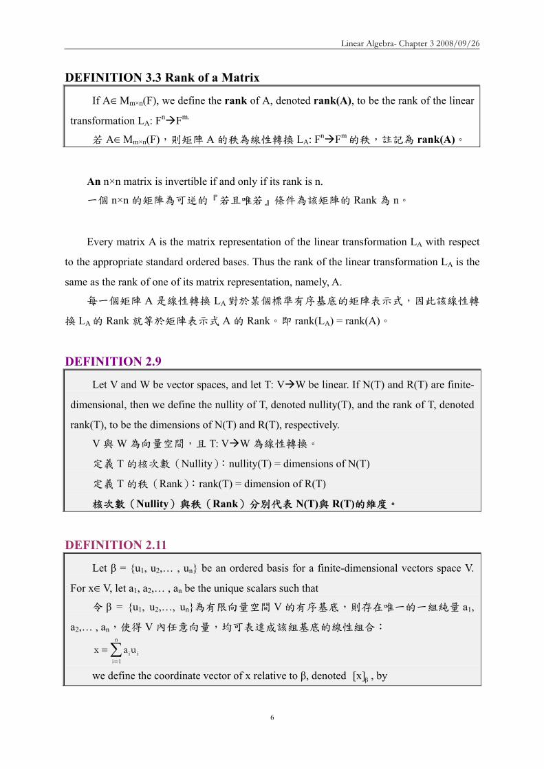
Linear Algebra- Chapter 3 20080926
6
DEFINITION 33 Rank of a Matrix
If AisinMmtimesn(F) we define the rank of A denoted rank(A) to be the rank of the linear
transformation LA Fn Fm
若 AisinMmtimesn(F)則矩陣 A 的秩為線性轉換 LA Fn Fm的秩註記為 rank(A)
An ntimesn matrix is invertible if and only if its rank is n
一個 ntimesn 的矩陣為可逆的『若且唯若』條件為該矩陣的 Rank 為 n
Every matrix A is the matrix representation of the linear transformation LA with respect
to the appropriate standard ordered bases Thus the rank of the linear transformation LA is the
same as the rank of one of its matrix representation namely A
每一個矩陣 A 是線性轉換 LA 對於某個標準有序基底的矩陣表示式因此該線性轉
換 LA的 Rank 就等於矩陣表示式 A 的 Rank即 rank(LA) = rank(A)
DEFINITION 29
Let V and W be vector spaces and let T V W be linear If N(T) and R(T) are finite-
dimensional then we define the nullity of T denoted nullity(T) and the rank of T denoted
rank(T) to be the dimensions of N(T) and R(T) respectively
V 與 W 為向量空間且 T V W 為線性轉換
定義 T 的核次數(Nullity)nullity(T) = dimensions of N(T)
定義 T 的秩(Rank)rank(T) = dimension of R(T)
核次數(Nullity)與秩(Rank)分別代表 N(T)與 R(T)的維度
DEFINITION 211
Let β = u1 u2hellip un be an ordered basis for a finite-dimensional vectors space V
For xisinV let a1 a2hellip an be the unique scalars such that
令 β = u1 u2hellip un為有限向量空間 V 的有序基底則存在唯一的一組純量 a1
a2hellip an使得 V 內任意向量均可表達成該組基底的線性組合
sum=
=n
1iiiuax
we define the coordinate vector of x relative to β denoted β[x] by
Linear Algebra- Chapter 3 20080926
7
⎟⎟⎟⎟⎟
⎠
⎞
⎜⎜⎜⎜⎜
⎝
⎛
=β
n
2
1
a
aa
[x] 稱為 x 相對於有序基底 β的座標向量
DEFINITION 212
Suppose that V and W are finite-dimensional vector spaces with ordered bases β = v1
v2hellip vn and γ = w1 w2hellip wn respectively Let T V W be linear Then for each j 1
≦j≦n there exist unique scalars aijisinF 1≦i≦m such that
sum==
m
1iiijj wa)vT( for 1≦j≦n
We call the mtimesn matrix A defined by Aij = aij the matrix representation of T in the ordered bases β and γ and write γ
β= [T]A
If V = W and β = γ then we write β= [T]A
設 V 與 W 分別為有限維度的向量空間β = v1 v2hellip vn與 γ = w1 w2hellip
wn分別為 V 與 W 的有序基底且 T V W 為 V 映至 W 的線性轉換
對每一個 j(1≦ j≦n)而言存在唯一的純量 aij isinF(1≦ i≦m)使得
sum==
m
1iiijj wa)vT(
將 mtimesn 的矩陣 A 定義為 Aij = aij並稱呼 A 為線性轉換 T 的矩陣表達方式在
V 與 W 分別以 β 與 γ作為有序基底下A 可註記為 γβ= [T]A
若 V = W 且 β = γ則 β= [T]A
提示 sum==
m
1iiijj wa)vT( 為「將 vj的像 T(vj)表達成有序基底 γ的線性組合」
DEFINITION 217
Let A be an mtimesn matrix with entries from a field F We denote by LA the mapping LA
Fn Fm defined by LA(x) = Ax (the matrix product A and x) for each column vector xisinFn
We call LA a left-multiplication transformation
令 A 是 mtimesn 的矩陣所有元素均來自 FLA為 Fn映至 Fm的線性轉換並定義為
LA(x) = Ax其中 x 為行向量(Column vector)且 xisinFnLA被稱為左乘法轉換
Linear Algebra- Chapter 3 20080926
8
The next theorem extends this fact to any matrix representation of any linear
transformation defined on finite-dimensional vector spaces
Theorem 33 Let T V W be a linear transformation between finite dimensional vector spaces and
let β and γ be ordered bases for V and W respective Then rank(T) = rank( γβ[T] )
令 T V W且 β 與 γ 分別為有限維度向量空間 V 與 W 的有序基底則
rank(T) = rank( γβ[T] )
改寫 Definition 212
Suppose that Fn and Fm are finite-dimensional vector spaces with ordered bases β =
v1 v2hellip vn and γ = w1 w2hellip wn respectively Let LA Fn Fm be linear and defined
by LA(x) = Ax Then for each j 1≦j≦n there exist unique scalars aijisinF 1≦i≦m such
that sum=
=m
1iiijjA wa)v(L for 1≦j≦n We call the mtimesn matrix A defined by Aij = aij the matrix
representation of LA in the ordered bases β and γ and write γβ= ][LA A
Now that the problem of finding the rank of a linear transformation has been reduced to
the problem of finding the rank of a matrix we need a result that allows us to perform rank-
preserving operations on matrices The next theorem and its corollary tell us how to do this
線性轉換的 Rank 可以被簡化為找矩陣的 Rank如何找矩陣的 Rank
Theorem 34 Let A be an mtimesn matrix If P and Q are invertible mtimesm and ntimesn matrices respectively
then
令 A 為 mtimesn 的矩陣若 P 與 Q 分別為可逆的 mtimesm 與 ntimesn 矩陣則
(a) rank(AQ) = rank(A)
(b) rank(PA) = rank(A)
(c) rank(PAQ) = rank(A)
【Proof】
R(LAQ) = R(LALQ) = LALQ(Fn) = LA(LQ(Fn)) = LA(Fn) = R(LA)
Since LQ is onto rank(AQ) = dim(R(LAQ)) = dim(R(LA)) = rank(A)
Linear Algebra- Chapter 3 20080926
9
rank(PAQ) = rank(PA) = rank(A)
註Theorem 34 是為後續 Reduced Row Echelon Form of Matrix 做準備一個矩陣經過
基本行運算或基本列運算或基本行與列運算後並不會改變 RANK
Corollary
Elementary row and column operations on a matrix are rank-preserving
矩陣的基本列與行運算不會改變矩陣的 Rank
此推論結果是計算反矩陣解線性方程組的重要依據
Theorem 35 The rank of any matrix equals the maximum number of its linearly independent
columns that is the rank of a matrix is the dimension of the subspace generated by its
column
任一矩陣的 Rank 等於其最大線性獨立行向量數目即矩陣的 Rank 是由矩陣的
行向量生成的子空間的維度【LA Fn Fm】
【Proof】
For any AisinMmtimesn(F)
rank(A) = rank(LA) = dim(R(LA))
Let β be the standard basis of Fn Then β spans Fn and hence by Theorem 22
R(LA ) = span(LA (β)) = span(LA(e1) LA(e2)hellip LA(en))
But for any j we have seen in Theorem 213(b) that LA(ej) = Aej = aj where aj is the
jth column of A Hence R(LA ) = span(a1 a2 an)
Thus rank(A) = rank(LA) = dim(span(a1 a2 an))
對任意矩陣 Arank(A) = rank(LA) = dim(R(LA))
令 β為 Fn 的標準基底且生成 Fn
依據 Theorem 22
LA的值域 Range 可由 LA(β)來生成
R(LA) = span(LA (β)) = span(LA(e1) LA(e2)hellip LA(en))
對任意 j 而言由 Theorem 213(b) 可知 LA(ej) = Aej = aj其中aj 為 A 的第 j
個行(aj 相當於 Theorem 213(b)的 vj 或 Theorem 22 的 T(vj))因此 R(LA) =
Linear Algebra- Chapter 3 20080926
10
span(a1 a2 an)
所以 rank(A) = rank(LA) = dimension of R(LA) = dim(span(a1a2an))
Theorem 22 令 V 與 W 為向量空間且 T V W 為線性轉換若 β = v1 v2hellip vn
是定義域(Domain)V 的基底則 T 的值域 Range R(T)可由 T(β)來生成意即 R(T)
= span(T(β)) = span(T(v1) T(v2)hellip T(vn))
Theorem 213 A 為 mtimesn 的矩陣與 B 為 ntimesp 的矩陣uj 與 vj分別為 AB 與 B 的第 j 行
(1 j p≦ ≦ )則
(a) uj = A vj
(b) vj = B ej where ej is the jth standard vector of Fp
EXAMPLE 1
Let ⎟⎟⎟
⎠
⎞
⎜⎜⎜
⎝
⎛=
101110101
A
Observe that the first and second columns of A are linearly independent and that the
third column is a linear combination of the first two Thus
A 的第一行與第二行是線性獨立第三行則是前兩行的線性組合於是
rank(A) = dim⎟⎟⎟⎟
⎠
⎞
⎜⎜⎜⎜
⎝
⎛
⎟⎟⎟
⎠
⎞
⎜⎜⎜
⎝
⎛
⎪⎭
⎪⎬
⎫
⎟⎟⎟
⎠
⎞
⎜⎜⎜
⎝
⎛
⎪⎩
⎪⎨
⎧
⎟⎟⎟
⎠
⎞
⎜⎜⎜
⎝
⎛
⎟⎟⎟
⎠
⎞
⎜⎜⎜
⎝
⎛
111
010
101
span = 2
A 的第 1 行a1=⎟⎟⎟
⎠
⎞
⎜⎜⎜
⎝
⎛
101第 2 行a2=
⎟⎟⎟
⎠
⎞
⎜⎜⎜
⎝
⎛
010第 3 行a3=
⎟⎟⎟
⎠
⎞
⎜⎜⎜
⎝
⎛
111
In order to compute the rank of a matrix A it is frequently useful to postpone the use of
Theorem 35 until A has been suitable modified by means of appropriate elementary row and
column operations so that the number of linearly independent columns is obvious
為了利用 Theorem 35 求矩陣 A 的 Rank(等於最大線性獨立行向量數目)A 可
先經過基本列或行運算使其線性獨立的行數變得比較明顯
EXAMPLE 2 Let
Linear Algebra- Chapter 3 20080926
11
⎟⎟⎟
⎠
⎞
⎜⎜⎜
⎝
⎛=
211301121
A
If we subtract the first row of A from rows 2 and 3 (type 3 elementary row operations)
the result is
⎟⎟⎟
⎠
⎞
⎜⎜⎜
⎝
⎛
minusminus
110220121
If we now substract twice the first column from the second and substract the first
column from the third (type 3 elementary column operations) we obtain
⎟⎟⎟
⎠
⎞
⎜⎜⎜
⎝
⎛
minusminus
110220001
(後二行線性相依最大線性獨立行數為 2)
It is now obvious that the maximum number of linearly independent column of this matrix is 2 Hence the rank of A is 2
Theorem 36 Let A be an mtimesn matrix of rank r Then r m r n and by means of a finite number ≦ ≦
of elementary row and column operations A can be transformed into the matrix
D = ⎟⎟⎠
⎞⎜⎜⎝
⎛
32
1r
OOOI
where O1 O2 and O3 are zero matrices Thus Dii = 1 for i r and ≦
Dij = 0 otherwise
令 A 為 Rank 等於 r 的 mtimesn 矩陣則 r m≦ 且 r n≦ 經過有限次數的基本行與列
運算讓 A 化成 D = ⎟⎟⎠
⎞⎜⎜⎝
⎛
32
1r
OOOI
其中Ir 為對角元素為 1 的對角矩陣即 A 可經
過有限次數的基本行及列運算取得沿對角線前 r 個位置皆為 1其餘各處皆為 0 的
矩陣 D
【Proof】
If A is the zero matrix r = 0 In this case the conclusion follows with D = A
若 A 為零矩陣則 r = 0 且 D = A
Now suppose that AneO and r = rank(A) then r gt 0
The proof is by mathematical induction on m the number of rows of A
若 A 非零矩陣且 r = rank(A)則 r gt 0
Linear Algebra- Chapter 3 20080926
12
採用數學歸納法
Suppose that m = 1
A can be transformed into the matrix (1 0 hellip0)
So rank(D) = rank(A) = 1 by Corollary to Theorem 34 and Theorem 35 Thus the
theorem is established for m = 1
設 m = 1則 A 可以化成(1 0 hellip0)
依據 Corollary to Theorem 34 及 Theorem 35
rank(D) = rank(A) = 1
故本定理對 m = 1 的矩陣是成立的
Next assume that the theorem holds for any matrix with at most m - 1 row (for some m
gt1)
We must prove that the theorem holds for any matrix with m rows
其次假設本定理對至多含 m - 1 列的矩陣皆成立(m gt 1)
至於含 m 列的矩陣是否成立
If n = 1 Theorem 36 can be established in a manner analogous to that for m = 1
若 n = 1則可按 m = 1 的方式證明本定理對於 n = 1 的矩陣成立
We now suppose that n gt 1 Since A ne O Aijne0 for some i j By means of at most one
elementary row and at most one elementary column operation (each of type 1) We can
move the nonzero entry to the 11 position By means of of at most one additional type 2
operation we can assure a 1 in the 11 position By means of at most m ndash 1 type 3 row
operations and at most n ndash 1 type 3 column operations we can eliminate all nonzero entries
in the first row and the first column with the exception of the 1 in the 11 postion
Thus with a finite number of elementary operation A can be transformed into a
matrix
經過有限次數的基本行及列運算可將 A 轉換成
⎪⎪⎭
⎪⎪⎬
⎫
⎪⎪⎩
⎪⎪⎨
⎧
=
0B
0001
B where Brsquo is an (m-1)times(n-1) matrix
Brsquo has rank one less than B
Brsquo的 Rank 比 B 少 1
Since rank(A) = rank(B) = r rank(Brsquo) = r ndash 1 Therefore r ndash1 ≦ m ndash 1 and r ndash1 ≦
Linear Algebra- Chapter 3 20080926
13
n ndash 1 by the induction hypothesis Hence r ≦ m and r ≦ n
由於 rank(A) = rank(B) = r故 rank(Brsquo) = r ndash 1
依數學歸納法 r ndash1 ≦ m ndash 1 且 r ndash1 ≦ n ndash 1
因此 r ≦ m 且 r ≦ n
Also by the induction hypothesis Brsquo can be transformed by a finite number of
elementary row and column operations into the (m-1)times(n-1) matrix Drsquo such that
同樣地依據數學歸納法Brsquo 可經過有限次數的基本行與列運算轉換成 (m-
1)times(n-1) 的矩陣 Drsquo使得
Dlsquo= ⎟⎟⎠
⎞⎜⎜⎝
⎛ minus
65
41r
OOOI
where O4 O5 and O6 are zero matrices
That is Drsquo consists of all zeros except for its first r-1 diagonal entries which are ones
Let
⎪⎪⎭
⎪⎪⎬
⎫
⎪⎪⎩
⎪⎪⎨
⎧
=
0D
0001
D
We see that the theorem now follows once we show that D can be obtained from B by
means of a finite number of elementary row and column operations
D 可由 B 經過有限次基本行及列運算而取得
Thus since A can be transformed into B and B can be transformed into D each by a
finite number of elementary operations A can be transformed into D by a finite number of
elementary operations
經過有限次基本行及列運算A B D
Finally since Drsquo contains ones as its first r ndash 1 diagonal entries D contains ones as its
first r diagonal entries and zeros elsewhere
最後Drsquo沿對角線前 r-1 個位置皆為 1故 D 沿對角線前 r 個位置皆為 1其餘
各處皆為 0
EXAMPLE 3 Consider the maxtrix
⎟⎟⎟⎟⎟
⎠
⎞
⎜⎜⎜⎜⎜
⎝
⎛
=
192362100280844422420
A
Linear Algebra- Chapter 3 20080926
14
By means of a succession of elementary row and column operations we can transform
A into a matrix D as in Theorem 36
透過一系列的基本行與列運算將 A 轉換成 D
D
00000001000001000001
192362100280844422420
A =
⎟⎟⎟⎟⎟
⎠
⎞
⎜⎜⎜⎜⎜
⎝
⎛
==
⎟⎟⎟⎟⎟
⎠
⎞
⎜⎜⎜⎜⎜
⎝
⎛
=
By the corollary to Theorem 34 rank(A) = rank(D) Clearly however rank(D) = 3 so rank(A) = 3
Corollary 1 Let A be an mtimesn matrix of rank r Then there exist invertible matrices B and C of sizes
mtimesm and ntimesn respectively such that D = BAC where D = ⎟⎟⎠
⎞⎜⎜⎝
⎛
32
1r
OOOI
is the mtimesn matrix
in which O1 O2 and O3 are zero matrices
令 A 為 mtimesn 的矩陣Rank 為 r存在可逆的 mtimesm 矩陣 B 與 ntimesn 矩陣 C使得
D = BAC其中D = ⎟⎟⎠
⎞⎜⎜⎝
⎛
32
1r
OOOI
為 mtimesn 的矩陣O1O2 及 O3 為零矩陣
【Proof】
By Theorem 36 A can be transformed by means of a finite number of elementary
row and column operations into the matrix D
We can appeal to Theorem 31 each time we perform an elementary operation Thus
there exist elementary mtimesm matrices E1 E2hellipEp and elementary ntimesn matrices G1
G2hellipGq such that D = EpEp-1hellipE2E1AG1G2hellipGq
By Theorem 32 each Ej and Gj is invertible Let B = EpEp-1hellipE2E1 and C =
G1G2hellipGq Then B and C are invertible and D = BAC
依據 Theorem 36A 可經過有限次的基本列與行運算化成 D
引用 Theorem 31每一次皆實施某一個基本列運算於是存在基本的 mtimesm 矩
陣 E1 E2hellip Ep 與 基 本 的 ntimesn 矩 陣 G1 G2hellip Gq 使 得 D = EpEp-
1hellipE2E1AG1G2hellipGq
依據 Theorem 32 每一個基本矩陣 Ej與 Gj 皆為可逆令 B = EpEp-1hellipE2E1 與 C =
G1G2hellipGq於是 B 與 C 皆為可逆且 D = EpEp-1hellipE2E1AG1G2hellipGq = BAC
Linear Algebra- Chapter 3 20080926
15
Theorem 31 令 AisinMmtimesn(F)並假設 B 是由 A 經實施某一基本列【或行】運算後所得
到的矩陣則存在一個 mtimesm 【或 ntimesn】基本矩陣 E使得 B = EA【或 B = AE】E
矩陣是由 Im 【或 In】 經實施與「由 A 得到 B」相同的基本列【或行】運算後所得
到的矩陣反之若 E 是一個 mtimesm【或 ntimesn】的基本矩陣則 EA【或 AE】是由 A
經過與「由 Im 【或 In】 得到 E」相同的基本列【或行】運算後所得到的矩陣
Theorem 32 基本矩陣為可逆矩陣且基本矩陣的反矩陣亦是同一型的基本矩陣
Theorem 36 令 A 為 Rank 等於 r 的 mtimesn 矩陣則 r m≦ 且 r n≦ 經過有限次數的基
本行與列運算讓 A 化成 D = ⎟⎟⎠
⎞⎜⎜⎝
⎛
32
1r
OOOI
其中Ir為對角元素為 1 的對角矩陣
Corollary 2 Let A be an mtimesn matrix Then
(a) rank(At) = rank(A)
矩陣轉置後的 RANK 不變
(b) The rank of any matrix equals the maximum number of its linearly independent
rows that is the rank of a matrix is the dimension of the subspace generated by
rows
任一矩陣的 Rank 等於最大線性獨立列向量的數目即矩陣的 Rank 等於由該
矩陣列向量所生成的子空間的維度
(c) The rows and columns of any matrix generate subspaces of the same dimension
numerically equal to the rank of the matrix
任一矩陣的列向量與行向量生成的子空間的維度相同維度等於該矩陣的
Rank
【Proof】
By Corollary 1 there exist invertible matrices B and C such that D = BAC where D
satisfies the stated conditions of the corollary Taking transposes we have
Dt = (BAC) t = CtAtBt
Since B and C are invertible so are Bt and Ct
Hence by Theorem 34 rank(At) = rank(CtAtBt) = rank(Dt)
Suppose that r = rank(A)
Then Dt is an ntimesm matrix with the form of the matrix D in Corollary 1 and hence
Linear Algebra- Chapter 3 20080926
16
rank(Dt) = r by Theorem 35
Thus
rank(At) = rank(Dt) = r = rank(A)
依據 Corollary 1存在可逆矩陣 B 與 C使得 D = BAC
取其轉置可得Dt = (BAC) t = CtAtBt
由於 B 與 C 為可逆故 Bt 與 Ct 亦為可逆
依據 Theorem 34得知 rank(At) = rank(CtAtBt) = rank(Dt)
設 r = rank(A)
則 Dt為一 ntimesm 的矩陣型式與 D 相同(參考 Corollary 1)
且依據 Theorem 35 得知 rank(Dt) = r
於是 rank(At) = rank(Dt) = r = rank(A)
Theorem 34 Let A be an mtimesn matrix If P and Q are invertible mtimesm and ntimesn matrices
respectively then 令 A 為 mtimesn 的矩陣若 P 與 Q 分別為可逆的 mtimesm 與 ntimesn 矩陣
則
(a) rank(AQ) = rank(A)
(b) rank(PA) = rank(A)
(c) rank(PAQ) = rank(A)
Theorem 35 The rank of any matrix equals the maximum number of its linearly
independent columns that is the rank of a matrix is the dimension of the subspace
generated by its column 任一矩陣的 Rank 等於其最大線性獨立行向量數目即矩陣
的 Rank 是由矩陣的行向量生成的子空間的維度【LA Fn Fm】
Corollary 3 Every invertible matrix is a product of elementary matrices
每一可逆矩陣均可為基本矩陣的乘積
【Proof】
If A is an invertible ntimesn matrix then rank(A) = n Hence the matrix D in Corollary 1
equals In and there exist invertible matrices B and C such that In = BAC
As in the proof of Corollary 1 note that B = EpEp-1hellipE2E1 and C = G1G2hellipGq where
the Eirsquos and Girsquos are elementary matrices Thus A = B-1InC-1 = B-1C-1 so that
A = E1-1E2
-1hellipEp-1Gq
-1Gq-1-1hellipG1
-1
Linear Algebra- Chapter 3 20080926
17
The inverses of elementary matrices are elementary matrices however and hence A is
the product of elementary matrices
若 A 為可逆的 ntimesn 矩陣則 rank(A) = n
因此 Corollary 1 中的矩陣 D 為 In且存在可逆的 B 與 C 矩陣使得 In = BAC
如同 Corollary 1 的證明一樣B = EpEp-1hellipE2E1 且 C = G1G2hellipGq其中Eirsquos 與
Girsquos 皆為基本矩陣
於是A = B-1InC-1 = B-1C-1即 A = E1-1E2
-1hellipEp-1Gq
-1Gq-1-1hellipG1
-1
基本矩陣的反矩陣亦為基本矩陣A 是基本矩陣的乘積
Theorem 37 Let T V W and U W Z be linear transformations on finite-dimensional vector
spaces V W and Z and let A and B be matrices such that the product AB is defined Then
令 VW 與 Z 為有限維度的向量空間T V W 與 U W Z 為線性轉換且
A 與 B 為滿足乘積 AB 定義的矩陣則
(a) rank(UT) ≦ rank(U)
(b) rank(UT) ≦ rank(T)
(c) rank(AB) ≦ rank(A)
(d) rank(AB) ≦ rank(B)
【Proof】
(a) Clearly R(T)subeW
Hence R(UT) = UT(V) = U(R(T)) sube U(W) = R(U)
Thus rank(UT) = dim(R(UT)) ≦ dim (R(U)) = rank(U)
(c) By (a) rank(AB) = rank(LAB) = rank (LALB) ≦ rank(LA) = rank(A)
(d) By (c) and Corollary 2 to Theorem 36
rank(AB) = rank((AB)t) = rank(B t A t) ≦ rank(B t) = rank (B) (b) Let α β and γ be ordered bases for V W and Z respectively and let Arsquo = γ
β]U[
and Brsquo = βα]T[ Then ArsquoBrsquo = γ
α]UT[ by Theorem 211
Hence by Theorem 33 and (d)
rank(UT) = rank(ArsquoBrsquo) ≦ rank(Brsquo) = rank (T)
Theorem 211 Let V W and Z be finite-dimensional vector space with ordered bases α β
and γ respectively Let T V W and U W Z be linear transformation Then
Linear Algebra- Chapter 3 20080926
18
βα
γβ
γα = [T][U][UT] 令 VW 與 Z 是有限維度的向量空間αβ 與 γ 分別為 VW 與
Z 的有序基底令 T V W (先 α β) 且 U W Z (後 β γ)則 βα
γβ
γα = [T][U][UT]
Theorem 33 Let T V W be a linear transformation between finite dimensional vector
spaces and let β and γ be ordered bases for V and W respective Then rank(T) = rank( γ
β[T] ) 令 T V W且 β 與 γ 分別為有限維度向量空間 V 與 W 的有序基底
則 rank(T) = rank( γβ[T] )
EXAMPLE 4
(a) Let ⎟⎟⎠
⎞⎜⎜⎝
⎛minus
=11111121
A (第一列與第二列是 LI) rank(A) = 2
(b) Let ⎟⎟⎟
⎠
⎞
⎜⎜⎜
⎝
⎛=
003011011131
A (第三列與第一二列是 LD)rank(A) = 2
(c) Let ⎟⎟⎟
⎠
⎞
⎜⎜⎜
⎝
⎛
minus=
011111121321
A (三列為 LI) rank(A) = 3
The inverse of a Matrix
We have remarked that an ntimesn matrix is invertible if and only if its rank is n Since we
know how to compute the rank of any matrix we can always test a matrix to determine
whether it is invertible We now provide a simple technique for computing the inverse of a
matrix that utilizes elementary row operations
已知 ntimesn 矩陣為可逆的『若且唯若』條件為該矩陣的 Rank 等於 n
DEFINITION 34 Augmented Matrix Let A and B be mtimesn and mtimesp matrices respectively By the augmented matrix )BA(
we mean that the mtimes(n+p) matrix )BA( that is the matrix whose first n columns are the
columns of A and whose last p columns are the columns of B 設 A 與 B 分別為 mtimesn 與 mtimesp 的矩陣則增廣矩陣(Augmented matrix) )BA(
Linear Algebra- Chapter 3 20080926
19
為一 mtimes(n+p)的矩陣 )BA( 該矩陣的前 n 行(Column)為 A 的所有的行後 p
行為 B 的所有行
Let A be an invertible ntimesn matrix and consider the ntimes2n augmented matrix C= )IA( n
C= )IA( n )AI()IAAA(CA 1
nn111 minusminusminusminus ==
By Corollary 3 to Theorem 36 A-1 is the product of elementary matrices say
A = EpEp-1hellipE2E1 (A-1 是多個基本矩陣的乘積)
Thus )AI()IAAA(CA 1
nn111 minusminusminusminus == )AI(CA)IA(EEE 1
n1
n11ppminusminus
minus ==
We have the following result If A is an invertible invertible ntimesn matrix then it is
possible to transform the matrix (AIn) into the matrix (InA-1) by means of a finite
number of elementary row operations
若 A 為一可逆的 ntimesn 矩陣則可經過有限次數的基本列運算將矩陣 (AIn) 化成
(InA-1)
Conversely suppose that A is invertible and that for some ntimesn matrix B the matrix
(AIn) can be transformed into the matrix (InB) by a finite number of elementary row
operations Let E1 E2hellip Ep be the elementary matrices associated with these elementary row
operations as in Theorem 31 then
反之假設 A 是可逆且矩陣(AIn)可經有限次數的基本列運算轉換成矩陣(InB)
並令 E1 E2hellip Ep 分別為 Theorem 31 所稱的基本矩陣則
)BI()IA(EEE nn11pp =minus
Let M = EpEp-1hellipE2E1 we have 令 M = EpEp-1hellipE2E1
)BI()IA(EEE nn11pp =minus )BI()IA(M)MMA( nn ==
Linear Algebra- Chapter 3 20080926
20
Hence MA = In and M = B It follows that M = A-1 So B = A-1
可由 MA = In 及 M = B 得知M 就是 A-1故 B 就是 A-1
Thus we have the follow resultsIf A is an invertible ntimesn matrix and the matrix
(AIn) is transformed in a matrix of the form (InB) by means of a finite number of
elementary row operations then B=A-1
若 A 為一可逆的 ntimesn 矩陣且矩陣 (AIn) 可經有限次數的基本列運算化成
(InB)則 B=A-1
If on the other hand A is an ntimesn matrix that is not invertible then rank(A) lt n Hence
any attempt to transform (AIn) into a matrix of the form (InB) by means of elementary row
operations must fail
反之若 A 是一不可逆的 ntimesn 矩陣則 rank(A) lt n因此任何想利用基本列運算
要將矩陣 (AIn) 化成 (InB)的努力必定失敗
Thus we have the follow results If A is an notinvertible ntimesn matrix then any attempt
to transform (AIn) into a matrix of the form (InB) produce a row whose first n entries
are zeros
若 A 是一不可逆的 ntimesn 矩陣任何想將矩陣 (AIn) 化成 (InB)的努力最後會
產生一前 n 個元素均為 0 的列
EXAMPLE 5
We determine whether the matrix ⎟⎟⎟
⎠
⎞
⎜⎜⎜
⎝
⎛=
133242420
A is invertible and if it is we
compute its inverse
A 是否為可逆矩陣
We attempt to use elementary row operations to transfer
Linear Algebra- Chapter 3 20080926
21
⎟⎟⎟
⎠
⎞
⎜⎜⎜
⎝
⎛=
100010001
133242420
)IA( into a matrix of the form (InB)
看看能否利用基本行與列運算將矩陣 (AIn) 化成 (InB)
Interchanging rows 1 and 2
⎟⎟⎟
⎠
⎞
⎜⎜⎜
⎝
⎛
100001010
133420242
Multiplying the first row by 12
⎟⎟⎟
⎠
⎞
⎜⎜⎜
⎝
⎛
10000100
133420121 2
1
Adding -3 times row 1 to row 3
⎟⎟⎟
⎠
⎞
⎜⎜⎜
⎝
⎛
minusminusminus 1000100
230420121
23
21
Multiplying row 2 by 12 to obtain 1 in the 22 position
⎟⎟⎟
⎠
⎞
⎜⎜⎜
⎝
⎛
minus
minus
minusminus 100000
230210121
23
21
21
Adding -2 times row 2 to row 1 and 3 times row 2 to row 3
⎟⎟⎟
⎠
⎞
⎜⎜⎜
⎝
⎛
minus
minusminus
10001
400210301
23
2321
21
Multiplying row 3 by 14
⎟⎟⎟
⎠
⎞
⎜⎜⎜
⎝
⎛
minus
minusminus
41
83
8321
21
0001
100210301
Adding appropriate multiply of row 3 to row 1 and 2 completes the process
⎟⎟⎟
⎠
⎞
⎜⎜⎜
⎝
⎛
minusminus
minus
41
83
83
21
43
41
43
85
81
100010001
目標達成
Thus A is invertible and ⎟⎟⎟
⎠
⎞
⎜⎜⎜
⎝
⎛
+minus+minus+minus+minus+
=minus
41
83
83
21
43
41
43
85
81
1A
Linear Algebra- Chapter 3 20080926
22
EXAMPLE 6
We determine whether the matrix ⎟⎟⎟
⎠
⎞
⎜⎜⎜
⎝
⎛minus=451112
121A is invertible and if it is we
compute its inverse
A 是否為可逆矩陣
We attempt to use elementary row operations to transfer
⎟⎟⎟
⎠
⎞
⎜⎜⎜
⎝
⎛minus=
100010001
451112
121)IA( into a matrix of the form (InB)
看看能否利用基本行與列運算將矩陣 (AIn) 化成 (InB)
Adding -2 times row 1 to row 2 and -1 times row 1 to row 3 then addig row 2 to row
3
⎟⎟⎟
⎠
⎞
⎜⎜⎜
⎝
⎛minus
100010001
451112
121
⎟⎟⎟
⎠
⎞
⎜⎜⎜
⎝
⎛
minusminusminusminus
101012001
330330
121
⎟⎟⎟
⎠
⎞
⎜⎜⎜
⎝
⎛
minusminusminusminus
113012001
000330
121
is a matrix with row whose first 3 entries are zeros Therefore A is not invertible
最後一列前 3 個元素均為 0
EXAMPLE 7 Let T P2(R) P2(R) be defined by T(f(x)) = f(x)+frsquo(x)+frdquo(x) where frsquo(x) and frdquo(x)
denote the first and second derivatives of f(x) We use Corollary 1 to Theorem 218 to test
T for invertibility and compute the inverse if T is invertible Taking β=1 x x2 to be the
standard ordered basis of P2(R) we have
令 T P2(R) P2(R) 為線性轉換且定義為 T(f(x)) = f(x)+frsquo(x)+frdquo(x)利用
Corollary 1 to Theorem 218 來測試 T 是否可逆並計算其逆轉換取 β=1 x x2為
P2(R)的標準有序基底
T(1) = 1 = 1bull1+0bullx+0bullx2
T(x) = 1+x = 1bull1+1bullx+0bullx2
Linear Algebra- Chapter 3 20080926
23
T(x2) = 2+2x+x2 = 2bull1+2bullx+1bullx2
⎟⎟⎟
⎠
⎞
⎜⎜⎜
⎝
⎛=β
100210211
[T] 稱為 T 相對有序基底 β的座標向量
依據 Corollary 1 to Theorem 218 T 可逆『若且唯若』 β[T] 可逆且
1-1 )[T](][T minusββ =
Using the method of Examples 5 and 6 we can show that β[T] is invertible with
inverse
⎟⎟⎟
⎠
⎞
⎜⎜⎜
⎝
⎛minus
minus=minus
β
100210
011)([T] 1
Thus T is is invertible and βminusminus
β = ][T)([T] 11 Hence by Theorem 214 we have
⎟⎟⎟
⎠
⎞
⎜⎜⎜
⎝
⎛minusminus
=⎟⎟⎟
⎠
⎞
⎜⎜⎜
⎝
⎛
⎟⎟⎟
⎠
⎞
⎜⎜⎜
⎝
⎛minus
minus=++ β
minus
2
21
10
2
1
02
2101
aa2aaa
aaa
100210
011)]xaxa(a[T
Therefore T-1(a0+a1x+a2x2) = (a0-a1)+(a1-2a2)x+a2x2 Corollary 1 to Theorem 218 Let V be finite-dimensional vector space with an ordered basis β and let T V V be linear Then T is invertible if and only if β[T] is invertible
Furthermore 1-1 )[T](][T minusββ = V 為有限維度的向量空間β 是 V 的有序基底令 T
V V 為線性轉換 T 為可逆的『若且唯若』條件為 β[T] 可逆再者
1-1 )[T](][T minusββ =
Theorem 214 Let V and W be finite-dimensional vector spaces having ordered bases β and γ respectively and let T V W be linear Then for each uisinV we have β
γβγ = [u][T][T(u)]
V 與 W 為有限維度的向量空間β 與 γ分別 V 與 W 的有序基底令 T V W 為線
性轉換則 V 中的 u 映至 W 的結果 T(u) 相對於有序基底 γ 的座標向量為
βγβγ = [u][T][T(u)]
Invertible and Inverse of MATRIX Let A be an n times n matrix If a matrix B can be found such that AB = BA = In then A is
Linear Algebra- Chapter 3 20080926
24
said to be invertible and B is called the inverse of A (denote B = A-1 and A-k=(A-1)k )
If such a matrix B does not exist then A has no inverse
EXAMPLE
⎥⎦
⎤⎢⎣
⎡=
4321
A and ⎥⎦
⎤⎢⎣
⎡minus
minus=
21
23
12B
221
23
221
23
I1001
432112
BA
I100112
4321
AB
=⎥⎦
⎤⎢⎣
⎡=⎥
⎦
⎤⎢⎣
⎡⎥⎦
⎤⎢⎣
⎡minus
minus=
=⎥⎦
⎤⎢⎣
⎡=⎥
⎦
⎤⎢⎣
⎡minus
minus⎥⎦
⎤⎢⎣
⎡=
Thus AB = BA = I2 proving that the matrix A has inverse B
Theorem The inverse of an invertible matrix is unique
Let B and C be inverse of A
Thus AB = BA = In and AC = CA = In
Multiply both sides of the equation AB = In by C
C(AB) = CIn (CA)B = C
InB = C B = C
Thus an invertible matrix has only one inverse
How to find AHow to find A--11
Based on the GaussBased on the Gauss--Jordan algorithmJordan algorithmLet A be an invertible matrix Then AALet A be an invertible matrix Then AA--11=I=Inn
Let the columns of Let the columns of AA--11 be be XX11 XX22 helliphellip XXnn and the columns of I and the columns of Inn be be CC11CC22helliphellipCCnn
Find AFind A--11 by finding by finding XX11 XX22 helliphellip XXnn Write the equation AAWrite the equation AA--11=I=Inn in the formin the form
[ ] [ ]n21nn211 CCCI XXXALet LL ==minus
[ ] [ ][ ] [ ]n21n21
n21n21
CCCAXAXXACCCXXXALL
LL
=rArr=
nn2211 CAXCAX CAX === LThus
How to find AHow to find A--11
Solving these systems by using Gauss-Jordan elimination on the large augmented matrix [AC1 C2hellipCn]
Thus when A-1 exits
[ ] [ ] [ ] 1n
1nn ABwhereBIAIIA minusminus ==asympasympL
If the reduced echelon form of [If the reduced echelon form of [AIAInn] is computed and ] is computed and the first part is not of the form Ithe first part is not of the form Inn then A has no inversethen A has no inverse
[ ][ ]n21n
n21
XXXI CCCAmatrix augmented
LL
L
asympasymp
Linear Algebra- Chapter 3 20080926
25
Example Example 1212
⎥⎥⎥
⎦
⎤
⎢⎢⎢
⎣
⎡
minusminusminusminusminus
=100531010532001211
]IA[ 3
⎥⎥⎦
⎤
⎢⎢⎣
⎡minusminusminus
minusminus
+minus+
asymp
101320012110001211
1RR1R3
2)(R2
⎥⎥⎦
⎤
⎢⎢⎣
⎡minus
minusminusminusasymp
101320012110001211
R2)1(
⎥⎥⎥
⎦
⎤
⎢⎢⎢
⎣
⎡
minusminusminusminusminus
=531532211
ADetermine the inverse of
Example Example 2222
⎥⎥⎦
⎤
⎢⎢⎣
⎡
minusminusminusminus
minus++asymp
123100012110013101
R2)2(R3R2R1
⎥⎥⎦
⎤
⎢⎢⎣
⎡
minusminusminus
minus++asymp
123100135010010001
R3)1(R2R3R1
123135110
A 1
⎥⎥⎥
⎦
⎤
⎢⎢⎢
⎣
⎡
minusminusminus=minus
⎥⎥⎦
⎤
⎢⎢⎣
⎡
minusminus
minus
+minus+asymp
135000011210012301
3R2R3R2)1(R1
ExampleExampleDetermine the inverse of
⎥⎥⎦
⎤
⎢⎢⎣
⎡
minus=
412721511
A
⎥⎥⎦
⎤
⎢⎢⎣
⎡
minus=
100412010721001511
][ 3IA
⎥⎥⎦
⎤
⎢⎢⎣
⎡
minusminusminusminus
minus+minus+asymp
102630011210001511
R1)2(R31)R1(R2
There is no need to proceed further There is no need to proceed further The reduced echelon form cannot have a one in the (3 3) locatioThe reduced echelon form cannot have a one in the (3 3) location n
The reduced echelon form cannot be of the form [IThe reduced echelon form cannot be of the form [Inn B] B] Thus Thus AAndashndash11 does not existdoes not exist
Properties of Matrix InverseProperties of Matrix Inverse
Let Let AA and and BB be invertible matrices andbe invertible matrices and cc a nonzero scalar a nonzero scalar ThenThen
AA =minusminus 11)( 111 1)( 2 minusminus = A
ccA
111)( 3 minusminusminus = ABAB
nn AA )()( 4 11 minusminus =tt AA )()( 5 11 minusminus =
Color Models Color Models 1212
A color model in the context of graphics is a method of A color model in the context of graphics is a method of implementing colorsimplementing colorsThe common used models include RGB model and YIQ modelThe common used models include RGB model and YIQ modelThe RGB model is used in computer monitors and the YIQ model The RGB model is used in computer monitors and the YIQ model is used in television screensis used in television screensAn RGB computer signal can be converted to a YIQ television An RGB computer signal can be converted to a YIQ television signal using the matrix transformationsignal using the matrix transformation
⎥⎥⎥
⎦
⎤
⎢⎢⎢
⎣
⎡
⎥⎥⎥
⎦
⎤
⎢⎢⎢
⎣
⎡
minusminusminus=
⎥⎥⎥
⎦
⎤
⎢⎢⎢
⎣
⎡
BGR
311523212321275596
114587299
QIY
YIQgtRGBYIQgtRGB
Color Models Color Models 2222
A signal is converted from a television screen to a computer monA signal is converted from a television screen to a computer monitor itor using inverse of the above matrixusing inverse of the above matrix
⎥⎥⎥
⎦
⎤
⎢⎢⎢
⎣
⎡
⎥⎥⎥
⎦
⎤
⎢⎢⎢
⎣
⎡
minusminusminus=
⎥⎥⎥
⎦
⎤
⎢⎢⎢
⎣
⎡rArr
⎥⎥⎥
⎦
⎤
⎢⎢⎢
⎣
⎡
⎥⎥⎥
⎦
⎤
⎢⎢⎢
⎣
⎡
minusminusminus=
⎥⎥⎥
⎦
⎤
⎢⎢⎢
⎣
⎡minus
QIY
0751108116472721
6209561
BGR
QIY
311523212321275596
114587299
BGR 1
CryptographyCryptography 密碼學密碼學 1212
Cryptography is the process of coding and decoding messagesCryptography is the process of coding and decoding messagesThe technique can be traced back to the ancient Greeks Today The technique can be traced back to the ancient Greeks Today governments use sophisticated methods of coding and decoding governments use sophisticated methods of coding and decoding messagesmessagesOne type of code that is extremely difficult to break makes use One type of code that is extremely difficult to break makes use of a of a large matrix to encode a message large matrix to encode a message The receiver of the message decodes it using the inverse of the The receiver of the message decodes it using the inverse of the matrixmatrixThe first matrix is called the encoding matrix and its inverse The first matrix is called the encoding matrix and its inverse is is called the decoding matrixcalled the decoding matrix
Cryptography Cryptography 密碼學密碼學 2222
A A-1Message
Encoding MatrixEncoding Matrix
Decoded MessageTransmission
Decoding MatrixDecoding Matrix
Linear Algebra- Chapter 3 20080926
26
Example Example 1212
Let the message be Let the message be BUY IBM STOCKBUY IBM STOCKAnd the encoding matrix beAnd the encoding matrix be
⎥⎥⎥
⎦
⎤
⎢⎢⎢
⎣
⎡ minusminusminus
434110433
B U Y B U Y -- I B M I B M -- S T O C KS T O C K2 21 25 27 9 2 13 27 19 20 15 3 112 21 25 27 9 2 13 27 19 20 15 3 11
⎥⎥⎥
⎦
⎤
⎢⎢⎢
⎣
⎡ minusminusminusminusminus=
⎥⎥⎥
⎦
⎤
⎢⎢⎢
⎣
⎡
⎥⎥⎥
⎦
⎤
⎢⎢⎢
⎣
⎡ minusminusminus
2331372091431715418461146
222117196116169
27319225271527921112013272
434110433
EncodingEncoding
Example Example 2222
Let the message be Let the message be BUY IBM STOCKBUY IBM STOCKAnd the decoding matrix beAnd the decoding matrix be
⎥⎥⎥
⎦
⎤
⎢⎢⎢
⎣
⎡
minusminus 334344101
B U Y B U Y -- I B M I B M -- S T O C KS T O C K2 21 25 27 9 2 13 27 19 20 15 3 112 21 25 27 9 2 13 27 19 20 15 3 11
⎥⎥⎥
⎦
⎤
⎢⎢⎢
⎣
⎡=
⎥⎥⎥
⎦
⎤
⎢⎢⎢
⎣
⎡ minusminusminusminusminus
⎥⎥⎥
⎦
⎤
⎢⎢⎢
⎣
⎡
minusminus 27319225271527921112013272
2331372091431715418461146
222117196116169
334344101
DecodingDecoding
3-3 Systems of Linear Equations ndash Theoretical Aspects
The system of equations
mnmn22m11m
2nn2222121
1nn1212111
bxaxaxa
bxaxaxabxaxaxa
=+++
=+++=+++
(S)
were aij and bi (1≦i≦m and 1≦j≦n) are scalars in a field F and x1 x2hellipxn are n
variables taking values in F is called a system of m linear equations in n unknows over the
field F
上式稱為佈於 Field F 含有 n 個未知數m 個線性方程式的系統或方程組(system
of m linear equations in n unknows)
The mtimesn matrix
⎟⎟⎟⎟⎟
⎠
⎞
⎜⎜⎜⎜⎜
⎝
⎛
=
mn2m1m
n22221
n11211
aaa
aaaaaa
A is called the coefficient matrix of the
system (S)(係數矩陣) If we let
⎟⎟⎟⎟⎟
⎠
⎞
⎜⎜⎜⎜⎜
⎝
⎛
=
n
2
1
x
xx
x and
⎟⎟⎟⎟⎟
⎠
⎞
⎜⎜⎜⎜⎜
⎝
⎛
=
m
2
1
b
bb
b Then the system (S) may
be rewritten as a single matrix equation Ax = b(單一矩陣方程式)
To exploit the results that we have developed we often consider a system of linear
equations as a single matrix equation
Linear Algebra- Chapter 3 20080926
27
A solution to the system (S) is an n-tuple n
n
2
1
F
s
ss
s isin
⎟⎟⎟⎟⎟
⎠
⎞
⎜⎜⎜⎜⎜
⎝
⎛
= such that As = b The set of
all solutions to the system (S) is called the solution set of the system(解集合) System (S)
is called consistent(相容) if its solution set is nonempty otherwise it is called
inconsistent(不相容)
方程組(S)的解為一 n 序組該序組可以使 As = b方程組的所有解所成的集合
稱為該方程組的解集合(Solution set)方程組的解集合非空集合者稱為「相容」解
集合空集合者稱為「不相容」
EXAMPLE 1
Consider 6x2xx1xx3x2
321
321
=+minus=++
that is ⎟⎟⎠
⎞⎜⎜⎝
⎛=
⎟⎟⎟
⎠
⎞
⎜⎜⎜
⎝
⎛
⎟⎟⎠
⎞⎜⎜⎝
⎛minus 6
1
xxx
211132
3
2
1
(以矩陣表示)
This system has many solutions such as ⎟⎟⎟
⎠
⎞
⎜⎜⎜
⎝
⎛minus=
726
s and ⎟⎟⎟
⎠
⎞
⎜⎜⎜
⎝
⎛
minusminus=
34
8s
Consider 1xx0xx
21
21
=+=+
that is ⎟⎟⎠
⎞⎜⎜⎝
⎛=⎟⎟
⎠
⎞⎜⎜⎝
⎛⎥⎦
⎤⎢⎣
⎡10
xx
1111
2
1
顯然地方程組無解
We begin our study of system of linear equations by examining the class of
homogeneous system of linear equations 先討論齊次方程組
DEFINITION 35 Homogeneous amp Nonhomogeneous
A system Ax=b of m linear equations in n unknowns is said to be homogeneous if b=0
Otherwise the system is said to be nonhomogeneous
方程組 Ax = bb = 0 稱為齊次方程組否則稱為非齊次方程組
Any homogeneous system has at least one solution namely the zero vector The next
result gives further information about the set of solutions to a homogeneous system
Linear Algebra- Chapter 3 20080926
28
齊次方程組至少有一個解那就是『零向量』
Theorem 38 Let Ax = 0 be a homogeneous system of m linear equations in n unknowns over a field
F Let K denote the set of all solutions to Ax = 0 Then K = N(LA) hence K is a subspace
of Fn of dimension n - rank(LA) = n- rank(A)
令 Ax = 0 代表一佈於 Field 含有 n 個未知數m 個線性方程式的方程組若令
K 代表該方程組的解集合(Solution set)則 K = N(LA)K 為 Fn 內的子空間且其維
度為 n ndash rank (LA) = n - rank(A)
【Proof】
Clearly K = sisinFn As = 0 = N(LA) The second part now follows from the
dimension theorem
Nullity(T)+rank(T) = dim(V)
Nullity (LA) = dim (Fn) ndashrank (LA ) = n ndash rank (A)
DEFINTION 27 Let V and W be vector space and let T V W be linear We define
the null space (or kernel) N(T) of T to be the set of all vectors x in V such that T(x) = 0
that is N(T) = xisinV T(x) = 0 V 與 W 為向量空間且 T V W 為線性轉換定義
線性轉換 T 的 Null space 為 V 內所有滿足 T(x) = 0 的向量 x 所形成的集合註記為
N(T)Null space 的元素 x 經線性轉換 T 轉換後所對應的「像」為 0意即 T(x) = 0
Null space 內的元素的「像」皆為 0
DEFINITION 217 Let A be an mtimesn matrix with entries from a field F We denote by LA
the mapping LA Fn Fm defined by LA(x) = Ax (the matrix product A and x) for each
column vector xisinFn We call LA a left-multiplication transformation 令 A 是 mtimesn
的矩陣所有元素均來自 FLA 為 Fn 映至 Fm的線性轉換並定義為 LA(x) = Ax其中
x 為行向量(Column vector)且 xisinFnLA被稱為左乘法轉換
Theorem 23 (Dimension Theorem) Let V and W be vector spaces and let T V W be
linear If V is finite-dimensional then Nullity(T) + rank(T) = dim(V) T 的核次數
(Nullity)與秩(Rank)的和等於定義域的維度 dim(V)
Corollary Let Ax = 0 be a homogeneous system of m linear equations in n unknowns over a field
Linear Algebra- Chapter 3 20080926
29
F If m lt n the system Ax = 0 has a nonzero solution
令 Ax = 0 代表一佈於 Field 含有 n 個未知數m 個線性方程式的方程組若 m
lt n則該方程組具有一非零解
【Proof】
Suppose that m lt n Then rank(A) = rank (LA)≦m Hence dim(K) = n - rank(LA) ≧
n ndash m gt 0 where K = N(LA) Since dim(K) gt 0 Kne 0 Thus there exists a nonzero
vector sisinK so s is a nonzero solution to Ax = 0
設 m lt n則 rank(A) = rank (LA) ≦ m依據 Theorem 38K = sisinFn As = 0
= N(LA) = dim(K) = n - rank(LA) ≧ n ndash m gt 0表示 dim(K) gt 0Kne 0故存在非
零向量 s使得 Ax = 0
EXAMPLE 2
Consider 0xxx
0xx2x
321
321
=minusminus=++
Let ⎟⎟⎠
⎞⎜⎜⎝
⎛minusminus
=111
121A be the coefficient matrix of this system It is clear that rank(A)
= 2 If K is the solution set of this system then dim(K) = 3-2 = 1 Thus any nonzero
solution constitutes a basis for K
若 K 是方程組的解所組成的集合(簡稱為解集合)依 Theorem 38 得知 dim(K)
= 3 - 2 = 1因此任一非零解將形成 K 的基底
For example since ⎟⎟⎟
⎠
⎞
⎜⎜⎜
⎝
⎛minus32
1 is a solution to the given system
⎪⎭
⎪⎬
⎫
⎪⎩
⎪⎨
⎧
⎟⎟⎟
⎠
⎞
⎜⎜⎜
⎝
⎛minus32
1 is a basis for
K Thus any vector in K is of the form ⎟⎟⎟
⎠
⎞
⎜⎜⎜
⎝
⎛minus=
⎟⎟⎟
⎠
⎞
⎜⎜⎜
⎝
⎛minus
t3t2
t
32
1t where tisinR
例如因⎟⎟⎟
⎠
⎞
⎜⎜⎜
⎝
⎛minus32
1是方程組的一個解故
⎪⎭
⎪⎬
⎫
⎪⎩
⎪⎨
⎧
⎟⎟⎟
⎠
⎞
⎜⎜⎜
⎝
⎛minus32
1 為 K 的基底K 內的任一向量均
具有如下形式
⎟⎟⎟
⎠
⎞
⎜⎜⎜
⎝
⎛minus=
⎟⎟⎟
⎠
⎞
⎜⎜⎜
⎝
⎛minus
t3t2
t
32
1t
Linear Algebra- Chapter 3 20080926
30
We now turn to the study of nonhomogeneous systems Our next result shows that the
solution set of a nonhomogeneous system Ax = b can be described in terms of the solution of
the homogeneous system Ax = 0 We refer to the equation Ax = 0 as the homogeneous system
corresponding to Ax = b
以下將進一步探討「非齊次方程組」非齊次方程組 Ax = b 的解集合可利用齊次方
程組 Ax = 0 的解來加以說明因此我們可將 Ax = 0 視為 Ax = b 的齊次方程組
Theorem 39 Let K be the solution set of a system of linear equations Ax = b and let KH be the
solution set of the corresponding homogeneous system Ax = 0 Then for any solution s to
Ax = b K =s + KH = s+k kisinKH
設 K 為線性方程組 Ax = b 的解集合且 KH為對應的齊次方程組的解集合則
對 Ax = b 的任一個解 s 而言K =s + KH = s+k kisinKH
【Proof】
Let s be any solution to Ax = b
We must show that K =s + KH
If wisinK then Aw = b Hence
A(w - s) = Aw ndash As = b ndash b = 0
So w - sisinKH
Thus there exists kisinKH such that w - s = k
It follows that w = s + k isin s +KH and therefore Ksube s +KH
Conversely suppose that wisins +KH then w = s + k for some kisinKH
But then Aw = A(s + k) = As + Ak = b + 0 = b so wisinK
Therefore s +KHsubeK and thus K=s +KH
令 s 為 Ax = b 的任一個解我們必須證明「K =s + KH」
若 wisinK則 Aw = b(即 w 為 Ax = b 的解)
於是 A(w - s) = Aw ndash As = b ndash b = 0
所以 w - sisinKH(即 w-s 為 Ax = 0 的解)
w - s 既然是 KH的元素表示有一元素 kisinKH使得 w - s = kw = s + k
w = s + kisins +KH
Linear Algebra- Chapter 3 20080926
31
因此 Ksube s +KH
反之假設 wisins +KH則 KH中存在一元素 k(kisinKH)使得 w = s + k
因 Aw = A(s + k) = As + Ak = b + 0 = b
故 wisinK 是 Ax = b 的解
因此s +KHsubeK
總結K=s +KH
EXAMPLE 3
Consider 4xxx7xx2x
321
321
minus=minusminus=++
The corresponding homogeneous system is the system in Example 2 It is easily
verified that ⎟⎟⎟
⎠
⎞
⎜⎜⎜
⎝
⎛=
411
s is a solution to the preceeding nonhomogeneous system So the
solution set of the system is ⎪⎭
⎪⎬
⎫
⎪⎩
⎪⎨
⎧isin
⎟⎟⎟
⎠
⎞
⎜⎜⎜
⎝
⎛minus+
⎟⎟⎟
⎠
⎞
⎜⎜⎜
⎝
⎛= Rt
32
1t
411
K by Theorem 39
⎟⎟⎟
⎠
⎞
⎜⎜⎜
⎝
⎛=
411
s 是非齊次方程組 Ax = b 的解
⎟⎟⎟
⎠
⎞
⎜⎜⎜
⎝
⎛minus32
1是齊次方程組的解
依據 Theorem 39 得知線性方程組 Ax = b 的解集合⎪⎭
⎪⎬
⎫
⎪⎩
⎪⎨
⎧isin
⎟⎟⎟
⎠
⎞
⎜⎜⎜
⎝
⎛minus+
⎟⎟⎟
⎠
⎞
⎜⎜⎜
⎝
⎛= Rt
32
1t
411
K
The following theorem will provide us with a means of computing solutions to certain
system of linear equations
Theorem 310~311 提供計算線性方程組的解的方法
Theorem 310 Let Ax = b be a system of n linear equations in n unknowns If A is invertible then the
Linear Algebra- Chapter 3 20080926
32
system has exactly one solution namely A-1b Conversely if the system has exactly one
solution then A is invertible
令 Ax = b 為含 n 個未知數n 個線性方程式的方程組若 A 為可逆則方程組
恰有一個解解為 A-1b反之若該方程組恰有一個解則 A 為可逆
【Proof】
Suppose that A is invertible
Substituting A-1b into system we have A(A-1b)=( AA-1)b = b
Thus A-1b is a solution
If s is an arbitrary solution then As = b
Multiplying both sides by A-1 gives s= A-1b
Thus the system has one and only one solution namely A-1b
假設 A 為可逆將 A-1b 代入方程組可得 A(A-1b)=( AA-1)b = b
故 A-1b 確為方程組的解
若 s 為方程組的任意解則 As = b
兩邊乘上 A-1可得 s= A-1b
因此方程組僅有唯一的解 A-1b
Conversely suppose that the system has exactly one solution s
Let KH denot the solution set for the corresponding homogeneous system Ax = 0
By Theorem 39 s = s + KH But it is so only if KH = 0 Thus N(LA) = 0 and
hence A is invertible
反之假設方程組恰有一個解 s
令 KH為相對應齊次方程組 Ax = 0 的解集合
依據 Theorem 39要能s = s + KH唯有 KH = 0
KH = 0即表示 N(LA) = 0故 A 為可逆
EXAMPLE 4 Consider the following system of three linear equations in three unknowns
1xx3x33x2x4x2
2x4x2
321
321
32
=++=++
=+
In Example 5 of Section 32 we compute the inverse of the coefficient matrix A of
this system Thus the system has exactly one solution namely
Linear Algebra- Chapter 3 20080926
33
⎟⎟⎟
⎠
⎞
⎜⎜⎜
⎝
⎛=
133242420
A⎟⎟⎟
⎠
⎞
⎜⎜⎜
⎝
⎛
+minus+minus+minus+minus+
=minus
41
83
83
21
43
41
43
85
81
1A
⎟⎟⎟
⎠
⎞
⎜⎜⎜
⎝
⎛
minus+minus
=⎟⎟⎟
⎠
⎞
⎜⎜⎜
⎝
⎛
⎟⎟⎟
⎠
⎞
⎜⎜⎜
⎝
⎛
+minus+minus+minus+minus+
==⎟⎟⎟
⎠
⎞
⎜⎜⎜
⎝
⎛minus
814587
41
83
83
21
43
41
43
85
81
1
3
2
1
132
bAxxx
Theorem 311 Let Ax = b be a system of linear equations Then the system is consistent (相容)if
and only if rank(A) = rank (A∣b) Matrix (A b) is called the augmented matrix o∣ f the
system Ax = b
令 Ax = b 為線性方程式方程組則此方程組至少有一個解的『若且唯若』條件
為 rank(A) = rank (A∣b) 矩陣(A∣b)稱為方程組 Ax = b 的增廣矩陣
【Proof】
To say that Ax = b has a solution is equivalent to saying that bisinR(LA)
In the proof of Theorem 35 we saw that R(LA ) = span(a1 a2 an) the span of the
column of A
Thus Ax = b has a solution if and only if bisinspan(a1 a2 an)
But bisinspan(a1 a2 an) if and only if span(a1 a2 an) = span(a1 a2 an b)
This last statement is equivalent to
dim (span(a1a2an)) = dim (span(a1a2an b))
So by Theorem 35 the preceeding equation reduces to rank(A) = rank (A∣b)
Ax = b 有一解相當於 bisinR(LA)即 b 屬於線性轉換 LA的 Range
在 Theorem 35 的證明中提到 R(LA ) = span(a1a2an)aj 為 A 的第 j 個行
(Column)即線性轉換 LA 的 Range 係由矩陣 A 的行(Column)所生成
因此 Ax = b 要有一個解的『若且唯若』條件為 bisinspan(a1 a2 an)
至於 bisinspan(a1 a2 an)之條件
bisinspan(a1a2an) 的『若且唯若』條件為 span(a1a2an) = span(a1a2an
b)
其條件相當於
Linear Algebra- Chapter 3 20080926
34
dim (span(a1a2an)) = dim (span(a1a2an b))
依據 Theorem 35該條件可簡化為 rank(A) = rank (A∣b)
Theorem 35 The rank of any matrix equals the maximum number of its linearly
independent columns that is the rank of a matrix is the dimension of the subspace
generated by its column任一矩陣的 Rank 等於其最大線性獨立行向量數目即矩陣的
Rank 是由矩陣的行向量生成的子空間的維度【LA Fn Fm】
EXAMPLE 5 Recall the system of equations
1xx0xx
21
21
=+=+
Since ⎟⎟⎠
⎞⎜⎜⎝
⎛=
1111
A and ⎟⎟⎠
⎞⎜⎜⎝
⎛=
111011
)bA(
rank(A) = 1 and rank (A b) = 2∣
Because the two ranks are unequal the system has no solutions
矩陣 A 與增廣矩陣(A∣b) 的 Rank 不同故方程組沒有解
EXAMPLE 6 We can use Theorem 311 to determine whether (3 3 2) is in the range of the linear
transformation T R3 R3 defined by T(a1 a2 a3) = (a1+a2+a3 a1-a2+a3 a1+a3)
利用 Theorem 311 來判斷 (3 3 2)是否在線性轉換 T 的 Range 中其中T R3
R3 定義為 T(a1 a2 a3) = (a1+a2+a3 a1-a2+a3 a1+a3)
Now (3 3 2)isinR(T) if and only if there exists a vector s = x1 x2 x3 in R3 such that
T(s)=(3 3 2) Such a vector s must be a solution to the system
2xx3xxx3xxx
31
321
321
=+=+minus=++
Since the ranks of the coefficient matrix and the augmented matrix of this system
are 2 and 3 respectively it follows that this system has no solutions Hence (3 3 2) notin
R(T)
(3 3 2)isinR(T) 的『若且唯若』的條件為存在一向量 s = x1 x2 x3isinR3 使得
T(s)=(3 3 2)
Linear Algebra- Chapter 3 20080926
35
向量 s 必須是 2xx3xxx3xxx
31
321
321
=+=+minus=++
的解
因係數矩陣⎟⎟⎟
⎠
⎞
⎜⎜⎜
⎝
⎛minus
101111111
的 Rank 為 2增廣矩陣⎟⎟⎟
⎠
⎞
⎜⎜⎜
⎝
⎛minus
233
101111111
的 Rank 為 3兩
者不相等故方程組無解(3 3 2) notin R(T)
Theorem 311 Let Ax = b be a system of linear equations Then the system is consistent
(相容)if and only if rank(A) = rank (A∣b) Matrix (A b) is called the ∣ augmented
matrix of the system Ax = b 令 Ax = b 為線性方程式方程組則此方程組至少有一個
解的『若且唯若』條件為 rank(A) = rank (A∣b) 矩陣(A∣b)稱為方程組 Ax = b 的
增廣矩陣
Application
In 1973 Wassily Leontief won the Nobel prize in economics for his work in developing
a mathematical model that can be used to describe various economic phenomena
1973 年Wassily Leontief 因研究一數學模式來描述各種經濟現象而獲頒諾貝爾經
濟獎
CLOSED MODEL
We begin by considering a simple society composed of three peoples (industries) ndash a
farmer who gows all the food a tailor who makes all the clothing and a carpenter who builds
all the housing We assume that each person sells to and buy from a central pool and that
everything produced is consumed Since no commodities either enter or leave the system this
case is referred to as the CLOSE MODEL
考慮一個單純社會的三種人生產食物的農夫製衣的裁縫師與蓋住屋的木匠
並假設採取集中聯營買賣且每一件產品皆付諸消費由於過程中沒有任何成品進入
或脫離這個系統所以稱為「封閉模式」
Each of these three individual consumes all three of the commodities produced in the
Linear Algebra- Chapter 3 20080926
36
society Suppose that the proportion of each of the commodities consumed by each person is
given in the following table
社會中每一位皆消費所生產的三種成品且每一種產品也都被三位所消費其消
費比例如下
食物 Food 衣物 Clothing 住屋 Housing
農夫 Farmer 040 020 020
裁縫師 Tailor 010 070 020
木匠 Carpenter 050 010 060
Let p1 p2 and p3 denote the incomes of the farmer tailor and carpenter respectively To
ensure that this society survives we require that the consumption of each individual equals
his or her income
令 p1p2 與 p3 分別表示農夫裁縫師與木匠的收入並為確保這個封閉社會可以
存活假設每一位的收入等於消費
Note that the farmer consumes 20 of the clothing Because the total cost of all clothing
is p2 the tailorrsquos income the amount spent by the farmer on clothing is 020 p2 Moreover the
amount spent by the farmer on food clothing and housing must equal the farmerrsquos income
and so we obtain the equation 040 p1 + 020 p2 + 030 p3 = p1
對農夫而言農夫的衣物消費佔 20然因所有衣物的消費總額 p2 等於裁縫師的
收入所以農夫在衣物上的消費為 020 p2且農夫在食物衣物與住屋的總消費要等
於農夫的收入 p1所以農夫的收入與消費關係式
040 p1 + 020 p2 + 020 p3 = p1
Similary equations describing the expenditures of the tailor and carpenter produce the
following system of linear equations
同理分別對裁縫師與木匠進行討論可獲得下列方程組
Linear Algebra- Chapter 3 20080926
37
040 p1 + 020 p2 + 020 p3 = p1
010 p1 + 070 p2 + 020 p3 = p2
050 p1 + 010 p2 + 060 p3 = p3
This system can be written as Ap = p
其中⎟⎟⎟
⎠
⎞
⎜⎜⎜
⎝
⎛=
3
2
1
ppp
p 且⎟⎟⎟
⎠
⎞
⎜⎜⎜
⎝
⎛=
600100500200700100200200400
A 稱為輸入-輸出(或消費)矩陣
(Input-output (or consumption) matrix)
Ap = p 稱為均衡條件(Equilibrium condition)
能否利用不等式 p ≦ p 來替代等式
At first it may seem reasonable to replace the equilibrium condition by the inequality
Ap ≦ p that is the requirement that consumption not exceed production But in fact Ap ≦ p implies that Ap = p in the closed model
For otherwise there exists a k for which
sumgt
jjkjk pAp
Hence since the columns of A sum to 1
sumsumsumsum ==gt
jj
i jjij
ii ppAp which is a contradiction (出現矛盾)
答案是在封閉系統中Ap ≦ p Ap = p
One solution to the homogeneous system (I ndash A) x = 0 which is equivalent to the
equilibrium condition is ⎟⎟⎟
⎠
⎞
⎜⎜⎜
⎝
⎛=
400350250
p
Linear Algebra- Chapter 3 20080926
38
齊次方程組(I ndash A) x = 0 或均衡條件的一個解為 ⎟⎟⎟
⎠
⎞
⎜⎜⎜
⎝
⎛=
400350250
p
We may interpret this to mean that the society survives if the farmer taior and carpenter
have incomes in the proportions 253540
⎟⎟⎟
⎠
⎞
⎜⎜⎜
⎝
⎛=
400350250
p 可以解釋為若農夫裁縫師與木匠收入比例為 253540則社會將
能生存下去
Theorem 312
Let A be an ntimesn input-output matrix having the form ⎟⎟⎠
⎞⎜⎜⎝
⎛=
EDCB
A where D is a 1times(n-
1) positive vector and C is an (n-1)times1 positive vector Then (I-A)x = 0 has a one-
dimensional solution set that is generated by a nonnegative vector
設 A 為 ntimesn 輸入-輸出矩陣 ⎟⎟⎠
⎞⎜⎜⎝
⎛=
EDCB
A 其中D 為 1times(n-1)正向量C 為
(n-1)times1 正向量則(I-A)x = 0 具有一維解集合且該解集合係由一非負向量所生成
Any input-output matrix with all positive entries satisfies the hypothesis of this theorem
任何輸入-輸出矩陣滿足 Theorem 312 的基本假設條件例如
⎟⎟⎟
⎠
⎞
⎜⎜⎜
⎝
⎛=
02502503502500650500750
A
OPEN MODEL
In the OPEN MODEL we assume that there is an outside demand for each of the
commodities produced Returning to our simple society let x1 x2 and x3 be the monetary
values of food clothing and housing produced with respective outside demands d1 d2 and d3
Let A be the 3times3 matrix such that Aij represents the amount of commodity i required to
Linear Algebra- Chapter 3 20080926
39
produce one monetary unit of commodity j Then the value of the surplus of food in the
society is x1 ndash (A11x1+A12x2+A13x3) that is the value of food produced minus the value of
food consumed while producing the three commodities The assumption that everything
produced is consumed gives us a similar equilibrium condition for the open model namely
that the surplus of each of the three commodities must equal the corresponding outside
demands Hence i
3
1jjiji dxAx =minussum
=
for j=1 2 3
在「開放模式」中我們假設每一產品皆有外來的需求在前述的單純社會裡
令 x1x2 與 x3 分別代表食物衣物與住屋的貨幣價值d1d2 與 d3 為食物衣物與住
屋的外來需求價值令 A 為 3times3 矩陣Aij 表示生產『一個貨幣單位』的產品 j 所需要
的產品 i 的價值於是此社會中食物的盈餘價值為 x1 ndash (A11x1+A12x2+A13x3)即食物的
價值減去生產食物衣物與住屋所需消耗的食物的價值意即生產出來的食物價值扣
掉用去生產食物衣物與住屋所消耗掉的價值)(A11A12A13 為生產一個貨幣單位
的食物 1衣物 2 與住屋 3 所需消耗的食物 1 數量A12x2 表示生產貨幣價值為 x2的衣物
所需要的食物價值)對每一種產品而言其盈餘價值等於外來的需求價值於是
i
3
1jjiji dxAx =minussum
=
for j=123
Suppose that 30 cents worth of food 10 cents worth of clothing and 30 cents worth of
housing are required for the production of $1 worth of food Similar suppose that 20 cents
worth of food 40 cents worth of clothing and 20 cents worth of housing are required for the
production of $1 worth of clothing Finally suppose that 30 cents worth of food 10 cents
worth of clothing and 30 cents worth of housing are required for the production of $1 worth
of housing Then the input-output matrix is
⎟⎟⎟
⎠
⎞
⎜⎜⎜
⎝
⎛=
300200300100400100300200300
A
假設生產價值 1 元的食物需要價值 30 分的食物(A11 = 03)價值 10 分的衣物
(A21 = 01)及價值 30 分的住屋(A31 = 03)生產價值 1 元的衣物需要價值 20 分的
食物(A12 = 02)價值 40 分的衣物(A22 = 04)及價值 20 分的住屋(A32 = 02)生
Linear Algebra- Chapter 3 20080926
40
產價值 1 元的住屋需要價值 30 分的食物(A13 = 03)價值 10 分的衣物(A23 = 01)
及價值 30 分的住屋(A33 = 03)於是輸入輸出矩陣 A 為
⎟⎟⎟
⎠
⎞
⎜⎜⎜
⎝
⎛=
300200300100400100300200300
A
若食物的外來需求值為 300 億元衣物為 200 億元住屋值為 1 百億元則
⎟⎟⎟
⎠
⎞
⎜⎜⎜
⎝
⎛=
⎟⎟⎟
⎠
⎞
⎜⎜⎜
⎝
⎛
⎟⎟⎟
⎠
⎞
⎜⎜⎜
⎝
⎛
minusminusminusminusminusminus
=minus=
minus
minus
700600900
100200300
700200300100600100300200300
d)AI(x
1
1
⎟⎟⎟
⎠
⎞
⎜⎜⎜
⎝
⎛=
700600900
x 表示要滿足外來需求必須生產的食物價值為 900 億元衣物價值為
600 億元住屋價值為 700 億元
Theorem
Let AX = Y be a system of n linear equations in n variables If Andash1 exists the
solution is unique and is given by X = Andash1Y
【Proof】
Substitute X = Andash1Y into the matrix equation
AX = A(Andash1Y) = (AAndash1)Y = InY = Y
The solution is unique
Let X1 be any solution thus AX1 = Y Multiplying both sides of this equation by Andash1
gives
Andash1AX1= Andash1Y InX1 = Andash1Y X1 = Andash1Y
Linear Algebra- Chapter 3 20080926
41
Example Example 1212
2x5x3x3x5x3x21x2x x
321
321
321
minus=++minus=minusminus=minusminus
⎥⎥⎥
⎦
⎤
⎢⎢⎢
⎣
⎡
minus=
⎥⎥⎥
⎦
⎤
⎢⎢⎢
⎣
⎡
⎥⎥⎥
⎦
⎤
⎢⎢⎢
⎣
⎡
minusminusminusminusminus
231
xxx
531532211
3
2
1
Solve the system of equations
This system can be written in the following matrix form
⎥⎥⎥
⎦
⎤
⎢⎢⎢
⎣
⎡
minus⎥⎥⎥
⎦
⎤
⎢⎢⎢
⎣
⎡
minusminusminusminusminus
=
⎥⎥⎥
⎦
⎤
⎢⎢⎢
⎣
⎡minus
231
531532211
xxx 1
3
2
1
If the matrix of coefficients is invertible the unique solutionIf the matrix of coefficients is invertible the unique solution isis
Example Example 2222
1 2 1 issolution unique The 321 =minus== xxx
⎥⎥⎥
⎦
⎤
⎢⎢⎢
⎣
⎡minus=
⎥⎥⎥
⎦
⎤
⎢⎢⎢
⎣
⎡
minus⎥⎥⎥
⎦
⎤
⎢⎢⎢
⎣
⎡
minusminusminus=
⎥⎥⎥
⎦
⎤
⎢⎢⎢
⎣
⎡
121
231
123135110
xxx
3
2
1
⎥⎥⎥
⎦
⎤
⎢⎢⎢
⎣
⎡
minusminusminus=
⎥⎥⎥
⎦
⎤
⎢⎢⎢
⎣
⎡
minusminusminusminusminus
=
minus
minus
123135110
531532211
A
1
1
The The LeontiefLeontief IO Model in IO Model in Economics Economics 1515
The Leontief input-output model is used to analyze the interdependence of economics Wassily Leontief received a Nobel Prize in 1973 for his work in thie fieldThe practical applications of this model have proliferated until it has now become a standard tool for investigating economic structures ranging from cities and corporation to states and countriesConsider an economics situation that involves ninterdependent industries The output of any one industry is needed as input by other industries and even possibly by the industry itself
The The LeontiefLeontief IO Model in IO Model in Economics Economics 2525
How a mathematical model involving a system of linear equations can be constructed to analyze such a situationAssume that each industry produces one commodity Let aij denote the amount of input of a certain commodity i to produce unit output of commodity j In our model let the amounts of input and output be measured in dollars Thus for example a34 = 045 means that 45 centsrsquo worth of commodity 3 is required to produce one dollarrsquos worth of commodity 4
The The LeontiefLeontief IO Model in IO Model in Economics Economics 3535
aij = amount of commodity i in one dollar of commodity jaij =生產一元價值的j產品需要耗用的i產品價值
The elements aij called input coefficients define a matrix A called the input-output matrix which describes the interdependence of the industriesExtending the model to include an open sector (all non-producing sectors) The product of industries may go not only into other producing industries but also into other non-producing sectors of the economy such as consumers and governments
The The LeontiefLeontief IO Model in IO Model in Economics Economics 4545
di = demand of the open sectors from industry ixi=total output of industry I necessary to meet demands of all n industries and the open sector
sectoropen of demand
nindustry of demand
2industry of demand
22
1industry of demand
11
industry ofoutput total
ininii
i
i dxaxaxax ++sdotsdotsdot++=
output ofportion sectoropen
output ofportion tryinterindusoutput total
DAXX +=Demand matrixDemand matrix
Output matrixOutput matrix
The The LeontiefLeontief IO Model in IO Model in Economics Economics 5555
Applying the model to the economy of a country X Applying the model to the economy of a country X represents the total output of each of the producing sectors represents the total output of each of the producing sectors of the economy and AX describes the contributions made of the economy and AX describes the contributions made by the various sectors to fulfilling the intersectional input by the various sectors to fulfilling the intersectional input requirements of the economyrequirements of the economyD is equal to (XD is equal to (X--AX) the difference between total output AX) the difference between total output X and industry transaction AXX and industry transaction AXD is thus the gross national product of the economyD is thus the gross national product of the economy
Example Example 1414
Consider an economy consisting of three industries having Consider an economy consisting of three industries having the following inputthe following input--output matrix output matrix AA Determine the output Determine the output levels required of the industries to meet the demands of levels required of the industries to meet the demands of the other industries and of the open sector in each casethe other industries and of the open sector in each case
in turn 321812
and 896
1612
9
5100
021
21
103
51
51
⎥⎥⎦
⎤
⎢⎢⎣
⎡
⎥⎥⎦
⎤
⎢⎢⎣
⎡
⎥⎥⎦
⎤
⎢⎢⎣
⎡=
⎥⎥⎥
⎦
⎤
⎢⎢⎢
⎣
⎡
= DA
The unit of The unit of DD are millions of dollarsare millions of dollars
Linear Algebra- Chapter 3 20080926
42
Example Example 2424
We wish to compute the output levels X that correspond to We wish to compute the output levels X that correspond to the various open sector demands D X is given by the the various open sector demands D X is given by the equation X = AX + D Rewritten as followsequation X = AX + D Rewritten as follows
X ndash AX = D rArr (I ndash A)X = D rArr X = (I ndash A) ndash1 D
⎥⎥⎥
⎦
⎤
⎢⎢⎢
⎣
⎡
=⎥⎥⎥
⎦
⎤
⎢⎢⎢
⎣
⎡
minus⎥⎥⎦
⎤
⎢⎢⎣
⎡=minus minus
minusminus
5400
021
21
103
51
54
5100
021
21
103
51
31
100010001
get We AI
⎥⎥⎥
⎦
⎤
⎢⎢⎢
⎣
⎡
=minus minus
4500
038
35
85
32
35
1)( AI
output ofingcorrespond valuesvarious
4500
038
35
85
32
35
)(
401020883957522133
32816189121269
)(
1
1
DAI
DAIX
minus
minus
minusuarruarruarruarruarruarruarr
⎥⎥⎦
⎤
⎢⎢⎣
⎡=
⎥⎥⎦
⎤
⎢⎢⎣
⎡
⎥⎥⎥
⎦
⎤
⎢⎢⎢
⎣
⎡
=minus=
Example Example 3434
By using Gauss-Jordan elimination
dollars of milliond are units The
40
15674
and 106629
209946
are 321812
and 896
1612
9
⎥⎥⎥
⎦
⎤
⎢⎢⎢
⎣
⎡
⎥⎥⎥
⎦
⎤
⎢⎢⎢
⎣
⎡
⎥⎥⎥
⎦
⎤
⎢⎢⎢
⎣
⎡
⎥⎥⎥
⎦
⎤
⎢⎢⎢
⎣
⎡
⎥⎥⎥
⎦
⎤
⎢⎢⎢
⎣
⎡
⎥⎥⎥
⎦
⎤
⎢⎢⎢
⎣
⎡
Example Example 4444
The output levels necessary to meet the demandsThe output levels necessary to meet the demands
IAAAIAI m =++++minus ))(( 2 L
mAAAIAI ++++=minus minus L21)(
Computing (IComputing (I--A) A) --11
1m
m2m2
m2
AI)AAAI(A)AAAI(I
)AAAI)(AI(
+minus=++++minus++++=
++++minusLL
L
NOTE 0A 1m rarr+
Population Movement Population Movement 1313
In 2000 58 million of people live in cities and 142 million of In 2000 58 million of people live in cities and 142 million of people people live in the surrounding suburbs Represent this information by tlive in the surrounding suburbs Represent this information by the he matrix matrix
The probability of a person staying in the city was 096 Thus tThe probability of a person staying in the city was 096 Thus the he probability of moving to the suburbs was 004 probability of moving to the suburbs was 004 The probability of a person moving to the city was 001 the The probability of a person moving to the city was 001 the probability of remaining in suburbia was 099probability of remaining in suburbia was 099
suburbcity
990040010960
suburbcity (to))from(
⎥⎦
⎤⎢⎣
⎡=P
⎥⎦
⎤⎢⎣
⎡=
14258
X0
City population in 2001 = people who remained from 2000 + peopleCity population in 2001 = people who remained from 2000 + peoplewho moved in from the suburbs = ( 096 who moved in from the suburbs = ( 096 timestimes 58 ) + (001 58 ) + (001 timestimes 142 ) = 142 ) = 571 million571 millionSuburban population in 2001 = people who moved in from the city Suburban population in 2001 = people who moved in from the city + people who stayed from 2000 = ( 004 + people who stayed from 2000 = ( 004 timestimes 58 ) + (099 58 ) + (099 timestimes 142 ) = 142 ) = 1429 million1429 millionCan arrive at these numbers using matrix multiplicationCan arrive at these numbers using matrix multiplication
⎥⎦
⎤⎢⎣
⎡=⎥
⎦
⎤⎢⎣
⎡⎥⎦
⎤⎢⎣
⎡==
9142157
14258
990040010960
PXX 01
Population Movement Population Movement 2323
Population Movement Population Movement 3333
Assume that the population flow represented by the matrix P is unchanged over the years The population distribution X2 after 2 years is given by X2 = P X1 = P2 X0 In general
Pn is called the n-step transition matrix The (ij)th element of Pngives the probability of going from state j to state i in n stepsFor example
in
ni XPX =+
suburbcity
960150040850
P
suburbcity (to))from(
4
⎥⎦
⎤⎢⎣
⎡=
The probability of living in the city in The probability of living in the city in 2000 and being in the suburbs 4 years 2000 and being in the suburbs 4 years later is 015later is 015
Markov ChainsMarkov Chains
The probabilities in the above model depend only on the The probabilities in the above model depend only on the current state of a person whether the person is living in the current state of a person whether the person is living in the city or in suburbiacity or in suburbiaThis type of model in which the probability of going from This type of model in which the probability of going from one state to another depends only on the current state one state to another depends only on the current state rather than on a more complete historical description is rather than on a more complete historical description is called a called a Markov chainMarkov chainMarkov chains are useful tools for scientists in many Markov chains are useful tools for scientists in many fields such as geneticsfields such as genetics
Linear Algebra- Chapter 3 20080926
43
GeneticsGenetics 1414
Genetics is the branch of biology that deals with Genetics is the branch of biology that deals with heredity heredity (遺傳)(遺傳) It is the study of units called It is the study of units called genes which determine the characteristics living genes which determine the characteristics living things inherit from their parents The inheritance things inherit from their parents The inheritance (遺傳)(遺傳)of such traitsof such traits(特徵)(特徵)as sex height eye as sex height eye color and hair color of human beings and such color and hair color of human beings and such traits as petaltraits as petal(花瓣)(花瓣) color and leaf shape of color and leaf shape of plants are governed by genesplants are governed by genesIn medicine agricultureIn medicine agriculturehelliphellip
GeneticsGenetics 2424
The traits of guinea pigsThe traits of guinea pigs(天竺鼠)(天竺鼠)are long hair and short hairare long hair and short hairThe length of hair is governed by a pair of gene which we denoteThe length of hair is governed by a pair of gene which we denote A A and aand aA guinea pig may have any one of the combination of AA A guinea pig may have any one of the combination of AA AaAa or or aaaa Each of these classes is called a genotypeEach of these classes is called a genotype(基因型)(基因型)The AA type guinea pig is indistinguishable in appearance from tThe AA type guinea pig is indistinguishable in appearance from the he AaAa type type ndashndash both have long hair both have long hair ndashndash whereas the whereas the aaaa type has short hairtype has short hairThe A gene is said to dominate the a geneThe A gene is said to dominate the a geneAn animal is called dominant An animal is called dominant (顯性)(顯性)if it has AA genes hybridif it has AA genes hybrid(混種)(混種) with with AaAa genes and recessive genes and recessive (隱性)(隱性)with with aaaa genesgenes
GeneticsGenetics 3434
When two guinea pigs are crossed the offspring inherits one genWhen two guinea pigs are crossed the offspring inherits one gene e from each parent in random mannerfrom each parent in random mannerGiven the genotype of the parents we can determine the Given the genotype of the parents we can determine the probabilities of the genotype of the offspringprobabilities of the genotype of the offspring
AA+AA AA+AA probabilities of AA probabilities of AA AaAa and and aaaa are 10and 0are 10and 0Aa+AAAa+AA probabilities of AA probabilities of AA AaAa and and aaaa are are frac12frac12 frac12frac12 and 0 and 0aa+AAaa+AA probabilities of AA probabilities of AA AaAa and and aaaa are 0 1 and 0are 0 1 and 0
This series of experiments is a Markov chain having transition This series of experiments is a Markov chain having transition matrixmatrix
aaAaAA
00012100211
P
aaAaAA
⎥⎥⎥
⎦
⎤
⎢⎢⎢
⎣
⎡=
GeneticsGenetics 4444
Assume an initial population of guinea pigs made up of an Assume an initial population of guinea pigs made up of an equal number of each genotypeequal number of each genotype
⎥⎥⎥
⎦
⎤
⎢⎢⎢
⎣
⎡=
313131
X0
The fractions of following generations are
⎥⎥⎥
⎦
⎤
⎢⎢⎢
⎣
⎡=
⎥⎥⎥
⎦
⎤
⎢⎢⎢
⎣
⎡=
⎥⎥⎥
⎦
⎤
⎢⎢⎢
⎣
⎡=
⎥⎥⎥
⎦
⎤
⎢⎢⎢
⎣
⎡=
01611615
X08187
X04143
X02121
X 4321
AAAAAaAaaaaa
3-4 Systems of Linear Equations ndash Computational Aspects
DEFINITION 36 Equivalent
Two systems of linear equations are called equivalent if they have the same solution
set
兩個線性方程組稱為等價意指兩者具有相同的解集合
Elementary Transformations Transformation called elementary transformations can be used to change a system of
linear equations into another system of linear equations that have the same solution
These transformations are used to solve system of linear equations by eliminating
variables
The equivalent transformations used in terms of matrix are called ELEMENTARY
ROW OPERATION
Linear Algebra- Chapter 3 20080926
44
Equivalent System Systems of equations that are related through elementary transformations are called
equivalent systems
Matrices that are related through elementary row operations are called row equivalent
matrices
The symbol asymp is used to indicate equivalence in both cases
Theorem 313 Let Ax = b be a system of m linear equations in n unknowns and let C be an invertible
mtimesm matrix Then the system (CA)x = Cb is equivalent to Ax = b
設 Ax = b 為含 n 個未知數m 個線性方程式的方程組若 C 為可逆的mtimesm
矩陣則(CA)x = Cb 等價於 Ax = b
【Proof】
Let K be the solution set for Ax = b and Krsquo the solution set for (CA)x = Cb If wisinK
then Aw = b So (CA)w = Cb and hence wisinKrsquo Thus KsubeKrsquo
Conversely if wisinKrsquo then (CA)w = Cb Hence Aw = C-1(CA)w = C-1(Cb) = b so
wisinK Thus KrsquosubeK and therefore K=Krsquo
設 K 為 Ax = b 的解集合且 Krsquo為(CA)x = Cb 的解集合
若 wisinK則 Aw = b (CA)w = Cb故 wisinKrsquo於是 KsubeKrsquo
反之若 wisinKrsquo則(CA)w = Cb Aw = C-1(CA)w = C-1(Cb) = b故 wisinK於是
KrsquosubeK因此K=Krsquo
Corollary Let Ax = b be a system of m linear equations in n unknowns If (Arsquo brsquo) is obtained ∣
from from (A b) by a finite number of elementary row operations then the system Arsquox = ∣
brsquo is equivalent to the original system
設 Ax = b 為含 n 個未知數m 個線性方程式的方程組若(Arsquo brsquo) ∣ 是由(A b) ∣
經過有限次數的基本列運算而得則 Arsquox = brsquo 等價於 Ax = b即兩者具有相同的解
集合
【Proof】
Suppose that (Arsquo brsquo) is obtained from (A b) by elementary row operations These ∣ ∣
Linear Algebra- Chapter 3 20080926
45
may be executed by multiplying (A b) by elementary mtimesm matrices E∣ 1 E2hellipEp Let
C=EphellipE2E1 then (Arsquo brsquo) = C(A b) = (CA Cb)∣ ∣ ∣
Since each Ei is invertible so is C Now Arsquo = CA and brsquo = Cb Thus by Theorem 313
the system Arsquox = brsquo is equivalent to the system Ax = b
設(Arsquo brsquo)∣ 是由(A b)∣ 經過基本列運算取得即以基本 mtimesm 矩陣 E1 E2hellipEp
乘上 (A b)∣ (Arsquo brsquo) = C(A b) = (CA Cb∣ ∣ ∣ )其中C=EphellipE2E1
因 Ei 可逆故 C 亦為可逆 Arsquo = CA 且 brsquo = Cb
依據 Theorem 313Arsquox = brsquo 等價於 Ax = b
Theorem 313 Let Ax = b be a system of m linear equations in n unknowns and let C be an
invertible mtimesm matrix Then the system (CA)x = Cb is equivalent to Ax = b 設 Ax = b
為含 n 個未知數m 個線性方程式的方程組若 C 為可逆的mtimesm 矩陣則(CA)x
= Cb 等價於 Ax = b
We now describe a method for solving any stystem of linear equations Consider for
example the system of linear equations
探討解線性方程組的方法hellip
2xxx2x3xxx1x2x3x2x3
4321
321
4321
=minus++=++=minus++
First we form the augmented matrix ⎟⎟⎟
⎠
⎞
⎜⎜⎜
⎝
⎛
minus
minus
231
112101112323
(增廣矩陣)
Interchanging the first and third rows ⎟⎟⎟
⎠
⎞
⎜⎜⎜
⎝
⎛
minus
minus
132
132301111121
(第 13 列互調)
Adding -1 times the first row to the second row and then add -3 times the first row to
the third row ⎟⎟⎟
⎠
⎞
⎜⎜⎜
⎝
⎛
minusminusminus
minus
512
104010101121
(第 1 列乘上 -1 加到第 2 列再以 -3 乘上
第 1 列加到第 3 列)
Linear Algebra- Chapter 3 20080926
46
Multiplying the second row by -1 ⎟⎟⎟
⎠
⎞
⎜⎜⎜
⎝
⎛
minusminus
minusminusminus
51
2
104010101121
(第 2 列乘上 -1)
Adding four times the second row to the third row ⎟⎟⎟
⎠
⎞
⎜⎜⎜
⎝
⎛
minusminus
minusminusminus
91
2
300010101121
(4 乘上第 2
列加到第 3 列)
Multiplying the third row by -13 ⎟⎟⎟
⎠
⎞
⎜⎜⎜
⎝
⎛minusminus
minus
31
2
100010101121
(第 3 列乘上 -13)
Adding the third row to the first and second rows to obtain zeros in row 1 column 4
and row 2 column 4 ⎟⎟⎟
⎠
⎞
⎜⎜⎜
⎝
⎛
325
100000100121
(將第 3 列加到第 1 列及第 2 列)
Adding -2 times the second row to the first row in order to make the first row second
column entry become zero ⎟⎟⎟
⎠
⎞
⎜⎜⎜
⎝
⎛
321
100000100101
(將第 2 列乘以 -2 再加至第 1 列)
We have now obtained the desired reduction of the augmented matrix
⎟⎟⎟
⎠
⎞
⎜⎜⎜
⎝
⎛
321
100000100101
是化簡後的增廣矩陣
This matrix corresponds to the system of linear equations
對應的線性方程組為
2x3x1xx
4
2
31
===+
By Corollary to Theorem 313 this system is equivalent to the original system But this
system is easily solved Obviously x2 = 2 and x4 = 3 Moreover x1 and x3 can be any values
Linear Algebra- Chapter 3 20080926
47
provided their sum is 1 Letting x3 = t we then have x1 = 1 ndash t Thus an arbitray solution to the
original system has the form
依據 Corollary to Theorem 313 化簡後的方程組與原方程組等值此方程組的解為
x2 = 3x4 = 3x1 + x3 = 1於是原方程組的任意解可以寫成
⎟⎟⎟⎟⎟
⎠
⎞
⎜⎜⎜⎜⎜
⎝
⎛minus
+
⎟⎟⎟⎟⎟
⎠
⎞
⎜⎜⎜⎜⎜
⎝
⎛
=
⎟⎟⎟⎟⎟
⎠
⎞
⎜⎜⎜⎜⎜
⎝
⎛ minus
0101
t
3021
3t2
t1
Observe that
⎪⎪⎭
⎪⎪⎬
⎫
⎪⎪⎩
⎪⎪⎨
⎧
⎟⎟⎟⎟⎟
⎠
⎞
⎜⎜⎜⎜⎜
⎝
⎛minus
0101
is a basis for the homogeneous system of equations
corresponding to the given system
其中
⎪⎪⎭
⎪⎪⎬
⎫
⎪⎪⎩
⎪⎪⎨
⎧
⎟⎟⎟⎟⎟
⎠
⎞
⎜⎜⎜⎜⎜
⎝
⎛minus
0101
是齊次方程組解集合的一組基底
Gauss-Jordan Elimination
Let A be an n times n matrix
1 Adjoin the identity n times n matrix In to A to form the matrix [A In]
2 Compute the reduced echelon form of [A In]
(1) If the reduced echelon form is of the type [In B] then B is the inverse of A
(2) If the reduced echelon form is not of the type [In B] in that the first n times n
submatrix is not In then A has no inverse
An n times n matrix A is invertible if and only if its reduced echelon form is In
DEFINITION 37 Reduced Row Echelon Form
A matrix is said to be in reduced row echelon form if the following three conditions
are satisfied
Linear Algebra- Chapter 3 20080926
48
一個矩陣可以被稱為簡約列梯形式必須具備有下列三條件
(a) Any row containing a nonzero entry preceeds any row in which all the entries are
zero (if any)
含有非零元素的任一列排在全含零元素的任一列前面(儘可能)
(b) The first nonzero entry in each row in the only nonzero entry in its column
各列中第一個非零元素為其所在行中唯一的非零元素
(c) The first nonzero entry in each row is 1 and it occurs in a column to thr right of the
first nonzero entry in the preceeding row
各列中第一個非零元素為 1 且它出現在前一列中第一個非零元素的右邊某一
行中
Reduced Echelon Form A matrix is in reduced echelon form if
1 Any rows consisting entirely of zeros are grouped at the bottom of the matrix
2 The first nonzero element of each other row is 1 This element is called a leading 1
3 The leading 1 of each row after the first is positioned to the right of the leading 1 of
the previous row
4 All other elements in a column that contains a leading 1 are zero
Theorem 314 Gaussian Elimination Transformation Gaussian elimination transform any matrix into its reduced row echelon form
利用 Gaussian elimination 將矩陣轉換成簡約列梯形式
We now describe a method for solving a system in which the augmented matrix is in
reduced row echelon form To illustrate this procedure we consider the system
14x8x3x2x2x28x5x2xxx6x3xxxx17x9x4xx3x2
54321
54321
54321
54321
=minus+++=minus+++=minus+++=minus+++
Linear Algebra- Chapter 3 20080926
49
for which the augmented matrix is
⎟⎟⎟⎟⎟
⎠
⎞
⎜⎜⎜⎜⎜
⎝
⎛
minusminusminusminus
1486
17
83222521113111194132
(增廣矩陣)
Applying Gaussian elimination to the augmented matrix of the system produces the
following sequence of matrices
利用 Gaussian elimination method 處理增廣矩陣
⎟⎟⎟⎟⎟
⎠
⎞
⎜⎜⎜⎜⎜
⎝
⎛
minusminusminusminus
1486
17
83222521113111194132
⎟⎟⎟⎟⎟
⎠
⎞
⎜⎜⎜⎜⎜
⎝
⎛
minusminusminusminus
148
176
83222521119413231111
⎟⎟⎟⎟⎟
⎠
⎞
⎜⎜⎜⎜⎜
⎝
⎛
minusminus
minus
0213
0000021000
1011020201
The system of linear equations corresponding to thus last matrix is
對應最後矩陣的線性方程組 2x2x
1xxx3x2x2x
54
532
531
=minus=+minus=minus+
Assign x3 = t1 x5 = t2
2t22x2x1tt1xxx
3t2t23x2x2x
254
21532
21531
+=+=+minus=+minus=
++minus=++minus=
Thus an arbitray solution s is of the form
於是任意解 s 具有下列形式
s =
⎟⎟⎟⎟⎟⎟
⎠
⎞
⎜⎜⎜⎜⎜⎜
⎝
⎛minus
+
⎟⎟⎟⎟⎟⎟
⎠
⎞
⎜⎜⎜⎜⎜⎜
⎝
⎛minus
+
⎟⎟⎟⎟⎟⎟
⎠
⎞
⎜⎜⎜⎜⎜⎜
⎝
⎛
=
⎟⎟⎟⎟⎟⎟
⎠
⎞
⎜⎜⎜⎜⎜⎜
⎝
⎛
+
+minus++minus
=
⎟⎟⎟⎟⎟⎟
⎠
⎞
⎜⎜⎜⎜⎜⎜
⎝
⎛
1201
2
t
00112
t
02013
t2t2
t1tt
3t2t2
xxxxx
21
2
2
1
21
21
5
4
3
2
1
where t1t2isinR
Linear Algebra- Chapter 3 20080926
50
Notice that
⎪⎪⎪
⎭
⎪⎪⎪
⎬
⎫
⎪⎪⎪
⎩
⎪⎪⎪
⎨
⎧
⎟⎟⎟⎟⎟⎟
⎠
⎞
⎜⎜⎜⎜⎜⎜
⎝
⎛minus
⎟⎟⎟⎟⎟⎟
⎠
⎞
⎜⎜⎜⎜⎜⎜
⎝
⎛minus
1201
2
00112
is a basis for the solution set of the corresponding
homogeneous system of equation and
⎟⎟⎟⎟⎟⎟
⎠
⎞
⎜⎜⎜⎜⎜⎜
⎝
⎛
02013
is a particular solution to the original system
⎪⎪⎪
⎭
⎪⎪⎪
⎬
⎫
⎪⎪⎪
⎩
⎪⎪⎪
⎨
⎧
⎟⎟⎟⎟⎟⎟
⎠
⎞
⎜⎜⎜⎜⎜⎜
⎝
⎛minus
⎟⎟⎟⎟⎟⎟
⎠
⎞
⎜⎜⎜⎜⎜⎜
⎝
⎛minus
1201
2
00112
是齊次方程組解集合的一組基底
⎟⎟⎟⎟⎟⎟
⎠
⎞
⎜⎜⎜⎜⎜⎜
⎝
⎛
02013
是原方程組的特別解
EXAMPLE 1
The matrix ⎟⎟⎟
⎠
⎞
⎜⎜⎜
⎝
⎛
101010011
is not in reduced row echelon form
因為第一行含有第一個非零元素在第一列但第一行尚含有其他非零元素
The matrix ⎟⎟⎟
⎠
⎞
⎜⎜⎜
⎝
⎛
110010012010
is not in reduced row echelon form
因為第一列第一個非零元素不在第一列第一個非零元素的右邊
The matrix ⎟⎟⎠
⎞⎜⎜⎝
⎛010002
is not in reduced row echelon form
因為第一列的第一個非零元素不是 1
Linear Algebra- Chapter 3 20080926
51
Reduced Echelon FormReduced Echelon Form
⎥⎥⎥
⎦
⎤
⎢⎢⎢
⎣
⎡
910030107001
⎥⎥⎥
⎦
⎤
⎢⎢⎢
⎣
⎡
100001000041
⎥⎥⎥
⎦
⎤
⎢⎢⎢
⎣
⎡
000210801
Not in Reduced Echelon Form
⎥⎥⎥
⎦
⎤
⎢⎢⎢
⎣
⎡
310000004021
⎥⎥⎥
⎦
⎤
⎢⎢⎢
⎣
⎡
100000430003021
⎥⎥⎥⎥
⎦
⎤
⎢⎢⎢⎢
⎣
⎡
0000210030108071
In Reduced Echelon Form
Use GaussUse Gauss--Jordan elimination to Jordan elimination to find reduced echelon formfind reduced echelon form 1313
Step 1 Interchange rows if necessary to bring a nonzero Step 1 Interchange rows if necessary to bring a nonzero element to the top of the first nonzero column This nonzero element to the top of the first nonzero column This nonzero element is called a pivotelement is called a pivot
⎥⎥⎦
⎤
⎢⎢⎣
⎡
minusminus
minus
1211244129333
22200
⎥⎥⎥
⎦
⎤
⎢⎢⎢
⎣
⎡
minusminus
minus
harrasymp
121124422200
129333
R2R1
Use GaussUse Gauss--Jordan elimination to Jordan elimination to find reduced echelon formfind reduced echelon form 2323
Step 2 Create a 1 in the pivot location by multiplying the Step 2 Create a 1 in the pivot location by multiplying the pivot row by 1pivotpivot row by 1pivot
Step 3 Create zero elsewhere in the pivot column by adding Step 3 Create zero elsewhere in the pivot column by adding suitable multiples of the pivot row to all other rows of the suitable multiples of the pivot row to all other rows of the matrixmatrix
⎥⎥⎥
⎦
⎤
⎢⎢⎢
⎣
⎡
minusminusminus
minus
minus+asymp
412002220043111
4)R1(R3
⎥⎥⎦
⎤
⎢⎢⎣
⎡
minusminus
minus
⎟⎠⎞
⎜⎝⎛asymp
12112442220043111
R13
1
The matrix is the reduced echelon form of the given matrixThe matrix is the reduced echelon form of the given matrix
Use GaussUse Gauss--Jordan elimination to Jordan elimination to find reduced echelon formfind reduced echelon form 3333
Step 4 Cover the pivot row and all rows above it Repeat Steps Step 4 Cover the pivot row and all rows above it Repeat Steps 1 1 and 2 for the remaining and 2 for the remaining submatrixsubmatrix Repeat Step 3 for the whole Repeat Step 3 for the whole matrix Continue until the reduced echelon form is reachedmatrix Continue until the reduced echelon form is reached
⎥⎥⎥
⎦
⎤
⎢⎢⎢
⎣
⎡
minusminus
+minus+asymp
⎥⎥⎥
⎦
⎤
⎢⎢⎢
⎣
⎡
minusminus
minus++asymp
⎥⎥⎥
⎦
⎤
⎢⎢⎢
⎣
⎡
minusminusminus
minus
⎟⎠⎞
⎜⎝⎛
asymp
⎥⎥⎥
⎦
⎤
⎢⎢⎢
⎣
⎡
minusminusminus
minus
6100050100
170011
R3R22)R3(R1
610001110052011
R2)2(R3R2R1
412001110043111
R221
412002220043111
Theorem 315 Let Ax = b be a system of r nonzero equations is in n unknown Suppose that rank(A)
= rank (A b)∣ and that (A b)∣ is in reduced row echelon form Then
設 Ax = b 為含有 n 個未知數r 個非零方程式的方程組假設 rank(A) = rank
(A b)∣ 且 (A b)∣ 為簡約列梯形式於是
(a) rank(A) = r
(b) If the general solution obtained by the procedure above is of the form s = s0 + t1u1
+ t2u2 +hellip+ tn-run-r then u1 u2hellip un-r is a basis for the solution set of the
corresponding homogeneous system and s0 is a solution to the original system 由
前述方法所得的 General solution 具有下列形式
s = s0 + t1u1 + t2u2 +hellip+ tn-run-r
其中u1 u2hellip un-r為齊次方程組 Ax = 0 的解集合的一組基底且 s0 為原方
程組的一個解)
【Proof】
Since (A b)∣ is in reduced row echelon form (A b)∣ must have r nonzero rows
Clearly these rows are linearly independent by the definition of the reduced row echelon
Linear Algebra- Chapter 3 20080926
52
form and so rank (A b)∣ = r Thus rank(A) = r
Let K be the solution set for Ax = b and let KH be the solution set for Ax = 0 Setting
t1 = t2 =hellip= tn-r = 0 we see that s = s0isinK But by Theorem 39 K = s +KH Hence
KH = - s0+K = span(u1 u2hellip un-r )
Because rank(A) = r we have dim(KH) = n-r Thus since dim(KH) = n-r and KH is
generated by a set u1 u2hellip un-r containing at most n-r vectors that is a basis for KH
由於(A b)∣ 具有簡約列梯形式因此(A b)∣ 必定具有 r 個非零列由簡約列梯形
式的定義得知 r 個非零列為線性獨立故 rank (A b)∣ = rrank(A) = r
令 K 為 Ax = b 的解集合 KH 為 Ax = 0 的解集合
假設 t1 = t2 =hellip= tn-r = 0(u1 u2hellip un-r非 KH的基底)則 s = s0isinK
依據 Theorem 39K = s +KH KH = - s0+K = span(u1 u2hellip un-r )
因 rank(A) = r所以 dim(KH) = n - r 且 KH 是由u1 u2hellip un-r 所生成
故原假設「t1 = t2 =hellip= tn-r = 0」不成立
因此 KH含有最多 n - r 個向量且這些向量為 KH的基底
Theorem 39 Let K be the solution set of a system of linear equations Ax = b and let KH be
the solution set of the corresponding homogeneous system Ax = 0 Then for any solution s
to Ax = b K =s + KH = s+k kisinKH 設 K 為線性方程組 Ax = b 的解集合且 KH
為對應的齊次方程組的解集合則對 Ax = b 的任一個解 s 而言K =s + KH = s+k
kisinKH
ExampleExampleSolve the system of equationsSolve the system of equations
7537429333
321
321
321
=minusminus=+minus=+minus
xxxxxxxxx
⎥⎥⎦
⎤
⎢⎢⎣
⎡
++asymp
000012104301
R2R3R2R1 12
431243
32
31
32
31+minus=+minus=rArr=+
=+rArr xxxx
xxxx
The general solution to the system isThe general solution to the system is
parameter) a (callednumber real is where 1243
3
2
1
rrxrxrx
=+minus=+minus=
⎥⎥⎥
⎦
⎤
⎢⎢⎢
⎣
⎡
minusminusminus
minus
minus+minus+asymp
⎥⎥⎥
⎦
⎤
⎢⎢⎢
⎣
⎡
minusminusminusminus
asymp
⎥⎥⎥
⎦
⎤
⎢⎢⎢
⎣
⎡
minusminusminusminus
242012103111
1R)3(3R1R)2(2R
715374123111
715374129333
R131
ExampleExample
Solve the system of equationsSolve the system of equations446942
1423258101242
4321
4321
4321
=minus+minusminus=+minus+minus
=minus+minus
xxxxxxxxxxxx
⎪⎪
⎩
⎪⎪
⎨
⎧
===
minus=
rArr==minus=minus
rArr
1x6xrx
2r2x
1x6x
2x2x
4
3
2
1
4
3
21
⎥⎥⎥
⎦
⎤
⎢⎢⎢
⎣
⎡ minusminusasymp
⎥⎥⎥
⎦
⎤
⎢⎢⎢
⎣
⎡minus
minusminusasymp
⎥⎥⎥
⎦
⎤
⎢⎢⎢
⎣
⎡
minusminusminusminusminusasymp
⎥⎥⎥
⎦
⎤
⎢⎢⎢
⎣
⎡
minusminusminusminusminusasymp
⎥⎥⎥
⎦
⎤
⎢⎢⎢
⎣
⎡
minusminusminusminusminus
minusminusasymp
⎥⎥⎥
⎦
⎤
⎢⎢⎢
⎣
⎡
minusminusminusminusminus
minusminus
+
minus+
+
minus+
minus+
+
110006010020021
110005110011021
14430051100
295621
2R31
144300153300295621
446942142321295621
44694214232158101242
R3R2
1)R3(R1
3R2R3
6)R2(R1
2)R1(R3
R1R2R1
21
Linear Algebra- Chapter 3 20080926
53
ExampleExampleSolve the system of equationsSolve the system of equations
432636242232
54321
54321
54321
=+minus+minusminus=++minus+=++minus+
xxxxxxxxxxxxxxx
⎥⎥⎦
⎤
⎢⎢⎣
⎡ minusasymp
⎥⎥⎦
⎤
⎢⎢⎣
⎡
minusminusminusminusminus
+
minus+
642000210000213121
431121636242213121
R1R3
2)R1(R2
⎥⎥⎦
⎤
⎢⎢⎣
⎡ minusasympharr 210000
642000213121
R3R2 ( ) ⎥⎥⎦
⎤
⎢⎢⎣
⎡ minusasymp
210000321000213121
2R21
⎥⎥⎦
⎤
⎢⎢⎣
⎡ minusminusminusasympminus+ 210000
321000750121
3)R2(R1 ⎥⎥⎦
⎤
⎢⎢⎣
⎡minus
minusasymp
minus+
+
210000101000300121
2)R3(R2
5R3R1
2x1x
3xx2x
5
4
321
=minus=
++minus=rArr
2xs and r somefor 1x sx rx
3sr2x
5
432
1
=minus===
++minus=
ExampleExample
Solve the system of Solve the system of equationsequations 122
32452232
32
321
321
321
=+minus=minus+
=+minus=+minus
xxxxxxxxxxx
⎥⎥
⎦
⎤
⎢⎢
⎣
⎡asymp
minusminusminus
minus
harr1220210063303211
R3R2
( ) ⎥⎥
⎦
⎤
⎢⎢
⎣
⎡asymp
minusminusminus
minus
1220210021103211
R231
⎥⎥
⎦
⎤
⎢⎢
⎣
⎡asympminusminusminus
minus+
+
5400210021101101
2)R2(R4
R2R1 ⎥⎥
⎦
⎤
⎢⎢
⎣
⎡asymp
minusminus
minus+
+
minus+
13000210040103001
4)R3R(R4
R3R2
1)R3(R1
( ) ⎥⎥
⎦
⎤
⎢⎢
⎣
⎡asymp
minusminus
1000210040103001
R4131
The system has no solutionThe system has no solution
⎥⎥
⎦
⎤
⎢⎢
⎣
⎡asymp
⎥⎥
⎦
⎤
⎢⎢
⎣
⎡
minusminusminus
minus
minusminusminusminus
minus+
minus+
1220633021003211
1220312145223211
1)R1(R3
2)R1(R2
0x1+0x2+0x3=1
Curve FittingCurve Fitting
A set of data points A set of data points is given and it is is given and it is necessary to find a polynomial whose graph passes through the necessary to find a polynomial whose graph passes through the points points The points are often measurements in an experiment The points are often measurements in an experiment The xThe x--coordinates are called coordinates are called base pointsbase pointsIt can be shown that if the base points are all distinct then aIt can be shown that if the base points are all distinct then a unique unique polynomial of degree n polynomial of degree n ndashndash 1 (or less)1 (or less)
can be fitted to thecan be fitted to the pointspoints
) ( ) ( ) ( 2211 nn yxyxyx K
11
2210
minusminus
minusminus ++++= n
nn
n xaxaxaay K
The coefficients can be found by substituting the points The coefficients can be found by substituting the points into the polynomial equation and then solving a system into the polynomial equation and then solving a system of linear equationsof linear equations
ExampleExample
Determine the equation of the polynomial of degree 2 whose graphpasses through the points (1 6) (2 3) (3 2)
Let the polynomial be and substituting x = 1 y = 6 x = 2 y = 3 x = 3 y = 2 we have
Solving this system for a0 a1 and a2 using Gauss-Jordan elimination
⎥⎥⎥
⎦
⎤
⎢⎢⎢
⎣
⎡minus
minus
minus+minus+asymp
220033109201
1)R2(R31)R2(R1
2210 xaxaay ++=
2a9a3a3a4a2a6aaa
210
210
210
=++=++=++
⎥⎥⎥
⎦
⎤
⎢⎢⎢
⎣
⎡
minusminus
⎥⎥⎥
⎦
⎤
⎢⎢⎢
⎣
⎡
minus+minus+asymp
482033106111
293134216111
1)R1(R31)R1(R2
( )⎥⎥⎥
⎦
⎤
⎢⎢⎢
⎣
⎡minus
⎥⎥⎥
⎦
⎤
⎢⎢⎢
⎣
⎡minus
minusasymp
minus++asymp
11006010
11001
110033109201
3)R3(R22R3R1
R321
We get a0 = 11 a1 = ndash 6 a2 = 1The parabola that passes through these points is y = 11 ndash 6x + x2
ExampleExample Traffic FlowTraffic Flow
Network analysis plays an important role in electrical Network analysis plays an important role in electrical engineeringengineeringThe concepts and tools of network analysis have been The concepts and tools of network analysis have been found to be useful in many other fields such as found to be useful in many other fields such as information theory and the study of transportation systemsinformation theory and the study of transportation systemsThe analysis of traffic flow through a road network during The analysis of traffic flow through a road network during peak period illustrates how systems of linear equations peak period illustrates how systems of linear equations with with manymany solutions can arise in practicesolutions can arise in practice
Traffic FlowTraffic Flow
Consider the typical road network The streets are all oneConsider the typical road network The streets are all one--way with the arrows indicating the direction of traffic flowway with the arrows indicating the direction of traffic flowThe flow of traffic in and out of the network is measured The flow of traffic in and out of the network is measured in vehicles per hour (in vehicles per hour (vphvph))How to construct a mathematical model to analyze this How to construct a mathematical model to analyze this network network
Traffic Traffic FlowFlowTRAFFIC LAWTRAFFIC LAWhelliphellipAll traffic entering an intersection must leave that All traffic entering an intersection must leave that intersectionintersection
Linear Algebra- Chapter 3 20080926
54
Junction AJunction BJunction CJunction DJunction EJunction F 600
800 200 500 100 600
54
643
73
72
621
51
=+=++minus=+minus=minus=+minus=+
xxxxx
xxxx
xxxxx
⎥⎥⎥⎥⎥⎥⎥⎥⎥⎥⎥⎥⎥
⎦
⎤
⎢⎢⎢⎢⎢⎢⎢⎢⎢⎢⎢⎢⎢
⎣
⎡
asympasymp
⎥⎥⎥⎥⎥⎥⎥⎥⎥⎥⎥⎥⎥
⎦
⎤
⎢⎢⎢⎢⎢⎢⎢⎢⎢⎢⎢⎢⎢
⎣
⎡
minusminus
minusminusminusminus
minusminus
minusminus
0000000001110000
6001101000200100010050010000106001100001
600001100080001011002001000100500100001010001000116000010001
L
Traffic FlowTraffic FlowJunction AJunction BJunction CJunction DJunction EJunction F 600
800 200 500 100 600
54
643
73
72
621
51
=+=++minus=+minus=minus=+minus=+
xxxxx
xxxx
xxxxx
Perform road work on x7 Because x3 ge 0 the minimum flow 200 in the branch x7 can be obtained by making x3 = 0 (closing DE to traffic)
Traffic FlowTraffic Flow
We get
765
76473
72761
xx x600xxx200x x500x x600xxx
minus=++minus=minus=+=+minusminus=
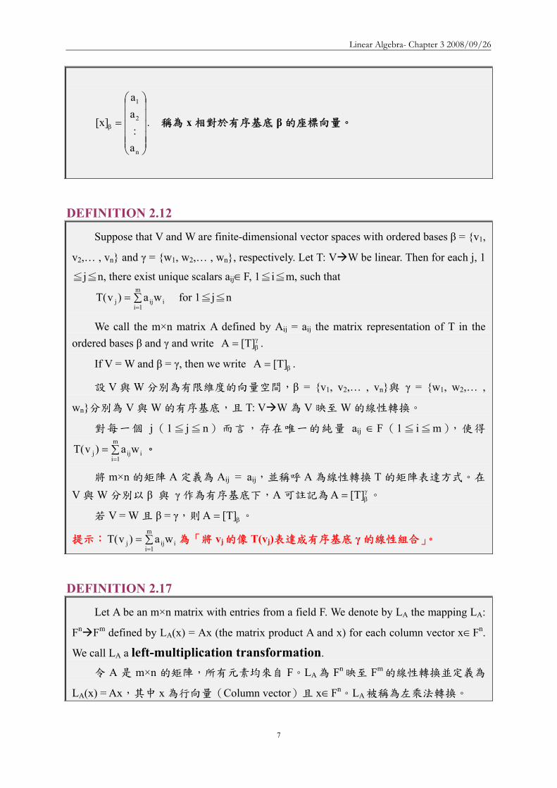
Linear Algebra- Chapter 3 20080926
9
rank(PAQ) = rank(PA) = rank(A)
註Theorem 34 是為後續 Reduced Row Echelon Form of Matrix 做準備一個矩陣經過
基本行運算或基本列運算或基本行與列運算後並不會改變 RANK
Corollary
Elementary row and column operations on a matrix are rank-preserving
矩陣的基本列與行運算不會改變矩陣的 Rank
此推論結果是計算反矩陣解線性方程組的重要依據
Theorem 35 The rank of any matrix equals the maximum number of its linearly independent
columns that is the rank of a matrix is the dimension of the subspace generated by its
column
任一矩陣的 Rank 等於其最大線性獨立行向量數目即矩陣的 Rank 是由矩陣的
行向量生成的子空間的維度【LA Fn Fm】
【Proof】
For any AisinMmtimesn(F)
rank(A) = rank(LA) = dim(R(LA))
Let β be the standard basis of Fn Then β spans Fn and hence by Theorem 22
R(LA ) = span(LA (β)) = span(LA(e1) LA(e2)hellip LA(en))
But for any j we have seen in Theorem 213(b) that LA(ej) = Aej = aj where aj is the
jth column of A Hence R(LA ) = span(a1 a2 an)
Thus rank(A) = rank(LA) = dim(span(a1 a2 an))
對任意矩陣 Arank(A) = rank(LA) = dim(R(LA))
令 β為 Fn 的標準基底且生成 Fn
依據 Theorem 22
LA的值域 Range 可由 LA(β)來生成
R(LA) = span(LA (β)) = span(LA(e1) LA(e2)hellip LA(en))
對任意 j 而言由 Theorem 213(b) 可知 LA(ej) = Aej = aj其中aj 為 A 的第 j
個行(aj 相當於 Theorem 213(b)的 vj 或 Theorem 22 的 T(vj))因此 R(LA) =
Linear Algebra- Chapter 3 20080926
10
span(a1 a2 an)
所以 rank(A) = rank(LA) = dimension of R(LA) = dim(span(a1a2an))
Theorem 22 令 V 與 W 為向量空間且 T V W 為線性轉換若 β = v1 v2hellip vn
是定義域(Domain)V 的基底則 T 的值域 Range R(T)可由 T(β)來生成意即 R(T)
= span(T(β)) = span(T(v1) T(v2)hellip T(vn))
Theorem 213 A 為 mtimesn 的矩陣與 B 為 ntimesp 的矩陣uj 與 vj分別為 AB 與 B 的第 j 行
(1 j p≦ ≦ )則
(a) uj = A vj
(b) vj = B ej where ej is the jth standard vector of Fp
EXAMPLE 1
Let ⎟⎟⎟
⎠
⎞
⎜⎜⎜
⎝
⎛=
101110101
A
Observe that the first and second columns of A are linearly independent and that the
third column is a linear combination of the first two Thus
A 的第一行與第二行是線性獨立第三行則是前兩行的線性組合於是
rank(A) = dim⎟⎟⎟⎟
⎠
⎞
⎜⎜⎜⎜
⎝
⎛
⎟⎟⎟
⎠
⎞
⎜⎜⎜
⎝
⎛
⎪⎭
⎪⎬
⎫
⎟⎟⎟
⎠
⎞
⎜⎜⎜
⎝
⎛
⎪⎩
⎪⎨
⎧
⎟⎟⎟
⎠
⎞
⎜⎜⎜
⎝
⎛
⎟⎟⎟
⎠
⎞
⎜⎜⎜
⎝
⎛
111
010
101
span = 2
A 的第 1 行a1=⎟⎟⎟
⎠
⎞
⎜⎜⎜
⎝
⎛
101第 2 行a2=
⎟⎟⎟
⎠
⎞
⎜⎜⎜
⎝
⎛
010第 3 行a3=
⎟⎟⎟
⎠
⎞
⎜⎜⎜
⎝
⎛
111
In order to compute the rank of a matrix A it is frequently useful to postpone the use of
Theorem 35 until A has been suitable modified by means of appropriate elementary row and
column operations so that the number of linearly independent columns is obvious
為了利用 Theorem 35 求矩陣 A 的 Rank(等於最大線性獨立行向量數目)A 可
先經過基本列或行運算使其線性獨立的行數變得比較明顯
EXAMPLE 2 Let
Linear Algebra- Chapter 3 20080926
11
⎟⎟⎟
⎠
⎞
⎜⎜⎜
⎝
⎛=
211301121
A
If we subtract the first row of A from rows 2 and 3 (type 3 elementary row operations)
the result is
⎟⎟⎟
⎠
⎞
⎜⎜⎜
⎝
⎛
minusminus
110220121
If we now substract twice the first column from the second and substract the first
column from the third (type 3 elementary column operations) we obtain
⎟⎟⎟
⎠
⎞
⎜⎜⎜
⎝
⎛
minusminus
110220001
(後二行線性相依最大線性獨立行數為 2)
It is now obvious that the maximum number of linearly independent column of this matrix is 2 Hence the rank of A is 2
Theorem 36 Let A be an mtimesn matrix of rank r Then r m r n and by means of a finite number ≦ ≦
of elementary row and column operations A can be transformed into the matrix
D = ⎟⎟⎠
⎞⎜⎜⎝
⎛
32
1r
OOOI
where O1 O2 and O3 are zero matrices Thus Dii = 1 for i r and ≦
Dij = 0 otherwise
令 A 為 Rank 等於 r 的 mtimesn 矩陣則 r m≦ 且 r n≦ 經過有限次數的基本行與列
運算讓 A 化成 D = ⎟⎟⎠
⎞⎜⎜⎝
⎛
32
1r
OOOI
其中Ir 為對角元素為 1 的對角矩陣即 A 可經
過有限次數的基本行及列運算取得沿對角線前 r 個位置皆為 1其餘各處皆為 0 的
矩陣 D
【Proof】
If A is the zero matrix r = 0 In this case the conclusion follows with D = A
若 A 為零矩陣則 r = 0 且 D = A
Now suppose that AneO and r = rank(A) then r gt 0
The proof is by mathematical induction on m the number of rows of A
若 A 非零矩陣且 r = rank(A)則 r gt 0
Linear Algebra- Chapter 3 20080926
12
採用數學歸納法
Suppose that m = 1
A can be transformed into the matrix (1 0 hellip0)
So rank(D) = rank(A) = 1 by Corollary to Theorem 34 and Theorem 35 Thus the
theorem is established for m = 1
設 m = 1則 A 可以化成(1 0 hellip0)
依據 Corollary to Theorem 34 及 Theorem 35
rank(D) = rank(A) = 1
故本定理對 m = 1 的矩陣是成立的
Next assume that the theorem holds for any matrix with at most m - 1 row (for some m
gt1)
We must prove that the theorem holds for any matrix with m rows
其次假設本定理對至多含 m - 1 列的矩陣皆成立(m gt 1)
至於含 m 列的矩陣是否成立
If n = 1 Theorem 36 can be established in a manner analogous to that for m = 1
若 n = 1則可按 m = 1 的方式證明本定理對於 n = 1 的矩陣成立
We now suppose that n gt 1 Since A ne O Aijne0 for some i j By means of at most one
elementary row and at most one elementary column operation (each of type 1) We can
move the nonzero entry to the 11 position By means of of at most one additional type 2
operation we can assure a 1 in the 11 position By means of at most m ndash 1 type 3 row
operations and at most n ndash 1 type 3 column operations we can eliminate all nonzero entries
in the first row and the first column with the exception of the 1 in the 11 postion
Thus with a finite number of elementary operation A can be transformed into a
matrix
經過有限次數的基本行及列運算可將 A 轉換成
⎪⎪⎭
⎪⎪⎬
⎫
⎪⎪⎩
⎪⎪⎨
⎧
=
0B
0001
B where Brsquo is an (m-1)times(n-1) matrix
Brsquo has rank one less than B
Brsquo的 Rank 比 B 少 1
Since rank(A) = rank(B) = r rank(Brsquo) = r ndash 1 Therefore r ndash1 ≦ m ndash 1 and r ndash1 ≦
Linear Algebra- Chapter 3 20080926
13
n ndash 1 by the induction hypothesis Hence r ≦ m and r ≦ n
由於 rank(A) = rank(B) = r故 rank(Brsquo) = r ndash 1
依數學歸納法 r ndash1 ≦ m ndash 1 且 r ndash1 ≦ n ndash 1
因此 r ≦ m 且 r ≦ n
Also by the induction hypothesis Brsquo can be transformed by a finite number of
elementary row and column operations into the (m-1)times(n-1) matrix Drsquo such that
同樣地依據數學歸納法Brsquo 可經過有限次數的基本行與列運算轉換成 (m-
1)times(n-1) 的矩陣 Drsquo使得
Dlsquo= ⎟⎟⎠
⎞⎜⎜⎝
⎛ minus
65
41r
OOOI
where O4 O5 and O6 are zero matrices
That is Drsquo consists of all zeros except for its first r-1 diagonal entries which are ones
Let
⎪⎪⎭
⎪⎪⎬
⎫
⎪⎪⎩
⎪⎪⎨
⎧
=
0D
0001
D
We see that the theorem now follows once we show that D can be obtained from B by
means of a finite number of elementary row and column operations
D 可由 B 經過有限次基本行及列運算而取得
Thus since A can be transformed into B and B can be transformed into D each by a
finite number of elementary operations A can be transformed into D by a finite number of
elementary operations
經過有限次基本行及列運算A B D
Finally since Drsquo contains ones as its first r ndash 1 diagonal entries D contains ones as its
first r diagonal entries and zeros elsewhere
最後Drsquo沿對角線前 r-1 個位置皆為 1故 D 沿對角線前 r 個位置皆為 1其餘
各處皆為 0
EXAMPLE 3 Consider the maxtrix
⎟⎟⎟⎟⎟
⎠
⎞
⎜⎜⎜⎜⎜
⎝
⎛
=
192362100280844422420
A
Linear Algebra- Chapter 3 20080926
14
By means of a succession of elementary row and column operations we can transform
A into a matrix D as in Theorem 36
透過一系列的基本行與列運算將 A 轉換成 D
D
00000001000001000001
192362100280844422420
A =
⎟⎟⎟⎟⎟
⎠
⎞
⎜⎜⎜⎜⎜
⎝
⎛
==
⎟⎟⎟⎟⎟
⎠
⎞
⎜⎜⎜⎜⎜
⎝
⎛
=
By the corollary to Theorem 34 rank(A) = rank(D) Clearly however rank(D) = 3 so rank(A) = 3
Corollary 1 Let A be an mtimesn matrix of rank r Then there exist invertible matrices B and C of sizes
mtimesm and ntimesn respectively such that D = BAC where D = ⎟⎟⎠
⎞⎜⎜⎝
⎛
32
1r
OOOI
is the mtimesn matrix
in which O1 O2 and O3 are zero matrices
令 A 為 mtimesn 的矩陣Rank 為 r存在可逆的 mtimesm 矩陣 B 與 ntimesn 矩陣 C使得
D = BAC其中D = ⎟⎟⎠
⎞⎜⎜⎝
⎛
32
1r
OOOI
為 mtimesn 的矩陣O1O2 及 O3 為零矩陣
【Proof】
By Theorem 36 A can be transformed by means of a finite number of elementary
row and column operations into the matrix D
We can appeal to Theorem 31 each time we perform an elementary operation Thus
there exist elementary mtimesm matrices E1 E2hellipEp and elementary ntimesn matrices G1
G2hellipGq such that D = EpEp-1hellipE2E1AG1G2hellipGq
By Theorem 32 each Ej and Gj is invertible Let B = EpEp-1hellipE2E1 and C =
G1G2hellipGq Then B and C are invertible and D = BAC
依據 Theorem 36A 可經過有限次的基本列與行運算化成 D
引用 Theorem 31每一次皆實施某一個基本列運算於是存在基本的 mtimesm 矩
陣 E1 E2hellip Ep 與 基 本 的 ntimesn 矩 陣 G1 G2hellip Gq 使 得 D = EpEp-
1hellipE2E1AG1G2hellipGq
依據 Theorem 32 每一個基本矩陣 Ej與 Gj 皆為可逆令 B = EpEp-1hellipE2E1 與 C =
G1G2hellipGq於是 B 與 C 皆為可逆且 D = EpEp-1hellipE2E1AG1G2hellipGq = BAC
Linear Algebra- Chapter 3 20080926
15
Theorem 31 令 AisinMmtimesn(F)並假設 B 是由 A 經實施某一基本列【或行】運算後所得
到的矩陣則存在一個 mtimesm 【或 ntimesn】基本矩陣 E使得 B = EA【或 B = AE】E
矩陣是由 Im 【或 In】 經實施與「由 A 得到 B」相同的基本列【或行】運算後所得
到的矩陣反之若 E 是一個 mtimesm【或 ntimesn】的基本矩陣則 EA【或 AE】是由 A
經過與「由 Im 【或 In】 得到 E」相同的基本列【或行】運算後所得到的矩陣
Theorem 32 基本矩陣為可逆矩陣且基本矩陣的反矩陣亦是同一型的基本矩陣
Theorem 36 令 A 為 Rank 等於 r 的 mtimesn 矩陣則 r m≦ 且 r n≦ 經過有限次數的基
本行與列運算讓 A 化成 D = ⎟⎟⎠
⎞⎜⎜⎝
⎛
32
1r
OOOI
其中Ir為對角元素為 1 的對角矩陣
Corollary 2 Let A be an mtimesn matrix Then
(a) rank(At) = rank(A)
矩陣轉置後的 RANK 不變
(b) The rank of any matrix equals the maximum number of its linearly independent
rows that is the rank of a matrix is the dimension of the subspace generated by
rows
任一矩陣的 Rank 等於最大線性獨立列向量的數目即矩陣的 Rank 等於由該
矩陣列向量所生成的子空間的維度
(c) The rows and columns of any matrix generate subspaces of the same dimension
numerically equal to the rank of the matrix
任一矩陣的列向量與行向量生成的子空間的維度相同維度等於該矩陣的
Rank
【Proof】
By Corollary 1 there exist invertible matrices B and C such that D = BAC where D
satisfies the stated conditions of the corollary Taking transposes we have
Dt = (BAC) t = CtAtBt
Since B and C are invertible so are Bt and Ct
Hence by Theorem 34 rank(At) = rank(CtAtBt) = rank(Dt)
Suppose that r = rank(A)
Then Dt is an ntimesm matrix with the form of the matrix D in Corollary 1 and hence
Linear Algebra- Chapter 3 20080926
16
rank(Dt) = r by Theorem 35
Thus
rank(At) = rank(Dt) = r = rank(A)
依據 Corollary 1存在可逆矩陣 B 與 C使得 D = BAC
取其轉置可得Dt = (BAC) t = CtAtBt
由於 B 與 C 為可逆故 Bt 與 Ct 亦為可逆
依據 Theorem 34得知 rank(At) = rank(CtAtBt) = rank(Dt)
設 r = rank(A)
則 Dt為一 ntimesm 的矩陣型式與 D 相同(參考 Corollary 1)
且依據 Theorem 35 得知 rank(Dt) = r
於是 rank(At) = rank(Dt) = r = rank(A)
Theorem 34 Let A be an mtimesn matrix If P and Q are invertible mtimesm and ntimesn matrices
respectively then 令 A 為 mtimesn 的矩陣若 P 與 Q 分別為可逆的 mtimesm 與 ntimesn 矩陣
則
(a) rank(AQ) = rank(A)
(b) rank(PA) = rank(A)
(c) rank(PAQ) = rank(A)
Theorem 35 The rank of any matrix equals the maximum number of its linearly
independent columns that is the rank of a matrix is the dimension of the subspace
generated by its column 任一矩陣的 Rank 等於其最大線性獨立行向量數目即矩陣
的 Rank 是由矩陣的行向量生成的子空間的維度【LA Fn Fm】
Corollary 3 Every invertible matrix is a product of elementary matrices
每一可逆矩陣均可為基本矩陣的乘積
【Proof】
If A is an invertible ntimesn matrix then rank(A) = n Hence the matrix D in Corollary 1
equals In and there exist invertible matrices B and C such that In = BAC
As in the proof of Corollary 1 note that B = EpEp-1hellipE2E1 and C = G1G2hellipGq where
the Eirsquos and Girsquos are elementary matrices Thus A = B-1InC-1 = B-1C-1 so that
A = E1-1E2
-1hellipEp-1Gq
-1Gq-1-1hellipG1
-1
Linear Algebra- Chapter 3 20080926
17
The inverses of elementary matrices are elementary matrices however and hence A is
the product of elementary matrices
若 A 為可逆的 ntimesn 矩陣則 rank(A) = n
因此 Corollary 1 中的矩陣 D 為 In且存在可逆的 B 與 C 矩陣使得 In = BAC
如同 Corollary 1 的證明一樣B = EpEp-1hellipE2E1 且 C = G1G2hellipGq其中Eirsquos 與
Girsquos 皆為基本矩陣
於是A = B-1InC-1 = B-1C-1即 A = E1-1E2
-1hellipEp-1Gq
-1Gq-1-1hellipG1
-1
基本矩陣的反矩陣亦為基本矩陣A 是基本矩陣的乘積
Theorem 37 Let T V W and U W Z be linear transformations on finite-dimensional vector
spaces V W and Z and let A and B be matrices such that the product AB is defined Then
令 VW 與 Z 為有限維度的向量空間T V W 與 U W Z 為線性轉換且
A 與 B 為滿足乘積 AB 定義的矩陣則
(a) rank(UT) ≦ rank(U)
(b) rank(UT) ≦ rank(T)
(c) rank(AB) ≦ rank(A)
(d) rank(AB) ≦ rank(B)
【Proof】
(a) Clearly R(T)subeW
Hence R(UT) = UT(V) = U(R(T)) sube U(W) = R(U)
Thus rank(UT) = dim(R(UT)) ≦ dim (R(U)) = rank(U)
(c) By (a) rank(AB) = rank(LAB) = rank (LALB) ≦ rank(LA) = rank(A)
(d) By (c) and Corollary 2 to Theorem 36
rank(AB) = rank((AB)t) = rank(B t A t) ≦ rank(B t) = rank (B) (b) Let α β and γ be ordered bases for V W and Z respectively and let Arsquo = γ
β]U[
and Brsquo = βα]T[ Then ArsquoBrsquo = γ
α]UT[ by Theorem 211
Hence by Theorem 33 and (d)
rank(UT) = rank(ArsquoBrsquo) ≦ rank(Brsquo) = rank (T)
Theorem 211 Let V W and Z be finite-dimensional vector space with ordered bases α β
and γ respectively Let T V W and U W Z be linear transformation Then
Linear Algebra- Chapter 3 20080926
18
βα
γβ
γα = [T][U][UT] 令 VW 與 Z 是有限維度的向量空間αβ 與 γ 分別為 VW 與
Z 的有序基底令 T V W (先 α β) 且 U W Z (後 β γ)則 βα
γβ
γα = [T][U][UT]
Theorem 33 Let T V W be a linear transformation between finite dimensional vector
spaces and let β and γ be ordered bases for V and W respective Then rank(T) = rank( γ
β[T] ) 令 T V W且 β 與 γ 分別為有限維度向量空間 V 與 W 的有序基底
則 rank(T) = rank( γβ[T] )
EXAMPLE 4
(a) Let ⎟⎟⎠
⎞⎜⎜⎝
⎛minus
=11111121
A (第一列與第二列是 LI) rank(A) = 2
(b) Let ⎟⎟⎟
⎠
⎞
⎜⎜⎜
⎝
⎛=
003011011131
A (第三列與第一二列是 LD)rank(A) = 2
(c) Let ⎟⎟⎟
⎠
⎞
⎜⎜⎜
⎝
⎛
minus=
011111121321
A (三列為 LI) rank(A) = 3
The inverse of a Matrix
We have remarked that an ntimesn matrix is invertible if and only if its rank is n Since we
know how to compute the rank of any matrix we can always test a matrix to determine
whether it is invertible We now provide a simple technique for computing the inverse of a
matrix that utilizes elementary row operations
已知 ntimesn 矩陣為可逆的『若且唯若』條件為該矩陣的 Rank 等於 n
DEFINITION 34 Augmented Matrix Let A and B be mtimesn and mtimesp matrices respectively By the augmented matrix )BA(
we mean that the mtimes(n+p) matrix )BA( that is the matrix whose first n columns are the
columns of A and whose last p columns are the columns of B 設 A 與 B 分別為 mtimesn 與 mtimesp 的矩陣則增廣矩陣(Augmented matrix) )BA(
Linear Algebra- Chapter 3 20080926
19
為一 mtimes(n+p)的矩陣 )BA( 該矩陣的前 n 行(Column)為 A 的所有的行後 p
行為 B 的所有行
Let A be an invertible ntimesn matrix and consider the ntimes2n augmented matrix C= )IA( n
C= )IA( n )AI()IAAA(CA 1
nn111 minusminusminusminus ==
By Corollary 3 to Theorem 36 A-1 is the product of elementary matrices say
A = EpEp-1hellipE2E1 (A-1 是多個基本矩陣的乘積)
Thus )AI()IAAA(CA 1
nn111 minusminusminusminus == )AI(CA)IA(EEE 1
n1
n11ppminusminus
minus ==
We have the following result If A is an invertible invertible ntimesn matrix then it is
possible to transform the matrix (AIn) into the matrix (InA-1) by means of a finite
number of elementary row operations
若 A 為一可逆的 ntimesn 矩陣則可經過有限次數的基本列運算將矩陣 (AIn) 化成
(InA-1)
Conversely suppose that A is invertible and that for some ntimesn matrix B the matrix
(AIn) can be transformed into the matrix (InB) by a finite number of elementary row
operations Let E1 E2hellip Ep be the elementary matrices associated with these elementary row
operations as in Theorem 31 then
反之假設 A 是可逆且矩陣(AIn)可經有限次數的基本列運算轉換成矩陣(InB)
並令 E1 E2hellip Ep 分別為 Theorem 31 所稱的基本矩陣則
)BI()IA(EEE nn11pp =minus
Let M = EpEp-1hellipE2E1 we have 令 M = EpEp-1hellipE2E1
)BI()IA(EEE nn11pp =minus )BI()IA(M)MMA( nn ==
Linear Algebra- Chapter 3 20080926
20
Hence MA = In and M = B It follows that M = A-1 So B = A-1
可由 MA = In 及 M = B 得知M 就是 A-1故 B 就是 A-1
Thus we have the follow resultsIf A is an invertible ntimesn matrix and the matrix
(AIn) is transformed in a matrix of the form (InB) by means of a finite number of
elementary row operations then B=A-1
若 A 為一可逆的 ntimesn 矩陣且矩陣 (AIn) 可經有限次數的基本列運算化成
(InB)則 B=A-1
If on the other hand A is an ntimesn matrix that is not invertible then rank(A) lt n Hence
any attempt to transform (AIn) into a matrix of the form (InB) by means of elementary row
operations must fail
反之若 A 是一不可逆的 ntimesn 矩陣則 rank(A) lt n因此任何想利用基本列運算
要將矩陣 (AIn) 化成 (InB)的努力必定失敗
Thus we have the follow results If A is an notinvertible ntimesn matrix then any attempt
to transform (AIn) into a matrix of the form (InB) produce a row whose first n entries
are zeros
若 A 是一不可逆的 ntimesn 矩陣任何想將矩陣 (AIn) 化成 (InB)的努力最後會
產生一前 n 個元素均為 0 的列
EXAMPLE 5
We determine whether the matrix ⎟⎟⎟
⎠
⎞
⎜⎜⎜
⎝
⎛=
133242420
A is invertible and if it is we
compute its inverse
A 是否為可逆矩陣
We attempt to use elementary row operations to transfer
Linear Algebra- Chapter 3 20080926
21
⎟⎟⎟
⎠
⎞
⎜⎜⎜
⎝
⎛=
100010001
133242420
)IA( into a matrix of the form (InB)
看看能否利用基本行與列運算將矩陣 (AIn) 化成 (InB)
Interchanging rows 1 and 2
⎟⎟⎟
⎠
⎞
⎜⎜⎜
⎝
⎛
100001010
133420242
Multiplying the first row by 12
⎟⎟⎟
⎠
⎞
⎜⎜⎜
⎝
⎛
10000100
133420121 2
1
Adding -3 times row 1 to row 3
⎟⎟⎟
⎠
⎞
⎜⎜⎜
⎝
⎛
minusminusminus 1000100
230420121
23
21
Multiplying row 2 by 12 to obtain 1 in the 22 position
⎟⎟⎟
⎠
⎞
⎜⎜⎜
⎝
⎛
minus
minus
minusminus 100000
230210121
23
21
21
Adding -2 times row 2 to row 1 and 3 times row 2 to row 3
⎟⎟⎟
⎠
⎞
⎜⎜⎜
⎝
⎛
minus
minusminus
10001
400210301
23
2321
21
Multiplying row 3 by 14
⎟⎟⎟
⎠
⎞
⎜⎜⎜
⎝
⎛
minus
minusminus
41
83
8321
21
0001
100210301
Adding appropriate multiply of row 3 to row 1 and 2 completes the process
⎟⎟⎟
⎠
⎞
⎜⎜⎜
⎝
⎛
minusminus
minus
41
83
83
21
43
41
43
85
81
100010001
目標達成
Thus A is invertible and ⎟⎟⎟
⎠
⎞
⎜⎜⎜
⎝
⎛
+minus+minus+minus+minus+
=minus
41
83
83
21
43
41
43
85
81
1A
Linear Algebra- Chapter 3 20080926
22
EXAMPLE 6
We determine whether the matrix ⎟⎟⎟
⎠
⎞
⎜⎜⎜
⎝
⎛minus=451112
121A is invertible and if it is we
compute its inverse
A 是否為可逆矩陣
We attempt to use elementary row operations to transfer
⎟⎟⎟
⎠
⎞
⎜⎜⎜
⎝
⎛minus=
100010001
451112
121)IA( into a matrix of the form (InB)
看看能否利用基本行與列運算將矩陣 (AIn) 化成 (InB)
Adding -2 times row 1 to row 2 and -1 times row 1 to row 3 then addig row 2 to row
3
⎟⎟⎟
⎠
⎞
⎜⎜⎜
⎝
⎛minus
100010001
451112
121
⎟⎟⎟
⎠
⎞
⎜⎜⎜
⎝
⎛
minusminusminusminus
101012001
330330
121
⎟⎟⎟
⎠
⎞
⎜⎜⎜
⎝
⎛
minusminusminusminus
113012001
000330
121
is a matrix with row whose first 3 entries are zeros Therefore A is not invertible
最後一列前 3 個元素均為 0
EXAMPLE 7 Let T P2(R) P2(R) be defined by T(f(x)) = f(x)+frsquo(x)+frdquo(x) where frsquo(x) and frdquo(x)
denote the first and second derivatives of f(x) We use Corollary 1 to Theorem 218 to test
T for invertibility and compute the inverse if T is invertible Taking β=1 x x2 to be the
standard ordered basis of P2(R) we have
令 T P2(R) P2(R) 為線性轉換且定義為 T(f(x)) = f(x)+frsquo(x)+frdquo(x)利用
Corollary 1 to Theorem 218 來測試 T 是否可逆並計算其逆轉換取 β=1 x x2為
P2(R)的標準有序基底
T(1) = 1 = 1bull1+0bullx+0bullx2
T(x) = 1+x = 1bull1+1bullx+0bullx2
Linear Algebra- Chapter 3 20080926
23
T(x2) = 2+2x+x2 = 2bull1+2bullx+1bullx2
⎟⎟⎟
⎠
⎞
⎜⎜⎜
⎝
⎛=β
100210211
[T] 稱為 T 相對有序基底 β的座標向量
依據 Corollary 1 to Theorem 218 T 可逆『若且唯若』 β[T] 可逆且
1-1 )[T](][T minusββ =
Using the method of Examples 5 and 6 we can show that β[T] is invertible with
inverse
⎟⎟⎟
⎠
⎞
⎜⎜⎜
⎝
⎛minus
minus=minus
β
100210
011)([T] 1
Thus T is is invertible and βminusminus
β = ][T)([T] 11 Hence by Theorem 214 we have
⎟⎟⎟
⎠
⎞
⎜⎜⎜
⎝
⎛minusminus
=⎟⎟⎟
⎠
⎞
⎜⎜⎜
⎝
⎛
⎟⎟⎟
⎠
⎞
⎜⎜⎜
⎝
⎛minus
minus=++ β
minus
2
21
10
2
1
02
2101
aa2aaa
aaa
100210
011)]xaxa(a[T
Therefore T-1(a0+a1x+a2x2) = (a0-a1)+(a1-2a2)x+a2x2 Corollary 1 to Theorem 218 Let V be finite-dimensional vector space with an ordered basis β and let T V V be linear Then T is invertible if and only if β[T] is invertible
Furthermore 1-1 )[T](][T minusββ = V 為有限維度的向量空間β 是 V 的有序基底令 T
V V 為線性轉換 T 為可逆的『若且唯若』條件為 β[T] 可逆再者
1-1 )[T](][T minusββ =
Theorem 214 Let V and W be finite-dimensional vector spaces having ordered bases β and γ respectively and let T V W be linear Then for each uisinV we have β
γβγ = [u][T][T(u)]
V 與 W 為有限維度的向量空間β 與 γ分別 V 與 W 的有序基底令 T V W 為線
性轉換則 V 中的 u 映至 W 的結果 T(u) 相對於有序基底 γ 的座標向量為
βγβγ = [u][T][T(u)]
Invertible and Inverse of MATRIX Let A be an n times n matrix If a matrix B can be found such that AB = BA = In then A is
Linear Algebra- Chapter 3 20080926
24
said to be invertible and B is called the inverse of A (denote B = A-1 and A-k=(A-1)k )
If such a matrix B does not exist then A has no inverse
EXAMPLE
⎥⎦
⎤⎢⎣
⎡=
4321
A and ⎥⎦
⎤⎢⎣
⎡minus
minus=
21
23
12B
221
23
221
23
I1001
432112
BA
I100112
4321
AB
=⎥⎦
⎤⎢⎣
⎡=⎥
⎦
⎤⎢⎣
⎡⎥⎦
⎤⎢⎣
⎡minus
minus=
=⎥⎦
⎤⎢⎣
⎡=⎥
⎦
⎤⎢⎣
⎡minus
minus⎥⎦
⎤⎢⎣
⎡=
Thus AB = BA = I2 proving that the matrix A has inverse B
Theorem The inverse of an invertible matrix is unique
Let B and C be inverse of A
Thus AB = BA = In and AC = CA = In
Multiply both sides of the equation AB = In by C
C(AB) = CIn (CA)B = C
InB = C B = C
Thus an invertible matrix has only one inverse
How to find AHow to find A--11
Based on the GaussBased on the Gauss--Jordan algorithmJordan algorithmLet A be an invertible matrix Then AALet A be an invertible matrix Then AA--11=I=Inn
Let the columns of Let the columns of AA--11 be be XX11 XX22 helliphellip XXnn and the columns of I and the columns of Inn be be CC11CC22helliphellipCCnn
Find AFind A--11 by finding by finding XX11 XX22 helliphellip XXnn Write the equation AAWrite the equation AA--11=I=Inn in the formin the form
[ ] [ ]n21nn211 CCCI XXXALet LL ==minus
[ ] [ ][ ] [ ]n21n21
n21n21
CCCAXAXXACCCXXXALL
LL
=rArr=
nn2211 CAXCAX CAX === LThus
How to find AHow to find A--11
Solving these systems by using Gauss-Jordan elimination on the large augmented matrix [AC1 C2hellipCn]
Thus when A-1 exits
[ ] [ ] [ ] 1n
1nn ABwhereBIAIIA minusminus ==asympasympL
If the reduced echelon form of [If the reduced echelon form of [AIAInn] is computed and ] is computed and the first part is not of the form Ithe first part is not of the form Inn then A has no inversethen A has no inverse
[ ][ ]n21n
n21
XXXI CCCAmatrix augmented
LL
L
asympasymp
Linear Algebra- Chapter 3 20080926
25
Example Example 1212
⎥⎥⎥
⎦
⎤
⎢⎢⎢
⎣
⎡
minusminusminusminusminus
=100531010532001211
]IA[ 3
⎥⎥⎦
⎤
⎢⎢⎣
⎡minusminusminus
minusminus
+minus+
asymp
101320012110001211
1RR1R3
2)(R2
⎥⎥⎦
⎤
⎢⎢⎣
⎡minus
minusminusminusasymp
101320012110001211
R2)1(
⎥⎥⎥
⎦
⎤
⎢⎢⎢
⎣
⎡
minusminusminusminusminus
=531532211
ADetermine the inverse of
Example Example 2222
⎥⎥⎦
⎤
⎢⎢⎣
⎡
minusminusminusminus
minus++asymp
123100012110013101
R2)2(R3R2R1
⎥⎥⎦
⎤
⎢⎢⎣
⎡
minusminusminus
minus++asymp
123100135010010001
R3)1(R2R3R1
123135110
A 1
⎥⎥⎥
⎦
⎤
⎢⎢⎢
⎣
⎡
minusminusminus=minus
⎥⎥⎦
⎤
⎢⎢⎣
⎡
minusminus
minus
+minus+asymp
135000011210012301
3R2R3R2)1(R1
ExampleExampleDetermine the inverse of
⎥⎥⎦
⎤
⎢⎢⎣
⎡
minus=
412721511
A
⎥⎥⎦
⎤
⎢⎢⎣
⎡
minus=
100412010721001511
][ 3IA
⎥⎥⎦
⎤
⎢⎢⎣
⎡
minusminusminusminus
minus+minus+asymp
102630011210001511
R1)2(R31)R1(R2
There is no need to proceed further There is no need to proceed further The reduced echelon form cannot have a one in the (3 3) locatioThe reduced echelon form cannot have a one in the (3 3) location n
The reduced echelon form cannot be of the form [IThe reduced echelon form cannot be of the form [Inn B] B] Thus Thus AAndashndash11 does not existdoes not exist
Properties of Matrix InverseProperties of Matrix Inverse
Let Let AA and and BB be invertible matrices andbe invertible matrices and cc a nonzero scalar a nonzero scalar ThenThen
AA =minusminus 11)( 111 1)( 2 minusminus = A
ccA
111)( 3 minusminusminus = ABAB
nn AA )()( 4 11 minusminus =tt AA )()( 5 11 minusminus =
Color Models Color Models 1212
A color model in the context of graphics is a method of A color model in the context of graphics is a method of implementing colorsimplementing colorsThe common used models include RGB model and YIQ modelThe common used models include RGB model and YIQ modelThe RGB model is used in computer monitors and the YIQ model The RGB model is used in computer monitors and the YIQ model is used in television screensis used in television screensAn RGB computer signal can be converted to a YIQ television An RGB computer signal can be converted to a YIQ television signal using the matrix transformationsignal using the matrix transformation
⎥⎥⎥
⎦
⎤
⎢⎢⎢
⎣
⎡
⎥⎥⎥
⎦
⎤
⎢⎢⎢
⎣
⎡
minusminusminus=
⎥⎥⎥
⎦
⎤
⎢⎢⎢
⎣
⎡
BGR
311523212321275596
114587299
QIY
YIQgtRGBYIQgtRGB
Color Models Color Models 2222
A signal is converted from a television screen to a computer monA signal is converted from a television screen to a computer monitor itor using inverse of the above matrixusing inverse of the above matrix
⎥⎥⎥
⎦
⎤
⎢⎢⎢
⎣
⎡
⎥⎥⎥
⎦
⎤
⎢⎢⎢
⎣
⎡
minusminusminus=
⎥⎥⎥
⎦
⎤
⎢⎢⎢
⎣
⎡rArr
⎥⎥⎥
⎦
⎤
⎢⎢⎢
⎣
⎡
⎥⎥⎥
⎦
⎤
⎢⎢⎢
⎣
⎡
minusminusminus=
⎥⎥⎥
⎦
⎤
⎢⎢⎢
⎣
⎡minus
QIY
0751108116472721
6209561
BGR
QIY
311523212321275596
114587299
BGR 1
CryptographyCryptography 密碼學密碼學 1212
Cryptography is the process of coding and decoding messagesCryptography is the process of coding and decoding messagesThe technique can be traced back to the ancient Greeks Today The technique can be traced back to the ancient Greeks Today governments use sophisticated methods of coding and decoding governments use sophisticated methods of coding and decoding messagesmessagesOne type of code that is extremely difficult to break makes use One type of code that is extremely difficult to break makes use of a of a large matrix to encode a message large matrix to encode a message The receiver of the message decodes it using the inverse of the The receiver of the message decodes it using the inverse of the matrixmatrixThe first matrix is called the encoding matrix and its inverse The first matrix is called the encoding matrix and its inverse is is called the decoding matrixcalled the decoding matrix
Cryptography Cryptography 密碼學密碼學 2222
A A-1Message
Encoding MatrixEncoding Matrix
Decoded MessageTransmission
Decoding MatrixDecoding Matrix
Linear Algebra- Chapter 3 20080926
26
Example Example 1212
Let the message be Let the message be BUY IBM STOCKBUY IBM STOCKAnd the encoding matrix beAnd the encoding matrix be
⎥⎥⎥
⎦
⎤
⎢⎢⎢
⎣
⎡ minusminusminus
434110433
B U Y B U Y -- I B M I B M -- S T O C KS T O C K2 21 25 27 9 2 13 27 19 20 15 3 112 21 25 27 9 2 13 27 19 20 15 3 11
⎥⎥⎥
⎦
⎤
⎢⎢⎢
⎣
⎡ minusminusminusminusminus=
⎥⎥⎥
⎦
⎤
⎢⎢⎢
⎣
⎡
⎥⎥⎥
⎦
⎤
⎢⎢⎢
⎣
⎡ minusminusminus
2331372091431715418461146
222117196116169
27319225271527921112013272
434110433
EncodingEncoding
Example Example 2222
Let the message be Let the message be BUY IBM STOCKBUY IBM STOCKAnd the decoding matrix beAnd the decoding matrix be
⎥⎥⎥
⎦
⎤
⎢⎢⎢
⎣
⎡
minusminus 334344101
B U Y B U Y -- I B M I B M -- S T O C KS T O C K2 21 25 27 9 2 13 27 19 20 15 3 112 21 25 27 9 2 13 27 19 20 15 3 11
⎥⎥⎥
⎦
⎤
⎢⎢⎢
⎣
⎡=
⎥⎥⎥
⎦
⎤
⎢⎢⎢
⎣
⎡ minusminusminusminusminus
⎥⎥⎥
⎦
⎤
⎢⎢⎢
⎣
⎡
minusminus 27319225271527921112013272
2331372091431715418461146
222117196116169
334344101
DecodingDecoding
3-3 Systems of Linear Equations ndash Theoretical Aspects
The system of equations
mnmn22m11m
2nn2222121
1nn1212111
bxaxaxa
bxaxaxabxaxaxa
=+++
=+++=+++
(S)
were aij and bi (1≦i≦m and 1≦j≦n) are scalars in a field F and x1 x2hellipxn are n
variables taking values in F is called a system of m linear equations in n unknows over the
field F
上式稱為佈於 Field F 含有 n 個未知數m 個線性方程式的系統或方程組(system
of m linear equations in n unknows)
The mtimesn matrix
⎟⎟⎟⎟⎟
⎠
⎞
⎜⎜⎜⎜⎜
⎝
⎛
=
mn2m1m
n22221
n11211
aaa
aaaaaa
A is called the coefficient matrix of the
system (S)(係數矩陣) If we let
⎟⎟⎟⎟⎟
⎠
⎞
⎜⎜⎜⎜⎜
⎝
⎛
=
n
2
1
x
xx
x and
⎟⎟⎟⎟⎟
⎠
⎞
⎜⎜⎜⎜⎜
⎝
⎛
=
m
2
1
b
bb
b Then the system (S) may
be rewritten as a single matrix equation Ax = b(單一矩陣方程式)
To exploit the results that we have developed we often consider a system of linear
equations as a single matrix equation
Linear Algebra- Chapter 3 20080926
27
A solution to the system (S) is an n-tuple n
n
2
1
F
s
ss
s isin
⎟⎟⎟⎟⎟
⎠
⎞
⎜⎜⎜⎜⎜
⎝
⎛
= such that As = b The set of
all solutions to the system (S) is called the solution set of the system(解集合) System (S)
is called consistent(相容) if its solution set is nonempty otherwise it is called
inconsistent(不相容)
方程組(S)的解為一 n 序組該序組可以使 As = b方程組的所有解所成的集合
稱為該方程組的解集合(Solution set)方程組的解集合非空集合者稱為「相容」解
集合空集合者稱為「不相容」
EXAMPLE 1
Consider 6x2xx1xx3x2
321
321
=+minus=++
that is ⎟⎟⎠
⎞⎜⎜⎝
⎛=
⎟⎟⎟
⎠
⎞
⎜⎜⎜
⎝
⎛
⎟⎟⎠
⎞⎜⎜⎝
⎛minus 6
1
xxx
211132
3
2
1
(以矩陣表示)
This system has many solutions such as ⎟⎟⎟
⎠
⎞
⎜⎜⎜
⎝
⎛minus=
726
s and ⎟⎟⎟
⎠
⎞
⎜⎜⎜
⎝
⎛
minusminus=
34
8s
Consider 1xx0xx
21
21
=+=+
that is ⎟⎟⎠
⎞⎜⎜⎝
⎛=⎟⎟
⎠
⎞⎜⎜⎝
⎛⎥⎦
⎤⎢⎣
⎡10
xx
1111
2
1
顯然地方程組無解
We begin our study of system of linear equations by examining the class of
homogeneous system of linear equations 先討論齊次方程組
DEFINITION 35 Homogeneous amp Nonhomogeneous
A system Ax=b of m linear equations in n unknowns is said to be homogeneous if b=0
Otherwise the system is said to be nonhomogeneous
方程組 Ax = bb = 0 稱為齊次方程組否則稱為非齊次方程組
Any homogeneous system has at least one solution namely the zero vector The next
result gives further information about the set of solutions to a homogeneous system
Linear Algebra- Chapter 3 20080926
28
齊次方程組至少有一個解那就是『零向量』
Theorem 38 Let Ax = 0 be a homogeneous system of m linear equations in n unknowns over a field
F Let K denote the set of all solutions to Ax = 0 Then K = N(LA) hence K is a subspace
of Fn of dimension n - rank(LA) = n- rank(A)
令 Ax = 0 代表一佈於 Field 含有 n 個未知數m 個線性方程式的方程組若令
K 代表該方程組的解集合(Solution set)則 K = N(LA)K 為 Fn 內的子空間且其維
度為 n ndash rank (LA) = n - rank(A)
【Proof】
Clearly K = sisinFn As = 0 = N(LA) The second part now follows from the
dimension theorem
Nullity(T)+rank(T) = dim(V)
Nullity (LA) = dim (Fn) ndashrank (LA ) = n ndash rank (A)
DEFINTION 27 Let V and W be vector space and let T V W be linear We define
the null space (or kernel) N(T) of T to be the set of all vectors x in V such that T(x) = 0
that is N(T) = xisinV T(x) = 0 V 與 W 為向量空間且 T V W 為線性轉換定義
線性轉換 T 的 Null space 為 V 內所有滿足 T(x) = 0 的向量 x 所形成的集合註記為
N(T)Null space 的元素 x 經線性轉換 T 轉換後所對應的「像」為 0意即 T(x) = 0
Null space 內的元素的「像」皆為 0
DEFINITION 217 Let A be an mtimesn matrix with entries from a field F We denote by LA
the mapping LA Fn Fm defined by LA(x) = Ax (the matrix product A and x) for each
column vector xisinFn We call LA a left-multiplication transformation 令 A 是 mtimesn
的矩陣所有元素均來自 FLA 為 Fn 映至 Fm的線性轉換並定義為 LA(x) = Ax其中
x 為行向量(Column vector)且 xisinFnLA被稱為左乘法轉換
Theorem 23 (Dimension Theorem) Let V and W be vector spaces and let T V W be
linear If V is finite-dimensional then Nullity(T) + rank(T) = dim(V) T 的核次數
(Nullity)與秩(Rank)的和等於定義域的維度 dim(V)
Corollary Let Ax = 0 be a homogeneous system of m linear equations in n unknowns over a field
Linear Algebra- Chapter 3 20080926
29
F If m lt n the system Ax = 0 has a nonzero solution
令 Ax = 0 代表一佈於 Field 含有 n 個未知數m 個線性方程式的方程組若 m
lt n則該方程組具有一非零解
【Proof】
Suppose that m lt n Then rank(A) = rank (LA)≦m Hence dim(K) = n - rank(LA) ≧
n ndash m gt 0 where K = N(LA) Since dim(K) gt 0 Kne 0 Thus there exists a nonzero
vector sisinK so s is a nonzero solution to Ax = 0
設 m lt n則 rank(A) = rank (LA) ≦ m依據 Theorem 38K = sisinFn As = 0
= N(LA) = dim(K) = n - rank(LA) ≧ n ndash m gt 0表示 dim(K) gt 0Kne 0故存在非
零向量 s使得 Ax = 0
EXAMPLE 2
Consider 0xxx
0xx2x
321
321
=minusminus=++
Let ⎟⎟⎠
⎞⎜⎜⎝
⎛minusminus
=111
121A be the coefficient matrix of this system It is clear that rank(A)
= 2 If K is the solution set of this system then dim(K) = 3-2 = 1 Thus any nonzero
solution constitutes a basis for K
若 K 是方程組的解所組成的集合(簡稱為解集合)依 Theorem 38 得知 dim(K)
= 3 - 2 = 1因此任一非零解將形成 K 的基底
For example since ⎟⎟⎟
⎠
⎞
⎜⎜⎜
⎝
⎛minus32
1 is a solution to the given system
⎪⎭
⎪⎬
⎫
⎪⎩
⎪⎨
⎧
⎟⎟⎟
⎠
⎞
⎜⎜⎜
⎝
⎛minus32
1 is a basis for
K Thus any vector in K is of the form ⎟⎟⎟
⎠
⎞
⎜⎜⎜
⎝
⎛minus=
⎟⎟⎟
⎠
⎞
⎜⎜⎜
⎝
⎛minus
t3t2
t
32
1t where tisinR
例如因⎟⎟⎟
⎠
⎞
⎜⎜⎜
⎝
⎛minus32
1是方程組的一個解故
⎪⎭
⎪⎬
⎫
⎪⎩
⎪⎨
⎧
⎟⎟⎟
⎠
⎞
⎜⎜⎜
⎝
⎛minus32
1 為 K 的基底K 內的任一向量均
具有如下形式
⎟⎟⎟
⎠
⎞
⎜⎜⎜
⎝
⎛minus=
⎟⎟⎟
⎠
⎞
⎜⎜⎜
⎝
⎛minus
t3t2
t
32
1t
Linear Algebra- Chapter 3 20080926
30
We now turn to the study of nonhomogeneous systems Our next result shows that the
solution set of a nonhomogeneous system Ax = b can be described in terms of the solution of
the homogeneous system Ax = 0 We refer to the equation Ax = 0 as the homogeneous system
corresponding to Ax = b
以下將進一步探討「非齊次方程組」非齊次方程組 Ax = b 的解集合可利用齊次方
程組 Ax = 0 的解來加以說明因此我們可將 Ax = 0 視為 Ax = b 的齊次方程組
Theorem 39 Let K be the solution set of a system of linear equations Ax = b and let KH be the
solution set of the corresponding homogeneous system Ax = 0 Then for any solution s to
Ax = b K =s + KH = s+k kisinKH
設 K 為線性方程組 Ax = b 的解集合且 KH為對應的齊次方程組的解集合則
對 Ax = b 的任一個解 s 而言K =s + KH = s+k kisinKH
【Proof】
Let s be any solution to Ax = b
We must show that K =s + KH
If wisinK then Aw = b Hence
A(w - s) = Aw ndash As = b ndash b = 0
So w - sisinKH
Thus there exists kisinKH such that w - s = k
It follows that w = s + k isin s +KH and therefore Ksube s +KH
Conversely suppose that wisins +KH then w = s + k for some kisinKH
But then Aw = A(s + k) = As + Ak = b + 0 = b so wisinK
Therefore s +KHsubeK and thus K=s +KH
令 s 為 Ax = b 的任一個解我們必須證明「K =s + KH」
若 wisinK則 Aw = b(即 w 為 Ax = b 的解)
於是 A(w - s) = Aw ndash As = b ndash b = 0
所以 w - sisinKH(即 w-s 為 Ax = 0 的解)
w - s 既然是 KH的元素表示有一元素 kisinKH使得 w - s = kw = s + k
w = s + kisins +KH
Linear Algebra- Chapter 3 20080926
31
因此 Ksube s +KH
反之假設 wisins +KH則 KH中存在一元素 k(kisinKH)使得 w = s + k
因 Aw = A(s + k) = As + Ak = b + 0 = b
故 wisinK 是 Ax = b 的解
因此s +KHsubeK
總結K=s +KH
EXAMPLE 3
Consider 4xxx7xx2x
321
321
minus=minusminus=++
The corresponding homogeneous system is the system in Example 2 It is easily
verified that ⎟⎟⎟
⎠
⎞
⎜⎜⎜
⎝
⎛=
411
s is a solution to the preceeding nonhomogeneous system So the
solution set of the system is ⎪⎭
⎪⎬
⎫
⎪⎩
⎪⎨
⎧isin
⎟⎟⎟
⎠
⎞
⎜⎜⎜
⎝
⎛minus+
⎟⎟⎟
⎠
⎞
⎜⎜⎜
⎝
⎛= Rt
32
1t
411
K by Theorem 39
⎟⎟⎟
⎠
⎞
⎜⎜⎜
⎝
⎛=
411
s 是非齊次方程組 Ax = b 的解
⎟⎟⎟
⎠
⎞
⎜⎜⎜
⎝
⎛minus32
1是齊次方程組的解
依據 Theorem 39 得知線性方程組 Ax = b 的解集合⎪⎭
⎪⎬
⎫
⎪⎩
⎪⎨
⎧isin
⎟⎟⎟
⎠
⎞
⎜⎜⎜
⎝
⎛minus+
⎟⎟⎟
⎠
⎞
⎜⎜⎜
⎝
⎛= Rt
32
1t
411
K
The following theorem will provide us with a means of computing solutions to certain
system of linear equations
Theorem 310~311 提供計算線性方程組的解的方法
Theorem 310 Let Ax = b be a system of n linear equations in n unknowns If A is invertible then the
Linear Algebra- Chapter 3 20080926
32
system has exactly one solution namely A-1b Conversely if the system has exactly one
solution then A is invertible
令 Ax = b 為含 n 個未知數n 個線性方程式的方程組若 A 為可逆則方程組
恰有一個解解為 A-1b反之若該方程組恰有一個解則 A 為可逆
【Proof】
Suppose that A is invertible
Substituting A-1b into system we have A(A-1b)=( AA-1)b = b
Thus A-1b is a solution
If s is an arbitrary solution then As = b
Multiplying both sides by A-1 gives s= A-1b
Thus the system has one and only one solution namely A-1b
假設 A 為可逆將 A-1b 代入方程組可得 A(A-1b)=( AA-1)b = b
故 A-1b 確為方程組的解
若 s 為方程組的任意解則 As = b
兩邊乘上 A-1可得 s= A-1b
因此方程組僅有唯一的解 A-1b
Conversely suppose that the system has exactly one solution s
Let KH denot the solution set for the corresponding homogeneous system Ax = 0
By Theorem 39 s = s + KH But it is so only if KH = 0 Thus N(LA) = 0 and
hence A is invertible
反之假設方程組恰有一個解 s
令 KH為相對應齊次方程組 Ax = 0 的解集合
依據 Theorem 39要能s = s + KH唯有 KH = 0
KH = 0即表示 N(LA) = 0故 A 為可逆
EXAMPLE 4 Consider the following system of three linear equations in three unknowns
1xx3x33x2x4x2
2x4x2
321
321
32
=++=++
=+
In Example 5 of Section 32 we compute the inverse of the coefficient matrix A of
this system Thus the system has exactly one solution namely
Linear Algebra- Chapter 3 20080926
33
⎟⎟⎟
⎠
⎞
⎜⎜⎜
⎝
⎛=
133242420
A⎟⎟⎟
⎠
⎞
⎜⎜⎜
⎝
⎛
+minus+minus+minus+minus+
=minus
41
83
83
21
43
41
43
85
81
1A
⎟⎟⎟
⎠
⎞
⎜⎜⎜
⎝
⎛
minus+minus
=⎟⎟⎟
⎠
⎞
⎜⎜⎜
⎝
⎛
⎟⎟⎟
⎠
⎞
⎜⎜⎜
⎝
⎛
+minus+minus+minus+minus+
==⎟⎟⎟
⎠
⎞
⎜⎜⎜
⎝
⎛minus
814587
41
83
83
21
43
41
43
85
81
1
3
2
1
132
bAxxx
Theorem 311 Let Ax = b be a system of linear equations Then the system is consistent (相容)if
and only if rank(A) = rank (A∣b) Matrix (A b) is called the augmented matrix o∣ f the
system Ax = b
令 Ax = b 為線性方程式方程組則此方程組至少有一個解的『若且唯若』條件
為 rank(A) = rank (A∣b) 矩陣(A∣b)稱為方程組 Ax = b 的增廣矩陣
【Proof】
To say that Ax = b has a solution is equivalent to saying that bisinR(LA)
In the proof of Theorem 35 we saw that R(LA ) = span(a1 a2 an) the span of the
column of A
Thus Ax = b has a solution if and only if bisinspan(a1 a2 an)
But bisinspan(a1 a2 an) if and only if span(a1 a2 an) = span(a1 a2 an b)
This last statement is equivalent to
dim (span(a1a2an)) = dim (span(a1a2an b))
So by Theorem 35 the preceeding equation reduces to rank(A) = rank (A∣b)
Ax = b 有一解相當於 bisinR(LA)即 b 屬於線性轉換 LA的 Range
在 Theorem 35 的證明中提到 R(LA ) = span(a1a2an)aj 為 A 的第 j 個行
(Column)即線性轉換 LA 的 Range 係由矩陣 A 的行(Column)所生成
因此 Ax = b 要有一個解的『若且唯若』條件為 bisinspan(a1 a2 an)
至於 bisinspan(a1 a2 an)之條件
bisinspan(a1a2an) 的『若且唯若』條件為 span(a1a2an) = span(a1a2an
b)
其條件相當於
Linear Algebra- Chapter 3 20080926
34
dim (span(a1a2an)) = dim (span(a1a2an b))
依據 Theorem 35該條件可簡化為 rank(A) = rank (A∣b)
Theorem 35 The rank of any matrix equals the maximum number of its linearly
independent columns that is the rank of a matrix is the dimension of the subspace
generated by its column任一矩陣的 Rank 等於其最大線性獨立行向量數目即矩陣的
Rank 是由矩陣的行向量生成的子空間的維度【LA Fn Fm】
EXAMPLE 5 Recall the system of equations
1xx0xx
21
21
=+=+
Since ⎟⎟⎠
⎞⎜⎜⎝
⎛=
1111
A and ⎟⎟⎠
⎞⎜⎜⎝
⎛=
111011
)bA(
rank(A) = 1 and rank (A b) = 2∣
Because the two ranks are unequal the system has no solutions
矩陣 A 與增廣矩陣(A∣b) 的 Rank 不同故方程組沒有解
EXAMPLE 6 We can use Theorem 311 to determine whether (3 3 2) is in the range of the linear
transformation T R3 R3 defined by T(a1 a2 a3) = (a1+a2+a3 a1-a2+a3 a1+a3)
利用 Theorem 311 來判斷 (3 3 2)是否在線性轉換 T 的 Range 中其中T R3
R3 定義為 T(a1 a2 a3) = (a1+a2+a3 a1-a2+a3 a1+a3)
Now (3 3 2)isinR(T) if and only if there exists a vector s = x1 x2 x3 in R3 such that
T(s)=(3 3 2) Such a vector s must be a solution to the system
2xx3xxx3xxx
31
321
321
=+=+minus=++
Since the ranks of the coefficient matrix and the augmented matrix of this system
are 2 and 3 respectively it follows that this system has no solutions Hence (3 3 2) notin
R(T)
(3 3 2)isinR(T) 的『若且唯若』的條件為存在一向量 s = x1 x2 x3isinR3 使得
T(s)=(3 3 2)
Linear Algebra- Chapter 3 20080926
35
向量 s 必須是 2xx3xxx3xxx
31
321
321
=+=+minus=++
的解
因係數矩陣⎟⎟⎟
⎠
⎞
⎜⎜⎜
⎝
⎛minus
101111111
的 Rank 為 2增廣矩陣⎟⎟⎟
⎠
⎞
⎜⎜⎜
⎝
⎛minus
233
101111111
的 Rank 為 3兩
者不相等故方程組無解(3 3 2) notin R(T)
Theorem 311 Let Ax = b be a system of linear equations Then the system is consistent
(相容)if and only if rank(A) = rank (A∣b) Matrix (A b) is called the ∣ augmented
matrix of the system Ax = b 令 Ax = b 為線性方程式方程組則此方程組至少有一個
解的『若且唯若』條件為 rank(A) = rank (A∣b) 矩陣(A∣b)稱為方程組 Ax = b 的
增廣矩陣
Application
In 1973 Wassily Leontief won the Nobel prize in economics for his work in developing
a mathematical model that can be used to describe various economic phenomena
1973 年Wassily Leontief 因研究一數學模式來描述各種經濟現象而獲頒諾貝爾經
濟獎
CLOSED MODEL
We begin by considering a simple society composed of three peoples (industries) ndash a
farmer who gows all the food a tailor who makes all the clothing and a carpenter who builds
all the housing We assume that each person sells to and buy from a central pool and that
everything produced is consumed Since no commodities either enter or leave the system this
case is referred to as the CLOSE MODEL
考慮一個單純社會的三種人生產食物的農夫製衣的裁縫師與蓋住屋的木匠
並假設採取集中聯營買賣且每一件產品皆付諸消費由於過程中沒有任何成品進入
或脫離這個系統所以稱為「封閉模式」
Each of these three individual consumes all three of the commodities produced in the
Linear Algebra- Chapter 3 20080926
36
society Suppose that the proportion of each of the commodities consumed by each person is
given in the following table
社會中每一位皆消費所生產的三種成品且每一種產品也都被三位所消費其消
費比例如下
食物 Food 衣物 Clothing 住屋 Housing
農夫 Farmer 040 020 020
裁縫師 Tailor 010 070 020
木匠 Carpenter 050 010 060
Let p1 p2 and p3 denote the incomes of the farmer tailor and carpenter respectively To
ensure that this society survives we require that the consumption of each individual equals
his or her income
令 p1p2 與 p3 分別表示農夫裁縫師與木匠的收入並為確保這個封閉社會可以
存活假設每一位的收入等於消費
Note that the farmer consumes 20 of the clothing Because the total cost of all clothing
is p2 the tailorrsquos income the amount spent by the farmer on clothing is 020 p2 Moreover the
amount spent by the farmer on food clothing and housing must equal the farmerrsquos income
and so we obtain the equation 040 p1 + 020 p2 + 030 p3 = p1
對農夫而言農夫的衣物消費佔 20然因所有衣物的消費總額 p2 等於裁縫師的
收入所以農夫在衣物上的消費為 020 p2且農夫在食物衣物與住屋的總消費要等
於農夫的收入 p1所以農夫的收入與消費關係式
040 p1 + 020 p2 + 020 p3 = p1
Similary equations describing the expenditures of the tailor and carpenter produce the
following system of linear equations
同理分別對裁縫師與木匠進行討論可獲得下列方程組
Linear Algebra- Chapter 3 20080926
37
040 p1 + 020 p2 + 020 p3 = p1
010 p1 + 070 p2 + 020 p3 = p2
050 p1 + 010 p2 + 060 p3 = p3
This system can be written as Ap = p
其中⎟⎟⎟
⎠
⎞
⎜⎜⎜
⎝
⎛=
3
2
1
ppp
p 且⎟⎟⎟
⎠
⎞
⎜⎜⎜
⎝
⎛=
600100500200700100200200400
A 稱為輸入-輸出(或消費)矩陣
(Input-output (or consumption) matrix)
Ap = p 稱為均衡條件(Equilibrium condition)
能否利用不等式 p ≦ p 來替代等式
At first it may seem reasonable to replace the equilibrium condition by the inequality
Ap ≦ p that is the requirement that consumption not exceed production But in fact Ap ≦ p implies that Ap = p in the closed model
For otherwise there exists a k for which
sumgt
jjkjk pAp
Hence since the columns of A sum to 1
sumsumsumsum ==gt
jj
i jjij
ii ppAp which is a contradiction (出現矛盾)
答案是在封閉系統中Ap ≦ p Ap = p
One solution to the homogeneous system (I ndash A) x = 0 which is equivalent to the
equilibrium condition is ⎟⎟⎟
⎠
⎞
⎜⎜⎜
⎝
⎛=
400350250
p
Linear Algebra- Chapter 3 20080926
38
齊次方程組(I ndash A) x = 0 或均衡條件的一個解為 ⎟⎟⎟
⎠
⎞
⎜⎜⎜
⎝
⎛=
400350250
p
We may interpret this to mean that the society survives if the farmer taior and carpenter
have incomes in the proportions 253540
⎟⎟⎟
⎠
⎞
⎜⎜⎜
⎝
⎛=
400350250
p 可以解釋為若農夫裁縫師與木匠收入比例為 253540則社會將
能生存下去
Theorem 312
Let A be an ntimesn input-output matrix having the form ⎟⎟⎠
⎞⎜⎜⎝
⎛=
EDCB
A where D is a 1times(n-
1) positive vector and C is an (n-1)times1 positive vector Then (I-A)x = 0 has a one-
dimensional solution set that is generated by a nonnegative vector
設 A 為 ntimesn 輸入-輸出矩陣 ⎟⎟⎠
⎞⎜⎜⎝
⎛=
EDCB
A 其中D 為 1times(n-1)正向量C 為
(n-1)times1 正向量則(I-A)x = 0 具有一維解集合且該解集合係由一非負向量所生成
Any input-output matrix with all positive entries satisfies the hypothesis of this theorem
任何輸入-輸出矩陣滿足 Theorem 312 的基本假設條件例如
⎟⎟⎟
⎠
⎞
⎜⎜⎜
⎝
⎛=
02502503502500650500750
A
OPEN MODEL
In the OPEN MODEL we assume that there is an outside demand for each of the
commodities produced Returning to our simple society let x1 x2 and x3 be the monetary
values of food clothing and housing produced with respective outside demands d1 d2 and d3
Let A be the 3times3 matrix such that Aij represents the amount of commodity i required to
Linear Algebra- Chapter 3 20080926
39
produce one monetary unit of commodity j Then the value of the surplus of food in the
society is x1 ndash (A11x1+A12x2+A13x3) that is the value of food produced minus the value of
food consumed while producing the three commodities The assumption that everything
produced is consumed gives us a similar equilibrium condition for the open model namely
that the surplus of each of the three commodities must equal the corresponding outside
demands Hence i
3
1jjiji dxAx =minussum
=
for j=1 2 3
在「開放模式」中我們假設每一產品皆有外來的需求在前述的單純社會裡
令 x1x2 與 x3 分別代表食物衣物與住屋的貨幣價值d1d2 與 d3 為食物衣物與住
屋的外來需求價值令 A 為 3times3 矩陣Aij 表示生產『一個貨幣單位』的產品 j 所需要
的產品 i 的價值於是此社會中食物的盈餘價值為 x1 ndash (A11x1+A12x2+A13x3)即食物的
價值減去生產食物衣物與住屋所需消耗的食物的價值意即生產出來的食物價值扣
掉用去生產食物衣物與住屋所消耗掉的價值)(A11A12A13 為生產一個貨幣單位
的食物 1衣物 2 與住屋 3 所需消耗的食物 1 數量A12x2 表示生產貨幣價值為 x2的衣物
所需要的食物價值)對每一種產品而言其盈餘價值等於外來的需求價值於是
i
3
1jjiji dxAx =minussum
=
for j=123
Suppose that 30 cents worth of food 10 cents worth of clothing and 30 cents worth of
housing are required for the production of $1 worth of food Similar suppose that 20 cents
worth of food 40 cents worth of clothing and 20 cents worth of housing are required for the
production of $1 worth of clothing Finally suppose that 30 cents worth of food 10 cents
worth of clothing and 30 cents worth of housing are required for the production of $1 worth
of housing Then the input-output matrix is
⎟⎟⎟
⎠
⎞
⎜⎜⎜
⎝
⎛=
300200300100400100300200300
A
假設生產價值 1 元的食物需要價值 30 分的食物(A11 = 03)價值 10 分的衣物
(A21 = 01)及價值 30 分的住屋(A31 = 03)生產價值 1 元的衣物需要價值 20 分的
食物(A12 = 02)價值 40 分的衣物(A22 = 04)及價值 20 分的住屋(A32 = 02)生
Linear Algebra- Chapter 3 20080926
40
產價值 1 元的住屋需要價值 30 分的食物(A13 = 03)價值 10 分的衣物(A23 = 01)
及價值 30 分的住屋(A33 = 03)於是輸入輸出矩陣 A 為
⎟⎟⎟
⎠
⎞
⎜⎜⎜
⎝
⎛=
300200300100400100300200300
A
若食物的外來需求值為 300 億元衣物為 200 億元住屋值為 1 百億元則
⎟⎟⎟
⎠
⎞
⎜⎜⎜
⎝
⎛=
⎟⎟⎟
⎠
⎞
⎜⎜⎜
⎝
⎛
⎟⎟⎟
⎠
⎞
⎜⎜⎜
⎝
⎛
minusminusminusminusminusminus
=minus=
minus
minus
700600900
100200300
700200300100600100300200300
d)AI(x
1
1
⎟⎟⎟
⎠
⎞
⎜⎜⎜
⎝
⎛=
700600900
x 表示要滿足外來需求必須生產的食物價值為 900 億元衣物價值為
600 億元住屋價值為 700 億元
Theorem
Let AX = Y be a system of n linear equations in n variables If Andash1 exists the
solution is unique and is given by X = Andash1Y
【Proof】
Substitute X = Andash1Y into the matrix equation
AX = A(Andash1Y) = (AAndash1)Y = InY = Y
The solution is unique
Let X1 be any solution thus AX1 = Y Multiplying both sides of this equation by Andash1
gives
Andash1AX1= Andash1Y InX1 = Andash1Y X1 = Andash1Y
Linear Algebra- Chapter 3 20080926
41
Example Example 1212
2x5x3x3x5x3x21x2x x
321
321
321
minus=++minus=minusminus=minusminus
⎥⎥⎥
⎦
⎤
⎢⎢⎢
⎣
⎡
minus=
⎥⎥⎥
⎦
⎤
⎢⎢⎢
⎣
⎡
⎥⎥⎥
⎦
⎤
⎢⎢⎢
⎣
⎡
minusminusminusminusminus
231
xxx
531532211
3
2
1
Solve the system of equations
This system can be written in the following matrix form
⎥⎥⎥
⎦
⎤
⎢⎢⎢
⎣
⎡
minus⎥⎥⎥
⎦
⎤
⎢⎢⎢
⎣
⎡
minusminusminusminusminus
=
⎥⎥⎥
⎦
⎤
⎢⎢⎢
⎣
⎡minus
231
531532211
xxx 1
3
2
1
If the matrix of coefficients is invertible the unique solutionIf the matrix of coefficients is invertible the unique solution isis
Example Example 2222
1 2 1 issolution unique The 321 =minus== xxx
⎥⎥⎥
⎦
⎤
⎢⎢⎢
⎣
⎡minus=
⎥⎥⎥
⎦
⎤
⎢⎢⎢
⎣
⎡
minus⎥⎥⎥
⎦
⎤
⎢⎢⎢
⎣
⎡
minusminusminus=
⎥⎥⎥
⎦
⎤
⎢⎢⎢
⎣
⎡
121
231
123135110
xxx
3
2
1
⎥⎥⎥
⎦
⎤
⎢⎢⎢
⎣
⎡
minusminusminus=
⎥⎥⎥
⎦
⎤
⎢⎢⎢
⎣
⎡
minusminusminusminusminus
=
minus
minus
123135110
531532211
A
1
1
The The LeontiefLeontief IO Model in IO Model in Economics Economics 1515
The Leontief input-output model is used to analyze the interdependence of economics Wassily Leontief received a Nobel Prize in 1973 for his work in thie fieldThe practical applications of this model have proliferated until it has now become a standard tool for investigating economic structures ranging from cities and corporation to states and countriesConsider an economics situation that involves ninterdependent industries The output of any one industry is needed as input by other industries and even possibly by the industry itself
The The LeontiefLeontief IO Model in IO Model in Economics Economics 2525
How a mathematical model involving a system of linear equations can be constructed to analyze such a situationAssume that each industry produces one commodity Let aij denote the amount of input of a certain commodity i to produce unit output of commodity j In our model let the amounts of input and output be measured in dollars Thus for example a34 = 045 means that 45 centsrsquo worth of commodity 3 is required to produce one dollarrsquos worth of commodity 4
The The LeontiefLeontief IO Model in IO Model in Economics Economics 3535
aij = amount of commodity i in one dollar of commodity jaij =生產一元價值的j產品需要耗用的i產品價值
The elements aij called input coefficients define a matrix A called the input-output matrix which describes the interdependence of the industriesExtending the model to include an open sector (all non-producing sectors) The product of industries may go not only into other producing industries but also into other non-producing sectors of the economy such as consumers and governments
The The LeontiefLeontief IO Model in IO Model in Economics Economics 4545
di = demand of the open sectors from industry ixi=total output of industry I necessary to meet demands of all n industries and the open sector
sectoropen of demand
nindustry of demand
2industry of demand
22
1industry of demand
11
industry ofoutput total
ininii
i
i dxaxaxax ++sdotsdotsdot++=
output ofportion sectoropen
output ofportion tryinterindusoutput total
DAXX +=Demand matrixDemand matrix
Output matrixOutput matrix
The The LeontiefLeontief IO Model in IO Model in Economics Economics 5555
Applying the model to the economy of a country X Applying the model to the economy of a country X represents the total output of each of the producing sectors represents the total output of each of the producing sectors of the economy and AX describes the contributions made of the economy and AX describes the contributions made by the various sectors to fulfilling the intersectional input by the various sectors to fulfilling the intersectional input requirements of the economyrequirements of the economyD is equal to (XD is equal to (X--AX) the difference between total output AX) the difference between total output X and industry transaction AXX and industry transaction AXD is thus the gross national product of the economyD is thus the gross national product of the economy
Example Example 1414
Consider an economy consisting of three industries having Consider an economy consisting of three industries having the following inputthe following input--output matrix output matrix AA Determine the output Determine the output levels required of the industries to meet the demands of levels required of the industries to meet the demands of the other industries and of the open sector in each casethe other industries and of the open sector in each case
in turn 321812
and 896
1612
9
5100
021
21
103
51
51
⎥⎥⎦
⎤
⎢⎢⎣
⎡
⎥⎥⎦
⎤
⎢⎢⎣
⎡
⎥⎥⎦
⎤
⎢⎢⎣
⎡=
⎥⎥⎥
⎦
⎤
⎢⎢⎢
⎣
⎡
= DA
The unit of The unit of DD are millions of dollarsare millions of dollars
Linear Algebra- Chapter 3 20080926
42
Example Example 2424
We wish to compute the output levels X that correspond to We wish to compute the output levels X that correspond to the various open sector demands D X is given by the the various open sector demands D X is given by the equation X = AX + D Rewritten as followsequation X = AX + D Rewritten as follows
X ndash AX = D rArr (I ndash A)X = D rArr X = (I ndash A) ndash1 D
⎥⎥⎥
⎦
⎤
⎢⎢⎢
⎣
⎡
=⎥⎥⎥
⎦
⎤
⎢⎢⎢
⎣
⎡
minus⎥⎥⎦
⎤
⎢⎢⎣
⎡=minus minus
minusminus
5400
021
21
103
51
54
5100
021
21
103
51
31
100010001
get We AI
⎥⎥⎥
⎦
⎤
⎢⎢⎢
⎣
⎡
=minus minus
4500
038
35
85
32
35
1)( AI
output ofingcorrespond valuesvarious
4500
038
35
85
32
35
)(
401020883957522133
32816189121269
)(
1
1
DAI
DAIX
minus
minus
minusuarruarruarruarruarruarruarr
⎥⎥⎦
⎤
⎢⎢⎣
⎡=
⎥⎥⎦
⎤
⎢⎢⎣
⎡
⎥⎥⎥
⎦
⎤
⎢⎢⎢
⎣
⎡
=minus=
Example Example 3434
By using Gauss-Jordan elimination
dollars of milliond are units The
40
15674
and 106629
209946
are 321812
and 896
1612
9
⎥⎥⎥
⎦
⎤
⎢⎢⎢
⎣
⎡
⎥⎥⎥
⎦
⎤
⎢⎢⎢
⎣
⎡
⎥⎥⎥
⎦
⎤
⎢⎢⎢
⎣
⎡
⎥⎥⎥
⎦
⎤
⎢⎢⎢
⎣
⎡
⎥⎥⎥
⎦
⎤
⎢⎢⎢
⎣
⎡
⎥⎥⎥
⎦
⎤
⎢⎢⎢
⎣
⎡
Example Example 4444
The output levels necessary to meet the demandsThe output levels necessary to meet the demands
IAAAIAI m =++++minus ))(( 2 L
mAAAIAI ++++=minus minus L21)(
Computing (IComputing (I--A) A) --11
1m
m2m2
m2
AI)AAAI(A)AAAI(I
)AAAI)(AI(
+minus=++++minus++++=
++++minusLL
L
NOTE 0A 1m rarr+
Population Movement Population Movement 1313
In 2000 58 million of people live in cities and 142 million of In 2000 58 million of people live in cities and 142 million of people people live in the surrounding suburbs Represent this information by tlive in the surrounding suburbs Represent this information by the he matrix matrix
The probability of a person staying in the city was 096 Thus tThe probability of a person staying in the city was 096 Thus the he probability of moving to the suburbs was 004 probability of moving to the suburbs was 004 The probability of a person moving to the city was 001 the The probability of a person moving to the city was 001 the probability of remaining in suburbia was 099probability of remaining in suburbia was 099
suburbcity
990040010960
suburbcity (to))from(
⎥⎦
⎤⎢⎣
⎡=P
⎥⎦
⎤⎢⎣
⎡=
14258
X0
City population in 2001 = people who remained from 2000 + peopleCity population in 2001 = people who remained from 2000 + peoplewho moved in from the suburbs = ( 096 who moved in from the suburbs = ( 096 timestimes 58 ) + (001 58 ) + (001 timestimes 142 ) = 142 ) = 571 million571 millionSuburban population in 2001 = people who moved in from the city Suburban population in 2001 = people who moved in from the city + people who stayed from 2000 = ( 004 + people who stayed from 2000 = ( 004 timestimes 58 ) + (099 58 ) + (099 timestimes 142 ) = 142 ) = 1429 million1429 millionCan arrive at these numbers using matrix multiplicationCan arrive at these numbers using matrix multiplication
⎥⎦
⎤⎢⎣
⎡=⎥
⎦
⎤⎢⎣
⎡⎥⎦
⎤⎢⎣
⎡==
9142157
14258
990040010960
PXX 01
Population Movement Population Movement 2323
Population Movement Population Movement 3333
Assume that the population flow represented by the matrix P is unchanged over the years The population distribution X2 after 2 years is given by X2 = P X1 = P2 X0 In general
Pn is called the n-step transition matrix The (ij)th element of Pngives the probability of going from state j to state i in n stepsFor example
in
ni XPX =+
suburbcity
960150040850
P
suburbcity (to))from(
4
⎥⎦
⎤⎢⎣
⎡=
The probability of living in the city in The probability of living in the city in 2000 and being in the suburbs 4 years 2000 and being in the suburbs 4 years later is 015later is 015
Markov ChainsMarkov Chains
The probabilities in the above model depend only on the The probabilities in the above model depend only on the current state of a person whether the person is living in the current state of a person whether the person is living in the city or in suburbiacity or in suburbiaThis type of model in which the probability of going from This type of model in which the probability of going from one state to another depends only on the current state one state to another depends only on the current state rather than on a more complete historical description is rather than on a more complete historical description is called a called a Markov chainMarkov chainMarkov chains are useful tools for scientists in many Markov chains are useful tools for scientists in many fields such as geneticsfields such as genetics
Linear Algebra- Chapter 3 20080926
43
GeneticsGenetics 1414
Genetics is the branch of biology that deals with Genetics is the branch of biology that deals with heredity heredity (遺傳)(遺傳) It is the study of units called It is the study of units called genes which determine the characteristics living genes which determine the characteristics living things inherit from their parents The inheritance things inherit from their parents The inheritance (遺傳)(遺傳)of such traitsof such traits(特徵)(特徵)as sex height eye as sex height eye color and hair color of human beings and such color and hair color of human beings and such traits as petaltraits as petal(花瓣)(花瓣) color and leaf shape of color and leaf shape of plants are governed by genesplants are governed by genesIn medicine agricultureIn medicine agriculturehelliphellip
GeneticsGenetics 2424
The traits of guinea pigsThe traits of guinea pigs(天竺鼠)(天竺鼠)are long hair and short hairare long hair and short hairThe length of hair is governed by a pair of gene which we denoteThe length of hair is governed by a pair of gene which we denote A A and aand aA guinea pig may have any one of the combination of AA A guinea pig may have any one of the combination of AA AaAa or or aaaa Each of these classes is called a genotypeEach of these classes is called a genotype(基因型)(基因型)The AA type guinea pig is indistinguishable in appearance from tThe AA type guinea pig is indistinguishable in appearance from the he AaAa type type ndashndash both have long hair both have long hair ndashndash whereas the whereas the aaaa type has short hairtype has short hairThe A gene is said to dominate the a geneThe A gene is said to dominate the a geneAn animal is called dominant An animal is called dominant (顯性)(顯性)if it has AA genes hybridif it has AA genes hybrid(混種)(混種) with with AaAa genes and recessive genes and recessive (隱性)(隱性)with with aaaa genesgenes
GeneticsGenetics 3434
When two guinea pigs are crossed the offspring inherits one genWhen two guinea pigs are crossed the offspring inherits one gene e from each parent in random mannerfrom each parent in random mannerGiven the genotype of the parents we can determine the Given the genotype of the parents we can determine the probabilities of the genotype of the offspringprobabilities of the genotype of the offspring
AA+AA AA+AA probabilities of AA probabilities of AA AaAa and and aaaa are 10and 0are 10and 0Aa+AAAa+AA probabilities of AA probabilities of AA AaAa and and aaaa are are frac12frac12 frac12frac12 and 0 and 0aa+AAaa+AA probabilities of AA probabilities of AA AaAa and and aaaa are 0 1 and 0are 0 1 and 0
This series of experiments is a Markov chain having transition This series of experiments is a Markov chain having transition matrixmatrix
aaAaAA
00012100211
P
aaAaAA
⎥⎥⎥
⎦
⎤
⎢⎢⎢
⎣
⎡=
GeneticsGenetics 4444
Assume an initial population of guinea pigs made up of an Assume an initial population of guinea pigs made up of an equal number of each genotypeequal number of each genotype
⎥⎥⎥
⎦
⎤
⎢⎢⎢
⎣
⎡=
313131
X0
The fractions of following generations are
⎥⎥⎥
⎦
⎤
⎢⎢⎢
⎣
⎡=
⎥⎥⎥
⎦
⎤
⎢⎢⎢
⎣
⎡=
⎥⎥⎥
⎦
⎤
⎢⎢⎢
⎣
⎡=
⎥⎥⎥
⎦
⎤
⎢⎢⎢
⎣
⎡=
01611615
X08187
X04143
X02121
X 4321
AAAAAaAaaaaa
3-4 Systems of Linear Equations ndash Computational Aspects
DEFINITION 36 Equivalent
Two systems of linear equations are called equivalent if they have the same solution
set
兩個線性方程組稱為等價意指兩者具有相同的解集合
Elementary Transformations Transformation called elementary transformations can be used to change a system of
linear equations into another system of linear equations that have the same solution
These transformations are used to solve system of linear equations by eliminating
variables
The equivalent transformations used in terms of matrix are called ELEMENTARY
ROW OPERATION
Linear Algebra- Chapter 3 20080926
44
Equivalent System Systems of equations that are related through elementary transformations are called
equivalent systems
Matrices that are related through elementary row operations are called row equivalent
matrices
The symbol asymp is used to indicate equivalence in both cases
Theorem 313 Let Ax = b be a system of m linear equations in n unknowns and let C be an invertible
mtimesm matrix Then the system (CA)x = Cb is equivalent to Ax = b
設 Ax = b 為含 n 個未知數m 個線性方程式的方程組若 C 為可逆的mtimesm
矩陣則(CA)x = Cb 等價於 Ax = b
【Proof】
Let K be the solution set for Ax = b and Krsquo the solution set for (CA)x = Cb If wisinK
then Aw = b So (CA)w = Cb and hence wisinKrsquo Thus KsubeKrsquo
Conversely if wisinKrsquo then (CA)w = Cb Hence Aw = C-1(CA)w = C-1(Cb) = b so
wisinK Thus KrsquosubeK and therefore K=Krsquo
設 K 為 Ax = b 的解集合且 Krsquo為(CA)x = Cb 的解集合
若 wisinK則 Aw = b (CA)w = Cb故 wisinKrsquo於是 KsubeKrsquo
反之若 wisinKrsquo則(CA)w = Cb Aw = C-1(CA)w = C-1(Cb) = b故 wisinK於是
KrsquosubeK因此K=Krsquo
Corollary Let Ax = b be a system of m linear equations in n unknowns If (Arsquo brsquo) is obtained ∣
from from (A b) by a finite number of elementary row operations then the system Arsquox = ∣
brsquo is equivalent to the original system
設 Ax = b 為含 n 個未知數m 個線性方程式的方程組若(Arsquo brsquo) ∣ 是由(A b) ∣
經過有限次數的基本列運算而得則 Arsquox = brsquo 等價於 Ax = b即兩者具有相同的解
集合
【Proof】
Suppose that (Arsquo brsquo) is obtained from (A b) by elementary row operations These ∣ ∣
Linear Algebra- Chapter 3 20080926
45
may be executed by multiplying (A b) by elementary mtimesm matrices E∣ 1 E2hellipEp Let
C=EphellipE2E1 then (Arsquo brsquo) = C(A b) = (CA Cb)∣ ∣ ∣
Since each Ei is invertible so is C Now Arsquo = CA and brsquo = Cb Thus by Theorem 313
the system Arsquox = brsquo is equivalent to the system Ax = b
設(Arsquo brsquo)∣ 是由(A b)∣ 經過基本列運算取得即以基本 mtimesm 矩陣 E1 E2hellipEp
乘上 (A b)∣ (Arsquo brsquo) = C(A b) = (CA Cb∣ ∣ ∣ )其中C=EphellipE2E1
因 Ei 可逆故 C 亦為可逆 Arsquo = CA 且 brsquo = Cb
依據 Theorem 313Arsquox = brsquo 等價於 Ax = b
Theorem 313 Let Ax = b be a system of m linear equations in n unknowns and let C be an
invertible mtimesm matrix Then the system (CA)x = Cb is equivalent to Ax = b 設 Ax = b
為含 n 個未知數m 個線性方程式的方程組若 C 為可逆的mtimesm 矩陣則(CA)x
= Cb 等價於 Ax = b
We now describe a method for solving any stystem of linear equations Consider for
example the system of linear equations
探討解線性方程組的方法hellip
2xxx2x3xxx1x2x3x2x3
4321
321
4321
=minus++=++=minus++
First we form the augmented matrix ⎟⎟⎟
⎠
⎞
⎜⎜⎜
⎝
⎛
minus
minus
231
112101112323
(增廣矩陣)
Interchanging the first and third rows ⎟⎟⎟
⎠
⎞
⎜⎜⎜
⎝
⎛
minus
minus
132
132301111121
(第 13 列互調)
Adding -1 times the first row to the second row and then add -3 times the first row to
the third row ⎟⎟⎟
⎠
⎞
⎜⎜⎜
⎝
⎛
minusminusminus
minus
512
104010101121
(第 1 列乘上 -1 加到第 2 列再以 -3 乘上
第 1 列加到第 3 列)
Linear Algebra- Chapter 3 20080926
46
Multiplying the second row by -1 ⎟⎟⎟
⎠
⎞
⎜⎜⎜
⎝
⎛
minusminus
minusminusminus
51
2
104010101121
(第 2 列乘上 -1)
Adding four times the second row to the third row ⎟⎟⎟
⎠
⎞
⎜⎜⎜
⎝
⎛
minusminus
minusminusminus
91
2
300010101121
(4 乘上第 2
列加到第 3 列)
Multiplying the third row by -13 ⎟⎟⎟
⎠
⎞
⎜⎜⎜
⎝
⎛minusminus
minus
31
2
100010101121
(第 3 列乘上 -13)
Adding the third row to the first and second rows to obtain zeros in row 1 column 4
and row 2 column 4 ⎟⎟⎟
⎠
⎞
⎜⎜⎜
⎝
⎛
325
100000100121
(將第 3 列加到第 1 列及第 2 列)
Adding -2 times the second row to the first row in order to make the first row second
column entry become zero ⎟⎟⎟
⎠
⎞
⎜⎜⎜
⎝
⎛
321
100000100101
(將第 2 列乘以 -2 再加至第 1 列)
We have now obtained the desired reduction of the augmented matrix
⎟⎟⎟
⎠
⎞
⎜⎜⎜
⎝
⎛
321
100000100101
是化簡後的增廣矩陣
This matrix corresponds to the system of linear equations
對應的線性方程組為
2x3x1xx
4
2
31
===+
By Corollary to Theorem 313 this system is equivalent to the original system But this
system is easily solved Obviously x2 = 2 and x4 = 3 Moreover x1 and x3 can be any values
Linear Algebra- Chapter 3 20080926
47
provided their sum is 1 Letting x3 = t we then have x1 = 1 ndash t Thus an arbitray solution to the
original system has the form
依據 Corollary to Theorem 313 化簡後的方程組與原方程組等值此方程組的解為
x2 = 3x4 = 3x1 + x3 = 1於是原方程組的任意解可以寫成
⎟⎟⎟⎟⎟
⎠
⎞
⎜⎜⎜⎜⎜
⎝
⎛minus
+
⎟⎟⎟⎟⎟
⎠
⎞
⎜⎜⎜⎜⎜
⎝
⎛
=
⎟⎟⎟⎟⎟
⎠
⎞
⎜⎜⎜⎜⎜
⎝
⎛ minus
0101
t
3021
3t2
t1
Observe that
⎪⎪⎭
⎪⎪⎬
⎫
⎪⎪⎩
⎪⎪⎨
⎧
⎟⎟⎟⎟⎟
⎠
⎞
⎜⎜⎜⎜⎜
⎝
⎛minus
0101
is a basis for the homogeneous system of equations
corresponding to the given system
其中
⎪⎪⎭
⎪⎪⎬
⎫
⎪⎪⎩
⎪⎪⎨
⎧
⎟⎟⎟⎟⎟
⎠
⎞
⎜⎜⎜⎜⎜
⎝
⎛minus
0101
是齊次方程組解集合的一組基底
Gauss-Jordan Elimination
Let A be an n times n matrix
1 Adjoin the identity n times n matrix In to A to form the matrix [A In]
2 Compute the reduced echelon form of [A In]
(1) If the reduced echelon form is of the type [In B] then B is the inverse of A
(2) If the reduced echelon form is not of the type [In B] in that the first n times n
submatrix is not In then A has no inverse
An n times n matrix A is invertible if and only if its reduced echelon form is In
DEFINITION 37 Reduced Row Echelon Form
A matrix is said to be in reduced row echelon form if the following three conditions
are satisfied
Linear Algebra- Chapter 3 20080926
48
一個矩陣可以被稱為簡約列梯形式必須具備有下列三條件
(a) Any row containing a nonzero entry preceeds any row in which all the entries are
zero (if any)
含有非零元素的任一列排在全含零元素的任一列前面(儘可能)
(b) The first nonzero entry in each row in the only nonzero entry in its column
各列中第一個非零元素為其所在行中唯一的非零元素
(c) The first nonzero entry in each row is 1 and it occurs in a column to thr right of the
first nonzero entry in the preceeding row
各列中第一個非零元素為 1 且它出現在前一列中第一個非零元素的右邊某一
行中
Reduced Echelon Form A matrix is in reduced echelon form if
1 Any rows consisting entirely of zeros are grouped at the bottom of the matrix
2 The first nonzero element of each other row is 1 This element is called a leading 1
3 The leading 1 of each row after the first is positioned to the right of the leading 1 of
the previous row
4 All other elements in a column that contains a leading 1 are zero
Theorem 314 Gaussian Elimination Transformation Gaussian elimination transform any matrix into its reduced row echelon form
利用 Gaussian elimination 將矩陣轉換成簡約列梯形式
We now describe a method for solving a system in which the augmented matrix is in
reduced row echelon form To illustrate this procedure we consider the system
14x8x3x2x2x28x5x2xxx6x3xxxx17x9x4xx3x2
54321
54321
54321
54321
=minus+++=minus+++=minus+++=minus+++
Linear Algebra- Chapter 3 20080926
49
for which the augmented matrix is
⎟⎟⎟⎟⎟
⎠
⎞
⎜⎜⎜⎜⎜
⎝
⎛
minusminusminusminus
1486
17
83222521113111194132
(增廣矩陣)
Applying Gaussian elimination to the augmented matrix of the system produces the
following sequence of matrices
利用 Gaussian elimination method 處理增廣矩陣
⎟⎟⎟⎟⎟
⎠
⎞
⎜⎜⎜⎜⎜
⎝
⎛
minusminusminusminus
1486
17
83222521113111194132
⎟⎟⎟⎟⎟
⎠
⎞
⎜⎜⎜⎜⎜
⎝
⎛
minusminusminusminus
148
176
83222521119413231111
⎟⎟⎟⎟⎟
⎠
⎞
⎜⎜⎜⎜⎜
⎝
⎛
minusminus
minus
0213
0000021000
1011020201
The system of linear equations corresponding to thus last matrix is
對應最後矩陣的線性方程組 2x2x
1xxx3x2x2x
54
532
531
=minus=+minus=minus+
Assign x3 = t1 x5 = t2
2t22x2x1tt1xxx
3t2t23x2x2x
254
21532
21531
+=+=+minus=+minus=
++minus=++minus=
Thus an arbitray solution s is of the form
於是任意解 s 具有下列形式
s =
⎟⎟⎟⎟⎟⎟
⎠
⎞
⎜⎜⎜⎜⎜⎜
⎝
⎛minus
+
⎟⎟⎟⎟⎟⎟
⎠
⎞
⎜⎜⎜⎜⎜⎜
⎝
⎛minus
+
⎟⎟⎟⎟⎟⎟
⎠
⎞
⎜⎜⎜⎜⎜⎜
⎝
⎛
=
⎟⎟⎟⎟⎟⎟
⎠
⎞
⎜⎜⎜⎜⎜⎜
⎝
⎛
+
+minus++minus
=
⎟⎟⎟⎟⎟⎟
⎠
⎞
⎜⎜⎜⎜⎜⎜
⎝
⎛
1201
2
t
00112
t
02013
t2t2
t1tt
3t2t2
xxxxx
21
2
2
1
21
21
5
4
3
2
1
where t1t2isinR
Linear Algebra- Chapter 3 20080926
50
Notice that
⎪⎪⎪
⎭
⎪⎪⎪
⎬
⎫
⎪⎪⎪
⎩
⎪⎪⎪
⎨
⎧
⎟⎟⎟⎟⎟⎟
⎠
⎞
⎜⎜⎜⎜⎜⎜
⎝
⎛minus
⎟⎟⎟⎟⎟⎟
⎠
⎞
⎜⎜⎜⎜⎜⎜
⎝
⎛minus
1201
2
00112
is a basis for the solution set of the corresponding
homogeneous system of equation and
⎟⎟⎟⎟⎟⎟
⎠
⎞
⎜⎜⎜⎜⎜⎜
⎝
⎛
02013
is a particular solution to the original system
⎪⎪⎪
⎭
⎪⎪⎪
⎬
⎫
⎪⎪⎪
⎩
⎪⎪⎪
⎨
⎧
⎟⎟⎟⎟⎟⎟
⎠
⎞
⎜⎜⎜⎜⎜⎜
⎝
⎛minus
⎟⎟⎟⎟⎟⎟
⎠
⎞
⎜⎜⎜⎜⎜⎜
⎝
⎛minus
1201
2
00112
是齊次方程組解集合的一組基底
⎟⎟⎟⎟⎟⎟
⎠
⎞
⎜⎜⎜⎜⎜⎜
⎝
⎛
02013
是原方程組的特別解
EXAMPLE 1
The matrix ⎟⎟⎟
⎠
⎞
⎜⎜⎜
⎝
⎛
101010011
is not in reduced row echelon form
因為第一行含有第一個非零元素在第一列但第一行尚含有其他非零元素
The matrix ⎟⎟⎟
⎠
⎞
⎜⎜⎜
⎝
⎛
110010012010
is not in reduced row echelon form
因為第一列第一個非零元素不在第一列第一個非零元素的右邊
The matrix ⎟⎟⎠
⎞⎜⎜⎝
⎛010002
is not in reduced row echelon form
因為第一列的第一個非零元素不是 1
Linear Algebra- Chapter 3 20080926
51
Reduced Echelon FormReduced Echelon Form
⎥⎥⎥
⎦
⎤
⎢⎢⎢
⎣
⎡
910030107001
⎥⎥⎥
⎦
⎤
⎢⎢⎢
⎣
⎡
100001000041
⎥⎥⎥
⎦
⎤
⎢⎢⎢
⎣
⎡
000210801
Not in Reduced Echelon Form
⎥⎥⎥
⎦
⎤
⎢⎢⎢
⎣
⎡
310000004021
⎥⎥⎥
⎦
⎤
⎢⎢⎢
⎣
⎡
100000430003021
⎥⎥⎥⎥
⎦
⎤
⎢⎢⎢⎢
⎣
⎡
0000210030108071
In Reduced Echelon Form
Use GaussUse Gauss--Jordan elimination to Jordan elimination to find reduced echelon formfind reduced echelon form 1313
Step 1 Interchange rows if necessary to bring a nonzero Step 1 Interchange rows if necessary to bring a nonzero element to the top of the first nonzero column This nonzero element to the top of the first nonzero column This nonzero element is called a pivotelement is called a pivot
⎥⎥⎦
⎤
⎢⎢⎣
⎡
minusminus
minus
1211244129333
22200
⎥⎥⎥
⎦
⎤
⎢⎢⎢
⎣
⎡
minusminus
minus
harrasymp
121124422200
129333
R2R1
Use GaussUse Gauss--Jordan elimination to Jordan elimination to find reduced echelon formfind reduced echelon form 2323
Step 2 Create a 1 in the pivot location by multiplying the Step 2 Create a 1 in the pivot location by multiplying the pivot row by 1pivotpivot row by 1pivot
Step 3 Create zero elsewhere in the pivot column by adding Step 3 Create zero elsewhere in the pivot column by adding suitable multiples of the pivot row to all other rows of the suitable multiples of the pivot row to all other rows of the matrixmatrix
⎥⎥⎥
⎦
⎤
⎢⎢⎢
⎣
⎡
minusminusminus
minus
minus+asymp
412002220043111
4)R1(R3
⎥⎥⎦
⎤
⎢⎢⎣
⎡
minusminus
minus
⎟⎠⎞
⎜⎝⎛asymp
12112442220043111
R13
1
The matrix is the reduced echelon form of the given matrixThe matrix is the reduced echelon form of the given matrix
Use GaussUse Gauss--Jordan elimination to Jordan elimination to find reduced echelon formfind reduced echelon form 3333
Step 4 Cover the pivot row and all rows above it Repeat Steps Step 4 Cover the pivot row and all rows above it Repeat Steps 1 1 and 2 for the remaining and 2 for the remaining submatrixsubmatrix Repeat Step 3 for the whole Repeat Step 3 for the whole matrix Continue until the reduced echelon form is reachedmatrix Continue until the reduced echelon form is reached
⎥⎥⎥
⎦
⎤
⎢⎢⎢
⎣
⎡
minusminus
+minus+asymp
⎥⎥⎥
⎦
⎤
⎢⎢⎢
⎣
⎡
minusminus
minus++asymp
⎥⎥⎥
⎦
⎤
⎢⎢⎢
⎣
⎡
minusminusminus
minus
⎟⎠⎞
⎜⎝⎛
asymp
⎥⎥⎥
⎦
⎤
⎢⎢⎢
⎣
⎡
minusminusminus
minus
6100050100
170011
R3R22)R3(R1
610001110052011
R2)2(R3R2R1
412001110043111
R221
412002220043111
Theorem 315 Let Ax = b be a system of r nonzero equations is in n unknown Suppose that rank(A)
= rank (A b)∣ and that (A b)∣ is in reduced row echelon form Then
設 Ax = b 為含有 n 個未知數r 個非零方程式的方程組假設 rank(A) = rank
(A b)∣ 且 (A b)∣ 為簡約列梯形式於是
(a) rank(A) = r
(b) If the general solution obtained by the procedure above is of the form s = s0 + t1u1
+ t2u2 +hellip+ tn-run-r then u1 u2hellip un-r is a basis for the solution set of the
corresponding homogeneous system and s0 is a solution to the original system 由
前述方法所得的 General solution 具有下列形式
s = s0 + t1u1 + t2u2 +hellip+ tn-run-r
其中u1 u2hellip un-r為齊次方程組 Ax = 0 的解集合的一組基底且 s0 為原方
程組的一個解)
【Proof】
Since (A b)∣ is in reduced row echelon form (A b)∣ must have r nonzero rows
Clearly these rows are linearly independent by the definition of the reduced row echelon
Linear Algebra- Chapter 3 20080926
52
form and so rank (A b)∣ = r Thus rank(A) = r
Let K be the solution set for Ax = b and let KH be the solution set for Ax = 0 Setting
t1 = t2 =hellip= tn-r = 0 we see that s = s0isinK But by Theorem 39 K = s +KH Hence
KH = - s0+K = span(u1 u2hellip un-r )
Because rank(A) = r we have dim(KH) = n-r Thus since dim(KH) = n-r and KH is
generated by a set u1 u2hellip un-r containing at most n-r vectors that is a basis for KH
由於(A b)∣ 具有簡約列梯形式因此(A b)∣ 必定具有 r 個非零列由簡約列梯形
式的定義得知 r 個非零列為線性獨立故 rank (A b)∣ = rrank(A) = r
令 K 為 Ax = b 的解集合 KH 為 Ax = 0 的解集合
假設 t1 = t2 =hellip= tn-r = 0(u1 u2hellip un-r非 KH的基底)則 s = s0isinK
依據 Theorem 39K = s +KH KH = - s0+K = span(u1 u2hellip un-r )
因 rank(A) = r所以 dim(KH) = n - r 且 KH 是由u1 u2hellip un-r 所生成
故原假設「t1 = t2 =hellip= tn-r = 0」不成立
因此 KH含有最多 n - r 個向量且這些向量為 KH的基底
Theorem 39 Let K be the solution set of a system of linear equations Ax = b and let KH be
the solution set of the corresponding homogeneous system Ax = 0 Then for any solution s
to Ax = b K =s + KH = s+k kisinKH 設 K 為線性方程組 Ax = b 的解集合且 KH
為對應的齊次方程組的解集合則對 Ax = b 的任一個解 s 而言K =s + KH = s+k
kisinKH
ExampleExampleSolve the system of equationsSolve the system of equations
7537429333
321
321
321
=minusminus=+minus=+minus
xxxxxxxxx
⎥⎥⎦
⎤
⎢⎢⎣
⎡
++asymp
000012104301
R2R3R2R1 12
431243
32
31
32
31+minus=+minus=rArr=+
=+rArr xxxx
xxxx
The general solution to the system isThe general solution to the system is
parameter) a (callednumber real is where 1243
3
2
1
rrxrxrx
=+minus=+minus=
⎥⎥⎥
⎦
⎤
⎢⎢⎢
⎣
⎡
minusminusminus
minus
minus+minus+asymp
⎥⎥⎥
⎦
⎤
⎢⎢⎢
⎣
⎡
minusminusminusminus
asymp
⎥⎥⎥
⎦
⎤
⎢⎢⎢
⎣
⎡
minusminusminusminus
242012103111
1R)3(3R1R)2(2R
715374123111
715374129333
R131
ExampleExample
Solve the system of equationsSolve the system of equations446942
1423258101242
4321
4321
4321
=minus+minusminus=+minus+minus
=minus+minus
xxxxxxxxxxxx
⎪⎪
⎩
⎪⎪
⎨
⎧
===
minus=
rArr==minus=minus
rArr
1x6xrx
2r2x
1x6x
2x2x
4
3
2
1
4
3
21
⎥⎥⎥
⎦
⎤
⎢⎢⎢
⎣
⎡ minusminusasymp
⎥⎥⎥
⎦
⎤
⎢⎢⎢
⎣
⎡minus
minusminusasymp
⎥⎥⎥
⎦
⎤
⎢⎢⎢
⎣
⎡
minusminusminusminusminusasymp
⎥⎥⎥
⎦
⎤
⎢⎢⎢
⎣
⎡
minusminusminusminusminusasymp
⎥⎥⎥
⎦
⎤
⎢⎢⎢
⎣
⎡
minusminusminusminusminus
minusminusasymp
⎥⎥⎥
⎦
⎤
⎢⎢⎢
⎣
⎡
minusminusminusminusminus
minusminus
+
minus+
+
minus+
minus+
+
110006010020021
110005110011021
14430051100
295621
2R31
144300153300295621
446942142321295621
44694214232158101242
R3R2
1)R3(R1
3R2R3
6)R2(R1
2)R1(R3
R1R2R1
21
Linear Algebra- Chapter 3 20080926
53
ExampleExampleSolve the system of equationsSolve the system of equations
432636242232
54321
54321
54321
=+minus+minusminus=++minus+=++minus+
xxxxxxxxxxxxxxx
⎥⎥⎦
⎤
⎢⎢⎣
⎡ minusasymp
⎥⎥⎦
⎤
⎢⎢⎣
⎡
minusminusminusminusminus
+
minus+
642000210000213121
431121636242213121
R1R3
2)R1(R2
⎥⎥⎦
⎤
⎢⎢⎣
⎡ minusasympharr 210000
642000213121
R3R2 ( ) ⎥⎥⎦
⎤
⎢⎢⎣
⎡ minusasymp
210000321000213121
2R21
⎥⎥⎦
⎤
⎢⎢⎣
⎡ minusminusminusasympminus+ 210000
321000750121
3)R2(R1 ⎥⎥⎦
⎤
⎢⎢⎣
⎡minus
minusasymp
minus+
+
210000101000300121
2)R3(R2
5R3R1
2x1x
3xx2x
5
4
321
=minus=
++minus=rArr
2xs and r somefor 1x sx rx
3sr2x
5
432
1
=minus===
++minus=
ExampleExample
Solve the system of Solve the system of equationsequations 122
32452232
32
321
321
321
=+minus=minus+
=+minus=+minus
xxxxxxxxxxx
⎥⎥
⎦
⎤
⎢⎢
⎣
⎡asymp
minusminusminus
minus
harr1220210063303211
R3R2
( ) ⎥⎥
⎦
⎤
⎢⎢
⎣
⎡asymp
minusminusminus
minus
1220210021103211
R231
⎥⎥
⎦
⎤
⎢⎢
⎣
⎡asympminusminusminus
minus+
+
5400210021101101
2)R2(R4
R2R1 ⎥⎥
⎦
⎤
⎢⎢
⎣
⎡asymp
minusminus
minus+
+
minus+
13000210040103001
4)R3R(R4
R3R2
1)R3(R1
( ) ⎥⎥
⎦
⎤
⎢⎢
⎣
⎡asymp
minusminus
1000210040103001
R4131
The system has no solutionThe system has no solution
⎥⎥
⎦
⎤
⎢⎢
⎣
⎡asymp
⎥⎥
⎦
⎤
⎢⎢
⎣
⎡
minusminusminus
minus
minusminusminusminus
minus+
minus+
1220633021003211
1220312145223211
1)R1(R3
2)R1(R2
0x1+0x2+0x3=1
Curve FittingCurve Fitting
A set of data points A set of data points is given and it is is given and it is necessary to find a polynomial whose graph passes through the necessary to find a polynomial whose graph passes through the points points The points are often measurements in an experiment The points are often measurements in an experiment The xThe x--coordinates are called coordinates are called base pointsbase pointsIt can be shown that if the base points are all distinct then aIt can be shown that if the base points are all distinct then a unique unique polynomial of degree n polynomial of degree n ndashndash 1 (or less)1 (or less)
can be fitted to thecan be fitted to the pointspoints
) ( ) ( ) ( 2211 nn yxyxyx K
11
2210
minusminus
minusminus ++++= n
nn
n xaxaxaay K
The coefficients can be found by substituting the points The coefficients can be found by substituting the points into the polynomial equation and then solving a system into the polynomial equation and then solving a system of linear equationsof linear equations
ExampleExample
Determine the equation of the polynomial of degree 2 whose graphpasses through the points (1 6) (2 3) (3 2)
Let the polynomial be and substituting x = 1 y = 6 x = 2 y = 3 x = 3 y = 2 we have
Solving this system for a0 a1 and a2 using Gauss-Jordan elimination
⎥⎥⎥
⎦
⎤
⎢⎢⎢
⎣
⎡minus
minus
minus+minus+asymp
220033109201
1)R2(R31)R2(R1
2210 xaxaay ++=
2a9a3a3a4a2a6aaa
210
210
210
=++=++=++
⎥⎥⎥
⎦
⎤
⎢⎢⎢
⎣
⎡
minusminus
⎥⎥⎥
⎦
⎤
⎢⎢⎢
⎣
⎡
minus+minus+asymp
482033106111
293134216111
1)R1(R31)R1(R2
( )⎥⎥⎥
⎦
⎤
⎢⎢⎢
⎣
⎡minus
⎥⎥⎥
⎦
⎤
⎢⎢⎢
⎣
⎡minus
minusasymp
minus++asymp
11006010
11001
110033109201
3)R3(R22R3R1
R321
We get a0 = 11 a1 = ndash 6 a2 = 1The parabola that passes through these points is y = 11 ndash 6x + x2
ExampleExample Traffic FlowTraffic Flow
Network analysis plays an important role in electrical Network analysis plays an important role in electrical engineeringengineeringThe concepts and tools of network analysis have been The concepts and tools of network analysis have been found to be useful in many other fields such as found to be useful in many other fields such as information theory and the study of transportation systemsinformation theory and the study of transportation systemsThe analysis of traffic flow through a road network during The analysis of traffic flow through a road network during peak period illustrates how systems of linear equations peak period illustrates how systems of linear equations with with manymany solutions can arise in practicesolutions can arise in practice
Traffic FlowTraffic Flow
Consider the typical road network The streets are all oneConsider the typical road network The streets are all one--way with the arrows indicating the direction of traffic flowway with the arrows indicating the direction of traffic flowThe flow of traffic in and out of the network is measured The flow of traffic in and out of the network is measured in vehicles per hour (in vehicles per hour (vphvph))How to construct a mathematical model to analyze this How to construct a mathematical model to analyze this network network
Traffic Traffic FlowFlowTRAFFIC LAWTRAFFIC LAWhelliphellipAll traffic entering an intersection must leave that All traffic entering an intersection must leave that intersectionintersection
Linear Algebra- Chapter 3 20080926
54
Junction AJunction BJunction CJunction DJunction EJunction F 600
800 200 500 100 600
54
643
73
72
621
51
=+=++minus=+minus=minus=+minus=+
xxxxx
xxxx
xxxxx
⎥⎥⎥⎥⎥⎥⎥⎥⎥⎥⎥⎥⎥
⎦
⎤
⎢⎢⎢⎢⎢⎢⎢⎢⎢⎢⎢⎢⎢
⎣
⎡
asympasymp
⎥⎥⎥⎥⎥⎥⎥⎥⎥⎥⎥⎥⎥
⎦
⎤
⎢⎢⎢⎢⎢⎢⎢⎢⎢⎢⎢⎢⎢
⎣
⎡
minusminus
minusminusminusminus
minusminus
minusminus
0000000001110000
6001101000200100010050010000106001100001
600001100080001011002001000100500100001010001000116000010001
L
Traffic FlowTraffic FlowJunction AJunction BJunction CJunction DJunction EJunction F 600
800 200 500 100 600
54
643
73
72
621
51
=+=++minus=+minus=minus=+minus=+
xxxxx
xxxx
xxxxx
Perform road work on x7 Because x3 ge 0 the minimum flow 200 in the branch x7 can be obtained by making x3 = 0 (closing DE to traffic)
Traffic FlowTraffic Flow
We get
765
76473
72761
xx x600xxx200x x500x x600xxx
minus=++minus=minus=+=+minusminus=

Linear Algebra- Chapter 3 20080926
10
span(a1 a2 an)
所以 rank(A) = rank(LA) = dimension of R(LA) = dim(span(a1a2an))
Theorem 22 令 V 與 W 為向量空間且 T V W 為線性轉換若 β = v1 v2hellip vn
是定義域(Domain)V 的基底則 T 的值域 Range R(T)可由 T(β)來生成意即 R(T)
= span(T(β)) = span(T(v1) T(v2)hellip T(vn))
Theorem 213 A 為 mtimesn 的矩陣與 B 為 ntimesp 的矩陣uj 與 vj分別為 AB 與 B 的第 j 行
(1 j p≦ ≦ )則
(a) uj = A vj
(b) vj = B ej where ej is the jth standard vector of Fp
EXAMPLE 1
Let ⎟⎟⎟
⎠
⎞
⎜⎜⎜
⎝
⎛=
101110101
A
Observe that the first and second columns of A are linearly independent and that the
third column is a linear combination of the first two Thus
A 的第一行與第二行是線性獨立第三行則是前兩行的線性組合於是
rank(A) = dim⎟⎟⎟⎟
⎠
⎞
⎜⎜⎜⎜
⎝
⎛
⎟⎟⎟
⎠
⎞
⎜⎜⎜
⎝
⎛
⎪⎭
⎪⎬
⎫
⎟⎟⎟
⎠
⎞
⎜⎜⎜
⎝
⎛
⎪⎩
⎪⎨
⎧
⎟⎟⎟
⎠
⎞
⎜⎜⎜
⎝
⎛
⎟⎟⎟
⎠
⎞
⎜⎜⎜
⎝
⎛
111
010
101
span = 2
A 的第 1 行a1=⎟⎟⎟
⎠
⎞
⎜⎜⎜
⎝
⎛
101第 2 行a2=
⎟⎟⎟
⎠
⎞
⎜⎜⎜
⎝
⎛
010第 3 行a3=
⎟⎟⎟
⎠
⎞
⎜⎜⎜
⎝
⎛
111
In order to compute the rank of a matrix A it is frequently useful to postpone the use of
Theorem 35 until A has been suitable modified by means of appropriate elementary row and
column operations so that the number of linearly independent columns is obvious
為了利用 Theorem 35 求矩陣 A 的 Rank(等於最大線性獨立行向量數目)A 可
先經過基本列或行運算使其線性獨立的行數變得比較明顯
EXAMPLE 2 Let
Linear Algebra- Chapter 3 20080926
11
⎟⎟⎟
⎠
⎞
⎜⎜⎜
⎝
⎛=
211301121
A
If we subtract the first row of A from rows 2 and 3 (type 3 elementary row operations)
the result is
⎟⎟⎟
⎠
⎞
⎜⎜⎜
⎝
⎛
minusminus
110220121
If we now substract twice the first column from the second and substract the first
column from the third (type 3 elementary column operations) we obtain
⎟⎟⎟
⎠
⎞
⎜⎜⎜
⎝
⎛
minusminus
110220001
(後二行線性相依最大線性獨立行數為 2)
It is now obvious that the maximum number of linearly independent column of this matrix is 2 Hence the rank of A is 2
Theorem 36 Let A be an mtimesn matrix of rank r Then r m r n and by means of a finite number ≦ ≦
of elementary row and column operations A can be transformed into the matrix
D = ⎟⎟⎠
⎞⎜⎜⎝
⎛
32
1r
OOOI
where O1 O2 and O3 are zero matrices Thus Dii = 1 for i r and ≦
Dij = 0 otherwise
令 A 為 Rank 等於 r 的 mtimesn 矩陣則 r m≦ 且 r n≦ 經過有限次數的基本行與列
運算讓 A 化成 D = ⎟⎟⎠
⎞⎜⎜⎝
⎛
32
1r
OOOI
其中Ir 為對角元素為 1 的對角矩陣即 A 可經
過有限次數的基本行及列運算取得沿對角線前 r 個位置皆為 1其餘各處皆為 0 的
矩陣 D
【Proof】
If A is the zero matrix r = 0 In this case the conclusion follows with D = A
若 A 為零矩陣則 r = 0 且 D = A
Now suppose that AneO and r = rank(A) then r gt 0
The proof is by mathematical induction on m the number of rows of A
若 A 非零矩陣且 r = rank(A)則 r gt 0
Linear Algebra- Chapter 3 20080926
12
採用數學歸納法
Suppose that m = 1
A can be transformed into the matrix (1 0 hellip0)
So rank(D) = rank(A) = 1 by Corollary to Theorem 34 and Theorem 35 Thus the
theorem is established for m = 1
設 m = 1則 A 可以化成(1 0 hellip0)
依據 Corollary to Theorem 34 及 Theorem 35
rank(D) = rank(A) = 1
故本定理對 m = 1 的矩陣是成立的
Next assume that the theorem holds for any matrix with at most m - 1 row (for some m
gt1)
We must prove that the theorem holds for any matrix with m rows
其次假設本定理對至多含 m - 1 列的矩陣皆成立(m gt 1)
至於含 m 列的矩陣是否成立
If n = 1 Theorem 36 can be established in a manner analogous to that for m = 1
若 n = 1則可按 m = 1 的方式證明本定理對於 n = 1 的矩陣成立
We now suppose that n gt 1 Since A ne O Aijne0 for some i j By means of at most one
elementary row and at most one elementary column operation (each of type 1) We can
move the nonzero entry to the 11 position By means of of at most one additional type 2
operation we can assure a 1 in the 11 position By means of at most m ndash 1 type 3 row
operations and at most n ndash 1 type 3 column operations we can eliminate all nonzero entries
in the first row and the first column with the exception of the 1 in the 11 postion
Thus with a finite number of elementary operation A can be transformed into a
matrix
經過有限次數的基本行及列運算可將 A 轉換成
⎪⎪⎭
⎪⎪⎬
⎫
⎪⎪⎩
⎪⎪⎨
⎧
=
0B
0001
B where Brsquo is an (m-1)times(n-1) matrix
Brsquo has rank one less than B
Brsquo的 Rank 比 B 少 1
Since rank(A) = rank(B) = r rank(Brsquo) = r ndash 1 Therefore r ndash1 ≦ m ndash 1 and r ndash1 ≦
Linear Algebra- Chapter 3 20080926
13
n ndash 1 by the induction hypothesis Hence r ≦ m and r ≦ n
由於 rank(A) = rank(B) = r故 rank(Brsquo) = r ndash 1
依數學歸納法 r ndash1 ≦ m ndash 1 且 r ndash1 ≦ n ndash 1
因此 r ≦ m 且 r ≦ n
Also by the induction hypothesis Brsquo can be transformed by a finite number of
elementary row and column operations into the (m-1)times(n-1) matrix Drsquo such that
同樣地依據數學歸納法Brsquo 可經過有限次數的基本行與列運算轉換成 (m-
1)times(n-1) 的矩陣 Drsquo使得
Dlsquo= ⎟⎟⎠
⎞⎜⎜⎝
⎛ minus
65
41r
OOOI
where O4 O5 and O6 are zero matrices
That is Drsquo consists of all zeros except for its first r-1 diagonal entries which are ones
Let
⎪⎪⎭
⎪⎪⎬
⎫
⎪⎪⎩
⎪⎪⎨
⎧
=
0D
0001
D
We see that the theorem now follows once we show that D can be obtained from B by
means of a finite number of elementary row and column operations
D 可由 B 經過有限次基本行及列運算而取得
Thus since A can be transformed into B and B can be transformed into D each by a
finite number of elementary operations A can be transformed into D by a finite number of
elementary operations
經過有限次基本行及列運算A B D
Finally since Drsquo contains ones as its first r ndash 1 diagonal entries D contains ones as its
first r diagonal entries and zeros elsewhere
最後Drsquo沿對角線前 r-1 個位置皆為 1故 D 沿對角線前 r 個位置皆為 1其餘
各處皆為 0
EXAMPLE 3 Consider the maxtrix
⎟⎟⎟⎟⎟
⎠
⎞
⎜⎜⎜⎜⎜
⎝
⎛
=
192362100280844422420
A
Linear Algebra- Chapter 3 20080926
14
By means of a succession of elementary row and column operations we can transform
A into a matrix D as in Theorem 36
透過一系列的基本行與列運算將 A 轉換成 D
D
00000001000001000001
192362100280844422420
A =
⎟⎟⎟⎟⎟
⎠
⎞
⎜⎜⎜⎜⎜
⎝
⎛
==
⎟⎟⎟⎟⎟
⎠
⎞
⎜⎜⎜⎜⎜
⎝
⎛
=
By the corollary to Theorem 34 rank(A) = rank(D) Clearly however rank(D) = 3 so rank(A) = 3
Corollary 1 Let A be an mtimesn matrix of rank r Then there exist invertible matrices B and C of sizes
mtimesm and ntimesn respectively such that D = BAC where D = ⎟⎟⎠
⎞⎜⎜⎝
⎛
32
1r
OOOI
is the mtimesn matrix
in which O1 O2 and O3 are zero matrices
令 A 為 mtimesn 的矩陣Rank 為 r存在可逆的 mtimesm 矩陣 B 與 ntimesn 矩陣 C使得
D = BAC其中D = ⎟⎟⎠
⎞⎜⎜⎝
⎛
32
1r
OOOI
為 mtimesn 的矩陣O1O2 及 O3 為零矩陣
【Proof】
By Theorem 36 A can be transformed by means of a finite number of elementary
row and column operations into the matrix D
We can appeal to Theorem 31 each time we perform an elementary operation Thus
there exist elementary mtimesm matrices E1 E2hellipEp and elementary ntimesn matrices G1
G2hellipGq such that D = EpEp-1hellipE2E1AG1G2hellipGq
By Theorem 32 each Ej and Gj is invertible Let B = EpEp-1hellipE2E1 and C =
G1G2hellipGq Then B and C are invertible and D = BAC
依據 Theorem 36A 可經過有限次的基本列與行運算化成 D
引用 Theorem 31每一次皆實施某一個基本列運算於是存在基本的 mtimesm 矩
陣 E1 E2hellip Ep 與 基 本 的 ntimesn 矩 陣 G1 G2hellip Gq 使 得 D = EpEp-
1hellipE2E1AG1G2hellipGq
依據 Theorem 32 每一個基本矩陣 Ej與 Gj 皆為可逆令 B = EpEp-1hellipE2E1 與 C =
G1G2hellipGq於是 B 與 C 皆為可逆且 D = EpEp-1hellipE2E1AG1G2hellipGq = BAC
Linear Algebra- Chapter 3 20080926
15
Theorem 31 令 AisinMmtimesn(F)並假設 B 是由 A 經實施某一基本列【或行】運算後所得
到的矩陣則存在一個 mtimesm 【或 ntimesn】基本矩陣 E使得 B = EA【或 B = AE】E
矩陣是由 Im 【或 In】 經實施與「由 A 得到 B」相同的基本列【或行】運算後所得
到的矩陣反之若 E 是一個 mtimesm【或 ntimesn】的基本矩陣則 EA【或 AE】是由 A
經過與「由 Im 【或 In】 得到 E」相同的基本列【或行】運算後所得到的矩陣
Theorem 32 基本矩陣為可逆矩陣且基本矩陣的反矩陣亦是同一型的基本矩陣
Theorem 36 令 A 為 Rank 等於 r 的 mtimesn 矩陣則 r m≦ 且 r n≦ 經過有限次數的基
本行與列運算讓 A 化成 D = ⎟⎟⎠
⎞⎜⎜⎝
⎛
32
1r
OOOI
其中Ir為對角元素為 1 的對角矩陣
Corollary 2 Let A be an mtimesn matrix Then
(a) rank(At) = rank(A)
矩陣轉置後的 RANK 不變
(b) The rank of any matrix equals the maximum number of its linearly independent
rows that is the rank of a matrix is the dimension of the subspace generated by
rows
任一矩陣的 Rank 等於最大線性獨立列向量的數目即矩陣的 Rank 等於由該
矩陣列向量所生成的子空間的維度
(c) The rows and columns of any matrix generate subspaces of the same dimension
numerically equal to the rank of the matrix
任一矩陣的列向量與行向量生成的子空間的維度相同維度等於該矩陣的
Rank
【Proof】
By Corollary 1 there exist invertible matrices B and C such that D = BAC where D
satisfies the stated conditions of the corollary Taking transposes we have
Dt = (BAC) t = CtAtBt
Since B and C are invertible so are Bt and Ct
Hence by Theorem 34 rank(At) = rank(CtAtBt) = rank(Dt)
Suppose that r = rank(A)
Then Dt is an ntimesm matrix with the form of the matrix D in Corollary 1 and hence
Linear Algebra- Chapter 3 20080926
16
rank(Dt) = r by Theorem 35
Thus
rank(At) = rank(Dt) = r = rank(A)
依據 Corollary 1存在可逆矩陣 B 與 C使得 D = BAC
取其轉置可得Dt = (BAC) t = CtAtBt
由於 B 與 C 為可逆故 Bt 與 Ct 亦為可逆
依據 Theorem 34得知 rank(At) = rank(CtAtBt) = rank(Dt)
設 r = rank(A)
則 Dt為一 ntimesm 的矩陣型式與 D 相同(參考 Corollary 1)
且依據 Theorem 35 得知 rank(Dt) = r
於是 rank(At) = rank(Dt) = r = rank(A)
Theorem 34 Let A be an mtimesn matrix If P and Q are invertible mtimesm and ntimesn matrices
respectively then 令 A 為 mtimesn 的矩陣若 P 與 Q 分別為可逆的 mtimesm 與 ntimesn 矩陣
則
(a) rank(AQ) = rank(A)
(b) rank(PA) = rank(A)
(c) rank(PAQ) = rank(A)
Theorem 35 The rank of any matrix equals the maximum number of its linearly
independent columns that is the rank of a matrix is the dimension of the subspace
generated by its column 任一矩陣的 Rank 等於其最大線性獨立行向量數目即矩陣
的 Rank 是由矩陣的行向量生成的子空間的維度【LA Fn Fm】
Corollary 3 Every invertible matrix is a product of elementary matrices
每一可逆矩陣均可為基本矩陣的乘積
【Proof】
If A is an invertible ntimesn matrix then rank(A) = n Hence the matrix D in Corollary 1
equals In and there exist invertible matrices B and C such that In = BAC
As in the proof of Corollary 1 note that B = EpEp-1hellipE2E1 and C = G1G2hellipGq where
the Eirsquos and Girsquos are elementary matrices Thus A = B-1InC-1 = B-1C-1 so that
A = E1-1E2
-1hellipEp-1Gq
-1Gq-1-1hellipG1
-1
Linear Algebra- Chapter 3 20080926
17
The inverses of elementary matrices are elementary matrices however and hence A is
the product of elementary matrices
若 A 為可逆的 ntimesn 矩陣則 rank(A) = n
因此 Corollary 1 中的矩陣 D 為 In且存在可逆的 B 與 C 矩陣使得 In = BAC
如同 Corollary 1 的證明一樣B = EpEp-1hellipE2E1 且 C = G1G2hellipGq其中Eirsquos 與
Girsquos 皆為基本矩陣
於是A = B-1InC-1 = B-1C-1即 A = E1-1E2
-1hellipEp-1Gq
-1Gq-1-1hellipG1
-1
基本矩陣的反矩陣亦為基本矩陣A 是基本矩陣的乘積
Theorem 37 Let T V W and U W Z be linear transformations on finite-dimensional vector
spaces V W and Z and let A and B be matrices such that the product AB is defined Then
令 VW 與 Z 為有限維度的向量空間T V W 與 U W Z 為線性轉換且
A 與 B 為滿足乘積 AB 定義的矩陣則
(a) rank(UT) ≦ rank(U)
(b) rank(UT) ≦ rank(T)
(c) rank(AB) ≦ rank(A)
(d) rank(AB) ≦ rank(B)
【Proof】
(a) Clearly R(T)subeW
Hence R(UT) = UT(V) = U(R(T)) sube U(W) = R(U)
Thus rank(UT) = dim(R(UT)) ≦ dim (R(U)) = rank(U)
(c) By (a) rank(AB) = rank(LAB) = rank (LALB) ≦ rank(LA) = rank(A)
(d) By (c) and Corollary 2 to Theorem 36
rank(AB) = rank((AB)t) = rank(B t A t) ≦ rank(B t) = rank (B) (b) Let α β and γ be ordered bases for V W and Z respectively and let Arsquo = γ
β]U[
and Brsquo = βα]T[ Then ArsquoBrsquo = γ
α]UT[ by Theorem 211
Hence by Theorem 33 and (d)
rank(UT) = rank(ArsquoBrsquo) ≦ rank(Brsquo) = rank (T)
Theorem 211 Let V W and Z be finite-dimensional vector space with ordered bases α β
and γ respectively Let T V W and U W Z be linear transformation Then
Linear Algebra- Chapter 3 20080926
18
βα
γβ
γα = [T][U][UT] 令 VW 與 Z 是有限維度的向量空間αβ 與 γ 分別為 VW 與
Z 的有序基底令 T V W (先 α β) 且 U W Z (後 β γ)則 βα
γβ
γα = [T][U][UT]
Theorem 33 Let T V W be a linear transformation between finite dimensional vector
spaces and let β and γ be ordered bases for V and W respective Then rank(T) = rank( γ
β[T] ) 令 T V W且 β 與 γ 分別為有限維度向量空間 V 與 W 的有序基底
則 rank(T) = rank( γβ[T] )
EXAMPLE 4
(a) Let ⎟⎟⎠
⎞⎜⎜⎝
⎛minus
=11111121
A (第一列與第二列是 LI) rank(A) = 2
(b) Let ⎟⎟⎟
⎠
⎞
⎜⎜⎜
⎝
⎛=
003011011131
A (第三列與第一二列是 LD)rank(A) = 2
(c) Let ⎟⎟⎟
⎠
⎞
⎜⎜⎜
⎝
⎛
minus=
011111121321
A (三列為 LI) rank(A) = 3
The inverse of a Matrix
We have remarked that an ntimesn matrix is invertible if and only if its rank is n Since we
know how to compute the rank of any matrix we can always test a matrix to determine
whether it is invertible We now provide a simple technique for computing the inverse of a
matrix that utilizes elementary row operations
已知 ntimesn 矩陣為可逆的『若且唯若』條件為該矩陣的 Rank 等於 n
DEFINITION 34 Augmented Matrix Let A and B be mtimesn and mtimesp matrices respectively By the augmented matrix )BA(
we mean that the mtimes(n+p) matrix )BA( that is the matrix whose first n columns are the
columns of A and whose last p columns are the columns of B 設 A 與 B 分別為 mtimesn 與 mtimesp 的矩陣則增廣矩陣(Augmented matrix) )BA(
Linear Algebra- Chapter 3 20080926
19
為一 mtimes(n+p)的矩陣 )BA( 該矩陣的前 n 行(Column)為 A 的所有的行後 p
行為 B 的所有行
Let A be an invertible ntimesn matrix and consider the ntimes2n augmented matrix C= )IA( n
C= )IA( n )AI()IAAA(CA 1
nn111 minusminusminusminus ==
By Corollary 3 to Theorem 36 A-1 is the product of elementary matrices say
A = EpEp-1hellipE2E1 (A-1 是多個基本矩陣的乘積)
Thus )AI()IAAA(CA 1
nn111 minusminusminusminus == )AI(CA)IA(EEE 1
n1
n11ppminusminus
minus ==
We have the following result If A is an invertible invertible ntimesn matrix then it is
possible to transform the matrix (AIn) into the matrix (InA-1) by means of a finite
number of elementary row operations
若 A 為一可逆的 ntimesn 矩陣則可經過有限次數的基本列運算將矩陣 (AIn) 化成
(InA-1)
Conversely suppose that A is invertible and that for some ntimesn matrix B the matrix
(AIn) can be transformed into the matrix (InB) by a finite number of elementary row
operations Let E1 E2hellip Ep be the elementary matrices associated with these elementary row
operations as in Theorem 31 then
反之假設 A 是可逆且矩陣(AIn)可經有限次數的基本列運算轉換成矩陣(InB)
並令 E1 E2hellip Ep 分別為 Theorem 31 所稱的基本矩陣則
)BI()IA(EEE nn11pp =minus
Let M = EpEp-1hellipE2E1 we have 令 M = EpEp-1hellipE2E1
)BI()IA(EEE nn11pp =minus )BI()IA(M)MMA( nn ==
Linear Algebra- Chapter 3 20080926
20
Hence MA = In and M = B It follows that M = A-1 So B = A-1
可由 MA = In 及 M = B 得知M 就是 A-1故 B 就是 A-1
Thus we have the follow resultsIf A is an invertible ntimesn matrix and the matrix
(AIn) is transformed in a matrix of the form (InB) by means of a finite number of
elementary row operations then B=A-1
若 A 為一可逆的 ntimesn 矩陣且矩陣 (AIn) 可經有限次數的基本列運算化成
(InB)則 B=A-1
If on the other hand A is an ntimesn matrix that is not invertible then rank(A) lt n Hence
any attempt to transform (AIn) into a matrix of the form (InB) by means of elementary row
operations must fail
反之若 A 是一不可逆的 ntimesn 矩陣則 rank(A) lt n因此任何想利用基本列運算
要將矩陣 (AIn) 化成 (InB)的努力必定失敗
Thus we have the follow results If A is an notinvertible ntimesn matrix then any attempt
to transform (AIn) into a matrix of the form (InB) produce a row whose first n entries
are zeros
若 A 是一不可逆的 ntimesn 矩陣任何想將矩陣 (AIn) 化成 (InB)的努力最後會
產生一前 n 個元素均為 0 的列
EXAMPLE 5
We determine whether the matrix ⎟⎟⎟
⎠
⎞
⎜⎜⎜
⎝
⎛=
133242420
A is invertible and if it is we
compute its inverse
A 是否為可逆矩陣
We attempt to use elementary row operations to transfer
Linear Algebra- Chapter 3 20080926
21
⎟⎟⎟
⎠
⎞
⎜⎜⎜
⎝
⎛=
100010001
133242420
)IA( into a matrix of the form (InB)
看看能否利用基本行與列運算將矩陣 (AIn) 化成 (InB)
Interchanging rows 1 and 2
⎟⎟⎟
⎠
⎞
⎜⎜⎜
⎝
⎛
100001010
133420242
Multiplying the first row by 12
⎟⎟⎟
⎠
⎞
⎜⎜⎜
⎝
⎛
10000100
133420121 2
1
Adding -3 times row 1 to row 3
⎟⎟⎟
⎠
⎞
⎜⎜⎜
⎝
⎛
minusminusminus 1000100
230420121
23
21
Multiplying row 2 by 12 to obtain 1 in the 22 position
⎟⎟⎟
⎠
⎞
⎜⎜⎜
⎝
⎛
minus
minus
minusminus 100000
230210121
23
21
21
Adding -2 times row 2 to row 1 and 3 times row 2 to row 3
⎟⎟⎟
⎠
⎞
⎜⎜⎜
⎝
⎛
minus
minusminus
10001
400210301
23
2321
21
Multiplying row 3 by 14
⎟⎟⎟
⎠
⎞
⎜⎜⎜
⎝
⎛
minus
minusminus
41
83
8321
21
0001
100210301
Adding appropriate multiply of row 3 to row 1 and 2 completes the process
⎟⎟⎟
⎠
⎞
⎜⎜⎜
⎝
⎛
minusminus
minus
41
83
83
21
43
41
43
85
81
100010001
目標達成
Thus A is invertible and ⎟⎟⎟
⎠
⎞
⎜⎜⎜
⎝
⎛
+minus+minus+minus+minus+
=minus
41
83
83
21
43
41
43
85
81
1A
Linear Algebra- Chapter 3 20080926
22
EXAMPLE 6
We determine whether the matrix ⎟⎟⎟
⎠
⎞
⎜⎜⎜
⎝
⎛minus=451112
121A is invertible and if it is we
compute its inverse
A 是否為可逆矩陣
We attempt to use elementary row operations to transfer
⎟⎟⎟
⎠
⎞
⎜⎜⎜
⎝
⎛minus=
100010001
451112
121)IA( into a matrix of the form (InB)
看看能否利用基本行與列運算將矩陣 (AIn) 化成 (InB)
Adding -2 times row 1 to row 2 and -1 times row 1 to row 3 then addig row 2 to row
3
⎟⎟⎟
⎠
⎞
⎜⎜⎜
⎝
⎛minus
100010001
451112
121
⎟⎟⎟
⎠
⎞
⎜⎜⎜
⎝
⎛
minusminusminusminus
101012001
330330
121
⎟⎟⎟
⎠
⎞
⎜⎜⎜
⎝
⎛
minusminusminusminus
113012001
000330
121
is a matrix with row whose first 3 entries are zeros Therefore A is not invertible
最後一列前 3 個元素均為 0
EXAMPLE 7 Let T P2(R) P2(R) be defined by T(f(x)) = f(x)+frsquo(x)+frdquo(x) where frsquo(x) and frdquo(x)
denote the first and second derivatives of f(x) We use Corollary 1 to Theorem 218 to test
T for invertibility and compute the inverse if T is invertible Taking β=1 x x2 to be the
standard ordered basis of P2(R) we have
令 T P2(R) P2(R) 為線性轉換且定義為 T(f(x)) = f(x)+frsquo(x)+frdquo(x)利用
Corollary 1 to Theorem 218 來測試 T 是否可逆並計算其逆轉換取 β=1 x x2為
P2(R)的標準有序基底
T(1) = 1 = 1bull1+0bullx+0bullx2
T(x) = 1+x = 1bull1+1bullx+0bullx2
Linear Algebra- Chapter 3 20080926
23
T(x2) = 2+2x+x2 = 2bull1+2bullx+1bullx2
⎟⎟⎟
⎠
⎞
⎜⎜⎜
⎝
⎛=β
100210211
[T] 稱為 T 相對有序基底 β的座標向量
依據 Corollary 1 to Theorem 218 T 可逆『若且唯若』 β[T] 可逆且
1-1 )[T](][T minusββ =
Using the method of Examples 5 and 6 we can show that β[T] is invertible with
inverse
⎟⎟⎟
⎠
⎞
⎜⎜⎜
⎝
⎛minus
minus=minus
β
100210
011)([T] 1
Thus T is is invertible and βminusminus
β = ][T)([T] 11 Hence by Theorem 214 we have
⎟⎟⎟
⎠
⎞
⎜⎜⎜
⎝
⎛minusminus
=⎟⎟⎟
⎠
⎞
⎜⎜⎜
⎝
⎛
⎟⎟⎟
⎠
⎞
⎜⎜⎜
⎝
⎛minus
minus=++ β
minus
2
21
10
2
1
02
2101
aa2aaa
aaa
100210
011)]xaxa(a[T
Therefore T-1(a0+a1x+a2x2) = (a0-a1)+(a1-2a2)x+a2x2 Corollary 1 to Theorem 218 Let V be finite-dimensional vector space with an ordered basis β and let T V V be linear Then T is invertible if and only if β[T] is invertible
Furthermore 1-1 )[T](][T minusββ = V 為有限維度的向量空間β 是 V 的有序基底令 T
V V 為線性轉換 T 為可逆的『若且唯若』條件為 β[T] 可逆再者
1-1 )[T](][T minusββ =
Theorem 214 Let V and W be finite-dimensional vector spaces having ordered bases β and γ respectively and let T V W be linear Then for each uisinV we have β
γβγ = [u][T][T(u)]
V 與 W 為有限維度的向量空間β 與 γ分別 V 與 W 的有序基底令 T V W 為線
性轉換則 V 中的 u 映至 W 的結果 T(u) 相對於有序基底 γ 的座標向量為
βγβγ = [u][T][T(u)]
Invertible and Inverse of MATRIX Let A be an n times n matrix If a matrix B can be found such that AB = BA = In then A is
Linear Algebra- Chapter 3 20080926
24
said to be invertible and B is called the inverse of A (denote B = A-1 and A-k=(A-1)k )
If such a matrix B does not exist then A has no inverse
EXAMPLE
⎥⎦
⎤⎢⎣
⎡=
4321
A and ⎥⎦
⎤⎢⎣
⎡minus
minus=
21
23
12B
221
23
221
23
I1001
432112
BA
I100112
4321
AB
=⎥⎦
⎤⎢⎣
⎡=⎥
⎦
⎤⎢⎣
⎡⎥⎦
⎤⎢⎣
⎡minus
minus=
=⎥⎦
⎤⎢⎣
⎡=⎥
⎦
⎤⎢⎣
⎡minus
minus⎥⎦
⎤⎢⎣
⎡=
Thus AB = BA = I2 proving that the matrix A has inverse B
Theorem The inverse of an invertible matrix is unique
Let B and C be inverse of A
Thus AB = BA = In and AC = CA = In
Multiply both sides of the equation AB = In by C
C(AB) = CIn (CA)B = C
InB = C B = C
Thus an invertible matrix has only one inverse
How to find AHow to find A--11
Based on the GaussBased on the Gauss--Jordan algorithmJordan algorithmLet A be an invertible matrix Then AALet A be an invertible matrix Then AA--11=I=Inn
Let the columns of Let the columns of AA--11 be be XX11 XX22 helliphellip XXnn and the columns of I and the columns of Inn be be CC11CC22helliphellipCCnn
Find AFind A--11 by finding by finding XX11 XX22 helliphellip XXnn Write the equation AAWrite the equation AA--11=I=Inn in the formin the form
[ ] [ ]n21nn211 CCCI XXXALet LL ==minus
[ ] [ ][ ] [ ]n21n21
n21n21
CCCAXAXXACCCXXXALL
LL
=rArr=
nn2211 CAXCAX CAX === LThus
How to find AHow to find A--11
Solving these systems by using Gauss-Jordan elimination on the large augmented matrix [AC1 C2hellipCn]
Thus when A-1 exits
[ ] [ ] [ ] 1n
1nn ABwhereBIAIIA minusminus ==asympasympL
If the reduced echelon form of [If the reduced echelon form of [AIAInn] is computed and ] is computed and the first part is not of the form Ithe first part is not of the form Inn then A has no inversethen A has no inverse
[ ][ ]n21n
n21
XXXI CCCAmatrix augmented
LL
L
asympasymp
Linear Algebra- Chapter 3 20080926
25
Example Example 1212
⎥⎥⎥
⎦
⎤
⎢⎢⎢
⎣
⎡
minusminusminusminusminus
=100531010532001211
]IA[ 3
⎥⎥⎦
⎤
⎢⎢⎣
⎡minusminusminus
minusminus
+minus+
asymp
101320012110001211
1RR1R3
2)(R2
⎥⎥⎦
⎤
⎢⎢⎣
⎡minus
minusminusminusasymp
101320012110001211
R2)1(
⎥⎥⎥
⎦
⎤
⎢⎢⎢
⎣
⎡
minusminusminusminusminus
=531532211
ADetermine the inverse of
Example Example 2222
⎥⎥⎦
⎤
⎢⎢⎣
⎡
minusminusminusminus
minus++asymp
123100012110013101
R2)2(R3R2R1
⎥⎥⎦
⎤
⎢⎢⎣
⎡
minusminusminus
minus++asymp
123100135010010001
R3)1(R2R3R1
123135110
A 1
⎥⎥⎥
⎦
⎤
⎢⎢⎢
⎣
⎡
minusminusminus=minus
⎥⎥⎦
⎤
⎢⎢⎣
⎡
minusminus
minus
+minus+asymp
135000011210012301
3R2R3R2)1(R1
ExampleExampleDetermine the inverse of
⎥⎥⎦
⎤
⎢⎢⎣
⎡
minus=
412721511
A
⎥⎥⎦
⎤
⎢⎢⎣
⎡
minus=
100412010721001511
][ 3IA
⎥⎥⎦
⎤
⎢⎢⎣
⎡
minusminusminusminus
minus+minus+asymp
102630011210001511
R1)2(R31)R1(R2
There is no need to proceed further There is no need to proceed further The reduced echelon form cannot have a one in the (3 3) locatioThe reduced echelon form cannot have a one in the (3 3) location n
The reduced echelon form cannot be of the form [IThe reduced echelon form cannot be of the form [Inn B] B] Thus Thus AAndashndash11 does not existdoes not exist
Properties of Matrix InverseProperties of Matrix Inverse
Let Let AA and and BB be invertible matrices andbe invertible matrices and cc a nonzero scalar a nonzero scalar ThenThen
AA =minusminus 11)( 111 1)( 2 minusminus = A
ccA
111)( 3 minusminusminus = ABAB
nn AA )()( 4 11 minusminus =tt AA )()( 5 11 minusminus =
Color Models Color Models 1212
A color model in the context of graphics is a method of A color model in the context of graphics is a method of implementing colorsimplementing colorsThe common used models include RGB model and YIQ modelThe common used models include RGB model and YIQ modelThe RGB model is used in computer monitors and the YIQ model The RGB model is used in computer monitors and the YIQ model is used in television screensis used in television screensAn RGB computer signal can be converted to a YIQ television An RGB computer signal can be converted to a YIQ television signal using the matrix transformationsignal using the matrix transformation
⎥⎥⎥
⎦
⎤
⎢⎢⎢
⎣
⎡
⎥⎥⎥
⎦
⎤
⎢⎢⎢
⎣
⎡
minusminusminus=
⎥⎥⎥
⎦
⎤
⎢⎢⎢
⎣
⎡
BGR
311523212321275596
114587299
QIY
YIQgtRGBYIQgtRGB
Color Models Color Models 2222
A signal is converted from a television screen to a computer monA signal is converted from a television screen to a computer monitor itor using inverse of the above matrixusing inverse of the above matrix
⎥⎥⎥
⎦
⎤
⎢⎢⎢
⎣
⎡
⎥⎥⎥
⎦
⎤
⎢⎢⎢
⎣
⎡
minusminusminus=
⎥⎥⎥
⎦
⎤
⎢⎢⎢
⎣
⎡rArr
⎥⎥⎥
⎦
⎤
⎢⎢⎢
⎣
⎡
⎥⎥⎥
⎦
⎤
⎢⎢⎢
⎣
⎡
minusminusminus=
⎥⎥⎥
⎦
⎤
⎢⎢⎢
⎣
⎡minus
QIY
0751108116472721
6209561
BGR
QIY
311523212321275596
114587299
BGR 1
CryptographyCryptography 密碼學密碼學 1212
Cryptography is the process of coding and decoding messagesCryptography is the process of coding and decoding messagesThe technique can be traced back to the ancient Greeks Today The technique can be traced back to the ancient Greeks Today governments use sophisticated methods of coding and decoding governments use sophisticated methods of coding and decoding messagesmessagesOne type of code that is extremely difficult to break makes use One type of code that is extremely difficult to break makes use of a of a large matrix to encode a message large matrix to encode a message The receiver of the message decodes it using the inverse of the The receiver of the message decodes it using the inverse of the matrixmatrixThe first matrix is called the encoding matrix and its inverse The first matrix is called the encoding matrix and its inverse is is called the decoding matrixcalled the decoding matrix
Cryptography Cryptography 密碼學密碼學 2222
A A-1Message
Encoding MatrixEncoding Matrix
Decoded MessageTransmission
Decoding MatrixDecoding Matrix
Linear Algebra- Chapter 3 20080926
26
Example Example 1212
Let the message be Let the message be BUY IBM STOCKBUY IBM STOCKAnd the encoding matrix beAnd the encoding matrix be
⎥⎥⎥
⎦
⎤
⎢⎢⎢
⎣
⎡ minusminusminus
434110433
B U Y B U Y -- I B M I B M -- S T O C KS T O C K2 21 25 27 9 2 13 27 19 20 15 3 112 21 25 27 9 2 13 27 19 20 15 3 11
⎥⎥⎥
⎦
⎤
⎢⎢⎢
⎣
⎡ minusminusminusminusminus=
⎥⎥⎥
⎦
⎤
⎢⎢⎢
⎣
⎡
⎥⎥⎥
⎦
⎤
⎢⎢⎢
⎣
⎡ minusminusminus
2331372091431715418461146
222117196116169
27319225271527921112013272
434110433
EncodingEncoding
Example Example 2222
Let the message be Let the message be BUY IBM STOCKBUY IBM STOCKAnd the decoding matrix beAnd the decoding matrix be
⎥⎥⎥
⎦
⎤
⎢⎢⎢
⎣
⎡
minusminus 334344101
B U Y B U Y -- I B M I B M -- S T O C KS T O C K2 21 25 27 9 2 13 27 19 20 15 3 112 21 25 27 9 2 13 27 19 20 15 3 11
⎥⎥⎥
⎦
⎤
⎢⎢⎢
⎣
⎡=
⎥⎥⎥
⎦
⎤
⎢⎢⎢
⎣
⎡ minusminusminusminusminus
⎥⎥⎥
⎦
⎤
⎢⎢⎢
⎣
⎡
minusminus 27319225271527921112013272
2331372091431715418461146
222117196116169
334344101
DecodingDecoding
3-3 Systems of Linear Equations ndash Theoretical Aspects
The system of equations
mnmn22m11m
2nn2222121
1nn1212111
bxaxaxa
bxaxaxabxaxaxa
=+++
=+++=+++
(S)
were aij and bi (1≦i≦m and 1≦j≦n) are scalars in a field F and x1 x2hellipxn are n
variables taking values in F is called a system of m linear equations in n unknows over the
field F
上式稱為佈於 Field F 含有 n 個未知數m 個線性方程式的系統或方程組(system
of m linear equations in n unknows)
The mtimesn matrix
⎟⎟⎟⎟⎟
⎠
⎞
⎜⎜⎜⎜⎜
⎝
⎛
=
mn2m1m
n22221
n11211
aaa
aaaaaa
A is called the coefficient matrix of the
system (S)(係數矩陣) If we let
⎟⎟⎟⎟⎟
⎠
⎞
⎜⎜⎜⎜⎜
⎝
⎛
=
n
2
1
x
xx
x and
⎟⎟⎟⎟⎟
⎠
⎞
⎜⎜⎜⎜⎜
⎝
⎛
=
m
2
1
b
bb
b Then the system (S) may
be rewritten as a single matrix equation Ax = b(單一矩陣方程式)
To exploit the results that we have developed we often consider a system of linear
equations as a single matrix equation
Linear Algebra- Chapter 3 20080926
27
A solution to the system (S) is an n-tuple n
n
2
1
F
s
ss
s isin
⎟⎟⎟⎟⎟
⎠
⎞
⎜⎜⎜⎜⎜
⎝
⎛
= such that As = b The set of
all solutions to the system (S) is called the solution set of the system(解集合) System (S)
is called consistent(相容) if its solution set is nonempty otherwise it is called
inconsistent(不相容)
方程組(S)的解為一 n 序組該序組可以使 As = b方程組的所有解所成的集合
稱為該方程組的解集合(Solution set)方程組的解集合非空集合者稱為「相容」解
集合空集合者稱為「不相容」
EXAMPLE 1
Consider 6x2xx1xx3x2
321
321
=+minus=++
that is ⎟⎟⎠
⎞⎜⎜⎝
⎛=
⎟⎟⎟
⎠
⎞
⎜⎜⎜
⎝
⎛
⎟⎟⎠
⎞⎜⎜⎝
⎛minus 6
1
xxx
211132
3
2
1
(以矩陣表示)
This system has many solutions such as ⎟⎟⎟
⎠
⎞
⎜⎜⎜
⎝
⎛minus=
726
s and ⎟⎟⎟
⎠
⎞
⎜⎜⎜
⎝
⎛
minusminus=
34
8s
Consider 1xx0xx
21
21
=+=+
that is ⎟⎟⎠
⎞⎜⎜⎝
⎛=⎟⎟
⎠
⎞⎜⎜⎝
⎛⎥⎦
⎤⎢⎣
⎡10
xx
1111
2
1
顯然地方程組無解
We begin our study of system of linear equations by examining the class of
homogeneous system of linear equations 先討論齊次方程組
DEFINITION 35 Homogeneous amp Nonhomogeneous
A system Ax=b of m linear equations in n unknowns is said to be homogeneous if b=0
Otherwise the system is said to be nonhomogeneous
方程組 Ax = bb = 0 稱為齊次方程組否則稱為非齊次方程組
Any homogeneous system has at least one solution namely the zero vector The next
result gives further information about the set of solutions to a homogeneous system
Linear Algebra- Chapter 3 20080926
28
齊次方程組至少有一個解那就是『零向量』
Theorem 38 Let Ax = 0 be a homogeneous system of m linear equations in n unknowns over a field
F Let K denote the set of all solutions to Ax = 0 Then K = N(LA) hence K is a subspace
of Fn of dimension n - rank(LA) = n- rank(A)
令 Ax = 0 代表一佈於 Field 含有 n 個未知數m 個線性方程式的方程組若令
K 代表該方程組的解集合(Solution set)則 K = N(LA)K 為 Fn 內的子空間且其維
度為 n ndash rank (LA) = n - rank(A)
【Proof】
Clearly K = sisinFn As = 0 = N(LA) The second part now follows from the
dimension theorem
Nullity(T)+rank(T) = dim(V)
Nullity (LA) = dim (Fn) ndashrank (LA ) = n ndash rank (A)
DEFINTION 27 Let V and W be vector space and let T V W be linear We define
the null space (or kernel) N(T) of T to be the set of all vectors x in V such that T(x) = 0
that is N(T) = xisinV T(x) = 0 V 與 W 為向量空間且 T V W 為線性轉換定義
線性轉換 T 的 Null space 為 V 內所有滿足 T(x) = 0 的向量 x 所形成的集合註記為
N(T)Null space 的元素 x 經線性轉換 T 轉換後所對應的「像」為 0意即 T(x) = 0
Null space 內的元素的「像」皆為 0
DEFINITION 217 Let A be an mtimesn matrix with entries from a field F We denote by LA
the mapping LA Fn Fm defined by LA(x) = Ax (the matrix product A and x) for each
column vector xisinFn We call LA a left-multiplication transformation 令 A 是 mtimesn
的矩陣所有元素均來自 FLA 為 Fn 映至 Fm的線性轉換並定義為 LA(x) = Ax其中
x 為行向量(Column vector)且 xisinFnLA被稱為左乘法轉換
Theorem 23 (Dimension Theorem) Let V and W be vector spaces and let T V W be
linear If V is finite-dimensional then Nullity(T) + rank(T) = dim(V) T 的核次數
(Nullity)與秩(Rank)的和等於定義域的維度 dim(V)
Corollary Let Ax = 0 be a homogeneous system of m linear equations in n unknowns over a field
Linear Algebra- Chapter 3 20080926
29
F If m lt n the system Ax = 0 has a nonzero solution
令 Ax = 0 代表一佈於 Field 含有 n 個未知數m 個線性方程式的方程組若 m
lt n則該方程組具有一非零解
【Proof】
Suppose that m lt n Then rank(A) = rank (LA)≦m Hence dim(K) = n - rank(LA) ≧
n ndash m gt 0 where K = N(LA) Since dim(K) gt 0 Kne 0 Thus there exists a nonzero
vector sisinK so s is a nonzero solution to Ax = 0
設 m lt n則 rank(A) = rank (LA) ≦ m依據 Theorem 38K = sisinFn As = 0
= N(LA) = dim(K) = n - rank(LA) ≧ n ndash m gt 0表示 dim(K) gt 0Kne 0故存在非
零向量 s使得 Ax = 0
EXAMPLE 2
Consider 0xxx
0xx2x
321
321
=minusminus=++
Let ⎟⎟⎠
⎞⎜⎜⎝
⎛minusminus
=111
121A be the coefficient matrix of this system It is clear that rank(A)
= 2 If K is the solution set of this system then dim(K) = 3-2 = 1 Thus any nonzero
solution constitutes a basis for K
若 K 是方程組的解所組成的集合(簡稱為解集合)依 Theorem 38 得知 dim(K)
= 3 - 2 = 1因此任一非零解將形成 K 的基底
For example since ⎟⎟⎟
⎠
⎞
⎜⎜⎜
⎝
⎛minus32
1 is a solution to the given system
⎪⎭
⎪⎬
⎫
⎪⎩
⎪⎨
⎧
⎟⎟⎟
⎠
⎞
⎜⎜⎜
⎝
⎛minus32
1 is a basis for
K Thus any vector in K is of the form ⎟⎟⎟
⎠
⎞
⎜⎜⎜
⎝
⎛minus=
⎟⎟⎟
⎠
⎞
⎜⎜⎜
⎝
⎛minus
t3t2
t
32
1t where tisinR
例如因⎟⎟⎟
⎠
⎞
⎜⎜⎜
⎝
⎛minus32
1是方程組的一個解故
⎪⎭
⎪⎬
⎫
⎪⎩
⎪⎨
⎧
⎟⎟⎟
⎠
⎞
⎜⎜⎜
⎝
⎛minus32
1 為 K 的基底K 內的任一向量均
具有如下形式
⎟⎟⎟
⎠
⎞
⎜⎜⎜
⎝
⎛minus=
⎟⎟⎟
⎠
⎞
⎜⎜⎜
⎝
⎛minus
t3t2
t
32
1t
Linear Algebra- Chapter 3 20080926
30
We now turn to the study of nonhomogeneous systems Our next result shows that the
solution set of a nonhomogeneous system Ax = b can be described in terms of the solution of
the homogeneous system Ax = 0 We refer to the equation Ax = 0 as the homogeneous system
corresponding to Ax = b
以下將進一步探討「非齊次方程組」非齊次方程組 Ax = b 的解集合可利用齊次方
程組 Ax = 0 的解來加以說明因此我們可將 Ax = 0 視為 Ax = b 的齊次方程組
Theorem 39 Let K be the solution set of a system of linear equations Ax = b and let KH be the
solution set of the corresponding homogeneous system Ax = 0 Then for any solution s to
Ax = b K =s + KH = s+k kisinKH
設 K 為線性方程組 Ax = b 的解集合且 KH為對應的齊次方程組的解集合則
對 Ax = b 的任一個解 s 而言K =s + KH = s+k kisinKH
【Proof】
Let s be any solution to Ax = b
We must show that K =s + KH
If wisinK then Aw = b Hence
A(w - s) = Aw ndash As = b ndash b = 0
So w - sisinKH
Thus there exists kisinKH such that w - s = k
It follows that w = s + k isin s +KH and therefore Ksube s +KH
Conversely suppose that wisins +KH then w = s + k for some kisinKH
But then Aw = A(s + k) = As + Ak = b + 0 = b so wisinK
Therefore s +KHsubeK and thus K=s +KH
令 s 為 Ax = b 的任一個解我們必須證明「K =s + KH」
若 wisinK則 Aw = b(即 w 為 Ax = b 的解)
於是 A(w - s) = Aw ndash As = b ndash b = 0
所以 w - sisinKH(即 w-s 為 Ax = 0 的解)
w - s 既然是 KH的元素表示有一元素 kisinKH使得 w - s = kw = s + k
w = s + kisins +KH
Linear Algebra- Chapter 3 20080926
31
因此 Ksube s +KH
反之假設 wisins +KH則 KH中存在一元素 k(kisinKH)使得 w = s + k
因 Aw = A(s + k) = As + Ak = b + 0 = b
故 wisinK 是 Ax = b 的解
因此s +KHsubeK
總結K=s +KH
EXAMPLE 3
Consider 4xxx7xx2x
321
321
minus=minusminus=++
The corresponding homogeneous system is the system in Example 2 It is easily
verified that ⎟⎟⎟
⎠
⎞
⎜⎜⎜
⎝
⎛=
411
s is a solution to the preceeding nonhomogeneous system So the
solution set of the system is ⎪⎭
⎪⎬
⎫
⎪⎩
⎪⎨
⎧isin
⎟⎟⎟
⎠
⎞
⎜⎜⎜
⎝
⎛minus+
⎟⎟⎟
⎠
⎞
⎜⎜⎜
⎝
⎛= Rt
32
1t
411
K by Theorem 39
⎟⎟⎟
⎠
⎞
⎜⎜⎜
⎝
⎛=
411
s 是非齊次方程組 Ax = b 的解
⎟⎟⎟
⎠
⎞
⎜⎜⎜
⎝
⎛minus32
1是齊次方程組的解
依據 Theorem 39 得知線性方程組 Ax = b 的解集合⎪⎭
⎪⎬
⎫
⎪⎩
⎪⎨
⎧isin
⎟⎟⎟
⎠
⎞
⎜⎜⎜
⎝
⎛minus+
⎟⎟⎟
⎠
⎞
⎜⎜⎜
⎝
⎛= Rt
32
1t
411
K
The following theorem will provide us with a means of computing solutions to certain
system of linear equations
Theorem 310~311 提供計算線性方程組的解的方法
Theorem 310 Let Ax = b be a system of n linear equations in n unknowns If A is invertible then the
Linear Algebra- Chapter 3 20080926
32
system has exactly one solution namely A-1b Conversely if the system has exactly one
solution then A is invertible
令 Ax = b 為含 n 個未知數n 個線性方程式的方程組若 A 為可逆則方程組
恰有一個解解為 A-1b反之若該方程組恰有一個解則 A 為可逆
【Proof】
Suppose that A is invertible
Substituting A-1b into system we have A(A-1b)=( AA-1)b = b
Thus A-1b is a solution
If s is an arbitrary solution then As = b
Multiplying both sides by A-1 gives s= A-1b
Thus the system has one and only one solution namely A-1b
假設 A 為可逆將 A-1b 代入方程組可得 A(A-1b)=( AA-1)b = b
故 A-1b 確為方程組的解
若 s 為方程組的任意解則 As = b
兩邊乘上 A-1可得 s= A-1b
因此方程組僅有唯一的解 A-1b
Conversely suppose that the system has exactly one solution s
Let KH denot the solution set for the corresponding homogeneous system Ax = 0
By Theorem 39 s = s + KH But it is so only if KH = 0 Thus N(LA) = 0 and
hence A is invertible
反之假設方程組恰有一個解 s
令 KH為相對應齊次方程組 Ax = 0 的解集合
依據 Theorem 39要能s = s + KH唯有 KH = 0
KH = 0即表示 N(LA) = 0故 A 為可逆
EXAMPLE 4 Consider the following system of three linear equations in three unknowns
1xx3x33x2x4x2
2x4x2
321
321
32
=++=++
=+
In Example 5 of Section 32 we compute the inverse of the coefficient matrix A of
this system Thus the system has exactly one solution namely
Linear Algebra- Chapter 3 20080926
33
⎟⎟⎟
⎠
⎞
⎜⎜⎜
⎝
⎛=
133242420
A⎟⎟⎟
⎠
⎞
⎜⎜⎜
⎝
⎛
+minus+minus+minus+minus+
=minus
41
83
83
21
43
41
43
85
81
1A
⎟⎟⎟
⎠
⎞
⎜⎜⎜
⎝
⎛
minus+minus
=⎟⎟⎟
⎠
⎞
⎜⎜⎜
⎝
⎛
⎟⎟⎟
⎠
⎞
⎜⎜⎜
⎝
⎛
+minus+minus+minus+minus+
==⎟⎟⎟
⎠
⎞
⎜⎜⎜
⎝
⎛minus
814587
41
83
83
21
43
41
43
85
81
1
3
2
1
132
bAxxx
Theorem 311 Let Ax = b be a system of linear equations Then the system is consistent (相容)if
and only if rank(A) = rank (A∣b) Matrix (A b) is called the augmented matrix o∣ f the
system Ax = b
令 Ax = b 為線性方程式方程組則此方程組至少有一個解的『若且唯若』條件
為 rank(A) = rank (A∣b) 矩陣(A∣b)稱為方程組 Ax = b 的增廣矩陣
【Proof】
To say that Ax = b has a solution is equivalent to saying that bisinR(LA)
In the proof of Theorem 35 we saw that R(LA ) = span(a1 a2 an) the span of the
column of A
Thus Ax = b has a solution if and only if bisinspan(a1 a2 an)
But bisinspan(a1 a2 an) if and only if span(a1 a2 an) = span(a1 a2 an b)
This last statement is equivalent to
dim (span(a1a2an)) = dim (span(a1a2an b))
So by Theorem 35 the preceeding equation reduces to rank(A) = rank (A∣b)
Ax = b 有一解相當於 bisinR(LA)即 b 屬於線性轉換 LA的 Range
在 Theorem 35 的證明中提到 R(LA ) = span(a1a2an)aj 為 A 的第 j 個行
(Column)即線性轉換 LA 的 Range 係由矩陣 A 的行(Column)所生成
因此 Ax = b 要有一個解的『若且唯若』條件為 bisinspan(a1 a2 an)
至於 bisinspan(a1 a2 an)之條件
bisinspan(a1a2an) 的『若且唯若』條件為 span(a1a2an) = span(a1a2an
b)
其條件相當於
Linear Algebra- Chapter 3 20080926
34
dim (span(a1a2an)) = dim (span(a1a2an b))
依據 Theorem 35該條件可簡化為 rank(A) = rank (A∣b)
Theorem 35 The rank of any matrix equals the maximum number of its linearly
independent columns that is the rank of a matrix is the dimension of the subspace
generated by its column任一矩陣的 Rank 等於其最大線性獨立行向量數目即矩陣的
Rank 是由矩陣的行向量生成的子空間的維度【LA Fn Fm】
EXAMPLE 5 Recall the system of equations
1xx0xx
21
21
=+=+
Since ⎟⎟⎠
⎞⎜⎜⎝
⎛=
1111
A and ⎟⎟⎠
⎞⎜⎜⎝
⎛=
111011
)bA(
rank(A) = 1 and rank (A b) = 2∣
Because the two ranks are unequal the system has no solutions
矩陣 A 與增廣矩陣(A∣b) 的 Rank 不同故方程組沒有解
EXAMPLE 6 We can use Theorem 311 to determine whether (3 3 2) is in the range of the linear
transformation T R3 R3 defined by T(a1 a2 a3) = (a1+a2+a3 a1-a2+a3 a1+a3)
利用 Theorem 311 來判斷 (3 3 2)是否在線性轉換 T 的 Range 中其中T R3
R3 定義為 T(a1 a2 a3) = (a1+a2+a3 a1-a2+a3 a1+a3)
Now (3 3 2)isinR(T) if and only if there exists a vector s = x1 x2 x3 in R3 such that
T(s)=(3 3 2) Such a vector s must be a solution to the system
2xx3xxx3xxx
31
321
321
=+=+minus=++
Since the ranks of the coefficient matrix and the augmented matrix of this system
are 2 and 3 respectively it follows that this system has no solutions Hence (3 3 2) notin
R(T)
(3 3 2)isinR(T) 的『若且唯若』的條件為存在一向量 s = x1 x2 x3isinR3 使得
T(s)=(3 3 2)
Linear Algebra- Chapter 3 20080926
35
向量 s 必須是 2xx3xxx3xxx
31
321
321
=+=+minus=++
的解
因係數矩陣⎟⎟⎟
⎠
⎞
⎜⎜⎜
⎝
⎛minus
101111111
的 Rank 為 2增廣矩陣⎟⎟⎟
⎠
⎞
⎜⎜⎜
⎝
⎛minus
233
101111111
的 Rank 為 3兩
者不相等故方程組無解(3 3 2) notin R(T)
Theorem 311 Let Ax = b be a system of linear equations Then the system is consistent
(相容)if and only if rank(A) = rank (A∣b) Matrix (A b) is called the ∣ augmented
matrix of the system Ax = b 令 Ax = b 為線性方程式方程組則此方程組至少有一個
解的『若且唯若』條件為 rank(A) = rank (A∣b) 矩陣(A∣b)稱為方程組 Ax = b 的
增廣矩陣
Application
In 1973 Wassily Leontief won the Nobel prize in economics for his work in developing
a mathematical model that can be used to describe various economic phenomena
1973 年Wassily Leontief 因研究一數學模式來描述各種經濟現象而獲頒諾貝爾經
濟獎
CLOSED MODEL
We begin by considering a simple society composed of three peoples (industries) ndash a
farmer who gows all the food a tailor who makes all the clothing and a carpenter who builds
all the housing We assume that each person sells to and buy from a central pool and that
everything produced is consumed Since no commodities either enter or leave the system this
case is referred to as the CLOSE MODEL
考慮一個單純社會的三種人生產食物的農夫製衣的裁縫師與蓋住屋的木匠
並假設採取集中聯營買賣且每一件產品皆付諸消費由於過程中沒有任何成品進入
或脫離這個系統所以稱為「封閉模式」
Each of these three individual consumes all three of the commodities produced in the
Linear Algebra- Chapter 3 20080926
36
society Suppose that the proportion of each of the commodities consumed by each person is
given in the following table
社會中每一位皆消費所生產的三種成品且每一種產品也都被三位所消費其消
費比例如下
食物 Food 衣物 Clothing 住屋 Housing
農夫 Farmer 040 020 020
裁縫師 Tailor 010 070 020
木匠 Carpenter 050 010 060
Let p1 p2 and p3 denote the incomes of the farmer tailor and carpenter respectively To
ensure that this society survives we require that the consumption of each individual equals
his or her income
令 p1p2 與 p3 分別表示農夫裁縫師與木匠的收入並為確保這個封閉社會可以
存活假設每一位的收入等於消費
Note that the farmer consumes 20 of the clothing Because the total cost of all clothing
is p2 the tailorrsquos income the amount spent by the farmer on clothing is 020 p2 Moreover the
amount spent by the farmer on food clothing and housing must equal the farmerrsquos income
and so we obtain the equation 040 p1 + 020 p2 + 030 p3 = p1
對農夫而言農夫的衣物消費佔 20然因所有衣物的消費總額 p2 等於裁縫師的
收入所以農夫在衣物上的消費為 020 p2且農夫在食物衣物與住屋的總消費要等
於農夫的收入 p1所以農夫的收入與消費關係式
040 p1 + 020 p2 + 020 p3 = p1
Similary equations describing the expenditures of the tailor and carpenter produce the
following system of linear equations
同理分別對裁縫師與木匠進行討論可獲得下列方程組
Linear Algebra- Chapter 3 20080926
37
040 p1 + 020 p2 + 020 p3 = p1
010 p1 + 070 p2 + 020 p3 = p2
050 p1 + 010 p2 + 060 p3 = p3
This system can be written as Ap = p
其中⎟⎟⎟
⎠
⎞
⎜⎜⎜
⎝
⎛=
3
2
1
ppp
p 且⎟⎟⎟
⎠
⎞
⎜⎜⎜
⎝
⎛=
600100500200700100200200400
A 稱為輸入-輸出(或消費)矩陣
(Input-output (or consumption) matrix)
Ap = p 稱為均衡條件(Equilibrium condition)
能否利用不等式 p ≦ p 來替代等式
At first it may seem reasonable to replace the equilibrium condition by the inequality
Ap ≦ p that is the requirement that consumption not exceed production But in fact Ap ≦ p implies that Ap = p in the closed model
For otherwise there exists a k for which
sumgt
jjkjk pAp
Hence since the columns of A sum to 1
sumsumsumsum ==gt
jj
i jjij
ii ppAp which is a contradiction (出現矛盾)
答案是在封閉系統中Ap ≦ p Ap = p
One solution to the homogeneous system (I ndash A) x = 0 which is equivalent to the
equilibrium condition is ⎟⎟⎟
⎠
⎞
⎜⎜⎜
⎝
⎛=
400350250
p
Linear Algebra- Chapter 3 20080926
38
齊次方程組(I ndash A) x = 0 或均衡條件的一個解為 ⎟⎟⎟
⎠
⎞
⎜⎜⎜
⎝
⎛=
400350250
p
We may interpret this to mean that the society survives if the farmer taior and carpenter
have incomes in the proportions 253540
⎟⎟⎟
⎠
⎞
⎜⎜⎜
⎝
⎛=
400350250
p 可以解釋為若農夫裁縫師與木匠收入比例為 253540則社會將
能生存下去
Theorem 312
Let A be an ntimesn input-output matrix having the form ⎟⎟⎠
⎞⎜⎜⎝
⎛=
EDCB
A where D is a 1times(n-
1) positive vector and C is an (n-1)times1 positive vector Then (I-A)x = 0 has a one-
dimensional solution set that is generated by a nonnegative vector
設 A 為 ntimesn 輸入-輸出矩陣 ⎟⎟⎠
⎞⎜⎜⎝
⎛=
EDCB
A 其中D 為 1times(n-1)正向量C 為
(n-1)times1 正向量則(I-A)x = 0 具有一維解集合且該解集合係由一非負向量所生成
Any input-output matrix with all positive entries satisfies the hypothesis of this theorem
任何輸入-輸出矩陣滿足 Theorem 312 的基本假設條件例如
⎟⎟⎟
⎠
⎞
⎜⎜⎜
⎝
⎛=
02502503502500650500750
A
OPEN MODEL
In the OPEN MODEL we assume that there is an outside demand for each of the
commodities produced Returning to our simple society let x1 x2 and x3 be the monetary
values of food clothing and housing produced with respective outside demands d1 d2 and d3
Let A be the 3times3 matrix such that Aij represents the amount of commodity i required to
Linear Algebra- Chapter 3 20080926
39
produce one monetary unit of commodity j Then the value of the surplus of food in the
society is x1 ndash (A11x1+A12x2+A13x3) that is the value of food produced minus the value of
food consumed while producing the three commodities The assumption that everything
produced is consumed gives us a similar equilibrium condition for the open model namely
that the surplus of each of the three commodities must equal the corresponding outside
demands Hence i
3
1jjiji dxAx =minussum
=
for j=1 2 3
在「開放模式」中我們假設每一產品皆有外來的需求在前述的單純社會裡
令 x1x2 與 x3 分別代表食物衣物與住屋的貨幣價值d1d2 與 d3 為食物衣物與住
屋的外來需求價值令 A 為 3times3 矩陣Aij 表示生產『一個貨幣單位』的產品 j 所需要
的產品 i 的價值於是此社會中食物的盈餘價值為 x1 ndash (A11x1+A12x2+A13x3)即食物的
價值減去生產食物衣物與住屋所需消耗的食物的價值意即生產出來的食物價值扣
掉用去生產食物衣物與住屋所消耗掉的價值)(A11A12A13 為生產一個貨幣單位
的食物 1衣物 2 與住屋 3 所需消耗的食物 1 數量A12x2 表示生產貨幣價值為 x2的衣物
所需要的食物價值)對每一種產品而言其盈餘價值等於外來的需求價值於是
i
3
1jjiji dxAx =minussum
=
for j=123
Suppose that 30 cents worth of food 10 cents worth of clothing and 30 cents worth of
housing are required for the production of $1 worth of food Similar suppose that 20 cents
worth of food 40 cents worth of clothing and 20 cents worth of housing are required for the
production of $1 worth of clothing Finally suppose that 30 cents worth of food 10 cents
worth of clothing and 30 cents worth of housing are required for the production of $1 worth
of housing Then the input-output matrix is
⎟⎟⎟
⎠
⎞
⎜⎜⎜
⎝
⎛=
300200300100400100300200300
A
假設生產價值 1 元的食物需要價值 30 分的食物(A11 = 03)價值 10 分的衣物
(A21 = 01)及價值 30 分的住屋(A31 = 03)生產價值 1 元的衣物需要價值 20 分的
食物(A12 = 02)價值 40 分的衣物(A22 = 04)及價值 20 分的住屋(A32 = 02)生
Linear Algebra- Chapter 3 20080926
40
產價值 1 元的住屋需要價值 30 分的食物(A13 = 03)價值 10 分的衣物(A23 = 01)
及價值 30 分的住屋(A33 = 03)於是輸入輸出矩陣 A 為
⎟⎟⎟
⎠
⎞
⎜⎜⎜
⎝
⎛=
300200300100400100300200300
A
若食物的外來需求值為 300 億元衣物為 200 億元住屋值為 1 百億元則
⎟⎟⎟
⎠
⎞
⎜⎜⎜
⎝
⎛=
⎟⎟⎟
⎠
⎞
⎜⎜⎜
⎝
⎛
⎟⎟⎟
⎠
⎞
⎜⎜⎜
⎝
⎛
minusminusminusminusminusminus
=minus=
minus
minus
700600900
100200300
700200300100600100300200300
d)AI(x
1
1
⎟⎟⎟
⎠
⎞
⎜⎜⎜
⎝
⎛=
700600900
x 表示要滿足外來需求必須生產的食物價值為 900 億元衣物價值為
600 億元住屋價值為 700 億元
Theorem
Let AX = Y be a system of n linear equations in n variables If Andash1 exists the
solution is unique and is given by X = Andash1Y
【Proof】
Substitute X = Andash1Y into the matrix equation
AX = A(Andash1Y) = (AAndash1)Y = InY = Y
The solution is unique
Let X1 be any solution thus AX1 = Y Multiplying both sides of this equation by Andash1
gives
Andash1AX1= Andash1Y InX1 = Andash1Y X1 = Andash1Y
Linear Algebra- Chapter 3 20080926
41
Example Example 1212
2x5x3x3x5x3x21x2x x
321
321
321
minus=++minus=minusminus=minusminus
⎥⎥⎥
⎦
⎤
⎢⎢⎢
⎣
⎡
minus=
⎥⎥⎥
⎦
⎤
⎢⎢⎢
⎣
⎡
⎥⎥⎥
⎦
⎤
⎢⎢⎢
⎣
⎡
minusminusminusminusminus
231
xxx
531532211
3
2
1
Solve the system of equations
This system can be written in the following matrix form
⎥⎥⎥
⎦
⎤
⎢⎢⎢
⎣
⎡
minus⎥⎥⎥
⎦
⎤
⎢⎢⎢
⎣
⎡
minusminusminusminusminus
=
⎥⎥⎥
⎦
⎤
⎢⎢⎢
⎣
⎡minus
231
531532211
xxx 1
3
2
1
If the matrix of coefficients is invertible the unique solutionIf the matrix of coefficients is invertible the unique solution isis
Example Example 2222
1 2 1 issolution unique The 321 =minus== xxx
⎥⎥⎥
⎦
⎤
⎢⎢⎢
⎣
⎡minus=
⎥⎥⎥
⎦
⎤
⎢⎢⎢
⎣
⎡
minus⎥⎥⎥
⎦
⎤
⎢⎢⎢
⎣
⎡
minusminusminus=
⎥⎥⎥
⎦
⎤
⎢⎢⎢
⎣
⎡
121
231
123135110
xxx
3
2
1
⎥⎥⎥
⎦
⎤
⎢⎢⎢
⎣
⎡
minusminusminus=
⎥⎥⎥
⎦
⎤
⎢⎢⎢
⎣
⎡
minusminusminusminusminus
=
minus
minus
123135110
531532211
A
1
1
The The LeontiefLeontief IO Model in IO Model in Economics Economics 1515
The Leontief input-output model is used to analyze the interdependence of economics Wassily Leontief received a Nobel Prize in 1973 for his work in thie fieldThe practical applications of this model have proliferated until it has now become a standard tool for investigating economic structures ranging from cities and corporation to states and countriesConsider an economics situation that involves ninterdependent industries The output of any one industry is needed as input by other industries and even possibly by the industry itself
The The LeontiefLeontief IO Model in IO Model in Economics Economics 2525
How a mathematical model involving a system of linear equations can be constructed to analyze such a situationAssume that each industry produces one commodity Let aij denote the amount of input of a certain commodity i to produce unit output of commodity j In our model let the amounts of input and output be measured in dollars Thus for example a34 = 045 means that 45 centsrsquo worth of commodity 3 is required to produce one dollarrsquos worth of commodity 4
The The LeontiefLeontief IO Model in IO Model in Economics Economics 3535
aij = amount of commodity i in one dollar of commodity jaij =生產一元價值的j產品需要耗用的i產品價值
The elements aij called input coefficients define a matrix A called the input-output matrix which describes the interdependence of the industriesExtending the model to include an open sector (all non-producing sectors) The product of industries may go not only into other producing industries but also into other non-producing sectors of the economy such as consumers and governments
The The LeontiefLeontief IO Model in IO Model in Economics Economics 4545
di = demand of the open sectors from industry ixi=total output of industry I necessary to meet demands of all n industries and the open sector
sectoropen of demand
nindustry of demand
2industry of demand
22
1industry of demand
11
industry ofoutput total
ininii
i
i dxaxaxax ++sdotsdotsdot++=
output ofportion sectoropen
output ofportion tryinterindusoutput total
DAXX +=Demand matrixDemand matrix
Output matrixOutput matrix
The The LeontiefLeontief IO Model in IO Model in Economics Economics 5555
Applying the model to the economy of a country X Applying the model to the economy of a country X represents the total output of each of the producing sectors represents the total output of each of the producing sectors of the economy and AX describes the contributions made of the economy and AX describes the contributions made by the various sectors to fulfilling the intersectional input by the various sectors to fulfilling the intersectional input requirements of the economyrequirements of the economyD is equal to (XD is equal to (X--AX) the difference between total output AX) the difference between total output X and industry transaction AXX and industry transaction AXD is thus the gross national product of the economyD is thus the gross national product of the economy
Example Example 1414
Consider an economy consisting of three industries having Consider an economy consisting of three industries having the following inputthe following input--output matrix output matrix AA Determine the output Determine the output levels required of the industries to meet the demands of levels required of the industries to meet the demands of the other industries and of the open sector in each casethe other industries and of the open sector in each case
in turn 321812
and 896
1612
9
5100
021
21
103
51
51
⎥⎥⎦
⎤
⎢⎢⎣
⎡
⎥⎥⎦
⎤
⎢⎢⎣
⎡
⎥⎥⎦
⎤
⎢⎢⎣
⎡=
⎥⎥⎥
⎦
⎤
⎢⎢⎢
⎣
⎡
= DA
The unit of The unit of DD are millions of dollarsare millions of dollars
Linear Algebra- Chapter 3 20080926
42
Example Example 2424
We wish to compute the output levels X that correspond to We wish to compute the output levels X that correspond to the various open sector demands D X is given by the the various open sector demands D X is given by the equation X = AX + D Rewritten as followsequation X = AX + D Rewritten as follows
X ndash AX = D rArr (I ndash A)X = D rArr X = (I ndash A) ndash1 D
⎥⎥⎥
⎦
⎤
⎢⎢⎢
⎣
⎡
=⎥⎥⎥
⎦
⎤
⎢⎢⎢
⎣
⎡
minus⎥⎥⎦
⎤
⎢⎢⎣
⎡=minus minus
minusminus
5400
021
21
103
51
54
5100
021
21
103
51
31
100010001
get We AI
⎥⎥⎥
⎦
⎤
⎢⎢⎢
⎣
⎡
=minus minus
4500
038
35
85
32
35
1)( AI
output ofingcorrespond valuesvarious
4500
038
35
85
32
35
)(
401020883957522133
32816189121269
)(
1
1
DAI
DAIX
minus
minus
minusuarruarruarruarruarruarruarr
⎥⎥⎦
⎤
⎢⎢⎣
⎡=
⎥⎥⎦
⎤
⎢⎢⎣
⎡
⎥⎥⎥
⎦
⎤
⎢⎢⎢
⎣
⎡
=minus=
Example Example 3434
By using Gauss-Jordan elimination
dollars of milliond are units The
40
15674
and 106629
209946
are 321812
and 896
1612
9
⎥⎥⎥
⎦
⎤
⎢⎢⎢
⎣
⎡
⎥⎥⎥
⎦
⎤
⎢⎢⎢
⎣
⎡
⎥⎥⎥
⎦
⎤
⎢⎢⎢
⎣
⎡
⎥⎥⎥
⎦
⎤
⎢⎢⎢
⎣
⎡
⎥⎥⎥
⎦
⎤
⎢⎢⎢
⎣
⎡
⎥⎥⎥
⎦
⎤
⎢⎢⎢
⎣
⎡
Example Example 4444
The output levels necessary to meet the demandsThe output levels necessary to meet the demands
IAAAIAI m =++++minus ))(( 2 L
mAAAIAI ++++=minus minus L21)(
Computing (IComputing (I--A) A) --11
1m
m2m2
m2
AI)AAAI(A)AAAI(I
)AAAI)(AI(
+minus=++++minus++++=
++++minusLL
L
NOTE 0A 1m rarr+
Population Movement Population Movement 1313
In 2000 58 million of people live in cities and 142 million of In 2000 58 million of people live in cities and 142 million of people people live in the surrounding suburbs Represent this information by tlive in the surrounding suburbs Represent this information by the he matrix matrix
The probability of a person staying in the city was 096 Thus tThe probability of a person staying in the city was 096 Thus the he probability of moving to the suburbs was 004 probability of moving to the suburbs was 004 The probability of a person moving to the city was 001 the The probability of a person moving to the city was 001 the probability of remaining in suburbia was 099probability of remaining in suburbia was 099
suburbcity
990040010960
suburbcity (to))from(
⎥⎦
⎤⎢⎣
⎡=P
⎥⎦
⎤⎢⎣
⎡=
14258
X0
City population in 2001 = people who remained from 2000 + peopleCity population in 2001 = people who remained from 2000 + peoplewho moved in from the suburbs = ( 096 who moved in from the suburbs = ( 096 timestimes 58 ) + (001 58 ) + (001 timestimes 142 ) = 142 ) = 571 million571 millionSuburban population in 2001 = people who moved in from the city Suburban population in 2001 = people who moved in from the city + people who stayed from 2000 = ( 004 + people who stayed from 2000 = ( 004 timestimes 58 ) + (099 58 ) + (099 timestimes 142 ) = 142 ) = 1429 million1429 millionCan arrive at these numbers using matrix multiplicationCan arrive at these numbers using matrix multiplication
⎥⎦
⎤⎢⎣
⎡=⎥
⎦
⎤⎢⎣
⎡⎥⎦
⎤⎢⎣
⎡==
9142157
14258
990040010960
PXX 01
Population Movement Population Movement 2323
Population Movement Population Movement 3333
Assume that the population flow represented by the matrix P is unchanged over the years The population distribution X2 after 2 years is given by X2 = P X1 = P2 X0 In general
Pn is called the n-step transition matrix The (ij)th element of Pngives the probability of going from state j to state i in n stepsFor example
in
ni XPX =+
suburbcity
960150040850
P
suburbcity (to))from(
4
⎥⎦
⎤⎢⎣
⎡=
The probability of living in the city in The probability of living in the city in 2000 and being in the suburbs 4 years 2000 and being in the suburbs 4 years later is 015later is 015
Markov ChainsMarkov Chains
The probabilities in the above model depend only on the The probabilities in the above model depend only on the current state of a person whether the person is living in the current state of a person whether the person is living in the city or in suburbiacity or in suburbiaThis type of model in which the probability of going from This type of model in which the probability of going from one state to another depends only on the current state one state to another depends only on the current state rather than on a more complete historical description is rather than on a more complete historical description is called a called a Markov chainMarkov chainMarkov chains are useful tools for scientists in many Markov chains are useful tools for scientists in many fields such as geneticsfields such as genetics
Linear Algebra- Chapter 3 20080926
43
GeneticsGenetics 1414
Genetics is the branch of biology that deals with Genetics is the branch of biology that deals with heredity heredity (遺傳)(遺傳) It is the study of units called It is the study of units called genes which determine the characteristics living genes which determine the characteristics living things inherit from their parents The inheritance things inherit from their parents The inheritance (遺傳)(遺傳)of such traitsof such traits(特徵)(特徵)as sex height eye as sex height eye color and hair color of human beings and such color and hair color of human beings and such traits as petaltraits as petal(花瓣)(花瓣) color and leaf shape of color and leaf shape of plants are governed by genesplants are governed by genesIn medicine agricultureIn medicine agriculturehelliphellip
GeneticsGenetics 2424
The traits of guinea pigsThe traits of guinea pigs(天竺鼠)(天竺鼠)are long hair and short hairare long hair and short hairThe length of hair is governed by a pair of gene which we denoteThe length of hair is governed by a pair of gene which we denote A A and aand aA guinea pig may have any one of the combination of AA A guinea pig may have any one of the combination of AA AaAa or or aaaa Each of these classes is called a genotypeEach of these classes is called a genotype(基因型)(基因型)The AA type guinea pig is indistinguishable in appearance from tThe AA type guinea pig is indistinguishable in appearance from the he AaAa type type ndashndash both have long hair both have long hair ndashndash whereas the whereas the aaaa type has short hairtype has short hairThe A gene is said to dominate the a geneThe A gene is said to dominate the a geneAn animal is called dominant An animal is called dominant (顯性)(顯性)if it has AA genes hybridif it has AA genes hybrid(混種)(混種) with with AaAa genes and recessive genes and recessive (隱性)(隱性)with with aaaa genesgenes
GeneticsGenetics 3434
When two guinea pigs are crossed the offspring inherits one genWhen two guinea pigs are crossed the offspring inherits one gene e from each parent in random mannerfrom each parent in random mannerGiven the genotype of the parents we can determine the Given the genotype of the parents we can determine the probabilities of the genotype of the offspringprobabilities of the genotype of the offspring
AA+AA AA+AA probabilities of AA probabilities of AA AaAa and and aaaa are 10and 0are 10and 0Aa+AAAa+AA probabilities of AA probabilities of AA AaAa and and aaaa are are frac12frac12 frac12frac12 and 0 and 0aa+AAaa+AA probabilities of AA probabilities of AA AaAa and and aaaa are 0 1 and 0are 0 1 and 0
This series of experiments is a Markov chain having transition This series of experiments is a Markov chain having transition matrixmatrix
aaAaAA
00012100211
P
aaAaAA
⎥⎥⎥
⎦
⎤
⎢⎢⎢
⎣
⎡=
GeneticsGenetics 4444
Assume an initial population of guinea pigs made up of an Assume an initial population of guinea pigs made up of an equal number of each genotypeequal number of each genotype
⎥⎥⎥
⎦
⎤
⎢⎢⎢
⎣
⎡=
313131
X0
The fractions of following generations are
⎥⎥⎥
⎦
⎤
⎢⎢⎢
⎣
⎡=
⎥⎥⎥
⎦
⎤
⎢⎢⎢
⎣
⎡=
⎥⎥⎥
⎦
⎤
⎢⎢⎢
⎣
⎡=
⎥⎥⎥
⎦
⎤
⎢⎢⎢
⎣
⎡=
01611615
X08187
X04143
X02121
X 4321
AAAAAaAaaaaa
3-4 Systems of Linear Equations ndash Computational Aspects
DEFINITION 36 Equivalent
Two systems of linear equations are called equivalent if they have the same solution
set
兩個線性方程組稱為等價意指兩者具有相同的解集合
Elementary Transformations Transformation called elementary transformations can be used to change a system of
linear equations into another system of linear equations that have the same solution
These transformations are used to solve system of linear equations by eliminating
variables
The equivalent transformations used in terms of matrix are called ELEMENTARY
ROW OPERATION
Linear Algebra- Chapter 3 20080926
44
Equivalent System Systems of equations that are related through elementary transformations are called
equivalent systems
Matrices that are related through elementary row operations are called row equivalent
matrices
The symbol asymp is used to indicate equivalence in both cases
Theorem 313 Let Ax = b be a system of m linear equations in n unknowns and let C be an invertible
mtimesm matrix Then the system (CA)x = Cb is equivalent to Ax = b
設 Ax = b 為含 n 個未知數m 個線性方程式的方程組若 C 為可逆的mtimesm
矩陣則(CA)x = Cb 等價於 Ax = b
【Proof】
Let K be the solution set for Ax = b and Krsquo the solution set for (CA)x = Cb If wisinK
then Aw = b So (CA)w = Cb and hence wisinKrsquo Thus KsubeKrsquo
Conversely if wisinKrsquo then (CA)w = Cb Hence Aw = C-1(CA)w = C-1(Cb) = b so
wisinK Thus KrsquosubeK and therefore K=Krsquo
設 K 為 Ax = b 的解集合且 Krsquo為(CA)x = Cb 的解集合
若 wisinK則 Aw = b (CA)w = Cb故 wisinKrsquo於是 KsubeKrsquo
反之若 wisinKrsquo則(CA)w = Cb Aw = C-1(CA)w = C-1(Cb) = b故 wisinK於是
KrsquosubeK因此K=Krsquo
Corollary Let Ax = b be a system of m linear equations in n unknowns If (Arsquo brsquo) is obtained ∣
from from (A b) by a finite number of elementary row operations then the system Arsquox = ∣
brsquo is equivalent to the original system
設 Ax = b 為含 n 個未知數m 個線性方程式的方程組若(Arsquo brsquo) ∣ 是由(A b) ∣
經過有限次數的基本列運算而得則 Arsquox = brsquo 等價於 Ax = b即兩者具有相同的解
集合
【Proof】
Suppose that (Arsquo brsquo) is obtained from (A b) by elementary row operations These ∣ ∣
Linear Algebra- Chapter 3 20080926
45
may be executed by multiplying (A b) by elementary mtimesm matrices E∣ 1 E2hellipEp Let
C=EphellipE2E1 then (Arsquo brsquo) = C(A b) = (CA Cb)∣ ∣ ∣
Since each Ei is invertible so is C Now Arsquo = CA and brsquo = Cb Thus by Theorem 313
the system Arsquox = brsquo is equivalent to the system Ax = b
設(Arsquo brsquo)∣ 是由(A b)∣ 經過基本列運算取得即以基本 mtimesm 矩陣 E1 E2hellipEp
乘上 (A b)∣ (Arsquo brsquo) = C(A b) = (CA Cb∣ ∣ ∣ )其中C=EphellipE2E1
因 Ei 可逆故 C 亦為可逆 Arsquo = CA 且 brsquo = Cb
依據 Theorem 313Arsquox = brsquo 等價於 Ax = b
Theorem 313 Let Ax = b be a system of m linear equations in n unknowns and let C be an
invertible mtimesm matrix Then the system (CA)x = Cb is equivalent to Ax = b 設 Ax = b
為含 n 個未知數m 個線性方程式的方程組若 C 為可逆的mtimesm 矩陣則(CA)x
= Cb 等價於 Ax = b
We now describe a method for solving any stystem of linear equations Consider for
example the system of linear equations
探討解線性方程組的方法hellip
2xxx2x3xxx1x2x3x2x3
4321
321
4321
=minus++=++=minus++
First we form the augmented matrix ⎟⎟⎟
⎠
⎞
⎜⎜⎜
⎝
⎛
minus
minus
231
112101112323
(增廣矩陣)
Interchanging the first and third rows ⎟⎟⎟
⎠
⎞
⎜⎜⎜
⎝
⎛
minus
minus
132
132301111121
(第 13 列互調)
Adding -1 times the first row to the second row and then add -3 times the first row to
the third row ⎟⎟⎟
⎠
⎞
⎜⎜⎜
⎝
⎛
minusminusminus
minus
512
104010101121
(第 1 列乘上 -1 加到第 2 列再以 -3 乘上
第 1 列加到第 3 列)
Linear Algebra- Chapter 3 20080926
46
Multiplying the second row by -1 ⎟⎟⎟
⎠
⎞
⎜⎜⎜
⎝
⎛
minusminus
minusminusminus
51
2
104010101121
(第 2 列乘上 -1)
Adding four times the second row to the third row ⎟⎟⎟
⎠
⎞
⎜⎜⎜
⎝
⎛
minusminus
minusminusminus
91
2
300010101121
(4 乘上第 2
列加到第 3 列)
Multiplying the third row by -13 ⎟⎟⎟
⎠
⎞
⎜⎜⎜
⎝
⎛minusminus
minus
31
2
100010101121
(第 3 列乘上 -13)
Adding the third row to the first and second rows to obtain zeros in row 1 column 4
and row 2 column 4 ⎟⎟⎟
⎠
⎞
⎜⎜⎜
⎝
⎛
325
100000100121
(將第 3 列加到第 1 列及第 2 列)
Adding -2 times the second row to the first row in order to make the first row second
column entry become zero ⎟⎟⎟
⎠
⎞
⎜⎜⎜
⎝
⎛
321
100000100101
(將第 2 列乘以 -2 再加至第 1 列)
We have now obtained the desired reduction of the augmented matrix
⎟⎟⎟
⎠
⎞
⎜⎜⎜
⎝
⎛
321
100000100101
是化簡後的增廣矩陣
This matrix corresponds to the system of linear equations
對應的線性方程組為
2x3x1xx
4
2
31
===+
By Corollary to Theorem 313 this system is equivalent to the original system But this
system is easily solved Obviously x2 = 2 and x4 = 3 Moreover x1 and x3 can be any values
Linear Algebra- Chapter 3 20080926
47
provided their sum is 1 Letting x3 = t we then have x1 = 1 ndash t Thus an arbitray solution to the
original system has the form
依據 Corollary to Theorem 313 化簡後的方程組與原方程組等值此方程組的解為
x2 = 3x4 = 3x1 + x3 = 1於是原方程組的任意解可以寫成
⎟⎟⎟⎟⎟
⎠
⎞
⎜⎜⎜⎜⎜
⎝
⎛minus
+
⎟⎟⎟⎟⎟
⎠
⎞
⎜⎜⎜⎜⎜
⎝
⎛
=
⎟⎟⎟⎟⎟
⎠
⎞
⎜⎜⎜⎜⎜
⎝
⎛ minus
0101
t
3021
3t2
t1
Observe that
⎪⎪⎭
⎪⎪⎬
⎫
⎪⎪⎩
⎪⎪⎨
⎧
⎟⎟⎟⎟⎟
⎠
⎞
⎜⎜⎜⎜⎜
⎝
⎛minus
0101
is a basis for the homogeneous system of equations
corresponding to the given system
其中
⎪⎪⎭
⎪⎪⎬
⎫
⎪⎪⎩
⎪⎪⎨
⎧
⎟⎟⎟⎟⎟
⎠
⎞
⎜⎜⎜⎜⎜
⎝
⎛minus
0101
是齊次方程組解集合的一組基底
Gauss-Jordan Elimination
Let A be an n times n matrix
1 Adjoin the identity n times n matrix In to A to form the matrix [A In]
2 Compute the reduced echelon form of [A In]
(1) If the reduced echelon form is of the type [In B] then B is the inverse of A
(2) If the reduced echelon form is not of the type [In B] in that the first n times n
submatrix is not In then A has no inverse
An n times n matrix A is invertible if and only if its reduced echelon form is In
DEFINITION 37 Reduced Row Echelon Form
A matrix is said to be in reduced row echelon form if the following three conditions
are satisfied
Linear Algebra- Chapter 3 20080926
48
一個矩陣可以被稱為簡約列梯形式必須具備有下列三條件
(a) Any row containing a nonzero entry preceeds any row in which all the entries are
zero (if any)
含有非零元素的任一列排在全含零元素的任一列前面(儘可能)
(b) The first nonzero entry in each row in the only nonzero entry in its column
各列中第一個非零元素為其所在行中唯一的非零元素
(c) The first nonzero entry in each row is 1 and it occurs in a column to thr right of the
first nonzero entry in the preceeding row
各列中第一個非零元素為 1 且它出現在前一列中第一個非零元素的右邊某一
行中
Reduced Echelon Form A matrix is in reduced echelon form if
1 Any rows consisting entirely of zeros are grouped at the bottom of the matrix
2 The first nonzero element of each other row is 1 This element is called a leading 1
3 The leading 1 of each row after the first is positioned to the right of the leading 1 of
the previous row
4 All other elements in a column that contains a leading 1 are zero
Theorem 314 Gaussian Elimination Transformation Gaussian elimination transform any matrix into its reduced row echelon form
利用 Gaussian elimination 將矩陣轉換成簡約列梯形式
We now describe a method for solving a system in which the augmented matrix is in
reduced row echelon form To illustrate this procedure we consider the system
14x8x3x2x2x28x5x2xxx6x3xxxx17x9x4xx3x2
54321
54321
54321
54321
=minus+++=minus+++=minus+++=minus+++
Linear Algebra- Chapter 3 20080926
49
for which the augmented matrix is
⎟⎟⎟⎟⎟
⎠
⎞
⎜⎜⎜⎜⎜
⎝
⎛
minusminusminusminus
1486
17
83222521113111194132
(增廣矩陣)
Applying Gaussian elimination to the augmented matrix of the system produces the
following sequence of matrices
利用 Gaussian elimination method 處理增廣矩陣
⎟⎟⎟⎟⎟
⎠
⎞
⎜⎜⎜⎜⎜
⎝
⎛
minusminusminusminus
1486
17
83222521113111194132
⎟⎟⎟⎟⎟
⎠
⎞
⎜⎜⎜⎜⎜
⎝
⎛
minusminusminusminus
148
176
83222521119413231111
⎟⎟⎟⎟⎟
⎠
⎞
⎜⎜⎜⎜⎜
⎝
⎛
minusminus
minus
0213
0000021000
1011020201
The system of linear equations corresponding to thus last matrix is
對應最後矩陣的線性方程組 2x2x
1xxx3x2x2x
54
532
531
=minus=+minus=minus+
Assign x3 = t1 x5 = t2
2t22x2x1tt1xxx
3t2t23x2x2x
254
21532
21531
+=+=+minus=+minus=
++minus=++minus=
Thus an arbitray solution s is of the form
於是任意解 s 具有下列形式
s =
⎟⎟⎟⎟⎟⎟
⎠
⎞
⎜⎜⎜⎜⎜⎜
⎝
⎛minus
+
⎟⎟⎟⎟⎟⎟
⎠
⎞
⎜⎜⎜⎜⎜⎜
⎝
⎛minus
+
⎟⎟⎟⎟⎟⎟
⎠
⎞
⎜⎜⎜⎜⎜⎜
⎝
⎛
=
⎟⎟⎟⎟⎟⎟
⎠
⎞
⎜⎜⎜⎜⎜⎜
⎝
⎛
+
+minus++minus
=
⎟⎟⎟⎟⎟⎟
⎠
⎞
⎜⎜⎜⎜⎜⎜
⎝
⎛
1201
2
t
00112
t
02013
t2t2
t1tt
3t2t2
xxxxx
21
2
2
1
21
21
5
4
3
2
1
where t1t2isinR
Linear Algebra- Chapter 3 20080926
50
Notice that
⎪⎪⎪
⎭
⎪⎪⎪
⎬
⎫
⎪⎪⎪
⎩
⎪⎪⎪
⎨
⎧
⎟⎟⎟⎟⎟⎟
⎠
⎞
⎜⎜⎜⎜⎜⎜
⎝
⎛minus
⎟⎟⎟⎟⎟⎟
⎠
⎞
⎜⎜⎜⎜⎜⎜
⎝
⎛minus
1201
2
00112
is a basis for the solution set of the corresponding
homogeneous system of equation and
⎟⎟⎟⎟⎟⎟
⎠
⎞
⎜⎜⎜⎜⎜⎜
⎝
⎛
02013
is a particular solution to the original system
⎪⎪⎪
⎭
⎪⎪⎪
⎬
⎫
⎪⎪⎪
⎩
⎪⎪⎪
⎨
⎧
⎟⎟⎟⎟⎟⎟
⎠
⎞
⎜⎜⎜⎜⎜⎜
⎝
⎛minus
⎟⎟⎟⎟⎟⎟
⎠
⎞
⎜⎜⎜⎜⎜⎜
⎝
⎛minus
1201
2
00112
是齊次方程組解集合的一組基底
⎟⎟⎟⎟⎟⎟
⎠
⎞
⎜⎜⎜⎜⎜⎜
⎝
⎛
02013
是原方程組的特別解
EXAMPLE 1
The matrix ⎟⎟⎟
⎠
⎞
⎜⎜⎜
⎝
⎛
101010011
is not in reduced row echelon form
因為第一行含有第一個非零元素在第一列但第一行尚含有其他非零元素
The matrix ⎟⎟⎟
⎠
⎞
⎜⎜⎜
⎝
⎛
110010012010
is not in reduced row echelon form
因為第一列第一個非零元素不在第一列第一個非零元素的右邊
The matrix ⎟⎟⎠
⎞⎜⎜⎝
⎛010002
is not in reduced row echelon form
因為第一列的第一個非零元素不是 1
Linear Algebra- Chapter 3 20080926
51
Reduced Echelon FormReduced Echelon Form
⎥⎥⎥
⎦
⎤
⎢⎢⎢
⎣
⎡
910030107001
⎥⎥⎥
⎦
⎤
⎢⎢⎢
⎣
⎡
100001000041
⎥⎥⎥
⎦
⎤
⎢⎢⎢
⎣
⎡
000210801
Not in Reduced Echelon Form
⎥⎥⎥
⎦
⎤
⎢⎢⎢
⎣
⎡
310000004021
⎥⎥⎥
⎦
⎤
⎢⎢⎢
⎣
⎡
100000430003021
⎥⎥⎥⎥
⎦
⎤
⎢⎢⎢⎢
⎣
⎡
0000210030108071
In Reduced Echelon Form
Use GaussUse Gauss--Jordan elimination to Jordan elimination to find reduced echelon formfind reduced echelon form 1313
Step 1 Interchange rows if necessary to bring a nonzero Step 1 Interchange rows if necessary to bring a nonzero element to the top of the first nonzero column This nonzero element to the top of the first nonzero column This nonzero element is called a pivotelement is called a pivot
⎥⎥⎦
⎤
⎢⎢⎣
⎡
minusminus
minus
1211244129333
22200
⎥⎥⎥
⎦
⎤
⎢⎢⎢
⎣
⎡
minusminus
minus
harrasymp
121124422200
129333
R2R1
Use GaussUse Gauss--Jordan elimination to Jordan elimination to find reduced echelon formfind reduced echelon form 2323
Step 2 Create a 1 in the pivot location by multiplying the Step 2 Create a 1 in the pivot location by multiplying the pivot row by 1pivotpivot row by 1pivot
Step 3 Create zero elsewhere in the pivot column by adding Step 3 Create zero elsewhere in the pivot column by adding suitable multiples of the pivot row to all other rows of the suitable multiples of the pivot row to all other rows of the matrixmatrix
⎥⎥⎥
⎦
⎤
⎢⎢⎢
⎣
⎡
minusminusminus
minus
minus+asymp
412002220043111
4)R1(R3
⎥⎥⎦
⎤
⎢⎢⎣
⎡
minusminus
minus
⎟⎠⎞
⎜⎝⎛asymp
12112442220043111
R13
1
The matrix is the reduced echelon form of the given matrixThe matrix is the reduced echelon form of the given matrix
Use GaussUse Gauss--Jordan elimination to Jordan elimination to find reduced echelon formfind reduced echelon form 3333
Step 4 Cover the pivot row and all rows above it Repeat Steps Step 4 Cover the pivot row and all rows above it Repeat Steps 1 1 and 2 for the remaining and 2 for the remaining submatrixsubmatrix Repeat Step 3 for the whole Repeat Step 3 for the whole matrix Continue until the reduced echelon form is reachedmatrix Continue until the reduced echelon form is reached
⎥⎥⎥
⎦
⎤
⎢⎢⎢
⎣
⎡
minusminus
+minus+asymp
⎥⎥⎥
⎦
⎤
⎢⎢⎢
⎣
⎡
minusminus
minus++asymp
⎥⎥⎥
⎦
⎤
⎢⎢⎢
⎣
⎡
minusminusminus
minus
⎟⎠⎞
⎜⎝⎛
asymp
⎥⎥⎥
⎦
⎤
⎢⎢⎢
⎣
⎡
minusminusminus
minus
6100050100
170011
R3R22)R3(R1
610001110052011
R2)2(R3R2R1
412001110043111
R221
412002220043111
Theorem 315 Let Ax = b be a system of r nonzero equations is in n unknown Suppose that rank(A)
= rank (A b)∣ and that (A b)∣ is in reduced row echelon form Then
設 Ax = b 為含有 n 個未知數r 個非零方程式的方程組假設 rank(A) = rank
(A b)∣ 且 (A b)∣ 為簡約列梯形式於是
(a) rank(A) = r
(b) If the general solution obtained by the procedure above is of the form s = s0 + t1u1
+ t2u2 +hellip+ tn-run-r then u1 u2hellip un-r is a basis for the solution set of the
corresponding homogeneous system and s0 is a solution to the original system 由
前述方法所得的 General solution 具有下列形式
s = s0 + t1u1 + t2u2 +hellip+ tn-run-r
其中u1 u2hellip un-r為齊次方程組 Ax = 0 的解集合的一組基底且 s0 為原方
程組的一個解)
【Proof】
Since (A b)∣ is in reduced row echelon form (A b)∣ must have r nonzero rows
Clearly these rows are linearly independent by the definition of the reduced row echelon
Linear Algebra- Chapter 3 20080926
52
form and so rank (A b)∣ = r Thus rank(A) = r
Let K be the solution set for Ax = b and let KH be the solution set for Ax = 0 Setting
t1 = t2 =hellip= tn-r = 0 we see that s = s0isinK But by Theorem 39 K = s +KH Hence
KH = - s0+K = span(u1 u2hellip un-r )
Because rank(A) = r we have dim(KH) = n-r Thus since dim(KH) = n-r and KH is
generated by a set u1 u2hellip un-r containing at most n-r vectors that is a basis for KH
由於(A b)∣ 具有簡約列梯形式因此(A b)∣ 必定具有 r 個非零列由簡約列梯形
式的定義得知 r 個非零列為線性獨立故 rank (A b)∣ = rrank(A) = r
令 K 為 Ax = b 的解集合 KH 為 Ax = 0 的解集合
假設 t1 = t2 =hellip= tn-r = 0(u1 u2hellip un-r非 KH的基底)則 s = s0isinK
依據 Theorem 39K = s +KH KH = - s0+K = span(u1 u2hellip un-r )
因 rank(A) = r所以 dim(KH) = n - r 且 KH 是由u1 u2hellip un-r 所生成
故原假設「t1 = t2 =hellip= tn-r = 0」不成立
因此 KH含有最多 n - r 個向量且這些向量為 KH的基底
Theorem 39 Let K be the solution set of a system of linear equations Ax = b and let KH be
the solution set of the corresponding homogeneous system Ax = 0 Then for any solution s
to Ax = b K =s + KH = s+k kisinKH 設 K 為線性方程組 Ax = b 的解集合且 KH
為對應的齊次方程組的解集合則對 Ax = b 的任一個解 s 而言K =s + KH = s+k
kisinKH
ExampleExampleSolve the system of equationsSolve the system of equations
7537429333
321
321
321
=minusminus=+minus=+minus
xxxxxxxxx
⎥⎥⎦
⎤
⎢⎢⎣
⎡
++asymp
000012104301
R2R3R2R1 12
431243
32
31
32
31+minus=+minus=rArr=+
=+rArr xxxx
xxxx
The general solution to the system isThe general solution to the system is
parameter) a (callednumber real is where 1243
3
2
1
rrxrxrx
=+minus=+minus=
⎥⎥⎥
⎦
⎤
⎢⎢⎢
⎣
⎡
minusminusminus
minus
minus+minus+asymp
⎥⎥⎥
⎦
⎤
⎢⎢⎢
⎣
⎡
minusminusminusminus
asymp
⎥⎥⎥
⎦
⎤
⎢⎢⎢
⎣
⎡
minusminusminusminus
242012103111
1R)3(3R1R)2(2R
715374123111
715374129333
R131
ExampleExample
Solve the system of equationsSolve the system of equations446942
1423258101242
4321
4321
4321
=minus+minusminus=+minus+minus
=minus+minus
xxxxxxxxxxxx
⎪⎪
⎩
⎪⎪
⎨
⎧
===
minus=
rArr==minus=minus
rArr
1x6xrx
2r2x
1x6x
2x2x
4
3
2
1
4
3
21
⎥⎥⎥
⎦
⎤
⎢⎢⎢
⎣
⎡ minusminusasymp
⎥⎥⎥
⎦
⎤
⎢⎢⎢
⎣
⎡minus
minusminusasymp
⎥⎥⎥
⎦
⎤
⎢⎢⎢
⎣
⎡
minusminusminusminusminusasymp
⎥⎥⎥
⎦
⎤
⎢⎢⎢
⎣
⎡
minusminusminusminusminusasymp
⎥⎥⎥
⎦
⎤
⎢⎢⎢
⎣
⎡
minusminusminusminusminus
minusminusasymp
⎥⎥⎥
⎦
⎤
⎢⎢⎢
⎣
⎡
minusminusminusminusminus
minusminus
+
minus+
+
minus+
minus+
+
110006010020021
110005110011021
14430051100
295621
2R31
144300153300295621
446942142321295621
44694214232158101242
R3R2
1)R3(R1
3R2R3
6)R2(R1
2)R1(R3
R1R2R1
21
Linear Algebra- Chapter 3 20080926
53
ExampleExampleSolve the system of equationsSolve the system of equations
432636242232
54321
54321
54321
=+minus+minusminus=++minus+=++minus+
xxxxxxxxxxxxxxx
⎥⎥⎦
⎤
⎢⎢⎣
⎡ minusasymp
⎥⎥⎦
⎤
⎢⎢⎣
⎡
minusminusminusminusminus
+
minus+
642000210000213121
431121636242213121
R1R3
2)R1(R2
⎥⎥⎦
⎤
⎢⎢⎣
⎡ minusasympharr 210000
642000213121
R3R2 ( ) ⎥⎥⎦
⎤
⎢⎢⎣
⎡ minusasymp
210000321000213121
2R21
⎥⎥⎦
⎤
⎢⎢⎣
⎡ minusminusminusasympminus+ 210000
321000750121
3)R2(R1 ⎥⎥⎦
⎤
⎢⎢⎣
⎡minus
minusasymp
minus+
+
210000101000300121
2)R3(R2
5R3R1
2x1x
3xx2x
5
4
321
=minus=
++minus=rArr
2xs and r somefor 1x sx rx
3sr2x
5
432
1
=minus===
++minus=
ExampleExample
Solve the system of Solve the system of equationsequations 122
32452232
32
321
321
321
=+minus=minus+
=+minus=+minus
xxxxxxxxxxx
⎥⎥
⎦
⎤
⎢⎢
⎣
⎡asymp
minusminusminus
minus
harr1220210063303211
R3R2
( ) ⎥⎥
⎦
⎤
⎢⎢
⎣
⎡asymp
minusminusminus
minus
1220210021103211
R231
⎥⎥
⎦
⎤
⎢⎢
⎣
⎡asympminusminusminus
minus+
+
5400210021101101
2)R2(R4
R2R1 ⎥⎥
⎦
⎤
⎢⎢
⎣
⎡asymp
minusminus
minus+
+
minus+
13000210040103001
4)R3R(R4
R3R2
1)R3(R1
( ) ⎥⎥
⎦
⎤
⎢⎢
⎣
⎡asymp
minusminus
1000210040103001
R4131
The system has no solutionThe system has no solution
⎥⎥
⎦
⎤
⎢⎢
⎣
⎡asymp
⎥⎥
⎦
⎤
⎢⎢
⎣
⎡
minusminusminus
minus
minusminusminusminus
minus+
minus+
1220633021003211
1220312145223211
1)R1(R3
2)R1(R2
0x1+0x2+0x3=1
Curve FittingCurve Fitting
A set of data points A set of data points is given and it is is given and it is necessary to find a polynomial whose graph passes through the necessary to find a polynomial whose graph passes through the points points The points are often measurements in an experiment The points are often measurements in an experiment The xThe x--coordinates are called coordinates are called base pointsbase pointsIt can be shown that if the base points are all distinct then aIt can be shown that if the base points are all distinct then a unique unique polynomial of degree n polynomial of degree n ndashndash 1 (or less)1 (or less)
can be fitted to thecan be fitted to the pointspoints
) ( ) ( ) ( 2211 nn yxyxyx K
11
2210
minusminus
minusminus ++++= n
nn
n xaxaxaay K
The coefficients can be found by substituting the points The coefficients can be found by substituting the points into the polynomial equation and then solving a system into the polynomial equation and then solving a system of linear equationsof linear equations
ExampleExample
Determine the equation of the polynomial of degree 2 whose graphpasses through the points (1 6) (2 3) (3 2)
Let the polynomial be and substituting x = 1 y = 6 x = 2 y = 3 x = 3 y = 2 we have
Solving this system for a0 a1 and a2 using Gauss-Jordan elimination
⎥⎥⎥
⎦
⎤
⎢⎢⎢
⎣
⎡minus
minus
minus+minus+asymp
220033109201
1)R2(R31)R2(R1
2210 xaxaay ++=
2a9a3a3a4a2a6aaa
210
210
210
=++=++=++
⎥⎥⎥
⎦
⎤
⎢⎢⎢
⎣
⎡
minusminus
⎥⎥⎥
⎦
⎤
⎢⎢⎢
⎣
⎡
minus+minus+asymp
482033106111
293134216111
1)R1(R31)R1(R2
( )⎥⎥⎥
⎦
⎤
⎢⎢⎢
⎣
⎡minus
⎥⎥⎥
⎦
⎤
⎢⎢⎢
⎣
⎡minus
minusasymp
minus++asymp
11006010
11001
110033109201
3)R3(R22R3R1
R321
We get a0 = 11 a1 = ndash 6 a2 = 1The parabola that passes through these points is y = 11 ndash 6x + x2
ExampleExample Traffic FlowTraffic Flow
Network analysis plays an important role in electrical Network analysis plays an important role in electrical engineeringengineeringThe concepts and tools of network analysis have been The concepts and tools of network analysis have been found to be useful in many other fields such as found to be useful in many other fields such as information theory and the study of transportation systemsinformation theory and the study of transportation systemsThe analysis of traffic flow through a road network during The analysis of traffic flow through a road network during peak period illustrates how systems of linear equations peak period illustrates how systems of linear equations with with manymany solutions can arise in practicesolutions can arise in practice
Traffic FlowTraffic Flow
Consider the typical road network The streets are all oneConsider the typical road network The streets are all one--way with the arrows indicating the direction of traffic flowway with the arrows indicating the direction of traffic flowThe flow of traffic in and out of the network is measured The flow of traffic in and out of the network is measured in vehicles per hour (in vehicles per hour (vphvph))How to construct a mathematical model to analyze this How to construct a mathematical model to analyze this network network
Traffic Traffic FlowFlowTRAFFIC LAWTRAFFIC LAWhelliphellipAll traffic entering an intersection must leave that All traffic entering an intersection must leave that intersectionintersection
Linear Algebra- Chapter 3 20080926
54
Junction AJunction BJunction CJunction DJunction EJunction F 600
800 200 500 100 600
54
643
73
72
621
51
=+=++minus=+minus=minus=+minus=+
xxxxx
xxxx
xxxxx
⎥⎥⎥⎥⎥⎥⎥⎥⎥⎥⎥⎥⎥
⎦
⎤
⎢⎢⎢⎢⎢⎢⎢⎢⎢⎢⎢⎢⎢
⎣
⎡
asympasymp
⎥⎥⎥⎥⎥⎥⎥⎥⎥⎥⎥⎥⎥
⎦
⎤
⎢⎢⎢⎢⎢⎢⎢⎢⎢⎢⎢⎢⎢
⎣
⎡
minusminus
minusminusminusminus
minusminus
minusminus
0000000001110000
6001101000200100010050010000106001100001
600001100080001011002001000100500100001010001000116000010001
L
Traffic FlowTraffic FlowJunction AJunction BJunction CJunction DJunction EJunction F 600
800 200 500 100 600
54
643
73
72
621
51
=+=++minus=+minus=minus=+minus=+
xxxxx
xxxx
xxxxx
Perform road work on x7 Because x3 ge 0 the minimum flow 200 in the branch x7 can be obtained by making x3 = 0 (closing DE to traffic)
Traffic FlowTraffic Flow
We get
765
76473
72761
xx x600xxx200x x500x x600xxx
minus=++minus=minus=+=+minusminus=

Linear Algebra- Chapter 3 20080926
11
⎟⎟⎟
⎠
⎞
⎜⎜⎜
⎝
⎛=
211301121
A
If we subtract the first row of A from rows 2 and 3 (type 3 elementary row operations)
the result is
⎟⎟⎟
⎠
⎞
⎜⎜⎜
⎝
⎛
minusminus
110220121
If we now substract twice the first column from the second and substract the first
column from the third (type 3 elementary column operations) we obtain
⎟⎟⎟
⎠
⎞
⎜⎜⎜
⎝
⎛
minusminus
110220001
(後二行線性相依最大線性獨立行數為 2)
It is now obvious that the maximum number of linearly independent column of this matrix is 2 Hence the rank of A is 2
Theorem 36 Let A be an mtimesn matrix of rank r Then r m r n and by means of a finite number ≦ ≦
of elementary row and column operations A can be transformed into the matrix
D = ⎟⎟⎠
⎞⎜⎜⎝
⎛
32
1r
OOOI
where O1 O2 and O3 are zero matrices Thus Dii = 1 for i r and ≦
Dij = 0 otherwise
令 A 為 Rank 等於 r 的 mtimesn 矩陣則 r m≦ 且 r n≦ 經過有限次數的基本行與列
運算讓 A 化成 D = ⎟⎟⎠
⎞⎜⎜⎝
⎛
32
1r
OOOI
其中Ir 為對角元素為 1 的對角矩陣即 A 可經
過有限次數的基本行及列運算取得沿對角線前 r 個位置皆為 1其餘各處皆為 0 的
矩陣 D
【Proof】
If A is the zero matrix r = 0 In this case the conclusion follows with D = A
若 A 為零矩陣則 r = 0 且 D = A
Now suppose that AneO and r = rank(A) then r gt 0
The proof is by mathematical induction on m the number of rows of A
若 A 非零矩陣且 r = rank(A)則 r gt 0
Linear Algebra- Chapter 3 20080926
12
採用數學歸納法
Suppose that m = 1
A can be transformed into the matrix (1 0 hellip0)
So rank(D) = rank(A) = 1 by Corollary to Theorem 34 and Theorem 35 Thus the
theorem is established for m = 1
設 m = 1則 A 可以化成(1 0 hellip0)
依據 Corollary to Theorem 34 及 Theorem 35
rank(D) = rank(A) = 1
故本定理對 m = 1 的矩陣是成立的
Next assume that the theorem holds for any matrix with at most m - 1 row (for some m
gt1)
We must prove that the theorem holds for any matrix with m rows
其次假設本定理對至多含 m - 1 列的矩陣皆成立(m gt 1)
至於含 m 列的矩陣是否成立
If n = 1 Theorem 36 can be established in a manner analogous to that for m = 1
若 n = 1則可按 m = 1 的方式證明本定理對於 n = 1 的矩陣成立
We now suppose that n gt 1 Since A ne O Aijne0 for some i j By means of at most one
elementary row and at most one elementary column operation (each of type 1) We can
move the nonzero entry to the 11 position By means of of at most one additional type 2
operation we can assure a 1 in the 11 position By means of at most m ndash 1 type 3 row
operations and at most n ndash 1 type 3 column operations we can eliminate all nonzero entries
in the first row and the first column with the exception of the 1 in the 11 postion
Thus with a finite number of elementary operation A can be transformed into a
matrix
經過有限次數的基本行及列運算可將 A 轉換成
⎪⎪⎭
⎪⎪⎬
⎫
⎪⎪⎩
⎪⎪⎨
⎧
=
0B
0001
B where Brsquo is an (m-1)times(n-1) matrix
Brsquo has rank one less than B
Brsquo的 Rank 比 B 少 1
Since rank(A) = rank(B) = r rank(Brsquo) = r ndash 1 Therefore r ndash1 ≦ m ndash 1 and r ndash1 ≦
Linear Algebra- Chapter 3 20080926
13
n ndash 1 by the induction hypothesis Hence r ≦ m and r ≦ n
由於 rank(A) = rank(B) = r故 rank(Brsquo) = r ndash 1
依數學歸納法 r ndash1 ≦ m ndash 1 且 r ndash1 ≦ n ndash 1
因此 r ≦ m 且 r ≦ n
Also by the induction hypothesis Brsquo can be transformed by a finite number of
elementary row and column operations into the (m-1)times(n-1) matrix Drsquo such that
同樣地依據數學歸納法Brsquo 可經過有限次數的基本行與列運算轉換成 (m-
1)times(n-1) 的矩陣 Drsquo使得
Dlsquo= ⎟⎟⎠
⎞⎜⎜⎝
⎛ minus
65
41r
OOOI
where O4 O5 and O6 are zero matrices
That is Drsquo consists of all zeros except for its first r-1 diagonal entries which are ones
Let
⎪⎪⎭
⎪⎪⎬
⎫
⎪⎪⎩
⎪⎪⎨
⎧
=
0D
0001
D
We see that the theorem now follows once we show that D can be obtained from B by
means of a finite number of elementary row and column operations
D 可由 B 經過有限次基本行及列運算而取得
Thus since A can be transformed into B and B can be transformed into D each by a
finite number of elementary operations A can be transformed into D by a finite number of
elementary operations
經過有限次基本行及列運算A B D
Finally since Drsquo contains ones as its first r ndash 1 diagonal entries D contains ones as its
first r diagonal entries and zeros elsewhere
最後Drsquo沿對角線前 r-1 個位置皆為 1故 D 沿對角線前 r 個位置皆為 1其餘
各處皆為 0
EXAMPLE 3 Consider the maxtrix
⎟⎟⎟⎟⎟
⎠
⎞
⎜⎜⎜⎜⎜
⎝
⎛
=
192362100280844422420
A
Linear Algebra- Chapter 3 20080926
14
By means of a succession of elementary row and column operations we can transform
A into a matrix D as in Theorem 36
透過一系列的基本行與列運算將 A 轉換成 D
D
00000001000001000001
192362100280844422420
A =
⎟⎟⎟⎟⎟
⎠
⎞
⎜⎜⎜⎜⎜
⎝
⎛
==
⎟⎟⎟⎟⎟
⎠
⎞
⎜⎜⎜⎜⎜
⎝
⎛
=
By the corollary to Theorem 34 rank(A) = rank(D) Clearly however rank(D) = 3 so rank(A) = 3
Corollary 1 Let A be an mtimesn matrix of rank r Then there exist invertible matrices B and C of sizes
mtimesm and ntimesn respectively such that D = BAC where D = ⎟⎟⎠
⎞⎜⎜⎝
⎛
32
1r
OOOI
is the mtimesn matrix
in which O1 O2 and O3 are zero matrices
令 A 為 mtimesn 的矩陣Rank 為 r存在可逆的 mtimesm 矩陣 B 與 ntimesn 矩陣 C使得
D = BAC其中D = ⎟⎟⎠
⎞⎜⎜⎝
⎛
32
1r
OOOI
為 mtimesn 的矩陣O1O2 及 O3 為零矩陣
【Proof】
By Theorem 36 A can be transformed by means of a finite number of elementary
row and column operations into the matrix D
We can appeal to Theorem 31 each time we perform an elementary operation Thus
there exist elementary mtimesm matrices E1 E2hellipEp and elementary ntimesn matrices G1
G2hellipGq such that D = EpEp-1hellipE2E1AG1G2hellipGq
By Theorem 32 each Ej and Gj is invertible Let B = EpEp-1hellipE2E1 and C =
G1G2hellipGq Then B and C are invertible and D = BAC
依據 Theorem 36A 可經過有限次的基本列與行運算化成 D
引用 Theorem 31每一次皆實施某一個基本列運算於是存在基本的 mtimesm 矩
陣 E1 E2hellip Ep 與 基 本 的 ntimesn 矩 陣 G1 G2hellip Gq 使 得 D = EpEp-
1hellipE2E1AG1G2hellipGq
依據 Theorem 32 每一個基本矩陣 Ej與 Gj 皆為可逆令 B = EpEp-1hellipE2E1 與 C =
G1G2hellipGq於是 B 與 C 皆為可逆且 D = EpEp-1hellipE2E1AG1G2hellipGq = BAC
Linear Algebra- Chapter 3 20080926
15
Theorem 31 令 AisinMmtimesn(F)並假設 B 是由 A 經實施某一基本列【或行】運算後所得
到的矩陣則存在一個 mtimesm 【或 ntimesn】基本矩陣 E使得 B = EA【或 B = AE】E
矩陣是由 Im 【或 In】 經實施與「由 A 得到 B」相同的基本列【或行】運算後所得
到的矩陣反之若 E 是一個 mtimesm【或 ntimesn】的基本矩陣則 EA【或 AE】是由 A
經過與「由 Im 【或 In】 得到 E」相同的基本列【或行】運算後所得到的矩陣
Theorem 32 基本矩陣為可逆矩陣且基本矩陣的反矩陣亦是同一型的基本矩陣
Theorem 36 令 A 為 Rank 等於 r 的 mtimesn 矩陣則 r m≦ 且 r n≦ 經過有限次數的基
本行與列運算讓 A 化成 D = ⎟⎟⎠
⎞⎜⎜⎝
⎛
32
1r
OOOI
其中Ir為對角元素為 1 的對角矩陣
Corollary 2 Let A be an mtimesn matrix Then
(a) rank(At) = rank(A)
矩陣轉置後的 RANK 不變
(b) The rank of any matrix equals the maximum number of its linearly independent
rows that is the rank of a matrix is the dimension of the subspace generated by
rows
任一矩陣的 Rank 等於最大線性獨立列向量的數目即矩陣的 Rank 等於由該
矩陣列向量所生成的子空間的維度
(c) The rows and columns of any matrix generate subspaces of the same dimension
numerically equal to the rank of the matrix
任一矩陣的列向量與行向量生成的子空間的維度相同維度等於該矩陣的
Rank
【Proof】
By Corollary 1 there exist invertible matrices B and C such that D = BAC where D
satisfies the stated conditions of the corollary Taking transposes we have
Dt = (BAC) t = CtAtBt
Since B and C are invertible so are Bt and Ct
Hence by Theorem 34 rank(At) = rank(CtAtBt) = rank(Dt)
Suppose that r = rank(A)
Then Dt is an ntimesm matrix with the form of the matrix D in Corollary 1 and hence
Linear Algebra- Chapter 3 20080926
16
rank(Dt) = r by Theorem 35
Thus
rank(At) = rank(Dt) = r = rank(A)
依據 Corollary 1存在可逆矩陣 B 與 C使得 D = BAC
取其轉置可得Dt = (BAC) t = CtAtBt
由於 B 與 C 為可逆故 Bt 與 Ct 亦為可逆
依據 Theorem 34得知 rank(At) = rank(CtAtBt) = rank(Dt)
設 r = rank(A)
則 Dt為一 ntimesm 的矩陣型式與 D 相同(參考 Corollary 1)
且依據 Theorem 35 得知 rank(Dt) = r
於是 rank(At) = rank(Dt) = r = rank(A)
Theorem 34 Let A be an mtimesn matrix If P and Q are invertible mtimesm and ntimesn matrices
respectively then 令 A 為 mtimesn 的矩陣若 P 與 Q 分別為可逆的 mtimesm 與 ntimesn 矩陣
則
(a) rank(AQ) = rank(A)
(b) rank(PA) = rank(A)
(c) rank(PAQ) = rank(A)
Theorem 35 The rank of any matrix equals the maximum number of its linearly
independent columns that is the rank of a matrix is the dimension of the subspace
generated by its column 任一矩陣的 Rank 等於其最大線性獨立行向量數目即矩陣
的 Rank 是由矩陣的行向量生成的子空間的維度【LA Fn Fm】
Corollary 3 Every invertible matrix is a product of elementary matrices
每一可逆矩陣均可為基本矩陣的乘積
【Proof】
If A is an invertible ntimesn matrix then rank(A) = n Hence the matrix D in Corollary 1
equals In and there exist invertible matrices B and C such that In = BAC
As in the proof of Corollary 1 note that B = EpEp-1hellipE2E1 and C = G1G2hellipGq where
the Eirsquos and Girsquos are elementary matrices Thus A = B-1InC-1 = B-1C-1 so that
A = E1-1E2
-1hellipEp-1Gq
-1Gq-1-1hellipG1
-1
Linear Algebra- Chapter 3 20080926
17
The inverses of elementary matrices are elementary matrices however and hence A is
the product of elementary matrices
若 A 為可逆的 ntimesn 矩陣則 rank(A) = n
因此 Corollary 1 中的矩陣 D 為 In且存在可逆的 B 與 C 矩陣使得 In = BAC
如同 Corollary 1 的證明一樣B = EpEp-1hellipE2E1 且 C = G1G2hellipGq其中Eirsquos 與
Girsquos 皆為基本矩陣
於是A = B-1InC-1 = B-1C-1即 A = E1-1E2
-1hellipEp-1Gq
-1Gq-1-1hellipG1
-1
基本矩陣的反矩陣亦為基本矩陣A 是基本矩陣的乘積
Theorem 37 Let T V W and U W Z be linear transformations on finite-dimensional vector
spaces V W and Z and let A and B be matrices such that the product AB is defined Then
令 VW 與 Z 為有限維度的向量空間T V W 與 U W Z 為線性轉換且
A 與 B 為滿足乘積 AB 定義的矩陣則
(a) rank(UT) ≦ rank(U)
(b) rank(UT) ≦ rank(T)
(c) rank(AB) ≦ rank(A)
(d) rank(AB) ≦ rank(B)
【Proof】
(a) Clearly R(T)subeW
Hence R(UT) = UT(V) = U(R(T)) sube U(W) = R(U)
Thus rank(UT) = dim(R(UT)) ≦ dim (R(U)) = rank(U)
(c) By (a) rank(AB) = rank(LAB) = rank (LALB) ≦ rank(LA) = rank(A)
(d) By (c) and Corollary 2 to Theorem 36
rank(AB) = rank((AB)t) = rank(B t A t) ≦ rank(B t) = rank (B) (b) Let α β and γ be ordered bases for V W and Z respectively and let Arsquo = γ
β]U[
and Brsquo = βα]T[ Then ArsquoBrsquo = γ
α]UT[ by Theorem 211
Hence by Theorem 33 and (d)
rank(UT) = rank(ArsquoBrsquo) ≦ rank(Brsquo) = rank (T)
Theorem 211 Let V W and Z be finite-dimensional vector space with ordered bases α β
and γ respectively Let T V W and U W Z be linear transformation Then
Linear Algebra- Chapter 3 20080926
18
βα
γβ
γα = [T][U][UT] 令 VW 與 Z 是有限維度的向量空間αβ 與 γ 分別為 VW 與
Z 的有序基底令 T V W (先 α β) 且 U W Z (後 β γ)則 βα
γβ
γα = [T][U][UT]
Theorem 33 Let T V W be a linear transformation between finite dimensional vector
spaces and let β and γ be ordered bases for V and W respective Then rank(T) = rank( γ
β[T] ) 令 T V W且 β 與 γ 分別為有限維度向量空間 V 與 W 的有序基底
則 rank(T) = rank( γβ[T] )
EXAMPLE 4
(a) Let ⎟⎟⎠
⎞⎜⎜⎝
⎛minus
=11111121
A (第一列與第二列是 LI) rank(A) = 2
(b) Let ⎟⎟⎟
⎠
⎞
⎜⎜⎜
⎝
⎛=
003011011131
A (第三列與第一二列是 LD)rank(A) = 2
(c) Let ⎟⎟⎟
⎠
⎞
⎜⎜⎜
⎝
⎛
minus=
011111121321
A (三列為 LI) rank(A) = 3
The inverse of a Matrix
We have remarked that an ntimesn matrix is invertible if and only if its rank is n Since we
know how to compute the rank of any matrix we can always test a matrix to determine
whether it is invertible We now provide a simple technique for computing the inverse of a
matrix that utilizes elementary row operations
已知 ntimesn 矩陣為可逆的『若且唯若』條件為該矩陣的 Rank 等於 n
DEFINITION 34 Augmented Matrix Let A and B be mtimesn and mtimesp matrices respectively By the augmented matrix )BA(
we mean that the mtimes(n+p) matrix )BA( that is the matrix whose first n columns are the
columns of A and whose last p columns are the columns of B 設 A 與 B 分別為 mtimesn 與 mtimesp 的矩陣則增廣矩陣(Augmented matrix) )BA(
Linear Algebra- Chapter 3 20080926
19
為一 mtimes(n+p)的矩陣 )BA( 該矩陣的前 n 行(Column)為 A 的所有的行後 p
行為 B 的所有行
Let A be an invertible ntimesn matrix and consider the ntimes2n augmented matrix C= )IA( n
C= )IA( n )AI()IAAA(CA 1
nn111 minusminusminusminus ==
By Corollary 3 to Theorem 36 A-1 is the product of elementary matrices say
A = EpEp-1hellipE2E1 (A-1 是多個基本矩陣的乘積)
Thus )AI()IAAA(CA 1
nn111 minusminusminusminus == )AI(CA)IA(EEE 1
n1
n11ppminusminus
minus ==
We have the following result If A is an invertible invertible ntimesn matrix then it is
possible to transform the matrix (AIn) into the matrix (InA-1) by means of a finite
number of elementary row operations
若 A 為一可逆的 ntimesn 矩陣則可經過有限次數的基本列運算將矩陣 (AIn) 化成
(InA-1)
Conversely suppose that A is invertible and that for some ntimesn matrix B the matrix
(AIn) can be transformed into the matrix (InB) by a finite number of elementary row
operations Let E1 E2hellip Ep be the elementary matrices associated with these elementary row
operations as in Theorem 31 then
反之假設 A 是可逆且矩陣(AIn)可經有限次數的基本列運算轉換成矩陣(InB)
並令 E1 E2hellip Ep 分別為 Theorem 31 所稱的基本矩陣則
)BI()IA(EEE nn11pp =minus
Let M = EpEp-1hellipE2E1 we have 令 M = EpEp-1hellipE2E1
)BI()IA(EEE nn11pp =minus )BI()IA(M)MMA( nn ==
Linear Algebra- Chapter 3 20080926
20
Hence MA = In and M = B It follows that M = A-1 So B = A-1
可由 MA = In 及 M = B 得知M 就是 A-1故 B 就是 A-1
Thus we have the follow resultsIf A is an invertible ntimesn matrix and the matrix
(AIn) is transformed in a matrix of the form (InB) by means of a finite number of
elementary row operations then B=A-1
若 A 為一可逆的 ntimesn 矩陣且矩陣 (AIn) 可經有限次數的基本列運算化成
(InB)則 B=A-1
If on the other hand A is an ntimesn matrix that is not invertible then rank(A) lt n Hence
any attempt to transform (AIn) into a matrix of the form (InB) by means of elementary row
operations must fail
反之若 A 是一不可逆的 ntimesn 矩陣則 rank(A) lt n因此任何想利用基本列運算
要將矩陣 (AIn) 化成 (InB)的努力必定失敗
Thus we have the follow results If A is an notinvertible ntimesn matrix then any attempt
to transform (AIn) into a matrix of the form (InB) produce a row whose first n entries
are zeros
若 A 是一不可逆的 ntimesn 矩陣任何想將矩陣 (AIn) 化成 (InB)的努力最後會
產生一前 n 個元素均為 0 的列
EXAMPLE 5
We determine whether the matrix ⎟⎟⎟
⎠
⎞
⎜⎜⎜
⎝
⎛=
133242420
A is invertible and if it is we
compute its inverse
A 是否為可逆矩陣
We attempt to use elementary row operations to transfer
Linear Algebra- Chapter 3 20080926
21
⎟⎟⎟
⎠
⎞
⎜⎜⎜
⎝
⎛=
100010001
133242420
)IA( into a matrix of the form (InB)
看看能否利用基本行與列運算將矩陣 (AIn) 化成 (InB)
Interchanging rows 1 and 2
⎟⎟⎟
⎠
⎞
⎜⎜⎜
⎝
⎛
100001010
133420242
Multiplying the first row by 12
⎟⎟⎟
⎠
⎞
⎜⎜⎜
⎝
⎛
10000100
133420121 2
1
Adding -3 times row 1 to row 3
⎟⎟⎟
⎠
⎞
⎜⎜⎜
⎝
⎛
minusminusminus 1000100
230420121
23
21
Multiplying row 2 by 12 to obtain 1 in the 22 position
⎟⎟⎟
⎠
⎞
⎜⎜⎜
⎝
⎛
minus
minus
minusminus 100000
230210121
23
21
21
Adding -2 times row 2 to row 1 and 3 times row 2 to row 3
⎟⎟⎟
⎠
⎞
⎜⎜⎜
⎝
⎛
minus
minusminus
10001
400210301
23
2321
21
Multiplying row 3 by 14
⎟⎟⎟
⎠
⎞
⎜⎜⎜
⎝
⎛
minus
minusminus
41
83
8321
21
0001
100210301
Adding appropriate multiply of row 3 to row 1 and 2 completes the process
⎟⎟⎟
⎠
⎞
⎜⎜⎜
⎝
⎛
minusminus
minus
41
83
83
21
43
41
43
85
81
100010001
目標達成
Thus A is invertible and ⎟⎟⎟
⎠
⎞
⎜⎜⎜
⎝
⎛
+minus+minus+minus+minus+
=minus
41
83
83
21
43
41
43
85
81
1A
Linear Algebra- Chapter 3 20080926
22
EXAMPLE 6
We determine whether the matrix ⎟⎟⎟
⎠
⎞
⎜⎜⎜
⎝
⎛minus=451112
121A is invertible and if it is we
compute its inverse
A 是否為可逆矩陣
We attempt to use elementary row operations to transfer
⎟⎟⎟
⎠
⎞
⎜⎜⎜
⎝
⎛minus=
100010001
451112
121)IA( into a matrix of the form (InB)
看看能否利用基本行與列運算將矩陣 (AIn) 化成 (InB)
Adding -2 times row 1 to row 2 and -1 times row 1 to row 3 then addig row 2 to row
3
⎟⎟⎟
⎠
⎞
⎜⎜⎜
⎝
⎛minus
100010001
451112
121
⎟⎟⎟
⎠
⎞
⎜⎜⎜
⎝
⎛
minusminusminusminus
101012001
330330
121
⎟⎟⎟
⎠
⎞
⎜⎜⎜
⎝
⎛
minusminusminusminus
113012001
000330
121
is a matrix with row whose first 3 entries are zeros Therefore A is not invertible
最後一列前 3 個元素均為 0
EXAMPLE 7 Let T P2(R) P2(R) be defined by T(f(x)) = f(x)+frsquo(x)+frdquo(x) where frsquo(x) and frdquo(x)
denote the first and second derivatives of f(x) We use Corollary 1 to Theorem 218 to test
T for invertibility and compute the inverse if T is invertible Taking β=1 x x2 to be the
standard ordered basis of P2(R) we have
令 T P2(R) P2(R) 為線性轉換且定義為 T(f(x)) = f(x)+frsquo(x)+frdquo(x)利用
Corollary 1 to Theorem 218 來測試 T 是否可逆並計算其逆轉換取 β=1 x x2為
P2(R)的標準有序基底
T(1) = 1 = 1bull1+0bullx+0bullx2
T(x) = 1+x = 1bull1+1bullx+0bullx2
Linear Algebra- Chapter 3 20080926
23
T(x2) = 2+2x+x2 = 2bull1+2bullx+1bullx2
⎟⎟⎟
⎠
⎞
⎜⎜⎜
⎝
⎛=β
100210211
[T] 稱為 T 相對有序基底 β的座標向量
依據 Corollary 1 to Theorem 218 T 可逆『若且唯若』 β[T] 可逆且
1-1 )[T](][T minusββ =
Using the method of Examples 5 and 6 we can show that β[T] is invertible with
inverse
⎟⎟⎟
⎠
⎞
⎜⎜⎜
⎝
⎛minus
minus=minus
β
100210
011)([T] 1
Thus T is is invertible and βminusminus
β = ][T)([T] 11 Hence by Theorem 214 we have
⎟⎟⎟
⎠
⎞
⎜⎜⎜
⎝
⎛minusminus
=⎟⎟⎟
⎠
⎞
⎜⎜⎜
⎝
⎛
⎟⎟⎟
⎠
⎞
⎜⎜⎜
⎝
⎛minus
minus=++ β
minus
2
21
10
2
1
02
2101
aa2aaa
aaa
100210
011)]xaxa(a[T
Therefore T-1(a0+a1x+a2x2) = (a0-a1)+(a1-2a2)x+a2x2 Corollary 1 to Theorem 218 Let V be finite-dimensional vector space with an ordered basis β and let T V V be linear Then T is invertible if and only if β[T] is invertible
Furthermore 1-1 )[T](][T minusββ = V 為有限維度的向量空間β 是 V 的有序基底令 T
V V 為線性轉換 T 為可逆的『若且唯若』條件為 β[T] 可逆再者
1-1 )[T](][T minusββ =
Theorem 214 Let V and W be finite-dimensional vector spaces having ordered bases β and γ respectively and let T V W be linear Then for each uisinV we have β
γβγ = [u][T][T(u)]
V 與 W 為有限維度的向量空間β 與 γ分別 V 與 W 的有序基底令 T V W 為線
性轉換則 V 中的 u 映至 W 的結果 T(u) 相對於有序基底 γ 的座標向量為
βγβγ = [u][T][T(u)]
Invertible and Inverse of MATRIX Let A be an n times n matrix If a matrix B can be found such that AB = BA = In then A is
Linear Algebra- Chapter 3 20080926
24
said to be invertible and B is called the inverse of A (denote B = A-1 and A-k=(A-1)k )
If such a matrix B does not exist then A has no inverse
EXAMPLE
⎥⎦
⎤⎢⎣
⎡=
4321
A and ⎥⎦
⎤⎢⎣
⎡minus
minus=
21
23
12B
221
23
221
23
I1001
432112
BA
I100112
4321
AB
=⎥⎦
⎤⎢⎣
⎡=⎥
⎦
⎤⎢⎣
⎡⎥⎦
⎤⎢⎣
⎡minus
minus=
=⎥⎦
⎤⎢⎣
⎡=⎥
⎦
⎤⎢⎣
⎡minus
minus⎥⎦
⎤⎢⎣
⎡=
Thus AB = BA = I2 proving that the matrix A has inverse B
Theorem The inverse of an invertible matrix is unique
Let B and C be inverse of A
Thus AB = BA = In and AC = CA = In
Multiply both sides of the equation AB = In by C
C(AB) = CIn (CA)B = C
InB = C B = C
Thus an invertible matrix has only one inverse
How to find AHow to find A--11
Based on the GaussBased on the Gauss--Jordan algorithmJordan algorithmLet A be an invertible matrix Then AALet A be an invertible matrix Then AA--11=I=Inn
Let the columns of Let the columns of AA--11 be be XX11 XX22 helliphellip XXnn and the columns of I and the columns of Inn be be CC11CC22helliphellipCCnn
Find AFind A--11 by finding by finding XX11 XX22 helliphellip XXnn Write the equation AAWrite the equation AA--11=I=Inn in the formin the form
[ ] [ ]n21nn211 CCCI XXXALet LL ==minus
[ ] [ ][ ] [ ]n21n21
n21n21
CCCAXAXXACCCXXXALL
LL
=rArr=
nn2211 CAXCAX CAX === LThus
How to find AHow to find A--11
Solving these systems by using Gauss-Jordan elimination on the large augmented matrix [AC1 C2hellipCn]
Thus when A-1 exits
[ ] [ ] [ ] 1n
1nn ABwhereBIAIIA minusminus ==asympasympL
If the reduced echelon form of [If the reduced echelon form of [AIAInn] is computed and ] is computed and the first part is not of the form Ithe first part is not of the form Inn then A has no inversethen A has no inverse
[ ][ ]n21n
n21
XXXI CCCAmatrix augmented
LL
L
asympasymp
Linear Algebra- Chapter 3 20080926
25
Example Example 1212
⎥⎥⎥
⎦
⎤
⎢⎢⎢
⎣
⎡
minusminusminusminusminus
=100531010532001211
]IA[ 3
⎥⎥⎦
⎤
⎢⎢⎣
⎡minusminusminus
minusminus
+minus+
asymp
101320012110001211
1RR1R3
2)(R2
⎥⎥⎦
⎤
⎢⎢⎣
⎡minus
minusminusminusasymp
101320012110001211
R2)1(
⎥⎥⎥
⎦
⎤
⎢⎢⎢
⎣
⎡
minusminusminusminusminus
=531532211
ADetermine the inverse of
Example Example 2222
⎥⎥⎦
⎤
⎢⎢⎣
⎡
minusminusminusminus
minus++asymp
123100012110013101
R2)2(R3R2R1
⎥⎥⎦
⎤
⎢⎢⎣
⎡
minusminusminus
minus++asymp
123100135010010001
R3)1(R2R3R1
123135110
A 1
⎥⎥⎥
⎦
⎤
⎢⎢⎢
⎣
⎡
minusminusminus=minus
⎥⎥⎦
⎤
⎢⎢⎣
⎡
minusminus
minus
+minus+asymp
135000011210012301
3R2R3R2)1(R1
ExampleExampleDetermine the inverse of
⎥⎥⎦
⎤
⎢⎢⎣
⎡
minus=
412721511
A
⎥⎥⎦
⎤
⎢⎢⎣
⎡
minus=
100412010721001511
][ 3IA
⎥⎥⎦
⎤
⎢⎢⎣
⎡
minusminusminusminus
minus+minus+asymp
102630011210001511
R1)2(R31)R1(R2
There is no need to proceed further There is no need to proceed further The reduced echelon form cannot have a one in the (3 3) locatioThe reduced echelon form cannot have a one in the (3 3) location n
The reduced echelon form cannot be of the form [IThe reduced echelon form cannot be of the form [Inn B] B] Thus Thus AAndashndash11 does not existdoes not exist
Properties of Matrix InverseProperties of Matrix Inverse
Let Let AA and and BB be invertible matrices andbe invertible matrices and cc a nonzero scalar a nonzero scalar ThenThen
AA =minusminus 11)( 111 1)( 2 minusminus = A
ccA
111)( 3 minusminusminus = ABAB
nn AA )()( 4 11 minusminus =tt AA )()( 5 11 minusminus =
Color Models Color Models 1212
A color model in the context of graphics is a method of A color model in the context of graphics is a method of implementing colorsimplementing colorsThe common used models include RGB model and YIQ modelThe common used models include RGB model and YIQ modelThe RGB model is used in computer monitors and the YIQ model The RGB model is used in computer monitors and the YIQ model is used in television screensis used in television screensAn RGB computer signal can be converted to a YIQ television An RGB computer signal can be converted to a YIQ television signal using the matrix transformationsignal using the matrix transformation
⎥⎥⎥
⎦
⎤
⎢⎢⎢
⎣
⎡
⎥⎥⎥
⎦
⎤
⎢⎢⎢
⎣
⎡
minusminusminus=
⎥⎥⎥
⎦
⎤
⎢⎢⎢
⎣
⎡
BGR
311523212321275596
114587299
QIY
YIQgtRGBYIQgtRGB
Color Models Color Models 2222
A signal is converted from a television screen to a computer monA signal is converted from a television screen to a computer monitor itor using inverse of the above matrixusing inverse of the above matrix
⎥⎥⎥
⎦
⎤
⎢⎢⎢
⎣
⎡
⎥⎥⎥
⎦
⎤
⎢⎢⎢
⎣
⎡
minusminusminus=
⎥⎥⎥
⎦
⎤
⎢⎢⎢
⎣
⎡rArr
⎥⎥⎥
⎦
⎤
⎢⎢⎢
⎣
⎡
⎥⎥⎥
⎦
⎤
⎢⎢⎢
⎣
⎡
minusminusminus=
⎥⎥⎥
⎦
⎤
⎢⎢⎢
⎣
⎡minus
QIY
0751108116472721
6209561
BGR
QIY
311523212321275596
114587299
BGR 1
CryptographyCryptography 密碼學密碼學 1212
Cryptography is the process of coding and decoding messagesCryptography is the process of coding and decoding messagesThe technique can be traced back to the ancient Greeks Today The technique can be traced back to the ancient Greeks Today governments use sophisticated methods of coding and decoding governments use sophisticated methods of coding and decoding messagesmessagesOne type of code that is extremely difficult to break makes use One type of code that is extremely difficult to break makes use of a of a large matrix to encode a message large matrix to encode a message The receiver of the message decodes it using the inverse of the The receiver of the message decodes it using the inverse of the matrixmatrixThe first matrix is called the encoding matrix and its inverse The first matrix is called the encoding matrix and its inverse is is called the decoding matrixcalled the decoding matrix
Cryptography Cryptography 密碼學密碼學 2222
A A-1Message
Encoding MatrixEncoding Matrix
Decoded MessageTransmission
Decoding MatrixDecoding Matrix
Linear Algebra- Chapter 3 20080926
26
Example Example 1212
Let the message be Let the message be BUY IBM STOCKBUY IBM STOCKAnd the encoding matrix beAnd the encoding matrix be
⎥⎥⎥
⎦
⎤
⎢⎢⎢
⎣
⎡ minusminusminus
434110433
B U Y B U Y -- I B M I B M -- S T O C KS T O C K2 21 25 27 9 2 13 27 19 20 15 3 112 21 25 27 9 2 13 27 19 20 15 3 11
⎥⎥⎥
⎦
⎤
⎢⎢⎢
⎣
⎡ minusminusminusminusminus=
⎥⎥⎥
⎦
⎤
⎢⎢⎢
⎣
⎡
⎥⎥⎥
⎦
⎤
⎢⎢⎢
⎣
⎡ minusminusminus
2331372091431715418461146
222117196116169
27319225271527921112013272
434110433
EncodingEncoding
Example Example 2222
Let the message be Let the message be BUY IBM STOCKBUY IBM STOCKAnd the decoding matrix beAnd the decoding matrix be
⎥⎥⎥
⎦
⎤
⎢⎢⎢
⎣
⎡
minusminus 334344101
B U Y B U Y -- I B M I B M -- S T O C KS T O C K2 21 25 27 9 2 13 27 19 20 15 3 112 21 25 27 9 2 13 27 19 20 15 3 11
⎥⎥⎥
⎦
⎤
⎢⎢⎢
⎣
⎡=
⎥⎥⎥
⎦
⎤
⎢⎢⎢
⎣
⎡ minusminusminusminusminus
⎥⎥⎥
⎦
⎤
⎢⎢⎢
⎣
⎡
minusminus 27319225271527921112013272
2331372091431715418461146
222117196116169
334344101
DecodingDecoding
3-3 Systems of Linear Equations ndash Theoretical Aspects
The system of equations
mnmn22m11m
2nn2222121
1nn1212111
bxaxaxa
bxaxaxabxaxaxa
=+++
=+++=+++
(S)
were aij and bi (1≦i≦m and 1≦j≦n) are scalars in a field F and x1 x2hellipxn are n
variables taking values in F is called a system of m linear equations in n unknows over the
field F
上式稱為佈於 Field F 含有 n 個未知數m 個線性方程式的系統或方程組(system
of m linear equations in n unknows)
The mtimesn matrix
⎟⎟⎟⎟⎟
⎠
⎞
⎜⎜⎜⎜⎜
⎝
⎛
=
mn2m1m
n22221
n11211
aaa
aaaaaa
A is called the coefficient matrix of the
system (S)(係數矩陣) If we let
⎟⎟⎟⎟⎟
⎠
⎞
⎜⎜⎜⎜⎜
⎝
⎛
=
n
2
1
x
xx
x and
⎟⎟⎟⎟⎟
⎠
⎞
⎜⎜⎜⎜⎜
⎝
⎛
=
m
2
1
b
bb
b Then the system (S) may
be rewritten as a single matrix equation Ax = b(單一矩陣方程式)
To exploit the results that we have developed we often consider a system of linear
equations as a single matrix equation
Linear Algebra- Chapter 3 20080926
27
A solution to the system (S) is an n-tuple n
n
2
1
F
s
ss
s isin
⎟⎟⎟⎟⎟
⎠
⎞
⎜⎜⎜⎜⎜
⎝
⎛
= such that As = b The set of
all solutions to the system (S) is called the solution set of the system(解集合) System (S)
is called consistent(相容) if its solution set is nonempty otherwise it is called
inconsistent(不相容)
方程組(S)的解為一 n 序組該序組可以使 As = b方程組的所有解所成的集合
稱為該方程組的解集合(Solution set)方程組的解集合非空集合者稱為「相容」解
集合空集合者稱為「不相容」
EXAMPLE 1
Consider 6x2xx1xx3x2
321
321
=+minus=++
that is ⎟⎟⎠
⎞⎜⎜⎝
⎛=
⎟⎟⎟
⎠
⎞
⎜⎜⎜
⎝
⎛
⎟⎟⎠
⎞⎜⎜⎝
⎛minus 6
1
xxx
211132
3
2
1
(以矩陣表示)
This system has many solutions such as ⎟⎟⎟
⎠
⎞
⎜⎜⎜
⎝
⎛minus=
726
s and ⎟⎟⎟
⎠
⎞
⎜⎜⎜
⎝
⎛
minusminus=
34
8s
Consider 1xx0xx
21
21
=+=+
that is ⎟⎟⎠
⎞⎜⎜⎝
⎛=⎟⎟
⎠
⎞⎜⎜⎝
⎛⎥⎦
⎤⎢⎣
⎡10
xx
1111
2
1
顯然地方程組無解
We begin our study of system of linear equations by examining the class of
homogeneous system of linear equations 先討論齊次方程組
DEFINITION 35 Homogeneous amp Nonhomogeneous
A system Ax=b of m linear equations in n unknowns is said to be homogeneous if b=0
Otherwise the system is said to be nonhomogeneous
方程組 Ax = bb = 0 稱為齊次方程組否則稱為非齊次方程組
Any homogeneous system has at least one solution namely the zero vector The next
result gives further information about the set of solutions to a homogeneous system
Linear Algebra- Chapter 3 20080926
28
齊次方程組至少有一個解那就是『零向量』
Theorem 38 Let Ax = 0 be a homogeneous system of m linear equations in n unknowns over a field
F Let K denote the set of all solutions to Ax = 0 Then K = N(LA) hence K is a subspace
of Fn of dimension n - rank(LA) = n- rank(A)
令 Ax = 0 代表一佈於 Field 含有 n 個未知數m 個線性方程式的方程組若令
K 代表該方程組的解集合(Solution set)則 K = N(LA)K 為 Fn 內的子空間且其維
度為 n ndash rank (LA) = n - rank(A)
【Proof】
Clearly K = sisinFn As = 0 = N(LA) The second part now follows from the
dimension theorem
Nullity(T)+rank(T) = dim(V)
Nullity (LA) = dim (Fn) ndashrank (LA ) = n ndash rank (A)
DEFINTION 27 Let V and W be vector space and let T V W be linear We define
the null space (or kernel) N(T) of T to be the set of all vectors x in V such that T(x) = 0
that is N(T) = xisinV T(x) = 0 V 與 W 為向量空間且 T V W 為線性轉換定義
線性轉換 T 的 Null space 為 V 內所有滿足 T(x) = 0 的向量 x 所形成的集合註記為
N(T)Null space 的元素 x 經線性轉換 T 轉換後所對應的「像」為 0意即 T(x) = 0
Null space 內的元素的「像」皆為 0
DEFINITION 217 Let A be an mtimesn matrix with entries from a field F We denote by LA
the mapping LA Fn Fm defined by LA(x) = Ax (the matrix product A and x) for each
column vector xisinFn We call LA a left-multiplication transformation 令 A 是 mtimesn
的矩陣所有元素均來自 FLA 為 Fn 映至 Fm的線性轉換並定義為 LA(x) = Ax其中
x 為行向量(Column vector)且 xisinFnLA被稱為左乘法轉換
Theorem 23 (Dimension Theorem) Let V and W be vector spaces and let T V W be
linear If V is finite-dimensional then Nullity(T) + rank(T) = dim(V) T 的核次數
(Nullity)與秩(Rank)的和等於定義域的維度 dim(V)
Corollary Let Ax = 0 be a homogeneous system of m linear equations in n unknowns over a field
Linear Algebra- Chapter 3 20080926
29
F If m lt n the system Ax = 0 has a nonzero solution
令 Ax = 0 代表一佈於 Field 含有 n 個未知數m 個線性方程式的方程組若 m
lt n則該方程組具有一非零解
【Proof】
Suppose that m lt n Then rank(A) = rank (LA)≦m Hence dim(K) = n - rank(LA) ≧
n ndash m gt 0 where K = N(LA) Since dim(K) gt 0 Kne 0 Thus there exists a nonzero
vector sisinK so s is a nonzero solution to Ax = 0
設 m lt n則 rank(A) = rank (LA) ≦ m依據 Theorem 38K = sisinFn As = 0
= N(LA) = dim(K) = n - rank(LA) ≧ n ndash m gt 0表示 dim(K) gt 0Kne 0故存在非
零向量 s使得 Ax = 0
EXAMPLE 2
Consider 0xxx
0xx2x
321
321
=minusminus=++
Let ⎟⎟⎠
⎞⎜⎜⎝
⎛minusminus
=111
121A be the coefficient matrix of this system It is clear that rank(A)
= 2 If K is the solution set of this system then dim(K) = 3-2 = 1 Thus any nonzero
solution constitutes a basis for K
若 K 是方程組的解所組成的集合(簡稱為解集合)依 Theorem 38 得知 dim(K)
= 3 - 2 = 1因此任一非零解將形成 K 的基底
For example since ⎟⎟⎟
⎠
⎞
⎜⎜⎜
⎝
⎛minus32
1 is a solution to the given system
⎪⎭
⎪⎬
⎫
⎪⎩
⎪⎨
⎧
⎟⎟⎟
⎠
⎞
⎜⎜⎜
⎝
⎛minus32
1 is a basis for
K Thus any vector in K is of the form ⎟⎟⎟
⎠
⎞
⎜⎜⎜
⎝
⎛minus=
⎟⎟⎟
⎠
⎞
⎜⎜⎜
⎝
⎛minus
t3t2
t
32
1t where tisinR
例如因⎟⎟⎟
⎠
⎞
⎜⎜⎜
⎝
⎛minus32
1是方程組的一個解故
⎪⎭
⎪⎬
⎫
⎪⎩
⎪⎨
⎧
⎟⎟⎟
⎠
⎞
⎜⎜⎜
⎝
⎛minus32
1 為 K 的基底K 內的任一向量均
具有如下形式
⎟⎟⎟
⎠
⎞
⎜⎜⎜
⎝
⎛minus=
⎟⎟⎟
⎠
⎞
⎜⎜⎜
⎝
⎛minus
t3t2
t
32
1t
Linear Algebra- Chapter 3 20080926
30
We now turn to the study of nonhomogeneous systems Our next result shows that the
solution set of a nonhomogeneous system Ax = b can be described in terms of the solution of
the homogeneous system Ax = 0 We refer to the equation Ax = 0 as the homogeneous system
corresponding to Ax = b
以下將進一步探討「非齊次方程組」非齊次方程組 Ax = b 的解集合可利用齊次方
程組 Ax = 0 的解來加以說明因此我們可將 Ax = 0 視為 Ax = b 的齊次方程組
Theorem 39 Let K be the solution set of a system of linear equations Ax = b and let KH be the
solution set of the corresponding homogeneous system Ax = 0 Then for any solution s to
Ax = b K =s + KH = s+k kisinKH
設 K 為線性方程組 Ax = b 的解集合且 KH為對應的齊次方程組的解集合則
對 Ax = b 的任一個解 s 而言K =s + KH = s+k kisinKH
【Proof】
Let s be any solution to Ax = b
We must show that K =s + KH
If wisinK then Aw = b Hence
A(w - s) = Aw ndash As = b ndash b = 0
So w - sisinKH
Thus there exists kisinKH such that w - s = k
It follows that w = s + k isin s +KH and therefore Ksube s +KH
Conversely suppose that wisins +KH then w = s + k for some kisinKH
But then Aw = A(s + k) = As + Ak = b + 0 = b so wisinK
Therefore s +KHsubeK and thus K=s +KH
令 s 為 Ax = b 的任一個解我們必須證明「K =s + KH」
若 wisinK則 Aw = b(即 w 為 Ax = b 的解)
於是 A(w - s) = Aw ndash As = b ndash b = 0
所以 w - sisinKH(即 w-s 為 Ax = 0 的解)
w - s 既然是 KH的元素表示有一元素 kisinKH使得 w - s = kw = s + k
w = s + kisins +KH
Linear Algebra- Chapter 3 20080926
31
因此 Ksube s +KH
反之假設 wisins +KH則 KH中存在一元素 k(kisinKH)使得 w = s + k
因 Aw = A(s + k) = As + Ak = b + 0 = b
故 wisinK 是 Ax = b 的解
因此s +KHsubeK
總結K=s +KH
EXAMPLE 3
Consider 4xxx7xx2x
321
321
minus=minusminus=++
The corresponding homogeneous system is the system in Example 2 It is easily
verified that ⎟⎟⎟
⎠
⎞
⎜⎜⎜
⎝
⎛=
411
s is a solution to the preceeding nonhomogeneous system So the
solution set of the system is ⎪⎭
⎪⎬
⎫
⎪⎩
⎪⎨
⎧isin
⎟⎟⎟
⎠
⎞
⎜⎜⎜
⎝
⎛minus+
⎟⎟⎟
⎠
⎞
⎜⎜⎜
⎝
⎛= Rt
32
1t
411
K by Theorem 39
⎟⎟⎟
⎠
⎞
⎜⎜⎜
⎝
⎛=
411
s 是非齊次方程組 Ax = b 的解
⎟⎟⎟
⎠
⎞
⎜⎜⎜
⎝
⎛minus32
1是齊次方程組的解
依據 Theorem 39 得知線性方程組 Ax = b 的解集合⎪⎭
⎪⎬
⎫
⎪⎩
⎪⎨
⎧isin
⎟⎟⎟
⎠
⎞
⎜⎜⎜
⎝
⎛minus+
⎟⎟⎟
⎠
⎞
⎜⎜⎜
⎝
⎛= Rt
32
1t
411
K
The following theorem will provide us with a means of computing solutions to certain
system of linear equations
Theorem 310~311 提供計算線性方程組的解的方法
Theorem 310 Let Ax = b be a system of n linear equations in n unknowns If A is invertible then the
Linear Algebra- Chapter 3 20080926
32
system has exactly one solution namely A-1b Conversely if the system has exactly one
solution then A is invertible
令 Ax = b 為含 n 個未知數n 個線性方程式的方程組若 A 為可逆則方程組
恰有一個解解為 A-1b反之若該方程組恰有一個解則 A 為可逆
【Proof】
Suppose that A is invertible
Substituting A-1b into system we have A(A-1b)=( AA-1)b = b
Thus A-1b is a solution
If s is an arbitrary solution then As = b
Multiplying both sides by A-1 gives s= A-1b
Thus the system has one and only one solution namely A-1b
假設 A 為可逆將 A-1b 代入方程組可得 A(A-1b)=( AA-1)b = b
故 A-1b 確為方程組的解
若 s 為方程組的任意解則 As = b
兩邊乘上 A-1可得 s= A-1b
因此方程組僅有唯一的解 A-1b
Conversely suppose that the system has exactly one solution s
Let KH denot the solution set for the corresponding homogeneous system Ax = 0
By Theorem 39 s = s + KH But it is so only if KH = 0 Thus N(LA) = 0 and
hence A is invertible
反之假設方程組恰有一個解 s
令 KH為相對應齊次方程組 Ax = 0 的解集合
依據 Theorem 39要能s = s + KH唯有 KH = 0
KH = 0即表示 N(LA) = 0故 A 為可逆
EXAMPLE 4 Consider the following system of three linear equations in three unknowns
1xx3x33x2x4x2
2x4x2
321
321
32
=++=++
=+
In Example 5 of Section 32 we compute the inverse of the coefficient matrix A of
this system Thus the system has exactly one solution namely
Linear Algebra- Chapter 3 20080926
33
⎟⎟⎟
⎠
⎞
⎜⎜⎜
⎝
⎛=
133242420
A⎟⎟⎟
⎠
⎞
⎜⎜⎜
⎝
⎛
+minus+minus+minus+minus+
=minus
41
83
83
21
43
41
43
85
81
1A
⎟⎟⎟
⎠
⎞
⎜⎜⎜
⎝
⎛
minus+minus
=⎟⎟⎟
⎠
⎞
⎜⎜⎜
⎝
⎛
⎟⎟⎟
⎠
⎞
⎜⎜⎜
⎝
⎛
+minus+minus+minus+minus+
==⎟⎟⎟
⎠
⎞
⎜⎜⎜
⎝
⎛minus
814587
41
83
83
21
43
41
43
85
81
1
3
2
1
132
bAxxx
Theorem 311 Let Ax = b be a system of linear equations Then the system is consistent (相容)if
and only if rank(A) = rank (A∣b) Matrix (A b) is called the augmented matrix o∣ f the
system Ax = b
令 Ax = b 為線性方程式方程組則此方程組至少有一個解的『若且唯若』條件
為 rank(A) = rank (A∣b) 矩陣(A∣b)稱為方程組 Ax = b 的增廣矩陣
【Proof】
To say that Ax = b has a solution is equivalent to saying that bisinR(LA)
In the proof of Theorem 35 we saw that R(LA ) = span(a1 a2 an) the span of the
column of A
Thus Ax = b has a solution if and only if bisinspan(a1 a2 an)
But bisinspan(a1 a2 an) if and only if span(a1 a2 an) = span(a1 a2 an b)
This last statement is equivalent to
dim (span(a1a2an)) = dim (span(a1a2an b))
So by Theorem 35 the preceeding equation reduces to rank(A) = rank (A∣b)
Ax = b 有一解相當於 bisinR(LA)即 b 屬於線性轉換 LA的 Range
在 Theorem 35 的證明中提到 R(LA ) = span(a1a2an)aj 為 A 的第 j 個行
(Column)即線性轉換 LA 的 Range 係由矩陣 A 的行(Column)所生成
因此 Ax = b 要有一個解的『若且唯若』條件為 bisinspan(a1 a2 an)
至於 bisinspan(a1 a2 an)之條件
bisinspan(a1a2an) 的『若且唯若』條件為 span(a1a2an) = span(a1a2an
b)
其條件相當於
Linear Algebra- Chapter 3 20080926
34
dim (span(a1a2an)) = dim (span(a1a2an b))
依據 Theorem 35該條件可簡化為 rank(A) = rank (A∣b)
Theorem 35 The rank of any matrix equals the maximum number of its linearly
independent columns that is the rank of a matrix is the dimension of the subspace
generated by its column任一矩陣的 Rank 等於其最大線性獨立行向量數目即矩陣的
Rank 是由矩陣的行向量生成的子空間的維度【LA Fn Fm】
EXAMPLE 5 Recall the system of equations
1xx0xx
21
21
=+=+
Since ⎟⎟⎠
⎞⎜⎜⎝
⎛=
1111
A and ⎟⎟⎠
⎞⎜⎜⎝
⎛=
111011
)bA(
rank(A) = 1 and rank (A b) = 2∣
Because the two ranks are unequal the system has no solutions
矩陣 A 與增廣矩陣(A∣b) 的 Rank 不同故方程組沒有解
EXAMPLE 6 We can use Theorem 311 to determine whether (3 3 2) is in the range of the linear
transformation T R3 R3 defined by T(a1 a2 a3) = (a1+a2+a3 a1-a2+a3 a1+a3)
利用 Theorem 311 來判斷 (3 3 2)是否在線性轉換 T 的 Range 中其中T R3
R3 定義為 T(a1 a2 a3) = (a1+a2+a3 a1-a2+a3 a1+a3)
Now (3 3 2)isinR(T) if and only if there exists a vector s = x1 x2 x3 in R3 such that
T(s)=(3 3 2) Such a vector s must be a solution to the system
2xx3xxx3xxx
31
321
321
=+=+minus=++
Since the ranks of the coefficient matrix and the augmented matrix of this system
are 2 and 3 respectively it follows that this system has no solutions Hence (3 3 2) notin
R(T)
(3 3 2)isinR(T) 的『若且唯若』的條件為存在一向量 s = x1 x2 x3isinR3 使得
T(s)=(3 3 2)
Linear Algebra- Chapter 3 20080926
35
向量 s 必須是 2xx3xxx3xxx
31
321
321
=+=+minus=++
的解
因係數矩陣⎟⎟⎟
⎠
⎞
⎜⎜⎜
⎝
⎛minus
101111111
的 Rank 為 2增廣矩陣⎟⎟⎟
⎠
⎞
⎜⎜⎜
⎝
⎛minus
233
101111111
的 Rank 為 3兩
者不相等故方程組無解(3 3 2) notin R(T)
Theorem 311 Let Ax = b be a system of linear equations Then the system is consistent
(相容)if and only if rank(A) = rank (A∣b) Matrix (A b) is called the ∣ augmented
matrix of the system Ax = b 令 Ax = b 為線性方程式方程組則此方程組至少有一個
解的『若且唯若』條件為 rank(A) = rank (A∣b) 矩陣(A∣b)稱為方程組 Ax = b 的
增廣矩陣
Application
In 1973 Wassily Leontief won the Nobel prize in economics for his work in developing
a mathematical model that can be used to describe various economic phenomena
1973 年Wassily Leontief 因研究一數學模式來描述各種經濟現象而獲頒諾貝爾經
濟獎
CLOSED MODEL
We begin by considering a simple society composed of three peoples (industries) ndash a
farmer who gows all the food a tailor who makes all the clothing and a carpenter who builds
all the housing We assume that each person sells to and buy from a central pool and that
everything produced is consumed Since no commodities either enter or leave the system this
case is referred to as the CLOSE MODEL
考慮一個單純社會的三種人生產食物的農夫製衣的裁縫師與蓋住屋的木匠
並假設採取集中聯營買賣且每一件產品皆付諸消費由於過程中沒有任何成品進入
或脫離這個系統所以稱為「封閉模式」
Each of these three individual consumes all three of the commodities produced in the
Linear Algebra- Chapter 3 20080926
36
society Suppose that the proportion of each of the commodities consumed by each person is
given in the following table
社會中每一位皆消費所生產的三種成品且每一種產品也都被三位所消費其消
費比例如下
食物 Food 衣物 Clothing 住屋 Housing
農夫 Farmer 040 020 020
裁縫師 Tailor 010 070 020
木匠 Carpenter 050 010 060
Let p1 p2 and p3 denote the incomes of the farmer tailor and carpenter respectively To
ensure that this society survives we require that the consumption of each individual equals
his or her income
令 p1p2 與 p3 分別表示農夫裁縫師與木匠的收入並為確保這個封閉社會可以
存活假設每一位的收入等於消費
Note that the farmer consumes 20 of the clothing Because the total cost of all clothing
is p2 the tailorrsquos income the amount spent by the farmer on clothing is 020 p2 Moreover the
amount spent by the farmer on food clothing and housing must equal the farmerrsquos income
and so we obtain the equation 040 p1 + 020 p2 + 030 p3 = p1
對農夫而言農夫的衣物消費佔 20然因所有衣物的消費總額 p2 等於裁縫師的
收入所以農夫在衣物上的消費為 020 p2且農夫在食物衣物與住屋的總消費要等
於農夫的收入 p1所以農夫的收入與消費關係式
040 p1 + 020 p2 + 020 p3 = p1
Similary equations describing the expenditures of the tailor and carpenter produce the
following system of linear equations
同理分別對裁縫師與木匠進行討論可獲得下列方程組
Linear Algebra- Chapter 3 20080926
37
040 p1 + 020 p2 + 020 p3 = p1
010 p1 + 070 p2 + 020 p3 = p2
050 p1 + 010 p2 + 060 p3 = p3
This system can be written as Ap = p
其中⎟⎟⎟
⎠
⎞
⎜⎜⎜
⎝
⎛=
3
2
1
ppp
p 且⎟⎟⎟
⎠
⎞
⎜⎜⎜
⎝
⎛=
600100500200700100200200400
A 稱為輸入-輸出(或消費)矩陣
(Input-output (or consumption) matrix)
Ap = p 稱為均衡條件(Equilibrium condition)
能否利用不等式 p ≦ p 來替代等式
At first it may seem reasonable to replace the equilibrium condition by the inequality
Ap ≦ p that is the requirement that consumption not exceed production But in fact Ap ≦ p implies that Ap = p in the closed model
For otherwise there exists a k for which
sumgt
jjkjk pAp
Hence since the columns of A sum to 1
sumsumsumsum ==gt
jj
i jjij
ii ppAp which is a contradiction (出現矛盾)
答案是在封閉系統中Ap ≦ p Ap = p
One solution to the homogeneous system (I ndash A) x = 0 which is equivalent to the
equilibrium condition is ⎟⎟⎟
⎠
⎞
⎜⎜⎜
⎝
⎛=
400350250
p
Linear Algebra- Chapter 3 20080926
38
齊次方程組(I ndash A) x = 0 或均衡條件的一個解為 ⎟⎟⎟
⎠
⎞
⎜⎜⎜
⎝
⎛=
400350250
p
We may interpret this to mean that the society survives if the farmer taior and carpenter
have incomes in the proportions 253540
⎟⎟⎟
⎠
⎞
⎜⎜⎜
⎝
⎛=
400350250
p 可以解釋為若農夫裁縫師與木匠收入比例為 253540則社會將
能生存下去
Theorem 312
Let A be an ntimesn input-output matrix having the form ⎟⎟⎠
⎞⎜⎜⎝
⎛=
EDCB
A where D is a 1times(n-
1) positive vector and C is an (n-1)times1 positive vector Then (I-A)x = 0 has a one-
dimensional solution set that is generated by a nonnegative vector
設 A 為 ntimesn 輸入-輸出矩陣 ⎟⎟⎠
⎞⎜⎜⎝
⎛=
EDCB
A 其中D 為 1times(n-1)正向量C 為
(n-1)times1 正向量則(I-A)x = 0 具有一維解集合且該解集合係由一非負向量所生成
Any input-output matrix with all positive entries satisfies the hypothesis of this theorem
任何輸入-輸出矩陣滿足 Theorem 312 的基本假設條件例如
⎟⎟⎟
⎠
⎞
⎜⎜⎜
⎝
⎛=
02502503502500650500750
A
OPEN MODEL
In the OPEN MODEL we assume that there is an outside demand for each of the
commodities produced Returning to our simple society let x1 x2 and x3 be the monetary
values of food clothing and housing produced with respective outside demands d1 d2 and d3
Let A be the 3times3 matrix such that Aij represents the amount of commodity i required to
Linear Algebra- Chapter 3 20080926
39
produce one monetary unit of commodity j Then the value of the surplus of food in the
society is x1 ndash (A11x1+A12x2+A13x3) that is the value of food produced minus the value of
food consumed while producing the three commodities The assumption that everything
produced is consumed gives us a similar equilibrium condition for the open model namely
that the surplus of each of the three commodities must equal the corresponding outside
demands Hence i
3
1jjiji dxAx =minussum
=
for j=1 2 3
在「開放模式」中我們假設每一產品皆有外來的需求在前述的單純社會裡
令 x1x2 與 x3 分別代表食物衣物與住屋的貨幣價值d1d2 與 d3 為食物衣物與住
屋的外來需求價值令 A 為 3times3 矩陣Aij 表示生產『一個貨幣單位』的產品 j 所需要
的產品 i 的價值於是此社會中食物的盈餘價值為 x1 ndash (A11x1+A12x2+A13x3)即食物的
價值減去生產食物衣物與住屋所需消耗的食物的價值意即生產出來的食物價值扣
掉用去生產食物衣物與住屋所消耗掉的價值)(A11A12A13 為生產一個貨幣單位
的食物 1衣物 2 與住屋 3 所需消耗的食物 1 數量A12x2 表示生產貨幣價值為 x2的衣物
所需要的食物價值)對每一種產品而言其盈餘價值等於外來的需求價值於是
i
3
1jjiji dxAx =minussum
=
for j=123
Suppose that 30 cents worth of food 10 cents worth of clothing and 30 cents worth of
housing are required for the production of $1 worth of food Similar suppose that 20 cents
worth of food 40 cents worth of clothing and 20 cents worth of housing are required for the
production of $1 worth of clothing Finally suppose that 30 cents worth of food 10 cents
worth of clothing and 30 cents worth of housing are required for the production of $1 worth
of housing Then the input-output matrix is
⎟⎟⎟
⎠
⎞
⎜⎜⎜
⎝
⎛=
300200300100400100300200300
A
假設生產價值 1 元的食物需要價值 30 分的食物(A11 = 03)價值 10 分的衣物
(A21 = 01)及價值 30 分的住屋(A31 = 03)生產價值 1 元的衣物需要價值 20 分的
食物(A12 = 02)價值 40 分的衣物(A22 = 04)及價值 20 分的住屋(A32 = 02)生
Linear Algebra- Chapter 3 20080926
40
產價值 1 元的住屋需要價值 30 分的食物(A13 = 03)價值 10 分的衣物(A23 = 01)
及價值 30 分的住屋(A33 = 03)於是輸入輸出矩陣 A 為
⎟⎟⎟
⎠
⎞
⎜⎜⎜
⎝
⎛=
300200300100400100300200300
A
若食物的外來需求值為 300 億元衣物為 200 億元住屋值為 1 百億元則
⎟⎟⎟
⎠
⎞
⎜⎜⎜
⎝
⎛=
⎟⎟⎟
⎠
⎞
⎜⎜⎜
⎝
⎛
⎟⎟⎟
⎠
⎞
⎜⎜⎜
⎝
⎛
minusminusminusminusminusminus
=minus=
minus
minus
700600900
100200300
700200300100600100300200300
d)AI(x
1
1
⎟⎟⎟
⎠
⎞
⎜⎜⎜
⎝
⎛=
700600900
x 表示要滿足外來需求必須生產的食物價值為 900 億元衣物價值為
600 億元住屋價值為 700 億元
Theorem
Let AX = Y be a system of n linear equations in n variables If Andash1 exists the
solution is unique and is given by X = Andash1Y
【Proof】
Substitute X = Andash1Y into the matrix equation
AX = A(Andash1Y) = (AAndash1)Y = InY = Y
The solution is unique
Let X1 be any solution thus AX1 = Y Multiplying both sides of this equation by Andash1
gives
Andash1AX1= Andash1Y InX1 = Andash1Y X1 = Andash1Y
Linear Algebra- Chapter 3 20080926
41
Example Example 1212
2x5x3x3x5x3x21x2x x
321
321
321
minus=++minus=minusminus=minusminus
⎥⎥⎥
⎦
⎤
⎢⎢⎢
⎣
⎡
minus=
⎥⎥⎥
⎦
⎤
⎢⎢⎢
⎣
⎡
⎥⎥⎥
⎦
⎤
⎢⎢⎢
⎣
⎡
minusminusminusminusminus
231
xxx
531532211
3
2
1
Solve the system of equations
This system can be written in the following matrix form
⎥⎥⎥
⎦
⎤
⎢⎢⎢
⎣
⎡
minus⎥⎥⎥
⎦
⎤
⎢⎢⎢
⎣
⎡
minusminusminusminusminus
=
⎥⎥⎥
⎦
⎤
⎢⎢⎢
⎣
⎡minus
231
531532211
xxx 1
3
2
1
If the matrix of coefficients is invertible the unique solutionIf the matrix of coefficients is invertible the unique solution isis
Example Example 2222
1 2 1 issolution unique The 321 =minus== xxx
⎥⎥⎥
⎦
⎤
⎢⎢⎢
⎣
⎡minus=
⎥⎥⎥
⎦
⎤
⎢⎢⎢
⎣
⎡
minus⎥⎥⎥
⎦
⎤
⎢⎢⎢
⎣
⎡
minusminusminus=
⎥⎥⎥
⎦
⎤
⎢⎢⎢
⎣
⎡
121
231
123135110
xxx
3
2
1
⎥⎥⎥
⎦
⎤
⎢⎢⎢
⎣
⎡
minusminusminus=
⎥⎥⎥
⎦
⎤
⎢⎢⎢
⎣
⎡
minusminusminusminusminus
=
minus
minus
123135110
531532211
A
1
1
The The LeontiefLeontief IO Model in IO Model in Economics Economics 1515
The Leontief input-output model is used to analyze the interdependence of economics Wassily Leontief received a Nobel Prize in 1973 for his work in thie fieldThe practical applications of this model have proliferated until it has now become a standard tool for investigating economic structures ranging from cities and corporation to states and countriesConsider an economics situation that involves ninterdependent industries The output of any one industry is needed as input by other industries and even possibly by the industry itself
The The LeontiefLeontief IO Model in IO Model in Economics Economics 2525
How a mathematical model involving a system of linear equations can be constructed to analyze such a situationAssume that each industry produces one commodity Let aij denote the amount of input of a certain commodity i to produce unit output of commodity j In our model let the amounts of input and output be measured in dollars Thus for example a34 = 045 means that 45 centsrsquo worth of commodity 3 is required to produce one dollarrsquos worth of commodity 4
The The LeontiefLeontief IO Model in IO Model in Economics Economics 3535
aij = amount of commodity i in one dollar of commodity jaij =生產一元價值的j產品需要耗用的i產品價值
The elements aij called input coefficients define a matrix A called the input-output matrix which describes the interdependence of the industriesExtending the model to include an open sector (all non-producing sectors) The product of industries may go not only into other producing industries but also into other non-producing sectors of the economy such as consumers and governments
The The LeontiefLeontief IO Model in IO Model in Economics Economics 4545
di = demand of the open sectors from industry ixi=total output of industry I necessary to meet demands of all n industries and the open sector
sectoropen of demand
nindustry of demand
2industry of demand
22
1industry of demand
11
industry ofoutput total
ininii
i
i dxaxaxax ++sdotsdotsdot++=
output ofportion sectoropen
output ofportion tryinterindusoutput total
DAXX +=Demand matrixDemand matrix
Output matrixOutput matrix
The The LeontiefLeontief IO Model in IO Model in Economics Economics 5555
Applying the model to the economy of a country X Applying the model to the economy of a country X represents the total output of each of the producing sectors represents the total output of each of the producing sectors of the economy and AX describes the contributions made of the economy and AX describes the contributions made by the various sectors to fulfilling the intersectional input by the various sectors to fulfilling the intersectional input requirements of the economyrequirements of the economyD is equal to (XD is equal to (X--AX) the difference between total output AX) the difference between total output X and industry transaction AXX and industry transaction AXD is thus the gross national product of the economyD is thus the gross national product of the economy
Example Example 1414
Consider an economy consisting of three industries having Consider an economy consisting of three industries having the following inputthe following input--output matrix output matrix AA Determine the output Determine the output levels required of the industries to meet the demands of levels required of the industries to meet the demands of the other industries and of the open sector in each casethe other industries and of the open sector in each case
in turn 321812
and 896
1612
9
5100
021
21
103
51
51
⎥⎥⎦
⎤
⎢⎢⎣
⎡
⎥⎥⎦
⎤
⎢⎢⎣
⎡
⎥⎥⎦
⎤
⎢⎢⎣
⎡=
⎥⎥⎥
⎦
⎤
⎢⎢⎢
⎣
⎡
= DA
The unit of The unit of DD are millions of dollarsare millions of dollars
Linear Algebra- Chapter 3 20080926
42
Example Example 2424
We wish to compute the output levels X that correspond to We wish to compute the output levels X that correspond to the various open sector demands D X is given by the the various open sector demands D X is given by the equation X = AX + D Rewritten as followsequation X = AX + D Rewritten as follows
X ndash AX = D rArr (I ndash A)X = D rArr X = (I ndash A) ndash1 D
⎥⎥⎥
⎦
⎤
⎢⎢⎢
⎣
⎡
=⎥⎥⎥
⎦
⎤
⎢⎢⎢
⎣
⎡
minus⎥⎥⎦
⎤
⎢⎢⎣
⎡=minus minus
minusminus
5400
021
21
103
51
54
5100
021
21
103
51
31
100010001
get We AI
⎥⎥⎥
⎦
⎤
⎢⎢⎢
⎣
⎡
=minus minus
4500
038
35
85
32
35
1)( AI
output ofingcorrespond valuesvarious
4500
038
35
85
32
35
)(
401020883957522133
32816189121269
)(
1
1
DAI
DAIX
minus
minus
minusuarruarruarruarruarruarruarr
⎥⎥⎦
⎤
⎢⎢⎣
⎡=
⎥⎥⎦
⎤
⎢⎢⎣
⎡
⎥⎥⎥
⎦
⎤
⎢⎢⎢
⎣
⎡
=minus=
Example Example 3434
By using Gauss-Jordan elimination
dollars of milliond are units The
40
15674
and 106629
209946
are 321812
and 896
1612
9
⎥⎥⎥
⎦
⎤
⎢⎢⎢
⎣
⎡
⎥⎥⎥
⎦
⎤
⎢⎢⎢
⎣
⎡
⎥⎥⎥
⎦
⎤
⎢⎢⎢
⎣
⎡
⎥⎥⎥
⎦
⎤
⎢⎢⎢
⎣
⎡
⎥⎥⎥
⎦
⎤
⎢⎢⎢
⎣
⎡
⎥⎥⎥
⎦
⎤
⎢⎢⎢
⎣
⎡
Example Example 4444
The output levels necessary to meet the demandsThe output levels necessary to meet the demands
IAAAIAI m =++++minus ))(( 2 L
mAAAIAI ++++=minus minus L21)(
Computing (IComputing (I--A) A) --11
1m
m2m2
m2
AI)AAAI(A)AAAI(I
)AAAI)(AI(
+minus=++++minus++++=
++++minusLL
L
NOTE 0A 1m rarr+
Population Movement Population Movement 1313
In 2000 58 million of people live in cities and 142 million of In 2000 58 million of people live in cities and 142 million of people people live in the surrounding suburbs Represent this information by tlive in the surrounding suburbs Represent this information by the he matrix matrix
The probability of a person staying in the city was 096 Thus tThe probability of a person staying in the city was 096 Thus the he probability of moving to the suburbs was 004 probability of moving to the suburbs was 004 The probability of a person moving to the city was 001 the The probability of a person moving to the city was 001 the probability of remaining in suburbia was 099probability of remaining in suburbia was 099
suburbcity
990040010960
suburbcity (to))from(
⎥⎦
⎤⎢⎣
⎡=P
⎥⎦
⎤⎢⎣
⎡=
14258
X0
City population in 2001 = people who remained from 2000 + peopleCity population in 2001 = people who remained from 2000 + peoplewho moved in from the suburbs = ( 096 who moved in from the suburbs = ( 096 timestimes 58 ) + (001 58 ) + (001 timestimes 142 ) = 142 ) = 571 million571 millionSuburban population in 2001 = people who moved in from the city Suburban population in 2001 = people who moved in from the city + people who stayed from 2000 = ( 004 + people who stayed from 2000 = ( 004 timestimes 58 ) + (099 58 ) + (099 timestimes 142 ) = 142 ) = 1429 million1429 millionCan arrive at these numbers using matrix multiplicationCan arrive at these numbers using matrix multiplication
⎥⎦
⎤⎢⎣
⎡=⎥
⎦
⎤⎢⎣
⎡⎥⎦
⎤⎢⎣
⎡==
9142157
14258
990040010960
PXX 01
Population Movement Population Movement 2323
Population Movement Population Movement 3333
Assume that the population flow represented by the matrix P is unchanged over the years The population distribution X2 after 2 years is given by X2 = P X1 = P2 X0 In general
Pn is called the n-step transition matrix The (ij)th element of Pngives the probability of going from state j to state i in n stepsFor example
in
ni XPX =+
suburbcity
960150040850
P
suburbcity (to))from(
4
⎥⎦
⎤⎢⎣
⎡=
The probability of living in the city in The probability of living in the city in 2000 and being in the suburbs 4 years 2000 and being in the suburbs 4 years later is 015later is 015
Markov ChainsMarkov Chains
The probabilities in the above model depend only on the The probabilities in the above model depend only on the current state of a person whether the person is living in the current state of a person whether the person is living in the city or in suburbiacity or in suburbiaThis type of model in which the probability of going from This type of model in which the probability of going from one state to another depends only on the current state one state to another depends only on the current state rather than on a more complete historical description is rather than on a more complete historical description is called a called a Markov chainMarkov chainMarkov chains are useful tools for scientists in many Markov chains are useful tools for scientists in many fields such as geneticsfields such as genetics
Linear Algebra- Chapter 3 20080926
43
GeneticsGenetics 1414
Genetics is the branch of biology that deals with Genetics is the branch of biology that deals with heredity heredity (遺傳)(遺傳) It is the study of units called It is the study of units called genes which determine the characteristics living genes which determine the characteristics living things inherit from their parents The inheritance things inherit from their parents The inheritance (遺傳)(遺傳)of such traitsof such traits(特徵)(特徵)as sex height eye as sex height eye color and hair color of human beings and such color and hair color of human beings and such traits as petaltraits as petal(花瓣)(花瓣) color and leaf shape of color and leaf shape of plants are governed by genesplants are governed by genesIn medicine agricultureIn medicine agriculturehelliphellip
GeneticsGenetics 2424
The traits of guinea pigsThe traits of guinea pigs(天竺鼠)(天竺鼠)are long hair and short hairare long hair and short hairThe length of hair is governed by a pair of gene which we denoteThe length of hair is governed by a pair of gene which we denote A A and aand aA guinea pig may have any one of the combination of AA A guinea pig may have any one of the combination of AA AaAa or or aaaa Each of these classes is called a genotypeEach of these classes is called a genotype(基因型)(基因型)The AA type guinea pig is indistinguishable in appearance from tThe AA type guinea pig is indistinguishable in appearance from the he AaAa type type ndashndash both have long hair both have long hair ndashndash whereas the whereas the aaaa type has short hairtype has short hairThe A gene is said to dominate the a geneThe A gene is said to dominate the a geneAn animal is called dominant An animal is called dominant (顯性)(顯性)if it has AA genes hybridif it has AA genes hybrid(混種)(混種) with with AaAa genes and recessive genes and recessive (隱性)(隱性)with with aaaa genesgenes
GeneticsGenetics 3434
When two guinea pigs are crossed the offspring inherits one genWhen two guinea pigs are crossed the offspring inherits one gene e from each parent in random mannerfrom each parent in random mannerGiven the genotype of the parents we can determine the Given the genotype of the parents we can determine the probabilities of the genotype of the offspringprobabilities of the genotype of the offspring
AA+AA AA+AA probabilities of AA probabilities of AA AaAa and and aaaa are 10and 0are 10and 0Aa+AAAa+AA probabilities of AA probabilities of AA AaAa and and aaaa are are frac12frac12 frac12frac12 and 0 and 0aa+AAaa+AA probabilities of AA probabilities of AA AaAa and and aaaa are 0 1 and 0are 0 1 and 0
This series of experiments is a Markov chain having transition This series of experiments is a Markov chain having transition matrixmatrix
aaAaAA
00012100211
P
aaAaAA
⎥⎥⎥
⎦
⎤
⎢⎢⎢
⎣
⎡=
GeneticsGenetics 4444
Assume an initial population of guinea pigs made up of an Assume an initial population of guinea pigs made up of an equal number of each genotypeequal number of each genotype
⎥⎥⎥
⎦
⎤
⎢⎢⎢
⎣
⎡=
313131
X0
The fractions of following generations are
⎥⎥⎥
⎦
⎤
⎢⎢⎢
⎣
⎡=
⎥⎥⎥
⎦
⎤
⎢⎢⎢
⎣
⎡=
⎥⎥⎥
⎦
⎤
⎢⎢⎢
⎣
⎡=
⎥⎥⎥
⎦
⎤
⎢⎢⎢
⎣
⎡=
01611615
X08187
X04143
X02121
X 4321
AAAAAaAaaaaa
3-4 Systems of Linear Equations ndash Computational Aspects
DEFINITION 36 Equivalent
Two systems of linear equations are called equivalent if they have the same solution
set
兩個線性方程組稱為等價意指兩者具有相同的解集合
Elementary Transformations Transformation called elementary transformations can be used to change a system of
linear equations into another system of linear equations that have the same solution
These transformations are used to solve system of linear equations by eliminating
variables
The equivalent transformations used in terms of matrix are called ELEMENTARY
ROW OPERATION
Linear Algebra- Chapter 3 20080926
44
Equivalent System Systems of equations that are related through elementary transformations are called
equivalent systems
Matrices that are related through elementary row operations are called row equivalent
matrices
The symbol asymp is used to indicate equivalence in both cases
Theorem 313 Let Ax = b be a system of m linear equations in n unknowns and let C be an invertible
mtimesm matrix Then the system (CA)x = Cb is equivalent to Ax = b
設 Ax = b 為含 n 個未知數m 個線性方程式的方程組若 C 為可逆的mtimesm
矩陣則(CA)x = Cb 等價於 Ax = b
【Proof】
Let K be the solution set for Ax = b and Krsquo the solution set for (CA)x = Cb If wisinK
then Aw = b So (CA)w = Cb and hence wisinKrsquo Thus KsubeKrsquo
Conversely if wisinKrsquo then (CA)w = Cb Hence Aw = C-1(CA)w = C-1(Cb) = b so
wisinK Thus KrsquosubeK and therefore K=Krsquo
設 K 為 Ax = b 的解集合且 Krsquo為(CA)x = Cb 的解集合
若 wisinK則 Aw = b (CA)w = Cb故 wisinKrsquo於是 KsubeKrsquo
反之若 wisinKrsquo則(CA)w = Cb Aw = C-1(CA)w = C-1(Cb) = b故 wisinK於是
KrsquosubeK因此K=Krsquo
Corollary Let Ax = b be a system of m linear equations in n unknowns If (Arsquo brsquo) is obtained ∣
from from (A b) by a finite number of elementary row operations then the system Arsquox = ∣
brsquo is equivalent to the original system
設 Ax = b 為含 n 個未知數m 個線性方程式的方程組若(Arsquo brsquo) ∣ 是由(A b) ∣
經過有限次數的基本列運算而得則 Arsquox = brsquo 等價於 Ax = b即兩者具有相同的解
集合
【Proof】
Suppose that (Arsquo brsquo) is obtained from (A b) by elementary row operations These ∣ ∣
Linear Algebra- Chapter 3 20080926
45
may be executed by multiplying (A b) by elementary mtimesm matrices E∣ 1 E2hellipEp Let
C=EphellipE2E1 then (Arsquo brsquo) = C(A b) = (CA Cb)∣ ∣ ∣
Since each Ei is invertible so is C Now Arsquo = CA and brsquo = Cb Thus by Theorem 313
the system Arsquox = brsquo is equivalent to the system Ax = b
設(Arsquo brsquo)∣ 是由(A b)∣ 經過基本列運算取得即以基本 mtimesm 矩陣 E1 E2hellipEp
乘上 (A b)∣ (Arsquo brsquo) = C(A b) = (CA Cb∣ ∣ ∣ )其中C=EphellipE2E1
因 Ei 可逆故 C 亦為可逆 Arsquo = CA 且 brsquo = Cb
依據 Theorem 313Arsquox = brsquo 等價於 Ax = b
Theorem 313 Let Ax = b be a system of m linear equations in n unknowns and let C be an
invertible mtimesm matrix Then the system (CA)x = Cb is equivalent to Ax = b 設 Ax = b
為含 n 個未知數m 個線性方程式的方程組若 C 為可逆的mtimesm 矩陣則(CA)x
= Cb 等價於 Ax = b
We now describe a method for solving any stystem of linear equations Consider for
example the system of linear equations
探討解線性方程組的方法hellip
2xxx2x3xxx1x2x3x2x3
4321
321
4321
=minus++=++=minus++
First we form the augmented matrix ⎟⎟⎟
⎠
⎞
⎜⎜⎜
⎝
⎛
minus
minus
231
112101112323
(增廣矩陣)
Interchanging the first and third rows ⎟⎟⎟
⎠
⎞
⎜⎜⎜
⎝
⎛
minus
minus
132
132301111121
(第 13 列互調)
Adding -1 times the first row to the second row and then add -3 times the first row to
the third row ⎟⎟⎟
⎠
⎞
⎜⎜⎜
⎝
⎛
minusminusminus
minus
512
104010101121
(第 1 列乘上 -1 加到第 2 列再以 -3 乘上
第 1 列加到第 3 列)
Linear Algebra- Chapter 3 20080926
46
Multiplying the second row by -1 ⎟⎟⎟
⎠
⎞
⎜⎜⎜
⎝
⎛
minusminus
minusminusminus
51
2
104010101121
(第 2 列乘上 -1)
Adding four times the second row to the third row ⎟⎟⎟
⎠
⎞
⎜⎜⎜
⎝
⎛
minusminus
minusminusminus
91
2
300010101121
(4 乘上第 2
列加到第 3 列)
Multiplying the third row by -13 ⎟⎟⎟
⎠
⎞
⎜⎜⎜
⎝
⎛minusminus
minus
31
2
100010101121
(第 3 列乘上 -13)
Adding the third row to the first and second rows to obtain zeros in row 1 column 4
and row 2 column 4 ⎟⎟⎟
⎠
⎞
⎜⎜⎜
⎝
⎛
325
100000100121
(將第 3 列加到第 1 列及第 2 列)
Adding -2 times the second row to the first row in order to make the first row second
column entry become zero ⎟⎟⎟
⎠
⎞
⎜⎜⎜
⎝
⎛
321
100000100101
(將第 2 列乘以 -2 再加至第 1 列)
We have now obtained the desired reduction of the augmented matrix
⎟⎟⎟
⎠
⎞
⎜⎜⎜
⎝
⎛
321
100000100101
是化簡後的增廣矩陣
This matrix corresponds to the system of linear equations
對應的線性方程組為
2x3x1xx
4
2
31
===+
By Corollary to Theorem 313 this system is equivalent to the original system But this
system is easily solved Obviously x2 = 2 and x4 = 3 Moreover x1 and x3 can be any values
Linear Algebra- Chapter 3 20080926
47
provided their sum is 1 Letting x3 = t we then have x1 = 1 ndash t Thus an arbitray solution to the
original system has the form
依據 Corollary to Theorem 313 化簡後的方程組與原方程組等值此方程組的解為
x2 = 3x4 = 3x1 + x3 = 1於是原方程組的任意解可以寫成
⎟⎟⎟⎟⎟
⎠
⎞
⎜⎜⎜⎜⎜
⎝
⎛minus
+
⎟⎟⎟⎟⎟
⎠
⎞
⎜⎜⎜⎜⎜
⎝
⎛
=
⎟⎟⎟⎟⎟
⎠
⎞
⎜⎜⎜⎜⎜
⎝
⎛ minus
0101
t
3021
3t2
t1
Observe that
⎪⎪⎭
⎪⎪⎬
⎫
⎪⎪⎩
⎪⎪⎨
⎧
⎟⎟⎟⎟⎟
⎠
⎞
⎜⎜⎜⎜⎜
⎝
⎛minus
0101
is a basis for the homogeneous system of equations
corresponding to the given system
其中
⎪⎪⎭
⎪⎪⎬
⎫
⎪⎪⎩
⎪⎪⎨
⎧
⎟⎟⎟⎟⎟
⎠
⎞
⎜⎜⎜⎜⎜
⎝
⎛minus
0101
是齊次方程組解集合的一組基底
Gauss-Jordan Elimination
Let A be an n times n matrix
1 Adjoin the identity n times n matrix In to A to form the matrix [A In]
2 Compute the reduced echelon form of [A In]
(1) If the reduced echelon form is of the type [In B] then B is the inverse of A
(2) If the reduced echelon form is not of the type [In B] in that the first n times n
submatrix is not In then A has no inverse
An n times n matrix A is invertible if and only if its reduced echelon form is In
DEFINITION 37 Reduced Row Echelon Form
A matrix is said to be in reduced row echelon form if the following three conditions
are satisfied
Linear Algebra- Chapter 3 20080926
48
一個矩陣可以被稱為簡約列梯形式必須具備有下列三條件
(a) Any row containing a nonzero entry preceeds any row in which all the entries are
zero (if any)
含有非零元素的任一列排在全含零元素的任一列前面(儘可能)
(b) The first nonzero entry in each row in the only nonzero entry in its column
各列中第一個非零元素為其所在行中唯一的非零元素
(c) The first nonzero entry in each row is 1 and it occurs in a column to thr right of the
first nonzero entry in the preceeding row
各列中第一個非零元素為 1 且它出現在前一列中第一個非零元素的右邊某一
行中
Reduced Echelon Form A matrix is in reduced echelon form if
1 Any rows consisting entirely of zeros are grouped at the bottom of the matrix
2 The first nonzero element of each other row is 1 This element is called a leading 1
3 The leading 1 of each row after the first is positioned to the right of the leading 1 of
the previous row
4 All other elements in a column that contains a leading 1 are zero
Theorem 314 Gaussian Elimination Transformation Gaussian elimination transform any matrix into its reduced row echelon form
利用 Gaussian elimination 將矩陣轉換成簡約列梯形式
We now describe a method for solving a system in which the augmented matrix is in
reduced row echelon form To illustrate this procedure we consider the system
14x8x3x2x2x28x5x2xxx6x3xxxx17x9x4xx3x2
54321
54321
54321
54321
=minus+++=minus+++=minus+++=minus+++
Linear Algebra- Chapter 3 20080926
49
for which the augmented matrix is
⎟⎟⎟⎟⎟
⎠
⎞
⎜⎜⎜⎜⎜
⎝
⎛
minusminusminusminus
1486
17
83222521113111194132
(增廣矩陣)
Applying Gaussian elimination to the augmented matrix of the system produces the
following sequence of matrices
利用 Gaussian elimination method 處理增廣矩陣
⎟⎟⎟⎟⎟
⎠
⎞
⎜⎜⎜⎜⎜
⎝
⎛
minusminusminusminus
1486
17
83222521113111194132
⎟⎟⎟⎟⎟
⎠
⎞
⎜⎜⎜⎜⎜
⎝
⎛
minusminusminusminus
148
176
83222521119413231111
⎟⎟⎟⎟⎟
⎠
⎞
⎜⎜⎜⎜⎜
⎝
⎛
minusminus
minus
0213
0000021000
1011020201
The system of linear equations corresponding to thus last matrix is
對應最後矩陣的線性方程組 2x2x
1xxx3x2x2x
54
532
531
=minus=+minus=minus+
Assign x3 = t1 x5 = t2
2t22x2x1tt1xxx
3t2t23x2x2x
254
21532
21531
+=+=+minus=+minus=
++minus=++minus=
Thus an arbitray solution s is of the form
於是任意解 s 具有下列形式
s =
⎟⎟⎟⎟⎟⎟
⎠
⎞
⎜⎜⎜⎜⎜⎜
⎝
⎛minus
+
⎟⎟⎟⎟⎟⎟
⎠
⎞
⎜⎜⎜⎜⎜⎜
⎝
⎛minus
+
⎟⎟⎟⎟⎟⎟
⎠
⎞
⎜⎜⎜⎜⎜⎜
⎝
⎛
=
⎟⎟⎟⎟⎟⎟
⎠
⎞
⎜⎜⎜⎜⎜⎜
⎝
⎛
+
+minus++minus
=
⎟⎟⎟⎟⎟⎟
⎠
⎞
⎜⎜⎜⎜⎜⎜
⎝
⎛
1201
2
t
00112
t
02013
t2t2
t1tt
3t2t2
xxxxx
21
2
2
1
21
21
5
4
3
2
1
where t1t2isinR
Linear Algebra- Chapter 3 20080926
50
Notice that
⎪⎪⎪
⎭
⎪⎪⎪
⎬
⎫
⎪⎪⎪
⎩
⎪⎪⎪
⎨
⎧
⎟⎟⎟⎟⎟⎟
⎠
⎞
⎜⎜⎜⎜⎜⎜
⎝
⎛minus
⎟⎟⎟⎟⎟⎟
⎠
⎞
⎜⎜⎜⎜⎜⎜
⎝
⎛minus
1201
2
00112
is a basis for the solution set of the corresponding
homogeneous system of equation and
⎟⎟⎟⎟⎟⎟
⎠
⎞
⎜⎜⎜⎜⎜⎜
⎝
⎛
02013
is a particular solution to the original system
⎪⎪⎪
⎭
⎪⎪⎪
⎬
⎫
⎪⎪⎪
⎩
⎪⎪⎪
⎨
⎧
⎟⎟⎟⎟⎟⎟
⎠
⎞
⎜⎜⎜⎜⎜⎜
⎝
⎛minus
⎟⎟⎟⎟⎟⎟
⎠
⎞
⎜⎜⎜⎜⎜⎜
⎝
⎛minus
1201
2
00112
是齊次方程組解集合的一組基底
⎟⎟⎟⎟⎟⎟
⎠
⎞
⎜⎜⎜⎜⎜⎜
⎝
⎛
02013
是原方程組的特別解
EXAMPLE 1
The matrix ⎟⎟⎟
⎠
⎞
⎜⎜⎜
⎝
⎛
101010011
is not in reduced row echelon form
因為第一行含有第一個非零元素在第一列但第一行尚含有其他非零元素
The matrix ⎟⎟⎟
⎠
⎞
⎜⎜⎜
⎝
⎛
110010012010
is not in reduced row echelon form
因為第一列第一個非零元素不在第一列第一個非零元素的右邊
The matrix ⎟⎟⎠
⎞⎜⎜⎝
⎛010002
is not in reduced row echelon form
因為第一列的第一個非零元素不是 1
Linear Algebra- Chapter 3 20080926
51
Reduced Echelon FormReduced Echelon Form
⎥⎥⎥
⎦
⎤
⎢⎢⎢
⎣
⎡
910030107001
⎥⎥⎥
⎦
⎤
⎢⎢⎢
⎣
⎡
100001000041
⎥⎥⎥
⎦
⎤
⎢⎢⎢
⎣
⎡
000210801
Not in Reduced Echelon Form
⎥⎥⎥
⎦
⎤
⎢⎢⎢
⎣
⎡
310000004021
⎥⎥⎥
⎦
⎤
⎢⎢⎢
⎣
⎡
100000430003021
⎥⎥⎥⎥
⎦
⎤
⎢⎢⎢⎢
⎣
⎡
0000210030108071
In Reduced Echelon Form
Use GaussUse Gauss--Jordan elimination to Jordan elimination to find reduced echelon formfind reduced echelon form 1313
Step 1 Interchange rows if necessary to bring a nonzero Step 1 Interchange rows if necessary to bring a nonzero element to the top of the first nonzero column This nonzero element to the top of the first nonzero column This nonzero element is called a pivotelement is called a pivot
⎥⎥⎦
⎤
⎢⎢⎣
⎡
minusminus
minus
1211244129333
22200
⎥⎥⎥
⎦
⎤
⎢⎢⎢
⎣
⎡
minusminus
minus
harrasymp
121124422200
129333
R2R1
Use GaussUse Gauss--Jordan elimination to Jordan elimination to find reduced echelon formfind reduced echelon form 2323
Step 2 Create a 1 in the pivot location by multiplying the Step 2 Create a 1 in the pivot location by multiplying the pivot row by 1pivotpivot row by 1pivot
Step 3 Create zero elsewhere in the pivot column by adding Step 3 Create zero elsewhere in the pivot column by adding suitable multiples of the pivot row to all other rows of the suitable multiples of the pivot row to all other rows of the matrixmatrix
⎥⎥⎥
⎦
⎤
⎢⎢⎢
⎣
⎡
minusminusminus
minus
minus+asymp
412002220043111
4)R1(R3
⎥⎥⎦
⎤
⎢⎢⎣
⎡
minusminus
minus
⎟⎠⎞
⎜⎝⎛asymp
12112442220043111
R13
1
The matrix is the reduced echelon form of the given matrixThe matrix is the reduced echelon form of the given matrix
Use GaussUse Gauss--Jordan elimination to Jordan elimination to find reduced echelon formfind reduced echelon form 3333
Step 4 Cover the pivot row and all rows above it Repeat Steps Step 4 Cover the pivot row and all rows above it Repeat Steps 1 1 and 2 for the remaining and 2 for the remaining submatrixsubmatrix Repeat Step 3 for the whole Repeat Step 3 for the whole matrix Continue until the reduced echelon form is reachedmatrix Continue until the reduced echelon form is reached
⎥⎥⎥
⎦
⎤
⎢⎢⎢
⎣
⎡
minusminus
+minus+asymp
⎥⎥⎥
⎦
⎤
⎢⎢⎢
⎣
⎡
minusminus
minus++asymp
⎥⎥⎥
⎦
⎤
⎢⎢⎢
⎣
⎡
minusminusminus
minus
⎟⎠⎞
⎜⎝⎛
asymp
⎥⎥⎥
⎦
⎤
⎢⎢⎢
⎣
⎡
minusminusminus
minus
6100050100
170011
R3R22)R3(R1
610001110052011
R2)2(R3R2R1
412001110043111
R221
412002220043111
Theorem 315 Let Ax = b be a system of r nonzero equations is in n unknown Suppose that rank(A)
= rank (A b)∣ and that (A b)∣ is in reduced row echelon form Then
設 Ax = b 為含有 n 個未知數r 個非零方程式的方程組假設 rank(A) = rank
(A b)∣ 且 (A b)∣ 為簡約列梯形式於是
(a) rank(A) = r
(b) If the general solution obtained by the procedure above is of the form s = s0 + t1u1
+ t2u2 +hellip+ tn-run-r then u1 u2hellip un-r is a basis for the solution set of the
corresponding homogeneous system and s0 is a solution to the original system 由
前述方法所得的 General solution 具有下列形式
s = s0 + t1u1 + t2u2 +hellip+ tn-run-r
其中u1 u2hellip un-r為齊次方程組 Ax = 0 的解集合的一組基底且 s0 為原方
程組的一個解)
【Proof】
Since (A b)∣ is in reduced row echelon form (A b)∣ must have r nonzero rows
Clearly these rows are linearly independent by the definition of the reduced row echelon
Linear Algebra- Chapter 3 20080926
52
form and so rank (A b)∣ = r Thus rank(A) = r
Let K be the solution set for Ax = b and let KH be the solution set for Ax = 0 Setting
t1 = t2 =hellip= tn-r = 0 we see that s = s0isinK But by Theorem 39 K = s +KH Hence
KH = - s0+K = span(u1 u2hellip un-r )
Because rank(A) = r we have dim(KH) = n-r Thus since dim(KH) = n-r and KH is
generated by a set u1 u2hellip un-r containing at most n-r vectors that is a basis for KH
由於(A b)∣ 具有簡約列梯形式因此(A b)∣ 必定具有 r 個非零列由簡約列梯形
式的定義得知 r 個非零列為線性獨立故 rank (A b)∣ = rrank(A) = r
令 K 為 Ax = b 的解集合 KH 為 Ax = 0 的解集合
假設 t1 = t2 =hellip= tn-r = 0(u1 u2hellip un-r非 KH的基底)則 s = s0isinK
依據 Theorem 39K = s +KH KH = - s0+K = span(u1 u2hellip un-r )
因 rank(A) = r所以 dim(KH) = n - r 且 KH 是由u1 u2hellip un-r 所生成
故原假設「t1 = t2 =hellip= tn-r = 0」不成立
因此 KH含有最多 n - r 個向量且這些向量為 KH的基底
Theorem 39 Let K be the solution set of a system of linear equations Ax = b and let KH be
the solution set of the corresponding homogeneous system Ax = 0 Then for any solution s
to Ax = b K =s + KH = s+k kisinKH 設 K 為線性方程組 Ax = b 的解集合且 KH
為對應的齊次方程組的解集合則對 Ax = b 的任一個解 s 而言K =s + KH = s+k
kisinKH
ExampleExampleSolve the system of equationsSolve the system of equations
7537429333
321
321
321
=minusminus=+minus=+minus
xxxxxxxxx
⎥⎥⎦
⎤
⎢⎢⎣
⎡
++asymp
000012104301
R2R3R2R1 12
431243
32
31
32
31+minus=+minus=rArr=+
=+rArr xxxx
xxxx
The general solution to the system isThe general solution to the system is
parameter) a (callednumber real is where 1243
3
2
1
rrxrxrx
=+minus=+minus=
⎥⎥⎥
⎦
⎤
⎢⎢⎢
⎣
⎡
minusminusminus
minus
minus+minus+asymp
⎥⎥⎥
⎦
⎤
⎢⎢⎢
⎣
⎡
minusminusminusminus
asymp
⎥⎥⎥
⎦
⎤
⎢⎢⎢
⎣
⎡
minusminusminusminus
242012103111
1R)3(3R1R)2(2R
715374123111
715374129333
R131
ExampleExample
Solve the system of equationsSolve the system of equations446942
1423258101242
4321
4321
4321
=minus+minusminus=+minus+minus
=minus+minus
xxxxxxxxxxxx
⎪⎪
⎩
⎪⎪
⎨
⎧
===
minus=
rArr==minus=minus
rArr
1x6xrx
2r2x
1x6x
2x2x
4
3
2
1
4
3
21
⎥⎥⎥
⎦
⎤
⎢⎢⎢
⎣
⎡ minusminusasymp
⎥⎥⎥
⎦
⎤
⎢⎢⎢
⎣
⎡minus
minusminusasymp
⎥⎥⎥
⎦
⎤
⎢⎢⎢
⎣
⎡
minusminusminusminusminusasymp
⎥⎥⎥
⎦
⎤
⎢⎢⎢
⎣
⎡
minusminusminusminusminusasymp
⎥⎥⎥
⎦
⎤
⎢⎢⎢
⎣
⎡
minusminusminusminusminus
minusminusasymp
⎥⎥⎥
⎦
⎤
⎢⎢⎢
⎣
⎡
minusminusminusminusminus
minusminus
+
minus+
+
minus+
minus+
+
110006010020021
110005110011021
14430051100
295621
2R31
144300153300295621
446942142321295621
44694214232158101242
R3R2
1)R3(R1
3R2R3
6)R2(R1
2)R1(R3
R1R2R1
21
Linear Algebra- Chapter 3 20080926
53
ExampleExampleSolve the system of equationsSolve the system of equations
432636242232
54321
54321
54321
=+minus+minusminus=++minus+=++minus+
xxxxxxxxxxxxxxx
⎥⎥⎦
⎤
⎢⎢⎣
⎡ minusasymp
⎥⎥⎦
⎤
⎢⎢⎣
⎡
minusminusminusminusminus
+
minus+
642000210000213121
431121636242213121
R1R3
2)R1(R2
⎥⎥⎦
⎤
⎢⎢⎣
⎡ minusasympharr 210000
642000213121
R3R2 ( ) ⎥⎥⎦
⎤
⎢⎢⎣
⎡ minusasymp
210000321000213121
2R21
⎥⎥⎦
⎤
⎢⎢⎣
⎡ minusminusminusasympminus+ 210000
321000750121
3)R2(R1 ⎥⎥⎦
⎤
⎢⎢⎣
⎡minus
minusasymp
minus+
+
210000101000300121
2)R3(R2
5R3R1
2x1x
3xx2x
5
4
321
=minus=
++minus=rArr
2xs and r somefor 1x sx rx
3sr2x
5
432
1
=minus===
++minus=
ExampleExample
Solve the system of Solve the system of equationsequations 122
32452232
32
321
321
321
=+minus=minus+
=+minus=+minus
xxxxxxxxxxx
⎥⎥
⎦
⎤
⎢⎢
⎣
⎡asymp
minusminusminus
minus
harr1220210063303211
R3R2
( ) ⎥⎥
⎦
⎤
⎢⎢
⎣
⎡asymp
minusminusminus
minus
1220210021103211
R231
⎥⎥
⎦
⎤
⎢⎢
⎣
⎡asympminusminusminus
minus+
+
5400210021101101
2)R2(R4
R2R1 ⎥⎥
⎦
⎤
⎢⎢
⎣
⎡asymp
minusminus
minus+
+
minus+
13000210040103001
4)R3R(R4
R3R2
1)R3(R1
( ) ⎥⎥
⎦
⎤
⎢⎢
⎣
⎡asymp
minusminus
1000210040103001
R4131
The system has no solutionThe system has no solution
⎥⎥
⎦
⎤
⎢⎢
⎣
⎡asymp
⎥⎥
⎦
⎤
⎢⎢
⎣
⎡
minusminusminus
minus
minusminusminusminus
minus+
minus+
1220633021003211
1220312145223211
1)R1(R3
2)R1(R2
0x1+0x2+0x3=1
Curve FittingCurve Fitting
A set of data points A set of data points is given and it is is given and it is necessary to find a polynomial whose graph passes through the necessary to find a polynomial whose graph passes through the points points The points are often measurements in an experiment The points are often measurements in an experiment The xThe x--coordinates are called coordinates are called base pointsbase pointsIt can be shown that if the base points are all distinct then aIt can be shown that if the base points are all distinct then a unique unique polynomial of degree n polynomial of degree n ndashndash 1 (or less)1 (or less)
can be fitted to thecan be fitted to the pointspoints
) ( ) ( ) ( 2211 nn yxyxyx K
11
2210
minusminus
minusminus ++++= n
nn
n xaxaxaay K
The coefficients can be found by substituting the points The coefficients can be found by substituting the points into the polynomial equation and then solving a system into the polynomial equation and then solving a system of linear equationsof linear equations
ExampleExample
Determine the equation of the polynomial of degree 2 whose graphpasses through the points (1 6) (2 3) (3 2)
Let the polynomial be and substituting x = 1 y = 6 x = 2 y = 3 x = 3 y = 2 we have
Solving this system for a0 a1 and a2 using Gauss-Jordan elimination
⎥⎥⎥
⎦
⎤
⎢⎢⎢
⎣
⎡minus
minus
minus+minus+asymp
220033109201
1)R2(R31)R2(R1
2210 xaxaay ++=
2a9a3a3a4a2a6aaa
210
210
210
=++=++=++
⎥⎥⎥
⎦
⎤
⎢⎢⎢
⎣
⎡
minusminus
⎥⎥⎥
⎦
⎤
⎢⎢⎢
⎣
⎡
minus+minus+asymp
482033106111
293134216111
1)R1(R31)R1(R2
( )⎥⎥⎥
⎦
⎤
⎢⎢⎢
⎣
⎡minus
⎥⎥⎥
⎦
⎤
⎢⎢⎢
⎣
⎡minus
minusasymp
minus++asymp
11006010
11001
110033109201
3)R3(R22R3R1
R321
We get a0 = 11 a1 = ndash 6 a2 = 1The parabola that passes through these points is y = 11 ndash 6x + x2
ExampleExample Traffic FlowTraffic Flow
Network analysis plays an important role in electrical Network analysis plays an important role in electrical engineeringengineeringThe concepts and tools of network analysis have been The concepts and tools of network analysis have been found to be useful in many other fields such as found to be useful in many other fields such as information theory and the study of transportation systemsinformation theory and the study of transportation systemsThe analysis of traffic flow through a road network during The analysis of traffic flow through a road network during peak period illustrates how systems of linear equations peak period illustrates how systems of linear equations with with manymany solutions can arise in practicesolutions can arise in practice
Traffic FlowTraffic Flow
Consider the typical road network The streets are all oneConsider the typical road network The streets are all one--way with the arrows indicating the direction of traffic flowway with the arrows indicating the direction of traffic flowThe flow of traffic in and out of the network is measured The flow of traffic in and out of the network is measured in vehicles per hour (in vehicles per hour (vphvph))How to construct a mathematical model to analyze this How to construct a mathematical model to analyze this network network
Traffic Traffic FlowFlowTRAFFIC LAWTRAFFIC LAWhelliphellipAll traffic entering an intersection must leave that All traffic entering an intersection must leave that intersectionintersection
Linear Algebra- Chapter 3 20080926
54
Junction AJunction BJunction CJunction DJunction EJunction F 600
800 200 500 100 600
54
643
73
72
621
51
=+=++minus=+minus=minus=+minus=+
xxxxx
xxxx
xxxxx
⎥⎥⎥⎥⎥⎥⎥⎥⎥⎥⎥⎥⎥
⎦
⎤
⎢⎢⎢⎢⎢⎢⎢⎢⎢⎢⎢⎢⎢
⎣
⎡
asympasymp
⎥⎥⎥⎥⎥⎥⎥⎥⎥⎥⎥⎥⎥
⎦
⎤
⎢⎢⎢⎢⎢⎢⎢⎢⎢⎢⎢⎢⎢
⎣
⎡
minusminus
minusminusminusminus
minusminus
minusminus
0000000001110000
6001101000200100010050010000106001100001
600001100080001011002001000100500100001010001000116000010001
L
Traffic FlowTraffic FlowJunction AJunction BJunction CJunction DJunction EJunction F 600
800 200 500 100 600
54
643
73
72
621
51
=+=++minus=+minus=minus=+minus=+
xxxxx
xxxx
xxxxx
Perform road work on x7 Because x3 ge 0 the minimum flow 200 in the branch x7 can be obtained by making x3 = 0 (closing DE to traffic)
Traffic FlowTraffic Flow
We get
765
76473
72761
xx x600xxx200x x500x x600xxx
minus=++minus=minus=+=+minusminus=
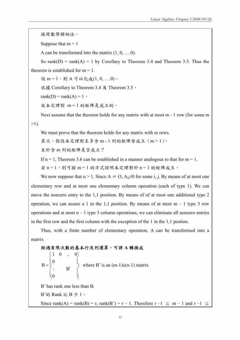
Linear Algebra- Chapter 3 20080926
12
採用數學歸納法
Suppose that m = 1
A can be transformed into the matrix (1 0 hellip0)
So rank(D) = rank(A) = 1 by Corollary to Theorem 34 and Theorem 35 Thus the
theorem is established for m = 1
設 m = 1則 A 可以化成(1 0 hellip0)
依據 Corollary to Theorem 34 及 Theorem 35
rank(D) = rank(A) = 1
故本定理對 m = 1 的矩陣是成立的
Next assume that the theorem holds for any matrix with at most m - 1 row (for some m
gt1)
We must prove that the theorem holds for any matrix with m rows
其次假設本定理對至多含 m - 1 列的矩陣皆成立(m gt 1)
至於含 m 列的矩陣是否成立
If n = 1 Theorem 36 can be established in a manner analogous to that for m = 1
若 n = 1則可按 m = 1 的方式證明本定理對於 n = 1 的矩陣成立
We now suppose that n gt 1 Since A ne O Aijne0 for some i j By means of at most one
elementary row and at most one elementary column operation (each of type 1) We can
move the nonzero entry to the 11 position By means of of at most one additional type 2
operation we can assure a 1 in the 11 position By means of at most m ndash 1 type 3 row
operations and at most n ndash 1 type 3 column operations we can eliminate all nonzero entries
in the first row and the first column with the exception of the 1 in the 11 postion
Thus with a finite number of elementary operation A can be transformed into a
matrix
經過有限次數的基本行及列運算可將 A 轉換成
⎪⎪⎭
⎪⎪⎬
⎫
⎪⎪⎩
⎪⎪⎨
⎧
=
0B
0001
B where Brsquo is an (m-1)times(n-1) matrix
Brsquo has rank one less than B
Brsquo的 Rank 比 B 少 1
Since rank(A) = rank(B) = r rank(Brsquo) = r ndash 1 Therefore r ndash1 ≦ m ndash 1 and r ndash1 ≦
Linear Algebra- Chapter 3 20080926
13
n ndash 1 by the induction hypothesis Hence r ≦ m and r ≦ n
由於 rank(A) = rank(B) = r故 rank(Brsquo) = r ndash 1
依數學歸納法 r ndash1 ≦ m ndash 1 且 r ndash1 ≦ n ndash 1
因此 r ≦ m 且 r ≦ n
Also by the induction hypothesis Brsquo can be transformed by a finite number of
elementary row and column operations into the (m-1)times(n-1) matrix Drsquo such that
同樣地依據數學歸納法Brsquo 可經過有限次數的基本行與列運算轉換成 (m-
1)times(n-1) 的矩陣 Drsquo使得
Dlsquo= ⎟⎟⎠
⎞⎜⎜⎝
⎛ minus
65
41r
OOOI
where O4 O5 and O6 are zero matrices
That is Drsquo consists of all zeros except for its first r-1 diagonal entries which are ones
Let
⎪⎪⎭
⎪⎪⎬
⎫
⎪⎪⎩
⎪⎪⎨
⎧
=
0D
0001
D
We see that the theorem now follows once we show that D can be obtained from B by
means of a finite number of elementary row and column operations
D 可由 B 經過有限次基本行及列運算而取得
Thus since A can be transformed into B and B can be transformed into D each by a
finite number of elementary operations A can be transformed into D by a finite number of
elementary operations
經過有限次基本行及列運算A B D
Finally since Drsquo contains ones as its first r ndash 1 diagonal entries D contains ones as its
first r diagonal entries and zeros elsewhere
最後Drsquo沿對角線前 r-1 個位置皆為 1故 D 沿對角線前 r 個位置皆為 1其餘
各處皆為 0
EXAMPLE 3 Consider the maxtrix
⎟⎟⎟⎟⎟
⎠
⎞
⎜⎜⎜⎜⎜
⎝
⎛
=
192362100280844422420
A
Linear Algebra- Chapter 3 20080926
14
By means of a succession of elementary row and column operations we can transform
A into a matrix D as in Theorem 36
透過一系列的基本行與列運算將 A 轉換成 D
D
00000001000001000001
192362100280844422420
A =
⎟⎟⎟⎟⎟
⎠
⎞
⎜⎜⎜⎜⎜
⎝
⎛
==
⎟⎟⎟⎟⎟
⎠
⎞
⎜⎜⎜⎜⎜
⎝
⎛
=
By the corollary to Theorem 34 rank(A) = rank(D) Clearly however rank(D) = 3 so rank(A) = 3
Corollary 1 Let A be an mtimesn matrix of rank r Then there exist invertible matrices B and C of sizes
mtimesm and ntimesn respectively such that D = BAC where D = ⎟⎟⎠
⎞⎜⎜⎝
⎛
32
1r
OOOI
is the mtimesn matrix
in which O1 O2 and O3 are zero matrices
令 A 為 mtimesn 的矩陣Rank 為 r存在可逆的 mtimesm 矩陣 B 與 ntimesn 矩陣 C使得
D = BAC其中D = ⎟⎟⎠
⎞⎜⎜⎝
⎛
32
1r
OOOI
為 mtimesn 的矩陣O1O2 及 O3 為零矩陣
【Proof】
By Theorem 36 A can be transformed by means of a finite number of elementary
row and column operations into the matrix D
We can appeal to Theorem 31 each time we perform an elementary operation Thus
there exist elementary mtimesm matrices E1 E2hellipEp and elementary ntimesn matrices G1
G2hellipGq such that D = EpEp-1hellipE2E1AG1G2hellipGq
By Theorem 32 each Ej and Gj is invertible Let B = EpEp-1hellipE2E1 and C =
G1G2hellipGq Then B and C are invertible and D = BAC
依據 Theorem 36A 可經過有限次的基本列與行運算化成 D
引用 Theorem 31每一次皆實施某一個基本列運算於是存在基本的 mtimesm 矩
陣 E1 E2hellip Ep 與 基 本 的 ntimesn 矩 陣 G1 G2hellip Gq 使 得 D = EpEp-
1hellipE2E1AG1G2hellipGq
依據 Theorem 32 每一個基本矩陣 Ej與 Gj 皆為可逆令 B = EpEp-1hellipE2E1 與 C =
G1G2hellipGq於是 B 與 C 皆為可逆且 D = EpEp-1hellipE2E1AG1G2hellipGq = BAC
Linear Algebra- Chapter 3 20080926
15
Theorem 31 令 AisinMmtimesn(F)並假設 B 是由 A 經實施某一基本列【或行】運算後所得
到的矩陣則存在一個 mtimesm 【或 ntimesn】基本矩陣 E使得 B = EA【或 B = AE】E
矩陣是由 Im 【或 In】 經實施與「由 A 得到 B」相同的基本列【或行】運算後所得
到的矩陣反之若 E 是一個 mtimesm【或 ntimesn】的基本矩陣則 EA【或 AE】是由 A
經過與「由 Im 【或 In】 得到 E」相同的基本列【或行】運算後所得到的矩陣
Theorem 32 基本矩陣為可逆矩陣且基本矩陣的反矩陣亦是同一型的基本矩陣
Theorem 36 令 A 為 Rank 等於 r 的 mtimesn 矩陣則 r m≦ 且 r n≦ 經過有限次數的基
本行與列運算讓 A 化成 D = ⎟⎟⎠
⎞⎜⎜⎝
⎛
32
1r
OOOI
其中Ir為對角元素為 1 的對角矩陣
Corollary 2 Let A be an mtimesn matrix Then
(a) rank(At) = rank(A)
矩陣轉置後的 RANK 不變
(b) The rank of any matrix equals the maximum number of its linearly independent
rows that is the rank of a matrix is the dimension of the subspace generated by
rows
任一矩陣的 Rank 等於最大線性獨立列向量的數目即矩陣的 Rank 等於由該
矩陣列向量所生成的子空間的維度
(c) The rows and columns of any matrix generate subspaces of the same dimension
numerically equal to the rank of the matrix
任一矩陣的列向量與行向量生成的子空間的維度相同維度等於該矩陣的
Rank
【Proof】
By Corollary 1 there exist invertible matrices B and C such that D = BAC where D
satisfies the stated conditions of the corollary Taking transposes we have
Dt = (BAC) t = CtAtBt
Since B and C are invertible so are Bt and Ct
Hence by Theorem 34 rank(At) = rank(CtAtBt) = rank(Dt)
Suppose that r = rank(A)
Then Dt is an ntimesm matrix with the form of the matrix D in Corollary 1 and hence
Linear Algebra- Chapter 3 20080926
16
rank(Dt) = r by Theorem 35
Thus
rank(At) = rank(Dt) = r = rank(A)
依據 Corollary 1存在可逆矩陣 B 與 C使得 D = BAC
取其轉置可得Dt = (BAC) t = CtAtBt
由於 B 與 C 為可逆故 Bt 與 Ct 亦為可逆
依據 Theorem 34得知 rank(At) = rank(CtAtBt) = rank(Dt)
設 r = rank(A)
則 Dt為一 ntimesm 的矩陣型式與 D 相同(參考 Corollary 1)
且依據 Theorem 35 得知 rank(Dt) = r
於是 rank(At) = rank(Dt) = r = rank(A)
Theorem 34 Let A be an mtimesn matrix If P and Q are invertible mtimesm and ntimesn matrices
respectively then 令 A 為 mtimesn 的矩陣若 P 與 Q 分別為可逆的 mtimesm 與 ntimesn 矩陣
則
(a) rank(AQ) = rank(A)
(b) rank(PA) = rank(A)
(c) rank(PAQ) = rank(A)
Theorem 35 The rank of any matrix equals the maximum number of its linearly
independent columns that is the rank of a matrix is the dimension of the subspace
generated by its column 任一矩陣的 Rank 等於其最大線性獨立行向量數目即矩陣
的 Rank 是由矩陣的行向量生成的子空間的維度【LA Fn Fm】
Corollary 3 Every invertible matrix is a product of elementary matrices
每一可逆矩陣均可為基本矩陣的乘積
【Proof】
If A is an invertible ntimesn matrix then rank(A) = n Hence the matrix D in Corollary 1
equals In and there exist invertible matrices B and C such that In = BAC
As in the proof of Corollary 1 note that B = EpEp-1hellipE2E1 and C = G1G2hellipGq where
the Eirsquos and Girsquos are elementary matrices Thus A = B-1InC-1 = B-1C-1 so that
A = E1-1E2
-1hellipEp-1Gq
-1Gq-1-1hellipG1
-1
Linear Algebra- Chapter 3 20080926
17
The inverses of elementary matrices are elementary matrices however and hence A is
the product of elementary matrices
若 A 為可逆的 ntimesn 矩陣則 rank(A) = n
因此 Corollary 1 中的矩陣 D 為 In且存在可逆的 B 與 C 矩陣使得 In = BAC
如同 Corollary 1 的證明一樣B = EpEp-1hellipE2E1 且 C = G1G2hellipGq其中Eirsquos 與
Girsquos 皆為基本矩陣
於是A = B-1InC-1 = B-1C-1即 A = E1-1E2
-1hellipEp-1Gq
-1Gq-1-1hellipG1
-1
基本矩陣的反矩陣亦為基本矩陣A 是基本矩陣的乘積
Theorem 37 Let T V W and U W Z be linear transformations on finite-dimensional vector
spaces V W and Z and let A and B be matrices such that the product AB is defined Then
令 VW 與 Z 為有限維度的向量空間T V W 與 U W Z 為線性轉換且
A 與 B 為滿足乘積 AB 定義的矩陣則
(a) rank(UT) ≦ rank(U)
(b) rank(UT) ≦ rank(T)
(c) rank(AB) ≦ rank(A)
(d) rank(AB) ≦ rank(B)
【Proof】
(a) Clearly R(T)subeW
Hence R(UT) = UT(V) = U(R(T)) sube U(W) = R(U)
Thus rank(UT) = dim(R(UT)) ≦ dim (R(U)) = rank(U)
(c) By (a) rank(AB) = rank(LAB) = rank (LALB) ≦ rank(LA) = rank(A)
(d) By (c) and Corollary 2 to Theorem 36
rank(AB) = rank((AB)t) = rank(B t A t) ≦ rank(B t) = rank (B) (b) Let α β and γ be ordered bases for V W and Z respectively and let Arsquo = γ
β]U[
and Brsquo = βα]T[ Then ArsquoBrsquo = γ
α]UT[ by Theorem 211
Hence by Theorem 33 and (d)
rank(UT) = rank(ArsquoBrsquo) ≦ rank(Brsquo) = rank (T)
Theorem 211 Let V W and Z be finite-dimensional vector space with ordered bases α β
and γ respectively Let T V W and U W Z be linear transformation Then
Linear Algebra- Chapter 3 20080926
18
βα
γβ
γα = [T][U][UT] 令 VW 與 Z 是有限維度的向量空間αβ 與 γ 分別為 VW 與
Z 的有序基底令 T V W (先 α β) 且 U W Z (後 β γ)則 βα
γβ
γα = [T][U][UT]
Theorem 33 Let T V W be a linear transformation between finite dimensional vector
spaces and let β and γ be ordered bases for V and W respective Then rank(T) = rank( γ
β[T] ) 令 T V W且 β 與 γ 分別為有限維度向量空間 V 與 W 的有序基底
則 rank(T) = rank( γβ[T] )
EXAMPLE 4
(a) Let ⎟⎟⎠
⎞⎜⎜⎝
⎛minus
=11111121
A (第一列與第二列是 LI) rank(A) = 2
(b) Let ⎟⎟⎟
⎠
⎞
⎜⎜⎜
⎝
⎛=
003011011131
A (第三列與第一二列是 LD)rank(A) = 2
(c) Let ⎟⎟⎟
⎠
⎞
⎜⎜⎜
⎝
⎛
minus=
011111121321
A (三列為 LI) rank(A) = 3
The inverse of a Matrix
We have remarked that an ntimesn matrix is invertible if and only if its rank is n Since we
know how to compute the rank of any matrix we can always test a matrix to determine
whether it is invertible We now provide a simple technique for computing the inverse of a
matrix that utilizes elementary row operations
已知 ntimesn 矩陣為可逆的『若且唯若』條件為該矩陣的 Rank 等於 n
DEFINITION 34 Augmented Matrix Let A and B be mtimesn and mtimesp matrices respectively By the augmented matrix )BA(
we mean that the mtimes(n+p) matrix )BA( that is the matrix whose first n columns are the
columns of A and whose last p columns are the columns of B 設 A 與 B 分別為 mtimesn 與 mtimesp 的矩陣則增廣矩陣(Augmented matrix) )BA(
Linear Algebra- Chapter 3 20080926
19
為一 mtimes(n+p)的矩陣 )BA( 該矩陣的前 n 行(Column)為 A 的所有的行後 p
行為 B 的所有行
Let A be an invertible ntimesn matrix and consider the ntimes2n augmented matrix C= )IA( n
C= )IA( n )AI()IAAA(CA 1
nn111 minusminusminusminus ==
By Corollary 3 to Theorem 36 A-1 is the product of elementary matrices say
A = EpEp-1hellipE2E1 (A-1 是多個基本矩陣的乘積)
Thus )AI()IAAA(CA 1
nn111 minusminusminusminus == )AI(CA)IA(EEE 1
n1
n11ppminusminus
minus ==
We have the following result If A is an invertible invertible ntimesn matrix then it is
possible to transform the matrix (AIn) into the matrix (InA-1) by means of a finite
number of elementary row operations
若 A 為一可逆的 ntimesn 矩陣則可經過有限次數的基本列運算將矩陣 (AIn) 化成
(InA-1)
Conversely suppose that A is invertible and that for some ntimesn matrix B the matrix
(AIn) can be transformed into the matrix (InB) by a finite number of elementary row
operations Let E1 E2hellip Ep be the elementary matrices associated with these elementary row
operations as in Theorem 31 then
反之假設 A 是可逆且矩陣(AIn)可經有限次數的基本列運算轉換成矩陣(InB)
並令 E1 E2hellip Ep 分別為 Theorem 31 所稱的基本矩陣則
)BI()IA(EEE nn11pp =minus
Let M = EpEp-1hellipE2E1 we have 令 M = EpEp-1hellipE2E1
)BI()IA(EEE nn11pp =minus )BI()IA(M)MMA( nn ==
Linear Algebra- Chapter 3 20080926
20
Hence MA = In and M = B It follows that M = A-1 So B = A-1
可由 MA = In 及 M = B 得知M 就是 A-1故 B 就是 A-1
Thus we have the follow resultsIf A is an invertible ntimesn matrix and the matrix
(AIn) is transformed in a matrix of the form (InB) by means of a finite number of
elementary row operations then B=A-1
若 A 為一可逆的 ntimesn 矩陣且矩陣 (AIn) 可經有限次數的基本列運算化成
(InB)則 B=A-1
If on the other hand A is an ntimesn matrix that is not invertible then rank(A) lt n Hence
any attempt to transform (AIn) into a matrix of the form (InB) by means of elementary row
operations must fail
反之若 A 是一不可逆的 ntimesn 矩陣則 rank(A) lt n因此任何想利用基本列運算
要將矩陣 (AIn) 化成 (InB)的努力必定失敗
Thus we have the follow results If A is an notinvertible ntimesn matrix then any attempt
to transform (AIn) into a matrix of the form (InB) produce a row whose first n entries
are zeros
若 A 是一不可逆的 ntimesn 矩陣任何想將矩陣 (AIn) 化成 (InB)的努力最後會
產生一前 n 個元素均為 0 的列
EXAMPLE 5
We determine whether the matrix ⎟⎟⎟
⎠
⎞
⎜⎜⎜
⎝
⎛=
133242420
A is invertible and if it is we
compute its inverse
A 是否為可逆矩陣
We attempt to use elementary row operations to transfer
Linear Algebra- Chapter 3 20080926
21
⎟⎟⎟
⎠
⎞
⎜⎜⎜
⎝
⎛=
100010001
133242420
)IA( into a matrix of the form (InB)
看看能否利用基本行與列運算將矩陣 (AIn) 化成 (InB)
Interchanging rows 1 and 2
⎟⎟⎟
⎠
⎞
⎜⎜⎜
⎝
⎛
100001010
133420242
Multiplying the first row by 12
⎟⎟⎟
⎠
⎞
⎜⎜⎜
⎝
⎛
10000100
133420121 2
1
Adding -3 times row 1 to row 3
⎟⎟⎟
⎠
⎞
⎜⎜⎜
⎝
⎛
minusminusminus 1000100
230420121
23
21
Multiplying row 2 by 12 to obtain 1 in the 22 position
⎟⎟⎟
⎠
⎞
⎜⎜⎜
⎝
⎛
minus
minus
minusminus 100000
230210121
23
21
21
Adding -2 times row 2 to row 1 and 3 times row 2 to row 3
⎟⎟⎟
⎠
⎞
⎜⎜⎜
⎝
⎛
minus
minusminus
10001
400210301
23
2321
21
Multiplying row 3 by 14
⎟⎟⎟
⎠
⎞
⎜⎜⎜
⎝
⎛
minus
minusminus
41
83
8321
21
0001
100210301
Adding appropriate multiply of row 3 to row 1 and 2 completes the process
⎟⎟⎟
⎠
⎞
⎜⎜⎜
⎝
⎛
minusminus
minus
41
83
83
21
43
41
43
85
81
100010001
目標達成
Thus A is invertible and ⎟⎟⎟
⎠
⎞
⎜⎜⎜
⎝
⎛
+minus+minus+minus+minus+
=minus
41
83
83
21
43
41
43
85
81
1A
Linear Algebra- Chapter 3 20080926
22
EXAMPLE 6
We determine whether the matrix ⎟⎟⎟
⎠
⎞
⎜⎜⎜
⎝
⎛minus=451112
121A is invertible and if it is we
compute its inverse
A 是否為可逆矩陣
We attempt to use elementary row operations to transfer
⎟⎟⎟
⎠
⎞
⎜⎜⎜
⎝
⎛minus=
100010001
451112
121)IA( into a matrix of the form (InB)
看看能否利用基本行與列運算將矩陣 (AIn) 化成 (InB)
Adding -2 times row 1 to row 2 and -1 times row 1 to row 3 then addig row 2 to row
3
⎟⎟⎟
⎠
⎞
⎜⎜⎜
⎝
⎛minus
100010001
451112
121
⎟⎟⎟
⎠
⎞
⎜⎜⎜
⎝
⎛
minusminusminusminus
101012001
330330
121
⎟⎟⎟
⎠
⎞
⎜⎜⎜
⎝
⎛
minusminusminusminus
113012001
000330
121
is a matrix with row whose first 3 entries are zeros Therefore A is not invertible
最後一列前 3 個元素均為 0
EXAMPLE 7 Let T P2(R) P2(R) be defined by T(f(x)) = f(x)+frsquo(x)+frdquo(x) where frsquo(x) and frdquo(x)
denote the first and second derivatives of f(x) We use Corollary 1 to Theorem 218 to test
T for invertibility and compute the inverse if T is invertible Taking β=1 x x2 to be the
standard ordered basis of P2(R) we have
令 T P2(R) P2(R) 為線性轉換且定義為 T(f(x)) = f(x)+frsquo(x)+frdquo(x)利用
Corollary 1 to Theorem 218 來測試 T 是否可逆並計算其逆轉換取 β=1 x x2為
P2(R)的標準有序基底
T(1) = 1 = 1bull1+0bullx+0bullx2
T(x) = 1+x = 1bull1+1bullx+0bullx2
Linear Algebra- Chapter 3 20080926
23
T(x2) = 2+2x+x2 = 2bull1+2bullx+1bullx2
⎟⎟⎟
⎠
⎞
⎜⎜⎜
⎝
⎛=β
100210211
[T] 稱為 T 相對有序基底 β的座標向量
依據 Corollary 1 to Theorem 218 T 可逆『若且唯若』 β[T] 可逆且
1-1 )[T](][T minusββ =
Using the method of Examples 5 and 6 we can show that β[T] is invertible with
inverse
⎟⎟⎟
⎠
⎞
⎜⎜⎜
⎝
⎛minus
minus=minus
β
100210
011)([T] 1
Thus T is is invertible and βminusminus
β = ][T)([T] 11 Hence by Theorem 214 we have
⎟⎟⎟
⎠
⎞
⎜⎜⎜
⎝
⎛minusminus
=⎟⎟⎟
⎠
⎞
⎜⎜⎜
⎝
⎛
⎟⎟⎟
⎠
⎞
⎜⎜⎜
⎝
⎛minus
minus=++ β
minus
2
21
10
2
1
02
2101
aa2aaa
aaa
100210
011)]xaxa(a[T
Therefore T-1(a0+a1x+a2x2) = (a0-a1)+(a1-2a2)x+a2x2 Corollary 1 to Theorem 218 Let V be finite-dimensional vector space with an ordered basis β and let T V V be linear Then T is invertible if and only if β[T] is invertible
Furthermore 1-1 )[T](][T minusββ = V 為有限維度的向量空間β 是 V 的有序基底令 T
V V 為線性轉換 T 為可逆的『若且唯若』條件為 β[T] 可逆再者
1-1 )[T](][T minusββ =
Theorem 214 Let V and W be finite-dimensional vector spaces having ordered bases β and γ respectively and let T V W be linear Then for each uisinV we have β
γβγ = [u][T][T(u)]
V 與 W 為有限維度的向量空間β 與 γ分別 V 與 W 的有序基底令 T V W 為線
性轉換則 V 中的 u 映至 W 的結果 T(u) 相對於有序基底 γ 的座標向量為
βγβγ = [u][T][T(u)]
Invertible and Inverse of MATRIX Let A be an n times n matrix If a matrix B can be found such that AB = BA = In then A is
Linear Algebra- Chapter 3 20080926
24
said to be invertible and B is called the inverse of A (denote B = A-1 and A-k=(A-1)k )
If such a matrix B does not exist then A has no inverse
EXAMPLE
⎥⎦
⎤⎢⎣
⎡=
4321
A and ⎥⎦
⎤⎢⎣
⎡minus
minus=
21
23
12B
221
23
221
23
I1001
432112
BA
I100112
4321
AB
=⎥⎦
⎤⎢⎣
⎡=⎥
⎦
⎤⎢⎣
⎡⎥⎦
⎤⎢⎣
⎡minus
minus=
=⎥⎦
⎤⎢⎣
⎡=⎥
⎦
⎤⎢⎣
⎡minus
minus⎥⎦
⎤⎢⎣
⎡=
Thus AB = BA = I2 proving that the matrix A has inverse B
Theorem The inverse of an invertible matrix is unique
Let B and C be inverse of A
Thus AB = BA = In and AC = CA = In
Multiply both sides of the equation AB = In by C
C(AB) = CIn (CA)B = C
InB = C B = C
Thus an invertible matrix has only one inverse
How to find AHow to find A--11
Based on the GaussBased on the Gauss--Jordan algorithmJordan algorithmLet A be an invertible matrix Then AALet A be an invertible matrix Then AA--11=I=Inn
Let the columns of Let the columns of AA--11 be be XX11 XX22 helliphellip XXnn and the columns of I and the columns of Inn be be CC11CC22helliphellipCCnn
Find AFind A--11 by finding by finding XX11 XX22 helliphellip XXnn Write the equation AAWrite the equation AA--11=I=Inn in the formin the form
[ ] [ ]n21nn211 CCCI XXXALet LL ==minus
[ ] [ ][ ] [ ]n21n21
n21n21
CCCAXAXXACCCXXXALL
LL
=rArr=
nn2211 CAXCAX CAX === LThus
How to find AHow to find A--11
Solving these systems by using Gauss-Jordan elimination on the large augmented matrix [AC1 C2hellipCn]
Thus when A-1 exits
[ ] [ ] [ ] 1n
1nn ABwhereBIAIIA minusminus ==asympasympL
If the reduced echelon form of [If the reduced echelon form of [AIAInn] is computed and ] is computed and the first part is not of the form Ithe first part is not of the form Inn then A has no inversethen A has no inverse
[ ][ ]n21n
n21
XXXI CCCAmatrix augmented
LL
L
asympasymp
Linear Algebra- Chapter 3 20080926
25
Example Example 1212
⎥⎥⎥
⎦
⎤
⎢⎢⎢
⎣
⎡
minusminusminusminusminus
=100531010532001211
]IA[ 3
⎥⎥⎦
⎤
⎢⎢⎣
⎡minusminusminus
minusminus
+minus+
asymp
101320012110001211
1RR1R3
2)(R2
⎥⎥⎦
⎤
⎢⎢⎣
⎡minus
minusminusminusasymp
101320012110001211
R2)1(
⎥⎥⎥
⎦
⎤
⎢⎢⎢
⎣
⎡
minusminusminusminusminus
=531532211
ADetermine the inverse of
Example Example 2222
⎥⎥⎦
⎤
⎢⎢⎣
⎡
minusminusminusminus
minus++asymp
123100012110013101
R2)2(R3R2R1
⎥⎥⎦
⎤
⎢⎢⎣
⎡
minusminusminus
minus++asymp
123100135010010001
R3)1(R2R3R1
123135110
A 1
⎥⎥⎥
⎦
⎤
⎢⎢⎢
⎣
⎡
minusminusminus=minus
⎥⎥⎦
⎤
⎢⎢⎣
⎡
minusminus
minus
+minus+asymp
135000011210012301
3R2R3R2)1(R1
ExampleExampleDetermine the inverse of
⎥⎥⎦
⎤
⎢⎢⎣
⎡
minus=
412721511
A
⎥⎥⎦
⎤
⎢⎢⎣
⎡
minus=
100412010721001511
][ 3IA
⎥⎥⎦
⎤
⎢⎢⎣
⎡
minusminusminusminus
minus+minus+asymp
102630011210001511
R1)2(R31)R1(R2
There is no need to proceed further There is no need to proceed further The reduced echelon form cannot have a one in the (3 3) locatioThe reduced echelon form cannot have a one in the (3 3) location n
The reduced echelon form cannot be of the form [IThe reduced echelon form cannot be of the form [Inn B] B] Thus Thus AAndashndash11 does not existdoes not exist
Properties of Matrix InverseProperties of Matrix Inverse
Let Let AA and and BB be invertible matrices andbe invertible matrices and cc a nonzero scalar a nonzero scalar ThenThen
AA =minusminus 11)( 111 1)( 2 minusminus = A
ccA
111)( 3 minusminusminus = ABAB
nn AA )()( 4 11 minusminus =tt AA )()( 5 11 minusminus =
Color Models Color Models 1212
A color model in the context of graphics is a method of A color model in the context of graphics is a method of implementing colorsimplementing colorsThe common used models include RGB model and YIQ modelThe common used models include RGB model and YIQ modelThe RGB model is used in computer monitors and the YIQ model The RGB model is used in computer monitors and the YIQ model is used in television screensis used in television screensAn RGB computer signal can be converted to a YIQ television An RGB computer signal can be converted to a YIQ television signal using the matrix transformationsignal using the matrix transformation
⎥⎥⎥
⎦
⎤
⎢⎢⎢
⎣
⎡
⎥⎥⎥
⎦
⎤
⎢⎢⎢
⎣
⎡
minusminusminus=
⎥⎥⎥
⎦
⎤
⎢⎢⎢
⎣
⎡
BGR
311523212321275596
114587299
QIY
YIQgtRGBYIQgtRGB
Color Models Color Models 2222
A signal is converted from a television screen to a computer monA signal is converted from a television screen to a computer monitor itor using inverse of the above matrixusing inverse of the above matrix
⎥⎥⎥
⎦
⎤
⎢⎢⎢
⎣
⎡
⎥⎥⎥
⎦
⎤
⎢⎢⎢
⎣
⎡
minusminusminus=
⎥⎥⎥
⎦
⎤
⎢⎢⎢
⎣
⎡rArr
⎥⎥⎥
⎦
⎤
⎢⎢⎢
⎣
⎡
⎥⎥⎥
⎦
⎤
⎢⎢⎢
⎣
⎡
minusminusminus=
⎥⎥⎥
⎦
⎤
⎢⎢⎢
⎣
⎡minus
QIY
0751108116472721
6209561
BGR
QIY
311523212321275596
114587299
BGR 1
CryptographyCryptography 密碼學密碼學 1212
Cryptography is the process of coding and decoding messagesCryptography is the process of coding and decoding messagesThe technique can be traced back to the ancient Greeks Today The technique can be traced back to the ancient Greeks Today governments use sophisticated methods of coding and decoding governments use sophisticated methods of coding and decoding messagesmessagesOne type of code that is extremely difficult to break makes use One type of code that is extremely difficult to break makes use of a of a large matrix to encode a message large matrix to encode a message The receiver of the message decodes it using the inverse of the The receiver of the message decodes it using the inverse of the matrixmatrixThe first matrix is called the encoding matrix and its inverse The first matrix is called the encoding matrix and its inverse is is called the decoding matrixcalled the decoding matrix
Cryptography Cryptography 密碼學密碼學 2222
A A-1Message
Encoding MatrixEncoding Matrix
Decoded MessageTransmission
Decoding MatrixDecoding Matrix
Linear Algebra- Chapter 3 20080926
26
Example Example 1212
Let the message be Let the message be BUY IBM STOCKBUY IBM STOCKAnd the encoding matrix beAnd the encoding matrix be
⎥⎥⎥
⎦
⎤
⎢⎢⎢
⎣
⎡ minusminusminus
434110433
B U Y B U Y -- I B M I B M -- S T O C KS T O C K2 21 25 27 9 2 13 27 19 20 15 3 112 21 25 27 9 2 13 27 19 20 15 3 11
⎥⎥⎥
⎦
⎤
⎢⎢⎢
⎣
⎡ minusminusminusminusminus=
⎥⎥⎥
⎦
⎤
⎢⎢⎢
⎣
⎡
⎥⎥⎥
⎦
⎤
⎢⎢⎢
⎣
⎡ minusminusminus
2331372091431715418461146
222117196116169
27319225271527921112013272
434110433
EncodingEncoding
Example Example 2222
Let the message be Let the message be BUY IBM STOCKBUY IBM STOCKAnd the decoding matrix beAnd the decoding matrix be
⎥⎥⎥
⎦
⎤
⎢⎢⎢
⎣
⎡
minusminus 334344101
B U Y B U Y -- I B M I B M -- S T O C KS T O C K2 21 25 27 9 2 13 27 19 20 15 3 112 21 25 27 9 2 13 27 19 20 15 3 11
⎥⎥⎥
⎦
⎤
⎢⎢⎢
⎣
⎡=
⎥⎥⎥
⎦
⎤
⎢⎢⎢
⎣
⎡ minusminusminusminusminus
⎥⎥⎥
⎦
⎤
⎢⎢⎢
⎣
⎡
minusminus 27319225271527921112013272
2331372091431715418461146
222117196116169
334344101
DecodingDecoding
3-3 Systems of Linear Equations ndash Theoretical Aspects
The system of equations
mnmn22m11m
2nn2222121
1nn1212111
bxaxaxa
bxaxaxabxaxaxa
=+++
=+++=+++
(S)
were aij and bi (1≦i≦m and 1≦j≦n) are scalars in a field F and x1 x2hellipxn are n
variables taking values in F is called a system of m linear equations in n unknows over the
field F
上式稱為佈於 Field F 含有 n 個未知數m 個線性方程式的系統或方程組(system
of m linear equations in n unknows)
The mtimesn matrix
⎟⎟⎟⎟⎟
⎠
⎞
⎜⎜⎜⎜⎜
⎝
⎛
=
mn2m1m
n22221
n11211
aaa
aaaaaa
A is called the coefficient matrix of the
system (S)(係數矩陣) If we let
⎟⎟⎟⎟⎟
⎠
⎞
⎜⎜⎜⎜⎜
⎝
⎛
=
n
2
1
x
xx
x and
⎟⎟⎟⎟⎟
⎠
⎞
⎜⎜⎜⎜⎜
⎝
⎛
=
m
2
1
b
bb
b Then the system (S) may
be rewritten as a single matrix equation Ax = b(單一矩陣方程式)
To exploit the results that we have developed we often consider a system of linear
equations as a single matrix equation
Linear Algebra- Chapter 3 20080926
27
A solution to the system (S) is an n-tuple n
n
2
1
F
s
ss
s isin
⎟⎟⎟⎟⎟
⎠
⎞
⎜⎜⎜⎜⎜
⎝
⎛
= such that As = b The set of
all solutions to the system (S) is called the solution set of the system(解集合) System (S)
is called consistent(相容) if its solution set is nonempty otherwise it is called
inconsistent(不相容)
方程組(S)的解為一 n 序組該序組可以使 As = b方程組的所有解所成的集合
稱為該方程組的解集合(Solution set)方程組的解集合非空集合者稱為「相容」解
集合空集合者稱為「不相容」
EXAMPLE 1
Consider 6x2xx1xx3x2
321
321
=+minus=++
that is ⎟⎟⎠
⎞⎜⎜⎝
⎛=
⎟⎟⎟
⎠
⎞
⎜⎜⎜
⎝
⎛
⎟⎟⎠
⎞⎜⎜⎝
⎛minus 6
1
xxx
211132
3
2
1
(以矩陣表示)
This system has many solutions such as ⎟⎟⎟
⎠
⎞
⎜⎜⎜
⎝
⎛minus=
726
s and ⎟⎟⎟
⎠
⎞
⎜⎜⎜
⎝
⎛
minusminus=
34
8s
Consider 1xx0xx
21
21
=+=+
that is ⎟⎟⎠
⎞⎜⎜⎝
⎛=⎟⎟
⎠
⎞⎜⎜⎝
⎛⎥⎦
⎤⎢⎣
⎡10
xx
1111
2
1
顯然地方程組無解
We begin our study of system of linear equations by examining the class of
homogeneous system of linear equations 先討論齊次方程組
DEFINITION 35 Homogeneous amp Nonhomogeneous
A system Ax=b of m linear equations in n unknowns is said to be homogeneous if b=0
Otherwise the system is said to be nonhomogeneous
方程組 Ax = bb = 0 稱為齊次方程組否則稱為非齊次方程組
Any homogeneous system has at least one solution namely the zero vector The next
result gives further information about the set of solutions to a homogeneous system
Linear Algebra- Chapter 3 20080926
28
齊次方程組至少有一個解那就是『零向量』
Theorem 38 Let Ax = 0 be a homogeneous system of m linear equations in n unknowns over a field
F Let K denote the set of all solutions to Ax = 0 Then K = N(LA) hence K is a subspace
of Fn of dimension n - rank(LA) = n- rank(A)
令 Ax = 0 代表一佈於 Field 含有 n 個未知數m 個線性方程式的方程組若令
K 代表該方程組的解集合(Solution set)則 K = N(LA)K 為 Fn 內的子空間且其維
度為 n ndash rank (LA) = n - rank(A)
【Proof】
Clearly K = sisinFn As = 0 = N(LA) The second part now follows from the
dimension theorem
Nullity(T)+rank(T) = dim(V)
Nullity (LA) = dim (Fn) ndashrank (LA ) = n ndash rank (A)
DEFINTION 27 Let V and W be vector space and let T V W be linear We define
the null space (or kernel) N(T) of T to be the set of all vectors x in V such that T(x) = 0
that is N(T) = xisinV T(x) = 0 V 與 W 為向量空間且 T V W 為線性轉換定義
線性轉換 T 的 Null space 為 V 內所有滿足 T(x) = 0 的向量 x 所形成的集合註記為
N(T)Null space 的元素 x 經線性轉換 T 轉換後所對應的「像」為 0意即 T(x) = 0
Null space 內的元素的「像」皆為 0
DEFINITION 217 Let A be an mtimesn matrix with entries from a field F We denote by LA
the mapping LA Fn Fm defined by LA(x) = Ax (the matrix product A and x) for each
column vector xisinFn We call LA a left-multiplication transformation 令 A 是 mtimesn
的矩陣所有元素均來自 FLA 為 Fn 映至 Fm的線性轉換並定義為 LA(x) = Ax其中
x 為行向量(Column vector)且 xisinFnLA被稱為左乘法轉換
Theorem 23 (Dimension Theorem) Let V and W be vector spaces and let T V W be
linear If V is finite-dimensional then Nullity(T) + rank(T) = dim(V) T 的核次數
(Nullity)與秩(Rank)的和等於定義域的維度 dim(V)
Corollary Let Ax = 0 be a homogeneous system of m linear equations in n unknowns over a field
Linear Algebra- Chapter 3 20080926
29
F If m lt n the system Ax = 0 has a nonzero solution
令 Ax = 0 代表一佈於 Field 含有 n 個未知數m 個線性方程式的方程組若 m
lt n則該方程組具有一非零解
【Proof】
Suppose that m lt n Then rank(A) = rank (LA)≦m Hence dim(K) = n - rank(LA) ≧
n ndash m gt 0 where K = N(LA) Since dim(K) gt 0 Kne 0 Thus there exists a nonzero
vector sisinK so s is a nonzero solution to Ax = 0
設 m lt n則 rank(A) = rank (LA) ≦ m依據 Theorem 38K = sisinFn As = 0
= N(LA) = dim(K) = n - rank(LA) ≧ n ndash m gt 0表示 dim(K) gt 0Kne 0故存在非
零向量 s使得 Ax = 0
EXAMPLE 2
Consider 0xxx
0xx2x
321
321
=minusminus=++
Let ⎟⎟⎠
⎞⎜⎜⎝
⎛minusminus
=111
121A be the coefficient matrix of this system It is clear that rank(A)
= 2 If K is the solution set of this system then dim(K) = 3-2 = 1 Thus any nonzero
solution constitutes a basis for K
若 K 是方程組的解所組成的集合(簡稱為解集合)依 Theorem 38 得知 dim(K)
= 3 - 2 = 1因此任一非零解將形成 K 的基底
For example since ⎟⎟⎟
⎠
⎞
⎜⎜⎜
⎝
⎛minus32
1 is a solution to the given system
⎪⎭
⎪⎬
⎫
⎪⎩
⎪⎨
⎧
⎟⎟⎟
⎠
⎞
⎜⎜⎜
⎝
⎛minus32
1 is a basis for
K Thus any vector in K is of the form ⎟⎟⎟
⎠
⎞
⎜⎜⎜
⎝
⎛minus=
⎟⎟⎟
⎠
⎞
⎜⎜⎜
⎝
⎛minus
t3t2
t
32
1t where tisinR
例如因⎟⎟⎟
⎠
⎞
⎜⎜⎜
⎝
⎛minus32
1是方程組的一個解故
⎪⎭
⎪⎬
⎫
⎪⎩
⎪⎨
⎧
⎟⎟⎟
⎠
⎞
⎜⎜⎜
⎝
⎛minus32
1 為 K 的基底K 內的任一向量均
具有如下形式
⎟⎟⎟
⎠
⎞
⎜⎜⎜
⎝
⎛minus=
⎟⎟⎟
⎠
⎞
⎜⎜⎜
⎝
⎛minus
t3t2
t
32
1t
Linear Algebra- Chapter 3 20080926
30
We now turn to the study of nonhomogeneous systems Our next result shows that the
solution set of a nonhomogeneous system Ax = b can be described in terms of the solution of
the homogeneous system Ax = 0 We refer to the equation Ax = 0 as the homogeneous system
corresponding to Ax = b
以下將進一步探討「非齊次方程組」非齊次方程組 Ax = b 的解集合可利用齊次方
程組 Ax = 0 的解來加以說明因此我們可將 Ax = 0 視為 Ax = b 的齊次方程組
Theorem 39 Let K be the solution set of a system of linear equations Ax = b and let KH be the
solution set of the corresponding homogeneous system Ax = 0 Then for any solution s to
Ax = b K =s + KH = s+k kisinKH
設 K 為線性方程組 Ax = b 的解集合且 KH為對應的齊次方程組的解集合則
對 Ax = b 的任一個解 s 而言K =s + KH = s+k kisinKH
【Proof】
Let s be any solution to Ax = b
We must show that K =s + KH
If wisinK then Aw = b Hence
A(w - s) = Aw ndash As = b ndash b = 0
So w - sisinKH
Thus there exists kisinKH such that w - s = k
It follows that w = s + k isin s +KH and therefore Ksube s +KH
Conversely suppose that wisins +KH then w = s + k for some kisinKH
But then Aw = A(s + k) = As + Ak = b + 0 = b so wisinK
Therefore s +KHsubeK and thus K=s +KH
令 s 為 Ax = b 的任一個解我們必須證明「K =s + KH」
若 wisinK則 Aw = b(即 w 為 Ax = b 的解)
於是 A(w - s) = Aw ndash As = b ndash b = 0
所以 w - sisinKH(即 w-s 為 Ax = 0 的解)
w - s 既然是 KH的元素表示有一元素 kisinKH使得 w - s = kw = s + k
w = s + kisins +KH
Linear Algebra- Chapter 3 20080926
31
因此 Ksube s +KH
反之假設 wisins +KH則 KH中存在一元素 k(kisinKH)使得 w = s + k
因 Aw = A(s + k) = As + Ak = b + 0 = b
故 wisinK 是 Ax = b 的解
因此s +KHsubeK
總結K=s +KH
EXAMPLE 3
Consider 4xxx7xx2x
321
321
minus=minusminus=++
The corresponding homogeneous system is the system in Example 2 It is easily
verified that ⎟⎟⎟
⎠
⎞
⎜⎜⎜
⎝
⎛=
411
s is a solution to the preceeding nonhomogeneous system So the
solution set of the system is ⎪⎭
⎪⎬
⎫
⎪⎩
⎪⎨
⎧isin
⎟⎟⎟
⎠
⎞
⎜⎜⎜
⎝
⎛minus+
⎟⎟⎟
⎠
⎞
⎜⎜⎜
⎝
⎛= Rt
32
1t
411
K by Theorem 39
⎟⎟⎟
⎠
⎞
⎜⎜⎜
⎝
⎛=
411
s 是非齊次方程組 Ax = b 的解
⎟⎟⎟
⎠
⎞
⎜⎜⎜
⎝
⎛minus32
1是齊次方程組的解
依據 Theorem 39 得知線性方程組 Ax = b 的解集合⎪⎭
⎪⎬
⎫
⎪⎩
⎪⎨
⎧isin
⎟⎟⎟
⎠
⎞
⎜⎜⎜
⎝
⎛minus+
⎟⎟⎟
⎠
⎞
⎜⎜⎜
⎝
⎛= Rt
32
1t
411
K
The following theorem will provide us with a means of computing solutions to certain
system of linear equations
Theorem 310~311 提供計算線性方程組的解的方法
Theorem 310 Let Ax = b be a system of n linear equations in n unknowns If A is invertible then the
Linear Algebra- Chapter 3 20080926
32
system has exactly one solution namely A-1b Conversely if the system has exactly one
solution then A is invertible
令 Ax = b 為含 n 個未知數n 個線性方程式的方程組若 A 為可逆則方程組
恰有一個解解為 A-1b反之若該方程組恰有一個解則 A 為可逆
【Proof】
Suppose that A is invertible
Substituting A-1b into system we have A(A-1b)=( AA-1)b = b
Thus A-1b is a solution
If s is an arbitrary solution then As = b
Multiplying both sides by A-1 gives s= A-1b
Thus the system has one and only one solution namely A-1b
假設 A 為可逆將 A-1b 代入方程組可得 A(A-1b)=( AA-1)b = b
故 A-1b 確為方程組的解
若 s 為方程組的任意解則 As = b
兩邊乘上 A-1可得 s= A-1b
因此方程組僅有唯一的解 A-1b
Conversely suppose that the system has exactly one solution s
Let KH denot the solution set for the corresponding homogeneous system Ax = 0
By Theorem 39 s = s + KH But it is so only if KH = 0 Thus N(LA) = 0 and
hence A is invertible
反之假設方程組恰有一個解 s
令 KH為相對應齊次方程組 Ax = 0 的解集合
依據 Theorem 39要能s = s + KH唯有 KH = 0
KH = 0即表示 N(LA) = 0故 A 為可逆
EXAMPLE 4 Consider the following system of three linear equations in three unknowns
1xx3x33x2x4x2
2x4x2
321
321
32
=++=++
=+
In Example 5 of Section 32 we compute the inverse of the coefficient matrix A of
this system Thus the system has exactly one solution namely
Linear Algebra- Chapter 3 20080926
33
⎟⎟⎟
⎠
⎞
⎜⎜⎜
⎝
⎛=
133242420
A⎟⎟⎟
⎠
⎞
⎜⎜⎜
⎝
⎛
+minus+minus+minus+minus+
=minus
41
83
83
21
43
41
43
85
81
1A
⎟⎟⎟
⎠
⎞
⎜⎜⎜
⎝
⎛
minus+minus
=⎟⎟⎟
⎠
⎞
⎜⎜⎜
⎝
⎛
⎟⎟⎟
⎠
⎞
⎜⎜⎜
⎝
⎛
+minus+minus+minus+minus+
==⎟⎟⎟
⎠
⎞
⎜⎜⎜
⎝
⎛minus
814587
41
83
83
21
43
41
43
85
81
1
3
2
1
132
bAxxx
Theorem 311 Let Ax = b be a system of linear equations Then the system is consistent (相容)if
and only if rank(A) = rank (A∣b) Matrix (A b) is called the augmented matrix o∣ f the
system Ax = b
令 Ax = b 為線性方程式方程組則此方程組至少有一個解的『若且唯若』條件
為 rank(A) = rank (A∣b) 矩陣(A∣b)稱為方程組 Ax = b 的增廣矩陣
【Proof】
To say that Ax = b has a solution is equivalent to saying that bisinR(LA)
In the proof of Theorem 35 we saw that R(LA ) = span(a1 a2 an) the span of the
column of A
Thus Ax = b has a solution if and only if bisinspan(a1 a2 an)
But bisinspan(a1 a2 an) if and only if span(a1 a2 an) = span(a1 a2 an b)
This last statement is equivalent to
dim (span(a1a2an)) = dim (span(a1a2an b))
So by Theorem 35 the preceeding equation reduces to rank(A) = rank (A∣b)
Ax = b 有一解相當於 bisinR(LA)即 b 屬於線性轉換 LA的 Range
在 Theorem 35 的證明中提到 R(LA ) = span(a1a2an)aj 為 A 的第 j 個行
(Column)即線性轉換 LA 的 Range 係由矩陣 A 的行(Column)所生成
因此 Ax = b 要有一個解的『若且唯若』條件為 bisinspan(a1 a2 an)
至於 bisinspan(a1 a2 an)之條件
bisinspan(a1a2an) 的『若且唯若』條件為 span(a1a2an) = span(a1a2an
b)
其條件相當於
Linear Algebra- Chapter 3 20080926
34
dim (span(a1a2an)) = dim (span(a1a2an b))
依據 Theorem 35該條件可簡化為 rank(A) = rank (A∣b)
Theorem 35 The rank of any matrix equals the maximum number of its linearly
independent columns that is the rank of a matrix is the dimension of the subspace
generated by its column任一矩陣的 Rank 等於其最大線性獨立行向量數目即矩陣的
Rank 是由矩陣的行向量生成的子空間的維度【LA Fn Fm】
EXAMPLE 5 Recall the system of equations
1xx0xx
21
21
=+=+
Since ⎟⎟⎠
⎞⎜⎜⎝
⎛=
1111
A and ⎟⎟⎠
⎞⎜⎜⎝
⎛=
111011
)bA(
rank(A) = 1 and rank (A b) = 2∣
Because the two ranks are unequal the system has no solutions
矩陣 A 與增廣矩陣(A∣b) 的 Rank 不同故方程組沒有解
EXAMPLE 6 We can use Theorem 311 to determine whether (3 3 2) is in the range of the linear
transformation T R3 R3 defined by T(a1 a2 a3) = (a1+a2+a3 a1-a2+a3 a1+a3)
利用 Theorem 311 來判斷 (3 3 2)是否在線性轉換 T 的 Range 中其中T R3
R3 定義為 T(a1 a2 a3) = (a1+a2+a3 a1-a2+a3 a1+a3)
Now (3 3 2)isinR(T) if and only if there exists a vector s = x1 x2 x3 in R3 such that
T(s)=(3 3 2) Such a vector s must be a solution to the system
2xx3xxx3xxx
31
321
321
=+=+minus=++
Since the ranks of the coefficient matrix and the augmented matrix of this system
are 2 and 3 respectively it follows that this system has no solutions Hence (3 3 2) notin
R(T)
(3 3 2)isinR(T) 的『若且唯若』的條件為存在一向量 s = x1 x2 x3isinR3 使得
T(s)=(3 3 2)
Linear Algebra- Chapter 3 20080926
35
向量 s 必須是 2xx3xxx3xxx
31
321
321
=+=+minus=++
的解
因係數矩陣⎟⎟⎟
⎠
⎞
⎜⎜⎜
⎝
⎛minus
101111111
的 Rank 為 2增廣矩陣⎟⎟⎟
⎠
⎞
⎜⎜⎜
⎝
⎛minus
233
101111111
的 Rank 為 3兩
者不相等故方程組無解(3 3 2) notin R(T)
Theorem 311 Let Ax = b be a system of linear equations Then the system is consistent
(相容)if and only if rank(A) = rank (A∣b) Matrix (A b) is called the ∣ augmented
matrix of the system Ax = b 令 Ax = b 為線性方程式方程組則此方程組至少有一個
解的『若且唯若』條件為 rank(A) = rank (A∣b) 矩陣(A∣b)稱為方程組 Ax = b 的
增廣矩陣
Application
In 1973 Wassily Leontief won the Nobel prize in economics for his work in developing
a mathematical model that can be used to describe various economic phenomena
1973 年Wassily Leontief 因研究一數學模式來描述各種經濟現象而獲頒諾貝爾經
濟獎
CLOSED MODEL
We begin by considering a simple society composed of three peoples (industries) ndash a
farmer who gows all the food a tailor who makes all the clothing and a carpenter who builds
all the housing We assume that each person sells to and buy from a central pool and that
everything produced is consumed Since no commodities either enter or leave the system this
case is referred to as the CLOSE MODEL
考慮一個單純社會的三種人生產食物的農夫製衣的裁縫師與蓋住屋的木匠
並假設採取集中聯營買賣且每一件產品皆付諸消費由於過程中沒有任何成品進入
或脫離這個系統所以稱為「封閉模式」
Each of these three individual consumes all three of the commodities produced in the
Linear Algebra- Chapter 3 20080926
36
society Suppose that the proportion of each of the commodities consumed by each person is
given in the following table
社會中每一位皆消費所生產的三種成品且每一種產品也都被三位所消費其消
費比例如下
食物 Food 衣物 Clothing 住屋 Housing
農夫 Farmer 040 020 020
裁縫師 Tailor 010 070 020
木匠 Carpenter 050 010 060
Let p1 p2 and p3 denote the incomes of the farmer tailor and carpenter respectively To
ensure that this society survives we require that the consumption of each individual equals
his or her income
令 p1p2 與 p3 分別表示農夫裁縫師與木匠的收入並為確保這個封閉社會可以
存活假設每一位的收入等於消費
Note that the farmer consumes 20 of the clothing Because the total cost of all clothing
is p2 the tailorrsquos income the amount spent by the farmer on clothing is 020 p2 Moreover the
amount spent by the farmer on food clothing and housing must equal the farmerrsquos income
and so we obtain the equation 040 p1 + 020 p2 + 030 p3 = p1
對農夫而言農夫的衣物消費佔 20然因所有衣物的消費總額 p2 等於裁縫師的
收入所以農夫在衣物上的消費為 020 p2且農夫在食物衣物與住屋的總消費要等
於農夫的收入 p1所以農夫的收入與消費關係式
040 p1 + 020 p2 + 020 p3 = p1
Similary equations describing the expenditures of the tailor and carpenter produce the
following system of linear equations
同理分別對裁縫師與木匠進行討論可獲得下列方程組
Linear Algebra- Chapter 3 20080926
37
040 p1 + 020 p2 + 020 p3 = p1
010 p1 + 070 p2 + 020 p3 = p2
050 p1 + 010 p2 + 060 p3 = p3
This system can be written as Ap = p
其中⎟⎟⎟
⎠
⎞
⎜⎜⎜
⎝
⎛=
3
2
1
ppp
p 且⎟⎟⎟
⎠
⎞
⎜⎜⎜
⎝
⎛=
600100500200700100200200400
A 稱為輸入-輸出(或消費)矩陣
(Input-output (or consumption) matrix)
Ap = p 稱為均衡條件(Equilibrium condition)
能否利用不等式 p ≦ p 來替代等式
At first it may seem reasonable to replace the equilibrium condition by the inequality
Ap ≦ p that is the requirement that consumption not exceed production But in fact Ap ≦ p implies that Ap = p in the closed model
For otherwise there exists a k for which
sumgt
jjkjk pAp
Hence since the columns of A sum to 1
sumsumsumsum ==gt
jj
i jjij
ii ppAp which is a contradiction (出現矛盾)
答案是在封閉系統中Ap ≦ p Ap = p
One solution to the homogeneous system (I ndash A) x = 0 which is equivalent to the
equilibrium condition is ⎟⎟⎟
⎠
⎞
⎜⎜⎜
⎝
⎛=
400350250
p
Linear Algebra- Chapter 3 20080926
38
齊次方程組(I ndash A) x = 0 或均衡條件的一個解為 ⎟⎟⎟
⎠
⎞
⎜⎜⎜
⎝
⎛=
400350250
p
We may interpret this to mean that the society survives if the farmer taior and carpenter
have incomes in the proportions 253540
⎟⎟⎟
⎠
⎞
⎜⎜⎜
⎝
⎛=
400350250
p 可以解釋為若農夫裁縫師與木匠收入比例為 253540則社會將
能生存下去
Theorem 312
Let A be an ntimesn input-output matrix having the form ⎟⎟⎠
⎞⎜⎜⎝
⎛=
EDCB
A where D is a 1times(n-
1) positive vector and C is an (n-1)times1 positive vector Then (I-A)x = 0 has a one-
dimensional solution set that is generated by a nonnegative vector
設 A 為 ntimesn 輸入-輸出矩陣 ⎟⎟⎠
⎞⎜⎜⎝
⎛=
EDCB
A 其中D 為 1times(n-1)正向量C 為
(n-1)times1 正向量則(I-A)x = 0 具有一維解集合且該解集合係由一非負向量所生成
Any input-output matrix with all positive entries satisfies the hypothesis of this theorem
任何輸入-輸出矩陣滿足 Theorem 312 的基本假設條件例如
⎟⎟⎟
⎠
⎞
⎜⎜⎜
⎝
⎛=
02502503502500650500750
A
OPEN MODEL
In the OPEN MODEL we assume that there is an outside demand for each of the
commodities produced Returning to our simple society let x1 x2 and x3 be the monetary
values of food clothing and housing produced with respective outside demands d1 d2 and d3
Let A be the 3times3 matrix such that Aij represents the amount of commodity i required to
Linear Algebra- Chapter 3 20080926
39
produce one monetary unit of commodity j Then the value of the surplus of food in the
society is x1 ndash (A11x1+A12x2+A13x3) that is the value of food produced minus the value of
food consumed while producing the three commodities The assumption that everything
produced is consumed gives us a similar equilibrium condition for the open model namely
that the surplus of each of the three commodities must equal the corresponding outside
demands Hence i
3
1jjiji dxAx =minussum
=
for j=1 2 3
在「開放模式」中我們假設每一產品皆有外來的需求在前述的單純社會裡
令 x1x2 與 x3 分別代表食物衣物與住屋的貨幣價值d1d2 與 d3 為食物衣物與住
屋的外來需求價值令 A 為 3times3 矩陣Aij 表示生產『一個貨幣單位』的產品 j 所需要
的產品 i 的價值於是此社會中食物的盈餘價值為 x1 ndash (A11x1+A12x2+A13x3)即食物的
價值減去生產食物衣物與住屋所需消耗的食物的價值意即生產出來的食物價值扣
掉用去生產食物衣物與住屋所消耗掉的價值)(A11A12A13 為生產一個貨幣單位
的食物 1衣物 2 與住屋 3 所需消耗的食物 1 數量A12x2 表示生產貨幣價值為 x2的衣物
所需要的食物價值)對每一種產品而言其盈餘價值等於外來的需求價值於是
i
3
1jjiji dxAx =minussum
=
for j=123
Suppose that 30 cents worth of food 10 cents worth of clothing and 30 cents worth of
housing are required for the production of $1 worth of food Similar suppose that 20 cents
worth of food 40 cents worth of clothing and 20 cents worth of housing are required for the
production of $1 worth of clothing Finally suppose that 30 cents worth of food 10 cents
worth of clothing and 30 cents worth of housing are required for the production of $1 worth
of housing Then the input-output matrix is
⎟⎟⎟
⎠
⎞
⎜⎜⎜
⎝
⎛=
300200300100400100300200300
A
假設生產價值 1 元的食物需要價值 30 分的食物(A11 = 03)價值 10 分的衣物
(A21 = 01)及價值 30 分的住屋(A31 = 03)生產價值 1 元的衣物需要價值 20 分的
食物(A12 = 02)價值 40 分的衣物(A22 = 04)及價值 20 分的住屋(A32 = 02)生
Linear Algebra- Chapter 3 20080926
40
產價值 1 元的住屋需要價值 30 分的食物(A13 = 03)價值 10 分的衣物(A23 = 01)
及價值 30 分的住屋(A33 = 03)於是輸入輸出矩陣 A 為
⎟⎟⎟
⎠
⎞
⎜⎜⎜
⎝
⎛=
300200300100400100300200300
A
若食物的外來需求值為 300 億元衣物為 200 億元住屋值為 1 百億元則
⎟⎟⎟
⎠
⎞
⎜⎜⎜
⎝
⎛=
⎟⎟⎟
⎠
⎞
⎜⎜⎜
⎝
⎛
⎟⎟⎟
⎠
⎞
⎜⎜⎜
⎝
⎛
minusminusminusminusminusminus
=minus=
minus
minus
700600900
100200300
700200300100600100300200300
d)AI(x
1
1
⎟⎟⎟
⎠
⎞
⎜⎜⎜
⎝
⎛=
700600900
x 表示要滿足外來需求必須生產的食物價值為 900 億元衣物價值為
600 億元住屋價值為 700 億元
Theorem
Let AX = Y be a system of n linear equations in n variables If Andash1 exists the
solution is unique and is given by X = Andash1Y
【Proof】
Substitute X = Andash1Y into the matrix equation
AX = A(Andash1Y) = (AAndash1)Y = InY = Y
The solution is unique
Let X1 be any solution thus AX1 = Y Multiplying both sides of this equation by Andash1
gives
Andash1AX1= Andash1Y InX1 = Andash1Y X1 = Andash1Y
Linear Algebra- Chapter 3 20080926
41
Example Example 1212
2x5x3x3x5x3x21x2x x
321
321
321
minus=++minus=minusminus=minusminus
⎥⎥⎥
⎦
⎤
⎢⎢⎢
⎣
⎡
minus=
⎥⎥⎥
⎦
⎤
⎢⎢⎢
⎣
⎡
⎥⎥⎥
⎦
⎤
⎢⎢⎢
⎣
⎡
minusminusminusminusminus
231
xxx
531532211
3
2
1
Solve the system of equations
This system can be written in the following matrix form
⎥⎥⎥
⎦
⎤
⎢⎢⎢
⎣
⎡
minus⎥⎥⎥
⎦
⎤
⎢⎢⎢
⎣
⎡
minusminusminusminusminus
=
⎥⎥⎥
⎦
⎤
⎢⎢⎢
⎣
⎡minus
231
531532211
xxx 1
3
2
1
If the matrix of coefficients is invertible the unique solutionIf the matrix of coefficients is invertible the unique solution isis
Example Example 2222
1 2 1 issolution unique The 321 =minus== xxx
⎥⎥⎥
⎦
⎤
⎢⎢⎢
⎣
⎡minus=
⎥⎥⎥
⎦
⎤
⎢⎢⎢
⎣
⎡
minus⎥⎥⎥
⎦
⎤
⎢⎢⎢
⎣
⎡
minusminusminus=
⎥⎥⎥
⎦
⎤
⎢⎢⎢
⎣
⎡
121
231
123135110
xxx
3
2
1
⎥⎥⎥
⎦
⎤
⎢⎢⎢
⎣
⎡
minusminusminus=
⎥⎥⎥
⎦
⎤
⎢⎢⎢
⎣
⎡
minusminusminusminusminus
=
minus
minus
123135110
531532211
A
1
1
The The LeontiefLeontief IO Model in IO Model in Economics Economics 1515
The Leontief input-output model is used to analyze the interdependence of economics Wassily Leontief received a Nobel Prize in 1973 for his work in thie fieldThe practical applications of this model have proliferated until it has now become a standard tool for investigating economic structures ranging from cities and corporation to states and countriesConsider an economics situation that involves ninterdependent industries The output of any one industry is needed as input by other industries and even possibly by the industry itself
The The LeontiefLeontief IO Model in IO Model in Economics Economics 2525
How a mathematical model involving a system of linear equations can be constructed to analyze such a situationAssume that each industry produces one commodity Let aij denote the amount of input of a certain commodity i to produce unit output of commodity j In our model let the amounts of input and output be measured in dollars Thus for example a34 = 045 means that 45 centsrsquo worth of commodity 3 is required to produce one dollarrsquos worth of commodity 4
The The LeontiefLeontief IO Model in IO Model in Economics Economics 3535
aij = amount of commodity i in one dollar of commodity jaij =生產一元價值的j產品需要耗用的i產品價值
The elements aij called input coefficients define a matrix A called the input-output matrix which describes the interdependence of the industriesExtending the model to include an open sector (all non-producing sectors) The product of industries may go not only into other producing industries but also into other non-producing sectors of the economy such as consumers and governments
The The LeontiefLeontief IO Model in IO Model in Economics Economics 4545
di = demand of the open sectors from industry ixi=total output of industry I necessary to meet demands of all n industries and the open sector
sectoropen of demand
nindustry of demand
2industry of demand
22
1industry of demand
11
industry ofoutput total
ininii
i
i dxaxaxax ++sdotsdotsdot++=
output ofportion sectoropen
output ofportion tryinterindusoutput total
DAXX +=Demand matrixDemand matrix
Output matrixOutput matrix
The The LeontiefLeontief IO Model in IO Model in Economics Economics 5555
Applying the model to the economy of a country X Applying the model to the economy of a country X represents the total output of each of the producing sectors represents the total output of each of the producing sectors of the economy and AX describes the contributions made of the economy and AX describes the contributions made by the various sectors to fulfilling the intersectional input by the various sectors to fulfilling the intersectional input requirements of the economyrequirements of the economyD is equal to (XD is equal to (X--AX) the difference between total output AX) the difference between total output X and industry transaction AXX and industry transaction AXD is thus the gross national product of the economyD is thus the gross national product of the economy
Example Example 1414
Consider an economy consisting of three industries having Consider an economy consisting of three industries having the following inputthe following input--output matrix output matrix AA Determine the output Determine the output levels required of the industries to meet the demands of levels required of the industries to meet the demands of the other industries and of the open sector in each casethe other industries and of the open sector in each case
in turn 321812
and 896
1612
9
5100
021
21
103
51
51
⎥⎥⎦
⎤
⎢⎢⎣
⎡
⎥⎥⎦
⎤
⎢⎢⎣
⎡
⎥⎥⎦
⎤
⎢⎢⎣
⎡=
⎥⎥⎥
⎦
⎤
⎢⎢⎢
⎣
⎡
= DA
The unit of The unit of DD are millions of dollarsare millions of dollars
Linear Algebra- Chapter 3 20080926
42
Example Example 2424
We wish to compute the output levels X that correspond to We wish to compute the output levels X that correspond to the various open sector demands D X is given by the the various open sector demands D X is given by the equation X = AX + D Rewritten as followsequation X = AX + D Rewritten as follows
X ndash AX = D rArr (I ndash A)X = D rArr X = (I ndash A) ndash1 D
⎥⎥⎥
⎦
⎤
⎢⎢⎢
⎣
⎡
=⎥⎥⎥
⎦
⎤
⎢⎢⎢
⎣
⎡
minus⎥⎥⎦
⎤
⎢⎢⎣
⎡=minus minus
minusminus
5400
021
21
103
51
54
5100
021
21
103
51
31
100010001
get We AI
⎥⎥⎥
⎦
⎤
⎢⎢⎢
⎣
⎡
=minus minus
4500
038
35
85
32
35
1)( AI
output ofingcorrespond valuesvarious
4500
038
35
85
32
35
)(
401020883957522133
32816189121269
)(
1
1
DAI
DAIX
minus
minus
minusuarruarruarruarruarruarruarr
⎥⎥⎦
⎤
⎢⎢⎣
⎡=
⎥⎥⎦
⎤
⎢⎢⎣
⎡
⎥⎥⎥
⎦
⎤
⎢⎢⎢
⎣
⎡
=minus=
Example Example 3434
By using Gauss-Jordan elimination
dollars of milliond are units The
40
15674
and 106629
209946
are 321812
and 896
1612
9
⎥⎥⎥
⎦
⎤
⎢⎢⎢
⎣
⎡
⎥⎥⎥
⎦
⎤
⎢⎢⎢
⎣
⎡
⎥⎥⎥
⎦
⎤
⎢⎢⎢
⎣
⎡
⎥⎥⎥
⎦
⎤
⎢⎢⎢
⎣
⎡
⎥⎥⎥
⎦
⎤
⎢⎢⎢
⎣
⎡
⎥⎥⎥
⎦
⎤
⎢⎢⎢
⎣
⎡
Example Example 4444
The output levels necessary to meet the demandsThe output levels necessary to meet the demands
IAAAIAI m =++++minus ))(( 2 L
mAAAIAI ++++=minus minus L21)(
Computing (IComputing (I--A) A) --11
1m
m2m2
m2
AI)AAAI(A)AAAI(I
)AAAI)(AI(
+minus=++++minus++++=
++++minusLL
L
NOTE 0A 1m rarr+
Population Movement Population Movement 1313
In 2000 58 million of people live in cities and 142 million of In 2000 58 million of people live in cities and 142 million of people people live in the surrounding suburbs Represent this information by tlive in the surrounding suburbs Represent this information by the he matrix matrix
The probability of a person staying in the city was 096 Thus tThe probability of a person staying in the city was 096 Thus the he probability of moving to the suburbs was 004 probability of moving to the suburbs was 004 The probability of a person moving to the city was 001 the The probability of a person moving to the city was 001 the probability of remaining in suburbia was 099probability of remaining in suburbia was 099
suburbcity
990040010960
suburbcity (to))from(
⎥⎦
⎤⎢⎣
⎡=P
⎥⎦
⎤⎢⎣
⎡=
14258
X0
City population in 2001 = people who remained from 2000 + peopleCity population in 2001 = people who remained from 2000 + peoplewho moved in from the suburbs = ( 096 who moved in from the suburbs = ( 096 timestimes 58 ) + (001 58 ) + (001 timestimes 142 ) = 142 ) = 571 million571 millionSuburban population in 2001 = people who moved in from the city Suburban population in 2001 = people who moved in from the city + people who stayed from 2000 = ( 004 + people who stayed from 2000 = ( 004 timestimes 58 ) + (099 58 ) + (099 timestimes 142 ) = 142 ) = 1429 million1429 millionCan arrive at these numbers using matrix multiplicationCan arrive at these numbers using matrix multiplication
⎥⎦
⎤⎢⎣
⎡=⎥
⎦
⎤⎢⎣
⎡⎥⎦
⎤⎢⎣
⎡==
9142157
14258
990040010960
PXX 01
Population Movement Population Movement 2323
Population Movement Population Movement 3333
Assume that the population flow represented by the matrix P is unchanged over the years The population distribution X2 after 2 years is given by X2 = P X1 = P2 X0 In general
Pn is called the n-step transition matrix The (ij)th element of Pngives the probability of going from state j to state i in n stepsFor example
in
ni XPX =+
suburbcity
960150040850
P
suburbcity (to))from(
4
⎥⎦
⎤⎢⎣
⎡=
The probability of living in the city in The probability of living in the city in 2000 and being in the suburbs 4 years 2000 and being in the suburbs 4 years later is 015later is 015
Markov ChainsMarkov Chains
The probabilities in the above model depend only on the The probabilities in the above model depend only on the current state of a person whether the person is living in the current state of a person whether the person is living in the city or in suburbiacity or in suburbiaThis type of model in which the probability of going from This type of model in which the probability of going from one state to another depends only on the current state one state to another depends only on the current state rather than on a more complete historical description is rather than on a more complete historical description is called a called a Markov chainMarkov chainMarkov chains are useful tools for scientists in many Markov chains are useful tools for scientists in many fields such as geneticsfields such as genetics
Linear Algebra- Chapter 3 20080926
43
GeneticsGenetics 1414
Genetics is the branch of biology that deals with Genetics is the branch of biology that deals with heredity heredity (遺傳)(遺傳) It is the study of units called It is the study of units called genes which determine the characteristics living genes which determine the characteristics living things inherit from their parents The inheritance things inherit from their parents The inheritance (遺傳)(遺傳)of such traitsof such traits(特徵)(特徵)as sex height eye as sex height eye color and hair color of human beings and such color and hair color of human beings and such traits as petaltraits as petal(花瓣)(花瓣) color and leaf shape of color and leaf shape of plants are governed by genesplants are governed by genesIn medicine agricultureIn medicine agriculturehelliphellip
GeneticsGenetics 2424
The traits of guinea pigsThe traits of guinea pigs(天竺鼠)(天竺鼠)are long hair and short hairare long hair and short hairThe length of hair is governed by a pair of gene which we denoteThe length of hair is governed by a pair of gene which we denote A A and aand aA guinea pig may have any one of the combination of AA A guinea pig may have any one of the combination of AA AaAa or or aaaa Each of these classes is called a genotypeEach of these classes is called a genotype(基因型)(基因型)The AA type guinea pig is indistinguishable in appearance from tThe AA type guinea pig is indistinguishable in appearance from the he AaAa type type ndashndash both have long hair both have long hair ndashndash whereas the whereas the aaaa type has short hairtype has short hairThe A gene is said to dominate the a geneThe A gene is said to dominate the a geneAn animal is called dominant An animal is called dominant (顯性)(顯性)if it has AA genes hybridif it has AA genes hybrid(混種)(混種) with with AaAa genes and recessive genes and recessive (隱性)(隱性)with with aaaa genesgenes
GeneticsGenetics 3434
When two guinea pigs are crossed the offspring inherits one genWhen two guinea pigs are crossed the offspring inherits one gene e from each parent in random mannerfrom each parent in random mannerGiven the genotype of the parents we can determine the Given the genotype of the parents we can determine the probabilities of the genotype of the offspringprobabilities of the genotype of the offspring
AA+AA AA+AA probabilities of AA probabilities of AA AaAa and and aaaa are 10and 0are 10and 0Aa+AAAa+AA probabilities of AA probabilities of AA AaAa and and aaaa are are frac12frac12 frac12frac12 and 0 and 0aa+AAaa+AA probabilities of AA probabilities of AA AaAa and and aaaa are 0 1 and 0are 0 1 and 0
This series of experiments is a Markov chain having transition This series of experiments is a Markov chain having transition matrixmatrix
aaAaAA
00012100211
P
aaAaAA
⎥⎥⎥
⎦
⎤
⎢⎢⎢
⎣
⎡=
GeneticsGenetics 4444
Assume an initial population of guinea pigs made up of an Assume an initial population of guinea pigs made up of an equal number of each genotypeequal number of each genotype
⎥⎥⎥
⎦
⎤
⎢⎢⎢
⎣
⎡=
313131
X0
The fractions of following generations are
⎥⎥⎥
⎦
⎤
⎢⎢⎢
⎣
⎡=
⎥⎥⎥
⎦
⎤
⎢⎢⎢
⎣
⎡=
⎥⎥⎥
⎦
⎤
⎢⎢⎢
⎣
⎡=
⎥⎥⎥
⎦
⎤
⎢⎢⎢
⎣
⎡=
01611615
X08187
X04143
X02121
X 4321
AAAAAaAaaaaa
3-4 Systems of Linear Equations ndash Computational Aspects
DEFINITION 36 Equivalent
Two systems of linear equations are called equivalent if they have the same solution
set
兩個線性方程組稱為等價意指兩者具有相同的解集合
Elementary Transformations Transformation called elementary transformations can be used to change a system of
linear equations into another system of linear equations that have the same solution
These transformations are used to solve system of linear equations by eliminating
variables
The equivalent transformations used in terms of matrix are called ELEMENTARY
ROW OPERATION
Linear Algebra- Chapter 3 20080926
44
Equivalent System Systems of equations that are related through elementary transformations are called
equivalent systems
Matrices that are related through elementary row operations are called row equivalent
matrices
The symbol asymp is used to indicate equivalence in both cases
Theorem 313 Let Ax = b be a system of m linear equations in n unknowns and let C be an invertible
mtimesm matrix Then the system (CA)x = Cb is equivalent to Ax = b
設 Ax = b 為含 n 個未知數m 個線性方程式的方程組若 C 為可逆的mtimesm
矩陣則(CA)x = Cb 等價於 Ax = b
【Proof】
Let K be the solution set for Ax = b and Krsquo the solution set for (CA)x = Cb If wisinK
then Aw = b So (CA)w = Cb and hence wisinKrsquo Thus KsubeKrsquo
Conversely if wisinKrsquo then (CA)w = Cb Hence Aw = C-1(CA)w = C-1(Cb) = b so
wisinK Thus KrsquosubeK and therefore K=Krsquo
設 K 為 Ax = b 的解集合且 Krsquo為(CA)x = Cb 的解集合
若 wisinK則 Aw = b (CA)w = Cb故 wisinKrsquo於是 KsubeKrsquo
反之若 wisinKrsquo則(CA)w = Cb Aw = C-1(CA)w = C-1(Cb) = b故 wisinK於是
KrsquosubeK因此K=Krsquo
Corollary Let Ax = b be a system of m linear equations in n unknowns If (Arsquo brsquo) is obtained ∣
from from (A b) by a finite number of elementary row operations then the system Arsquox = ∣
brsquo is equivalent to the original system
設 Ax = b 為含 n 個未知數m 個線性方程式的方程組若(Arsquo brsquo) ∣ 是由(A b) ∣
經過有限次數的基本列運算而得則 Arsquox = brsquo 等價於 Ax = b即兩者具有相同的解
集合
【Proof】
Suppose that (Arsquo brsquo) is obtained from (A b) by elementary row operations These ∣ ∣
Linear Algebra- Chapter 3 20080926
45
may be executed by multiplying (A b) by elementary mtimesm matrices E∣ 1 E2hellipEp Let
C=EphellipE2E1 then (Arsquo brsquo) = C(A b) = (CA Cb)∣ ∣ ∣
Since each Ei is invertible so is C Now Arsquo = CA and brsquo = Cb Thus by Theorem 313
the system Arsquox = brsquo is equivalent to the system Ax = b
設(Arsquo brsquo)∣ 是由(A b)∣ 經過基本列運算取得即以基本 mtimesm 矩陣 E1 E2hellipEp
乘上 (A b)∣ (Arsquo brsquo) = C(A b) = (CA Cb∣ ∣ ∣ )其中C=EphellipE2E1
因 Ei 可逆故 C 亦為可逆 Arsquo = CA 且 brsquo = Cb
依據 Theorem 313Arsquox = brsquo 等價於 Ax = b
Theorem 313 Let Ax = b be a system of m linear equations in n unknowns and let C be an
invertible mtimesm matrix Then the system (CA)x = Cb is equivalent to Ax = b 設 Ax = b
為含 n 個未知數m 個線性方程式的方程組若 C 為可逆的mtimesm 矩陣則(CA)x
= Cb 等價於 Ax = b
We now describe a method for solving any stystem of linear equations Consider for
example the system of linear equations
探討解線性方程組的方法hellip
2xxx2x3xxx1x2x3x2x3
4321
321
4321
=minus++=++=minus++
First we form the augmented matrix ⎟⎟⎟
⎠
⎞
⎜⎜⎜
⎝
⎛
minus
minus
231
112101112323
(增廣矩陣)
Interchanging the first and third rows ⎟⎟⎟
⎠
⎞
⎜⎜⎜
⎝
⎛
minus
minus
132
132301111121
(第 13 列互調)
Adding -1 times the first row to the second row and then add -3 times the first row to
the third row ⎟⎟⎟
⎠
⎞
⎜⎜⎜
⎝
⎛
minusminusminus
minus
512
104010101121
(第 1 列乘上 -1 加到第 2 列再以 -3 乘上
第 1 列加到第 3 列)
Linear Algebra- Chapter 3 20080926
46
Multiplying the second row by -1 ⎟⎟⎟
⎠
⎞
⎜⎜⎜
⎝
⎛
minusminus
minusminusminus
51
2
104010101121
(第 2 列乘上 -1)
Adding four times the second row to the third row ⎟⎟⎟
⎠
⎞
⎜⎜⎜
⎝
⎛
minusminus
minusminusminus
91
2
300010101121
(4 乘上第 2
列加到第 3 列)
Multiplying the third row by -13 ⎟⎟⎟
⎠
⎞
⎜⎜⎜
⎝
⎛minusminus
minus
31
2
100010101121
(第 3 列乘上 -13)
Adding the third row to the first and second rows to obtain zeros in row 1 column 4
and row 2 column 4 ⎟⎟⎟
⎠
⎞
⎜⎜⎜
⎝
⎛
325
100000100121
(將第 3 列加到第 1 列及第 2 列)
Adding -2 times the second row to the first row in order to make the first row second
column entry become zero ⎟⎟⎟
⎠
⎞
⎜⎜⎜
⎝
⎛
321
100000100101
(將第 2 列乘以 -2 再加至第 1 列)
We have now obtained the desired reduction of the augmented matrix
⎟⎟⎟
⎠
⎞
⎜⎜⎜
⎝
⎛
321
100000100101
是化簡後的增廣矩陣
This matrix corresponds to the system of linear equations
對應的線性方程組為
2x3x1xx
4
2
31
===+
By Corollary to Theorem 313 this system is equivalent to the original system But this
system is easily solved Obviously x2 = 2 and x4 = 3 Moreover x1 and x3 can be any values
Linear Algebra- Chapter 3 20080926
47
provided their sum is 1 Letting x3 = t we then have x1 = 1 ndash t Thus an arbitray solution to the
original system has the form
依據 Corollary to Theorem 313 化簡後的方程組與原方程組等值此方程組的解為
x2 = 3x4 = 3x1 + x3 = 1於是原方程組的任意解可以寫成
⎟⎟⎟⎟⎟
⎠
⎞
⎜⎜⎜⎜⎜
⎝
⎛minus
+
⎟⎟⎟⎟⎟
⎠
⎞
⎜⎜⎜⎜⎜
⎝
⎛
=
⎟⎟⎟⎟⎟
⎠
⎞
⎜⎜⎜⎜⎜
⎝
⎛ minus
0101
t
3021
3t2
t1
Observe that
⎪⎪⎭
⎪⎪⎬
⎫
⎪⎪⎩
⎪⎪⎨
⎧
⎟⎟⎟⎟⎟
⎠
⎞
⎜⎜⎜⎜⎜
⎝
⎛minus
0101
is a basis for the homogeneous system of equations
corresponding to the given system
其中
⎪⎪⎭
⎪⎪⎬
⎫
⎪⎪⎩
⎪⎪⎨
⎧
⎟⎟⎟⎟⎟
⎠
⎞
⎜⎜⎜⎜⎜
⎝
⎛minus
0101
是齊次方程組解集合的一組基底
Gauss-Jordan Elimination
Let A be an n times n matrix
1 Adjoin the identity n times n matrix In to A to form the matrix [A In]
2 Compute the reduced echelon form of [A In]
(1) If the reduced echelon form is of the type [In B] then B is the inverse of A
(2) If the reduced echelon form is not of the type [In B] in that the first n times n
submatrix is not In then A has no inverse
An n times n matrix A is invertible if and only if its reduced echelon form is In
DEFINITION 37 Reduced Row Echelon Form
A matrix is said to be in reduced row echelon form if the following three conditions
are satisfied
Linear Algebra- Chapter 3 20080926
48
一個矩陣可以被稱為簡約列梯形式必須具備有下列三條件
(a) Any row containing a nonzero entry preceeds any row in which all the entries are
zero (if any)
含有非零元素的任一列排在全含零元素的任一列前面(儘可能)
(b) The first nonzero entry in each row in the only nonzero entry in its column
各列中第一個非零元素為其所在行中唯一的非零元素
(c) The first nonzero entry in each row is 1 and it occurs in a column to thr right of the
first nonzero entry in the preceeding row
各列中第一個非零元素為 1 且它出現在前一列中第一個非零元素的右邊某一
行中
Reduced Echelon Form A matrix is in reduced echelon form if
1 Any rows consisting entirely of zeros are grouped at the bottom of the matrix
2 The first nonzero element of each other row is 1 This element is called a leading 1
3 The leading 1 of each row after the first is positioned to the right of the leading 1 of
the previous row
4 All other elements in a column that contains a leading 1 are zero
Theorem 314 Gaussian Elimination Transformation Gaussian elimination transform any matrix into its reduced row echelon form
利用 Gaussian elimination 將矩陣轉換成簡約列梯形式
We now describe a method for solving a system in which the augmented matrix is in
reduced row echelon form To illustrate this procedure we consider the system
14x8x3x2x2x28x5x2xxx6x3xxxx17x9x4xx3x2
54321
54321
54321
54321
=minus+++=minus+++=minus+++=minus+++
Linear Algebra- Chapter 3 20080926
49
for which the augmented matrix is
⎟⎟⎟⎟⎟
⎠
⎞
⎜⎜⎜⎜⎜
⎝
⎛
minusminusminusminus
1486
17
83222521113111194132
(增廣矩陣)
Applying Gaussian elimination to the augmented matrix of the system produces the
following sequence of matrices
利用 Gaussian elimination method 處理增廣矩陣
⎟⎟⎟⎟⎟
⎠
⎞
⎜⎜⎜⎜⎜
⎝
⎛
minusminusminusminus
1486
17
83222521113111194132
⎟⎟⎟⎟⎟
⎠
⎞
⎜⎜⎜⎜⎜
⎝
⎛
minusminusminusminus
148
176
83222521119413231111
⎟⎟⎟⎟⎟
⎠
⎞
⎜⎜⎜⎜⎜
⎝
⎛
minusminus
minus
0213
0000021000
1011020201
The system of linear equations corresponding to thus last matrix is
對應最後矩陣的線性方程組 2x2x
1xxx3x2x2x
54
532
531
=minus=+minus=minus+
Assign x3 = t1 x5 = t2
2t22x2x1tt1xxx
3t2t23x2x2x
254
21532
21531
+=+=+minus=+minus=
++minus=++minus=
Thus an arbitray solution s is of the form
於是任意解 s 具有下列形式
s =
⎟⎟⎟⎟⎟⎟
⎠
⎞
⎜⎜⎜⎜⎜⎜
⎝
⎛minus
+
⎟⎟⎟⎟⎟⎟
⎠
⎞
⎜⎜⎜⎜⎜⎜
⎝
⎛minus
+
⎟⎟⎟⎟⎟⎟
⎠
⎞
⎜⎜⎜⎜⎜⎜
⎝
⎛
=
⎟⎟⎟⎟⎟⎟
⎠
⎞
⎜⎜⎜⎜⎜⎜
⎝
⎛
+
+minus++minus
=
⎟⎟⎟⎟⎟⎟
⎠
⎞
⎜⎜⎜⎜⎜⎜
⎝
⎛
1201
2
t
00112
t
02013
t2t2
t1tt
3t2t2
xxxxx
21
2
2
1
21
21
5
4
3
2
1
where t1t2isinR
Linear Algebra- Chapter 3 20080926
50
Notice that
⎪⎪⎪
⎭
⎪⎪⎪
⎬
⎫
⎪⎪⎪
⎩
⎪⎪⎪
⎨
⎧
⎟⎟⎟⎟⎟⎟
⎠
⎞
⎜⎜⎜⎜⎜⎜
⎝
⎛minus
⎟⎟⎟⎟⎟⎟
⎠
⎞
⎜⎜⎜⎜⎜⎜
⎝
⎛minus
1201
2
00112
is a basis for the solution set of the corresponding
homogeneous system of equation and
⎟⎟⎟⎟⎟⎟
⎠
⎞
⎜⎜⎜⎜⎜⎜
⎝
⎛
02013
is a particular solution to the original system
⎪⎪⎪
⎭
⎪⎪⎪
⎬
⎫
⎪⎪⎪
⎩
⎪⎪⎪
⎨
⎧
⎟⎟⎟⎟⎟⎟
⎠
⎞
⎜⎜⎜⎜⎜⎜
⎝
⎛minus
⎟⎟⎟⎟⎟⎟
⎠
⎞
⎜⎜⎜⎜⎜⎜
⎝
⎛minus
1201
2
00112
是齊次方程組解集合的一組基底
⎟⎟⎟⎟⎟⎟
⎠
⎞
⎜⎜⎜⎜⎜⎜
⎝
⎛
02013
是原方程組的特別解
EXAMPLE 1
The matrix ⎟⎟⎟
⎠
⎞
⎜⎜⎜
⎝
⎛
101010011
is not in reduced row echelon form
因為第一行含有第一個非零元素在第一列但第一行尚含有其他非零元素
The matrix ⎟⎟⎟
⎠
⎞
⎜⎜⎜
⎝
⎛
110010012010
is not in reduced row echelon form
因為第一列第一個非零元素不在第一列第一個非零元素的右邊
The matrix ⎟⎟⎠
⎞⎜⎜⎝
⎛010002
is not in reduced row echelon form
因為第一列的第一個非零元素不是 1
Linear Algebra- Chapter 3 20080926
51
Reduced Echelon FormReduced Echelon Form
⎥⎥⎥
⎦
⎤
⎢⎢⎢
⎣
⎡
910030107001
⎥⎥⎥
⎦
⎤
⎢⎢⎢
⎣
⎡
100001000041
⎥⎥⎥
⎦
⎤
⎢⎢⎢
⎣
⎡
000210801
Not in Reduced Echelon Form
⎥⎥⎥
⎦
⎤
⎢⎢⎢
⎣
⎡
310000004021
⎥⎥⎥
⎦
⎤
⎢⎢⎢
⎣
⎡
100000430003021
⎥⎥⎥⎥
⎦
⎤
⎢⎢⎢⎢
⎣
⎡
0000210030108071
In Reduced Echelon Form
Use GaussUse Gauss--Jordan elimination to Jordan elimination to find reduced echelon formfind reduced echelon form 1313
Step 1 Interchange rows if necessary to bring a nonzero Step 1 Interchange rows if necessary to bring a nonzero element to the top of the first nonzero column This nonzero element to the top of the first nonzero column This nonzero element is called a pivotelement is called a pivot
⎥⎥⎦
⎤
⎢⎢⎣
⎡
minusminus
minus
1211244129333
22200
⎥⎥⎥
⎦
⎤
⎢⎢⎢
⎣
⎡
minusminus
minus
harrasymp
121124422200
129333
R2R1
Use GaussUse Gauss--Jordan elimination to Jordan elimination to find reduced echelon formfind reduced echelon form 2323
Step 2 Create a 1 in the pivot location by multiplying the Step 2 Create a 1 in the pivot location by multiplying the pivot row by 1pivotpivot row by 1pivot
Step 3 Create zero elsewhere in the pivot column by adding Step 3 Create zero elsewhere in the pivot column by adding suitable multiples of the pivot row to all other rows of the suitable multiples of the pivot row to all other rows of the matrixmatrix
⎥⎥⎥
⎦
⎤
⎢⎢⎢
⎣
⎡
minusminusminus
minus
minus+asymp
412002220043111
4)R1(R3
⎥⎥⎦
⎤
⎢⎢⎣
⎡
minusminus
minus
⎟⎠⎞
⎜⎝⎛asymp
12112442220043111
R13
1
The matrix is the reduced echelon form of the given matrixThe matrix is the reduced echelon form of the given matrix
Use GaussUse Gauss--Jordan elimination to Jordan elimination to find reduced echelon formfind reduced echelon form 3333
Step 4 Cover the pivot row and all rows above it Repeat Steps Step 4 Cover the pivot row and all rows above it Repeat Steps 1 1 and 2 for the remaining and 2 for the remaining submatrixsubmatrix Repeat Step 3 for the whole Repeat Step 3 for the whole matrix Continue until the reduced echelon form is reachedmatrix Continue until the reduced echelon form is reached
⎥⎥⎥
⎦
⎤
⎢⎢⎢
⎣
⎡
minusminus
+minus+asymp
⎥⎥⎥
⎦
⎤
⎢⎢⎢
⎣
⎡
minusminus
minus++asymp
⎥⎥⎥
⎦
⎤
⎢⎢⎢
⎣
⎡
minusminusminus
minus
⎟⎠⎞
⎜⎝⎛
asymp
⎥⎥⎥
⎦
⎤
⎢⎢⎢
⎣
⎡
minusminusminus
minus
6100050100
170011
R3R22)R3(R1
610001110052011
R2)2(R3R2R1
412001110043111
R221
412002220043111
Theorem 315 Let Ax = b be a system of r nonzero equations is in n unknown Suppose that rank(A)
= rank (A b)∣ and that (A b)∣ is in reduced row echelon form Then
設 Ax = b 為含有 n 個未知數r 個非零方程式的方程組假設 rank(A) = rank
(A b)∣ 且 (A b)∣ 為簡約列梯形式於是
(a) rank(A) = r
(b) If the general solution obtained by the procedure above is of the form s = s0 + t1u1
+ t2u2 +hellip+ tn-run-r then u1 u2hellip un-r is a basis for the solution set of the
corresponding homogeneous system and s0 is a solution to the original system 由
前述方法所得的 General solution 具有下列形式
s = s0 + t1u1 + t2u2 +hellip+ tn-run-r
其中u1 u2hellip un-r為齊次方程組 Ax = 0 的解集合的一組基底且 s0 為原方
程組的一個解)
【Proof】
Since (A b)∣ is in reduced row echelon form (A b)∣ must have r nonzero rows
Clearly these rows are linearly independent by the definition of the reduced row echelon
Linear Algebra- Chapter 3 20080926
52
form and so rank (A b)∣ = r Thus rank(A) = r
Let K be the solution set for Ax = b and let KH be the solution set for Ax = 0 Setting
t1 = t2 =hellip= tn-r = 0 we see that s = s0isinK But by Theorem 39 K = s +KH Hence
KH = - s0+K = span(u1 u2hellip un-r )
Because rank(A) = r we have dim(KH) = n-r Thus since dim(KH) = n-r and KH is
generated by a set u1 u2hellip un-r containing at most n-r vectors that is a basis for KH
由於(A b)∣ 具有簡約列梯形式因此(A b)∣ 必定具有 r 個非零列由簡約列梯形
式的定義得知 r 個非零列為線性獨立故 rank (A b)∣ = rrank(A) = r
令 K 為 Ax = b 的解集合 KH 為 Ax = 0 的解集合
假設 t1 = t2 =hellip= tn-r = 0(u1 u2hellip un-r非 KH的基底)則 s = s0isinK
依據 Theorem 39K = s +KH KH = - s0+K = span(u1 u2hellip un-r )
因 rank(A) = r所以 dim(KH) = n - r 且 KH 是由u1 u2hellip un-r 所生成
故原假設「t1 = t2 =hellip= tn-r = 0」不成立
因此 KH含有最多 n - r 個向量且這些向量為 KH的基底
Theorem 39 Let K be the solution set of a system of linear equations Ax = b and let KH be
the solution set of the corresponding homogeneous system Ax = 0 Then for any solution s
to Ax = b K =s + KH = s+k kisinKH 設 K 為線性方程組 Ax = b 的解集合且 KH
為對應的齊次方程組的解集合則對 Ax = b 的任一個解 s 而言K =s + KH = s+k
kisinKH
ExampleExampleSolve the system of equationsSolve the system of equations
7537429333
321
321
321
=minusminus=+minus=+minus
xxxxxxxxx
⎥⎥⎦
⎤
⎢⎢⎣
⎡
++asymp
000012104301
R2R3R2R1 12
431243
32
31
32
31+minus=+minus=rArr=+
=+rArr xxxx
xxxx
The general solution to the system isThe general solution to the system is
parameter) a (callednumber real is where 1243
3
2
1
rrxrxrx
=+minus=+minus=
⎥⎥⎥
⎦
⎤
⎢⎢⎢
⎣
⎡
minusminusminus
minus
minus+minus+asymp
⎥⎥⎥
⎦
⎤
⎢⎢⎢
⎣
⎡
minusminusminusminus
asymp
⎥⎥⎥
⎦
⎤
⎢⎢⎢
⎣
⎡
minusminusminusminus
242012103111
1R)3(3R1R)2(2R
715374123111
715374129333
R131
ExampleExample
Solve the system of equationsSolve the system of equations446942
1423258101242
4321
4321
4321
=minus+minusminus=+minus+minus
=minus+minus
xxxxxxxxxxxx
⎪⎪
⎩
⎪⎪
⎨
⎧
===
minus=
rArr==minus=minus
rArr
1x6xrx
2r2x
1x6x
2x2x
4
3
2
1
4
3
21
⎥⎥⎥
⎦
⎤
⎢⎢⎢
⎣
⎡ minusminusasymp
⎥⎥⎥
⎦
⎤
⎢⎢⎢
⎣
⎡minus
minusminusasymp
⎥⎥⎥
⎦
⎤
⎢⎢⎢
⎣
⎡
minusminusminusminusminusasymp
⎥⎥⎥
⎦
⎤
⎢⎢⎢
⎣
⎡
minusminusminusminusminusasymp
⎥⎥⎥
⎦
⎤
⎢⎢⎢
⎣
⎡
minusminusminusminusminus
minusminusasymp
⎥⎥⎥
⎦
⎤
⎢⎢⎢
⎣
⎡
minusminusminusminusminus
minusminus
+
minus+
+
minus+
minus+
+
110006010020021
110005110011021
14430051100
295621
2R31
144300153300295621
446942142321295621
44694214232158101242
R3R2
1)R3(R1
3R2R3
6)R2(R1
2)R1(R3
R1R2R1
21
Linear Algebra- Chapter 3 20080926
53
ExampleExampleSolve the system of equationsSolve the system of equations
432636242232
54321
54321
54321
=+minus+minusminus=++minus+=++minus+
xxxxxxxxxxxxxxx
⎥⎥⎦
⎤
⎢⎢⎣
⎡ minusasymp
⎥⎥⎦
⎤
⎢⎢⎣
⎡
minusminusminusminusminus
+
minus+
642000210000213121
431121636242213121
R1R3
2)R1(R2
⎥⎥⎦
⎤
⎢⎢⎣
⎡ minusasympharr 210000
642000213121
R3R2 ( ) ⎥⎥⎦
⎤
⎢⎢⎣
⎡ minusasymp
210000321000213121
2R21
⎥⎥⎦
⎤
⎢⎢⎣
⎡ minusminusminusasympminus+ 210000
321000750121
3)R2(R1 ⎥⎥⎦
⎤
⎢⎢⎣
⎡minus
minusasymp
minus+
+
210000101000300121
2)R3(R2
5R3R1
2x1x
3xx2x
5
4
321
=minus=
++minus=rArr
2xs and r somefor 1x sx rx
3sr2x
5
432
1
=minus===
++minus=
ExampleExample
Solve the system of Solve the system of equationsequations 122
32452232
32
321
321
321
=+minus=minus+
=+minus=+minus
xxxxxxxxxxx
⎥⎥
⎦
⎤
⎢⎢
⎣
⎡asymp
minusminusminus
minus
harr1220210063303211
R3R2
( ) ⎥⎥
⎦
⎤
⎢⎢
⎣
⎡asymp
minusminusminus
minus
1220210021103211
R231
⎥⎥
⎦
⎤
⎢⎢
⎣
⎡asympminusminusminus
minus+
+
5400210021101101
2)R2(R4
R2R1 ⎥⎥
⎦
⎤
⎢⎢
⎣
⎡asymp
minusminus
minus+
+
minus+
13000210040103001
4)R3R(R4
R3R2
1)R3(R1
( ) ⎥⎥
⎦
⎤
⎢⎢
⎣
⎡asymp
minusminus
1000210040103001
R4131
The system has no solutionThe system has no solution
⎥⎥
⎦
⎤
⎢⎢
⎣
⎡asymp
⎥⎥
⎦
⎤
⎢⎢
⎣
⎡
minusminusminus
minus
minusminusminusminus
minus+
minus+
1220633021003211
1220312145223211
1)R1(R3
2)R1(R2
0x1+0x2+0x3=1
Curve FittingCurve Fitting
A set of data points A set of data points is given and it is is given and it is necessary to find a polynomial whose graph passes through the necessary to find a polynomial whose graph passes through the points points The points are often measurements in an experiment The points are often measurements in an experiment The xThe x--coordinates are called coordinates are called base pointsbase pointsIt can be shown that if the base points are all distinct then aIt can be shown that if the base points are all distinct then a unique unique polynomial of degree n polynomial of degree n ndashndash 1 (or less)1 (or less)
can be fitted to thecan be fitted to the pointspoints
) ( ) ( ) ( 2211 nn yxyxyx K
11
2210
minusminus
minusminus ++++= n
nn
n xaxaxaay K
The coefficients can be found by substituting the points The coefficients can be found by substituting the points into the polynomial equation and then solving a system into the polynomial equation and then solving a system of linear equationsof linear equations
ExampleExample
Determine the equation of the polynomial of degree 2 whose graphpasses through the points (1 6) (2 3) (3 2)
Let the polynomial be and substituting x = 1 y = 6 x = 2 y = 3 x = 3 y = 2 we have
Solving this system for a0 a1 and a2 using Gauss-Jordan elimination
⎥⎥⎥
⎦
⎤
⎢⎢⎢
⎣
⎡minus
minus
minus+minus+asymp
220033109201
1)R2(R31)R2(R1
2210 xaxaay ++=
2a9a3a3a4a2a6aaa
210
210
210
=++=++=++
⎥⎥⎥
⎦
⎤
⎢⎢⎢
⎣
⎡
minusminus
⎥⎥⎥
⎦
⎤
⎢⎢⎢
⎣
⎡
minus+minus+asymp
482033106111
293134216111
1)R1(R31)R1(R2
( )⎥⎥⎥
⎦
⎤
⎢⎢⎢
⎣
⎡minus
⎥⎥⎥
⎦
⎤
⎢⎢⎢
⎣
⎡minus
minusasymp
minus++asymp
11006010
11001
110033109201
3)R3(R22R3R1
R321
We get a0 = 11 a1 = ndash 6 a2 = 1The parabola that passes through these points is y = 11 ndash 6x + x2
ExampleExample Traffic FlowTraffic Flow
Network analysis plays an important role in electrical Network analysis plays an important role in electrical engineeringengineeringThe concepts and tools of network analysis have been The concepts and tools of network analysis have been found to be useful in many other fields such as found to be useful in many other fields such as information theory and the study of transportation systemsinformation theory and the study of transportation systemsThe analysis of traffic flow through a road network during The analysis of traffic flow through a road network during peak period illustrates how systems of linear equations peak period illustrates how systems of linear equations with with manymany solutions can arise in practicesolutions can arise in practice
Traffic FlowTraffic Flow
Consider the typical road network The streets are all oneConsider the typical road network The streets are all one--way with the arrows indicating the direction of traffic flowway with the arrows indicating the direction of traffic flowThe flow of traffic in and out of the network is measured The flow of traffic in and out of the network is measured in vehicles per hour (in vehicles per hour (vphvph))How to construct a mathematical model to analyze this How to construct a mathematical model to analyze this network network
Traffic Traffic FlowFlowTRAFFIC LAWTRAFFIC LAWhelliphellipAll traffic entering an intersection must leave that All traffic entering an intersection must leave that intersectionintersection
Linear Algebra- Chapter 3 20080926
54
Junction AJunction BJunction CJunction DJunction EJunction F 600
800 200 500 100 600
54
643
73
72
621
51
=+=++minus=+minus=minus=+minus=+
xxxxx
xxxx
xxxxx
⎥⎥⎥⎥⎥⎥⎥⎥⎥⎥⎥⎥⎥
⎦
⎤
⎢⎢⎢⎢⎢⎢⎢⎢⎢⎢⎢⎢⎢
⎣
⎡
asympasymp
⎥⎥⎥⎥⎥⎥⎥⎥⎥⎥⎥⎥⎥
⎦
⎤
⎢⎢⎢⎢⎢⎢⎢⎢⎢⎢⎢⎢⎢
⎣
⎡
minusminus
minusminusminusminus
minusminus
minusminus
0000000001110000
6001101000200100010050010000106001100001
600001100080001011002001000100500100001010001000116000010001
L
Traffic FlowTraffic FlowJunction AJunction BJunction CJunction DJunction EJunction F 600
800 200 500 100 600
54
643
73
72
621
51
=+=++minus=+minus=minus=+minus=+
xxxxx
xxxx
xxxxx
Perform road work on x7 Because x3 ge 0 the minimum flow 200 in the branch x7 can be obtained by making x3 = 0 (closing DE to traffic)
Traffic FlowTraffic Flow
We get
765
76473
72761
xx x600xxx200x x500x x600xxx
minus=++minus=minus=+=+minusminus=
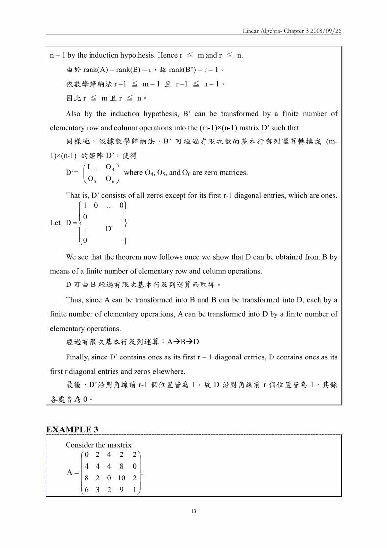
Linear Algebra- Chapter 3 20080926
16
rank(Dt) = r by Theorem 35
Thus
rank(At) = rank(Dt) = r = rank(A)
依據 Corollary 1存在可逆矩陣 B 與 C使得 D = BAC
取其轉置可得Dt = (BAC) t = CtAtBt
由於 B 與 C 為可逆故 Bt 與 Ct 亦為可逆
依據 Theorem 34得知 rank(At) = rank(CtAtBt) = rank(Dt)
設 r = rank(A)
則 Dt為一 ntimesm 的矩陣型式與 D 相同(參考 Corollary 1)
且依據 Theorem 35 得知 rank(Dt) = r
於是 rank(At) = rank(Dt) = r = rank(A)
Theorem 34 Let A be an mtimesn matrix If P and Q are invertible mtimesm and ntimesn matrices
respectively then 令 A 為 mtimesn 的矩陣若 P 與 Q 分別為可逆的 mtimesm 與 ntimesn 矩陣
則
(a) rank(AQ) = rank(A)
(b) rank(PA) = rank(A)
(c) rank(PAQ) = rank(A)
Theorem 35 The rank of any matrix equals the maximum number of its linearly
independent columns that is the rank of a matrix is the dimension of the subspace
generated by its column 任一矩陣的 Rank 等於其最大線性獨立行向量數目即矩陣
的 Rank 是由矩陣的行向量生成的子空間的維度【LA Fn Fm】
Corollary 3 Every invertible matrix is a product of elementary matrices
每一可逆矩陣均可為基本矩陣的乘積
【Proof】
If A is an invertible ntimesn matrix then rank(A) = n Hence the matrix D in Corollary 1
equals In and there exist invertible matrices B and C such that In = BAC
As in the proof of Corollary 1 note that B = EpEp-1hellipE2E1 and C = G1G2hellipGq where
the Eirsquos and Girsquos are elementary matrices Thus A = B-1InC-1 = B-1C-1 so that
A = E1-1E2
-1hellipEp-1Gq
-1Gq-1-1hellipG1
-1
Linear Algebra- Chapter 3 20080926
17
The inverses of elementary matrices are elementary matrices however and hence A is
the product of elementary matrices
若 A 為可逆的 ntimesn 矩陣則 rank(A) = n
因此 Corollary 1 中的矩陣 D 為 In且存在可逆的 B 與 C 矩陣使得 In = BAC
如同 Corollary 1 的證明一樣B = EpEp-1hellipE2E1 且 C = G1G2hellipGq其中Eirsquos 與
Girsquos 皆為基本矩陣
於是A = B-1InC-1 = B-1C-1即 A = E1-1E2
-1hellipEp-1Gq
-1Gq-1-1hellipG1
-1
基本矩陣的反矩陣亦為基本矩陣A 是基本矩陣的乘積
Theorem 37 Let T V W and U W Z be linear transformations on finite-dimensional vector
spaces V W and Z and let A and B be matrices such that the product AB is defined Then
令 VW 與 Z 為有限維度的向量空間T V W 與 U W Z 為線性轉換且
A 與 B 為滿足乘積 AB 定義的矩陣則
(a) rank(UT) ≦ rank(U)
(b) rank(UT) ≦ rank(T)
(c) rank(AB) ≦ rank(A)
(d) rank(AB) ≦ rank(B)
【Proof】
(a) Clearly R(T)subeW
Hence R(UT) = UT(V) = U(R(T)) sube U(W) = R(U)
Thus rank(UT) = dim(R(UT)) ≦ dim (R(U)) = rank(U)
(c) By (a) rank(AB) = rank(LAB) = rank (LALB) ≦ rank(LA) = rank(A)
(d) By (c) and Corollary 2 to Theorem 36
rank(AB) = rank((AB)t) = rank(B t A t) ≦ rank(B t) = rank (B) (b) Let α β and γ be ordered bases for V W and Z respectively and let Arsquo = γ
β]U[
and Brsquo = βα]T[ Then ArsquoBrsquo = γ
α]UT[ by Theorem 211
Hence by Theorem 33 and (d)
rank(UT) = rank(ArsquoBrsquo) ≦ rank(Brsquo) = rank (T)
Theorem 211 Let V W and Z be finite-dimensional vector space with ordered bases α β
and γ respectively Let T V W and U W Z be linear transformation Then
Linear Algebra- Chapter 3 20080926
18
βα
γβ
γα = [T][U][UT] 令 VW 與 Z 是有限維度的向量空間αβ 與 γ 分別為 VW 與
Z 的有序基底令 T V W (先 α β) 且 U W Z (後 β γ)則 βα
γβ
γα = [T][U][UT]
Theorem 33 Let T V W be a linear transformation between finite dimensional vector
spaces and let β and γ be ordered bases for V and W respective Then rank(T) = rank( γ
β[T] ) 令 T V W且 β 與 γ 分別為有限維度向量空間 V 與 W 的有序基底
則 rank(T) = rank( γβ[T] )
EXAMPLE 4
(a) Let ⎟⎟⎠
⎞⎜⎜⎝
⎛minus
=11111121
A (第一列與第二列是 LI) rank(A) = 2
(b) Let ⎟⎟⎟
⎠
⎞
⎜⎜⎜
⎝
⎛=
003011011131
A (第三列與第一二列是 LD)rank(A) = 2
(c) Let ⎟⎟⎟
⎠
⎞
⎜⎜⎜
⎝
⎛
minus=
011111121321
A (三列為 LI) rank(A) = 3
The inverse of a Matrix
We have remarked that an ntimesn matrix is invertible if and only if its rank is n Since we
know how to compute the rank of any matrix we can always test a matrix to determine
whether it is invertible We now provide a simple technique for computing the inverse of a
matrix that utilizes elementary row operations
已知 ntimesn 矩陣為可逆的『若且唯若』條件為該矩陣的 Rank 等於 n
DEFINITION 34 Augmented Matrix Let A and B be mtimesn and mtimesp matrices respectively By the augmented matrix )BA(
we mean that the mtimes(n+p) matrix )BA( that is the matrix whose first n columns are the
columns of A and whose last p columns are the columns of B 設 A 與 B 分別為 mtimesn 與 mtimesp 的矩陣則增廣矩陣(Augmented matrix) )BA(
Linear Algebra- Chapter 3 20080926
19
為一 mtimes(n+p)的矩陣 )BA( 該矩陣的前 n 行(Column)為 A 的所有的行後 p
行為 B 的所有行
Let A be an invertible ntimesn matrix and consider the ntimes2n augmented matrix C= )IA( n
C= )IA( n )AI()IAAA(CA 1
nn111 minusminusminusminus ==
By Corollary 3 to Theorem 36 A-1 is the product of elementary matrices say
A = EpEp-1hellipE2E1 (A-1 是多個基本矩陣的乘積)
Thus )AI()IAAA(CA 1
nn111 minusminusminusminus == )AI(CA)IA(EEE 1
n1
n11ppminusminus
minus ==
We have the following result If A is an invertible invertible ntimesn matrix then it is
possible to transform the matrix (AIn) into the matrix (InA-1) by means of a finite
number of elementary row operations
若 A 為一可逆的 ntimesn 矩陣則可經過有限次數的基本列運算將矩陣 (AIn) 化成
(InA-1)
Conversely suppose that A is invertible and that for some ntimesn matrix B the matrix
(AIn) can be transformed into the matrix (InB) by a finite number of elementary row
operations Let E1 E2hellip Ep be the elementary matrices associated with these elementary row
operations as in Theorem 31 then
反之假設 A 是可逆且矩陣(AIn)可經有限次數的基本列運算轉換成矩陣(InB)
並令 E1 E2hellip Ep 分別為 Theorem 31 所稱的基本矩陣則
)BI()IA(EEE nn11pp =minus
Let M = EpEp-1hellipE2E1 we have 令 M = EpEp-1hellipE2E1
)BI()IA(EEE nn11pp =minus )BI()IA(M)MMA( nn ==
Linear Algebra- Chapter 3 20080926
20
Hence MA = In and M = B It follows that M = A-1 So B = A-1
可由 MA = In 及 M = B 得知M 就是 A-1故 B 就是 A-1
Thus we have the follow resultsIf A is an invertible ntimesn matrix and the matrix
(AIn) is transformed in a matrix of the form (InB) by means of a finite number of
elementary row operations then B=A-1
若 A 為一可逆的 ntimesn 矩陣且矩陣 (AIn) 可經有限次數的基本列運算化成
(InB)則 B=A-1
If on the other hand A is an ntimesn matrix that is not invertible then rank(A) lt n Hence
any attempt to transform (AIn) into a matrix of the form (InB) by means of elementary row
operations must fail
反之若 A 是一不可逆的 ntimesn 矩陣則 rank(A) lt n因此任何想利用基本列運算
要將矩陣 (AIn) 化成 (InB)的努力必定失敗
Thus we have the follow results If A is an notinvertible ntimesn matrix then any attempt
to transform (AIn) into a matrix of the form (InB) produce a row whose first n entries
are zeros
若 A 是一不可逆的 ntimesn 矩陣任何想將矩陣 (AIn) 化成 (InB)的努力最後會
產生一前 n 個元素均為 0 的列
EXAMPLE 5
We determine whether the matrix ⎟⎟⎟
⎠
⎞
⎜⎜⎜
⎝
⎛=
133242420
A is invertible and if it is we
compute its inverse
A 是否為可逆矩陣
We attempt to use elementary row operations to transfer
Linear Algebra- Chapter 3 20080926
21
⎟⎟⎟
⎠
⎞
⎜⎜⎜
⎝
⎛=
100010001
133242420
)IA( into a matrix of the form (InB)
看看能否利用基本行與列運算將矩陣 (AIn) 化成 (InB)
Interchanging rows 1 and 2
⎟⎟⎟
⎠
⎞
⎜⎜⎜
⎝
⎛
100001010
133420242
Multiplying the first row by 12
⎟⎟⎟
⎠
⎞
⎜⎜⎜
⎝
⎛
10000100
133420121 2
1
Adding -3 times row 1 to row 3
⎟⎟⎟
⎠
⎞
⎜⎜⎜
⎝
⎛
minusminusminus 1000100
230420121
23
21
Multiplying row 2 by 12 to obtain 1 in the 22 position
⎟⎟⎟
⎠
⎞
⎜⎜⎜
⎝
⎛
minus
minus
minusminus 100000
230210121
23
21
21
Adding -2 times row 2 to row 1 and 3 times row 2 to row 3
⎟⎟⎟
⎠
⎞
⎜⎜⎜
⎝
⎛
minus
minusminus
10001
400210301
23
2321
21
Multiplying row 3 by 14
⎟⎟⎟
⎠
⎞
⎜⎜⎜
⎝
⎛
minus
minusminus
41
83
8321
21
0001
100210301
Adding appropriate multiply of row 3 to row 1 and 2 completes the process
⎟⎟⎟
⎠
⎞
⎜⎜⎜
⎝
⎛
minusminus
minus
41
83
83
21
43
41
43
85
81
100010001
目標達成
Thus A is invertible and ⎟⎟⎟
⎠
⎞
⎜⎜⎜
⎝
⎛
+minus+minus+minus+minus+
=minus
41
83
83
21
43
41
43
85
81
1A
Linear Algebra- Chapter 3 20080926
22
EXAMPLE 6
We determine whether the matrix ⎟⎟⎟
⎠
⎞
⎜⎜⎜
⎝
⎛minus=451112
121A is invertible and if it is we
compute its inverse
A 是否為可逆矩陣
We attempt to use elementary row operations to transfer
⎟⎟⎟
⎠
⎞
⎜⎜⎜
⎝
⎛minus=
100010001
451112
121)IA( into a matrix of the form (InB)
看看能否利用基本行與列運算將矩陣 (AIn) 化成 (InB)
Adding -2 times row 1 to row 2 and -1 times row 1 to row 3 then addig row 2 to row
3
⎟⎟⎟
⎠
⎞
⎜⎜⎜
⎝
⎛minus
100010001
451112
121
⎟⎟⎟
⎠
⎞
⎜⎜⎜
⎝
⎛
minusminusminusminus
101012001
330330
121
⎟⎟⎟
⎠
⎞
⎜⎜⎜
⎝
⎛
minusminusminusminus
113012001
000330
121
is a matrix with row whose first 3 entries are zeros Therefore A is not invertible
最後一列前 3 個元素均為 0
EXAMPLE 7 Let T P2(R) P2(R) be defined by T(f(x)) = f(x)+frsquo(x)+frdquo(x) where frsquo(x) and frdquo(x)
denote the first and second derivatives of f(x) We use Corollary 1 to Theorem 218 to test
T for invertibility and compute the inverse if T is invertible Taking β=1 x x2 to be the
standard ordered basis of P2(R) we have
令 T P2(R) P2(R) 為線性轉換且定義為 T(f(x)) = f(x)+frsquo(x)+frdquo(x)利用
Corollary 1 to Theorem 218 來測試 T 是否可逆並計算其逆轉換取 β=1 x x2為
P2(R)的標準有序基底
T(1) = 1 = 1bull1+0bullx+0bullx2
T(x) = 1+x = 1bull1+1bullx+0bullx2
Linear Algebra- Chapter 3 20080926
23
T(x2) = 2+2x+x2 = 2bull1+2bullx+1bullx2
⎟⎟⎟
⎠
⎞
⎜⎜⎜
⎝
⎛=β
100210211
[T] 稱為 T 相對有序基底 β的座標向量
依據 Corollary 1 to Theorem 218 T 可逆『若且唯若』 β[T] 可逆且
1-1 )[T](][T minusββ =
Using the method of Examples 5 and 6 we can show that β[T] is invertible with
inverse
⎟⎟⎟
⎠
⎞
⎜⎜⎜
⎝
⎛minus
minus=minus
β
100210
011)([T] 1
Thus T is is invertible and βminusminus
β = ][T)([T] 11 Hence by Theorem 214 we have
⎟⎟⎟
⎠
⎞
⎜⎜⎜
⎝
⎛minusminus
=⎟⎟⎟
⎠
⎞
⎜⎜⎜
⎝
⎛
⎟⎟⎟
⎠
⎞
⎜⎜⎜
⎝
⎛minus
minus=++ β
minus
2
21
10
2
1
02
2101
aa2aaa
aaa
100210
011)]xaxa(a[T
Therefore T-1(a0+a1x+a2x2) = (a0-a1)+(a1-2a2)x+a2x2 Corollary 1 to Theorem 218 Let V be finite-dimensional vector space with an ordered basis β and let T V V be linear Then T is invertible if and only if β[T] is invertible
Furthermore 1-1 )[T](][T minusββ = V 為有限維度的向量空間β 是 V 的有序基底令 T
V V 為線性轉換 T 為可逆的『若且唯若』條件為 β[T] 可逆再者
1-1 )[T](][T minusββ =
Theorem 214 Let V and W be finite-dimensional vector spaces having ordered bases β and γ respectively and let T V W be linear Then for each uisinV we have β
γβγ = [u][T][T(u)]
V 與 W 為有限維度的向量空間β 與 γ分別 V 與 W 的有序基底令 T V W 為線
性轉換則 V 中的 u 映至 W 的結果 T(u) 相對於有序基底 γ 的座標向量為
βγβγ = [u][T][T(u)]
Invertible and Inverse of MATRIX Let A be an n times n matrix If a matrix B can be found such that AB = BA = In then A is
Linear Algebra- Chapter 3 20080926
24
said to be invertible and B is called the inverse of A (denote B = A-1 and A-k=(A-1)k )
If such a matrix B does not exist then A has no inverse
EXAMPLE
⎥⎦
⎤⎢⎣
⎡=
4321
A and ⎥⎦
⎤⎢⎣
⎡minus
minus=
21
23
12B
221
23
221
23
I1001
432112
BA
I100112
4321
AB
=⎥⎦
⎤⎢⎣
⎡=⎥
⎦
⎤⎢⎣
⎡⎥⎦
⎤⎢⎣
⎡minus
minus=
=⎥⎦
⎤⎢⎣
⎡=⎥
⎦
⎤⎢⎣
⎡minus
minus⎥⎦
⎤⎢⎣
⎡=
Thus AB = BA = I2 proving that the matrix A has inverse B
Theorem The inverse of an invertible matrix is unique
Let B and C be inverse of A
Thus AB = BA = In and AC = CA = In
Multiply both sides of the equation AB = In by C
C(AB) = CIn (CA)B = C
InB = C B = C
Thus an invertible matrix has only one inverse
How to find AHow to find A--11
Based on the GaussBased on the Gauss--Jordan algorithmJordan algorithmLet A be an invertible matrix Then AALet A be an invertible matrix Then AA--11=I=Inn
Let the columns of Let the columns of AA--11 be be XX11 XX22 helliphellip XXnn and the columns of I and the columns of Inn be be CC11CC22helliphellipCCnn
Find AFind A--11 by finding by finding XX11 XX22 helliphellip XXnn Write the equation AAWrite the equation AA--11=I=Inn in the formin the form
[ ] [ ]n21nn211 CCCI XXXALet LL ==minus
[ ] [ ][ ] [ ]n21n21
n21n21
CCCAXAXXACCCXXXALL
LL
=rArr=
nn2211 CAXCAX CAX === LThus
How to find AHow to find A--11
Solving these systems by using Gauss-Jordan elimination on the large augmented matrix [AC1 C2hellipCn]
Thus when A-1 exits
[ ] [ ] [ ] 1n
1nn ABwhereBIAIIA minusminus ==asympasympL
If the reduced echelon form of [If the reduced echelon form of [AIAInn] is computed and ] is computed and the first part is not of the form Ithe first part is not of the form Inn then A has no inversethen A has no inverse
[ ][ ]n21n
n21
XXXI CCCAmatrix augmented
LL
L
asympasymp
Linear Algebra- Chapter 3 20080926
25
Example Example 1212
⎥⎥⎥
⎦
⎤
⎢⎢⎢
⎣
⎡
minusminusminusminusminus
=100531010532001211
]IA[ 3
⎥⎥⎦
⎤
⎢⎢⎣
⎡minusminusminus
minusminus
+minus+
asymp
101320012110001211
1RR1R3
2)(R2
⎥⎥⎦
⎤
⎢⎢⎣
⎡minus
minusminusminusasymp
101320012110001211
R2)1(
⎥⎥⎥
⎦
⎤
⎢⎢⎢
⎣
⎡
minusminusminusminusminus
=531532211
ADetermine the inverse of
Example Example 2222
⎥⎥⎦
⎤
⎢⎢⎣
⎡
minusminusminusminus
minus++asymp
123100012110013101
R2)2(R3R2R1
⎥⎥⎦
⎤
⎢⎢⎣
⎡
minusminusminus
minus++asymp
123100135010010001
R3)1(R2R3R1
123135110
A 1
⎥⎥⎥
⎦
⎤
⎢⎢⎢
⎣
⎡
minusminusminus=minus
⎥⎥⎦
⎤
⎢⎢⎣
⎡
minusminus
minus
+minus+asymp
135000011210012301
3R2R3R2)1(R1
ExampleExampleDetermine the inverse of
⎥⎥⎦
⎤
⎢⎢⎣
⎡
minus=
412721511
A
⎥⎥⎦
⎤
⎢⎢⎣
⎡
minus=
100412010721001511
][ 3IA
⎥⎥⎦
⎤
⎢⎢⎣
⎡
minusminusminusminus
minus+minus+asymp
102630011210001511
R1)2(R31)R1(R2
There is no need to proceed further There is no need to proceed further The reduced echelon form cannot have a one in the (3 3) locatioThe reduced echelon form cannot have a one in the (3 3) location n
The reduced echelon form cannot be of the form [IThe reduced echelon form cannot be of the form [Inn B] B] Thus Thus AAndashndash11 does not existdoes not exist
Properties of Matrix InverseProperties of Matrix Inverse
Let Let AA and and BB be invertible matrices andbe invertible matrices and cc a nonzero scalar a nonzero scalar ThenThen
AA =minusminus 11)( 111 1)( 2 minusminus = A
ccA
111)( 3 minusminusminus = ABAB
nn AA )()( 4 11 minusminus =tt AA )()( 5 11 minusminus =
Color Models Color Models 1212
A color model in the context of graphics is a method of A color model in the context of graphics is a method of implementing colorsimplementing colorsThe common used models include RGB model and YIQ modelThe common used models include RGB model and YIQ modelThe RGB model is used in computer monitors and the YIQ model The RGB model is used in computer monitors and the YIQ model is used in television screensis used in television screensAn RGB computer signal can be converted to a YIQ television An RGB computer signal can be converted to a YIQ television signal using the matrix transformationsignal using the matrix transformation
⎥⎥⎥
⎦
⎤
⎢⎢⎢
⎣
⎡
⎥⎥⎥
⎦
⎤
⎢⎢⎢
⎣
⎡
minusminusminus=
⎥⎥⎥
⎦
⎤
⎢⎢⎢
⎣
⎡
BGR
311523212321275596
114587299
QIY
YIQgtRGBYIQgtRGB
Color Models Color Models 2222
A signal is converted from a television screen to a computer monA signal is converted from a television screen to a computer monitor itor using inverse of the above matrixusing inverse of the above matrix
⎥⎥⎥
⎦
⎤
⎢⎢⎢
⎣
⎡
⎥⎥⎥
⎦
⎤
⎢⎢⎢
⎣
⎡
minusminusminus=
⎥⎥⎥
⎦
⎤
⎢⎢⎢
⎣
⎡rArr
⎥⎥⎥
⎦
⎤
⎢⎢⎢
⎣
⎡
⎥⎥⎥
⎦
⎤
⎢⎢⎢
⎣
⎡
minusminusminus=
⎥⎥⎥
⎦
⎤
⎢⎢⎢
⎣
⎡minus
QIY
0751108116472721
6209561
BGR
QIY
311523212321275596
114587299
BGR 1
CryptographyCryptography 密碼學密碼學 1212
Cryptography is the process of coding and decoding messagesCryptography is the process of coding and decoding messagesThe technique can be traced back to the ancient Greeks Today The technique can be traced back to the ancient Greeks Today governments use sophisticated methods of coding and decoding governments use sophisticated methods of coding and decoding messagesmessagesOne type of code that is extremely difficult to break makes use One type of code that is extremely difficult to break makes use of a of a large matrix to encode a message large matrix to encode a message The receiver of the message decodes it using the inverse of the The receiver of the message decodes it using the inverse of the matrixmatrixThe first matrix is called the encoding matrix and its inverse The first matrix is called the encoding matrix and its inverse is is called the decoding matrixcalled the decoding matrix
Cryptography Cryptography 密碼學密碼學 2222
A A-1Message
Encoding MatrixEncoding Matrix
Decoded MessageTransmission
Decoding MatrixDecoding Matrix
Linear Algebra- Chapter 3 20080926
26
Example Example 1212
Let the message be Let the message be BUY IBM STOCKBUY IBM STOCKAnd the encoding matrix beAnd the encoding matrix be
⎥⎥⎥
⎦
⎤
⎢⎢⎢
⎣
⎡ minusminusminus
434110433
B U Y B U Y -- I B M I B M -- S T O C KS T O C K2 21 25 27 9 2 13 27 19 20 15 3 112 21 25 27 9 2 13 27 19 20 15 3 11
⎥⎥⎥
⎦
⎤
⎢⎢⎢
⎣
⎡ minusminusminusminusminus=
⎥⎥⎥
⎦
⎤
⎢⎢⎢
⎣
⎡
⎥⎥⎥
⎦
⎤
⎢⎢⎢
⎣
⎡ minusminusminus
2331372091431715418461146
222117196116169
27319225271527921112013272
434110433
EncodingEncoding
Example Example 2222
Let the message be Let the message be BUY IBM STOCKBUY IBM STOCKAnd the decoding matrix beAnd the decoding matrix be
⎥⎥⎥
⎦
⎤
⎢⎢⎢
⎣
⎡
minusminus 334344101
B U Y B U Y -- I B M I B M -- S T O C KS T O C K2 21 25 27 9 2 13 27 19 20 15 3 112 21 25 27 9 2 13 27 19 20 15 3 11
⎥⎥⎥
⎦
⎤
⎢⎢⎢
⎣
⎡=
⎥⎥⎥
⎦
⎤
⎢⎢⎢
⎣
⎡ minusminusminusminusminus
⎥⎥⎥
⎦
⎤
⎢⎢⎢
⎣
⎡
minusminus 27319225271527921112013272
2331372091431715418461146
222117196116169
334344101
DecodingDecoding
3-3 Systems of Linear Equations ndash Theoretical Aspects
The system of equations
mnmn22m11m
2nn2222121
1nn1212111
bxaxaxa
bxaxaxabxaxaxa
=+++
=+++=+++
(S)
were aij and bi (1≦i≦m and 1≦j≦n) are scalars in a field F and x1 x2hellipxn are n
variables taking values in F is called a system of m linear equations in n unknows over the
field F
上式稱為佈於 Field F 含有 n 個未知數m 個線性方程式的系統或方程組(system
of m linear equations in n unknows)
The mtimesn matrix
⎟⎟⎟⎟⎟
⎠
⎞
⎜⎜⎜⎜⎜
⎝
⎛
=
mn2m1m
n22221
n11211
aaa
aaaaaa
A is called the coefficient matrix of the
system (S)(係數矩陣) If we let
⎟⎟⎟⎟⎟
⎠
⎞
⎜⎜⎜⎜⎜
⎝
⎛
=
n
2
1
x
xx
x and
⎟⎟⎟⎟⎟
⎠
⎞
⎜⎜⎜⎜⎜
⎝
⎛
=
m
2
1
b
bb
b Then the system (S) may
be rewritten as a single matrix equation Ax = b(單一矩陣方程式)
To exploit the results that we have developed we often consider a system of linear
equations as a single matrix equation
Linear Algebra- Chapter 3 20080926
27
A solution to the system (S) is an n-tuple n
n
2
1
F
s
ss
s isin
⎟⎟⎟⎟⎟
⎠
⎞
⎜⎜⎜⎜⎜
⎝
⎛
= such that As = b The set of
all solutions to the system (S) is called the solution set of the system(解集合) System (S)
is called consistent(相容) if its solution set is nonempty otherwise it is called
inconsistent(不相容)
方程組(S)的解為一 n 序組該序組可以使 As = b方程組的所有解所成的集合
稱為該方程組的解集合(Solution set)方程組的解集合非空集合者稱為「相容」解
集合空集合者稱為「不相容」
EXAMPLE 1
Consider 6x2xx1xx3x2
321
321
=+minus=++
that is ⎟⎟⎠
⎞⎜⎜⎝
⎛=
⎟⎟⎟
⎠
⎞
⎜⎜⎜
⎝
⎛
⎟⎟⎠
⎞⎜⎜⎝
⎛minus 6
1
xxx
211132
3
2
1
(以矩陣表示)
This system has many solutions such as ⎟⎟⎟
⎠
⎞
⎜⎜⎜
⎝
⎛minus=
726
s and ⎟⎟⎟
⎠
⎞
⎜⎜⎜
⎝
⎛
minusminus=
34
8s
Consider 1xx0xx
21
21
=+=+
that is ⎟⎟⎠
⎞⎜⎜⎝
⎛=⎟⎟
⎠
⎞⎜⎜⎝
⎛⎥⎦
⎤⎢⎣
⎡10
xx
1111
2
1
顯然地方程組無解
We begin our study of system of linear equations by examining the class of
homogeneous system of linear equations 先討論齊次方程組
DEFINITION 35 Homogeneous amp Nonhomogeneous
A system Ax=b of m linear equations in n unknowns is said to be homogeneous if b=0
Otherwise the system is said to be nonhomogeneous
方程組 Ax = bb = 0 稱為齊次方程組否則稱為非齊次方程組
Any homogeneous system has at least one solution namely the zero vector The next
result gives further information about the set of solutions to a homogeneous system
Linear Algebra- Chapter 3 20080926
28
齊次方程組至少有一個解那就是『零向量』
Theorem 38 Let Ax = 0 be a homogeneous system of m linear equations in n unknowns over a field
F Let K denote the set of all solutions to Ax = 0 Then K = N(LA) hence K is a subspace
of Fn of dimension n - rank(LA) = n- rank(A)
令 Ax = 0 代表一佈於 Field 含有 n 個未知數m 個線性方程式的方程組若令
K 代表該方程組的解集合(Solution set)則 K = N(LA)K 為 Fn 內的子空間且其維
度為 n ndash rank (LA) = n - rank(A)
【Proof】
Clearly K = sisinFn As = 0 = N(LA) The second part now follows from the
dimension theorem
Nullity(T)+rank(T) = dim(V)
Nullity (LA) = dim (Fn) ndashrank (LA ) = n ndash rank (A)
DEFINTION 27 Let V and W be vector space and let T V W be linear We define
the null space (or kernel) N(T) of T to be the set of all vectors x in V such that T(x) = 0
that is N(T) = xisinV T(x) = 0 V 與 W 為向量空間且 T V W 為線性轉換定義
線性轉換 T 的 Null space 為 V 內所有滿足 T(x) = 0 的向量 x 所形成的集合註記為
N(T)Null space 的元素 x 經線性轉換 T 轉換後所對應的「像」為 0意即 T(x) = 0
Null space 內的元素的「像」皆為 0
DEFINITION 217 Let A be an mtimesn matrix with entries from a field F We denote by LA
the mapping LA Fn Fm defined by LA(x) = Ax (the matrix product A and x) for each
column vector xisinFn We call LA a left-multiplication transformation 令 A 是 mtimesn
的矩陣所有元素均來自 FLA 為 Fn 映至 Fm的線性轉換並定義為 LA(x) = Ax其中
x 為行向量(Column vector)且 xisinFnLA被稱為左乘法轉換
Theorem 23 (Dimension Theorem) Let V and W be vector spaces and let T V W be
linear If V is finite-dimensional then Nullity(T) + rank(T) = dim(V) T 的核次數
(Nullity)與秩(Rank)的和等於定義域的維度 dim(V)
Corollary Let Ax = 0 be a homogeneous system of m linear equations in n unknowns over a field
Linear Algebra- Chapter 3 20080926
29
F If m lt n the system Ax = 0 has a nonzero solution
令 Ax = 0 代表一佈於 Field 含有 n 個未知數m 個線性方程式的方程組若 m
lt n則該方程組具有一非零解
【Proof】
Suppose that m lt n Then rank(A) = rank (LA)≦m Hence dim(K) = n - rank(LA) ≧
n ndash m gt 0 where K = N(LA) Since dim(K) gt 0 Kne 0 Thus there exists a nonzero
vector sisinK so s is a nonzero solution to Ax = 0
設 m lt n則 rank(A) = rank (LA) ≦ m依據 Theorem 38K = sisinFn As = 0
= N(LA) = dim(K) = n - rank(LA) ≧ n ndash m gt 0表示 dim(K) gt 0Kne 0故存在非
零向量 s使得 Ax = 0
EXAMPLE 2
Consider 0xxx
0xx2x
321
321
=minusminus=++
Let ⎟⎟⎠
⎞⎜⎜⎝
⎛minusminus
=111
121A be the coefficient matrix of this system It is clear that rank(A)
= 2 If K is the solution set of this system then dim(K) = 3-2 = 1 Thus any nonzero
solution constitutes a basis for K
若 K 是方程組的解所組成的集合(簡稱為解集合)依 Theorem 38 得知 dim(K)
= 3 - 2 = 1因此任一非零解將形成 K 的基底
For example since ⎟⎟⎟
⎠
⎞
⎜⎜⎜
⎝
⎛minus32
1 is a solution to the given system
⎪⎭
⎪⎬
⎫
⎪⎩
⎪⎨
⎧
⎟⎟⎟
⎠
⎞
⎜⎜⎜
⎝
⎛minus32
1 is a basis for
K Thus any vector in K is of the form ⎟⎟⎟
⎠
⎞
⎜⎜⎜
⎝
⎛minus=
⎟⎟⎟
⎠
⎞
⎜⎜⎜
⎝
⎛minus
t3t2
t
32
1t where tisinR
例如因⎟⎟⎟
⎠
⎞
⎜⎜⎜
⎝
⎛minus32
1是方程組的一個解故
⎪⎭
⎪⎬
⎫
⎪⎩
⎪⎨
⎧
⎟⎟⎟
⎠
⎞
⎜⎜⎜
⎝
⎛minus32
1 為 K 的基底K 內的任一向量均
具有如下形式
⎟⎟⎟
⎠
⎞
⎜⎜⎜
⎝
⎛minus=
⎟⎟⎟
⎠
⎞
⎜⎜⎜
⎝
⎛minus
t3t2
t
32
1t
Linear Algebra- Chapter 3 20080926
30
We now turn to the study of nonhomogeneous systems Our next result shows that the
solution set of a nonhomogeneous system Ax = b can be described in terms of the solution of
the homogeneous system Ax = 0 We refer to the equation Ax = 0 as the homogeneous system
corresponding to Ax = b
以下將進一步探討「非齊次方程組」非齊次方程組 Ax = b 的解集合可利用齊次方
程組 Ax = 0 的解來加以說明因此我們可將 Ax = 0 視為 Ax = b 的齊次方程組
Theorem 39 Let K be the solution set of a system of linear equations Ax = b and let KH be the
solution set of the corresponding homogeneous system Ax = 0 Then for any solution s to
Ax = b K =s + KH = s+k kisinKH
設 K 為線性方程組 Ax = b 的解集合且 KH為對應的齊次方程組的解集合則
對 Ax = b 的任一個解 s 而言K =s + KH = s+k kisinKH
【Proof】
Let s be any solution to Ax = b
We must show that K =s + KH
If wisinK then Aw = b Hence
A(w - s) = Aw ndash As = b ndash b = 0
So w - sisinKH
Thus there exists kisinKH such that w - s = k
It follows that w = s + k isin s +KH and therefore Ksube s +KH
Conversely suppose that wisins +KH then w = s + k for some kisinKH
But then Aw = A(s + k) = As + Ak = b + 0 = b so wisinK
Therefore s +KHsubeK and thus K=s +KH
令 s 為 Ax = b 的任一個解我們必須證明「K =s + KH」
若 wisinK則 Aw = b(即 w 為 Ax = b 的解)
於是 A(w - s) = Aw ndash As = b ndash b = 0
所以 w - sisinKH(即 w-s 為 Ax = 0 的解)
w - s 既然是 KH的元素表示有一元素 kisinKH使得 w - s = kw = s + k
w = s + kisins +KH
Linear Algebra- Chapter 3 20080926
31
因此 Ksube s +KH
反之假設 wisins +KH則 KH中存在一元素 k(kisinKH)使得 w = s + k
因 Aw = A(s + k) = As + Ak = b + 0 = b
故 wisinK 是 Ax = b 的解
因此s +KHsubeK
總結K=s +KH
EXAMPLE 3
Consider 4xxx7xx2x
321
321
minus=minusminus=++
The corresponding homogeneous system is the system in Example 2 It is easily
verified that ⎟⎟⎟
⎠
⎞
⎜⎜⎜
⎝
⎛=
411
s is a solution to the preceeding nonhomogeneous system So the
solution set of the system is ⎪⎭
⎪⎬
⎫
⎪⎩
⎪⎨
⎧isin
⎟⎟⎟
⎠
⎞
⎜⎜⎜
⎝
⎛minus+
⎟⎟⎟
⎠
⎞
⎜⎜⎜
⎝
⎛= Rt
32
1t
411
K by Theorem 39
⎟⎟⎟
⎠
⎞
⎜⎜⎜
⎝
⎛=
411
s 是非齊次方程組 Ax = b 的解
⎟⎟⎟
⎠
⎞
⎜⎜⎜
⎝
⎛minus32
1是齊次方程組的解
依據 Theorem 39 得知線性方程組 Ax = b 的解集合⎪⎭
⎪⎬
⎫
⎪⎩
⎪⎨
⎧isin
⎟⎟⎟
⎠
⎞
⎜⎜⎜
⎝
⎛minus+
⎟⎟⎟
⎠
⎞
⎜⎜⎜
⎝
⎛= Rt
32
1t
411
K
The following theorem will provide us with a means of computing solutions to certain
system of linear equations
Theorem 310~311 提供計算線性方程組的解的方法
Theorem 310 Let Ax = b be a system of n linear equations in n unknowns If A is invertible then the
Linear Algebra- Chapter 3 20080926
32
system has exactly one solution namely A-1b Conversely if the system has exactly one
solution then A is invertible
令 Ax = b 為含 n 個未知數n 個線性方程式的方程組若 A 為可逆則方程組
恰有一個解解為 A-1b反之若該方程組恰有一個解則 A 為可逆
【Proof】
Suppose that A is invertible
Substituting A-1b into system we have A(A-1b)=( AA-1)b = b
Thus A-1b is a solution
If s is an arbitrary solution then As = b
Multiplying both sides by A-1 gives s= A-1b
Thus the system has one and only one solution namely A-1b
假設 A 為可逆將 A-1b 代入方程組可得 A(A-1b)=( AA-1)b = b
故 A-1b 確為方程組的解
若 s 為方程組的任意解則 As = b
兩邊乘上 A-1可得 s= A-1b
因此方程組僅有唯一的解 A-1b
Conversely suppose that the system has exactly one solution s
Let KH denot the solution set for the corresponding homogeneous system Ax = 0
By Theorem 39 s = s + KH But it is so only if KH = 0 Thus N(LA) = 0 and
hence A is invertible
反之假設方程組恰有一個解 s
令 KH為相對應齊次方程組 Ax = 0 的解集合
依據 Theorem 39要能s = s + KH唯有 KH = 0
KH = 0即表示 N(LA) = 0故 A 為可逆
EXAMPLE 4 Consider the following system of three linear equations in three unknowns
1xx3x33x2x4x2
2x4x2
321
321
32
=++=++
=+
In Example 5 of Section 32 we compute the inverse of the coefficient matrix A of
this system Thus the system has exactly one solution namely
Linear Algebra- Chapter 3 20080926
33
⎟⎟⎟
⎠
⎞
⎜⎜⎜
⎝
⎛=
133242420
A⎟⎟⎟
⎠
⎞
⎜⎜⎜
⎝
⎛
+minus+minus+minus+minus+
=minus
41
83
83
21
43
41
43
85
81
1A
⎟⎟⎟
⎠
⎞
⎜⎜⎜
⎝
⎛
minus+minus
=⎟⎟⎟
⎠
⎞
⎜⎜⎜
⎝
⎛
⎟⎟⎟
⎠
⎞
⎜⎜⎜
⎝
⎛
+minus+minus+minus+minus+
==⎟⎟⎟
⎠
⎞
⎜⎜⎜
⎝
⎛minus
814587
41
83
83
21
43
41
43
85
81
1
3
2
1
132
bAxxx
Theorem 311 Let Ax = b be a system of linear equations Then the system is consistent (相容)if
and only if rank(A) = rank (A∣b) Matrix (A b) is called the augmented matrix o∣ f the
system Ax = b
令 Ax = b 為線性方程式方程組則此方程組至少有一個解的『若且唯若』條件
為 rank(A) = rank (A∣b) 矩陣(A∣b)稱為方程組 Ax = b 的增廣矩陣
【Proof】
To say that Ax = b has a solution is equivalent to saying that bisinR(LA)
In the proof of Theorem 35 we saw that R(LA ) = span(a1 a2 an) the span of the
column of A
Thus Ax = b has a solution if and only if bisinspan(a1 a2 an)
But bisinspan(a1 a2 an) if and only if span(a1 a2 an) = span(a1 a2 an b)
This last statement is equivalent to
dim (span(a1a2an)) = dim (span(a1a2an b))
So by Theorem 35 the preceeding equation reduces to rank(A) = rank (A∣b)
Ax = b 有一解相當於 bisinR(LA)即 b 屬於線性轉換 LA的 Range
在 Theorem 35 的證明中提到 R(LA ) = span(a1a2an)aj 為 A 的第 j 個行
(Column)即線性轉換 LA 的 Range 係由矩陣 A 的行(Column)所生成
因此 Ax = b 要有一個解的『若且唯若』條件為 bisinspan(a1 a2 an)
至於 bisinspan(a1 a2 an)之條件
bisinspan(a1a2an) 的『若且唯若』條件為 span(a1a2an) = span(a1a2an
b)
其條件相當於
Linear Algebra- Chapter 3 20080926
34
dim (span(a1a2an)) = dim (span(a1a2an b))
依據 Theorem 35該條件可簡化為 rank(A) = rank (A∣b)
Theorem 35 The rank of any matrix equals the maximum number of its linearly
independent columns that is the rank of a matrix is the dimension of the subspace
generated by its column任一矩陣的 Rank 等於其最大線性獨立行向量數目即矩陣的
Rank 是由矩陣的行向量生成的子空間的維度【LA Fn Fm】
EXAMPLE 5 Recall the system of equations
1xx0xx
21
21
=+=+
Since ⎟⎟⎠
⎞⎜⎜⎝
⎛=
1111
A and ⎟⎟⎠
⎞⎜⎜⎝
⎛=
111011
)bA(
rank(A) = 1 and rank (A b) = 2∣
Because the two ranks are unequal the system has no solutions
矩陣 A 與增廣矩陣(A∣b) 的 Rank 不同故方程組沒有解
EXAMPLE 6 We can use Theorem 311 to determine whether (3 3 2) is in the range of the linear
transformation T R3 R3 defined by T(a1 a2 a3) = (a1+a2+a3 a1-a2+a3 a1+a3)
利用 Theorem 311 來判斷 (3 3 2)是否在線性轉換 T 的 Range 中其中T R3
R3 定義為 T(a1 a2 a3) = (a1+a2+a3 a1-a2+a3 a1+a3)
Now (3 3 2)isinR(T) if and only if there exists a vector s = x1 x2 x3 in R3 such that
T(s)=(3 3 2) Such a vector s must be a solution to the system
2xx3xxx3xxx
31
321
321
=+=+minus=++
Since the ranks of the coefficient matrix and the augmented matrix of this system
are 2 and 3 respectively it follows that this system has no solutions Hence (3 3 2) notin
R(T)
(3 3 2)isinR(T) 的『若且唯若』的條件為存在一向量 s = x1 x2 x3isinR3 使得
T(s)=(3 3 2)
Linear Algebra- Chapter 3 20080926
35
向量 s 必須是 2xx3xxx3xxx
31
321
321
=+=+minus=++
的解
因係數矩陣⎟⎟⎟
⎠
⎞
⎜⎜⎜
⎝
⎛minus
101111111
的 Rank 為 2增廣矩陣⎟⎟⎟
⎠
⎞
⎜⎜⎜
⎝
⎛minus
233
101111111
的 Rank 為 3兩
者不相等故方程組無解(3 3 2) notin R(T)
Theorem 311 Let Ax = b be a system of linear equations Then the system is consistent
(相容)if and only if rank(A) = rank (A∣b) Matrix (A b) is called the ∣ augmented
matrix of the system Ax = b 令 Ax = b 為線性方程式方程組則此方程組至少有一個
解的『若且唯若』條件為 rank(A) = rank (A∣b) 矩陣(A∣b)稱為方程組 Ax = b 的
增廣矩陣
Application
In 1973 Wassily Leontief won the Nobel prize in economics for his work in developing
a mathematical model that can be used to describe various economic phenomena
1973 年Wassily Leontief 因研究一數學模式來描述各種經濟現象而獲頒諾貝爾經
濟獎
CLOSED MODEL
We begin by considering a simple society composed of three peoples (industries) ndash a
farmer who gows all the food a tailor who makes all the clothing and a carpenter who builds
all the housing We assume that each person sells to and buy from a central pool and that
everything produced is consumed Since no commodities either enter or leave the system this
case is referred to as the CLOSE MODEL
考慮一個單純社會的三種人生產食物的農夫製衣的裁縫師與蓋住屋的木匠
並假設採取集中聯營買賣且每一件產品皆付諸消費由於過程中沒有任何成品進入
或脫離這個系統所以稱為「封閉模式」
Each of these three individual consumes all three of the commodities produced in the
Linear Algebra- Chapter 3 20080926
36
society Suppose that the proportion of each of the commodities consumed by each person is
given in the following table
社會中每一位皆消費所生產的三種成品且每一種產品也都被三位所消費其消
費比例如下
食物 Food 衣物 Clothing 住屋 Housing
農夫 Farmer 040 020 020
裁縫師 Tailor 010 070 020
木匠 Carpenter 050 010 060
Let p1 p2 and p3 denote the incomes of the farmer tailor and carpenter respectively To
ensure that this society survives we require that the consumption of each individual equals
his or her income
令 p1p2 與 p3 分別表示農夫裁縫師與木匠的收入並為確保這個封閉社會可以
存活假設每一位的收入等於消費
Note that the farmer consumes 20 of the clothing Because the total cost of all clothing
is p2 the tailorrsquos income the amount spent by the farmer on clothing is 020 p2 Moreover the
amount spent by the farmer on food clothing and housing must equal the farmerrsquos income
and so we obtain the equation 040 p1 + 020 p2 + 030 p3 = p1
對農夫而言農夫的衣物消費佔 20然因所有衣物的消費總額 p2 等於裁縫師的
收入所以農夫在衣物上的消費為 020 p2且農夫在食物衣物與住屋的總消費要等
於農夫的收入 p1所以農夫的收入與消費關係式
040 p1 + 020 p2 + 020 p3 = p1
Similary equations describing the expenditures of the tailor and carpenter produce the
following system of linear equations
同理分別對裁縫師與木匠進行討論可獲得下列方程組
Linear Algebra- Chapter 3 20080926
37
040 p1 + 020 p2 + 020 p3 = p1
010 p1 + 070 p2 + 020 p3 = p2
050 p1 + 010 p2 + 060 p3 = p3
This system can be written as Ap = p
其中⎟⎟⎟
⎠
⎞
⎜⎜⎜
⎝
⎛=
3
2
1
ppp
p 且⎟⎟⎟
⎠
⎞
⎜⎜⎜
⎝
⎛=
600100500200700100200200400
A 稱為輸入-輸出(或消費)矩陣
(Input-output (or consumption) matrix)
Ap = p 稱為均衡條件(Equilibrium condition)
能否利用不等式 p ≦ p 來替代等式
At first it may seem reasonable to replace the equilibrium condition by the inequality
Ap ≦ p that is the requirement that consumption not exceed production But in fact Ap ≦ p implies that Ap = p in the closed model
For otherwise there exists a k for which
sumgt
jjkjk pAp
Hence since the columns of A sum to 1
sumsumsumsum ==gt
jj
i jjij
ii ppAp which is a contradiction (出現矛盾)
答案是在封閉系統中Ap ≦ p Ap = p
One solution to the homogeneous system (I ndash A) x = 0 which is equivalent to the
equilibrium condition is ⎟⎟⎟
⎠
⎞
⎜⎜⎜
⎝
⎛=
400350250
p
Linear Algebra- Chapter 3 20080926
38
齊次方程組(I ndash A) x = 0 或均衡條件的一個解為 ⎟⎟⎟
⎠
⎞
⎜⎜⎜
⎝
⎛=
400350250
p
We may interpret this to mean that the society survives if the farmer taior and carpenter
have incomes in the proportions 253540
⎟⎟⎟
⎠
⎞
⎜⎜⎜
⎝
⎛=
400350250
p 可以解釋為若農夫裁縫師與木匠收入比例為 253540則社會將
能生存下去
Theorem 312
Let A be an ntimesn input-output matrix having the form ⎟⎟⎠
⎞⎜⎜⎝
⎛=
EDCB
A where D is a 1times(n-
1) positive vector and C is an (n-1)times1 positive vector Then (I-A)x = 0 has a one-
dimensional solution set that is generated by a nonnegative vector
設 A 為 ntimesn 輸入-輸出矩陣 ⎟⎟⎠
⎞⎜⎜⎝
⎛=
EDCB
A 其中D 為 1times(n-1)正向量C 為
(n-1)times1 正向量則(I-A)x = 0 具有一維解集合且該解集合係由一非負向量所生成
Any input-output matrix with all positive entries satisfies the hypothesis of this theorem
任何輸入-輸出矩陣滿足 Theorem 312 的基本假設條件例如
⎟⎟⎟
⎠
⎞
⎜⎜⎜
⎝
⎛=
02502503502500650500750
A
OPEN MODEL
In the OPEN MODEL we assume that there is an outside demand for each of the
commodities produced Returning to our simple society let x1 x2 and x3 be the monetary
values of food clothing and housing produced with respective outside demands d1 d2 and d3
Let A be the 3times3 matrix such that Aij represents the amount of commodity i required to
Linear Algebra- Chapter 3 20080926
39
produce one monetary unit of commodity j Then the value of the surplus of food in the
society is x1 ndash (A11x1+A12x2+A13x3) that is the value of food produced minus the value of
food consumed while producing the three commodities The assumption that everything
produced is consumed gives us a similar equilibrium condition for the open model namely
that the surplus of each of the three commodities must equal the corresponding outside
demands Hence i
3
1jjiji dxAx =minussum
=
for j=1 2 3
在「開放模式」中我們假設每一產品皆有外來的需求在前述的單純社會裡
令 x1x2 與 x3 分別代表食物衣物與住屋的貨幣價值d1d2 與 d3 為食物衣物與住
屋的外來需求價值令 A 為 3times3 矩陣Aij 表示生產『一個貨幣單位』的產品 j 所需要
的產品 i 的價值於是此社會中食物的盈餘價值為 x1 ndash (A11x1+A12x2+A13x3)即食物的
價值減去生產食物衣物與住屋所需消耗的食物的價值意即生產出來的食物價值扣
掉用去生產食物衣物與住屋所消耗掉的價值)(A11A12A13 為生產一個貨幣單位
的食物 1衣物 2 與住屋 3 所需消耗的食物 1 數量A12x2 表示生產貨幣價值為 x2的衣物
所需要的食物價值)對每一種產品而言其盈餘價值等於外來的需求價值於是
i
3
1jjiji dxAx =minussum
=
for j=123
Suppose that 30 cents worth of food 10 cents worth of clothing and 30 cents worth of
housing are required for the production of $1 worth of food Similar suppose that 20 cents
worth of food 40 cents worth of clothing and 20 cents worth of housing are required for the
production of $1 worth of clothing Finally suppose that 30 cents worth of food 10 cents
worth of clothing and 30 cents worth of housing are required for the production of $1 worth
of housing Then the input-output matrix is
⎟⎟⎟
⎠
⎞
⎜⎜⎜
⎝
⎛=
300200300100400100300200300
A
假設生產價值 1 元的食物需要價值 30 分的食物(A11 = 03)價值 10 分的衣物
(A21 = 01)及價值 30 分的住屋(A31 = 03)生產價值 1 元的衣物需要價值 20 分的
食物(A12 = 02)價值 40 分的衣物(A22 = 04)及價值 20 分的住屋(A32 = 02)生
Linear Algebra- Chapter 3 20080926
40
產價值 1 元的住屋需要價值 30 分的食物(A13 = 03)價值 10 分的衣物(A23 = 01)
及價值 30 分的住屋(A33 = 03)於是輸入輸出矩陣 A 為
⎟⎟⎟
⎠
⎞
⎜⎜⎜
⎝
⎛=
300200300100400100300200300
A
若食物的外來需求值為 300 億元衣物為 200 億元住屋值為 1 百億元則
⎟⎟⎟
⎠
⎞
⎜⎜⎜
⎝
⎛=
⎟⎟⎟
⎠
⎞
⎜⎜⎜
⎝
⎛
⎟⎟⎟
⎠
⎞
⎜⎜⎜
⎝
⎛
minusminusminusminusminusminus
=minus=
minus
minus
700600900
100200300
700200300100600100300200300
d)AI(x
1
1
⎟⎟⎟
⎠
⎞
⎜⎜⎜
⎝
⎛=
700600900
x 表示要滿足外來需求必須生產的食物價值為 900 億元衣物價值為
600 億元住屋價值為 700 億元
Theorem
Let AX = Y be a system of n linear equations in n variables If Andash1 exists the
solution is unique and is given by X = Andash1Y
【Proof】
Substitute X = Andash1Y into the matrix equation
AX = A(Andash1Y) = (AAndash1)Y = InY = Y
The solution is unique
Let X1 be any solution thus AX1 = Y Multiplying both sides of this equation by Andash1
gives
Andash1AX1= Andash1Y InX1 = Andash1Y X1 = Andash1Y
Linear Algebra- Chapter 3 20080926
41
Example Example 1212
2x5x3x3x5x3x21x2x x
321
321
321
minus=++minus=minusminus=minusminus
⎥⎥⎥
⎦
⎤
⎢⎢⎢
⎣
⎡
minus=
⎥⎥⎥
⎦
⎤
⎢⎢⎢
⎣
⎡
⎥⎥⎥
⎦
⎤
⎢⎢⎢
⎣
⎡
minusminusminusminusminus
231
xxx
531532211
3
2
1
Solve the system of equations
This system can be written in the following matrix form
⎥⎥⎥
⎦
⎤
⎢⎢⎢
⎣
⎡
minus⎥⎥⎥
⎦
⎤
⎢⎢⎢
⎣
⎡
minusminusminusminusminus
=
⎥⎥⎥
⎦
⎤
⎢⎢⎢
⎣
⎡minus
231
531532211
xxx 1
3
2
1
If the matrix of coefficients is invertible the unique solutionIf the matrix of coefficients is invertible the unique solution isis
Example Example 2222
1 2 1 issolution unique The 321 =minus== xxx
⎥⎥⎥
⎦
⎤
⎢⎢⎢
⎣
⎡minus=
⎥⎥⎥
⎦
⎤
⎢⎢⎢
⎣
⎡
minus⎥⎥⎥
⎦
⎤
⎢⎢⎢
⎣
⎡
minusminusminus=
⎥⎥⎥
⎦
⎤
⎢⎢⎢
⎣
⎡
121
231
123135110
xxx
3
2
1
⎥⎥⎥
⎦
⎤
⎢⎢⎢
⎣
⎡
minusminusminus=
⎥⎥⎥
⎦
⎤
⎢⎢⎢
⎣
⎡
minusminusminusminusminus
=
minus
minus
123135110
531532211
A
1
1
The The LeontiefLeontief IO Model in IO Model in Economics Economics 1515
The Leontief input-output model is used to analyze the interdependence of economics Wassily Leontief received a Nobel Prize in 1973 for his work in thie fieldThe practical applications of this model have proliferated until it has now become a standard tool for investigating economic structures ranging from cities and corporation to states and countriesConsider an economics situation that involves ninterdependent industries The output of any one industry is needed as input by other industries and even possibly by the industry itself
The The LeontiefLeontief IO Model in IO Model in Economics Economics 2525
How a mathematical model involving a system of linear equations can be constructed to analyze such a situationAssume that each industry produces one commodity Let aij denote the amount of input of a certain commodity i to produce unit output of commodity j In our model let the amounts of input and output be measured in dollars Thus for example a34 = 045 means that 45 centsrsquo worth of commodity 3 is required to produce one dollarrsquos worth of commodity 4
The The LeontiefLeontief IO Model in IO Model in Economics Economics 3535
aij = amount of commodity i in one dollar of commodity jaij =生產一元價值的j產品需要耗用的i產品價值
The elements aij called input coefficients define a matrix A called the input-output matrix which describes the interdependence of the industriesExtending the model to include an open sector (all non-producing sectors) The product of industries may go not only into other producing industries but also into other non-producing sectors of the economy such as consumers and governments
The The LeontiefLeontief IO Model in IO Model in Economics Economics 4545
di = demand of the open sectors from industry ixi=total output of industry I necessary to meet demands of all n industries and the open sector
sectoropen of demand
nindustry of demand
2industry of demand
22
1industry of demand
11
industry ofoutput total
ininii
i
i dxaxaxax ++sdotsdotsdot++=
output ofportion sectoropen
output ofportion tryinterindusoutput total
DAXX +=Demand matrixDemand matrix
Output matrixOutput matrix
The The LeontiefLeontief IO Model in IO Model in Economics Economics 5555
Applying the model to the economy of a country X Applying the model to the economy of a country X represents the total output of each of the producing sectors represents the total output of each of the producing sectors of the economy and AX describes the contributions made of the economy and AX describes the contributions made by the various sectors to fulfilling the intersectional input by the various sectors to fulfilling the intersectional input requirements of the economyrequirements of the economyD is equal to (XD is equal to (X--AX) the difference between total output AX) the difference between total output X and industry transaction AXX and industry transaction AXD is thus the gross national product of the economyD is thus the gross national product of the economy
Example Example 1414
Consider an economy consisting of three industries having Consider an economy consisting of three industries having the following inputthe following input--output matrix output matrix AA Determine the output Determine the output levels required of the industries to meet the demands of levels required of the industries to meet the demands of the other industries and of the open sector in each casethe other industries and of the open sector in each case
in turn 321812
and 896
1612
9
5100
021
21
103
51
51
⎥⎥⎦
⎤
⎢⎢⎣
⎡
⎥⎥⎦
⎤
⎢⎢⎣
⎡
⎥⎥⎦
⎤
⎢⎢⎣
⎡=
⎥⎥⎥
⎦
⎤
⎢⎢⎢
⎣
⎡
= DA
The unit of The unit of DD are millions of dollarsare millions of dollars
Linear Algebra- Chapter 3 20080926
42
Example Example 2424
We wish to compute the output levels X that correspond to We wish to compute the output levels X that correspond to the various open sector demands D X is given by the the various open sector demands D X is given by the equation X = AX + D Rewritten as followsequation X = AX + D Rewritten as follows
X ndash AX = D rArr (I ndash A)X = D rArr X = (I ndash A) ndash1 D
⎥⎥⎥
⎦
⎤
⎢⎢⎢
⎣
⎡
=⎥⎥⎥
⎦
⎤
⎢⎢⎢
⎣
⎡
minus⎥⎥⎦
⎤
⎢⎢⎣
⎡=minus minus
minusminus
5400
021
21
103
51
54
5100
021
21
103
51
31
100010001
get We AI
⎥⎥⎥
⎦
⎤
⎢⎢⎢
⎣
⎡
=minus minus
4500
038
35
85
32
35
1)( AI
output ofingcorrespond valuesvarious
4500
038
35
85
32
35
)(
401020883957522133
32816189121269
)(
1
1
DAI
DAIX
minus
minus
minusuarruarruarruarruarruarruarr
⎥⎥⎦
⎤
⎢⎢⎣
⎡=
⎥⎥⎦
⎤
⎢⎢⎣
⎡
⎥⎥⎥
⎦
⎤
⎢⎢⎢
⎣
⎡
=minus=
Example Example 3434
By using Gauss-Jordan elimination
dollars of milliond are units The
40
15674
and 106629
209946
are 321812
and 896
1612
9
⎥⎥⎥
⎦
⎤
⎢⎢⎢
⎣
⎡
⎥⎥⎥
⎦
⎤
⎢⎢⎢
⎣
⎡
⎥⎥⎥
⎦
⎤
⎢⎢⎢
⎣
⎡
⎥⎥⎥
⎦
⎤
⎢⎢⎢
⎣
⎡
⎥⎥⎥
⎦
⎤
⎢⎢⎢
⎣
⎡
⎥⎥⎥
⎦
⎤
⎢⎢⎢
⎣
⎡
Example Example 4444
The output levels necessary to meet the demandsThe output levels necessary to meet the demands
IAAAIAI m =++++minus ))(( 2 L
mAAAIAI ++++=minus minus L21)(
Computing (IComputing (I--A) A) --11
1m
m2m2
m2
AI)AAAI(A)AAAI(I
)AAAI)(AI(
+minus=++++minus++++=
++++minusLL
L
NOTE 0A 1m rarr+
Population Movement Population Movement 1313
In 2000 58 million of people live in cities and 142 million of In 2000 58 million of people live in cities and 142 million of people people live in the surrounding suburbs Represent this information by tlive in the surrounding suburbs Represent this information by the he matrix matrix
The probability of a person staying in the city was 096 Thus tThe probability of a person staying in the city was 096 Thus the he probability of moving to the suburbs was 004 probability of moving to the suburbs was 004 The probability of a person moving to the city was 001 the The probability of a person moving to the city was 001 the probability of remaining in suburbia was 099probability of remaining in suburbia was 099
suburbcity
990040010960
suburbcity (to))from(
⎥⎦
⎤⎢⎣
⎡=P
⎥⎦
⎤⎢⎣
⎡=
14258
X0
City population in 2001 = people who remained from 2000 + peopleCity population in 2001 = people who remained from 2000 + peoplewho moved in from the suburbs = ( 096 who moved in from the suburbs = ( 096 timestimes 58 ) + (001 58 ) + (001 timestimes 142 ) = 142 ) = 571 million571 millionSuburban population in 2001 = people who moved in from the city Suburban population in 2001 = people who moved in from the city + people who stayed from 2000 = ( 004 + people who stayed from 2000 = ( 004 timestimes 58 ) + (099 58 ) + (099 timestimes 142 ) = 142 ) = 1429 million1429 millionCan arrive at these numbers using matrix multiplicationCan arrive at these numbers using matrix multiplication
⎥⎦
⎤⎢⎣
⎡=⎥
⎦
⎤⎢⎣
⎡⎥⎦
⎤⎢⎣
⎡==
9142157
14258
990040010960
PXX 01
Population Movement Population Movement 2323
Population Movement Population Movement 3333
Assume that the population flow represented by the matrix P is unchanged over the years The population distribution X2 after 2 years is given by X2 = P X1 = P2 X0 In general
Pn is called the n-step transition matrix The (ij)th element of Pngives the probability of going from state j to state i in n stepsFor example
in
ni XPX =+
suburbcity
960150040850
P
suburbcity (to))from(
4
⎥⎦
⎤⎢⎣
⎡=
The probability of living in the city in The probability of living in the city in 2000 and being in the suburbs 4 years 2000 and being in the suburbs 4 years later is 015later is 015
Markov ChainsMarkov Chains
The probabilities in the above model depend only on the The probabilities in the above model depend only on the current state of a person whether the person is living in the current state of a person whether the person is living in the city or in suburbiacity or in suburbiaThis type of model in which the probability of going from This type of model in which the probability of going from one state to another depends only on the current state one state to another depends only on the current state rather than on a more complete historical description is rather than on a more complete historical description is called a called a Markov chainMarkov chainMarkov chains are useful tools for scientists in many Markov chains are useful tools for scientists in many fields such as geneticsfields such as genetics
Linear Algebra- Chapter 3 20080926
43
GeneticsGenetics 1414
Genetics is the branch of biology that deals with Genetics is the branch of biology that deals with heredity heredity (遺傳)(遺傳) It is the study of units called It is the study of units called genes which determine the characteristics living genes which determine the characteristics living things inherit from their parents The inheritance things inherit from their parents The inheritance (遺傳)(遺傳)of such traitsof such traits(特徵)(特徵)as sex height eye as sex height eye color and hair color of human beings and such color and hair color of human beings and such traits as petaltraits as petal(花瓣)(花瓣) color and leaf shape of color and leaf shape of plants are governed by genesplants are governed by genesIn medicine agricultureIn medicine agriculturehelliphellip
GeneticsGenetics 2424
The traits of guinea pigsThe traits of guinea pigs(天竺鼠)(天竺鼠)are long hair and short hairare long hair and short hairThe length of hair is governed by a pair of gene which we denoteThe length of hair is governed by a pair of gene which we denote A A and aand aA guinea pig may have any one of the combination of AA A guinea pig may have any one of the combination of AA AaAa or or aaaa Each of these classes is called a genotypeEach of these classes is called a genotype(基因型)(基因型)The AA type guinea pig is indistinguishable in appearance from tThe AA type guinea pig is indistinguishable in appearance from the he AaAa type type ndashndash both have long hair both have long hair ndashndash whereas the whereas the aaaa type has short hairtype has short hairThe A gene is said to dominate the a geneThe A gene is said to dominate the a geneAn animal is called dominant An animal is called dominant (顯性)(顯性)if it has AA genes hybridif it has AA genes hybrid(混種)(混種) with with AaAa genes and recessive genes and recessive (隱性)(隱性)with with aaaa genesgenes
GeneticsGenetics 3434
When two guinea pigs are crossed the offspring inherits one genWhen two guinea pigs are crossed the offspring inherits one gene e from each parent in random mannerfrom each parent in random mannerGiven the genotype of the parents we can determine the Given the genotype of the parents we can determine the probabilities of the genotype of the offspringprobabilities of the genotype of the offspring
AA+AA AA+AA probabilities of AA probabilities of AA AaAa and and aaaa are 10and 0are 10and 0Aa+AAAa+AA probabilities of AA probabilities of AA AaAa and and aaaa are are frac12frac12 frac12frac12 and 0 and 0aa+AAaa+AA probabilities of AA probabilities of AA AaAa and and aaaa are 0 1 and 0are 0 1 and 0
This series of experiments is a Markov chain having transition This series of experiments is a Markov chain having transition matrixmatrix
aaAaAA
00012100211
P
aaAaAA
⎥⎥⎥
⎦
⎤
⎢⎢⎢
⎣
⎡=
GeneticsGenetics 4444
Assume an initial population of guinea pigs made up of an Assume an initial population of guinea pigs made up of an equal number of each genotypeequal number of each genotype
⎥⎥⎥
⎦
⎤
⎢⎢⎢
⎣
⎡=
313131
X0
The fractions of following generations are
⎥⎥⎥
⎦
⎤
⎢⎢⎢
⎣
⎡=
⎥⎥⎥
⎦
⎤
⎢⎢⎢
⎣
⎡=
⎥⎥⎥
⎦
⎤
⎢⎢⎢
⎣
⎡=
⎥⎥⎥
⎦
⎤
⎢⎢⎢
⎣
⎡=
01611615
X08187
X04143
X02121
X 4321
AAAAAaAaaaaa
3-4 Systems of Linear Equations ndash Computational Aspects
DEFINITION 36 Equivalent
Two systems of linear equations are called equivalent if they have the same solution
set
兩個線性方程組稱為等價意指兩者具有相同的解集合
Elementary Transformations Transformation called elementary transformations can be used to change a system of
linear equations into another system of linear equations that have the same solution
These transformations are used to solve system of linear equations by eliminating
variables
The equivalent transformations used in terms of matrix are called ELEMENTARY
ROW OPERATION
Linear Algebra- Chapter 3 20080926
44
Equivalent System Systems of equations that are related through elementary transformations are called
equivalent systems
Matrices that are related through elementary row operations are called row equivalent
matrices
The symbol asymp is used to indicate equivalence in both cases
Theorem 313 Let Ax = b be a system of m linear equations in n unknowns and let C be an invertible
mtimesm matrix Then the system (CA)x = Cb is equivalent to Ax = b
設 Ax = b 為含 n 個未知數m 個線性方程式的方程組若 C 為可逆的mtimesm
矩陣則(CA)x = Cb 等價於 Ax = b
【Proof】
Let K be the solution set for Ax = b and Krsquo the solution set for (CA)x = Cb If wisinK
then Aw = b So (CA)w = Cb and hence wisinKrsquo Thus KsubeKrsquo
Conversely if wisinKrsquo then (CA)w = Cb Hence Aw = C-1(CA)w = C-1(Cb) = b so
wisinK Thus KrsquosubeK and therefore K=Krsquo
設 K 為 Ax = b 的解集合且 Krsquo為(CA)x = Cb 的解集合
若 wisinK則 Aw = b (CA)w = Cb故 wisinKrsquo於是 KsubeKrsquo
反之若 wisinKrsquo則(CA)w = Cb Aw = C-1(CA)w = C-1(Cb) = b故 wisinK於是
KrsquosubeK因此K=Krsquo
Corollary Let Ax = b be a system of m linear equations in n unknowns If (Arsquo brsquo) is obtained ∣
from from (A b) by a finite number of elementary row operations then the system Arsquox = ∣
brsquo is equivalent to the original system
設 Ax = b 為含 n 個未知數m 個線性方程式的方程組若(Arsquo brsquo) ∣ 是由(A b) ∣
經過有限次數的基本列運算而得則 Arsquox = brsquo 等價於 Ax = b即兩者具有相同的解
集合
【Proof】
Suppose that (Arsquo brsquo) is obtained from (A b) by elementary row operations These ∣ ∣
Linear Algebra- Chapter 3 20080926
45
may be executed by multiplying (A b) by elementary mtimesm matrices E∣ 1 E2hellipEp Let
C=EphellipE2E1 then (Arsquo brsquo) = C(A b) = (CA Cb)∣ ∣ ∣
Since each Ei is invertible so is C Now Arsquo = CA and brsquo = Cb Thus by Theorem 313
the system Arsquox = brsquo is equivalent to the system Ax = b
設(Arsquo brsquo)∣ 是由(A b)∣ 經過基本列運算取得即以基本 mtimesm 矩陣 E1 E2hellipEp
乘上 (A b)∣ (Arsquo brsquo) = C(A b) = (CA Cb∣ ∣ ∣ )其中C=EphellipE2E1
因 Ei 可逆故 C 亦為可逆 Arsquo = CA 且 brsquo = Cb
依據 Theorem 313Arsquox = brsquo 等價於 Ax = b
Theorem 313 Let Ax = b be a system of m linear equations in n unknowns and let C be an
invertible mtimesm matrix Then the system (CA)x = Cb is equivalent to Ax = b 設 Ax = b
為含 n 個未知數m 個線性方程式的方程組若 C 為可逆的mtimesm 矩陣則(CA)x
= Cb 等價於 Ax = b
We now describe a method for solving any stystem of linear equations Consider for
example the system of linear equations
探討解線性方程組的方法hellip
2xxx2x3xxx1x2x3x2x3
4321
321
4321
=minus++=++=minus++
First we form the augmented matrix ⎟⎟⎟
⎠
⎞
⎜⎜⎜
⎝
⎛
minus
minus
231
112101112323
(增廣矩陣)
Interchanging the first and third rows ⎟⎟⎟
⎠
⎞
⎜⎜⎜
⎝
⎛
minus
minus
132
132301111121
(第 13 列互調)
Adding -1 times the first row to the second row and then add -3 times the first row to
the third row ⎟⎟⎟
⎠
⎞
⎜⎜⎜
⎝
⎛
minusminusminus
minus
512
104010101121
(第 1 列乘上 -1 加到第 2 列再以 -3 乘上
第 1 列加到第 3 列)
Linear Algebra- Chapter 3 20080926
46
Multiplying the second row by -1 ⎟⎟⎟
⎠
⎞
⎜⎜⎜
⎝
⎛
minusminus
minusminusminus
51
2
104010101121
(第 2 列乘上 -1)
Adding four times the second row to the third row ⎟⎟⎟
⎠
⎞
⎜⎜⎜
⎝
⎛
minusminus
minusminusminus
91
2
300010101121
(4 乘上第 2
列加到第 3 列)
Multiplying the third row by -13 ⎟⎟⎟
⎠
⎞
⎜⎜⎜
⎝
⎛minusminus
minus
31
2
100010101121
(第 3 列乘上 -13)
Adding the third row to the first and second rows to obtain zeros in row 1 column 4
and row 2 column 4 ⎟⎟⎟
⎠
⎞
⎜⎜⎜
⎝
⎛
325
100000100121
(將第 3 列加到第 1 列及第 2 列)
Adding -2 times the second row to the first row in order to make the first row second
column entry become zero ⎟⎟⎟
⎠
⎞
⎜⎜⎜
⎝
⎛
321
100000100101
(將第 2 列乘以 -2 再加至第 1 列)
We have now obtained the desired reduction of the augmented matrix
⎟⎟⎟
⎠
⎞
⎜⎜⎜
⎝
⎛
321
100000100101
是化簡後的增廣矩陣
This matrix corresponds to the system of linear equations
對應的線性方程組為
2x3x1xx
4
2
31
===+
By Corollary to Theorem 313 this system is equivalent to the original system But this
system is easily solved Obviously x2 = 2 and x4 = 3 Moreover x1 and x3 can be any values
Linear Algebra- Chapter 3 20080926
47
provided their sum is 1 Letting x3 = t we then have x1 = 1 ndash t Thus an arbitray solution to the
original system has the form
依據 Corollary to Theorem 313 化簡後的方程組與原方程組等值此方程組的解為
x2 = 3x4 = 3x1 + x3 = 1於是原方程組的任意解可以寫成
⎟⎟⎟⎟⎟
⎠
⎞
⎜⎜⎜⎜⎜
⎝
⎛minus
+
⎟⎟⎟⎟⎟
⎠
⎞
⎜⎜⎜⎜⎜
⎝
⎛
=
⎟⎟⎟⎟⎟
⎠
⎞
⎜⎜⎜⎜⎜
⎝
⎛ minus
0101
t
3021
3t2
t1
Observe that
⎪⎪⎭
⎪⎪⎬
⎫
⎪⎪⎩
⎪⎪⎨
⎧
⎟⎟⎟⎟⎟
⎠
⎞
⎜⎜⎜⎜⎜
⎝
⎛minus
0101
is a basis for the homogeneous system of equations
corresponding to the given system
其中
⎪⎪⎭
⎪⎪⎬
⎫
⎪⎪⎩
⎪⎪⎨
⎧
⎟⎟⎟⎟⎟
⎠
⎞
⎜⎜⎜⎜⎜
⎝
⎛minus
0101
是齊次方程組解集合的一組基底
Gauss-Jordan Elimination
Let A be an n times n matrix
1 Adjoin the identity n times n matrix In to A to form the matrix [A In]
2 Compute the reduced echelon form of [A In]
(1) If the reduced echelon form is of the type [In B] then B is the inverse of A
(2) If the reduced echelon form is not of the type [In B] in that the first n times n
submatrix is not In then A has no inverse
An n times n matrix A is invertible if and only if its reduced echelon form is In
DEFINITION 37 Reduced Row Echelon Form
A matrix is said to be in reduced row echelon form if the following three conditions
are satisfied
Linear Algebra- Chapter 3 20080926
48
一個矩陣可以被稱為簡約列梯形式必須具備有下列三條件
(a) Any row containing a nonzero entry preceeds any row in which all the entries are
zero (if any)
含有非零元素的任一列排在全含零元素的任一列前面(儘可能)
(b) The first nonzero entry in each row in the only nonzero entry in its column
各列中第一個非零元素為其所在行中唯一的非零元素
(c) The first nonzero entry in each row is 1 and it occurs in a column to thr right of the
first nonzero entry in the preceeding row
各列中第一個非零元素為 1 且它出現在前一列中第一個非零元素的右邊某一
行中
Reduced Echelon Form A matrix is in reduced echelon form if
1 Any rows consisting entirely of zeros are grouped at the bottom of the matrix
2 The first nonzero element of each other row is 1 This element is called a leading 1
3 The leading 1 of each row after the first is positioned to the right of the leading 1 of
the previous row
4 All other elements in a column that contains a leading 1 are zero
Theorem 314 Gaussian Elimination Transformation Gaussian elimination transform any matrix into its reduced row echelon form
利用 Gaussian elimination 將矩陣轉換成簡約列梯形式
We now describe a method for solving a system in which the augmented matrix is in
reduced row echelon form To illustrate this procedure we consider the system
14x8x3x2x2x28x5x2xxx6x3xxxx17x9x4xx3x2
54321
54321
54321
54321
=minus+++=minus+++=minus+++=minus+++
Linear Algebra- Chapter 3 20080926
49
for which the augmented matrix is
⎟⎟⎟⎟⎟
⎠
⎞
⎜⎜⎜⎜⎜
⎝
⎛
minusminusminusminus
1486
17
83222521113111194132
(增廣矩陣)
Applying Gaussian elimination to the augmented matrix of the system produces the
following sequence of matrices
利用 Gaussian elimination method 處理增廣矩陣
⎟⎟⎟⎟⎟
⎠
⎞
⎜⎜⎜⎜⎜
⎝
⎛
minusminusminusminus
1486
17
83222521113111194132
⎟⎟⎟⎟⎟
⎠
⎞
⎜⎜⎜⎜⎜
⎝
⎛
minusminusminusminus
148
176
83222521119413231111
⎟⎟⎟⎟⎟
⎠
⎞
⎜⎜⎜⎜⎜
⎝
⎛
minusminus
minus
0213
0000021000
1011020201
The system of linear equations corresponding to thus last matrix is
對應最後矩陣的線性方程組 2x2x
1xxx3x2x2x
54
532
531
=minus=+minus=minus+
Assign x3 = t1 x5 = t2
2t22x2x1tt1xxx
3t2t23x2x2x
254
21532
21531
+=+=+minus=+minus=
++minus=++minus=
Thus an arbitray solution s is of the form
於是任意解 s 具有下列形式
s =
⎟⎟⎟⎟⎟⎟
⎠
⎞
⎜⎜⎜⎜⎜⎜
⎝
⎛minus
+
⎟⎟⎟⎟⎟⎟
⎠
⎞
⎜⎜⎜⎜⎜⎜
⎝
⎛minus
+
⎟⎟⎟⎟⎟⎟
⎠
⎞
⎜⎜⎜⎜⎜⎜
⎝
⎛
=
⎟⎟⎟⎟⎟⎟
⎠
⎞
⎜⎜⎜⎜⎜⎜
⎝
⎛
+
+minus++minus
=
⎟⎟⎟⎟⎟⎟
⎠
⎞
⎜⎜⎜⎜⎜⎜
⎝
⎛
1201
2
t
00112
t
02013
t2t2
t1tt
3t2t2
xxxxx
21
2
2
1
21
21
5
4
3
2
1
where t1t2isinR
Linear Algebra- Chapter 3 20080926
50
Notice that
⎪⎪⎪
⎭
⎪⎪⎪
⎬
⎫
⎪⎪⎪
⎩
⎪⎪⎪
⎨
⎧
⎟⎟⎟⎟⎟⎟
⎠
⎞
⎜⎜⎜⎜⎜⎜
⎝
⎛minus
⎟⎟⎟⎟⎟⎟
⎠
⎞
⎜⎜⎜⎜⎜⎜
⎝
⎛minus
1201
2
00112
is a basis for the solution set of the corresponding
homogeneous system of equation and
⎟⎟⎟⎟⎟⎟
⎠
⎞
⎜⎜⎜⎜⎜⎜
⎝
⎛
02013
is a particular solution to the original system
⎪⎪⎪
⎭
⎪⎪⎪
⎬
⎫
⎪⎪⎪
⎩
⎪⎪⎪
⎨
⎧
⎟⎟⎟⎟⎟⎟
⎠
⎞
⎜⎜⎜⎜⎜⎜
⎝
⎛minus
⎟⎟⎟⎟⎟⎟
⎠
⎞
⎜⎜⎜⎜⎜⎜
⎝
⎛minus
1201
2
00112
是齊次方程組解集合的一組基底
⎟⎟⎟⎟⎟⎟
⎠
⎞
⎜⎜⎜⎜⎜⎜
⎝
⎛
02013
是原方程組的特別解
EXAMPLE 1
The matrix ⎟⎟⎟
⎠
⎞
⎜⎜⎜
⎝
⎛
101010011
is not in reduced row echelon form
因為第一行含有第一個非零元素在第一列但第一行尚含有其他非零元素
The matrix ⎟⎟⎟
⎠
⎞
⎜⎜⎜
⎝
⎛
110010012010
is not in reduced row echelon form
因為第一列第一個非零元素不在第一列第一個非零元素的右邊
The matrix ⎟⎟⎠
⎞⎜⎜⎝
⎛010002
is not in reduced row echelon form
因為第一列的第一個非零元素不是 1
Linear Algebra- Chapter 3 20080926
51
Reduced Echelon FormReduced Echelon Form
⎥⎥⎥
⎦
⎤
⎢⎢⎢
⎣
⎡
910030107001
⎥⎥⎥
⎦
⎤
⎢⎢⎢
⎣
⎡
100001000041
⎥⎥⎥
⎦
⎤
⎢⎢⎢
⎣
⎡
000210801
Not in Reduced Echelon Form
⎥⎥⎥
⎦
⎤
⎢⎢⎢
⎣
⎡
310000004021
⎥⎥⎥
⎦
⎤
⎢⎢⎢
⎣
⎡
100000430003021
⎥⎥⎥⎥
⎦
⎤
⎢⎢⎢⎢
⎣
⎡
0000210030108071
In Reduced Echelon Form
Use GaussUse Gauss--Jordan elimination to Jordan elimination to find reduced echelon formfind reduced echelon form 1313
Step 1 Interchange rows if necessary to bring a nonzero Step 1 Interchange rows if necessary to bring a nonzero element to the top of the first nonzero column This nonzero element to the top of the first nonzero column This nonzero element is called a pivotelement is called a pivot
⎥⎥⎦
⎤
⎢⎢⎣
⎡
minusminus
minus
1211244129333
22200
⎥⎥⎥
⎦
⎤
⎢⎢⎢
⎣
⎡
minusminus
minus
harrasymp
121124422200
129333
R2R1
Use GaussUse Gauss--Jordan elimination to Jordan elimination to find reduced echelon formfind reduced echelon form 2323
Step 2 Create a 1 in the pivot location by multiplying the Step 2 Create a 1 in the pivot location by multiplying the pivot row by 1pivotpivot row by 1pivot
Step 3 Create zero elsewhere in the pivot column by adding Step 3 Create zero elsewhere in the pivot column by adding suitable multiples of the pivot row to all other rows of the suitable multiples of the pivot row to all other rows of the matrixmatrix
⎥⎥⎥
⎦
⎤
⎢⎢⎢
⎣
⎡
minusminusminus
minus
minus+asymp
412002220043111
4)R1(R3
⎥⎥⎦
⎤
⎢⎢⎣
⎡
minusminus
minus
⎟⎠⎞
⎜⎝⎛asymp
12112442220043111
R13
1
The matrix is the reduced echelon form of the given matrixThe matrix is the reduced echelon form of the given matrix
Use GaussUse Gauss--Jordan elimination to Jordan elimination to find reduced echelon formfind reduced echelon form 3333
Step 4 Cover the pivot row and all rows above it Repeat Steps Step 4 Cover the pivot row and all rows above it Repeat Steps 1 1 and 2 for the remaining and 2 for the remaining submatrixsubmatrix Repeat Step 3 for the whole Repeat Step 3 for the whole matrix Continue until the reduced echelon form is reachedmatrix Continue until the reduced echelon form is reached
⎥⎥⎥
⎦
⎤
⎢⎢⎢
⎣
⎡
minusminus
+minus+asymp
⎥⎥⎥
⎦
⎤
⎢⎢⎢
⎣
⎡
minusminus
minus++asymp
⎥⎥⎥
⎦
⎤
⎢⎢⎢
⎣
⎡
minusminusminus
minus
⎟⎠⎞
⎜⎝⎛
asymp
⎥⎥⎥
⎦
⎤
⎢⎢⎢
⎣
⎡
minusminusminus
minus
6100050100
170011
R3R22)R3(R1
610001110052011
R2)2(R3R2R1
412001110043111
R221
412002220043111
Theorem 315 Let Ax = b be a system of r nonzero equations is in n unknown Suppose that rank(A)
= rank (A b)∣ and that (A b)∣ is in reduced row echelon form Then
設 Ax = b 為含有 n 個未知數r 個非零方程式的方程組假設 rank(A) = rank
(A b)∣ 且 (A b)∣ 為簡約列梯形式於是
(a) rank(A) = r
(b) If the general solution obtained by the procedure above is of the form s = s0 + t1u1
+ t2u2 +hellip+ tn-run-r then u1 u2hellip un-r is a basis for the solution set of the
corresponding homogeneous system and s0 is a solution to the original system 由
前述方法所得的 General solution 具有下列形式
s = s0 + t1u1 + t2u2 +hellip+ tn-run-r
其中u1 u2hellip un-r為齊次方程組 Ax = 0 的解集合的一組基底且 s0 為原方
程組的一個解)
【Proof】
Since (A b)∣ is in reduced row echelon form (A b)∣ must have r nonzero rows
Clearly these rows are linearly independent by the definition of the reduced row echelon
Linear Algebra- Chapter 3 20080926
52
form and so rank (A b)∣ = r Thus rank(A) = r
Let K be the solution set for Ax = b and let KH be the solution set for Ax = 0 Setting
t1 = t2 =hellip= tn-r = 0 we see that s = s0isinK But by Theorem 39 K = s +KH Hence
KH = - s0+K = span(u1 u2hellip un-r )
Because rank(A) = r we have dim(KH) = n-r Thus since dim(KH) = n-r and KH is
generated by a set u1 u2hellip un-r containing at most n-r vectors that is a basis for KH
由於(A b)∣ 具有簡約列梯形式因此(A b)∣ 必定具有 r 個非零列由簡約列梯形
式的定義得知 r 個非零列為線性獨立故 rank (A b)∣ = rrank(A) = r
令 K 為 Ax = b 的解集合 KH 為 Ax = 0 的解集合
假設 t1 = t2 =hellip= tn-r = 0(u1 u2hellip un-r非 KH的基底)則 s = s0isinK
依據 Theorem 39K = s +KH KH = - s0+K = span(u1 u2hellip un-r )
因 rank(A) = r所以 dim(KH) = n - r 且 KH 是由u1 u2hellip un-r 所生成
故原假設「t1 = t2 =hellip= tn-r = 0」不成立
因此 KH含有最多 n - r 個向量且這些向量為 KH的基底
Theorem 39 Let K be the solution set of a system of linear equations Ax = b and let KH be
the solution set of the corresponding homogeneous system Ax = 0 Then for any solution s
to Ax = b K =s + KH = s+k kisinKH 設 K 為線性方程組 Ax = b 的解集合且 KH
為對應的齊次方程組的解集合則對 Ax = b 的任一個解 s 而言K =s + KH = s+k
kisinKH
ExampleExampleSolve the system of equationsSolve the system of equations
7537429333
321
321
321
=minusminus=+minus=+minus
xxxxxxxxx
⎥⎥⎦
⎤
⎢⎢⎣
⎡
++asymp
000012104301
R2R3R2R1 12
431243
32
31
32
31+minus=+minus=rArr=+
=+rArr xxxx
xxxx
The general solution to the system isThe general solution to the system is
parameter) a (callednumber real is where 1243
3
2
1
rrxrxrx
=+minus=+minus=
⎥⎥⎥
⎦
⎤
⎢⎢⎢
⎣
⎡
minusminusminus
minus
minus+minus+asymp
⎥⎥⎥
⎦
⎤
⎢⎢⎢
⎣
⎡
minusminusminusminus
asymp
⎥⎥⎥
⎦
⎤
⎢⎢⎢
⎣
⎡
minusminusminusminus
242012103111
1R)3(3R1R)2(2R
715374123111
715374129333
R131
ExampleExample
Solve the system of equationsSolve the system of equations446942
1423258101242
4321
4321
4321
=minus+minusminus=+minus+minus
=minus+minus
xxxxxxxxxxxx
⎪⎪
⎩
⎪⎪
⎨
⎧
===
minus=
rArr==minus=minus
rArr
1x6xrx
2r2x
1x6x
2x2x
4
3
2
1
4
3
21
⎥⎥⎥
⎦
⎤
⎢⎢⎢
⎣
⎡ minusminusasymp
⎥⎥⎥
⎦
⎤
⎢⎢⎢
⎣
⎡minus
minusminusasymp
⎥⎥⎥
⎦
⎤
⎢⎢⎢
⎣
⎡
minusminusminusminusminusasymp
⎥⎥⎥
⎦
⎤
⎢⎢⎢
⎣
⎡
minusminusminusminusminusasymp
⎥⎥⎥
⎦
⎤
⎢⎢⎢
⎣
⎡
minusminusminusminusminus
minusminusasymp
⎥⎥⎥
⎦
⎤
⎢⎢⎢
⎣
⎡
minusminusminusminusminus
minusminus
+
minus+
+
minus+
minus+
+
110006010020021
110005110011021
14430051100
295621
2R31
144300153300295621
446942142321295621
44694214232158101242
R3R2
1)R3(R1
3R2R3
6)R2(R1
2)R1(R3
R1R2R1
21
Linear Algebra- Chapter 3 20080926
53
ExampleExampleSolve the system of equationsSolve the system of equations
432636242232
54321
54321
54321
=+minus+minusminus=++minus+=++minus+
xxxxxxxxxxxxxxx
⎥⎥⎦
⎤
⎢⎢⎣
⎡ minusasymp
⎥⎥⎦
⎤
⎢⎢⎣
⎡
minusminusminusminusminus
+
minus+
642000210000213121
431121636242213121
R1R3
2)R1(R2
⎥⎥⎦
⎤
⎢⎢⎣
⎡ minusasympharr 210000
642000213121
R3R2 ( ) ⎥⎥⎦
⎤
⎢⎢⎣
⎡ minusasymp
210000321000213121
2R21
⎥⎥⎦
⎤
⎢⎢⎣
⎡ minusminusminusasympminus+ 210000
321000750121
3)R2(R1 ⎥⎥⎦
⎤
⎢⎢⎣
⎡minus
minusasymp
minus+
+
210000101000300121
2)R3(R2
5R3R1
2x1x
3xx2x
5
4
321
=minus=
++minus=rArr
2xs and r somefor 1x sx rx
3sr2x
5
432
1
=minus===
++minus=
ExampleExample
Solve the system of Solve the system of equationsequations 122
32452232
32
321
321
321
=+minus=minus+
=+minus=+minus
xxxxxxxxxxx
⎥⎥
⎦
⎤
⎢⎢
⎣
⎡asymp
minusminusminus
minus
harr1220210063303211
R3R2
( ) ⎥⎥
⎦
⎤
⎢⎢
⎣
⎡asymp
minusminusminus
minus
1220210021103211
R231
⎥⎥
⎦
⎤
⎢⎢
⎣
⎡asympminusminusminus
minus+
+
5400210021101101
2)R2(R4
R2R1 ⎥⎥
⎦
⎤
⎢⎢
⎣
⎡asymp
minusminus
minus+
+
minus+
13000210040103001
4)R3R(R4
R3R2
1)R3(R1
( ) ⎥⎥
⎦
⎤
⎢⎢
⎣
⎡asymp
minusminus
1000210040103001
R4131
The system has no solutionThe system has no solution
⎥⎥
⎦
⎤
⎢⎢
⎣
⎡asymp
⎥⎥
⎦
⎤
⎢⎢
⎣
⎡
minusminusminus
minus
minusminusminusminus
minus+
minus+
1220633021003211
1220312145223211
1)R1(R3
2)R1(R2
0x1+0x2+0x3=1
Curve FittingCurve Fitting
A set of data points A set of data points is given and it is is given and it is necessary to find a polynomial whose graph passes through the necessary to find a polynomial whose graph passes through the points points The points are often measurements in an experiment The points are often measurements in an experiment The xThe x--coordinates are called coordinates are called base pointsbase pointsIt can be shown that if the base points are all distinct then aIt can be shown that if the base points are all distinct then a unique unique polynomial of degree n polynomial of degree n ndashndash 1 (or less)1 (or less)
can be fitted to thecan be fitted to the pointspoints
) ( ) ( ) ( 2211 nn yxyxyx K
11
2210
minusminus
minusminus ++++= n
nn
n xaxaxaay K
The coefficients can be found by substituting the points The coefficients can be found by substituting the points into the polynomial equation and then solving a system into the polynomial equation and then solving a system of linear equationsof linear equations
ExampleExample
Determine the equation of the polynomial of degree 2 whose graphpasses through the points (1 6) (2 3) (3 2)
Let the polynomial be and substituting x = 1 y = 6 x = 2 y = 3 x = 3 y = 2 we have
Solving this system for a0 a1 and a2 using Gauss-Jordan elimination
⎥⎥⎥
⎦
⎤
⎢⎢⎢
⎣
⎡minus
minus
minus+minus+asymp
220033109201
1)R2(R31)R2(R1
2210 xaxaay ++=
2a9a3a3a4a2a6aaa
210
210
210
=++=++=++
⎥⎥⎥
⎦
⎤
⎢⎢⎢
⎣
⎡
minusminus
⎥⎥⎥
⎦
⎤
⎢⎢⎢
⎣
⎡
minus+minus+asymp
482033106111
293134216111
1)R1(R31)R1(R2
( )⎥⎥⎥
⎦
⎤
⎢⎢⎢
⎣
⎡minus
⎥⎥⎥
⎦
⎤
⎢⎢⎢
⎣
⎡minus
minusasymp
minus++asymp
11006010
11001
110033109201
3)R3(R22R3R1
R321
We get a0 = 11 a1 = ndash 6 a2 = 1The parabola that passes through these points is y = 11 ndash 6x + x2
ExampleExample Traffic FlowTraffic Flow
Network analysis plays an important role in electrical Network analysis plays an important role in electrical engineeringengineeringThe concepts and tools of network analysis have been The concepts and tools of network analysis have been found to be useful in many other fields such as found to be useful in many other fields such as information theory and the study of transportation systemsinformation theory and the study of transportation systemsThe analysis of traffic flow through a road network during The analysis of traffic flow through a road network during peak period illustrates how systems of linear equations peak period illustrates how systems of linear equations with with manymany solutions can arise in practicesolutions can arise in practice
Traffic FlowTraffic Flow
Consider the typical road network The streets are all oneConsider the typical road network The streets are all one--way with the arrows indicating the direction of traffic flowway with the arrows indicating the direction of traffic flowThe flow of traffic in and out of the network is measured The flow of traffic in and out of the network is measured in vehicles per hour (in vehicles per hour (vphvph))How to construct a mathematical model to analyze this How to construct a mathematical model to analyze this network network
Traffic Traffic FlowFlowTRAFFIC LAWTRAFFIC LAWhelliphellipAll traffic entering an intersection must leave that All traffic entering an intersection must leave that intersectionintersection
Linear Algebra- Chapter 3 20080926
54
Junction AJunction BJunction CJunction DJunction EJunction F 600
800 200 500 100 600
54
643
73
72
621
51
=+=++minus=+minus=minus=+minus=+
xxxxx
xxxx
xxxxx
⎥⎥⎥⎥⎥⎥⎥⎥⎥⎥⎥⎥⎥
⎦
⎤
⎢⎢⎢⎢⎢⎢⎢⎢⎢⎢⎢⎢⎢
⎣
⎡
asympasymp
⎥⎥⎥⎥⎥⎥⎥⎥⎥⎥⎥⎥⎥
⎦
⎤
⎢⎢⎢⎢⎢⎢⎢⎢⎢⎢⎢⎢⎢
⎣
⎡
minusminus
minusminusminusminus
minusminus
minusminus
0000000001110000
6001101000200100010050010000106001100001
600001100080001011002001000100500100001010001000116000010001
L
Traffic FlowTraffic FlowJunction AJunction BJunction CJunction DJunction EJunction F 600
800 200 500 100 600
54
643
73
72
621
51
=+=++minus=+minus=minus=+minus=+
xxxxx
xxxx
xxxxx
Perform road work on x7 Because x3 ge 0 the minimum flow 200 in the branch x7 can be obtained by making x3 = 0 (closing DE to traffic)
Traffic FlowTraffic Flow
We get
765
76473
72761
xx x600xxx200x x500x x600xxx
minus=++minus=minus=+=+minusminus=
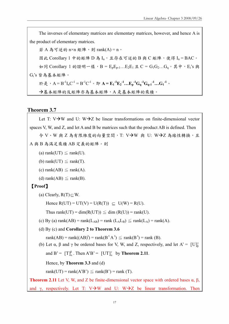
Linear Algebra- Chapter 3 20080926
17
The inverses of elementary matrices are elementary matrices however and hence A is
the product of elementary matrices
若 A 為可逆的 ntimesn 矩陣則 rank(A) = n
因此 Corollary 1 中的矩陣 D 為 In且存在可逆的 B 與 C 矩陣使得 In = BAC
如同 Corollary 1 的證明一樣B = EpEp-1hellipE2E1 且 C = G1G2hellipGq其中Eirsquos 與
Girsquos 皆為基本矩陣
於是A = B-1InC-1 = B-1C-1即 A = E1-1E2
-1hellipEp-1Gq
-1Gq-1-1hellipG1
-1
基本矩陣的反矩陣亦為基本矩陣A 是基本矩陣的乘積
Theorem 37 Let T V W and U W Z be linear transformations on finite-dimensional vector
spaces V W and Z and let A and B be matrices such that the product AB is defined Then
令 VW 與 Z 為有限維度的向量空間T V W 與 U W Z 為線性轉換且
A 與 B 為滿足乘積 AB 定義的矩陣則
(a) rank(UT) ≦ rank(U)
(b) rank(UT) ≦ rank(T)
(c) rank(AB) ≦ rank(A)
(d) rank(AB) ≦ rank(B)
【Proof】
(a) Clearly R(T)subeW
Hence R(UT) = UT(V) = U(R(T)) sube U(W) = R(U)
Thus rank(UT) = dim(R(UT)) ≦ dim (R(U)) = rank(U)
(c) By (a) rank(AB) = rank(LAB) = rank (LALB) ≦ rank(LA) = rank(A)
(d) By (c) and Corollary 2 to Theorem 36
rank(AB) = rank((AB)t) = rank(B t A t) ≦ rank(B t) = rank (B) (b) Let α β and γ be ordered bases for V W and Z respectively and let Arsquo = γ
β]U[
and Brsquo = βα]T[ Then ArsquoBrsquo = γ
α]UT[ by Theorem 211
Hence by Theorem 33 and (d)
rank(UT) = rank(ArsquoBrsquo) ≦ rank(Brsquo) = rank (T)
Theorem 211 Let V W and Z be finite-dimensional vector space with ordered bases α β
and γ respectively Let T V W and U W Z be linear transformation Then
Linear Algebra- Chapter 3 20080926
18
βα
γβ
γα = [T][U][UT] 令 VW 與 Z 是有限維度的向量空間αβ 與 γ 分別為 VW 與
Z 的有序基底令 T V W (先 α β) 且 U W Z (後 β γ)則 βα
γβ
γα = [T][U][UT]
Theorem 33 Let T V W be a linear transformation between finite dimensional vector
spaces and let β and γ be ordered bases for V and W respective Then rank(T) = rank( γ
β[T] ) 令 T V W且 β 與 γ 分別為有限維度向量空間 V 與 W 的有序基底
則 rank(T) = rank( γβ[T] )
EXAMPLE 4
(a) Let ⎟⎟⎠
⎞⎜⎜⎝
⎛minus
=11111121
A (第一列與第二列是 LI) rank(A) = 2
(b) Let ⎟⎟⎟
⎠
⎞
⎜⎜⎜
⎝
⎛=
003011011131
A (第三列與第一二列是 LD)rank(A) = 2
(c) Let ⎟⎟⎟
⎠
⎞
⎜⎜⎜
⎝
⎛
minus=
011111121321
A (三列為 LI) rank(A) = 3
The inverse of a Matrix
We have remarked that an ntimesn matrix is invertible if and only if its rank is n Since we
know how to compute the rank of any matrix we can always test a matrix to determine
whether it is invertible We now provide a simple technique for computing the inverse of a
matrix that utilizes elementary row operations
已知 ntimesn 矩陣為可逆的『若且唯若』條件為該矩陣的 Rank 等於 n
DEFINITION 34 Augmented Matrix Let A and B be mtimesn and mtimesp matrices respectively By the augmented matrix )BA(
we mean that the mtimes(n+p) matrix )BA( that is the matrix whose first n columns are the
columns of A and whose last p columns are the columns of B 設 A 與 B 分別為 mtimesn 與 mtimesp 的矩陣則增廣矩陣(Augmented matrix) )BA(
Linear Algebra- Chapter 3 20080926
19
為一 mtimes(n+p)的矩陣 )BA( 該矩陣的前 n 行(Column)為 A 的所有的行後 p
行為 B 的所有行
Let A be an invertible ntimesn matrix and consider the ntimes2n augmented matrix C= )IA( n
C= )IA( n )AI()IAAA(CA 1
nn111 minusminusminusminus ==
By Corollary 3 to Theorem 36 A-1 is the product of elementary matrices say
A = EpEp-1hellipE2E1 (A-1 是多個基本矩陣的乘積)
Thus )AI()IAAA(CA 1
nn111 minusminusminusminus == )AI(CA)IA(EEE 1
n1
n11ppminusminus
minus ==
We have the following result If A is an invertible invertible ntimesn matrix then it is
possible to transform the matrix (AIn) into the matrix (InA-1) by means of a finite
number of elementary row operations
若 A 為一可逆的 ntimesn 矩陣則可經過有限次數的基本列運算將矩陣 (AIn) 化成
(InA-1)
Conversely suppose that A is invertible and that for some ntimesn matrix B the matrix
(AIn) can be transformed into the matrix (InB) by a finite number of elementary row
operations Let E1 E2hellip Ep be the elementary matrices associated with these elementary row
operations as in Theorem 31 then
反之假設 A 是可逆且矩陣(AIn)可經有限次數的基本列運算轉換成矩陣(InB)
並令 E1 E2hellip Ep 分別為 Theorem 31 所稱的基本矩陣則
)BI()IA(EEE nn11pp =minus
Let M = EpEp-1hellipE2E1 we have 令 M = EpEp-1hellipE2E1
)BI()IA(EEE nn11pp =minus )BI()IA(M)MMA( nn ==
Linear Algebra- Chapter 3 20080926
20
Hence MA = In and M = B It follows that M = A-1 So B = A-1
可由 MA = In 及 M = B 得知M 就是 A-1故 B 就是 A-1
Thus we have the follow resultsIf A is an invertible ntimesn matrix and the matrix
(AIn) is transformed in a matrix of the form (InB) by means of a finite number of
elementary row operations then B=A-1
若 A 為一可逆的 ntimesn 矩陣且矩陣 (AIn) 可經有限次數的基本列運算化成
(InB)則 B=A-1
If on the other hand A is an ntimesn matrix that is not invertible then rank(A) lt n Hence
any attempt to transform (AIn) into a matrix of the form (InB) by means of elementary row
operations must fail
反之若 A 是一不可逆的 ntimesn 矩陣則 rank(A) lt n因此任何想利用基本列運算
要將矩陣 (AIn) 化成 (InB)的努力必定失敗
Thus we have the follow results If A is an notinvertible ntimesn matrix then any attempt
to transform (AIn) into a matrix of the form (InB) produce a row whose first n entries
are zeros
若 A 是一不可逆的 ntimesn 矩陣任何想將矩陣 (AIn) 化成 (InB)的努力最後會
產生一前 n 個元素均為 0 的列
EXAMPLE 5
We determine whether the matrix ⎟⎟⎟
⎠
⎞
⎜⎜⎜
⎝
⎛=
133242420
A is invertible and if it is we
compute its inverse
A 是否為可逆矩陣
We attempt to use elementary row operations to transfer
Linear Algebra- Chapter 3 20080926
21
⎟⎟⎟
⎠
⎞
⎜⎜⎜
⎝
⎛=
100010001
133242420
)IA( into a matrix of the form (InB)
看看能否利用基本行與列運算將矩陣 (AIn) 化成 (InB)
Interchanging rows 1 and 2
⎟⎟⎟
⎠
⎞
⎜⎜⎜
⎝
⎛
100001010
133420242
Multiplying the first row by 12
⎟⎟⎟
⎠
⎞
⎜⎜⎜
⎝
⎛
10000100
133420121 2
1
Adding -3 times row 1 to row 3
⎟⎟⎟
⎠
⎞
⎜⎜⎜
⎝
⎛
minusminusminus 1000100
230420121
23
21
Multiplying row 2 by 12 to obtain 1 in the 22 position
⎟⎟⎟
⎠
⎞
⎜⎜⎜
⎝
⎛
minus
minus
minusminus 100000
230210121
23
21
21
Adding -2 times row 2 to row 1 and 3 times row 2 to row 3
⎟⎟⎟
⎠
⎞
⎜⎜⎜
⎝
⎛
minus
minusminus
10001
400210301
23
2321
21
Multiplying row 3 by 14
⎟⎟⎟
⎠
⎞
⎜⎜⎜
⎝
⎛
minus
minusminus
41
83
8321
21
0001
100210301
Adding appropriate multiply of row 3 to row 1 and 2 completes the process
⎟⎟⎟
⎠
⎞
⎜⎜⎜
⎝
⎛
minusminus
minus
41
83
83
21
43
41
43
85
81
100010001
目標達成
Thus A is invertible and ⎟⎟⎟
⎠
⎞
⎜⎜⎜
⎝
⎛
+minus+minus+minus+minus+
=minus
41
83
83
21
43
41
43
85
81
1A
Linear Algebra- Chapter 3 20080926
22
EXAMPLE 6
We determine whether the matrix ⎟⎟⎟
⎠
⎞
⎜⎜⎜
⎝
⎛minus=451112
121A is invertible and if it is we
compute its inverse
A 是否為可逆矩陣
We attempt to use elementary row operations to transfer
⎟⎟⎟
⎠
⎞
⎜⎜⎜
⎝
⎛minus=
100010001
451112
121)IA( into a matrix of the form (InB)
看看能否利用基本行與列運算將矩陣 (AIn) 化成 (InB)
Adding -2 times row 1 to row 2 and -1 times row 1 to row 3 then addig row 2 to row
3
⎟⎟⎟
⎠
⎞
⎜⎜⎜
⎝
⎛minus
100010001
451112
121
⎟⎟⎟
⎠
⎞
⎜⎜⎜
⎝
⎛
minusminusminusminus
101012001
330330
121
⎟⎟⎟
⎠
⎞
⎜⎜⎜
⎝
⎛
minusminusminusminus
113012001
000330
121
is a matrix with row whose first 3 entries are zeros Therefore A is not invertible
最後一列前 3 個元素均為 0
EXAMPLE 7 Let T P2(R) P2(R) be defined by T(f(x)) = f(x)+frsquo(x)+frdquo(x) where frsquo(x) and frdquo(x)
denote the first and second derivatives of f(x) We use Corollary 1 to Theorem 218 to test
T for invertibility and compute the inverse if T is invertible Taking β=1 x x2 to be the
standard ordered basis of P2(R) we have
令 T P2(R) P2(R) 為線性轉換且定義為 T(f(x)) = f(x)+frsquo(x)+frdquo(x)利用
Corollary 1 to Theorem 218 來測試 T 是否可逆並計算其逆轉換取 β=1 x x2為
P2(R)的標準有序基底
T(1) = 1 = 1bull1+0bullx+0bullx2
T(x) = 1+x = 1bull1+1bullx+0bullx2
Linear Algebra- Chapter 3 20080926
23
T(x2) = 2+2x+x2 = 2bull1+2bullx+1bullx2
⎟⎟⎟
⎠
⎞
⎜⎜⎜
⎝
⎛=β
100210211
[T] 稱為 T 相對有序基底 β的座標向量
依據 Corollary 1 to Theorem 218 T 可逆『若且唯若』 β[T] 可逆且
1-1 )[T](][T minusββ =
Using the method of Examples 5 and 6 we can show that β[T] is invertible with
inverse
⎟⎟⎟
⎠
⎞
⎜⎜⎜
⎝
⎛minus
minus=minus
β
100210
011)([T] 1
Thus T is is invertible and βminusminus
β = ][T)([T] 11 Hence by Theorem 214 we have
⎟⎟⎟
⎠
⎞
⎜⎜⎜
⎝
⎛minusminus
=⎟⎟⎟
⎠
⎞
⎜⎜⎜
⎝
⎛
⎟⎟⎟
⎠
⎞
⎜⎜⎜
⎝
⎛minus
minus=++ β
minus
2
21
10
2
1
02
2101
aa2aaa
aaa
100210
011)]xaxa(a[T
Therefore T-1(a0+a1x+a2x2) = (a0-a1)+(a1-2a2)x+a2x2 Corollary 1 to Theorem 218 Let V be finite-dimensional vector space with an ordered basis β and let T V V be linear Then T is invertible if and only if β[T] is invertible
Furthermore 1-1 )[T](][T minusββ = V 為有限維度的向量空間β 是 V 的有序基底令 T
V V 為線性轉換 T 為可逆的『若且唯若』條件為 β[T] 可逆再者
1-1 )[T](][T minusββ =
Theorem 214 Let V and W be finite-dimensional vector spaces having ordered bases β and γ respectively and let T V W be linear Then for each uisinV we have β
γβγ = [u][T][T(u)]
V 與 W 為有限維度的向量空間β 與 γ分別 V 與 W 的有序基底令 T V W 為線
性轉換則 V 中的 u 映至 W 的結果 T(u) 相對於有序基底 γ 的座標向量為
βγβγ = [u][T][T(u)]
Invertible and Inverse of MATRIX Let A be an n times n matrix If a matrix B can be found such that AB = BA = In then A is
Linear Algebra- Chapter 3 20080926
24
said to be invertible and B is called the inverse of A (denote B = A-1 and A-k=(A-1)k )
If such a matrix B does not exist then A has no inverse
EXAMPLE
⎥⎦
⎤⎢⎣
⎡=
4321
A and ⎥⎦
⎤⎢⎣
⎡minus
minus=
21
23
12B
221
23
221
23
I1001
432112
BA
I100112
4321
AB
=⎥⎦
⎤⎢⎣
⎡=⎥
⎦
⎤⎢⎣
⎡⎥⎦
⎤⎢⎣
⎡minus
minus=
=⎥⎦
⎤⎢⎣
⎡=⎥
⎦
⎤⎢⎣
⎡minus
minus⎥⎦
⎤⎢⎣
⎡=
Thus AB = BA = I2 proving that the matrix A has inverse B
Theorem The inverse of an invertible matrix is unique
Let B and C be inverse of A
Thus AB = BA = In and AC = CA = In
Multiply both sides of the equation AB = In by C
C(AB) = CIn (CA)B = C
InB = C B = C
Thus an invertible matrix has only one inverse
How to find AHow to find A--11
Based on the GaussBased on the Gauss--Jordan algorithmJordan algorithmLet A be an invertible matrix Then AALet A be an invertible matrix Then AA--11=I=Inn
Let the columns of Let the columns of AA--11 be be XX11 XX22 helliphellip XXnn and the columns of I and the columns of Inn be be CC11CC22helliphellipCCnn
Find AFind A--11 by finding by finding XX11 XX22 helliphellip XXnn Write the equation AAWrite the equation AA--11=I=Inn in the formin the form
[ ] [ ]n21nn211 CCCI XXXALet LL ==minus
[ ] [ ][ ] [ ]n21n21
n21n21
CCCAXAXXACCCXXXALL
LL
=rArr=
nn2211 CAXCAX CAX === LThus
How to find AHow to find A--11
Solving these systems by using Gauss-Jordan elimination on the large augmented matrix [AC1 C2hellipCn]
Thus when A-1 exits
[ ] [ ] [ ] 1n
1nn ABwhereBIAIIA minusminus ==asympasympL
If the reduced echelon form of [If the reduced echelon form of [AIAInn] is computed and ] is computed and the first part is not of the form Ithe first part is not of the form Inn then A has no inversethen A has no inverse
[ ][ ]n21n
n21
XXXI CCCAmatrix augmented
LL
L
asympasymp
Linear Algebra- Chapter 3 20080926
25
Example Example 1212
⎥⎥⎥
⎦
⎤
⎢⎢⎢
⎣
⎡
minusminusminusminusminus
=100531010532001211
]IA[ 3
⎥⎥⎦
⎤
⎢⎢⎣
⎡minusminusminus
minusminus
+minus+
asymp
101320012110001211
1RR1R3
2)(R2
⎥⎥⎦
⎤
⎢⎢⎣
⎡minus
minusminusminusasymp
101320012110001211
R2)1(
⎥⎥⎥
⎦
⎤
⎢⎢⎢
⎣
⎡
minusminusminusminusminus
=531532211
ADetermine the inverse of
Example Example 2222
⎥⎥⎦
⎤
⎢⎢⎣
⎡
minusminusminusminus
minus++asymp
123100012110013101
R2)2(R3R2R1
⎥⎥⎦
⎤
⎢⎢⎣
⎡
minusminusminus
minus++asymp
123100135010010001
R3)1(R2R3R1
123135110
A 1
⎥⎥⎥
⎦
⎤
⎢⎢⎢
⎣
⎡
minusminusminus=minus
⎥⎥⎦
⎤
⎢⎢⎣
⎡
minusminus
minus
+minus+asymp
135000011210012301
3R2R3R2)1(R1
ExampleExampleDetermine the inverse of
⎥⎥⎦
⎤
⎢⎢⎣
⎡
minus=
412721511
A
⎥⎥⎦
⎤
⎢⎢⎣
⎡
minus=
100412010721001511
][ 3IA
⎥⎥⎦
⎤
⎢⎢⎣
⎡
minusminusminusminus
minus+minus+asymp
102630011210001511
R1)2(R31)R1(R2
There is no need to proceed further There is no need to proceed further The reduced echelon form cannot have a one in the (3 3) locatioThe reduced echelon form cannot have a one in the (3 3) location n
The reduced echelon form cannot be of the form [IThe reduced echelon form cannot be of the form [Inn B] B] Thus Thus AAndashndash11 does not existdoes not exist
Properties of Matrix InverseProperties of Matrix Inverse
Let Let AA and and BB be invertible matrices andbe invertible matrices and cc a nonzero scalar a nonzero scalar ThenThen
AA =minusminus 11)( 111 1)( 2 minusminus = A
ccA
111)( 3 minusminusminus = ABAB
nn AA )()( 4 11 minusminus =tt AA )()( 5 11 minusminus =
Color Models Color Models 1212
A color model in the context of graphics is a method of A color model in the context of graphics is a method of implementing colorsimplementing colorsThe common used models include RGB model and YIQ modelThe common used models include RGB model and YIQ modelThe RGB model is used in computer monitors and the YIQ model The RGB model is used in computer monitors and the YIQ model is used in television screensis used in television screensAn RGB computer signal can be converted to a YIQ television An RGB computer signal can be converted to a YIQ television signal using the matrix transformationsignal using the matrix transformation
⎥⎥⎥
⎦
⎤
⎢⎢⎢
⎣
⎡
⎥⎥⎥
⎦
⎤
⎢⎢⎢
⎣
⎡
minusminusminus=
⎥⎥⎥
⎦
⎤
⎢⎢⎢
⎣
⎡
BGR
311523212321275596
114587299
QIY
YIQgtRGBYIQgtRGB
Color Models Color Models 2222
A signal is converted from a television screen to a computer monA signal is converted from a television screen to a computer monitor itor using inverse of the above matrixusing inverse of the above matrix
⎥⎥⎥
⎦
⎤
⎢⎢⎢
⎣
⎡
⎥⎥⎥
⎦
⎤
⎢⎢⎢
⎣
⎡
minusminusminus=
⎥⎥⎥
⎦
⎤
⎢⎢⎢
⎣
⎡rArr
⎥⎥⎥
⎦
⎤
⎢⎢⎢
⎣
⎡
⎥⎥⎥
⎦
⎤
⎢⎢⎢
⎣
⎡
minusminusminus=
⎥⎥⎥
⎦
⎤
⎢⎢⎢
⎣
⎡minus
QIY
0751108116472721
6209561
BGR
QIY
311523212321275596
114587299
BGR 1
CryptographyCryptography 密碼學密碼學 1212
Cryptography is the process of coding and decoding messagesCryptography is the process of coding and decoding messagesThe technique can be traced back to the ancient Greeks Today The technique can be traced back to the ancient Greeks Today governments use sophisticated methods of coding and decoding governments use sophisticated methods of coding and decoding messagesmessagesOne type of code that is extremely difficult to break makes use One type of code that is extremely difficult to break makes use of a of a large matrix to encode a message large matrix to encode a message The receiver of the message decodes it using the inverse of the The receiver of the message decodes it using the inverse of the matrixmatrixThe first matrix is called the encoding matrix and its inverse The first matrix is called the encoding matrix and its inverse is is called the decoding matrixcalled the decoding matrix
Cryptography Cryptography 密碼學密碼學 2222
A A-1Message
Encoding MatrixEncoding Matrix
Decoded MessageTransmission
Decoding MatrixDecoding Matrix
Linear Algebra- Chapter 3 20080926
26
Example Example 1212
Let the message be Let the message be BUY IBM STOCKBUY IBM STOCKAnd the encoding matrix beAnd the encoding matrix be
⎥⎥⎥
⎦
⎤
⎢⎢⎢
⎣
⎡ minusminusminus
434110433
B U Y B U Y -- I B M I B M -- S T O C KS T O C K2 21 25 27 9 2 13 27 19 20 15 3 112 21 25 27 9 2 13 27 19 20 15 3 11
⎥⎥⎥
⎦
⎤
⎢⎢⎢
⎣
⎡ minusminusminusminusminus=
⎥⎥⎥
⎦
⎤
⎢⎢⎢
⎣
⎡
⎥⎥⎥
⎦
⎤
⎢⎢⎢
⎣
⎡ minusminusminus
2331372091431715418461146
222117196116169
27319225271527921112013272
434110433
EncodingEncoding
Example Example 2222
Let the message be Let the message be BUY IBM STOCKBUY IBM STOCKAnd the decoding matrix beAnd the decoding matrix be
⎥⎥⎥
⎦
⎤
⎢⎢⎢
⎣
⎡
minusminus 334344101
B U Y B U Y -- I B M I B M -- S T O C KS T O C K2 21 25 27 9 2 13 27 19 20 15 3 112 21 25 27 9 2 13 27 19 20 15 3 11
⎥⎥⎥
⎦
⎤
⎢⎢⎢
⎣
⎡=
⎥⎥⎥
⎦
⎤
⎢⎢⎢
⎣
⎡ minusminusminusminusminus
⎥⎥⎥
⎦
⎤
⎢⎢⎢
⎣
⎡
minusminus 27319225271527921112013272
2331372091431715418461146
222117196116169
334344101
DecodingDecoding
3-3 Systems of Linear Equations ndash Theoretical Aspects
The system of equations
mnmn22m11m
2nn2222121
1nn1212111
bxaxaxa
bxaxaxabxaxaxa
=+++
=+++=+++
(S)
were aij and bi (1≦i≦m and 1≦j≦n) are scalars in a field F and x1 x2hellipxn are n
variables taking values in F is called a system of m linear equations in n unknows over the
field F
上式稱為佈於 Field F 含有 n 個未知數m 個線性方程式的系統或方程組(system
of m linear equations in n unknows)
The mtimesn matrix
⎟⎟⎟⎟⎟
⎠
⎞
⎜⎜⎜⎜⎜
⎝
⎛
=
mn2m1m
n22221
n11211
aaa
aaaaaa
A is called the coefficient matrix of the
system (S)(係數矩陣) If we let
⎟⎟⎟⎟⎟
⎠
⎞
⎜⎜⎜⎜⎜
⎝
⎛
=
n
2
1
x
xx
x and
⎟⎟⎟⎟⎟
⎠
⎞
⎜⎜⎜⎜⎜
⎝
⎛
=
m
2
1
b
bb
b Then the system (S) may
be rewritten as a single matrix equation Ax = b(單一矩陣方程式)
To exploit the results that we have developed we often consider a system of linear
equations as a single matrix equation
Linear Algebra- Chapter 3 20080926
27
A solution to the system (S) is an n-tuple n
n
2
1
F
s
ss
s isin
⎟⎟⎟⎟⎟
⎠
⎞
⎜⎜⎜⎜⎜
⎝
⎛
= such that As = b The set of
all solutions to the system (S) is called the solution set of the system(解集合) System (S)
is called consistent(相容) if its solution set is nonempty otherwise it is called
inconsistent(不相容)
方程組(S)的解為一 n 序組該序組可以使 As = b方程組的所有解所成的集合
稱為該方程組的解集合(Solution set)方程組的解集合非空集合者稱為「相容」解
集合空集合者稱為「不相容」
EXAMPLE 1
Consider 6x2xx1xx3x2
321
321
=+minus=++
that is ⎟⎟⎠
⎞⎜⎜⎝
⎛=
⎟⎟⎟
⎠
⎞
⎜⎜⎜
⎝
⎛
⎟⎟⎠
⎞⎜⎜⎝
⎛minus 6
1
xxx
211132
3
2
1
(以矩陣表示)
This system has many solutions such as ⎟⎟⎟
⎠
⎞
⎜⎜⎜
⎝
⎛minus=
726
s and ⎟⎟⎟
⎠
⎞
⎜⎜⎜
⎝
⎛
minusminus=
34
8s
Consider 1xx0xx
21
21
=+=+
that is ⎟⎟⎠
⎞⎜⎜⎝
⎛=⎟⎟
⎠
⎞⎜⎜⎝
⎛⎥⎦
⎤⎢⎣
⎡10
xx
1111
2
1
顯然地方程組無解
We begin our study of system of linear equations by examining the class of
homogeneous system of linear equations 先討論齊次方程組
DEFINITION 35 Homogeneous amp Nonhomogeneous
A system Ax=b of m linear equations in n unknowns is said to be homogeneous if b=0
Otherwise the system is said to be nonhomogeneous
方程組 Ax = bb = 0 稱為齊次方程組否則稱為非齊次方程組
Any homogeneous system has at least one solution namely the zero vector The next
result gives further information about the set of solutions to a homogeneous system
Linear Algebra- Chapter 3 20080926
28
齊次方程組至少有一個解那就是『零向量』
Theorem 38 Let Ax = 0 be a homogeneous system of m linear equations in n unknowns over a field
F Let K denote the set of all solutions to Ax = 0 Then K = N(LA) hence K is a subspace
of Fn of dimension n - rank(LA) = n- rank(A)
令 Ax = 0 代表一佈於 Field 含有 n 個未知數m 個線性方程式的方程組若令
K 代表該方程組的解集合(Solution set)則 K = N(LA)K 為 Fn 內的子空間且其維
度為 n ndash rank (LA) = n - rank(A)
【Proof】
Clearly K = sisinFn As = 0 = N(LA) The second part now follows from the
dimension theorem
Nullity(T)+rank(T) = dim(V)
Nullity (LA) = dim (Fn) ndashrank (LA ) = n ndash rank (A)
DEFINTION 27 Let V and W be vector space and let T V W be linear We define
the null space (or kernel) N(T) of T to be the set of all vectors x in V such that T(x) = 0
that is N(T) = xisinV T(x) = 0 V 與 W 為向量空間且 T V W 為線性轉換定義
線性轉換 T 的 Null space 為 V 內所有滿足 T(x) = 0 的向量 x 所形成的集合註記為
N(T)Null space 的元素 x 經線性轉換 T 轉換後所對應的「像」為 0意即 T(x) = 0
Null space 內的元素的「像」皆為 0
DEFINITION 217 Let A be an mtimesn matrix with entries from a field F We denote by LA
the mapping LA Fn Fm defined by LA(x) = Ax (the matrix product A and x) for each
column vector xisinFn We call LA a left-multiplication transformation 令 A 是 mtimesn
的矩陣所有元素均來自 FLA 為 Fn 映至 Fm的線性轉換並定義為 LA(x) = Ax其中
x 為行向量(Column vector)且 xisinFnLA被稱為左乘法轉換
Theorem 23 (Dimension Theorem) Let V and W be vector spaces and let T V W be
linear If V is finite-dimensional then Nullity(T) + rank(T) = dim(V) T 的核次數
(Nullity)與秩(Rank)的和等於定義域的維度 dim(V)
Corollary Let Ax = 0 be a homogeneous system of m linear equations in n unknowns over a field
Linear Algebra- Chapter 3 20080926
29
F If m lt n the system Ax = 0 has a nonzero solution
令 Ax = 0 代表一佈於 Field 含有 n 個未知數m 個線性方程式的方程組若 m
lt n則該方程組具有一非零解
【Proof】
Suppose that m lt n Then rank(A) = rank (LA)≦m Hence dim(K) = n - rank(LA) ≧
n ndash m gt 0 where K = N(LA) Since dim(K) gt 0 Kne 0 Thus there exists a nonzero
vector sisinK so s is a nonzero solution to Ax = 0
設 m lt n則 rank(A) = rank (LA) ≦ m依據 Theorem 38K = sisinFn As = 0
= N(LA) = dim(K) = n - rank(LA) ≧ n ndash m gt 0表示 dim(K) gt 0Kne 0故存在非
零向量 s使得 Ax = 0
EXAMPLE 2
Consider 0xxx
0xx2x
321
321
=minusminus=++
Let ⎟⎟⎠
⎞⎜⎜⎝
⎛minusminus
=111
121A be the coefficient matrix of this system It is clear that rank(A)
= 2 If K is the solution set of this system then dim(K) = 3-2 = 1 Thus any nonzero
solution constitutes a basis for K
若 K 是方程組的解所組成的集合(簡稱為解集合)依 Theorem 38 得知 dim(K)
= 3 - 2 = 1因此任一非零解將形成 K 的基底
For example since ⎟⎟⎟
⎠
⎞
⎜⎜⎜
⎝
⎛minus32
1 is a solution to the given system
⎪⎭
⎪⎬
⎫
⎪⎩
⎪⎨
⎧
⎟⎟⎟
⎠
⎞
⎜⎜⎜
⎝
⎛minus32
1 is a basis for
K Thus any vector in K is of the form ⎟⎟⎟
⎠
⎞
⎜⎜⎜
⎝
⎛minus=
⎟⎟⎟
⎠
⎞
⎜⎜⎜
⎝
⎛minus
t3t2
t
32
1t where tisinR
例如因⎟⎟⎟
⎠
⎞
⎜⎜⎜
⎝
⎛minus32
1是方程組的一個解故
⎪⎭
⎪⎬
⎫
⎪⎩
⎪⎨
⎧
⎟⎟⎟
⎠
⎞
⎜⎜⎜
⎝
⎛minus32
1 為 K 的基底K 內的任一向量均
具有如下形式
⎟⎟⎟
⎠
⎞
⎜⎜⎜
⎝
⎛minus=
⎟⎟⎟
⎠
⎞
⎜⎜⎜
⎝
⎛minus
t3t2
t
32
1t
Linear Algebra- Chapter 3 20080926
30
We now turn to the study of nonhomogeneous systems Our next result shows that the
solution set of a nonhomogeneous system Ax = b can be described in terms of the solution of
the homogeneous system Ax = 0 We refer to the equation Ax = 0 as the homogeneous system
corresponding to Ax = b
以下將進一步探討「非齊次方程組」非齊次方程組 Ax = b 的解集合可利用齊次方
程組 Ax = 0 的解來加以說明因此我們可將 Ax = 0 視為 Ax = b 的齊次方程組
Theorem 39 Let K be the solution set of a system of linear equations Ax = b and let KH be the
solution set of the corresponding homogeneous system Ax = 0 Then for any solution s to
Ax = b K =s + KH = s+k kisinKH
設 K 為線性方程組 Ax = b 的解集合且 KH為對應的齊次方程組的解集合則
對 Ax = b 的任一個解 s 而言K =s + KH = s+k kisinKH
【Proof】
Let s be any solution to Ax = b
We must show that K =s + KH
If wisinK then Aw = b Hence
A(w - s) = Aw ndash As = b ndash b = 0
So w - sisinKH
Thus there exists kisinKH such that w - s = k
It follows that w = s + k isin s +KH and therefore Ksube s +KH
Conversely suppose that wisins +KH then w = s + k for some kisinKH
But then Aw = A(s + k) = As + Ak = b + 0 = b so wisinK
Therefore s +KHsubeK and thus K=s +KH
令 s 為 Ax = b 的任一個解我們必須證明「K =s + KH」
若 wisinK則 Aw = b(即 w 為 Ax = b 的解)
於是 A(w - s) = Aw ndash As = b ndash b = 0
所以 w - sisinKH(即 w-s 為 Ax = 0 的解)
w - s 既然是 KH的元素表示有一元素 kisinKH使得 w - s = kw = s + k
w = s + kisins +KH
Linear Algebra- Chapter 3 20080926
31
因此 Ksube s +KH
反之假設 wisins +KH則 KH中存在一元素 k(kisinKH)使得 w = s + k
因 Aw = A(s + k) = As + Ak = b + 0 = b
故 wisinK 是 Ax = b 的解
因此s +KHsubeK
總結K=s +KH
EXAMPLE 3
Consider 4xxx7xx2x
321
321
minus=minusminus=++
The corresponding homogeneous system is the system in Example 2 It is easily
verified that ⎟⎟⎟
⎠
⎞
⎜⎜⎜
⎝
⎛=
411
s is a solution to the preceeding nonhomogeneous system So the
solution set of the system is ⎪⎭
⎪⎬
⎫
⎪⎩
⎪⎨
⎧isin
⎟⎟⎟
⎠
⎞
⎜⎜⎜
⎝
⎛minus+
⎟⎟⎟
⎠
⎞
⎜⎜⎜
⎝
⎛= Rt
32
1t
411
K by Theorem 39
⎟⎟⎟
⎠
⎞
⎜⎜⎜
⎝
⎛=
411
s 是非齊次方程組 Ax = b 的解
⎟⎟⎟
⎠
⎞
⎜⎜⎜
⎝
⎛minus32
1是齊次方程組的解
依據 Theorem 39 得知線性方程組 Ax = b 的解集合⎪⎭
⎪⎬
⎫
⎪⎩
⎪⎨
⎧isin
⎟⎟⎟
⎠
⎞
⎜⎜⎜
⎝
⎛minus+
⎟⎟⎟
⎠
⎞
⎜⎜⎜
⎝
⎛= Rt
32
1t
411
K
The following theorem will provide us with a means of computing solutions to certain
system of linear equations
Theorem 310~311 提供計算線性方程組的解的方法
Theorem 310 Let Ax = b be a system of n linear equations in n unknowns If A is invertible then the
Linear Algebra- Chapter 3 20080926
32
system has exactly one solution namely A-1b Conversely if the system has exactly one
solution then A is invertible
令 Ax = b 為含 n 個未知數n 個線性方程式的方程組若 A 為可逆則方程組
恰有一個解解為 A-1b反之若該方程組恰有一個解則 A 為可逆
【Proof】
Suppose that A is invertible
Substituting A-1b into system we have A(A-1b)=( AA-1)b = b
Thus A-1b is a solution
If s is an arbitrary solution then As = b
Multiplying both sides by A-1 gives s= A-1b
Thus the system has one and only one solution namely A-1b
假設 A 為可逆將 A-1b 代入方程組可得 A(A-1b)=( AA-1)b = b
故 A-1b 確為方程組的解
若 s 為方程組的任意解則 As = b
兩邊乘上 A-1可得 s= A-1b
因此方程組僅有唯一的解 A-1b
Conversely suppose that the system has exactly one solution s
Let KH denot the solution set for the corresponding homogeneous system Ax = 0
By Theorem 39 s = s + KH But it is so only if KH = 0 Thus N(LA) = 0 and
hence A is invertible
反之假設方程組恰有一個解 s
令 KH為相對應齊次方程組 Ax = 0 的解集合
依據 Theorem 39要能s = s + KH唯有 KH = 0
KH = 0即表示 N(LA) = 0故 A 為可逆
EXAMPLE 4 Consider the following system of three linear equations in three unknowns
1xx3x33x2x4x2
2x4x2
321
321
32
=++=++
=+
In Example 5 of Section 32 we compute the inverse of the coefficient matrix A of
this system Thus the system has exactly one solution namely
Linear Algebra- Chapter 3 20080926
33
⎟⎟⎟
⎠
⎞
⎜⎜⎜
⎝
⎛=
133242420
A⎟⎟⎟
⎠
⎞
⎜⎜⎜
⎝
⎛
+minus+minus+minus+minus+
=minus
41
83
83
21
43
41
43
85
81
1A
⎟⎟⎟
⎠
⎞
⎜⎜⎜
⎝
⎛
minus+minus
=⎟⎟⎟
⎠
⎞
⎜⎜⎜
⎝
⎛
⎟⎟⎟
⎠
⎞
⎜⎜⎜
⎝
⎛
+minus+minus+minus+minus+
==⎟⎟⎟
⎠
⎞
⎜⎜⎜
⎝
⎛minus
814587
41
83
83
21
43
41
43
85
81
1
3
2
1
132
bAxxx
Theorem 311 Let Ax = b be a system of linear equations Then the system is consistent (相容)if
and only if rank(A) = rank (A∣b) Matrix (A b) is called the augmented matrix o∣ f the
system Ax = b
令 Ax = b 為線性方程式方程組則此方程組至少有一個解的『若且唯若』條件
為 rank(A) = rank (A∣b) 矩陣(A∣b)稱為方程組 Ax = b 的增廣矩陣
【Proof】
To say that Ax = b has a solution is equivalent to saying that bisinR(LA)
In the proof of Theorem 35 we saw that R(LA ) = span(a1 a2 an) the span of the
column of A
Thus Ax = b has a solution if and only if bisinspan(a1 a2 an)
But bisinspan(a1 a2 an) if and only if span(a1 a2 an) = span(a1 a2 an b)
This last statement is equivalent to
dim (span(a1a2an)) = dim (span(a1a2an b))
So by Theorem 35 the preceeding equation reduces to rank(A) = rank (A∣b)
Ax = b 有一解相當於 bisinR(LA)即 b 屬於線性轉換 LA的 Range
在 Theorem 35 的證明中提到 R(LA ) = span(a1a2an)aj 為 A 的第 j 個行
(Column)即線性轉換 LA 的 Range 係由矩陣 A 的行(Column)所生成
因此 Ax = b 要有一個解的『若且唯若』條件為 bisinspan(a1 a2 an)
至於 bisinspan(a1 a2 an)之條件
bisinspan(a1a2an) 的『若且唯若』條件為 span(a1a2an) = span(a1a2an
b)
其條件相當於
Linear Algebra- Chapter 3 20080926
34
dim (span(a1a2an)) = dim (span(a1a2an b))
依據 Theorem 35該條件可簡化為 rank(A) = rank (A∣b)
Theorem 35 The rank of any matrix equals the maximum number of its linearly
independent columns that is the rank of a matrix is the dimension of the subspace
generated by its column任一矩陣的 Rank 等於其最大線性獨立行向量數目即矩陣的
Rank 是由矩陣的行向量生成的子空間的維度【LA Fn Fm】
EXAMPLE 5 Recall the system of equations
1xx0xx
21
21
=+=+
Since ⎟⎟⎠
⎞⎜⎜⎝
⎛=
1111
A and ⎟⎟⎠
⎞⎜⎜⎝
⎛=
111011
)bA(
rank(A) = 1 and rank (A b) = 2∣
Because the two ranks are unequal the system has no solutions
矩陣 A 與增廣矩陣(A∣b) 的 Rank 不同故方程組沒有解
EXAMPLE 6 We can use Theorem 311 to determine whether (3 3 2) is in the range of the linear
transformation T R3 R3 defined by T(a1 a2 a3) = (a1+a2+a3 a1-a2+a3 a1+a3)
利用 Theorem 311 來判斷 (3 3 2)是否在線性轉換 T 的 Range 中其中T R3
R3 定義為 T(a1 a2 a3) = (a1+a2+a3 a1-a2+a3 a1+a3)
Now (3 3 2)isinR(T) if and only if there exists a vector s = x1 x2 x3 in R3 such that
T(s)=(3 3 2) Such a vector s must be a solution to the system
2xx3xxx3xxx
31
321
321
=+=+minus=++
Since the ranks of the coefficient matrix and the augmented matrix of this system
are 2 and 3 respectively it follows that this system has no solutions Hence (3 3 2) notin
R(T)
(3 3 2)isinR(T) 的『若且唯若』的條件為存在一向量 s = x1 x2 x3isinR3 使得
T(s)=(3 3 2)
Linear Algebra- Chapter 3 20080926
35
向量 s 必須是 2xx3xxx3xxx
31
321
321
=+=+minus=++
的解
因係數矩陣⎟⎟⎟
⎠
⎞
⎜⎜⎜
⎝
⎛minus
101111111
的 Rank 為 2增廣矩陣⎟⎟⎟
⎠
⎞
⎜⎜⎜
⎝
⎛minus
233
101111111
的 Rank 為 3兩
者不相等故方程組無解(3 3 2) notin R(T)
Theorem 311 Let Ax = b be a system of linear equations Then the system is consistent
(相容)if and only if rank(A) = rank (A∣b) Matrix (A b) is called the ∣ augmented
matrix of the system Ax = b 令 Ax = b 為線性方程式方程組則此方程組至少有一個
解的『若且唯若』條件為 rank(A) = rank (A∣b) 矩陣(A∣b)稱為方程組 Ax = b 的
增廣矩陣
Application
In 1973 Wassily Leontief won the Nobel prize in economics for his work in developing
a mathematical model that can be used to describe various economic phenomena
1973 年Wassily Leontief 因研究一數學模式來描述各種經濟現象而獲頒諾貝爾經
濟獎
CLOSED MODEL
We begin by considering a simple society composed of three peoples (industries) ndash a
farmer who gows all the food a tailor who makes all the clothing and a carpenter who builds
all the housing We assume that each person sells to and buy from a central pool and that
everything produced is consumed Since no commodities either enter or leave the system this
case is referred to as the CLOSE MODEL
考慮一個單純社會的三種人生產食物的農夫製衣的裁縫師與蓋住屋的木匠
並假設採取集中聯營買賣且每一件產品皆付諸消費由於過程中沒有任何成品進入
或脫離這個系統所以稱為「封閉模式」
Each of these three individual consumes all three of the commodities produced in the
Linear Algebra- Chapter 3 20080926
36
society Suppose that the proportion of each of the commodities consumed by each person is
given in the following table
社會中每一位皆消費所生產的三種成品且每一種產品也都被三位所消費其消
費比例如下
食物 Food 衣物 Clothing 住屋 Housing
農夫 Farmer 040 020 020
裁縫師 Tailor 010 070 020
木匠 Carpenter 050 010 060
Let p1 p2 and p3 denote the incomes of the farmer tailor and carpenter respectively To
ensure that this society survives we require that the consumption of each individual equals
his or her income
令 p1p2 與 p3 分別表示農夫裁縫師與木匠的收入並為確保這個封閉社會可以
存活假設每一位的收入等於消費
Note that the farmer consumes 20 of the clothing Because the total cost of all clothing
is p2 the tailorrsquos income the amount spent by the farmer on clothing is 020 p2 Moreover the
amount spent by the farmer on food clothing and housing must equal the farmerrsquos income
and so we obtain the equation 040 p1 + 020 p2 + 030 p3 = p1
對農夫而言農夫的衣物消費佔 20然因所有衣物的消費總額 p2 等於裁縫師的
收入所以農夫在衣物上的消費為 020 p2且農夫在食物衣物與住屋的總消費要等
於農夫的收入 p1所以農夫的收入與消費關係式
040 p1 + 020 p2 + 020 p3 = p1
Similary equations describing the expenditures of the tailor and carpenter produce the
following system of linear equations
同理分別對裁縫師與木匠進行討論可獲得下列方程組
Linear Algebra- Chapter 3 20080926
37
040 p1 + 020 p2 + 020 p3 = p1
010 p1 + 070 p2 + 020 p3 = p2
050 p1 + 010 p2 + 060 p3 = p3
This system can be written as Ap = p
其中⎟⎟⎟
⎠
⎞
⎜⎜⎜
⎝
⎛=
3
2
1
ppp
p 且⎟⎟⎟
⎠
⎞
⎜⎜⎜
⎝
⎛=
600100500200700100200200400
A 稱為輸入-輸出(或消費)矩陣
(Input-output (or consumption) matrix)
Ap = p 稱為均衡條件(Equilibrium condition)
能否利用不等式 p ≦ p 來替代等式
At first it may seem reasonable to replace the equilibrium condition by the inequality
Ap ≦ p that is the requirement that consumption not exceed production But in fact Ap ≦ p implies that Ap = p in the closed model
For otherwise there exists a k for which
sumgt
jjkjk pAp
Hence since the columns of A sum to 1
sumsumsumsum ==gt
jj
i jjij
ii ppAp which is a contradiction (出現矛盾)
答案是在封閉系統中Ap ≦ p Ap = p
One solution to the homogeneous system (I ndash A) x = 0 which is equivalent to the
equilibrium condition is ⎟⎟⎟
⎠
⎞
⎜⎜⎜
⎝
⎛=
400350250
p
Linear Algebra- Chapter 3 20080926
38
齊次方程組(I ndash A) x = 0 或均衡條件的一個解為 ⎟⎟⎟
⎠
⎞
⎜⎜⎜
⎝
⎛=
400350250
p
We may interpret this to mean that the society survives if the farmer taior and carpenter
have incomes in the proportions 253540
⎟⎟⎟
⎠
⎞
⎜⎜⎜
⎝
⎛=
400350250
p 可以解釋為若農夫裁縫師與木匠收入比例為 253540則社會將
能生存下去
Theorem 312
Let A be an ntimesn input-output matrix having the form ⎟⎟⎠
⎞⎜⎜⎝
⎛=
EDCB
A where D is a 1times(n-
1) positive vector and C is an (n-1)times1 positive vector Then (I-A)x = 0 has a one-
dimensional solution set that is generated by a nonnegative vector
設 A 為 ntimesn 輸入-輸出矩陣 ⎟⎟⎠
⎞⎜⎜⎝
⎛=
EDCB
A 其中D 為 1times(n-1)正向量C 為
(n-1)times1 正向量則(I-A)x = 0 具有一維解集合且該解集合係由一非負向量所生成
Any input-output matrix with all positive entries satisfies the hypothesis of this theorem
任何輸入-輸出矩陣滿足 Theorem 312 的基本假設條件例如
⎟⎟⎟
⎠
⎞
⎜⎜⎜
⎝
⎛=
02502503502500650500750
A
OPEN MODEL
In the OPEN MODEL we assume that there is an outside demand for each of the
commodities produced Returning to our simple society let x1 x2 and x3 be the monetary
values of food clothing and housing produced with respective outside demands d1 d2 and d3
Let A be the 3times3 matrix such that Aij represents the amount of commodity i required to
Linear Algebra- Chapter 3 20080926
39
produce one monetary unit of commodity j Then the value of the surplus of food in the
society is x1 ndash (A11x1+A12x2+A13x3) that is the value of food produced minus the value of
food consumed while producing the three commodities The assumption that everything
produced is consumed gives us a similar equilibrium condition for the open model namely
that the surplus of each of the three commodities must equal the corresponding outside
demands Hence i
3
1jjiji dxAx =minussum
=
for j=1 2 3
在「開放模式」中我們假設每一產品皆有外來的需求在前述的單純社會裡
令 x1x2 與 x3 分別代表食物衣物與住屋的貨幣價值d1d2 與 d3 為食物衣物與住
屋的外來需求價值令 A 為 3times3 矩陣Aij 表示生產『一個貨幣單位』的產品 j 所需要
的產品 i 的價值於是此社會中食物的盈餘價值為 x1 ndash (A11x1+A12x2+A13x3)即食物的
價值減去生產食物衣物與住屋所需消耗的食物的價值意即生產出來的食物價值扣
掉用去生產食物衣物與住屋所消耗掉的價值)(A11A12A13 為生產一個貨幣單位
的食物 1衣物 2 與住屋 3 所需消耗的食物 1 數量A12x2 表示生產貨幣價值為 x2的衣物
所需要的食物價值)對每一種產品而言其盈餘價值等於外來的需求價值於是
i
3
1jjiji dxAx =minussum
=
for j=123
Suppose that 30 cents worth of food 10 cents worth of clothing and 30 cents worth of
housing are required for the production of $1 worth of food Similar suppose that 20 cents
worth of food 40 cents worth of clothing and 20 cents worth of housing are required for the
production of $1 worth of clothing Finally suppose that 30 cents worth of food 10 cents
worth of clothing and 30 cents worth of housing are required for the production of $1 worth
of housing Then the input-output matrix is
⎟⎟⎟
⎠
⎞
⎜⎜⎜
⎝
⎛=
300200300100400100300200300
A
假設生產價值 1 元的食物需要價值 30 分的食物(A11 = 03)價值 10 分的衣物
(A21 = 01)及價值 30 分的住屋(A31 = 03)生產價值 1 元的衣物需要價值 20 分的
食物(A12 = 02)價值 40 分的衣物(A22 = 04)及價值 20 分的住屋(A32 = 02)生
Linear Algebra- Chapter 3 20080926
40
產價值 1 元的住屋需要價值 30 分的食物(A13 = 03)價值 10 分的衣物(A23 = 01)
及價值 30 分的住屋(A33 = 03)於是輸入輸出矩陣 A 為
⎟⎟⎟
⎠
⎞
⎜⎜⎜
⎝
⎛=
300200300100400100300200300
A
若食物的外來需求值為 300 億元衣物為 200 億元住屋值為 1 百億元則
⎟⎟⎟
⎠
⎞
⎜⎜⎜
⎝
⎛=
⎟⎟⎟
⎠
⎞
⎜⎜⎜
⎝
⎛
⎟⎟⎟
⎠
⎞
⎜⎜⎜
⎝
⎛
minusminusminusminusminusminus
=minus=
minus
minus
700600900
100200300
700200300100600100300200300
d)AI(x
1
1
⎟⎟⎟
⎠
⎞
⎜⎜⎜
⎝
⎛=
700600900
x 表示要滿足外來需求必須生產的食物價值為 900 億元衣物價值為
600 億元住屋價值為 700 億元
Theorem
Let AX = Y be a system of n linear equations in n variables If Andash1 exists the
solution is unique and is given by X = Andash1Y
【Proof】
Substitute X = Andash1Y into the matrix equation
AX = A(Andash1Y) = (AAndash1)Y = InY = Y
The solution is unique
Let X1 be any solution thus AX1 = Y Multiplying both sides of this equation by Andash1
gives
Andash1AX1= Andash1Y InX1 = Andash1Y X1 = Andash1Y
Linear Algebra- Chapter 3 20080926
41
Example Example 1212
2x5x3x3x5x3x21x2x x
321
321
321
minus=++minus=minusminus=minusminus
⎥⎥⎥
⎦
⎤
⎢⎢⎢
⎣
⎡
minus=
⎥⎥⎥
⎦
⎤
⎢⎢⎢
⎣
⎡
⎥⎥⎥
⎦
⎤
⎢⎢⎢
⎣
⎡
minusminusminusminusminus
231
xxx
531532211
3
2
1
Solve the system of equations
This system can be written in the following matrix form
⎥⎥⎥
⎦
⎤
⎢⎢⎢
⎣
⎡
minus⎥⎥⎥
⎦
⎤
⎢⎢⎢
⎣
⎡
minusminusminusminusminus
=
⎥⎥⎥
⎦
⎤
⎢⎢⎢
⎣
⎡minus
231
531532211
xxx 1
3
2
1
If the matrix of coefficients is invertible the unique solutionIf the matrix of coefficients is invertible the unique solution isis
Example Example 2222
1 2 1 issolution unique The 321 =minus== xxx
⎥⎥⎥
⎦
⎤
⎢⎢⎢
⎣
⎡minus=
⎥⎥⎥
⎦
⎤
⎢⎢⎢
⎣
⎡
minus⎥⎥⎥
⎦
⎤
⎢⎢⎢
⎣
⎡
minusminusminus=
⎥⎥⎥
⎦
⎤
⎢⎢⎢
⎣
⎡
121
231
123135110
xxx
3
2
1
⎥⎥⎥
⎦
⎤
⎢⎢⎢
⎣
⎡
minusminusminus=
⎥⎥⎥
⎦
⎤
⎢⎢⎢
⎣
⎡
minusminusminusminusminus
=
minus
minus
123135110
531532211
A
1
1
The The LeontiefLeontief IO Model in IO Model in Economics Economics 1515
The Leontief input-output model is used to analyze the interdependence of economics Wassily Leontief received a Nobel Prize in 1973 for his work in thie fieldThe practical applications of this model have proliferated until it has now become a standard tool for investigating economic structures ranging from cities and corporation to states and countriesConsider an economics situation that involves ninterdependent industries The output of any one industry is needed as input by other industries and even possibly by the industry itself
The The LeontiefLeontief IO Model in IO Model in Economics Economics 2525
How a mathematical model involving a system of linear equations can be constructed to analyze such a situationAssume that each industry produces one commodity Let aij denote the amount of input of a certain commodity i to produce unit output of commodity j In our model let the amounts of input and output be measured in dollars Thus for example a34 = 045 means that 45 centsrsquo worth of commodity 3 is required to produce one dollarrsquos worth of commodity 4
The The LeontiefLeontief IO Model in IO Model in Economics Economics 3535
aij = amount of commodity i in one dollar of commodity jaij =生產一元價值的j產品需要耗用的i產品價值
The elements aij called input coefficients define a matrix A called the input-output matrix which describes the interdependence of the industriesExtending the model to include an open sector (all non-producing sectors) The product of industries may go not only into other producing industries but also into other non-producing sectors of the economy such as consumers and governments
The The LeontiefLeontief IO Model in IO Model in Economics Economics 4545
di = demand of the open sectors from industry ixi=total output of industry I necessary to meet demands of all n industries and the open sector
sectoropen of demand
nindustry of demand
2industry of demand
22
1industry of demand
11
industry ofoutput total
ininii
i
i dxaxaxax ++sdotsdotsdot++=
output ofportion sectoropen
output ofportion tryinterindusoutput total
DAXX +=Demand matrixDemand matrix
Output matrixOutput matrix
The The LeontiefLeontief IO Model in IO Model in Economics Economics 5555
Applying the model to the economy of a country X Applying the model to the economy of a country X represents the total output of each of the producing sectors represents the total output of each of the producing sectors of the economy and AX describes the contributions made of the economy and AX describes the contributions made by the various sectors to fulfilling the intersectional input by the various sectors to fulfilling the intersectional input requirements of the economyrequirements of the economyD is equal to (XD is equal to (X--AX) the difference between total output AX) the difference between total output X and industry transaction AXX and industry transaction AXD is thus the gross national product of the economyD is thus the gross national product of the economy
Example Example 1414
Consider an economy consisting of three industries having Consider an economy consisting of three industries having the following inputthe following input--output matrix output matrix AA Determine the output Determine the output levels required of the industries to meet the demands of levels required of the industries to meet the demands of the other industries and of the open sector in each casethe other industries and of the open sector in each case
in turn 321812
and 896
1612
9
5100
021
21
103
51
51
⎥⎥⎦
⎤
⎢⎢⎣
⎡
⎥⎥⎦
⎤
⎢⎢⎣
⎡
⎥⎥⎦
⎤
⎢⎢⎣
⎡=
⎥⎥⎥
⎦
⎤
⎢⎢⎢
⎣
⎡
= DA
The unit of The unit of DD are millions of dollarsare millions of dollars
Linear Algebra- Chapter 3 20080926
42
Example Example 2424
We wish to compute the output levels X that correspond to We wish to compute the output levels X that correspond to the various open sector demands D X is given by the the various open sector demands D X is given by the equation X = AX + D Rewritten as followsequation X = AX + D Rewritten as follows
X ndash AX = D rArr (I ndash A)X = D rArr X = (I ndash A) ndash1 D
⎥⎥⎥
⎦
⎤
⎢⎢⎢
⎣
⎡
=⎥⎥⎥
⎦
⎤
⎢⎢⎢
⎣
⎡
minus⎥⎥⎦
⎤
⎢⎢⎣
⎡=minus minus
minusminus
5400
021
21
103
51
54
5100
021
21
103
51
31
100010001
get We AI
⎥⎥⎥
⎦
⎤
⎢⎢⎢
⎣
⎡
=minus minus
4500
038
35
85
32
35
1)( AI
output ofingcorrespond valuesvarious
4500
038
35
85
32
35
)(
401020883957522133
32816189121269
)(
1
1
DAI
DAIX
minus
minus
minusuarruarruarruarruarruarruarr
⎥⎥⎦
⎤
⎢⎢⎣
⎡=
⎥⎥⎦
⎤
⎢⎢⎣
⎡
⎥⎥⎥
⎦
⎤
⎢⎢⎢
⎣
⎡
=minus=
Example Example 3434
By using Gauss-Jordan elimination
dollars of milliond are units The
40
15674
and 106629
209946
are 321812
and 896
1612
9
⎥⎥⎥
⎦
⎤
⎢⎢⎢
⎣
⎡
⎥⎥⎥
⎦
⎤
⎢⎢⎢
⎣
⎡
⎥⎥⎥
⎦
⎤
⎢⎢⎢
⎣
⎡
⎥⎥⎥
⎦
⎤
⎢⎢⎢
⎣
⎡
⎥⎥⎥
⎦
⎤
⎢⎢⎢
⎣
⎡
⎥⎥⎥
⎦
⎤
⎢⎢⎢
⎣
⎡
Example Example 4444
The output levels necessary to meet the demandsThe output levels necessary to meet the demands
IAAAIAI m =++++minus ))(( 2 L
mAAAIAI ++++=minus minus L21)(
Computing (IComputing (I--A) A) --11
1m
m2m2
m2
AI)AAAI(A)AAAI(I
)AAAI)(AI(
+minus=++++minus++++=
++++minusLL
L
NOTE 0A 1m rarr+
Population Movement Population Movement 1313
In 2000 58 million of people live in cities and 142 million of In 2000 58 million of people live in cities and 142 million of people people live in the surrounding suburbs Represent this information by tlive in the surrounding suburbs Represent this information by the he matrix matrix
The probability of a person staying in the city was 096 Thus tThe probability of a person staying in the city was 096 Thus the he probability of moving to the suburbs was 004 probability of moving to the suburbs was 004 The probability of a person moving to the city was 001 the The probability of a person moving to the city was 001 the probability of remaining in suburbia was 099probability of remaining in suburbia was 099
suburbcity
990040010960
suburbcity (to))from(
⎥⎦
⎤⎢⎣
⎡=P
⎥⎦
⎤⎢⎣
⎡=
14258
X0
City population in 2001 = people who remained from 2000 + peopleCity population in 2001 = people who remained from 2000 + peoplewho moved in from the suburbs = ( 096 who moved in from the suburbs = ( 096 timestimes 58 ) + (001 58 ) + (001 timestimes 142 ) = 142 ) = 571 million571 millionSuburban population in 2001 = people who moved in from the city Suburban population in 2001 = people who moved in from the city + people who stayed from 2000 = ( 004 + people who stayed from 2000 = ( 004 timestimes 58 ) + (099 58 ) + (099 timestimes 142 ) = 142 ) = 1429 million1429 millionCan arrive at these numbers using matrix multiplicationCan arrive at these numbers using matrix multiplication
⎥⎦
⎤⎢⎣
⎡=⎥
⎦
⎤⎢⎣
⎡⎥⎦
⎤⎢⎣
⎡==
9142157
14258
990040010960
PXX 01
Population Movement Population Movement 2323
Population Movement Population Movement 3333
Assume that the population flow represented by the matrix P is unchanged over the years The population distribution X2 after 2 years is given by X2 = P X1 = P2 X0 In general
Pn is called the n-step transition matrix The (ij)th element of Pngives the probability of going from state j to state i in n stepsFor example
in
ni XPX =+
suburbcity
960150040850
P
suburbcity (to))from(
4
⎥⎦
⎤⎢⎣
⎡=
The probability of living in the city in The probability of living in the city in 2000 and being in the suburbs 4 years 2000 and being in the suburbs 4 years later is 015later is 015
Markov ChainsMarkov Chains
The probabilities in the above model depend only on the The probabilities in the above model depend only on the current state of a person whether the person is living in the current state of a person whether the person is living in the city or in suburbiacity or in suburbiaThis type of model in which the probability of going from This type of model in which the probability of going from one state to another depends only on the current state one state to another depends only on the current state rather than on a more complete historical description is rather than on a more complete historical description is called a called a Markov chainMarkov chainMarkov chains are useful tools for scientists in many Markov chains are useful tools for scientists in many fields such as geneticsfields such as genetics
Linear Algebra- Chapter 3 20080926
43
GeneticsGenetics 1414
Genetics is the branch of biology that deals with Genetics is the branch of biology that deals with heredity heredity (遺傳)(遺傳) It is the study of units called It is the study of units called genes which determine the characteristics living genes which determine the characteristics living things inherit from their parents The inheritance things inherit from their parents The inheritance (遺傳)(遺傳)of such traitsof such traits(特徵)(特徵)as sex height eye as sex height eye color and hair color of human beings and such color and hair color of human beings and such traits as petaltraits as petal(花瓣)(花瓣) color and leaf shape of color and leaf shape of plants are governed by genesplants are governed by genesIn medicine agricultureIn medicine agriculturehelliphellip
GeneticsGenetics 2424
The traits of guinea pigsThe traits of guinea pigs(天竺鼠)(天竺鼠)are long hair and short hairare long hair and short hairThe length of hair is governed by a pair of gene which we denoteThe length of hair is governed by a pair of gene which we denote A A and aand aA guinea pig may have any one of the combination of AA A guinea pig may have any one of the combination of AA AaAa or or aaaa Each of these classes is called a genotypeEach of these classes is called a genotype(基因型)(基因型)The AA type guinea pig is indistinguishable in appearance from tThe AA type guinea pig is indistinguishable in appearance from the he AaAa type type ndashndash both have long hair both have long hair ndashndash whereas the whereas the aaaa type has short hairtype has short hairThe A gene is said to dominate the a geneThe A gene is said to dominate the a geneAn animal is called dominant An animal is called dominant (顯性)(顯性)if it has AA genes hybridif it has AA genes hybrid(混種)(混種) with with AaAa genes and recessive genes and recessive (隱性)(隱性)with with aaaa genesgenes
GeneticsGenetics 3434
When two guinea pigs are crossed the offspring inherits one genWhen two guinea pigs are crossed the offspring inherits one gene e from each parent in random mannerfrom each parent in random mannerGiven the genotype of the parents we can determine the Given the genotype of the parents we can determine the probabilities of the genotype of the offspringprobabilities of the genotype of the offspring
AA+AA AA+AA probabilities of AA probabilities of AA AaAa and and aaaa are 10and 0are 10and 0Aa+AAAa+AA probabilities of AA probabilities of AA AaAa and and aaaa are are frac12frac12 frac12frac12 and 0 and 0aa+AAaa+AA probabilities of AA probabilities of AA AaAa and and aaaa are 0 1 and 0are 0 1 and 0
This series of experiments is a Markov chain having transition This series of experiments is a Markov chain having transition matrixmatrix
aaAaAA
00012100211
P
aaAaAA
⎥⎥⎥
⎦
⎤
⎢⎢⎢
⎣
⎡=
GeneticsGenetics 4444
Assume an initial population of guinea pigs made up of an Assume an initial population of guinea pigs made up of an equal number of each genotypeequal number of each genotype
⎥⎥⎥
⎦
⎤
⎢⎢⎢
⎣
⎡=
313131
X0
The fractions of following generations are
⎥⎥⎥
⎦
⎤
⎢⎢⎢
⎣
⎡=
⎥⎥⎥
⎦
⎤
⎢⎢⎢
⎣
⎡=
⎥⎥⎥
⎦
⎤
⎢⎢⎢
⎣
⎡=
⎥⎥⎥
⎦
⎤
⎢⎢⎢
⎣
⎡=
01611615
X08187
X04143
X02121
X 4321
AAAAAaAaaaaa
3-4 Systems of Linear Equations ndash Computational Aspects
DEFINITION 36 Equivalent
Two systems of linear equations are called equivalent if they have the same solution
set
兩個線性方程組稱為等價意指兩者具有相同的解集合
Elementary Transformations Transformation called elementary transformations can be used to change a system of
linear equations into another system of linear equations that have the same solution
These transformations are used to solve system of linear equations by eliminating
variables
The equivalent transformations used in terms of matrix are called ELEMENTARY
ROW OPERATION
Linear Algebra- Chapter 3 20080926
44
Equivalent System Systems of equations that are related through elementary transformations are called
equivalent systems
Matrices that are related through elementary row operations are called row equivalent
matrices
The symbol asymp is used to indicate equivalence in both cases
Theorem 313 Let Ax = b be a system of m linear equations in n unknowns and let C be an invertible
mtimesm matrix Then the system (CA)x = Cb is equivalent to Ax = b
設 Ax = b 為含 n 個未知數m 個線性方程式的方程組若 C 為可逆的mtimesm
矩陣則(CA)x = Cb 等價於 Ax = b
【Proof】
Let K be the solution set for Ax = b and Krsquo the solution set for (CA)x = Cb If wisinK
then Aw = b So (CA)w = Cb and hence wisinKrsquo Thus KsubeKrsquo
Conversely if wisinKrsquo then (CA)w = Cb Hence Aw = C-1(CA)w = C-1(Cb) = b so
wisinK Thus KrsquosubeK and therefore K=Krsquo
設 K 為 Ax = b 的解集合且 Krsquo為(CA)x = Cb 的解集合
若 wisinK則 Aw = b (CA)w = Cb故 wisinKrsquo於是 KsubeKrsquo
反之若 wisinKrsquo則(CA)w = Cb Aw = C-1(CA)w = C-1(Cb) = b故 wisinK於是
KrsquosubeK因此K=Krsquo
Corollary Let Ax = b be a system of m linear equations in n unknowns If (Arsquo brsquo) is obtained ∣
from from (A b) by a finite number of elementary row operations then the system Arsquox = ∣
brsquo is equivalent to the original system
設 Ax = b 為含 n 個未知數m 個線性方程式的方程組若(Arsquo brsquo) ∣ 是由(A b) ∣
經過有限次數的基本列運算而得則 Arsquox = brsquo 等價於 Ax = b即兩者具有相同的解
集合
【Proof】
Suppose that (Arsquo brsquo) is obtained from (A b) by elementary row operations These ∣ ∣
Linear Algebra- Chapter 3 20080926
45
may be executed by multiplying (A b) by elementary mtimesm matrices E∣ 1 E2hellipEp Let
C=EphellipE2E1 then (Arsquo brsquo) = C(A b) = (CA Cb)∣ ∣ ∣
Since each Ei is invertible so is C Now Arsquo = CA and brsquo = Cb Thus by Theorem 313
the system Arsquox = brsquo is equivalent to the system Ax = b
設(Arsquo brsquo)∣ 是由(A b)∣ 經過基本列運算取得即以基本 mtimesm 矩陣 E1 E2hellipEp
乘上 (A b)∣ (Arsquo brsquo) = C(A b) = (CA Cb∣ ∣ ∣ )其中C=EphellipE2E1
因 Ei 可逆故 C 亦為可逆 Arsquo = CA 且 brsquo = Cb
依據 Theorem 313Arsquox = brsquo 等價於 Ax = b
Theorem 313 Let Ax = b be a system of m linear equations in n unknowns and let C be an
invertible mtimesm matrix Then the system (CA)x = Cb is equivalent to Ax = b 設 Ax = b
為含 n 個未知數m 個線性方程式的方程組若 C 為可逆的mtimesm 矩陣則(CA)x
= Cb 等價於 Ax = b
We now describe a method for solving any stystem of linear equations Consider for
example the system of linear equations
探討解線性方程組的方法hellip
2xxx2x3xxx1x2x3x2x3
4321
321
4321
=minus++=++=minus++
First we form the augmented matrix ⎟⎟⎟
⎠
⎞
⎜⎜⎜
⎝
⎛
minus
minus
231
112101112323
(增廣矩陣)
Interchanging the first and third rows ⎟⎟⎟
⎠
⎞
⎜⎜⎜
⎝
⎛
minus
minus
132
132301111121
(第 13 列互調)
Adding -1 times the first row to the second row and then add -3 times the first row to
the third row ⎟⎟⎟
⎠
⎞
⎜⎜⎜
⎝
⎛
minusminusminus
minus
512
104010101121
(第 1 列乘上 -1 加到第 2 列再以 -3 乘上
第 1 列加到第 3 列)
Linear Algebra- Chapter 3 20080926
46
Multiplying the second row by -1 ⎟⎟⎟
⎠
⎞
⎜⎜⎜
⎝
⎛
minusminus
minusminusminus
51
2
104010101121
(第 2 列乘上 -1)
Adding four times the second row to the third row ⎟⎟⎟
⎠
⎞
⎜⎜⎜
⎝
⎛
minusminus
minusminusminus
91
2
300010101121
(4 乘上第 2
列加到第 3 列)
Multiplying the third row by -13 ⎟⎟⎟
⎠
⎞
⎜⎜⎜
⎝
⎛minusminus
minus
31
2
100010101121
(第 3 列乘上 -13)
Adding the third row to the first and second rows to obtain zeros in row 1 column 4
and row 2 column 4 ⎟⎟⎟
⎠
⎞
⎜⎜⎜
⎝
⎛
325
100000100121
(將第 3 列加到第 1 列及第 2 列)
Adding -2 times the second row to the first row in order to make the first row second
column entry become zero ⎟⎟⎟
⎠
⎞
⎜⎜⎜
⎝
⎛
321
100000100101
(將第 2 列乘以 -2 再加至第 1 列)
We have now obtained the desired reduction of the augmented matrix
⎟⎟⎟
⎠
⎞
⎜⎜⎜
⎝
⎛
321
100000100101
是化簡後的增廣矩陣
This matrix corresponds to the system of linear equations
對應的線性方程組為
2x3x1xx
4
2
31
===+
By Corollary to Theorem 313 this system is equivalent to the original system But this
system is easily solved Obviously x2 = 2 and x4 = 3 Moreover x1 and x3 can be any values
Linear Algebra- Chapter 3 20080926
47
provided their sum is 1 Letting x3 = t we then have x1 = 1 ndash t Thus an arbitray solution to the
original system has the form
依據 Corollary to Theorem 313 化簡後的方程組與原方程組等值此方程組的解為
x2 = 3x4 = 3x1 + x3 = 1於是原方程組的任意解可以寫成
⎟⎟⎟⎟⎟
⎠
⎞
⎜⎜⎜⎜⎜
⎝
⎛minus
+
⎟⎟⎟⎟⎟
⎠
⎞
⎜⎜⎜⎜⎜
⎝
⎛
=
⎟⎟⎟⎟⎟
⎠
⎞
⎜⎜⎜⎜⎜
⎝
⎛ minus
0101
t
3021
3t2
t1
Observe that
⎪⎪⎭
⎪⎪⎬
⎫
⎪⎪⎩
⎪⎪⎨
⎧
⎟⎟⎟⎟⎟
⎠
⎞
⎜⎜⎜⎜⎜
⎝
⎛minus
0101
is a basis for the homogeneous system of equations
corresponding to the given system
其中
⎪⎪⎭
⎪⎪⎬
⎫
⎪⎪⎩
⎪⎪⎨
⎧
⎟⎟⎟⎟⎟
⎠
⎞
⎜⎜⎜⎜⎜
⎝
⎛minus
0101
是齊次方程組解集合的一組基底
Gauss-Jordan Elimination
Let A be an n times n matrix
1 Adjoin the identity n times n matrix In to A to form the matrix [A In]
2 Compute the reduced echelon form of [A In]
(1) If the reduced echelon form is of the type [In B] then B is the inverse of A
(2) If the reduced echelon form is not of the type [In B] in that the first n times n
submatrix is not In then A has no inverse
An n times n matrix A is invertible if and only if its reduced echelon form is In
DEFINITION 37 Reduced Row Echelon Form
A matrix is said to be in reduced row echelon form if the following three conditions
are satisfied
Linear Algebra- Chapter 3 20080926
48
一個矩陣可以被稱為簡約列梯形式必須具備有下列三條件
(a) Any row containing a nonzero entry preceeds any row in which all the entries are
zero (if any)
含有非零元素的任一列排在全含零元素的任一列前面(儘可能)
(b) The first nonzero entry in each row in the only nonzero entry in its column
各列中第一個非零元素為其所在行中唯一的非零元素
(c) The first nonzero entry in each row is 1 and it occurs in a column to thr right of the
first nonzero entry in the preceeding row
各列中第一個非零元素為 1 且它出現在前一列中第一個非零元素的右邊某一
行中
Reduced Echelon Form A matrix is in reduced echelon form if
1 Any rows consisting entirely of zeros are grouped at the bottom of the matrix
2 The first nonzero element of each other row is 1 This element is called a leading 1
3 The leading 1 of each row after the first is positioned to the right of the leading 1 of
the previous row
4 All other elements in a column that contains a leading 1 are zero
Theorem 314 Gaussian Elimination Transformation Gaussian elimination transform any matrix into its reduced row echelon form
利用 Gaussian elimination 將矩陣轉換成簡約列梯形式
We now describe a method for solving a system in which the augmented matrix is in
reduced row echelon form To illustrate this procedure we consider the system
14x8x3x2x2x28x5x2xxx6x3xxxx17x9x4xx3x2
54321
54321
54321
54321
=minus+++=minus+++=minus+++=minus+++
Linear Algebra- Chapter 3 20080926
49
for which the augmented matrix is
⎟⎟⎟⎟⎟
⎠
⎞
⎜⎜⎜⎜⎜
⎝
⎛
minusminusminusminus
1486
17
83222521113111194132
(增廣矩陣)
Applying Gaussian elimination to the augmented matrix of the system produces the
following sequence of matrices
利用 Gaussian elimination method 處理增廣矩陣
⎟⎟⎟⎟⎟
⎠
⎞
⎜⎜⎜⎜⎜
⎝
⎛
minusminusminusminus
1486
17
83222521113111194132
⎟⎟⎟⎟⎟
⎠
⎞
⎜⎜⎜⎜⎜
⎝
⎛
minusminusminusminus
148
176
83222521119413231111
⎟⎟⎟⎟⎟
⎠
⎞
⎜⎜⎜⎜⎜
⎝
⎛
minusminus
minus
0213
0000021000
1011020201
The system of linear equations corresponding to thus last matrix is
對應最後矩陣的線性方程組 2x2x
1xxx3x2x2x
54
532
531
=minus=+minus=minus+
Assign x3 = t1 x5 = t2
2t22x2x1tt1xxx
3t2t23x2x2x
254
21532
21531
+=+=+minus=+minus=
++minus=++minus=
Thus an arbitray solution s is of the form
於是任意解 s 具有下列形式
s =
⎟⎟⎟⎟⎟⎟
⎠
⎞
⎜⎜⎜⎜⎜⎜
⎝
⎛minus
+
⎟⎟⎟⎟⎟⎟
⎠
⎞
⎜⎜⎜⎜⎜⎜
⎝
⎛minus
+
⎟⎟⎟⎟⎟⎟
⎠
⎞
⎜⎜⎜⎜⎜⎜
⎝
⎛
=
⎟⎟⎟⎟⎟⎟
⎠
⎞
⎜⎜⎜⎜⎜⎜
⎝
⎛
+
+minus++minus
=
⎟⎟⎟⎟⎟⎟
⎠
⎞
⎜⎜⎜⎜⎜⎜
⎝
⎛
1201
2
t
00112
t
02013
t2t2
t1tt
3t2t2
xxxxx
21
2
2
1
21
21
5
4
3
2
1
where t1t2isinR
Linear Algebra- Chapter 3 20080926
50
Notice that
⎪⎪⎪
⎭
⎪⎪⎪
⎬
⎫
⎪⎪⎪
⎩
⎪⎪⎪
⎨
⎧
⎟⎟⎟⎟⎟⎟
⎠
⎞
⎜⎜⎜⎜⎜⎜
⎝
⎛minus
⎟⎟⎟⎟⎟⎟
⎠
⎞
⎜⎜⎜⎜⎜⎜
⎝
⎛minus
1201
2
00112
is a basis for the solution set of the corresponding
homogeneous system of equation and
⎟⎟⎟⎟⎟⎟
⎠
⎞
⎜⎜⎜⎜⎜⎜
⎝
⎛
02013
is a particular solution to the original system
⎪⎪⎪
⎭
⎪⎪⎪
⎬
⎫
⎪⎪⎪
⎩
⎪⎪⎪
⎨
⎧
⎟⎟⎟⎟⎟⎟
⎠
⎞
⎜⎜⎜⎜⎜⎜
⎝
⎛minus
⎟⎟⎟⎟⎟⎟
⎠
⎞
⎜⎜⎜⎜⎜⎜
⎝
⎛minus
1201
2
00112
是齊次方程組解集合的一組基底
⎟⎟⎟⎟⎟⎟
⎠
⎞
⎜⎜⎜⎜⎜⎜
⎝
⎛
02013
是原方程組的特別解
EXAMPLE 1
The matrix ⎟⎟⎟
⎠
⎞
⎜⎜⎜
⎝
⎛
101010011
is not in reduced row echelon form
因為第一行含有第一個非零元素在第一列但第一行尚含有其他非零元素
The matrix ⎟⎟⎟
⎠
⎞
⎜⎜⎜
⎝
⎛
110010012010
is not in reduced row echelon form
因為第一列第一個非零元素不在第一列第一個非零元素的右邊
The matrix ⎟⎟⎠
⎞⎜⎜⎝
⎛010002
is not in reduced row echelon form
因為第一列的第一個非零元素不是 1
Linear Algebra- Chapter 3 20080926
51
Reduced Echelon FormReduced Echelon Form
⎥⎥⎥
⎦
⎤
⎢⎢⎢
⎣
⎡
910030107001
⎥⎥⎥
⎦
⎤
⎢⎢⎢
⎣
⎡
100001000041
⎥⎥⎥
⎦
⎤
⎢⎢⎢
⎣
⎡
000210801
Not in Reduced Echelon Form
⎥⎥⎥
⎦
⎤
⎢⎢⎢
⎣
⎡
310000004021
⎥⎥⎥
⎦
⎤
⎢⎢⎢
⎣
⎡
100000430003021
⎥⎥⎥⎥
⎦
⎤
⎢⎢⎢⎢
⎣
⎡
0000210030108071
In Reduced Echelon Form
Use GaussUse Gauss--Jordan elimination to Jordan elimination to find reduced echelon formfind reduced echelon form 1313
Step 1 Interchange rows if necessary to bring a nonzero Step 1 Interchange rows if necessary to bring a nonzero element to the top of the first nonzero column This nonzero element to the top of the first nonzero column This nonzero element is called a pivotelement is called a pivot
⎥⎥⎦
⎤
⎢⎢⎣
⎡
minusminus
minus
1211244129333
22200
⎥⎥⎥
⎦
⎤
⎢⎢⎢
⎣
⎡
minusminus
minus
harrasymp
121124422200
129333
R2R1
Use GaussUse Gauss--Jordan elimination to Jordan elimination to find reduced echelon formfind reduced echelon form 2323
Step 2 Create a 1 in the pivot location by multiplying the Step 2 Create a 1 in the pivot location by multiplying the pivot row by 1pivotpivot row by 1pivot
Step 3 Create zero elsewhere in the pivot column by adding Step 3 Create zero elsewhere in the pivot column by adding suitable multiples of the pivot row to all other rows of the suitable multiples of the pivot row to all other rows of the matrixmatrix
⎥⎥⎥
⎦
⎤
⎢⎢⎢
⎣
⎡
minusminusminus
minus
minus+asymp
412002220043111
4)R1(R3
⎥⎥⎦
⎤
⎢⎢⎣
⎡
minusminus
minus
⎟⎠⎞
⎜⎝⎛asymp
12112442220043111
R13
1
The matrix is the reduced echelon form of the given matrixThe matrix is the reduced echelon form of the given matrix
Use GaussUse Gauss--Jordan elimination to Jordan elimination to find reduced echelon formfind reduced echelon form 3333
Step 4 Cover the pivot row and all rows above it Repeat Steps Step 4 Cover the pivot row and all rows above it Repeat Steps 1 1 and 2 for the remaining and 2 for the remaining submatrixsubmatrix Repeat Step 3 for the whole Repeat Step 3 for the whole matrix Continue until the reduced echelon form is reachedmatrix Continue until the reduced echelon form is reached
⎥⎥⎥
⎦
⎤
⎢⎢⎢
⎣
⎡
minusminus
+minus+asymp
⎥⎥⎥
⎦
⎤
⎢⎢⎢
⎣
⎡
minusminus
minus++asymp
⎥⎥⎥
⎦
⎤
⎢⎢⎢
⎣
⎡
minusminusminus
minus
⎟⎠⎞
⎜⎝⎛
asymp
⎥⎥⎥
⎦
⎤
⎢⎢⎢
⎣
⎡
minusminusminus
minus
6100050100
170011
R3R22)R3(R1
610001110052011
R2)2(R3R2R1
412001110043111
R221
412002220043111
Theorem 315 Let Ax = b be a system of r nonzero equations is in n unknown Suppose that rank(A)
= rank (A b)∣ and that (A b)∣ is in reduced row echelon form Then
設 Ax = b 為含有 n 個未知數r 個非零方程式的方程組假設 rank(A) = rank
(A b)∣ 且 (A b)∣ 為簡約列梯形式於是
(a) rank(A) = r
(b) If the general solution obtained by the procedure above is of the form s = s0 + t1u1
+ t2u2 +hellip+ tn-run-r then u1 u2hellip un-r is a basis for the solution set of the
corresponding homogeneous system and s0 is a solution to the original system 由
前述方法所得的 General solution 具有下列形式
s = s0 + t1u1 + t2u2 +hellip+ tn-run-r
其中u1 u2hellip un-r為齊次方程組 Ax = 0 的解集合的一組基底且 s0 為原方
程組的一個解)
【Proof】
Since (A b)∣ is in reduced row echelon form (A b)∣ must have r nonzero rows
Clearly these rows are linearly independent by the definition of the reduced row echelon
Linear Algebra- Chapter 3 20080926
52
form and so rank (A b)∣ = r Thus rank(A) = r
Let K be the solution set for Ax = b and let KH be the solution set for Ax = 0 Setting
t1 = t2 =hellip= tn-r = 0 we see that s = s0isinK But by Theorem 39 K = s +KH Hence
KH = - s0+K = span(u1 u2hellip un-r )
Because rank(A) = r we have dim(KH) = n-r Thus since dim(KH) = n-r and KH is
generated by a set u1 u2hellip un-r containing at most n-r vectors that is a basis for KH
由於(A b)∣ 具有簡約列梯形式因此(A b)∣ 必定具有 r 個非零列由簡約列梯形
式的定義得知 r 個非零列為線性獨立故 rank (A b)∣ = rrank(A) = r
令 K 為 Ax = b 的解集合 KH 為 Ax = 0 的解集合
假設 t1 = t2 =hellip= tn-r = 0(u1 u2hellip un-r非 KH的基底)則 s = s0isinK
依據 Theorem 39K = s +KH KH = - s0+K = span(u1 u2hellip un-r )
因 rank(A) = r所以 dim(KH) = n - r 且 KH 是由u1 u2hellip un-r 所生成
故原假設「t1 = t2 =hellip= tn-r = 0」不成立
因此 KH含有最多 n - r 個向量且這些向量為 KH的基底
Theorem 39 Let K be the solution set of a system of linear equations Ax = b and let KH be
the solution set of the corresponding homogeneous system Ax = 0 Then for any solution s
to Ax = b K =s + KH = s+k kisinKH 設 K 為線性方程組 Ax = b 的解集合且 KH
為對應的齊次方程組的解集合則對 Ax = b 的任一個解 s 而言K =s + KH = s+k
kisinKH
ExampleExampleSolve the system of equationsSolve the system of equations
7537429333
321
321
321
=minusminus=+minus=+minus
xxxxxxxxx
⎥⎥⎦
⎤
⎢⎢⎣
⎡
++asymp
000012104301
R2R3R2R1 12
431243
32
31
32
31+minus=+minus=rArr=+
=+rArr xxxx
xxxx
The general solution to the system isThe general solution to the system is
parameter) a (callednumber real is where 1243
3
2
1
rrxrxrx
=+minus=+minus=
⎥⎥⎥
⎦
⎤
⎢⎢⎢
⎣
⎡
minusminusminus
minus
minus+minus+asymp
⎥⎥⎥
⎦
⎤
⎢⎢⎢
⎣
⎡
minusminusminusminus
asymp
⎥⎥⎥
⎦
⎤
⎢⎢⎢
⎣
⎡
minusminusminusminus
242012103111
1R)3(3R1R)2(2R
715374123111
715374129333
R131
ExampleExample
Solve the system of equationsSolve the system of equations446942
1423258101242
4321
4321
4321
=minus+minusminus=+minus+minus
=minus+minus
xxxxxxxxxxxx
⎪⎪
⎩
⎪⎪
⎨
⎧
===
minus=
rArr==minus=minus
rArr
1x6xrx
2r2x
1x6x
2x2x
4
3
2
1
4
3
21
⎥⎥⎥
⎦
⎤
⎢⎢⎢
⎣
⎡ minusminusasymp
⎥⎥⎥
⎦
⎤
⎢⎢⎢
⎣
⎡minus
minusminusasymp
⎥⎥⎥
⎦
⎤
⎢⎢⎢
⎣
⎡
minusminusminusminusminusasymp
⎥⎥⎥
⎦
⎤
⎢⎢⎢
⎣
⎡
minusminusminusminusminusasymp
⎥⎥⎥
⎦
⎤
⎢⎢⎢
⎣
⎡
minusminusminusminusminus
minusminusasymp
⎥⎥⎥
⎦
⎤
⎢⎢⎢
⎣
⎡
minusminusminusminusminus
minusminus
+
minus+
+
minus+
minus+
+
110006010020021
110005110011021
14430051100
295621
2R31
144300153300295621
446942142321295621
44694214232158101242
R3R2
1)R3(R1
3R2R3
6)R2(R1
2)R1(R3
R1R2R1
21
Linear Algebra- Chapter 3 20080926
53
ExampleExampleSolve the system of equationsSolve the system of equations
432636242232
54321
54321
54321
=+minus+minusminus=++minus+=++minus+
xxxxxxxxxxxxxxx
⎥⎥⎦
⎤
⎢⎢⎣
⎡ minusasymp
⎥⎥⎦
⎤
⎢⎢⎣
⎡
minusminusminusminusminus
+
minus+
642000210000213121
431121636242213121
R1R3
2)R1(R2
⎥⎥⎦
⎤
⎢⎢⎣
⎡ minusasympharr 210000
642000213121
R3R2 ( ) ⎥⎥⎦
⎤
⎢⎢⎣
⎡ minusasymp
210000321000213121
2R21
⎥⎥⎦
⎤
⎢⎢⎣
⎡ minusminusminusasympminus+ 210000
321000750121
3)R2(R1 ⎥⎥⎦
⎤
⎢⎢⎣
⎡minus
minusasymp
minus+
+
210000101000300121
2)R3(R2
5R3R1
2x1x
3xx2x
5
4
321
=minus=
++minus=rArr
2xs and r somefor 1x sx rx
3sr2x
5
432
1
=minus===
++minus=
ExampleExample
Solve the system of Solve the system of equationsequations 122
32452232
32
321
321
321
=+minus=minus+
=+minus=+minus
xxxxxxxxxxx
⎥⎥
⎦
⎤
⎢⎢
⎣
⎡asymp
minusminusminus
minus
harr1220210063303211
R3R2
( ) ⎥⎥
⎦
⎤
⎢⎢
⎣
⎡asymp
minusminusminus
minus
1220210021103211
R231
⎥⎥
⎦
⎤
⎢⎢
⎣
⎡asympminusminusminus
minus+
+
5400210021101101
2)R2(R4
R2R1 ⎥⎥
⎦
⎤
⎢⎢
⎣
⎡asymp
minusminus
minus+
+
minus+
13000210040103001
4)R3R(R4
R3R2
1)R3(R1
( ) ⎥⎥
⎦
⎤
⎢⎢
⎣
⎡asymp
minusminus
1000210040103001
R4131
The system has no solutionThe system has no solution
⎥⎥
⎦
⎤
⎢⎢
⎣
⎡asymp
⎥⎥
⎦
⎤
⎢⎢
⎣
⎡
minusminusminus
minus
minusminusminusminus
minus+
minus+
1220633021003211
1220312145223211
1)R1(R3
2)R1(R2
0x1+0x2+0x3=1
Curve FittingCurve Fitting
A set of data points A set of data points is given and it is is given and it is necessary to find a polynomial whose graph passes through the necessary to find a polynomial whose graph passes through the points points The points are often measurements in an experiment The points are often measurements in an experiment The xThe x--coordinates are called coordinates are called base pointsbase pointsIt can be shown that if the base points are all distinct then aIt can be shown that if the base points are all distinct then a unique unique polynomial of degree n polynomial of degree n ndashndash 1 (or less)1 (or less)
can be fitted to thecan be fitted to the pointspoints
) ( ) ( ) ( 2211 nn yxyxyx K
11
2210
minusminus
minusminus ++++= n
nn
n xaxaxaay K
The coefficients can be found by substituting the points The coefficients can be found by substituting the points into the polynomial equation and then solving a system into the polynomial equation and then solving a system of linear equationsof linear equations
ExampleExample
Determine the equation of the polynomial of degree 2 whose graphpasses through the points (1 6) (2 3) (3 2)
Let the polynomial be and substituting x = 1 y = 6 x = 2 y = 3 x = 3 y = 2 we have
Solving this system for a0 a1 and a2 using Gauss-Jordan elimination
⎥⎥⎥
⎦
⎤
⎢⎢⎢
⎣
⎡minus
minus
minus+minus+asymp
220033109201
1)R2(R31)R2(R1
2210 xaxaay ++=
2a9a3a3a4a2a6aaa
210
210
210
=++=++=++
⎥⎥⎥
⎦
⎤
⎢⎢⎢
⎣
⎡
minusminus
⎥⎥⎥
⎦
⎤
⎢⎢⎢
⎣
⎡
minus+minus+asymp
482033106111
293134216111
1)R1(R31)R1(R2
( )⎥⎥⎥
⎦
⎤
⎢⎢⎢
⎣
⎡minus
⎥⎥⎥
⎦
⎤
⎢⎢⎢
⎣
⎡minus
minusasymp
minus++asymp
11006010
11001
110033109201
3)R3(R22R3R1
R321
We get a0 = 11 a1 = ndash 6 a2 = 1The parabola that passes through these points is y = 11 ndash 6x + x2
ExampleExample Traffic FlowTraffic Flow
Network analysis plays an important role in electrical Network analysis plays an important role in electrical engineeringengineeringThe concepts and tools of network analysis have been The concepts and tools of network analysis have been found to be useful in many other fields such as found to be useful in many other fields such as information theory and the study of transportation systemsinformation theory and the study of transportation systemsThe analysis of traffic flow through a road network during The analysis of traffic flow through a road network during peak period illustrates how systems of linear equations peak period illustrates how systems of linear equations with with manymany solutions can arise in practicesolutions can arise in practice
Traffic FlowTraffic Flow
Consider the typical road network The streets are all oneConsider the typical road network The streets are all one--way with the arrows indicating the direction of traffic flowway with the arrows indicating the direction of traffic flowThe flow of traffic in and out of the network is measured The flow of traffic in and out of the network is measured in vehicles per hour (in vehicles per hour (vphvph))How to construct a mathematical model to analyze this How to construct a mathematical model to analyze this network network
Traffic Traffic FlowFlowTRAFFIC LAWTRAFFIC LAWhelliphellipAll traffic entering an intersection must leave that All traffic entering an intersection must leave that intersectionintersection
Linear Algebra- Chapter 3 20080926
54
Junction AJunction BJunction CJunction DJunction EJunction F 600
800 200 500 100 600
54
643
73
72
621
51
=+=++minus=+minus=minus=+minus=+
xxxxx
xxxx
xxxxx
⎥⎥⎥⎥⎥⎥⎥⎥⎥⎥⎥⎥⎥
⎦
⎤
⎢⎢⎢⎢⎢⎢⎢⎢⎢⎢⎢⎢⎢
⎣
⎡
asympasymp
⎥⎥⎥⎥⎥⎥⎥⎥⎥⎥⎥⎥⎥
⎦
⎤
⎢⎢⎢⎢⎢⎢⎢⎢⎢⎢⎢⎢⎢
⎣
⎡
minusminus
minusminusminusminus
minusminus
minusminus
0000000001110000
6001101000200100010050010000106001100001
600001100080001011002001000100500100001010001000116000010001
L
Traffic FlowTraffic FlowJunction AJunction BJunction CJunction DJunction EJunction F 600
800 200 500 100 600
54
643
73
72
621
51
=+=++minus=+minus=minus=+minus=+
xxxxx
xxxx
xxxxx
Perform road work on x7 Because x3 ge 0 the minimum flow 200 in the branch x7 can be obtained by making x3 = 0 (closing DE to traffic)
Traffic FlowTraffic Flow
We get
765
76473
72761
xx x600xxx200x x500x x600xxx
minus=++minus=minus=+=+minusminus=
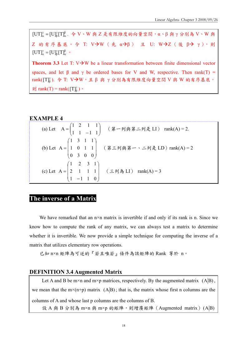
Linear Algebra- Chapter 3 20080926
20
Hence MA = In and M = B It follows that M = A-1 So B = A-1
可由 MA = In 及 M = B 得知M 就是 A-1故 B 就是 A-1
Thus we have the follow resultsIf A is an invertible ntimesn matrix and the matrix
(AIn) is transformed in a matrix of the form (InB) by means of a finite number of
elementary row operations then B=A-1
若 A 為一可逆的 ntimesn 矩陣且矩陣 (AIn) 可經有限次數的基本列運算化成
(InB)則 B=A-1
If on the other hand A is an ntimesn matrix that is not invertible then rank(A) lt n Hence
any attempt to transform (AIn) into a matrix of the form (InB) by means of elementary row
operations must fail
反之若 A 是一不可逆的 ntimesn 矩陣則 rank(A) lt n因此任何想利用基本列運算
要將矩陣 (AIn) 化成 (InB)的努力必定失敗
Thus we have the follow results If A is an notinvertible ntimesn matrix then any attempt
to transform (AIn) into a matrix of the form (InB) produce a row whose first n entries
are zeros
若 A 是一不可逆的 ntimesn 矩陣任何想將矩陣 (AIn) 化成 (InB)的努力最後會
產生一前 n 個元素均為 0 的列
EXAMPLE 5
We determine whether the matrix ⎟⎟⎟
⎠
⎞
⎜⎜⎜
⎝
⎛=
133242420
A is invertible and if it is we
compute its inverse
A 是否為可逆矩陣
We attempt to use elementary row operations to transfer
Linear Algebra- Chapter 3 20080926
21
⎟⎟⎟
⎠
⎞
⎜⎜⎜
⎝
⎛=
100010001
133242420
)IA( into a matrix of the form (InB)
看看能否利用基本行與列運算將矩陣 (AIn) 化成 (InB)
Interchanging rows 1 and 2
⎟⎟⎟
⎠
⎞
⎜⎜⎜
⎝
⎛
100001010
133420242
Multiplying the first row by 12
⎟⎟⎟
⎠
⎞
⎜⎜⎜
⎝
⎛
10000100
133420121 2
1
Adding -3 times row 1 to row 3
⎟⎟⎟
⎠
⎞
⎜⎜⎜
⎝
⎛
minusminusminus 1000100
230420121
23
21
Multiplying row 2 by 12 to obtain 1 in the 22 position
⎟⎟⎟
⎠
⎞
⎜⎜⎜
⎝
⎛
minus
minus
minusminus 100000
230210121
23
21
21
Adding -2 times row 2 to row 1 and 3 times row 2 to row 3
⎟⎟⎟
⎠
⎞
⎜⎜⎜
⎝
⎛
minus
minusminus
10001
400210301
23
2321
21
Multiplying row 3 by 14
⎟⎟⎟
⎠
⎞
⎜⎜⎜
⎝
⎛
minus
minusminus
41
83
8321
21
0001
100210301
Adding appropriate multiply of row 3 to row 1 and 2 completes the process
⎟⎟⎟
⎠
⎞
⎜⎜⎜
⎝
⎛
minusminus
minus
41
83
83
21
43
41
43
85
81
100010001
目標達成
Thus A is invertible and ⎟⎟⎟
⎠
⎞
⎜⎜⎜
⎝
⎛
+minus+minus+minus+minus+
=minus
41
83
83
21
43
41
43
85
81
1A
Linear Algebra- Chapter 3 20080926
22
EXAMPLE 6
We determine whether the matrix ⎟⎟⎟
⎠
⎞
⎜⎜⎜
⎝
⎛minus=451112
121A is invertible and if it is we
compute its inverse
A 是否為可逆矩陣
We attempt to use elementary row operations to transfer
⎟⎟⎟
⎠
⎞
⎜⎜⎜
⎝
⎛minus=
100010001
451112
121)IA( into a matrix of the form (InB)
看看能否利用基本行與列運算將矩陣 (AIn) 化成 (InB)
Adding -2 times row 1 to row 2 and -1 times row 1 to row 3 then addig row 2 to row
3
⎟⎟⎟
⎠
⎞
⎜⎜⎜
⎝
⎛minus
100010001
451112
121
⎟⎟⎟
⎠
⎞
⎜⎜⎜
⎝
⎛
minusminusminusminus
101012001
330330
121
⎟⎟⎟
⎠
⎞
⎜⎜⎜
⎝
⎛
minusminusminusminus
113012001
000330
121
is a matrix with row whose first 3 entries are zeros Therefore A is not invertible
最後一列前 3 個元素均為 0
EXAMPLE 7 Let T P2(R) P2(R) be defined by T(f(x)) = f(x)+frsquo(x)+frdquo(x) where frsquo(x) and frdquo(x)
denote the first and second derivatives of f(x) We use Corollary 1 to Theorem 218 to test
T for invertibility and compute the inverse if T is invertible Taking β=1 x x2 to be the
standard ordered basis of P2(R) we have
令 T P2(R) P2(R) 為線性轉換且定義為 T(f(x)) = f(x)+frsquo(x)+frdquo(x)利用
Corollary 1 to Theorem 218 來測試 T 是否可逆並計算其逆轉換取 β=1 x x2為
P2(R)的標準有序基底
T(1) = 1 = 1bull1+0bullx+0bullx2
T(x) = 1+x = 1bull1+1bullx+0bullx2
Linear Algebra- Chapter 3 20080926
23
T(x2) = 2+2x+x2 = 2bull1+2bullx+1bullx2
⎟⎟⎟
⎠
⎞
⎜⎜⎜
⎝
⎛=β
100210211
[T] 稱為 T 相對有序基底 β的座標向量
依據 Corollary 1 to Theorem 218 T 可逆『若且唯若』 β[T] 可逆且
1-1 )[T](][T minusββ =
Using the method of Examples 5 and 6 we can show that β[T] is invertible with
inverse
⎟⎟⎟
⎠
⎞
⎜⎜⎜
⎝
⎛minus
minus=minus
β
100210
011)([T] 1
Thus T is is invertible and βminusminus
β = ][T)([T] 11 Hence by Theorem 214 we have
⎟⎟⎟
⎠
⎞
⎜⎜⎜
⎝
⎛minusminus
=⎟⎟⎟
⎠
⎞
⎜⎜⎜
⎝
⎛
⎟⎟⎟
⎠
⎞
⎜⎜⎜
⎝
⎛minus
minus=++ β
minus
2
21
10
2
1
02
2101
aa2aaa
aaa
100210
011)]xaxa(a[T
Therefore T-1(a0+a1x+a2x2) = (a0-a1)+(a1-2a2)x+a2x2 Corollary 1 to Theorem 218 Let V be finite-dimensional vector space with an ordered basis β and let T V V be linear Then T is invertible if and only if β[T] is invertible
Furthermore 1-1 )[T](][T minusββ = V 為有限維度的向量空間β 是 V 的有序基底令 T
V V 為線性轉換 T 為可逆的『若且唯若』條件為 β[T] 可逆再者
1-1 )[T](][T minusββ =
Theorem 214 Let V and W be finite-dimensional vector spaces having ordered bases β and γ respectively and let T V W be linear Then for each uisinV we have β
γβγ = [u][T][T(u)]
V 與 W 為有限維度的向量空間β 與 γ分別 V 與 W 的有序基底令 T V W 為線
性轉換則 V 中的 u 映至 W 的結果 T(u) 相對於有序基底 γ 的座標向量為
βγβγ = [u][T][T(u)]
Invertible and Inverse of MATRIX Let A be an n times n matrix If a matrix B can be found such that AB = BA = In then A is
Linear Algebra- Chapter 3 20080926
24
said to be invertible and B is called the inverse of A (denote B = A-1 and A-k=(A-1)k )
If such a matrix B does not exist then A has no inverse
EXAMPLE
⎥⎦
⎤⎢⎣
⎡=
4321
A and ⎥⎦
⎤⎢⎣
⎡minus
minus=
21
23
12B
221
23
221
23
I1001
432112
BA
I100112
4321
AB
=⎥⎦
⎤⎢⎣
⎡=⎥
⎦
⎤⎢⎣
⎡⎥⎦
⎤⎢⎣
⎡minus
minus=
=⎥⎦
⎤⎢⎣
⎡=⎥
⎦
⎤⎢⎣
⎡minus
minus⎥⎦
⎤⎢⎣
⎡=
Thus AB = BA = I2 proving that the matrix A has inverse B
Theorem The inverse of an invertible matrix is unique
Let B and C be inverse of A
Thus AB = BA = In and AC = CA = In
Multiply both sides of the equation AB = In by C
C(AB) = CIn (CA)B = C
InB = C B = C
Thus an invertible matrix has only one inverse
How to find AHow to find A--11
Based on the GaussBased on the Gauss--Jordan algorithmJordan algorithmLet A be an invertible matrix Then AALet A be an invertible matrix Then AA--11=I=Inn
Let the columns of Let the columns of AA--11 be be XX11 XX22 helliphellip XXnn and the columns of I and the columns of Inn be be CC11CC22helliphellipCCnn
Find AFind A--11 by finding by finding XX11 XX22 helliphellip XXnn Write the equation AAWrite the equation AA--11=I=Inn in the formin the form
[ ] [ ]n21nn211 CCCI XXXALet LL ==minus
[ ] [ ][ ] [ ]n21n21
n21n21
CCCAXAXXACCCXXXALL
LL
=rArr=
nn2211 CAXCAX CAX === LThus
How to find AHow to find A--11
Solving these systems by using Gauss-Jordan elimination on the large augmented matrix [AC1 C2hellipCn]
Thus when A-1 exits
[ ] [ ] [ ] 1n
1nn ABwhereBIAIIA minusminus ==asympasympL
If the reduced echelon form of [If the reduced echelon form of [AIAInn] is computed and ] is computed and the first part is not of the form Ithe first part is not of the form Inn then A has no inversethen A has no inverse
[ ][ ]n21n
n21
XXXI CCCAmatrix augmented
LL
L
asympasymp
Linear Algebra- Chapter 3 20080926
25
Example Example 1212
⎥⎥⎥
⎦
⎤
⎢⎢⎢
⎣
⎡
minusminusminusminusminus
=100531010532001211
]IA[ 3
⎥⎥⎦
⎤
⎢⎢⎣
⎡minusminusminus
minusminus
+minus+
asymp
101320012110001211
1RR1R3
2)(R2
⎥⎥⎦
⎤
⎢⎢⎣
⎡minus
minusminusminusasymp
101320012110001211
R2)1(
⎥⎥⎥
⎦
⎤
⎢⎢⎢
⎣
⎡
minusminusminusminusminus
=531532211
ADetermine the inverse of
Example Example 2222
⎥⎥⎦
⎤
⎢⎢⎣
⎡
minusminusminusminus
minus++asymp
123100012110013101
R2)2(R3R2R1
⎥⎥⎦
⎤
⎢⎢⎣
⎡
minusminusminus
minus++asymp
123100135010010001
R3)1(R2R3R1
123135110
A 1
⎥⎥⎥
⎦
⎤
⎢⎢⎢
⎣
⎡
minusminusminus=minus
⎥⎥⎦
⎤
⎢⎢⎣
⎡
minusminus
minus
+minus+asymp
135000011210012301
3R2R3R2)1(R1
ExampleExampleDetermine the inverse of
⎥⎥⎦
⎤
⎢⎢⎣
⎡
minus=
412721511
A
⎥⎥⎦
⎤
⎢⎢⎣
⎡
minus=
100412010721001511
][ 3IA
⎥⎥⎦
⎤
⎢⎢⎣
⎡
minusminusminusminus
minus+minus+asymp
102630011210001511
R1)2(R31)R1(R2
There is no need to proceed further There is no need to proceed further The reduced echelon form cannot have a one in the (3 3) locatioThe reduced echelon form cannot have a one in the (3 3) location n
The reduced echelon form cannot be of the form [IThe reduced echelon form cannot be of the form [Inn B] B] Thus Thus AAndashndash11 does not existdoes not exist
Properties of Matrix InverseProperties of Matrix Inverse
Let Let AA and and BB be invertible matrices andbe invertible matrices and cc a nonzero scalar a nonzero scalar ThenThen
AA =minusminus 11)( 111 1)( 2 minusminus = A
ccA
111)( 3 minusminusminus = ABAB
nn AA )()( 4 11 minusminus =tt AA )()( 5 11 minusminus =
Color Models Color Models 1212
A color model in the context of graphics is a method of A color model in the context of graphics is a method of implementing colorsimplementing colorsThe common used models include RGB model and YIQ modelThe common used models include RGB model and YIQ modelThe RGB model is used in computer monitors and the YIQ model The RGB model is used in computer monitors and the YIQ model is used in television screensis used in television screensAn RGB computer signal can be converted to a YIQ television An RGB computer signal can be converted to a YIQ television signal using the matrix transformationsignal using the matrix transformation
⎥⎥⎥
⎦
⎤
⎢⎢⎢
⎣
⎡
⎥⎥⎥
⎦
⎤
⎢⎢⎢
⎣
⎡
minusminusminus=
⎥⎥⎥
⎦
⎤
⎢⎢⎢
⎣
⎡
BGR
311523212321275596
114587299
QIY
YIQgtRGBYIQgtRGB
Color Models Color Models 2222
A signal is converted from a television screen to a computer monA signal is converted from a television screen to a computer monitor itor using inverse of the above matrixusing inverse of the above matrix
⎥⎥⎥
⎦
⎤
⎢⎢⎢
⎣
⎡
⎥⎥⎥
⎦
⎤
⎢⎢⎢
⎣
⎡
minusminusminus=
⎥⎥⎥
⎦
⎤
⎢⎢⎢
⎣
⎡rArr
⎥⎥⎥
⎦
⎤
⎢⎢⎢
⎣
⎡
⎥⎥⎥
⎦
⎤
⎢⎢⎢
⎣
⎡
minusminusminus=
⎥⎥⎥
⎦
⎤
⎢⎢⎢
⎣
⎡minus
QIY
0751108116472721
6209561
BGR
QIY
311523212321275596
114587299
BGR 1
CryptographyCryptography 密碼學密碼學 1212
Cryptography is the process of coding and decoding messagesCryptography is the process of coding and decoding messagesThe technique can be traced back to the ancient Greeks Today The technique can be traced back to the ancient Greeks Today governments use sophisticated methods of coding and decoding governments use sophisticated methods of coding and decoding messagesmessagesOne type of code that is extremely difficult to break makes use One type of code that is extremely difficult to break makes use of a of a large matrix to encode a message large matrix to encode a message The receiver of the message decodes it using the inverse of the The receiver of the message decodes it using the inverse of the matrixmatrixThe first matrix is called the encoding matrix and its inverse The first matrix is called the encoding matrix and its inverse is is called the decoding matrixcalled the decoding matrix
Cryptography Cryptography 密碼學密碼學 2222
A A-1Message
Encoding MatrixEncoding Matrix
Decoded MessageTransmission
Decoding MatrixDecoding Matrix
Linear Algebra- Chapter 3 20080926
26
Example Example 1212
Let the message be Let the message be BUY IBM STOCKBUY IBM STOCKAnd the encoding matrix beAnd the encoding matrix be
⎥⎥⎥
⎦
⎤
⎢⎢⎢
⎣
⎡ minusminusminus
434110433
B U Y B U Y -- I B M I B M -- S T O C KS T O C K2 21 25 27 9 2 13 27 19 20 15 3 112 21 25 27 9 2 13 27 19 20 15 3 11
⎥⎥⎥
⎦
⎤
⎢⎢⎢
⎣
⎡ minusminusminusminusminus=
⎥⎥⎥
⎦
⎤
⎢⎢⎢
⎣
⎡
⎥⎥⎥
⎦
⎤
⎢⎢⎢
⎣
⎡ minusminusminus
2331372091431715418461146
222117196116169
27319225271527921112013272
434110433
EncodingEncoding
Example Example 2222
Let the message be Let the message be BUY IBM STOCKBUY IBM STOCKAnd the decoding matrix beAnd the decoding matrix be
⎥⎥⎥
⎦
⎤
⎢⎢⎢
⎣
⎡
minusminus 334344101
B U Y B U Y -- I B M I B M -- S T O C KS T O C K2 21 25 27 9 2 13 27 19 20 15 3 112 21 25 27 9 2 13 27 19 20 15 3 11
⎥⎥⎥
⎦
⎤
⎢⎢⎢
⎣
⎡=
⎥⎥⎥
⎦
⎤
⎢⎢⎢
⎣
⎡ minusminusminusminusminus
⎥⎥⎥
⎦
⎤
⎢⎢⎢
⎣
⎡
minusminus 27319225271527921112013272
2331372091431715418461146
222117196116169
334344101
DecodingDecoding
3-3 Systems of Linear Equations ndash Theoretical Aspects
The system of equations
mnmn22m11m
2nn2222121
1nn1212111
bxaxaxa
bxaxaxabxaxaxa
=+++
=+++=+++
(S)
were aij and bi (1≦i≦m and 1≦j≦n) are scalars in a field F and x1 x2hellipxn are n
variables taking values in F is called a system of m linear equations in n unknows over the
field F
上式稱為佈於 Field F 含有 n 個未知數m 個線性方程式的系統或方程組(system
of m linear equations in n unknows)
The mtimesn matrix
⎟⎟⎟⎟⎟
⎠
⎞
⎜⎜⎜⎜⎜
⎝
⎛
=
mn2m1m
n22221
n11211
aaa
aaaaaa
A is called the coefficient matrix of the
system (S)(係數矩陣) If we let
⎟⎟⎟⎟⎟
⎠
⎞
⎜⎜⎜⎜⎜
⎝
⎛
=
n
2
1
x
xx
x and
⎟⎟⎟⎟⎟
⎠
⎞
⎜⎜⎜⎜⎜
⎝
⎛
=
m
2
1
b
bb
b Then the system (S) may
be rewritten as a single matrix equation Ax = b(單一矩陣方程式)
To exploit the results that we have developed we often consider a system of linear
equations as a single matrix equation
Linear Algebra- Chapter 3 20080926
27
A solution to the system (S) is an n-tuple n
n
2
1
F
s
ss
s isin
⎟⎟⎟⎟⎟
⎠
⎞
⎜⎜⎜⎜⎜
⎝
⎛
= such that As = b The set of
all solutions to the system (S) is called the solution set of the system(解集合) System (S)
is called consistent(相容) if its solution set is nonempty otherwise it is called
inconsistent(不相容)
方程組(S)的解為一 n 序組該序組可以使 As = b方程組的所有解所成的集合
稱為該方程組的解集合(Solution set)方程組的解集合非空集合者稱為「相容」解
集合空集合者稱為「不相容」
EXAMPLE 1
Consider 6x2xx1xx3x2
321
321
=+minus=++
that is ⎟⎟⎠
⎞⎜⎜⎝
⎛=
⎟⎟⎟
⎠
⎞
⎜⎜⎜
⎝
⎛
⎟⎟⎠
⎞⎜⎜⎝
⎛minus 6
1
xxx
211132
3
2
1
(以矩陣表示)
This system has many solutions such as ⎟⎟⎟
⎠
⎞
⎜⎜⎜
⎝
⎛minus=
726
s and ⎟⎟⎟
⎠
⎞
⎜⎜⎜
⎝
⎛
minusminus=
34
8s
Consider 1xx0xx
21
21
=+=+
that is ⎟⎟⎠
⎞⎜⎜⎝
⎛=⎟⎟
⎠
⎞⎜⎜⎝
⎛⎥⎦
⎤⎢⎣
⎡10
xx
1111
2
1
顯然地方程組無解
We begin our study of system of linear equations by examining the class of
homogeneous system of linear equations 先討論齊次方程組
DEFINITION 35 Homogeneous amp Nonhomogeneous
A system Ax=b of m linear equations in n unknowns is said to be homogeneous if b=0
Otherwise the system is said to be nonhomogeneous
方程組 Ax = bb = 0 稱為齊次方程組否則稱為非齊次方程組
Any homogeneous system has at least one solution namely the zero vector The next
result gives further information about the set of solutions to a homogeneous system
Linear Algebra- Chapter 3 20080926
28
齊次方程組至少有一個解那就是『零向量』
Theorem 38 Let Ax = 0 be a homogeneous system of m linear equations in n unknowns over a field
F Let K denote the set of all solutions to Ax = 0 Then K = N(LA) hence K is a subspace
of Fn of dimension n - rank(LA) = n- rank(A)
令 Ax = 0 代表一佈於 Field 含有 n 個未知數m 個線性方程式的方程組若令
K 代表該方程組的解集合(Solution set)則 K = N(LA)K 為 Fn 內的子空間且其維
度為 n ndash rank (LA) = n - rank(A)
【Proof】
Clearly K = sisinFn As = 0 = N(LA) The second part now follows from the
dimension theorem
Nullity(T)+rank(T) = dim(V)
Nullity (LA) = dim (Fn) ndashrank (LA ) = n ndash rank (A)
DEFINTION 27 Let V and W be vector space and let T V W be linear We define
the null space (or kernel) N(T) of T to be the set of all vectors x in V such that T(x) = 0
that is N(T) = xisinV T(x) = 0 V 與 W 為向量空間且 T V W 為線性轉換定義
線性轉換 T 的 Null space 為 V 內所有滿足 T(x) = 0 的向量 x 所形成的集合註記為
N(T)Null space 的元素 x 經線性轉換 T 轉換後所對應的「像」為 0意即 T(x) = 0
Null space 內的元素的「像」皆為 0
DEFINITION 217 Let A be an mtimesn matrix with entries from a field F We denote by LA
the mapping LA Fn Fm defined by LA(x) = Ax (the matrix product A and x) for each
column vector xisinFn We call LA a left-multiplication transformation 令 A 是 mtimesn
的矩陣所有元素均來自 FLA 為 Fn 映至 Fm的線性轉換並定義為 LA(x) = Ax其中
x 為行向量(Column vector)且 xisinFnLA被稱為左乘法轉換
Theorem 23 (Dimension Theorem) Let V and W be vector spaces and let T V W be
linear If V is finite-dimensional then Nullity(T) + rank(T) = dim(V) T 的核次數
(Nullity)與秩(Rank)的和等於定義域的維度 dim(V)
Corollary Let Ax = 0 be a homogeneous system of m linear equations in n unknowns over a field
Linear Algebra- Chapter 3 20080926
29
F If m lt n the system Ax = 0 has a nonzero solution
令 Ax = 0 代表一佈於 Field 含有 n 個未知數m 個線性方程式的方程組若 m
lt n則該方程組具有一非零解
【Proof】
Suppose that m lt n Then rank(A) = rank (LA)≦m Hence dim(K) = n - rank(LA) ≧
n ndash m gt 0 where K = N(LA) Since dim(K) gt 0 Kne 0 Thus there exists a nonzero
vector sisinK so s is a nonzero solution to Ax = 0
設 m lt n則 rank(A) = rank (LA) ≦ m依據 Theorem 38K = sisinFn As = 0
= N(LA) = dim(K) = n - rank(LA) ≧ n ndash m gt 0表示 dim(K) gt 0Kne 0故存在非
零向量 s使得 Ax = 0
EXAMPLE 2
Consider 0xxx
0xx2x
321
321
=minusminus=++
Let ⎟⎟⎠
⎞⎜⎜⎝
⎛minusminus
=111
121A be the coefficient matrix of this system It is clear that rank(A)
= 2 If K is the solution set of this system then dim(K) = 3-2 = 1 Thus any nonzero
solution constitutes a basis for K
若 K 是方程組的解所組成的集合(簡稱為解集合)依 Theorem 38 得知 dim(K)
= 3 - 2 = 1因此任一非零解將形成 K 的基底
For example since ⎟⎟⎟
⎠
⎞
⎜⎜⎜
⎝
⎛minus32
1 is a solution to the given system
⎪⎭
⎪⎬
⎫
⎪⎩
⎪⎨
⎧
⎟⎟⎟
⎠
⎞
⎜⎜⎜
⎝
⎛minus32
1 is a basis for
K Thus any vector in K is of the form ⎟⎟⎟
⎠
⎞
⎜⎜⎜
⎝
⎛minus=
⎟⎟⎟
⎠
⎞
⎜⎜⎜
⎝
⎛minus
t3t2
t
32
1t where tisinR
例如因⎟⎟⎟
⎠
⎞
⎜⎜⎜
⎝
⎛minus32
1是方程組的一個解故
⎪⎭
⎪⎬
⎫
⎪⎩
⎪⎨
⎧
⎟⎟⎟
⎠
⎞
⎜⎜⎜
⎝
⎛minus32
1 為 K 的基底K 內的任一向量均
具有如下形式
⎟⎟⎟
⎠
⎞
⎜⎜⎜
⎝
⎛minus=
⎟⎟⎟
⎠
⎞
⎜⎜⎜
⎝
⎛minus
t3t2
t
32
1t
Linear Algebra- Chapter 3 20080926
30
We now turn to the study of nonhomogeneous systems Our next result shows that the
solution set of a nonhomogeneous system Ax = b can be described in terms of the solution of
the homogeneous system Ax = 0 We refer to the equation Ax = 0 as the homogeneous system
corresponding to Ax = b
以下將進一步探討「非齊次方程組」非齊次方程組 Ax = b 的解集合可利用齊次方
程組 Ax = 0 的解來加以說明因此我們可將 Ax = 0 視為 Ax = b 的齊次方程組
Theorem 39 Let K be the solution set of a system of linear equations Ax = b and let KH be the
solution set of the corresponding homogeneous system Ax = 0 Then for any solution s to
Ax = b K =s + KH = s+k kisinKH
設 K 為線性方程組 Ax = b 的解集合且 KH為對應的齊次方程組的解集合則
對 Ax = b 的任一個解 s 而言K =s + KH = s+k kisinKH
【Proof】
Let s be any solution to Ax = b
We must show that K =s + KH
If wisinK then Aw = b Hence
A(w - s) = Aw ndash As = b ndash b = 0
So w - sisinKH
Thus there exists kisinKH such that w - s = k
It follows that w = s + k isin s +KH and therefore Ksube s +KH
Conversely suppose that wisins +KH then w = s + k for some kisinKH
But then Aw = A(s + k) = As + Ak = b + 0 = b so wisinK
Therefore s +KHsubeK and thus K=s +KH
令 s 為 Ax = b 的任一個解我們必須證明「K =s + KH」
若 wisinK則 Aw = b(即 w 為 Ax = b 的解)
於是 A(w - s) = Aw ndash As = b ndash b = 0
所以 w - sisinKH(即 w-s 為 Ax = 0 的解)
w - s 既然是 KH的元素表示有一元素 kisinKH使得 w - s = kw = s + k
w = s + kisins +KH
Linear Algebra- Chapter 3 20080926
31
因此 Ksube s +KH
反之假設 wisins +KH則 KH中存在一元素 k(kisinKH)使得 w = s + k
因 Aw = A(s + k) = As + Ak = b + 0 = b
故 wisinK 是 Ax = b 的解
因此s +KHsubeK
總結K=s +KH
EXAMPLE 3
Consider 4xxx7xx2x
321
321
minus=minusminus=++
The corresponding homogeneous system is the system in Example 2 It is easily
verified that ⎟⎟⎟
⎠
⎞
⎜⎜⎜
⎝
⎛=
411
s is a solution to the preceeding nonhomogeneous system So the
solution set of the system is ⎪⎭
⎪⎬
⎫
⎪⎩
⎪⎨
⎧isin
⎟⎟⎟
⎠
⎞
⎜⎜⎜
⎝
⎛minus+
⎟⎟⎟
⎠
⎞
⎜⎜⎜
⎝
⎛= Rt
32
1t
411
K by Theorem 39
⎟⎟⎟
⎠
⎞
⎜⎜⎜
⎝
⎛=
411
s 是非齊次方程組 Ax = b 的解
⎟⎟⎟
⎠
⎞
⎜⎜⎜
⎝
⎛minus32
1是齊次方程組的解
依據 Theorem 39 得知線性方程組 Ax = b 的解集合⎪⎭
⎪⎬
⎫
⎪⎩
⎪⎨
⎧isin
⎟⎟⎟
⎠
⎞
⎜⎜⎜
⎝
⎛minus+
⎟⎟⎟
⎠
⎞
⎜⎜⎜
⎝
⎛= Rt
32
1t
411
K
The following theorem will provide us with a means of computing solutions to certain
system of linear equations
Theorem 310~311 提供計算線性方程組的解的方法
Theorem 310 Let Ax = b be a system of n linear equations in n unknowns If A is invertible then the
Linear Algebra- Chapter 3 20080926
32
system has exactly one solution namely A-1b Conversely if the system has exactly one
solution then A is invertible
令 Ax = b 為含 n 個未知數n 個線性方程式的方程組若 A 為可逆則方程組
恰有一個解解為 A-1b反之若該方程組恰有一個解則 A 為可逆
【Proof】
Suppose that A is invertible
Substituting A-1b into system we have A(A-1b)=( AA-1)b = b
Thus A-1b is a solution
If s is an arbitrary solution then As = b
Multiplying both sides by A-1 gives s= A-1b
Thus the system has one and only one solution namely A-1b
假設 A 為可逆將 A-1b 代入方程組可得 A(A-1b)=( AA-1)b = b
故 A-1b 確為方程組的解
若 s 為方程組的任意解則 As = b
兩邊乘上 A-1可得 s= A-1b
因此方程組僅有唯一的解 A-1b
Conversely suppose that the system has exactly one solution s
Let KH denot the solution set for the corresponding homogeneous system Ax = 0
By Theorem 39 s = s + KH But it is so only if KH = 0 Thus N(LA) = 0 and
hence A is invertible
反之假設方程組恰有一個解 s
令 KH為相對應齊次方程組 Ax = 0 的解集合
依據 Theorem 39要能s = s + KH唯有 KH = 0
KH = 0即表示 N(LA) = 0故 A 為可逆
EXAMPLE 4 Consider the following system of three linear equations in three unknowns
1xx3x33x2x4x2
2x4x2
321
321
32
=++=++
=+
In Example 5 of Section 32 we compute the inverse of the coefficient matrix A of
this system Thus the system has exactly one solution namely
Linear Algebra- Chapter 3 20080926
33
⎟⎟⎟
⎠
⎞
⎜⎜⎜
⎝
⎛=
133242420
A⎟⎟⎟
⎠
⎞
⎜⎜⎜
⎝
⎛
+minus+minus+minus+minus+
=minus
41
83
83
21
43
41
43
85
81
1A
⎟⎟⎟
⎠
⎞
⎜⎜⎜
⎝
⎛
minus+minus
=⎟⎟⎟
⎠
⎞
⎜⎜⎜
⎝
⎛
⎟⎟⎟
⎠
⎞
⎜⎜⎜
⎝
⎛
+minus+minus+minus+minus+
==⎟⎟⎟
⎠
⎞
⎜⎜⎜
⎝
⎛minus
814587
41
83
83
21
43
41
43
85
81
1
3
2
1
132
bAxxx
Theorem 311 Let Ax = b be a system of linear equations Then the system is consistent (相容)if
and only if rank(A) = rank (A∣b) Matrix (A b) is called the augmented matrix o∣ f the
system Ax = b
令 Ax = b 為線性方程式方程組則此方程組至少有一個解的『若且唯若』條件
為 rank(A) = rank (A∣b) 矩陣(A∣b)稱為方程組 Ax = b 的增廣矩陣
【Proof】
To say that Ax = b has a solution is equivalent to saying that bisinR(LA)
In the proof of Theorem 35 we saw that R(LA ) = span(a1 a2 an) the span of the
column of A
Thus Ax = b has a solution if and only if bisinspan(a1 a2 an)
But bisinspan(a1 a2 an) if and only if span(a1 a2 an) = span(a1 a2 an b)
This last statement is equivalent to
dim (span(a1a2an)) = dim (span(a1a2an b))
So by Theorem 35 the preceeding equation reduces to rank(A) = rank (A∣b)
Ax = b 有一解相當於 bisinR(LA)即 b 屬於線性轉換 LA的 Range
在 Theorem 35 的證明中提到 R(LA ) = span(a1a2an)aj 為 A 的第 j 個行
(Column)即線性轉換 LA 的 Range 係由矩陣 A 的行(Column)所生成
因此 Ax = b 要有一個解的『若且唯若』條件為 bisinspan(a1 a2 an)
至於 bisinspan(a1 a2 an)之條件
bisinspan(a1a2an) 的『若且唯若』條件為 span(a1a2an) = span(a1a2an
b)
其條件相當於
Linear Algebra- Chapter 3 20080926
34
dim (span(a1a2an)) = dim (span(a1a2an b))
依據 Theorem 35該條件可簡化為 rank(A) = rank (A∣b)
Theorem 35 The rank of any matrix equals the maximum number of its linearly
independent columns that is the rank of a matrix is the dimension of the subspace
generated by its column任一矩陣的 Rank 等於其最大線性獨立行向量數目即矩陣的
Rank 是由矩陣的行向量生成的子空間的維度【LA Fn Fm】
EXAMPLE 5 Recall the system of equations
1xx0xx
21
21
=+=+
Since ⎟⎟⎠
⎞⎜⎜⎝
⎛=
1111
A and ⎟⎟⎠
⎞⎜⎜⎝
⎛=
111011
)bA(
rank(A) = 1 and rank (A b) = 2∣
Because the two ranks are unequal the system has no solutions
矩陣 A 與增廣矩陣(A∣b) 的 Rank 不同故方程組沒有解
EXAMPLE 6 We can use Theorem 311 to determine whether (3 3 2) is in the range of the linear
transformation T R3 R3 defined by T(a1 a2 a3) = (a1+a2+a3 a1-a2+a3 a1+a3)
利用 Theorem 311 來判斷 (3 3 2)是否在線性轉換 T 的 Range 中其中T R3
R3 定義為 T(a1 a2 a3) = (a1+a2+a3 a1-a2+a3 a1+a3)
Now (3 3 2)isinR(T) if and only if there exists a vector s = x1 x2 x3 in R3 such that
T(s)=(3 3 2) Such a vector s must be a solution to the system
2xx3xxx3xxx
31
321
321
=+=+minus=++
Since the ranks of the coefficient matrix and the augmented matrix of this system
are 2 and 3 respectively it follows that this system has no solutions Hence (3 3 2) notin
R(T)
(3 3 2)isinR(T) 的『若且唯若』的條件為存在一向量 s = x1 x2 x3isinR3 使得
T(s)=(3 3 2)
Linear Algebra- Chapter 3 20080926
35
向量 s 必須是 2xx3xxx3xxx
31
321
321
=+=+minus=++
的解
因係數矩陣⎟⎟⎟
⎠
⎞
⎜⎜⎜
⎝
⎛minus
101111111
的 Rank 為 2增廣矩陣⎟⎟⎟
⎠
⎞
⎜⎜⎜
⎝
⎛minus
233
101111111
的 Rank 為 3兩
者不相等故方程組無解(3 3 2) notin R(T)
Theorem 311 Let Ax = b be a system of linear equations Then the system is consistent
(相容)if and only if rank(A) = rank (A∣b) Matrix (A b) is called the ∣ augmented
matrix of the system Ax = b 令 Ax = b 為線性方程式方程組則此方程組至少有一個
解的『若且唯若』條件為 rank(A) = rank (A∣b) 矩陣(A∣b)稱為方程組 Ax = b 的
增廣矩陣
Application
In 1973 Wassily Leontief won the Nobel prize in economics for his work in developing
a mathematical model that can be used to describe various economic phenomena
1973 年Wassily Leontief 因研究一數學模式來描述各種經濟現象而獲頒諾貝爾經
濟獎
CLOSED MODEL
We begin by considering a simple society composed of three peoples (industries) ndash a
farmer who gows all the food a tailor who makes all the clothing and a carpenter who builds
all the housing We assume that each person sells to and buy from a central pool and that
everything produced is consumed Since no commodities either enter or leave the system this
case is referred to as the CLOSE MODEL
考慮一個單純社會的三種人生產食物的農夫製衣的裁縫師與蓋住屋的木匠
並假設採取集中聯營買賣且每一件產品皆付諸消費由於過程中沒有任何成品進入
或脫離這個系統所以稱為「封閉模式」
Each of these three individual consumes all three of the commodities produced in the
Linear Algebra- Chapter 3 20080926
36
society Suppose that the proportion of each of the commodities consumed by each person is
given in the following table
社會中每一位皆消費所生產的三種成品且每一種產品也都被三位所消費其消
費比例如下
食物 Food 衣物 Clothing 住屋 Housing
農夫 Farmer 040 020 020
裁縫師 Tailor 010 070 020
木匠 Carpenter 050 010 060
Let p1 p2 and p3 denote the incomes of the farmer tailor and carpenter respectively To
ensure that this society survives we require that the consumption of each individual equals
his or her income
令 p1p2 與 p3 分別表示農夫裁縫師與木匠的收入並為確保這個封閉社會可以
存活假設每一位的收入等於消費
Note that the farmer consumes 20 of the clothing Because the total cost of all clothing
is p2 the tailorrsquos income the amount spent by the farmer on clothing is 020 p2 Moreover the
amount spent by the farmer on food clothing and housing must equal the farmerrsquos income
and so we obtain the equation 040 p1 + 020 p2 + 030 p3 = p1
對農夫而言農夫的衣物消費佔 20然因所有衣物的消費總額 p2 等於裁縫師的
收入所以農夫在衣物上的消費為 020 p2且農夫在食物衣物與住屋的總消費要等
於農夫的收入 p1所以農夫的收入與消費關係式
040 p1 + 020 p2 + 020 p3 = p1
Similary equations describing the expenditures of the tailor and carpenter produce the
following system of linear equations
同理分別對裁縫師與木匠進行討論可獲得下列方程組
Linear Algebra- Chapter 3 20080926
37
040 p1 + 020 p2 + 020 p3 = p1
010 p1 + 070 p2 + 020 p3 = p2
050 p1 + 010 p2 + 060 p3 = p3
This system can be written as Ap = p
其中⎟⎟⎟
⎠
⎞
⎜⎜⎜
⎝
⎛=
3
2
1
ppp
p 且⎟⎟⎟
⎠
⎞
⎜⎜⎜
⎝
⎛=
600100500200700100200200400
A 稱為輸入-輸出(或消費)矩陣
(Input-output (or consumption) matrix)
Ap = p 稱為均衡條件(Equilibrium condition)
能否利用不等式 p ≦ p 來替代等式
At first it may seem reasonable to replace the equilibrium condition by the inequality
Ap ≦ p that is the requirement that consumption not exceed production But in fact Ap ≦ p implies that Ap = p in the closed model
For otherwise there exists a k for which
sumgt
jjkjk pAp
Hence since the columns of A sum to 1
sumsumsumsum ==gt
jj
i jjij
ii ppAp which is a contradiction (出現矛盾)
答案是在封閉系統中Ap ≦ p Ap = p
One solution to the homogeneous system (I ndash A) x = 0 which is equivalent to the
equilibrium condition is ⎟⎟⎟
⎠
⎞
⎜⎜⎜
⎝
⎛=
400350250
p
Linear Algebra- Chapter 3 20080926
38
齊次方程組(I ndash A) x = 0 或均衡條件的一個解為 ⎟⎟⎟
⎠
⎞
⎜⎜⎜
⎝
⎛=
400350250
p
We may interpret this to mean that the society survives if the farmer taior and carpenter
have incomes in the proportions 253540
⎟⎟⎟
⎠
⎞
⎜⎜⎜
⎝
⎛=
400350250
p 可以解釋為若農夫裁縫師與木匠收入比例為 253540則社會將
能生存下去
Theorem 312
Let A be an ntimesn input-output matrix having the form ⎟⎟⎠
⎞⎜⎜⎝
⎛=
EDCB
A where D is a 1times(n-
1) positive vector and C is an (n-1)times1 positive vector Then (I-A)x = 0 has a one-
dimensional solution set that is generated by a nonnegative vector
設 A 為 ntimesn 輸入-輸出矩陣 ⎟⎟⎠
⎞⎜⎜⎝
⎛=
EDCB
A 其中D 為 1times(n-1)正向量C 為
(n-1)times1 正向量則(I-A)x = 0 具有一維解集合且該解集合係由一非負向量所生成
Any input-output matrix with all positive entries satisfies the hypothesis of this theorem
任何輸入-輸出矩陣滿足 Theorem 312 的基本假設條件例如
⎟⎟⎟
⎠
⎞
⎜⎜⎜
⎝
⎛=
02502503502500650500750
A
OPEN MODEL
In the OPEN MODEL we assume that there is an outside demand for each of the
commodities produced Returning to our simple society let x1 x2 and x3 be the monetary
values of food clothing and housing produced with respective outside demands d1 d2 and d3
Let A be the 3times3 matrix such that Aij represents the amount of commodity i required to
Linear Algebra- Chapter 3 20080926
39
produce one monetary unit of commodity j Then the value of the surplus of food in the
society is x1 ndash (A11x1+A12x2+A13x3) that is the value of food produced minus the value of
food consumed while producing the three commodities The assumption that everything
produced is consumed gives us a similar equilibrium condition for the open model namely
that the surplus of each of the three commodities must equal the corresponding outside
demands Hence i
3
1jjiji dxAx =minussum
=
for j=1 2 3
在「開放模式」中我們假設每一產品皆有外來的需求在前述的單純社會裡
令 x1x2 與 x3 分別代表食物衣物與住屋的貨幣價值d1d2 與 d3 為食物衣物與住
屋的外來需求價值令 A 為 3times3 矩陣Aij 表示生產『一個貨幣單位』的產品 j 所需要
的產品 i 的價值於是此社會中食物的盈餘價值為 x1 ndash (A11x1+A12x2+A13x3)即食物的
價值減去生產食物衣物與住屋所需消耗的食物的價值意即生產出來的食物價值扣
掉用去生產食物衣物與住屋所消耗掉的價值)(A11A12A13 為生產一個貨幣單位
的食物 1衣物 2 與住屋 3 所需消耗的食物 1 數量A12x2 表示生產貨幣價值為 x2的衣物
所需要的食物價值)對每一種產品而言其盈餘價值等於外來的需求價值於是
i
3
1jjiji dxAx =minussum
=
for j=123
Suppose that 30 cents worth of food 10 cents worth of clothing and 30 cents worth of
housing are required for the production of $1 worth of food Similar suppose that 20 cents
worth of food 40 cents worth of clothing and 20 cents worth of housing are required for the
production of $1 worth of clothing Finally suppose that 30 cents worth of food 10 cents
worth of clothing and 30 cents worth of housing are required for the production of $1 worth
of housing Then the input-output matrix is
⎟⎟⎟
⎠
⎞
⎜⎜⎜
⎝
⎛=
300200300100400100300200300
A
假設生產價值 1 元的食物需要價值 30 分的食物(A11 = 03)價值 10 分的衣物
(A21 = 01)及價值 30 分的住屋(A31 = 03)生產價值 1 元的衣物需要價值 20 分的
食物(A12 = 02)價值 40 分的衣物(A22 = 04)及價值 20 分的住屋(A32 = 02)生
Linear Algebra- Chapter 3 20080926
40
產價值 1 元的住屋需要價值 30 分的食物(A13 = 03)價值 10 分的衣物(A23 = 01)
及價值 30 分的住屋(A33 = 03)於是輸入輸出矩陣 A 為
⎟⎟⎟
⎠
⎞
⎜⎜⎜
⎝
⎛=
300200300100400100300200300
A
若食物的外來需求值為 300 億元衣物為 200 億元住屋值為 1 百億元則
⎟⎟⎟
⎠
⎞
⎜⎜⎜
⎝
⎛=
⎟⎟⎟
⎠
⎞
⎜⎜⎜
⎝
⎛
⎟⎟⎟
⎠
⎞
⎜⎜⎜
⎝
⎛
minusminusminusminusminusminus
=minus=
minus
minus
700600900
100200300
700200300100600100300200300
d)AI(x
1
1
⎟⎟⎟
⎠
⎞
⎜⎜⎜
⎝
⎛=
700600900
x 表示要滿足外來需求必須生產的食物價值為 900 億元衣物價值為
600 億元住屋價值為 700 億元
Theorem
Let AX = Y be a system of n linear equations in n variables If Andash1 exists the
solution is unique and is given by X = Andash1Y
【Proof】
Substitute X = Andash1Y into the matrix equation
AX = A(Andash1Y) = (AAndash1)Y = InY = Y
The solution is unique
Let X1 be any solution thus AX1 = Y Multiplying both sides of this equation by Andash1
gives
Andash1AX1= Andash1Y InX1 = Andash1Y X1 = Andash1Y
Linear Algebra- Chapter 3 20080926
41
Example Example 1212
2x5x3x3x5x3x21x2x x
321
321
321
minus=++minus=minusminus=minusminus
⎥⎥⎥
⎦
⎤
⎢⎢⎢
⎣
⎡
minus=
⎥⎥⎥
⎦
⎤
⎢⎢⎢
⎣
⎡
⎥⎥⎥
⎦
⎤
⎢⎢⎢
⎣
⎡
minusminusminusminusminus
231
xxx
531532211
3
2
1
Solve the system of equations
This system can be written in the following matrix form
⎥⎥⎥
⎦
⎤
⎢⎢⎢
⎣
⎡
minus⎥⎥⎥
⎦
⎤
⎢⎢⎢
⎣
⎡
minusminusminusminusminus
=
⎥⎥⎥
⎦
⎤
⎢⎢⎢
⎣
⎡minus
231
531532211
xxx 1
3
2
1
If the matrix of coefficients is invertible the unique solutionIf the matrix of coefficients is invertible the unique solution isis
Example Example 2222
1 2 1 issolution unique The 321 =minus== xxx
⎥⎥⎥
⎦
⎤
⎢⎢⎢
⎣
⎡minus=
⎥⎥⎥
⎦
⎤
⎢⎢⎢
⎣
⎡
minus⎥⎥⎥
⎦
⎤
⎢⎢⎢
⎣
⎡
minusminusminus=
⎥⎥⎥
⎦
⎤
⎢⎢⎢
⎣
⎡
121
231
123135110
xxx
3
2
1
⎥⎥⎥
⎦
⎤
⎢⎢⎢
⎣
⎡
minusminusminus=
⎥⎥⎥
⎦
⎤
⎢⎢⎢
⎣
⎡
minusminusminusminusminus
=
minus
minus
123135110
531532211
A
1
1
The The LeontiefLeontief IO Model in IO Model in Economics Economics 1515
The Leontief input-output model is used to analyze the interdependence of economics Wassily Leontief received a Nobel Prize in 1973 for his work in thie fieldThe practical applications of this model have proliferated until it has now become a standard tool for investigating economic structures ranging from cities and corporation to states and countriesConsider an economics situation that involves ninterdependent industries The output of any one industry is needed as input by other industries and even possibly by the industry itself
The The LeontiefLeontief IO Model in IO Model in Economics Economics 2525
How a mathematical model involving a system of linear equations can be constructed to analyze such a situationAssume that each industry produces one commodity Let aij denote the amount of input of a certain commodity i to produce unit output of commodity j In our model let the amounts of input and output be measured in dollars Thus for example a34 = 045 means that 45 centsrsquo worth of commodity 3 is required to produce one dollarrsquos worth of commodity 4
The The LeontiefLeontief IO Model in IO Model in Economics Economics 3535
aij = amount of commodity i in one dollar of commodity jaij =生產一元價值的j產品需要耗用的i產品價值
The elements aij called input coefficients define a matrix A called the input-output matrix which describes the interdependence of the industriesExtending the model to include an open sector (all non-producing sectors) The product of industries may go not only into other producing industries but also into other non-producing sectors of the economy such as consumers and governments
The The LeontiefLeontief IO Model in IO Model in Economics Economics 4545
di = demand of the open sectors from industry ixi=total output of industry I necessary to meet demands of all n industries and the open sector
sectoropen of demand
nindustry of demand
2industry of demand
22
1industry of demand
11
industry ofoutput total
ininii
i
i dxaxaxax ++sdotsdotsdot++=
output ofportion sectoropen
output ofportion tryinterindusoutput total
DAXX +=Demand matrixDemand matrix
Output matrixOutput matrix
The The LeontiefLeontief IO Model in IO Model in Economics Economics 5555
Applying the model to the economy of a country X Applying the model to the economy of a country X represents the total output of each of the producing sectors represents the total output of each of the producing sectors of the economy and AX describes the contributions made of the economy and AX describes the contributions made by the various sectors to fulfilling the intersectional input by the various sectors to fulfilling the intersectional input requirements of the economyrequirements of the economyD is equal to (XD is equal to (X--AX) the difference between total output AX) the difference between total output X and industry transaction AXX and industry transaction AXD is thus the gross national product of the economyD is thus the gross national product of the economy
Example Example 1414
Consider an economy consisting of three industries having Consider an economy consisting of three industries having the following inputthe following input--output matrix output matrix AA Determine the output Determine the output levels required of the industries to meet the demands of levels required of the industries to meet the demands of the other industries and of the open sector in each casethe other industries and of the open sector in each case
in turn 321812
and 896
1612
9
5100
021
21
103
51
51
⎥⎥⎦
⎤
⎢⎢⎣
⎡
⎥⎥⎦
⎤
⎢⎢⎣
⎡
⎥⎥⎦
⎤
⎢⎢⎣
⎡=
⎥⎥⎥
⎦
⎤
⎢⎢⎢
⎣
⎡
= DA
The unit of The unit of DD are millions of dollarsare millions of dollars
Linear Algebra- Chapter 3 20080926
42
Example Example 2424
We wish to compute the output levels X that correspond to We wish to compute the output levels X that correspond to the various open sector demands D X is given by the the various open sector demands D X is given by the equation X = AX + D Rewritten as followsequation X = AX + D Rewritten as follows
X ndash AX = D rArr (I ndash A)X = D rArr X = (I ndash A) ndash1 D
⎥⎥⎥
⎦
⎤
⎢⎢⎢
⎣
⎡
=⎥⎥⎥
⎦
⎤
⎢⎢⎢
⎣
⎡
minus⎥⎥⎦
⎤
⎢⎢⎣
⎡=minus minus
minusminus
5400
021
21
103
51
54
5100
021
21
103
51
31
100010001
get We AI
⎥⎥⎥
⎦
⎤
⎢⎢⎢
⎣
⎡
=minus minus
4500
038
35
85
32
35
1)( AI
output ofingcorrespond valuesvarious
4500
038
35
85
32
35
)(
401020883957522133
32816189121269
)(
1
1
DAI
DAIX
minus
minus
minusuarruarruarruarruarruarruarr
⎥⎥⎦
⎤
⎢⎢⎣
⎡=
⎥⎥⎦
⎤
⎢⎢⎣
⎡
⎥⎥⎥
⎦
⎤
⎢⎢⎢
⎣
⎡
=minus=
Example Example 3434
By using Gauss-Jordan elimination
dollars of milliond are units The
40
15674
and 106629
209946
are 321812
and 896
1612
9
⎥⎥⎥
⎦
⎤
⎢⎢⎢
⎣
⎡
⎥⎥⎥
⎦
⎤
⎢⎢⎢
⎣
⎡
⎥⎥⎥
⎦
⎤
⎢⎢⎢
⎣
⎡
⎥⎥⎥
⎦
⎤
⎢⎢⎢
⎣
⎡
⎥⎥⎥
⎦
⎤
⎢⎢⎢
⎣
⎡
⎥⎥⎥
⎦
⎤
⎢⎢⎢
⎣
⎡
Example Example 4444
The output levels necessary to meet the demandsThe output levels necessary to meet the demands
IAAAIAI m =++++minus ))(( 2 L
mAAAIAI ++++=minus minus L21)(
Computing (IComputing (I--A) A) --11
1m
m2m2
m2
AI)AAAI(A)AAAI(I
)AAAI)(AI(
+minus=++++minus++++=
++++minusLL
L
NOTE 0A 1m rarr+
Population Movement Population Movement 1313
In 2000 58 million of people live in cities and 142 million of In 2000 58 million of people live in cities and 142 million of people people live in the surrounding suburbs Represent this information by tlive in the surrounding suburbs Represent this information by the he matrix matrix
The probability of a person staying in the city was 096 Thus tThe probability of a person staying in the city was 096 Thus the he probability of moving to the suburbs was 004 probability of moving to the suburbs was 004 The probability of a person moving to the city was 001 the The probability of a person moving to the city was 001 the probability of remaining in suburbia was 099probability of remaining in suburbia was 099
suburbcity
990040010960
suburbcity (to))from(
⎥⎦
⎤⎢⎣
⎡=P
⎥⎦
⎤⎢⎣
⎡=
14258
X0
City population in 2001 = people who remained from 2000 + peopleCity population in 2001 = people who remained from 2000 + peoplewho moved in from the suburbs = ( 096 who moved in from the suburbs = ( 096 timestimes 58 ) + (001 58 ) + (001 timestimes 142 ) = 142 ) = 571 million571 millionSuburban population in 2001 = people who moved in from the city Suburban population in 2001 = people who moved in from the city + people who stayed from 2000 = ( 004 + people who stayed from 2000 = ( 004 timestimes 58 ) + (099 58 ) + (099 timestimes 142 ) = 142 ) = 1429 million1429 millionCan arrive at these numbers using matrix multiplicationCan arrive at these numbers using matrix multiplication
⎥⎦
⎤⎢⎣
⎡=⎥
⎦
⎤⎢⎣
⎡⎥⎦
⎤⎢⎣
⎡==
9142157
14258
990040010960
PXX 01
Population Movement Population Movement 2323
Population Movement Population Movement 3333
Assume that the population flow represented by the matrix P is unchanged over the years The population distribution X2 after 2 years is given by X2 = P X1 = P2 X0 In general
Pn is called the n-step transition matrix The (ij)th element of Pngives the probability of going from state j to state i in n stepsFor example
in
ni XPX =+
suburbcity
960150040850
P
suburbcity (to))from(
4
⎥⎦
⎤⎢⎣
⎡=
The probability of living in the city in The probability of living in the city in 2000 and being in the suburbs 4 years 2000 and being in the suburbs 4 years later is 015later is 015
Markov ChainsMarkov Chains
The probabilities in the above model depend only on the The probabilities in the above model depend only on the current state of a person whether the person is living in the current state of a person whether the person is living in the city or in suburbiacity or in suburbiaThis type of model in which the probability of going from This type of model in which the probability of going from one state to another depends only on the current state one state to another depends only on the current state rather than on a more complete historical description is rather than on a more complete historical description is called a called a Markov chainMarkov chainMarkov chains are useful tools for scientists in many Markov chains are useful tools for scientists in many fields such as geneticsfields such as genetics
Linear Algebra- Chapter 3 20080926
43
GeneticsGenetics 1414
Genetics is the branch of biology that deals with Genetics is the branch of biology that deals with heredity heredity (遺傳)(遺傳) It is the study of units called It is the study of units called genes which determine the characteristics living genes which determine the characteristics living things inherit from their parents The inheritance things inherit from their parents The inheritance (遺傳)(遺傳)of such traitsof such traits(特徵)(特徵)as sex height eye as sex height eye color and hair color of human beings and such color and hair color of human beings and such traits as petaltraits as petal(花瓣)(花瓣) color and leaf shape of color and leaf shape of plants are governed by genesplants are governed by genesIn medicine agricultureIn medicine agriculturehelliphellip
GeneticsGenetics 2424
The traits of guinea pigsThe traits of guinea pigs(天竺鼠)(天竺鼠)are long hair and short hairare long hair and short hairThe length of hair is governed by a pair of gene which we denoteThe length of hair is governed by a pair of gene which we denote A A and aand aA guinea pig may have any one of the combination of AA A guinea pig may have any one of the combination of AA AaAa or or aaaa Each of these classes is called a genotypeEach of these classes is called a genotype(基因型)(基因型)The AA type guinea pig is indistinguishable in appearance from tThe AA type guinea pig is indistinguishable in appearance from the he AaAa type type ndashndash both have long hair both have long hair ndashndash whereas the whereas the aaaa type has short hairtype has short hairThe A gene is said to dominate the a geneThe A gene is said to dominate the a geneAn animal is called dominant An animal is called dominant (顯性)(顯性)if it has AA genes hybridif it has AA genes hybrid(混種)(混種) with with AaAa genes and recessive genes and recessive (隱性)(隱性)with with aaaa genesgenes
GeneticsGenetics 3434
When two guinea pigs are crossed the offspring inherits one genWhen two guinea pigs are crossed the offspring inherits one gene e from each parent in random mannerfrom each parent in random mannerGiven the genotype of the parents we can determine the Given the genotype of the parents we can determine the probabilities of the genotype of the offspringprobabilities of the genotype of the offspring
AA+AA AA+AA probabilities of AA probabilities of AA AaAa and and aaaa are 10and 0are 10and 0Aa+AAAa+AA probabilities of AA probabilities of AA AaAa and and aaaa are are frac12frac12 frac12frac12 and 0 and 0aa+AAaa+AA probabilities of AA probabilities of AA AaAa and and aaaa are 0 1 and 0are 0 1 and 0
This series of experiments is a Markov chain having transition This series of experiments is a Markov chain having transition matrixmatrix
aaAaAA
00012100211
P
aaAaAA
⎥⎥⎥
⎦
⎤
⎢⎢⎢
⎣
⎡=
GeneticsGenetics 4444
Assume an initial population of guinea pigs made up of an Assume an initial population of guinea pigs made up of an equal number of each genotypeequal number of each genotype
⎥⎥⎥
⎦
⎤
⎢⎢⎢
⎣
⎡=
313131
X0
The fractions of following generations are
⎥⎥⎥
⎦
⎤
⎢⎢⎢
⎣
⎡=
⎥⎥⎥
⎦
⎤
⎢⎢⎢
⎣
⎡=
⎥⎥⎥
⎦
⎤
⎢⎢⎢
⎣
⎡=
⎥⎥⎥
⎦
⎤
⎢⎢⎢
⎣
⎡=
01611615
X08187
X04143
X02121
X 4321
AAAAAaAaaaaa
3-4 Systems of Linear Equations ndash Computational Aspects
DEFINITION 36 Equivalent
Two systems of linear equations are called equivalent if they have the same solution
set
兩個線性方程組稱為等價意指兩者具有相同的解集合
Elementary Transformations Transformation called elementary transformations can be used to change a system of
linear equations into another system of linear equations that have the same solution
These transformations are used to solve system of linear equations by eliminating
variables
The equivalent transformations used in terms of matrix are called ELEMENTARY
ROW OPERATION
Linear Algebra- Chapter 3 20080926
44
Equivalent System Systems of equations that are related through elementary transformations are called
equivalent systems
Matrices that are related through elementary row operations are called row equivalent
matrices
The symbol asymp is used to indicate equivalence in both cases
Theorem 313 Let Ax = b be a system of m linear equations in n unknowns and let C be an invertible
mtimesm matrix Then the system (CA)x = Cb is equivalent to Ax = b
設 Ax = b 為含 n 個未知數m 個線性方程式的方程組若 C 為可逆的mtimesm
矩陣則(CA)x = Cb 等價於 Ax = b
【Proof】
Let K be the solution set for Ax = b and Krsquo the solution set for (CA)x = Cb If wisinK
then Aw = b So (CA)w = Cb and hence wisinKrsquo Thus KsubeKrsquo
Conversely if wisinKrsquo then (CA)w = Cb Hence Aw = C-1(CA)w = C-1(Cb) = b so
wisinK Thus KrsquosubeK and therefore K=Krsquo
設 K 為 Ax = b 的解集合且 Krsquo為(CA)x = Cb 的解集合
若 wisinK則 Aw = b (CA)w = Cb故 wisinKrsquo於是 KsubeKrsquo
反之若 wisinKrsquo則(CA)w = Cb Aw = C-1(CA)w = C-1(Cb) = b故 wisinK於是
KrsquosubeK因此K=Krsquo
Corollary Let Ax = b be a system of m linear equations in n unknowns If (Arsquo brsquo) is obtained ∣
from from (A b) by a finite number of elementary row operations then the system Arsquox = ∣
brsquo is equivalent to the original system
設 Ax = b 為含 n 個未知數m 個線性方程式的方程組若(Arsquo brsquo) ∣ 是由(A b) ∣
經過有限次數的基本列運算而得則 Arsquox = brsquo 等價於 Ax = b即兩者具有相同的解
集合
【Proof】
Suppose that (Arsquo brsquo) is obtained from (A b) by elementary row operations These ∣ ∣
Linear Algebra- Chapter 3 20080926
45
may be executed by multiplying (A b) by elementary mtimesm matrices E∣ 1 E2hellipEp Let
C=EphellipE2E1 then (Arsquo brsquo) = C(A b) = (CA Cb)∣ ∣ ∣
Since each Ei is invertible so is C Now Arsquo = CA and brsquo = Cb Thus by Theorem 313
the system Arsquox = brsquo is equivalent to the system Ax = b
設(Arsquo brsquo)∣ 是由(A b)∣ 經過基本列運算取得即以基本 mtimesm 矩陣 E1 E2hellipEp
乘上 (A b)∣ (Arsquo brsquo) = C(A b) = (CA Cb∣ ∣ ∣ )其中C=EphellipE2E1
因 Ei 可逆故 C 亦為可逆 Arsquo = CA 且 brsquo = Cb
依據 Theorem 313Arsquox = brsquo 等價於 Ax = b
Theorem 313 Let Ax = b be a system of m linear equations in n unknowns and let C be an
invertible mtimesm matrix Then the system (CA)x = Cb is equivalent to Ax = b 設 Ax = b
為含 n 個未知數m 個線性方程式的方程組若 C 為可逆的mtimesm 矩陣則(CA)x
= Cb 等價於 Ax = b
We now describe a method for solving any stystem of linear equations Consider for
example the system of linear equations
探討解線性方程組的方法hellip
2xxx2x3xxx1x2x3x2x3
4321
321
4321
=minus++=++=minus++
First we form the augmented matrix ⎟⎟⎟
⎠
⎞
⎜⎜⎜
⎝
⎛
minus
minus
231
112101112323
(增廣矩陣)
Interchanging the first and third rows ⎟⎟⎟
⎠
⎞
⎜⎜⎜
⎝
⎛
minus
minus
132
132301111121
(第 13 列互調)
Adding -1 times the first row to the second row and then add -3 times the first row to
the third row ⎟⎟⎟
⎠
⎞
⎜⎜⎜
⎝
⎛
minusminusminus
minus
512
104010101121
(第 1 列乘上 -1 加到第 2 列再以 -3 乘上
第 1 列加到第 3 列)
Linear Algebra- Chapter 3 20080926
46
Multiplying the second row by -1 ⎟⎟⎟
⎠
⎞
⎜⎜⎜
⎝
⎛
minusminus
minusminusminus
51
2
104010101121
(第 2 列乘上 -1)
Adding four times the second row to the third row ⎟⎟⎟
⎠
⎞
⎜⎜⎜
⎝
⎛
minusminus
minusminusminus
91
2
300010101121
(4 乘上第 2
列加到第 3 列)
Multiplying the third row by -13 ⎟⎟⎟
⎠
⎞
⎜⎜⎜
⎝
⎛minusminus
minus
31
2
100010101121
(第 3 列乘上 -13)
Adding the third row to the first and second rows to obtain zeros in row 1 column 4
and row 2 column 4 ⎟⎟⎟
⎠
⎞
⎜⎜⎜
⎝
⎛
325
100000100121
(將第 3 列加到第 1 列及第 2 列)
Adding -2 times the second row to the first row in order to make the first row second
column entry become zero ⎟⎟⎟
⎠
⎞
⎜⎜⎜
⎝
⎛
321
100000100101
(將第 2 列乘以 -2 再加至第 1 列)
We have now obtained the desired reduction of the augmented matrix
⎟⎟⎟
⎠
⎞
⎜⎜⎜
⎝
⎛
321
100000100101
是化簡後的增廣矩陣
This matrix corresponds to the system of linear equations
對應的線性方程組為
2x3x1xx
4
2
31
===+
By Corollary to Theorem 313 this system is equivalent to the original system But this
system is easily solved Obviously x2 = 2 and x4 = 3 Moreover x1 and x3 can be any values
Linear Algebra- Chapter 3 20080926
47
provided their sum is 1 Letting x3 = t we then have x1 = 1 ndash t Thus an arbitray solution to the
original system has the form
依據 Corollary to Theorem 313 化簡後的方程組與原方程組等值此方程組的解為
x2 = 3x4 = 3x1 + x3 = 1於是原方程組的任意解可以寫成
⎟⎟⎟⎟⎟
⎠
⎞
⎜⎜⎜⎜⎜
⎝
⎛minus
+
⎟⎟⎟⎟⎟
⎠
⎞
⎜⎜⎜⎜⎜
⎝
⎛
=
⎟⎟⎟⎟⎟
⎠
⎞
⎜⎜⎜⎜⎜
⎝
⎛ minus
0101
t
3021
3t2
t1
Observe that
⎪⎪⎭
⎪⎪⎬
⎫
⎪⎪⎩
⎪⎪⎨
⎧
⎟⎟⎟⎟⎟
⎠
⎞
⎜⎜⎜⎜⎜
⎝
⎛minus
0101
is a basis for the homogeneous system of equations
corresponding to the given system
其中
⎪⎪⎭
⎪⎪⎬
⎫
⎪⎪⎩
⎪⎪⎨
⎧
⎟⎟⎟⎟⎟
⎠
⎞
⎜⎜⎜⎜⎜
⎝
⎛minus
0101
是齊次方程組解集合的一組基底
Gauss-Jordan Elimination
Let A be an n times n matrix
1 Adjoin the identity n times n matrix In to A to form the matrix [A In]
2 Compute the reduced echelon form of [A In]
(1) If the reduced echelon form is of the type [In B] then B is the inverse of A
(2) If the reduced echelon form is not of the type [In B] in that the first n times n
submatrix is not In then A has no inverse
An n times n matrix A is invertible if and only if its reduced echelon form is In
DEFINITION 37 Reduced Row Echelon Form
A matrix is said to be in reduced row echelon form if the following three conditions
are satisfied
Linear Algebra- Chapter 3 20080926
48
一個矩陣可以被稱為簡約列梯形式必須具備有下列三條件
(a) Any row containing a nonzero entry preceeds any row in which all the entries are
zero (if any)
含有非零元素的任一列排在全含零元素的任一列前面(儘可能)
(b) The first nonzero entry in each row in the only nonzero entry in its column
各列中第一個非零元素為其所在行中唯一的非零元素
(c) The first nonzero entry in each row is 1 and it occurs in a column to thr right of the
first nonzero entry in the preceeding row
各列中第一個非零元素為 1 且它出現在前一列中第一個非零元素的右邊某一
行中
Reduced Echelon Form A matrix is in reduced echelon form if
1 Any rows consisting entirely of zeros are grouped at the bottom of the matrix
2 The first nonzero element of each other row is 1 This element is called a leading 1
3 The leading 1 of each row after the first is positioned to the right of the leading 1 of
the previous row
4 All other elements in a column that contains a leading 1 are zero
Theorem 314 Gaussian Elimination Transformation Gaussian elimination transform any matrix into its reduced row echelon form
利用 Gaussian elimination 將矩陣轉換成簡約列梯形式
We now describe a method for solving a system in which the augmented matrix is in
reduced row echelon form To illustrate this procedure we consider the system
14x8x3x2x2x28x5x2xxx6x3xxxx17x9x4xx3x2
54321
54321
54321
54321
=minus+++=minus+++=minus+++=minus+++
Linear Algebra- Chapter 3 20080926
49
for which the augmented matrix is
⎟⎟⎟⎟⎟
⎠
⎞
⎜⎜⎜⎜⎜
⎝
⎛
minusminusminusminus
1486
17
83222521113111194132
(增廣矩陣)
Applying Gaussian elimination to the augmented matrix of the system produces the
following sequence of matrices
利用 Gaussian elimination method 處理增廣矩陣
⎟⎟⎟⎟⎟
⎠
⎞
⎜⎜⎜⎜⎜
⎝
⎛
minusminusminusminus
1486
17
83222521113111194132
⎟⎟⎟⎟⎟
⎠
⎞
⎜⎜⎜⎜⎜
⎝
⎛
minusminusminusminus
148
176
83222521119413231111
⎟⎟⎟⎟⎟
⎠
⎞
⎜⎜⎜⎜⎜
⎝
⎛
minusminus
minus
0213
0000021000
1011020201
The system of linear equations corresponding to thus last matrix is
對應最後矩陣的線性方程組 2x2x
1xxx3x2x2x
54
532
531
=minus=+minus=minus+
Assign x3 = t1 x5 = t2
2t22x2x1tt1xxx
3t2t23x2x2x
254
21532
21531
+=+=+minus=+minus=
++minus=++minus=
Thus an arbitray solution s is of the form
於是任意解 s 具有下列形式
s =
⎟⎟⎟⎟⎟⎟
⎠
⎞
⎜⎜⎜⎜⎜⎜
⎝
⎛minus
+
⎟⎟⎟⎟⎟⎟
⎠
⎞
⎜⎜⎜⎜⎜⎜
⎝
⎛minus
+
⎟⎟⎟⎟⎟⎟
⎠
⎞
⎜⎜⎜⎜⎜⎜
⎝
⎛
=
⎟⎟⎟⎟⎟⎟
⎠
⎞
⎜⎜⎜⎜⎜⎜
⎝
⎛
+
+minus++minus
=
⎟⎟⎟⎟⎟⎟
⎠
⎞
⎜⎜⎜⎜⎜⎜
⎝
⎛
1201
2
t
00112
t
02013
t2t2
t1tt
3t2t2
xxxxx
21
2
2
1
21
21
5
4
3
2
1
where t1t2isinR
Linear Algebra- Chapter 3 20080926
50
Notice that
⎪⎪⎪
⎭
⎪⎪⎪
⎬
⎫
⎪⎪⎪
⎩
⎪⎪⎪
⎨
⎧
⎟⎟⎟⎟⎟⎟
⎠
⎞
⎜⎜⎜⎜⎜⎜
⎝
⎛minus
⎟⎟⎟⎟⎟⎟
⎠
⎞
⎜⎜⎜⎜⎜⎜
⎝
⎛minus
1201
2
00112
is a basis for the solution set of the corresponding
homogeneous system of equation and
⎟⎟⎟⎟⎟⎟
⎠
⎞
⎜⎜⎜⎜⎜⎜
⎝
⎛
02013
is a particular solution to the original system
⎪⎪⎪
⎭
⎪⎪⎪
⎬
⎫
⎪⎪⎪
⎩
⎪⎪⎪
⎨
⎧
⎟⎟⎟⎟⎟⎟
⎠
⎞
⎜⎜⎜⎜⎜⎜
⎝
⎛minus
⎟⎟⎟⎟⎟⎟
⎠
⎞
⎜⎜⎜⎜⎜⎜
⎝
⎛minus
1201
2
00112
是齊次方程組解集合的一組基底
⎟⎟⎟⎟⎟⎟
⎠
⎞
⎜⎜⎜⎜⎜⎜
⎝
⎛
02013
是原方程組的特別解
EXAMPLE 1
The matrix ⎟⎟⎟
⎠
⎞
⎜⎜⎜
⎝
⎛
101010011
is not in reduced row echelon form
因為第一行含有第一個非零元素在第一列但第一行尚含有其他非零元素
The matrix ⎟⎟⎟
⎠
⎞
⎜⎜⎜
⎝
⎛
110010012010
is not in reduced row echelon form
因為第一列第一個非零元素不在第一列第一個非零元素的右邊
The matrix ⎟⎟⎠
⎞⎜⎜⎝
⎛010002
is not in reduced row echelon form
因為第一列的第一個非零元素不是 1
Linear Algebra- Chapter 3 20080926
51
Reduced Echelon FormReduced Echelon Form
⎥⎥⎥
⎦
⎤
⎢⎢⎢
⎣
⎡
910030107001
⎥⎥⎥
⎦
⎤
⎢⎢⎢
⎣
⎡
100001000041
⎥⎥⎥
⎦
⎤
⎢⎢⎢
⎣
⎡
000210801
Not in Reduced Echelon Form
⎥⎥⎥
⎦
⎤
⎢⎢⎢
⎣
⎡
310000004021
⎥⎥⎥
⎦
⎤
⎢⎢⎢
⎣
⎡
100000430003021
⎥⎥⎥⎥
⎦
⎤
⎢⎢⎢⎢
⎣
⎡
0000210030108071
In Reduced Echelon Form
Use GaussUse Gauss--Jordan elimination to Jordan elimination to find reduced echelon formfind reduced echelon form 1313
Step 1 Interchange rows if necessary to bring a nonzero Step 1 Interchange rows if necessary to bring a nonzero element to the top of the first nonzero column This nonzero element to the top of the first nonzero column This nonzero element is called a pivotelement is called a pivot
⎥⎥⎦
⎤
⎢⎢⎣
⎡
minusminus
minus
1211244129333
22200
⎥⎥⎥
⎦
⎤
⎢⎢⎢
⎣
⎡
minusminus
minus
harrasymp
121124422200
129333
R2R1
Use GaussUse Gauss--Jordan elimination to Jordan elimination to find reduced echelon formfind reduced echelon form 2323
Step 2 Create a 1 in the pivot location by multiplying the Step 2 Create a 1 in the pivot location by multiplying the pivot row by 1pivotpivot row by 1pivot
Step 3 Create zero elsewhere in the pivot column by adding Step 3 Create zero elsewhere in the pivot column by adding suitable multiples of the pivot row to all other rows of the suitable multiples of the pivot row to all other rows of the matrixmatrix
⎥⎥⎥
⎦
⎤
⎢⎢⎢
⎣
⎡
minusminusminus
minus
minus+asymp
412002220043111
4)R1(R3
⎥⎥⎦
⎤
⎢⎢⎣
⎡
minusminus
minus
⎟⎠⎞
⎜⎝⎛asymp
12112442220043111
R13
1
The matrix is the reduced echelon form of the given matrixThe matrix is the reduced echelon form of the given matrix
Use GaussUse Gauss--Jordan elimination to Jordan elimination to find reduced echelon formfind reduced echelon form 3333
Step 4 Cover the pivot row and all rows above it Repeat Steps Step 4 Cover the pivot row and all rows above it Repeat Steps 1 1 and 2 for the remaining and 2 for the remaining submatrixsubmatrix Repeat Step 3 for the whole Repeat Step 3 for the whole matrix Continue until the reduced echelon form is reachedmatrix Continue until the reduced echelon form is reached
⎥⎥⎥
⎦
⎤
⎢⎢⎢
⎣
⎡
minusminus
+minus+asymp
⎥⎥⎥
⎦
⎤
⎢⎢⎢
⎣
⎡
minusminus
minus++asymp
⎥⎥⎥
⎦
⎤
⎢⎢⎢
⎣
⎡
minusminusminus
minus
⎟⎠⎞
⎜⎝⎛
asymp
⎥⎥⎥
⎦
⎤
⎢⎢⎢
⎣
⎡
minusminusminus
minus
6100050100
170011
R3R22)R3(R1
610001110052011
R2)2(R3R2R1
412001110043111
R221
412002220043111
Theorem 315 Let Ax = b be a system of r nonzero equations is in n unknown Suppose that rank(A)
= rank (A b)∣ and that (A b)∣ is in reduced row echelon form Then
設 Ax = b 為含有 n 個未知數r 個非零方程式的方程組假設 rank(A) = rank
(A b)∣ 且 (A b)∣ 為簡約列梯形式於是
(a) rank(A) = r
(b) If the general solution obtained by the procedure above is of the form s = s0 + t1u1
+ t2u2 +hellip+ tn-run-r then u1 u2hellip un-r is a basis for the solution set of the
corresponding homogeneous system and s0 is a solution to the original system 由
前述方法所得的 General solution 具有下列形式
s = s0 + t1u1 + t2u2 +hellip+ tn-run-r
其中u1 u2hellip un-r為齊次方程組 Ax = 0 的解集合的一組基底且 s0 為原方
程組的一個解)
【Proof】
Since (A b)∣ is in reduced row echelon form (A b)∣ must have r nonzero rows
Clearly these rows are linearly independent by the definition of the reduced row echelon
Linear Algebra- Chapter 3 20080926
52
form and so rank (A b)∣ = r Thus rank(A) = r
Let K be the solution set for Ax = b and let KH be the solution set for Ax = 0 Setting
t1 = t2 =hellip= tn-r = 0 we see that s = s0isinK But by Theorem 39 K = s +KH Hence
KH = - s0+K = span(u1 u2hellip un-r )
Because rank(A) = r we have dim(KH) = n-r Thus since dim(KH) = n-r and KH is
generated by a set u1 u2hellip un-r containing at most n-r vectors that is a basis for KH
由於(A b)∣ 具有簡約列梯形式因此(A b)∣ 必定具有 r 個非零列由簡約列梯形
式的定義得知 r 個非零列為線性獨立故 rank (A b)∣ = rrank(A) = r
令 K 為 Ax = b 的解集合 KH 為 Ax = 0 的解集合
假設 t1 = t2 =hellip= tn-r = 0(u1 u2hellip un-r非 KH的基底)則 s = s0isinK
依據 Theorem 39K = s +KH KH = - s0+K = span(u1 u2hellip un-r )
因 rank(A) = r所以 dim(KH) = n - r 且 KH 是由u1 u2hellip un-r 所生成
故原假設「t1 = t2 =hellip= tn-r = 0」不成立
因此 KH含有最多 n - r 個向量且這些向量為 KH的基底
Theorem 39 Let K be the solution set of a system of linear equations Ax = b and let KH be
the solution set of the corresponding homogeneous system Ax = 0 Then for any solution s
to Ax = b K =s + KH = s+k kisinKH 設 K 為線性方程組 Ax = b 的解集合且 KH
為對應的齊次方程組的解集合則對 Ax = b 的任一個解 s 而言K =s + KH = s+k
kisinKH
ExampleExampleSolve the system of equationsSolve the system of equations
7537429333
321
321
321
=minusminus=+minus=+minus
xxxxxxxxx
⎥⎥⎦
⎤
⎢⎢⎣
⎡
++asymp
000012104301
R2R3R2R1 12
431243
32
31
32
31+minus=+minus=rArr=+
=+rArr xxxx
xxxx
The general solution to the system isThe general solution to the system is
parameter) a (callednumber real is where 1243
3
2
1
rrxrxrx
=+minus=+minus=
⎥⎥⎥
⎦
⎤
⎢⎢⎢
⎣
⎡
minusminusminus
minus
minus+minus+asymp
⎥⎥⎥
⎦
⎤
⎢⎢⎢
⎣
⎡
minusminusminusminus
asymp
⎥⎥⎥
⎦
⎤
⎢⎢⎢
⎣
⎡
minusminusminusminus
242012103111
1R)3(3R1R)2(2R
715374123111
715374129333
R131
ExampleExample
Solve the system of equationsSolve the system of equations446942
1423258101242
4321
4321
4321
=minus+minusminus=+minus+minus
=minus+minus
xxxxxxxxxxxx
⎪⎪
⎩
⎪⎪
⎨
⎧
===
minus=
rArr==minus=minus
rArr
1x6xrx
2r2x
1x6x
2x2x
4
3
2
1
4
3
21
⎥⎥⎥
⎦
⎤
⎢⎢⎢
⎣
⎡ minusminusasymp
⎥⎥⎥
⎦
⎤
⎢⎢⎢
⎣
⎡minus
minusminusasymp
⎥⎥⎥
⎦
⎤
⎢⎢⎢
⎣
⎡
minusminusminusminusminusasymp
⎥⎥⎥
⎦
⎤
⎢⎢⎢
⎣
⎡
minusminusminusminusminusasymp
⎥⎥⎥
⎦
⎤
⎢⎢⎢
⎣
⎡
minusminusminusminusminus
minusminusasymp
⎥⎥⎥
⎦
⎤
⎢⎢⎢
⎣
⎡
minusminusminusminusminus
minusminus
+
minus+
+
minus+
minus+
+
110006010020021
110005110011021
14430051100
295621
2R31
144300153300295621
446942142321295621
44694214232158101242
R3R2
1)R3(R1
3R2R3
6)R2(R1
2)R1(R3
R1R2R1
21
Linear Algebra- Chapter 3 20080926
53
ExampleExampleSolve the system of equationsSolve the system of equations
432636242232
54321
54321
54321
=+minus+minusminus=++minus+=++minus+
xxxxxxxxxxxxxxx
⎥⎥⎦
⎤
⎢⎢⎣
⎡ minusasymp
⎥⎥⎦
⎤
⎢⎢⎣
⎡
minusminusminusminusminus
+
minus+
642000210000213121
431121636242213121
R1R3
2)R1(R2
⎥⎥⎦
⎤
⎢⎢⎣
⎡ minusasympharr 210000
642000213121
R3R2 ( ) ⎥⎥⎦
⎤
⎢⎢⎣
⎡ minusasymp
210000321000213121
2R21
⎥⎥⎦
⎤
⎢⎢⎣
⎡ minusminusminusasympminus+ 210000
321000750121
3)R2(R1 ⎥⎥⎦
⎤
⎢⎢⎣
⎡minus
minusasymp
minus+
+
210000101000300121
2)R3(R2
5R3R1
2x1x
3xx2x
5
4
321
=minus=
++minus=rArr
2xs and r somefor 1x sx rx
3sr2x
5
432
1
=minus===
++minus=
ExampleExample
Solve the system of Solve the system of equationsequations 122
32452232
32
321
321
321
=+minus=minus+
=+minus=+minus
xxxxxxxxxxx
⎥⎥
⎦
⎤
⎢⎢
⎣
⎡asymp
minusminusminus
minus
harr1220210063303211
R3R2
( ) ⎥⎥
⎦
⎤
⎢⎢
⎣
⎡asymp
minusminusminus
minus
1220210021103211
R231
⎥⎥
⎦
⎤
⎢⎢
⎣
⎡asympminusminusminus
minus+
+
5400210021101101
2)R2(R4
R2R1 ⎥⎥
⎦
⎤
⎢⎢
⎣
⎡asymp
minusminus
minus+
+
minus+
13000210040103001
4)R3R(R4
R3R2
1)R3(R1
( ) ⎥⎥
⎦
⎤
⎢⎢
⎣
⎡asymp
minusminus
1000210040103001
R4131
The system has no solutionThe system has no solution
⎥⎥
⎦
⎤
⎢⎢
⎣
⎡asymp
⎥⎥
⎦
⎤
⎢⎢
⎣
⎡
minusminusminus
minus
minusminusminusminus
minus+
minus+
1220633021003211
1220312145223211
1)R1(R3
2)R1(R2
0x1+0x2+0x3=1
Curve FittingCurve Fitting
A set of data points A set of data points is given and it is is given and it is necessary to find a polynomial whose graph passes through the necessary to find a polynomial whose graph passes through the points points The points are often measurements in an experiment The points are often measurements in an experiment The xThe x--coordinates are called coordinates are called base pointsbase pointsIt can be shown that if the base points are all distinct then aIt can be shown that if the base points are all distinct then a unique unique polynomial of degree n polynomial of degree n ndashndash 1 (or less)1 (or less)
can be fitted to thecan be fitted to the pointspoints
) ( ) ( ) ( 2211 nn yxyxyx K
11
2210
minusminus
minusminus ++++= n
nn
n xaxaxaay K
The coefficients can be found by substituting the points The coefficients can be found by substituting the points into the polynomial equation and then solving a system into the polynomial equation and then solving a system of linear equationsof linear equations
ExampleExample
Determine the equation of the polynomial of degree 2 whose graphpasses through the points (1 6) (2 3) (3 2)
Let the polynomial be and substituting x = 1 y = 6 x = 2 y = 3 x = 3 y = 2 we have
Solving this system for a0 a1 and a2 using Gauss-Jordan elimination
⎥⎥⎥
⎦
⎤
⎢⎢⎢
⎣
⎡minus
minus
minus+minus+asymp
220033109201
1)R2(R31)R2(R1
2210 xaxaay ++=
2a9a3a3a4a2a6aaa
210
210
210
=++=++=++
⎥⎥⎥
⎦
⎤
⎢⎢⎢
⎣
⎡
minusminus
⎥⎥⎥
⎦
⎤
⎢⎢⎢
⎣
⎡
minus+minus+asymp
482033106111
293134216111
1)R1(R31)R1(R2
( )⎥⎥⎥
⎦
⎤
⎢⎢⎢
⎣
⎡minus
⎥⎥⎥
⎦
⎤
⎢⎢⎢
⎣
⎡minus
minusasymp
minus++asymp
11006010
11001
110033109201
3)R3(R22R3R1
R321
We get a0 = 11 a1 = ndash 6 a2 = 1The parabola that passes through these points is y = 11 ndash 6x + x2
ExampleExample Traffic FlowTraffic Flow
Network analysis plays an important role in electrical Network analysis plays an important role in electrical engineeringengineeringThe concepts and tools of network analysis have been The concepts and tools of network analysis have been found to be useful in many other fields such as found to be useful in many other fields such as information theory and the study of transportation systemsinformation theory and the study of transportation systemsThe analysis of traffic flow through a road network during The analysis of traffic flow through a road network during peak period illustrates how systems of linear equations peak period illustrates how systems of linear equations with with manymany solutions can arise in practicesolutions can arise in practice
Traffic FlowTraffic Flow
Consider the typical road network The streets are all oneConsider the typical road network The streets are all one--way with the arrows indicating the direction of traffic flowway with the arrows indicating the direction of traffic flowThe flow of traffic in and out of the network is measured The flow of traffic in and out of the network is measured in vehicles per hour (in vehicles per hour (vphvph))How to construct a mathematical model to analyze this How to construct a mathematical model to analyze this network network
Traffic Traffic FlowFlowTRAFFIC LAWTRAFFIC LAWhelliphellipAll traffic entering an intersection must leave that All traffic entering an intersection must leave that intersectionintersection
Linear Algebra- Chapter 3 20080926
54
Junction AJunction BJunction CJunction DJunction EJunction F 600
800 200 500 100 600
54
643
73
72
621
51
=+=++minus=+minus=minus=+minus=+
xxxxx
xxxx
xxxxx
⎥⎥⎥⎥⎥⎥⎥⎥⎥⎥⎥⎥⎥
⎦
⎤
⎢⎢⎢⎢⎢⎢⎢⎢⎢⎢⎢⎢⎢
⎣
⎡
asympasymp
⎥⎥⎥⎥⎥⎥⎥⎥⎥⎥⎥⎥⎥
⎦
⎤
⎢⎢⎢⎢⎢⎢⎢⎢⎢⎢⎢⎢⎢
⎣
⎡
minusminus
minusminusminusminus
minusminus
minusminus
0000000001110000
6001101000200100010050010000106001100001
600001100080001011002001000100500100001010001000116000010001
L
Traffic FlowTraffic FlowJunction AJunction BJunction CJunction DJunction EJunction F 600
800 200 500 100 600
54
643
73
72
621
51
=+=++minus=+minus=minus=+minus=+
xxxxx
xxxx
xxxxx
Perform road work on x7 Because x3 ge 0 the minimum flow 200 in the branch x7 can be obtained by making x3 = 0 (closing DE to traffic)
Traffic FlowTraffic Flow
We get
765
76473
72761
xx x600xxx200x x500x x600xxx
minus=++minus=minus=+=+minusminus=
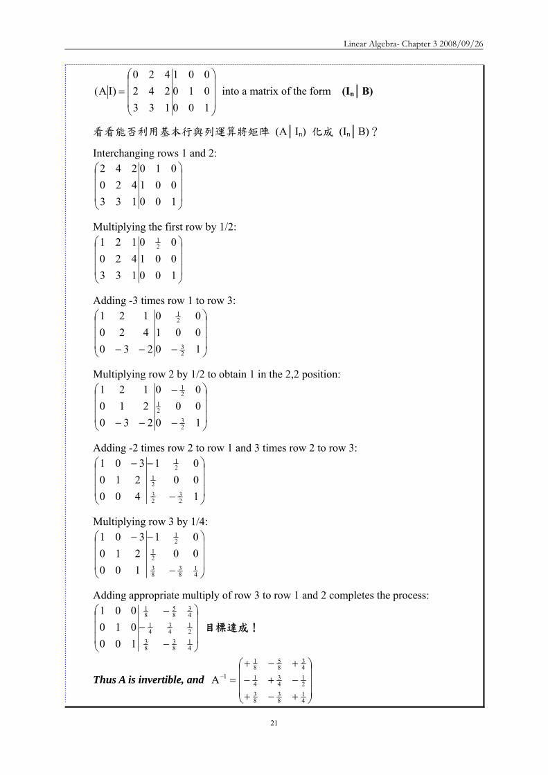
Linear Algebra- Chapter 3 20080926
21
⎟⎟⎟
⎠
⎞
⎜⎜⎜
⎝
⎛=
100010001
133242420
)IA( into a matrix of the form (InB)
看看能否利用基本行與列運算將矩陣 (AIn) 化成 (InB)
Interchanging rows 1 and 2
⎟⎟⎟
⎠
⎞
⎜⎜⎜
⎝
⎛
100001010
133420242
Multiplying the first row by 12
⎟⎟⎟
⎠
⎞
⎜⎜⎜
⎝
⎛
10000100
133420121 2
1
Adding -3 times row 1 to row 3
⎟⎟⎟
⎠
⎞
⎜⎜⎜
⎝
⎛
minusminusminus 1000100
230420121
23
21
Multiplying row 2 by 12 to obtain 1 in the 22 position
⎟⎟⎟
⎠
⎞
⎜⎜⎜
⎝
⎛
minus
minus
minusminus 100000
230210121
23
21
21
Adding -2 times row 2 to row 1 and 3 times row 2 to row 3
⎟⎟⎟
⎠
⎞
⎜⎜⎜
⎝
⎛
minus
minusminus
10001
400210301
23
2321
21
Multiplying row 3 by 14
⎟⎟⎟
⎠
⎞
⎜⎜⎜
⎝
⎛
minus
minusminus
41
83
8321
21
0001
100210301
Adding appropriate multiply of row 3 to row 1 and 2 completes the process
⎟⎟⎟
⎠
⎞
⎜⎜⎜
⎝
⎛
minusminus
minus
41
83
83
21
43
41
43
85
81
100010001
目標達成
Thus A is invertible and ⎟⎟⎟
⎠
⎞
⎜⎜⎜
⎝
⎛
+minus+minus+minus+minus+
=minus
41
83
83
21
43
41
43
85
81
1A
Linear Algebra- Chapter 3 20080926
22
EXAMPLE 6
We determine whether the matrix ⎟⎟⎟
⎠
⎞
⎜⎜⎜
⎝
⎛minus=451112
121A is invertible and if it is we
compute its inverse
A 是否為可逆矩陣
We attempt to use elementary row operations to transfer
⎟⎟⎟
⎠
⎞
⎜⎜⎜
⎝
⎛minus=
100010001
451112
121)IA( into a matrix of the form (InB)
看看能否利用基本行與列運算將矩陣 (AIn) 化成 (InB)
Adding -2 times row 1 to row 2 and -1 times row 1 to row 3 then addig row 2 to row
3
⎟⎟⎟
⎠
⎞
⎜⎜⎜
⎝
⎛minus
100010001
451112
121
⎟⎟⎟
⎠
⎞
⎜⎜⎜
⎝
⎛
minusminusminusminus
101012001
330330
121
⎟⎟⎟
⎠
⎞
⎜⎜⎜
⎝
⎛
minusminusminusminus
113012001
000330
121
is a matrix with row whose first 3 entries are zeros Therefore A is not invertible
最後一列前 3 個元素均為 0
EXAMPLE 7 Let T P2(R) P2(R) be defined by T(f(x)) = f(x)+frsquo(x)+frdquo(x) where frsquo(x) and frdquo(x)
denote the first and second derivatives of f(x) We use Corollary 1 to Theorem 218 to test
T for invertibility and compute the inverse if T is invertible Taking β=1 x x2 to be the
standard ordered basis of P2(R) we have
令 T P2(R) P2(R) 為線性轉換且定義為 T(f(x)) = f(x)+frsquo(x)+frdquo(x)利用
Corollary 1 to Theorem 218 來測試 T 是否可逆並計算其逆轉換取 β=1 x x2為
P2(R)的標準有序基底
T(1) = 1 = 1bull1+0bullx+0bullx2
T(x) = 1+x = 1bull1+1bullx+0bullx2
Linear Algebra- Chapter 3 20080926
23
T(x2) = 2+2x+x2 = 2bull1+2bullx+1bullx2
⎟⎟⎟
⎠
⎞
⎜⎜⎜
⎝
⎛=β
100210211
[T] 稱為 T 相對有序基底 β的座標向量
依據 Corollary 1 to Theorem 218 T 可逆『若且唯若』 β[T] 可逆且
1-1 )[T](][T minusββ =
Using the method of Examples 5 and 6 we can show that β[T] is invertible with
inverse
⎟⎟⎟
⎠
⎞
⎜⎜⎜
⎝
⎛minus
minus=minus
β
100210
011)([T] 1
Thus T is is invertible and βminusminus
β = ][T)([T] 11 Hence by Theorem 214 we have
⎟⎟⎟
⎠
⎞
⎜⎜⎜
⎝
⎛minusminus
=⎟⎟⎟
⎠
⎞
⎜⎜⎜
⎝
⎛
⎟⎟⎟
⎠
⎞
⎜⎜⎜
⎝
⎛minus
minus=++ β
minus
2
21
10
2
1
02
2101
aa2aaa
aaa
100210
011)]xaxa(a[T
Therefore T-1(a0+a1x+a2x2) = (a0-a1)+(a1-2a2)x+a2x2 Corollary 1 to Theorem 218 Let V be finite-dimensional vector space with an ordered basis β and let T V V be linear Then T is invertible if and only if β[T] is invertible
Furthermore 1-1 )[T](][T minusββ = V 為有限維度的向量空間β 是 V 的有序基底令 T
V V 為線性轉換 T 為可逆的『若且唯若』條件為 β[T] 可逆再者
1-1 )[T](][T minusββ =
Theorem 214 Let V and W be finite-dimensional vector spaces having ordered bases β and γ respectively and let T V W be linear Then for each uisinV we have β
γβγ = [u][T][T(u)]
V 與 W 為有限維度的向量空間β 與 γ分別 V 與 W 的有序基底令 T V W 為線
性轉換則 V 中的 u 映至 W 的結果 T(u) 相對於有序基底 γ 的座標向量為
βγβγ = [u][T][T(u)]
Invertible and Inverse of MATRIX Let A be an n times n matrix If a matrix B can be found such that AB = BA = In then A is
Linear Algebra- Chapter 3 20080926
24
said to be invertible and B is called the inverse of A (denote B = A-1 and A-k=(A-1)k )
If such a matrix B does not exist then A has no inverse
EXAMPLE
⎥⎦
⎤⎢⎣
⎡=
4321
A and ⎥⎦
⎤⎢⎣
⎡minus
minus=
21
23
12B
221
23
221
23
I1001
432112
BA
I100112
4321
AB
=⎥⎦
⎤⎢⎣
⎡=⎥
⎦
⎤⎢⎣
⎡⎥⎦
⎤⎢⎣
⎡minus
minus=
=⎥⎦
⎤⎢⎣
⎡=⎥
⎦
⎤⎢⎣
⎡minus
minus⎥⎦
⎤⎢⎣
⎡=
Thus AB = BA = I2 proving that the matrix A has inverse B
Theorem The inverse of an invertible matrix is unique
Let B and C be inverse of A
Thus AB = BA = In and AC = CA = In
Multiply both sides of the equation AB = In by C
C(AB) = CIn (CA)B = C
InB = C B = C
Thus an invertible matrix has only one inverse
How to find AHow to find A--11
Based on the GaussBased on the Gauss--Jordan algorithmJordan algorithmLet A be an invertible matrix Then AALet A be an invertible matrix Then AA--11=I=Inn
Let the columns of Let the columns of AA--11 be be XX11 XX22 helliphellip XXnn and the columns of I and the columns of Inn be be CC11CC22helliphellipCCnn
Find AFind A--11 by finding by finding XX11 XX22 helliphellip XXnn Write the equation AAWrite the equation AA--11=I=Inn in the formin the form
[ ] [ ]n21nn211 CCCI XXXALet LL ==minus
[ ] [ ][ ] [ ]n21n21
n21n21
CCCAXAXXACCCXXXALL
LL
=rArr=
nn2211 CAXCAX CAX === LThus
How to find AHow to find A--11
Solving these systems by using Gauss-Jordan elimination on the large augmented matrix [AC1 C2hellipCn]
Thus when A-1 exits
[ ] [ ] [ ] 1n
1nn ABwhereBIAIIA minusminus ==asympasympL
If the reduced echelon form of [If the reduced echelon form of [AIAInn] is computed and ] is computed and the first part is not of the form Ithe first part is not of the form Inn then A has no inversethen A has no inverse
[ ][ ]n21n
n21
XXXI CCCAmatrix augmented
LL
L
asympasymp
Linear Algebra- Chapter 3 20080926
25
Example Example 1212
⎥⎥⎥
⎦
⎤
⎢⎢⎢
⎣
⎡
minusminusminusminusminus
=100531010532001211
]IA[ 3
⎥⎥⎦
⎤
⎢⎢⎣
⎡minusminusminus
minusminus
+minus+
asymp
101320012110001211
1RR1R3
2)(R2
⎥⎥⎦
⎤
⎢⎢⎣
⎡minus
minusminusminusasymp
101320012110001211
R2)1(
⎥⎥⎥
⎦
⎤
⎢⎢⎢
⎣
⎡
minusminusminusminusminus
=531532211
ADetermine the inverse of
Example Example 2222
⎥⎥⎦
⎤
⎢⎢⎣
⎡
minusminusminusminus
minus++asymp
123100012110013101
R2)2(R3R2R1
⎥⎥⎦
⎤
⎢⎢⎣
⎡
minusminusminus
minus++asymp
123100135010010001
R3)1(R2R3R1
123135110
A 1
⎥⎥⎥
⎦
⎤
⎢⎢⎢
⎣
⎡
minusminusminus=minus
⎥⎥⎦
⎤
⎢⎢⎣
⎡
minusminus
minus
+minus+asymp
135000011210012301
3R2R3R2)1(R1
ExampleExampleDetermine the inverse of
⎥⎥⎦
⎤
⎢⎢⎣
⎡
minus=
412721511
A
⎥⎥⎦
⎤
⎢⎢⎣
⎡
minus=
100412010721001511
][ 3IA
⎥⎥⎦
⎤
⎢⎢⎣
⎡
minusminusminusminus
minus+minus+asymp
102630011210001511
R1)2(R31)R1(R2
There is no need to proceed further There is no need to proceed further The reduced echelon form cannot have a one in the (3 3) locatioThe reduced echelon form cannot have a one in the (3 3) location n
The reduced echelon form cannot be of the form [IThe reduced echelon form cannot be of the form [Inn B] B] Thus Thus AAndashndash11 does not existdoes not exist
Properties of Matrix InverseProperties of Matrix Inverse
Let Let AA and and BB be invertible matrices andbe invertible matrices and cc a nonzero scalar a nonzero scalar ThenThen
AA =minusminus 11)( 111 1)( 2 minusminus = A
ccA
111)( 3 minusminusminus = ABAB
nn AA )()( 4 11 minusminus =tt AA )()( 5 11 minusminus =
Color Models Color Models 1212
A color model in the context of graphics is a method of A color model in the context of graphics is a method of implementing colorsimplementing colorsThe common used models include RGB model and YIQ modelThe common used models include RGB model and YIQ modelThe RGB model is used in computer monitors and the YIQ model The RGB model is used in computer monitors and the YIQ model is used in television screensis used in television screensAn RGB computer signal can be converted to a YIQ television An RGB computer signal can be converted to a YIQ television signal using the matrix transformationsignal using the matrix transformation
⎥⎥⎥
⎦
⎤
⎢⎢⎢
⎣
⎡
⎥⎥⎥
⎦
⎤
⎢⎢⎢
⎣
⎡
minusminusminus=
⎥⎥⎥
⎦
⎤
⎢⎢⎢
⎣
⎡
BGR
311523212321275596
114587299
QIY
YIQgtRGBYIQgtRGB
Color Models Color Models 2222
A signal is converted from a television screen to a computer monA signal is converted from a television screen to a computer monitor itor using inverse of the above matrixusing inverse of the above matrix
⎥⎥⎥
⎦
⎤
⎢⎢⎢
⎣
⎡
⎥⎥⎥
⎦
⎤
⎢⎢⎢
⎣
⎡
minusminusminus=
⎥⎥⎥
⎦
⎤
⎢⎢⎢
⎣
⎡rArr
⎥⎥⎥
⎦
⎤
⎢⎢⎢
⎣
⎡
⎥⎥⎥
⎦
⎤
⎢⎢⎢
⎣
⎡
minusminusminus=
⎥⎥⎥
⎦
⎤
⎢⎢⎢
⎣
⎡minus
QIY
0751108116472721
6209561
BGR
QIY
311523212321275596
114587299
BGR 1
CryptographyCryptography 密碼學密碼學 1212
Cryptography is the process of coding and decoding messagesCryptography is the process of coding and decoding messagesThe technique can be traced back to the ancient Greeks Today The technique can be traced back to the ancient Greeks Today governments use sophisticated methods of coding and decoding governments use sophisticated methods of coding and decoding messagesmessagesOne type of code that is extremely difficult to break makes use One type of code that is extremely difficult to break makes use of a of a large matrix to encode a message large matrix to encode a message The receiver of the message decodes it using the inverse of the The receiver of the message decodes it using the inverse of the matrixmatrixThe first matrix is called the encoding matrix and its inverse The first matrix is called the encoding matrix and its inverse is is called the decoding matrixcalled the decoding matrix
Cryptography Cryptography 密碼學密碼學 2222
A A-1Message
Encoding MatrixEncoding Matrix
Decoded MessageTransmission
Decoding MatrixDecoding Matrix
Linear Algebra- Chapter 3 20080926
26
Example Example 1212
Let the message be Let the message be BUY IBM STOCKBUY IBM STOCKAnd the encoding matrix beAnd the encoding matrix be
⎥⎥⎥
⎦
⎤
⎢⎢⎢
⎣
⎡ minusminusminus
434110433
B U Y B U Y -- I B M I B M -- S T O C KS T O C K2 21 25 27 9 2 13 27 19 20 15 3 112 21 25 27 9 2 13 27 19 20 15 3 11
⎥⎥⎥
⎦
⎤
⎢⎢⎢
⎣
⎡ minusminusminusminusminus=
⎥⎥⎥
⎦
⎤
⎢⎢⎢
⎣
⎡
⎥⎥⎥
⎦
⎤
⎢⎢⎢
⎣
⎡ minusminusminus
2331372091431715418461146
222117196116169
27319225271527921112013272
434110433
EncodingEncoding
Example Example 2222
Let the message be Let the message be BUY IBM STOCKBUY IBM STOCKAnd the decoding matrix beAnd the decoding matrix be
⎥⎥⎥
⎦
⎤
⎢⎢⎢
⎣
⎡
minusminus 334344101
B U Y B U Y -- I B M I B M -- S T O C KS T O C K2 21 25 27 9 2 13 27 19 20 15 3 112 21 25 27 9 2 13 27 19 20 15 3 11
⎥⎥⎥
⎦
⎤
⎢⎢⎢
⎣
⎡=
⎥⎥⎥
⎦
⎤
⎢⎢⎢
⎣
⎡ minusminusminusminusminus
⎥⎥⎥
⎦
⎤
⎢⎢⎢
⎣
⎡
minusminus 27319225271527921112013272
2331372091431715418461146
222117196116169
334344101
DecodingDecoding
3-3 Systems of Linear Equations ndash Theoretical Aspects
The system of equations
mnmn22m11m
2nn2222121
1nn1212111
bxaxaxa
bxaxaxabxaxaxa
=+++
=+++=+++
(S)
were aij and bi (1≦i≦m and 1≦j≦n) are scalars in a field F and x1 x2hellipxn are n
variables taking values in F is called a system of m linear equations in n unknows over the
field F
上式稱為佈於 Field F 含有 n 個未知數m 個線性方程式的系統或方程組(system
of m linear equations in n unknows)
The mtimesn matrix
⎟⎟⎟⎟⎟
⎠
⎞
⎜⎜⎜⎜⎜
⎝
⎛
=
mn2m1m
n22221
n11211
aaa
aaaaaa
A is called the coefficient matrix of the
system (S)(係數矩陣) If we let
⎟⎟⎟⎟⎟
⎠
⎞
⎜⎜⎜⎜⎜
⎝
⎛
=
n
2
1
x
xx
x and
⎟⎟⎟⎟⎟
⎠
⎞
⎜⎜⎜⎜⎜
⎝
⎛
=
m
2
1
b
bb
b Then the system (S) may
be rewritten as a single matrix equation Ax = b(單一矩陣方程式)
To exploit the results that we have developed we often consider a system of linear
equations as a single matrix equation
Linear Algebra- Chapter 3 20080926
27
A solution to the system (S) is an n-tuple n
n
2
1
F
s
ss
s isin
⎟⎟⎟⎟⎟
⎠
⎞
⎜⎜⎜⎜⎜
⎝
⎛
= such that As = b The set of
all solutions to the system (S) is called the solution set of the system(解集合) System (S)
is called consistent(相容) if its solution set is nonempty otherwise it is called
inconsistent(不相容)
方程組(S)的解為一 n 序組該序組可以使 As = b方程組的所有解所成的集合
稱為該方程組的解集合(Solution set)方程組的解集合非空集合者稱為「相容」解
集合空集合者稱為「不相容」
EXAMPLE 1
Consider 6x2xx1xx3x2
321
321
=+minus=++
that is ⎟⎟⎠
⎞⎜⎜⎝
⎛=
⎟⎟⎟
⎠
⎞
⎜⎜⎜
⎝
⎛
⎟⎟⎠
⎞⎜⎜⎝
⎛minus 6
1
xxx
211132
3
2
1
(以矩陣表示)
This system has many solutions such as ⎟⎟⎟
⎠
⎞
⎜⎜⎜
⎝
⎛minus=
726
s and ⎟⎟⎟
⎠
⎞
⎜⎜⎜
⎝
⎛
minusminus=
34
8s
Consider 1xx0xx
21
21
=+=+
that is ⎟⎟⎠
⎞⎜⎜⎝
⎛=⎟⎟
⎠
⎞⎜⎜⎝
⎛⎥⎦
⎤⎢⎣
⎡10
xx
1111
2
1
顯然地方程組無解
We begin our study of system of linear equations by examining the class of
homogeneous system of linear equations 先討論齊次方程組
DEFINITION 35 Homogeneous amp Nonhomogeneous
A system Ax=b of m linear equations in n unknowns is said to be homogeneous if b=0
Otherwise the system is said to be nonhomogeneous
方程組 Ax = bb = 0 稱為齊次方程組否則稱為非齊次方程組
Any homogeneous system has at least one solution namely the zero vector The next
result gives further information about the set of solutions to a homogeneous system
Linear Algebra- Chapter 3 20080926
28
齊次方程組至少有一個解那就是『零向量』
Theorem 38 Let Ax = 0 be a homogeneous system of m linear equations in n unknowns over a field
F Let K denote the set of all solutions to Ax = 0 Then K = N(LA) hence K is a subspace
of Fn of dimension n - rank(LA) = n- rank(A)
令 Ax = 0 代表一佈於 Field 含有 n 個未知數m 個線性方程式的方程組若令
K 代表該方程組的解集合(Solution set)則 K = N(LA)K 為 Fn 內的子空間且其維
度為 n ndash rank (LA) = n - rank(A)
【Proof】
Clearly K = sisinFn As = 0 = N(LA) The second part now follows from the
dimension theorem
Nullity(T)+rank(T) = dim(V)
Nullity (LA) = dim (Fn) ndashrank (LA ) = n ndash rank (A)
DEFINTION 27 Let V and W be vector space and let T V W be linear We define
the null space (or kernel) N(T) of T to be the set of all vectors x in V such that T(x) = 0
that is N(T) = xisinV T(x) = 0 V 與 W 為向量空間且 T V W 為線性轉換定義
線性轉換 T 的 Null space 為 V 內所有滿足 T(x) = 0 的向量 x 所形成的集合註記為
N(T)Null space 的元素 x 經線性轉換 T 轉換後所對應的「像」為 0意即 T(x) = 0
Null space 內的元素的「像」皆為 0
DEFINITION 217 Let A be an mtimesn matrix with entries from a field F We denote by LA
the mapping LA Fn Fm defined by LA(x) = Ax (the matrix product A and x) for each
column vector xisinFn We call LA a left-multiplication transformation 令 A 是 mtimesn
的矩陣所有元素均來自 FLA 為 Fn 映至 Fm的線性轉換並定義為 LA(x) = Ax其中
x 為行向量(Column vector)且 xisinFnLA被稱為左乘法轉換
Theorem 23 (Dimension Theorem) Let V and W be vector spaces and let T V W be
linear If V is finite-dimensional then Nullity(T) + rank(T) = dim(V) T 的核次數
(Nullity)與秩(Rank)的和等於定義域的維度 dim(V)
Corollary Let Ax = 0 be a homogeneous system of m linear equations in n unknowns over a field
Linear Algebra- Chapter 3 20080926
29
F If m lt n the system Ax = 0 has a nonzero solution
令 Ax = 0 代表一佈於 Field 含有 n 個未知數m 個線性方程式的方程組若 m
lt n則該方程組具有一非零解
【Proof】
Suppose that m lt n Then rank(A) = rank (LA)≦m Hence dim(K) = n - rank(LA) ≧
n ndash m gt 0 where K = N(LA) Since dim(K) gt 0 Kne 0 Thus there exists a nonzero
vector sisinK so s is a nonzero solution to Ax = 0
設 m lt n則 rank(A) = rank (LA) ≦ m依據 Theorem 38K = sisinFn As = 0
= N(LA) = dim(K) = n - rank(LA) ≧ n ndash m gt 0表示 dim(K) gt 0Kne 0故存在非
零向量 s使得 Ax = 0
EXAMPLE 2
Consider 0xxx
0xx2x
321
321
=minusminus=++
Let ⎟⎟⎠
⎞⎜⎜⎝
⎛minusminus
=111
121A be the coefficient matrix of this system It is clear that rank(A)
= 2 If K is the solution set of this system then dim(K) = 3-2 = 1 Thus any nonzero
solution constitutes a basis for K
若 K 是方程組的解所組成的集合(簡稱為解集合)依 Theorem 38 得知 dim(K)
= 3 - 2 = 1因此任一非零解將形成 K 的基底
For example since ⎟⎟⎟
⎠
⎞
⎜⎜⎜
⎝
⎛minus32
1 is a solution to the given system
⎪⎭
⎪⎬
⎫
⎪⎩
⎪⎨
⎧
⎟⎟⎟
⎠
⎞
⎜⎜⎜
⎝
⎛minus32
1 is a basis for
K Thus any vector in K is of the form ⎟⎟⎟
⎠
⎞
⎜⎜⎜
⎝
⎛minus=
⎟⎟⎟
⎠
⎞
⎜⎜⎜
⎝
⎛minus
t3t2
t
32
1t where tisinR
例如因⎟⎟⎟
⎠
⎞
⎜⎜⎜
⎝
⎛minus32
1是方程組的一個解故
⎪⎭
⎪⎬
⎫
⎪⎩
⎪⎨
⎧
⎟⎟⎟
⎠
⎞
⎜⎜⎜
⎝
⎛minus32
1 為 K 的基底K 內的任一向量均
具有如下形式
⎟⎟⎟
⎠
⎞
⎜⎜⎜
⎝
⎛minus=
⎟⎟⎟
⎠
⎞
⎜⎜⎜
⎝
⎛minus
t3t2
t
32
1t
Linear Algebra- Chapter 3 20080926
30
We now turn to the study of nonhomogeneous systems Our next result shows that the
solution set of a nonhomogeneous system Ax = b can be described in terms of the solution of
the homogeneous system Ax = 0 We refer to the equation Ax = 0 as the homogeneous system
corresponding to Ax = b
以下將進一步探討「非齊次方程組」非齊次方程組 Ax = b 的解集合可利用齊次方
程組 Ax = 0 的解來加以說明因此我們可將 Ax = 0 視為 Ax = b 的齊次方程組
Theorem 39 Let K be the solution set of a system of linear equations Ax = b and let KH be the
solution set of the corresponding homogeneous system Ax = 0 Then for any solution s to
Ax = b K =s + KH = s+k kisinKH
設 K 為線性方程組 Ax = b 的解集合且 KH為對應的齊次方程組的解集合則
對 Ax = b 的任一個解 s 而言K =s + KH = s+k kisinKH
【Proof】
Let s be any solution to Ax = b
We must show that K =s + KH
If wisinK then Aw = b Hence
A(w - s) = Aw ndash As = b ndash b = 0
So w - sisinKH
Thus there exists kisinKH such that w - s = k
It follows that w = s + k isin s +KH and therefore Ksube s +KH
Conversely suppose that wisins +KH then w = s + k for some kisinKH
But then Aw = A(s + k) = As + Ak = b + 0 = b so wisinK
Therefore s +KHsubeK and thus K=s +KH
令 s 為 Ax = b 的任一個解我們必須證明「K =s + KH」
若 wisinK則 Aw = b(即 w 為 Ax = b 的解)
於是 A(w - s) = Aw ndash As = b ndash b = 0
所以 w - sisinKH(即 w-s 為 Ax = 0 的解)
w - s 既然是 KH的元素表示有一元素 kisinKH使得 w - s = kw = s + k
w = s + kisins +KH
Linear Algebra- Chapter 3 20080926
31
因此 Ksube s +KH
反之假設 wisins +KH則 KH中存在一元素 k(kisinKH)使得 w = s + k
因 Aw = A(s + k) = As + Ak = b + 0 = b
故 wisinK 是 Ax = b 的解
因此s +KHsubeK
總結K=s +KH
EXAMPLE 3
Consider 4xxx7xx2x
321
321
minus=minusminus=++
The corresponding homogeneous system is the system in Example 2 It is easily
verified that ⎟⎟⎟
⎠
⎞
⎜⎜⎜
⎝
⎛=
411
s is a solution to the preceeding nonhomogeneous system So the
solution set of the system is ⎪⎭
⎪⎬
⎫
⎪⎩
⎪⎨
⎧isin
⎟⎟⎟
⎠
⎞
⎜⎜⎜
⎝
⎛minus+
⎟⎟⎟
⎠
⎞
⎜⎜⎜
⎝
⎛= Rt
32
1t
411
K by Theorem 39
⎟⎟⎟
⎠
⎞
⎜⎜⎜
⎝
⎛=
411
s 是非齊次方程組 Ax = b 的解
⎟⎟⎟
⎠
⎞
⎜⎜⎜
⎝
⎛minus32
1是齊次方程組的解
依據 Theorem 39 得知線性方程組 Ax = b 的解集合⎪⎭
⎪⎬
⎫
⎪⎩
⎪⎨
⎧isin
⎟⎟⎟
⎠
⎞
⎜⎜⎜
⎝
⎛minus+
⎟⎟⎟
⎠
⎞
⎜⎜⎜
⎝
⎛= Rt
32
1t
411
K
The following theorem will provide us with a means of computing solutions to certain
system of linear equations
Theorem 310~311 提供計算線性方程組的解的方法
Theorem 310 Let Ax = b be a system of n linear equations in n unknowns If A is invertible then the
Linear Algebra- Chapter 3 20080926
32
system has exactly one solution namely A-1b Conversely if the system has exactly one
solution then A is invertible
令 Ax = b 為含 n 個未知數n 個線性方程式的方程組若 A 為可逆則方程組
恰有一個解解為 A-1b反之若該方程組恰有一個解則 A 為可逆
【Proof】
Suppose that A is invertible
Substituting A-1b into system we have A(A-1b)=( AA-1)b = b
Thus A-1b is a solution
If s is an arbitrary solution then As = b
Multiplying both sides by A-1 gives s= A-1b
Thus the system has one and only one solution namely A-1b
假設 A 為可逆將 A-1b 代入方程組可得 A(A-1b)=( AA-1)b = b
故 A-1b 確為方程組的解
若 s 為方程組的任意解則 As = b
兩邊乘上 A-1可得 s= A-1b
因此方程組僅有唯一的解 A-1b
Conversely suppose that the system has exactly one solution s
Let KH denot the solution set for the corresponding homogeneous system Ax = 0
By Theorem 39 s = s + KH But it is so only if KH = 0 Thus N(LA) = 0 and
hence A is invertible
反之假設方程組恰有一個解 s
令 KH為相對應齊次方程組 Ax = 0 的解集合
依據 Theorem 39要能s = s + KH唯有 KH = 0
KH = 0即表示 N(LA) = 0故 A 為可逆
EXAMPLE 4 Consider the following system of three linear equations in three unknowns
1xx3x33x2x4x2
2x4x2
321
321
32
=++=++
=+
In Example 5 of Section 32 we compute the inverse of the coefficient matrix A of
this system Thus the system has exactly one solution namely
Linear Algebra- Chapter 3 20080926
33
⎟⎟⎟
⎠
⎞
⎜⎜⎜
⎝
⎛=
133242420
A⎟⎟⎟
⎠
⎞
⎜⎜⎜
⎝
⎛
+minus+minus+minus+minus+
=minus
41
83
83
21
43
41
43
85
81
1A
⎟⎟⎟
⎠
⎞
⎜⎜⎜
⎝
⎛
minus+minus
=⎟⎟⎟
⎠
⎞
⎜⎜⎜
⎝
⎛
⎟⎟⎟
⎠
⎞
⎜⎜⎜
⎝
⎛
+minus+minus+minus+minus+
==⎟⎟⎟
⎠
⎞
⎜⎜⎜
⎝
⎛minus
814587
41
83
83
21
43
41
43
85
81
1
3
2
1
132
bAxxx
Theorem 311 Let Ax = b be a system of linear equations Then the system is consistent (相容)if
and only if rank(A) = rank (A∣b) Matrix (A b) is called the augmented matrix o∣ f the
system Ax = b
令 Ax = b 為線性方程式方程組則此方程組至少有一個解的『若且唯若』條件
為 rank(A) = rank (A∣b) 矩陣(A∣b)稱為方程組 Ax = b 的增廣矩陣
【Proof】
To say that Ax = b has a solution is equivalent to saying that bisinR(LA)
In the proof of Theorem 35 we saw that R(LA ) = span(a1 a2 an) the span of the
column of A
Thus Ax = b has a solution if and only if bisinspan(a1 a2 an)
But bisinspan(a1 a2 an) if and only if span(a1 a2 an) = span(a1 a2 an b)
This last statement is equivalent to
dim (span(a1a2an)) = dim (span(a1a2an b))
So by Theorem 35 the preceeding equation reduces to rank(A) = rank (A∣b)
Ax = b 有一解相當於 bisinR(LA)即 b 屬於線性轉換 LA的 Range
在 Theorem 35 的證明中提到 R(LA ) = span(a1a2an)aj 為 A 的第 j 個行
(Column)即線性轉換 LA 的 Range 係由矩陣 A 的行(Column)所生成
因此 Ax = b 要有一個解的『若且唯若』條件為 bisinspan(a1 a2 an)
至於 bisinspan(a1 a2 an)之條件
bisinspan(a1a2an) 的『若且唯若』條件為 span(a1a2an) = span(a1a2an
b)
其條件相當於
Linear Algebra- Chapter 3 20080926
34
dim (span(a1a2an)) = dim (span(a1a2an b))
依據 Theorem 35該條件可簡化為 rank(A) = rank (A∣b)
Theorem 35 The rank of any matrix equals the maximum number of its linearly
independent columns that is the rank of a matrix is the dimension of the subspace
generated by its column任一矩陣的 Rank 等於其最大線性獨立行向量數目即矩陣的
Rank 是由矩陣的行向量生成的子空間的維度【LA Fn Fm】
EXAMPLE 5 Recall the system of equations
1xx0xx
21
21
=+=+
Since ⎟⎟⎠
⎞⎜⎜⎝
⎛=
1111
A and ⎟⎟⎠
⎞⎜⎜⎝
⎛=
111011
)bA(
rank(A) = 1 and rank (A b) = 2∣
Because the two ranks are unequal the system has no solutions
矩陣 A 與增廣矩陣(A∣b) 的 Rank 不同故方程組沒有解
EXAMPLE 6 We can use Theorem 311 to determine whether (3 3 2) is in the range of the linear
transformation T R3 R3 defined by T(a1 a2 a3) = (a1+a2+a3 a1-a2+a3 a1+a3)
利用 Theorem 311 來判斷 (3 3 2)是否在線性轉換 T 的 Range 中其中T R3
R3 定義為 T(a1 a2 a3) = (a1+a2+a3 a1-a2+a3 a1+a3)
Now (3 3 2)isinR(T) if and only if there exists a vector s = x1 x2 x3 in R3 such that
T(s)=(3 3 2) Such a vector s must be a solution to the system
2xx3xxx3xxx
31
321
321
=+=+minus=++
Since the ranks of the coefficient matrix and the augmented matrix of this system
are 2 and 3 respectively it follows that this system has no solutions Hence (3 3 2) notin
R(T)
(3 3 2)isinR(T) 的『若且唯若』的條件為存在一向量 s = x1 x2 x3isinR3 使得
T(s)=(3 3 2)
Linear Algebra- Chapter 3 20080926
35
向量 s 必須是 2xx3xxx3xxx
31
321
321
=+=+minus=++
的解
因係數矩陣⎟⎟⎟
⎠
⎞
⎜⎜⎜
⎝
⎛minus
101111111
的 Rank 為 2增廣矩陣⎟⎟⎟
⎠
⎞
⎜⎜⎜
⎝
⎛minus
233
101111111
的 Rank 為 3兩
者不相等故方程組無解(3 3 2) notin R(T)
Theorem 311 Let Ax = b be a system of linear equations Then the system is consistent
(相容)if and only if rank(A) = rank (A∣b) Matrix (A b) is called the ∣ augmented
matrix of the system Ax = b 令 Ax = b 為線性方程式方程組則此方程組至少有一個
解的『若且唯若』條件為 rank(A) = rank (A∣b) 矩陣(A∣b)稱為方程組 Ax = b 的
增廣矩陣
Application
In 1973 Wassily Leontief won the Nobel prize in economics for his work in developing
a mathematical model that can be used to describe various economic phenomena
1973 年Wassily Leontief 因研究一數學模式來描述各種經濟現象而獲頒諾貝爾經
濟獎
CLOSED MODEL
We begin by considering a simple society composed of three peoples (industries) ndash a
farmer who gows all the food a tailor who makes all the clothing and a carpenter who builds
all the housing We assume that each person sells to and buy from a central pool and that
everything produced is consumed Since no commodities either enter or leave the system this
case is referred to as the CLOSE MODEL
考慮一個單純社會的三種人生產食物的農夫製衣的裁縫師與蓋住屋的木匠
並假設採取集中聯營買賣且每一件產品皆付諸消費由於過程中沒有任何成品進入
或脫離這個系統所以稱為「封閉模式」
Each of these three individual consumes all three of the commodities produced in the
Linear Algebra- Chapter 3 20080926
36
society Suppose that the proportion of each of the commodities consumed by each person is
given in the following table
社會中每一位皆消費所生產的三種成品且每一種產品也都被三位所消費其消
費比例如下
食物 Food 衣物 Clothing 住屋 Housing
農夫 Farmer 040 020 020
裁縫師 Tailor 010 070 020
木匠 Carpenter 050 010 060
Let p1 p2 and p3 denote the incomes of the farmer tailor and carpenter respectively To
ensure that this society survives we require that the consumption of each individual equals
his or her income
令 p1p2 與 p3 分別表示農夫裁縫師與木匠的收入並為確保這個封閉社會可以
存活假設每一位的收入等於消費
Note that the farmer consumes 20 of the clothing Because the total cost of all clothing
is p2 the tailorrsquos income the amount spent by the farmer on clothing is 020 p2 Moreover the
amount spent by the farmer on food clothing and housing must equal the farmerrsquos income
and so we obtain the equation 040 p1 + 020 p2 + 030 p3 = p1
對農夫而言農夫的衣物消費佔 20然因所有衣物的消費總額 p2 等於裁縫師的
收入所以農夫在衣物上的消費為 020 p2且農夫在食物衣物與住屋的總消費要等
於農夫的收入 p1所以農夫的收入與消費關係式
040 p1 + 020 p2 + 020 p3 = p1
Similary equations describing the expenditures of the tailor and carpenter produce the
following system of linear equations
同理分別對裁縫師與木匠進行討論可獲得下列方程組
Linear Algebra- Chapter 3 20080926
37
040 p1 + 020 p2 + 020 p3 = p1
010 p1 + 070 p2 + 020 p3 = p2
050 p1 + 010 p2 + 060 p3 = p3
This system can be written as Ap = p
其中⎟⎟⎟
⎠
⎞
⎜⎜⎜
⎝
⎛=
3
2
1
ppp
p 且⎟⎟⎟
⎠
⎞
⎜⎜⎜
⎝
⎛=
600100500200700100200200400
A 稱為輸入-輸出(或消費)矩陣
(Input-output (or consumption) matrix)
Ap = p 稱為均衡條件(Equilibrium condition)
能否利用不等式 p ≦ p 來替代等式
At first it may seem reasonable to replace the equilibrium condition by the inequality
Ap ≦ p that is the requirement that consumption not exceed production But in fact Ap ≦ p implies that Ap = p in the closed model
For otherwise there exists a k for which
sumgt
jjkjk pAp
Hence since the columns of A sum to 1
sumsumsumsum ==gt
jj
i jjij
ii ppAp which is a contradiction (出現矛盾)
答案是在封閉系統中Ap ≦ p Ap = p
One solution to the homogeneous system (I ndash A) x = 0 which is equivalent to the
equilibrium condition is ⎟⎟⎟
⎠
⎞
⎜⎜⎜
⎝
⎛=
400350250
p
Linear Algebra- Chapter 3 20080926
38
齊次方程組(I ndash A) x = 0 或均衡條件的一個解為 ⎟⎟⎟
⎠
⎞
⎜⎜⎜
⎝
⎛=
400350250
p
We may interpret this to mean that the society survives if the farmer taior and carpenter
have incomes in the proportions 253540
⎟⎟⎟
⎠
⎞
⎜⎜⎜
⎝
⎛=
400350250
p 可以解釋為若農夫裁縫師與木匠收入比例為 253540則社會將
能生存下去
Theorem 312
Let A be an ntimesn input-output matrix having the form ⎟⎟⎠
⎞⎜⎜⎝
⎛=
EDCB
A where D is a 1times(n-
1) positive vector and C is an (n-1)times1 positive vector Then (I-A)x = 0 has a one-
dimensional solution set that is generated by a nonnegative vector
設 A 為 ntimesn 輸入-輸出矩陣 ⎟⎟⎠
⎞⎜⎜⎝
⎛=
EDCB
A 其中D 為 1times(n-1)正向量C 為
(n-1)times1 正向量則(I-A)x = 0 具有一維解集合且該解集合係由一非負向量所生成
Any input-output matrix with all positive entries satisfies the hypothesis of this theorem
任何輸入-輸出矩陣滿足 Theorem 312 的基本假設條件例如
⎟⎟⎟
⎠
⎞
⎜⎜⎜
⎝
⎛=
02502503502500650500750
A
OPEN MODEL
In the OPEN MODEL we assume that there is an outside demand for each of the
commodities produced Returning to our simple society let x1 x2 and x3 be the monetary
values of food clothing and housing produced with respective outside demands d1 d2 and d3
Let A be the 3times3 matrix such that Aij represents the amount of commodity i required to
Linear Algebra- Chapter 3 20080926
39
produce one monetary unit of commodity j Then the value of the surplus of food in the
society is x1 ndash (A11x1+A12x2+A13x3) that is the value of food produced minus the value of
food consumed while producing the three commodities The assumption that everything
produced is consumed gives us a similar equilibrium condition for the open model namely
that the surplus of each of the three commodities must equal the corresponding outside
demands Hence i
3
1jjiji dxAx =minussum
=
for j=1 2 3
在「開放模式」中我們假設每一產品皆有外來的需求在前述的單純社會裡
令 x1x2 與 x3 分別代表食物衣物與住屋的貨幣價值d1d2 與 d3 為食物衣物與住
屋的外來需求價值令 A 為 3times3 矩陣Aij 表示生產『一個貨幣單位』的產品 j 所需要
的產品 i 的價值於是此社會中食物的盈餘價值為 x1 ndash (A11x1+A12x2+A13x3)即食物的
價值減去生產食物衣物與住屋所需消耗的食物的價值意即生產出來的食物價值扣
掉用去生產食物衣物與住屋所消耗掉的價值)(A11A12A13 為生產一個貨幣單位
的食物 1衣物 2 與住屋 3 所需消耗的食物 1 數量A12x2 表示生產貨幣價值為 x2的衣物
所需要的食物價值)對每一種產品而言其盈餘價值等於外來的需求價值於是
i
3
1jjiji dxAx =minussum
=
for j=123
Suppose that 30 cents worth of food 10 cents worth of clothing and 30 cents worth of
housing are required for the production of $1 worth of food Similar suppose that 20 cents
worth of food 40 cents worth of clothing and 20 cents worth of housing are required for the
production of $1 worth of clothing Finally suppose that 30 cents worth of food 10 cents
worth of clothing and 30 cents worth of housing are required for the production of $1 worth
of housing Then the input-output matrix is
⎟⎟⎟
⎠
⎞
⎜⎜⎜
⎝
⎛=
300200300100400100300200300
A
假設生產價值 1 元的食物需要價值 30 分的食物(A11 = 03)價值 10 分的衣物
(A21 = 01)及價值 30 分的住屋(A31 = 03)生產價值 1 元的衣物需要價值 20 分的
食物(A12 = 02)價值 40 分的衣物(A22 = 04)及價值 20 分的住屋(A32 = 02)生
Linear Algebra- Chapter 3 20080926
40
產價值 1 元的住屋需要價值 30 分的食物(A13 = 03)價值 10 分的衣物(A23 = 01)
及價值 30 分的住屋(A33 = 03)於是輸入輸出矩陣 A 為
⎟⎟⎟
⎠
⎞
⎜⎜⎜
⎝
⎛=
300200300100400100300200300
A
若食物的外來需求值為 300 億元衣物為 200 億元住屋值為 1 百億元則
⎟⎟⎟
⎠
⎞
⎜⎜⎜
⎝
⎛=
⎟⎟⎟
⎠
⎞
⎜⎜⎜
⎝
⎛
⎟⎟⎟
⎠
⎞
⎜⎜⎜
⎝
⎛
minusminusminusminusminusminus
=minus=
minus
minus
700600900
100200300
700200300100600100300200300
d)AI(x
1
1
⎟⎟⎟
⎠
⎞
⎜⎜⎜
⎝
⎛=
700600900
x 表示要滿足外來需求必須生產的食物價值為 900 億元衣物價值為
600 億元住屋價值為 700 億元
Theorem
Let AX = Y be a system of n linear equations in n variables If Andash1 exists the
solution is unique and is given by X = Andash1Y
【Proof】
Substitute X = Andash1Y into the matrix equation
AX = A(Andash1Y) = (AAndash1)Y = InY = Y
The solution is unique
Let X1 be any solution thus AX1 = Y Multiplying both sides of this equation by Andash1
gives
Andash1AX1= Andash1Y InX1 = Andash1Y X1 = Andash1Y
Linear Algebra- Chapter 3 20080926
41
Example Example 1212
2x5x3x3x5x3x21x2x x
321
321
321
minus=++minus=minusminus=minusminus
⎥⎥⎥
⎦
⎤
⎢⎢⎢
⎣
⎡
minus=
⎥⎥⎥
⎦
⎤
⎢⎢⎢
⎣
⎡
⎥⎥⎥
⎦
⎤
⎢⎢⎢
⎣
⎡
minusminusminusminusminus
231
xxx
531532211
3
2
1
Solve the system of equations
This system can be written in the following matrix form
⎥⎥⎥
⎦
⎤
⎢⎢⎢
⎣
⎡
minus⎥⎥⎥
⎦
⎤
⎢⎢⎢
⎣
⎡
minusminusminusminusminus
=
⎥⎥⎥
⎦
⎤
⎢⎢⎢
⎣
⎡minus
231
531532211
xxx 1
3
2
1
If the matrix of coefficients is invertible the unique solutionIf the matrix of coefficients is invertible the unique solution isis
Example Example 2222
1 2 1 issolution unique The 321 =minus== xxx
⎥⎥⎥
⎦
⎤
⎢⎢⎢
⎣
⎡minus=
⎥⎥⎥
⎦
⎤
⎢⎢⎢
⎣
⎡
minus⎥⎥⎥
⎦
⎤
⎢⎢⎢
⎣
⎡
minusminusminus=
⎥⎥⎥
⎦
⎤
⎢⎢⎢
⎣
⎡
121
231
123135110
xxx
3
2
1
⎥⎥⎥
⎦
⎤
⎢⎢⎢
⎣
⎡
minusminusminus=
⎥⎥⎥
⎦
⎤
⎢⎢⎢
⎣
⎡
minusminusminusminusminus
=
minus
minus
123135110
531532211
A
1
1
The The LeontiefLeontief IO Model in IO Model in Economics Economics 1515
The Leontief input-output model is used to analyze the interdependence of economics Wassily Leontief received a Nobel Prize in 1973 for his work in thie fieldThe practical applications of this model have proliferated until it has now become a standard tool for investigating economic structures ranging from cities and corporation to states and countriesConsider an economics situation that involves ninterdependent industries The output of any one industry is needed as input by other industries and even possibly by the industry itself
The The LeontiefLeontief IO Model in IO Model in Economics Economics 2525
How a mathematical model involving a system of linear equations can be constructed to analyze such a situationAssume that each industry produces one commodity Let aij denote the amount of input of a certain commodity i to produce unit output of commodity j In our model let the amounts of input and output be measured in dollars Thus for example a34 = 045 means that 45 centsrsquo worth of commodity 3 is required to produce one dollarrsquos worth of commodity 4
The The LeontiefLeontief IO Model in IO Model in Economics Economics 3535
aij = amount of commodity i in one dollar of commodity jaij =生產一元價值的j產品需要耗用的i產品價值
The elements aij called input coefficients define a matrix A called the input-output matrix which describes the interdependence of the industriesExtending the model to include an open sector (all non-producing sectors) The product of industries may go not only into other producing industries but also into other non-producing sectors of the economy such as consumers and governments
The The LeontiefLeontief IO Model in IO Model in Economics Economics 4545
di = demand of the open sectors from industry ixi=total output of industry I necessary to meet demands of all n industries and the open sector
sectoropen of demand
nindustry of demand
2industry of demand
22
1industry of demand
11
industry ofoutput total
ininii
i
i dxaxaxax ++sdotsdotsdot++=
output ofportion sectoropen
output ofportion tryinterindusoutput total
DAXX +=Demand matrixDemand matrix
Output matrixOutput matrix
The The LeontiefLeontief IO Model in IO Model in Economics Economics 5555
Applying the model to the economy of a country X Applying the model to the economy of a country X represents the total output of each of the producing sectors represents the total output of each of the producing sectors of the economy and AX describes the contributions made of the economy and AX describes the contributions made by the various sectors to fulfilling the intersectional input by the various sectors to fulfilling the intersectional input requirements of the economyrequirements of the economyD is equal to (XD is equal to (X--AX) the difference between total output AX) the difference between total output X and industry transaction AXX and industry transaction AXD is thus the gross national product of the economyD is thus the gross national product of the economy
Example Example 1414
Consider an economy consisting of three industries having Consider an economy consisting of three industries having the following inputthe following input--output matrix output matrix AA Determine the output Determine the output levels required of the industries to meet the demands of levels required of the industries to meet the demands of the other industries and of the open sector in each casethe other industries and of the open sector in each case
in turn 321812
and 896
1612
9
5100
021
21
103
51
51
⎥⎥⎦
⎤
⎢⎢⎣
⎡
⎥⎥⎦
⎤
⎢⎢⎣
⎡
⎥⎥⎦
⎤
⎢⎢⎣
⎡=
⎥⎥⎥
⎦
⎤
⎢⎢⎢
⎣
⎡
= DA
The unit of The unit of DD are millions of dollarsare millions of dollars
Linear Algebra- Chapter 3 20080926
42
Example Example 2424
We wish to compute the output levels X that correspond to We wish to compute the output levels X that correspond to the various open sector demands D X is given by the the various open sector demands D X is given by the equation X = AX + D Rewritten as followsequation X = AX + D Rewritten as follows
X ndash AX = D rArr (I ndash A)X = D rArr X = (I ndash A) ndash1 D
⎥⎥⎥
⎦
⎤
⎢⎢⎢
⎣
⎡
=⎥⎥⎥
⎦
⎤
⎢⎢⎢
⎣
⎡
minus⎥⎥⎦
⎤
⎢⎢⎣
⎡=minus minus
minusminus
5400
021
21
103
51
54
5100
021
21
103
51
31
100010001
get We AI
⎥⎥⎥
⎦
⎤
⎢⎢⎢
⎣
⎡
=minus minus
4500
038
35
85
32
35
1)( AI
output ofingcorrespond valuesvarious
4500
038
35
85
32
35
)(
401020883957522133
32816189121269
)(
1
1
DAI
DAIX
minus
minus
minusuarruarruarruarruarruarruarr
⎥⎥⎦
⎤
⎢⎢⎣
⎡=
⎥⎥⎦
⎤
⎢⎢⎣
⎡
⎥⎥⎥
⎦
⎤
⎢⎢⎢
⎣
⎡
=minus=
Example Example 3434
By using Gauss-Jordan elimination
dollars of milliond are units The
40
15674
and 106629
209946
are 321812
and 896
1612
9
⎥⎥⎥
⎦
⎤
⎢⎢⎢
⎣
⎡
⎥⎥⎥
⎦
⎤
⎢⎢⎢
⎣
⎡
⎥⎥⎥
⎦
⎤
⎢⎢⎢
⎣
⎡
⎥⎥⎥
⎦
⎤
⎢⎢⎢
⎣
⎡
⎥⎥⎥
⎦
⎤
⎢⎢⎢
⎣
⎡
⎥⎥⎥
⎦
⎤
⎢⎢⎢
⎣
⎡
Example Example 4444
The output levels necessary to meet the demandsThe output levels necessary to meet the demands
IAAAIAI m =++++minus ))(( 2 L
mAAAIAI ++++=minus minus L21)(
Computing (IComputing (I--A) A) --11
1m
m2m2
m2
AI)AAAI(A)AAAI(I
)AAAI)(AI(
+minus=++++minus++++=
++++minusLL
L
NOTE 0A 1m rarr+
Population Movement Population Movement 1313
In 2000 58 million of people live in cities and 142 million of In 2000 58 million of people live in cities and 142 million of people people live in the surrounding suburbs Represent this information by tlive in the surrounding suburbs Represent this information by the he matrix matrix
The probability of a person staying in the city was 096 Thus tThe probability of a person staying in the city was 096 Thus the he probability of moving to the suburbs was 004 probability of moving to the suburbs was 004 The probability of a person moving to the city was 001 the The probability of a person moving to the city was 001 the probability of remaining in suburbia was 099probability of remaining in suburbia was 099
suburbcity
990040010960
suburbcity (to))from(
⎥⎦
⎤⎢⎣
⎡=P
⎥⎦
⎤⎢⎣
⎡=
14258
X0
City population in 2001 = people who remained from 2000 + peopleCity population in 2001 = people who remained from 2000 + peoplewho moved in from the suburbs = ( 096 who moved in from the suburbs = ( 096 timestimes 58 ) + (001 58 ) + (001 timestimes 142 ) = 142 ) = 571 million571 millionSuburban population in 2001 = people who moved in from the city Suburban population in 2001 = people who moved in from the city + people who stayed from 2000 = ( 004 + people who stayed from 2000 = ( 004 timestimes 58 ) + (099 58 ) + (099 timestimes 142 ) = 142 ) = 1429 million1429 millionCan arrive at these numbers using matrix multiplicationCan arrive at these numbers using matrix multiplication
⎥⎦
⎤⎢⎣
⎡=⎥
⎦
⎤⎢⎣
⎡⎥⎦
⎤⎢⎣
⎡==
9142157
14258
990040010960
PXX 01
Population Movement Population Movement 2323
Population Movement Population Movement 3333
Assume that the population flow represented by the matrix P is unchanged over the years The population distribution X2 after 2 years is given by X2 = P X1 = P2 X0 In general
Pn is called the n-step transition matrix The (ij)th element of Pngives the probability of going from state j to state i in n stepsFor example
in
ni XPX =+
suburbcity
960150040850
P
suburbcity (to))from(
4
⎥⎦
⎤⎢⎣
⎡=
The probability of living in the city in The probability of living in the city in 2000 and being in the suburbs 4 years 2000 and being in the suburbs 4 years later is 015later is 015
Markov ChainsMarkov Chains
The probabilities in the above model depend only on the The probabilities in the above model depend only on the current state of a person whether the person is living in the current state of a person whether the person is living in the city or in suburbiacity or in suburbiaThis type of model in which the probability of going from This type of model in which the probability of going from one state to another depends only on the current state one state to another depends only on the current state rather than on a more complete historical description is rather than on a more complete historical description is called a called a Markov chainMarkov chainMarkov chains are useful tools for scientists in many Markov chains are useful tools for scientists in many fields such as geneticsfields such as genetics
Linear Algebra- Chapter 3 20080926
43
GeneticsGenetics 1414
Genetics is the branch of biology that deals with Genetics is the branch of biology that deals with heredity heredity (遺傳)(遺傳) It is the study of units called It is the study of units called genes which determine the characteristics living genes which determine the characteristics living things inherit from their parents The inheritance things inherit from their parents The inheritance (遺傳)(遺傳)of such traitsof such traits(特徵)(特徵)as sex height eye as sex height eye color and hair color of human beings and such color and hair color of human beings and such traits as petaltraits as petal(花瓣)(花瓣) color and leaf shape of color and leaf shape of plants are governed by genesplants are governed by genesIn medicine agricultureIn medicine agriculturehelliphellip
GeneticsGenetics 2424
The traits of guinea pigsThe traits of guinea pigs(天竺鼠)(天竺鼠)are long hair and short hairare long hair and short hairThe length of hair is governed by a pair of gene which we denoteThe length of hair is governed by a pair of gene which we denote A A and aand aA guinea pig may have any one of the combination of AA A guinea pig may have any one of the combination of AA AaAa or or aaaa Each of these classes is called a genotypeEach of these classes is called a genotype(基因型)(基因型)The AA type guinea pig is indistinguishable in appearance from tThe AA type guinea pig is indistinguishable in appearance from the he AaAa type type ndashndash both have long hair both have long hair ndashndash whereas the whereas the aaaa type has short hairtype has short hairThe A gene is said to dominate the a geneThe A gene is said to dominate the a geneAn animal is called dominant An animal is called dominant (顯性)(顯性)if it has AA genes hybridif it has AA genes hybrid(混種)(混種) with with AaAa genes and recessive genes and recessive (隱性)(隱性)with with aaaa genesgenes
GeneticsGenetics 3434
When two guinea pigs are crossed the offspring inherits one genWhen two guinea pigs are crossed the offspring inherits one gene e from each parent in random mannerfrom each parent in random mannerGiven the genotype of the parents we can determine the Given the genotype of the parents we can determine the probabilities of the genotype of the offspringprobabilities of the genotype of the offspring
AA+AA AA+AA probabilities of AA probabilities of AA AaAa and and aaaa are 10and 0are 10and 0Aa+AAAa+AA probabilities of AA probabilities of AA AaAa and and aaaa are are frac12frac12 frac12frac12 and 0 and 0aa+AAaa+AA probabilities of AA probabilities of AA AaAa and and aaaa are 0 1 and 0are 0 1 and 0
This series of experiments is a Markov chain having transition This series of experiments is a Markov chain having transition matrixmatrix
aaAaAA
00012100211
P
aaAaAA
⎥⎥⎥
⎦
⎤
⎢⎢⎢
⎣
⎡=
GeneticsGenetics 4444
Assume an initial population of guinea pigs made up of an Assume an initial population of guinea pigs made up of an equal number of each genotypeequal number of each genotype
⎥⎥⎥
⎦
⎤
⎢⎢⎢
⎣
⎡=
313131
X0
The fractions of following generations are
⎥⎥⎥
⎦
⎤
⎢⎢⎢
⎣
⎡=
⎥⎥⎥
⎦
⎤
⎢⎢⎢
⎣
⎡=
⎥⎥⎥
⎦
⎤
⎢⎢⎢
⎣
⎡=
⎥⎥⎥
⎦
⎤
⎢⎢⎢
⎣
⎡=
01611615
X08187
X04143
X02121
X 4321
AAAAAaAaaaaa
3-4 Systems of Linear Equations ndash Computational Aspects
DEFINITION 36 Equivalent
Two systems of linear equations are called equivalent if they have the same solution
set
兩個線性方程組稱為等價意指兩者具有相同的解集合
Elementary Transformations Transformation called elementary transformations can be used to change a system of
linear equations into another system of linear equations that have the same solution
These transformations are used to solve system of linear equations by eliminating
variables
The equivalent transformations used in terms of matrix are called ELEMENTARY
ROW OPERATION
Linear Algebra- Chapter 3 20080926
44
Equivalent System Systems of equations that are related through elementary transformations are called
equivalent systems
Matrices that are related through elementary row operations are called row equivalent
matrices
The symbol asymp is used to indicate equivalence in both cases
Theorem 313 Let Ax = b be a system of m linear equations in n unknowns and let C be an invertible
mtimesm matrix Then the system (CA)x = Cb is equivalent to Ax = b
設 Ax = b 為含 n 個未知數m 個線性方程式的方程組若 C 為可逆的mtimesm
矩陣則(CA)x = Cb 等價於 Ax = b
【Proof】
Let K be the solution set for Ax = b and Krsquo the solution set for (CA)x = Cb If wisinK
then Aw = b So (CA)w = Cb and hence wisinKrsquo Thus KsubeKrsquo
Conversely if wisinKrsquo then (CA)w = Cb Hence Aw = C-1(CA)w = C-1(Cb) = b so
wisinK Thus KrsquosubeK and therefore K=Krsquo
設 K 為 Ax = b 的解集合且 Krsquo為(CA)x = Cb 的解集合
若 wisinK則 Aw = b (CA)w = Cb故 wisinKrsquo於是 KsubeKrsquo
反之若 wisinKrsquo則(CA)w = Cb Aw = C-1(CA)w = C-1(Cb) = b故 wisinK於是
KrsquosubeK因此K=Krsquo
Corollary Let Ax = b be a system of m linear equations in n unknowns If (Arsquo brsquo) is obtained ∣
from from (A b) by a finite number of elementary row operations then the system Arsquox = ∣
brsquo is equivalent to the original system
設 Ax = b 為含 n 個未知數m 個線性方程式的方程組若(Arsquo brsquo) ∣ 是由(A b) ∣
經過有限次數的基本列運算而得則 Arsquox = brsquo 等價於 Ax = b即兩者具有相同的解
集合
【Proof】
Suppose that (Arsquo brsquo) is obtained from (A b) by elementary row operations These ∣ ∣
Linear Algebra- Chapter 3 20080926
45
may be executed by multiplying (A b) by elementary mtimesm matrices E∣ 1 E2hellipEp Let
C=EphellipE2E1 then (Arsquo brsquo) = C(A b) = (CA Cb)∣ ∣ ∣
Since each Ei is invertible so is C Now Arsquo = CA and brsquo = Cb Thus by Theorem 313
the system Arsquox = brsquo is equivalent to the system Ax = b
設(Arsquo brsquo)∣ 是由(A b)∣ 經過基本列運算取得即以基本 mtimesm 矩陣 E1 E2hellipEp
乘上 (A b)∣ (Arsquo brsquo) = C(A b) = (CA Cb∣ ∣ ∣ )其中C=EphellipE2E1
因 Ei 可逆故 C 亦為可逆 Arsquo = CA 且 brsquo = Cb
依據 Theorem 313Arsquox = brsquo 等價於 Ax = b
Theorem 313 Let Ax = b be a system of m linear equations in n unknowns and let C be an
invertible mtimesm matrix Then the system (CA)x = Cb is equivalent to Ax = b 設 Ax = b
為含 n 個未知數m 個線性方程式的方程組若 C 為可逆的mtimesm 矩陣則(CA)x
= Cb 等價於 Ax = b
We now describe a method for solving any stystem of linear equations Consider for
example the system of linear equations
探討解線性方程組的方法hellip
2xxx2x3xxx1x2x3x2x3
4321
321
4321
=minus++=++=minus++
First we form the augmented matrix ⎟⎟⎟
⎠
⎞
⎜⎜⎜
⎝
⎛
minus
minus
231
112101112323
(增廣矩陣)
Interchanging the first and third rows ⎟⎟⎟
⎠
⎞
⎜⎜⎜
⎝
⎛
minus
minus
132
132301111121
(第 13 列互調)
Adding -1 times the first row to the second row and then add -3 times the first row to
the third row ⎟⎟⎟
⎠
⎞
⎜⎜⎜
⎝
⎛
minusminusminus
minus
512
104010101121
(第 1 列乘上 -1 加到第 2 列再以 -3 乘上
第 1 列加到第 3 列)
Linear Algebra- Chapter 3 20080926
46
Multiplying the second row by -1 ⎟⎟⎟
⎠
⎞
⎜⎜⎜
⎝
⎛
minusminus
minusminusminus
51
2
104010101121
(第 2 列乘上 -1)
Adding four times the second row to the third row ⎟⎟⎟
⎠
⎞
⎜⎜⎜
⎝
⎛
minusminus
minusminusminus
91
2
300010101121
(4 乘上第 2
列加到第 3 列)
Multiplying the third row by -13 ⎟⎟⎟
⎠
⎞
⎜⎜⎜
⎝
⎛minusminus
minus
31
2
100010101121
(第 3 列乘上 -13)
Adding the third row to the first and second rows to obtain zeros in row 1 column 4
and row 2 column 4 ⎟⎟⎟
⎠
⎞
⎜⎜⎜
⎝
⎛
325
100000100121
(將第 3 列加到第 1 列及第 2 列)
Adding -2 times the second row to the first row in order to make the first row second
column entry become zero ⎟⎟⎟
⎠
⎞
⎜⎜⎜
⎝
⎛
321
100000100101
(將第 2 列乘以 -2 再加至第 1 列)
We have now obtained the desired reduction of the augmented matrix
⎟⎟⎟
⎠
⎞
⎜⎜⎜
⎝
⎛
321
100000100101
是化簡後的增廣矩陣
This matrix corresponds to the system of linear equations
對應的線性方程組為
2x3x1xx
4
2
31
===+
By Corollary to Theorem 313 this system is equivalent to the original system But this
system is easily solved Obviously x2 = 2 and x4 = 3 Moreover x1 and x3 can be any values
Linear Algebra- Chapter 3 20080926
47
provided their sum is 1 Letting x3 = t we then have x1 = 1 ndash t Thus an arbitray solution to the
original system has the form
依據 Corollary to Theorem 313 化簡後的方程組與原方程組等值此方程組的解為
x2 = 3x4 = 3x1 + x3 = 1於是原方程組的任意解可以寫成
⎟⎟⎟⎟⎟
⎠
⎞
⎜⎜⎜⎜⎜
⎝
⎛minus
+
⎟⎟⎟⎟⎟
⎠
⎞
⎜⎜⎜⎜⎜
⎝
⎛
=
⎟⎟⎟⎟⎟
⎠
⎞
⎜⎜⎜⎜⎜
⎝
⎛ minus
0101
t
3021
3t2
t1
Observe that
⎪⎪⎭
⎪⎪⎬
⎫
⎪⎪⎩
⎪⎪⎨
⎧
⎟⎟⎟⎟⎟
⎠
⎞
⎜⎜⎜⎜⎜
⎝
⎛minus
0101
is a basis for the homogeneous system of equations
corresponding to the given system
其中
⎪⎪⎭
⎪⎪⎬
⎫
⎪⎪⎩
⎪⎪⎨
⎧
⎟⎟⎟⎟⎟
⎠
⎞
⎜⎜⎜⎜⎜
⎝
⎛minus
0101
是齊次方程組解集合的一組基底
Gauss-Jordan Elimination
Let A be an n times n matrix
1 Adjoin the identity n times n matrix In to A to form the matrix [A In]
2 Compute the reduced echelon form of [A In]
(1) If the reduced echelon form is of the type [In B] then B is the inverse of A
(2) If the reduced echelon form is not of the type [In B] in that the first n times n
submatrix is not In then A has no inverse
An n times n matrix A is invertible if and only if its reduced echelon form is In
DEFINITION 37 Reduced Row Echelon Form
A matrix is said to be in reduced row echelon form if the following three conditions
are satisfied
Linear Algebra- Chapter 3 20080926
48
一個矩陣可以被稱為簡約列梯形式必須具備有下列三條件
(a) Any row containing a nonzero entry preceeds any row in which all the entries are
zero (if any)
含有非零元素的任一列排在全含零元素的任一列前面(儘可能)
(b) The first nonzero entry in each row in the only nonzero entry in its column
各列中第一個非零元素為其所在行中唯一的非零元素
(c) The first nonzero entry in each row is 1 and it occurs in a column to thr right of the
first nonzero entry in the preceeding row
各列中第一個非零元素為 1 且它出現在前一列中第一個非零元素的右邊某一
行中
Reduced Echelon Form A matrix is in reduced echelon form if
1 Any rows consisting entirely of zeros are grouped at the bottom of the matrix
2 The first nonzero element of each other row is 1 This element is called a leading 1
3 The leading 1 of each row after the first is positioned to the right of the leading 1 of
the previous row
4 All other elements in a column that contains a leading 1 are zero
Theorem 314 Gaussian Elimination Transformation Gaussian elimination transform any matrix into its reduced row echelon form
利用 Gaussian elimination 將矩陣轉換成簡約列梯形式
We now describe a method for solving a system in which the augmented matrix is in
reduced row echelon form To illustrate this procedure we consider the system
14x8x3x2x2x28x5x2xxx6x3xxxx17x9x4xx3x2
54321
54321
54321
54321
=minus+++=minus+++=minus+++=minus+++
Linear Algebra- Chapter 3 20080926
49
for which the augmented matrix is
⎟⎟⎟⎟⎟
⎠
⎞
⎜⎜⎜⎜⎜
⎝
⎛
minusminusminusminus
1486
17
83222521113111194132
(增廣矩陣)
Applying Gaussian elimination to the augmented matrix of the system produces the
following sequence of matrices
利用 Gaussian elimination method 處理增廣矩陣
⎟⎟⎟⎟⎟
⎠
⎞
⎜⎜⎜⎜⎜
⎝
⎛
minusminusminusminus
1486
17
83222521113111194132
⎟⎟⎟⎟⎟
⎠
⎞
⎜⎜⎜⎜⎜
⎝
⎛
minusminusminusminus
148
176
83222521119413231111
⎟⎟⎟⎟⎟
⎠
⎞
⎜⎜⎜⎜⎜
⎝
⎛
minusminus
minus
0213
0000021000
1011020201
The system of linear equations corresponding to thus last matrix is
對應最後矩陣的線性方程組 2x2x
1xxx3x2x2x
54
532
531
=minus=+minus=minus+
Assign x3 = t1 x5 = t2
2t22x2x1tt1xxx
3t2t23x2x2x
254
21532
21531
+=+=+minus=+minus=
++minus=++minus=
Thus an arbitray solution s is of the form
於是任意解 s 具有下列形式
s =
⎟⎟⎟⎟⎟⎟
⎠
⎞
⎜⎜⎜⎜⎜⎜
⎝
⎛minus
+
⎟⎟⎟⎟⎟⎟
⎠
⎞
⎜⎜⎜⎜⎜⎜
⎝
⎛minus
+
⎟⎟⎟⎟⎟⎟
⎠
⎞
⎜⎜⎜⎜⎜⎜
⎝
⎛
=
⎟⎟⎟⎟⎟⎟
⎠
⎞
⎜⎜⎜⎜⎜⎜
⎝
⎛
+
+minus++minus
=
⎟⎟⎟⎟⎟⎟
⎠
⎞
⎜⎜⎜⎜⎜⎜
⎝
⎛
1201
2
t
00112
t
02013
t2t2
t1tt
3t2t2
xxxxx
21
2
2
1
21
21
5
4
3
2
1
where t1t2isinR
Linear Algebra- Chapter 3 20080926
50
Notice that
⎪⎪⎪
⎭
⎪⎪⎪
⎬
⎫
⎪⎪⎪
⎩
⎪⎪⎪
⎨
⎧
⎟⎟⎟⎟⎟⎟
⎠
⎞
⎜⎜⎜⎜⎜⎜
⎝
⎛minus
⎟⎟⎟⎟⎟⎟
⎠
⎞
⎜⎜⎜⎜⎜⎜
⎝
⎛minus
1201
2
00112
is a basis for the solution set of the corresponding
homogeneous system of equation and
⎟⎟⎟⎟⎟⎟
⎠
⎞
⎜⎜⎜⎜⎜⎜
⎝
⎛
02013
is a particular solution to the original system
⎪⎪⎪
⎭
⎪⎪⎪
⎬
⎫
⎪⎪⎪
⎩
⎪⎪⎪
⎨
⎧
⎟⎟⎟⎟⎟⎟
⎠
⎞
⎜⎜⎜⎜⎜⎜
⎝
⎛minus
⎟⎟⎟⎟⎟⎟
⎠
⎞
⎜⎜⎜⎜⎜⎜
⎝
⎛minus
1201
2
00112
是齊次方程組解集合的一組基底
⎟⎟⎟⎟⎟⎟
⎠
⎞
⎜⎜⎜⎜⎜⎜
⎝
⎛
02013
是原方程組的特別解
EXAMPLE 1
The matrix ⎟⎟⎟
⎠
⎞
⎜⎜⎜
⎝
⎛
101010011
is not in reduced row echelon form
因為第一行含有第一個非零元素在第一列但第一行尚含有其他非零元素
The matrix ⎟⎟⎟
⎠
⎞
⎜⎜⎜
⎝
⎛
110010012010
is not in reduced row echelon form
因為第一列第一個非零元素不在第一列第一個非零元素的右邊
The matrix ⎟⎟⎠
⎞⎜⎜⎝
⎛010002
is not in reduced row echelon form
因為第一列的第一個非零元素不是 1
Linear Algebra- Chapter 3 20080926
51
Reduced Echelon FormReduced Echelon Form
⎥⎥⎥
⎦
⎤
⎢⎢⎢
⎣
⎡
910030107001
⎥⎥⎥
⎦
⎤
⎢⎢⎢
⎣
⎡
100001000041
⎥⎥⎥
⎦
⎤
⎢⎢⎢
⎣
⎡
000210801
Not in Reduced Echelon Form
⎥⎥⎥
⎦
⎤
⎢⎢⎢
⎣
⎡
310000004021
⎥⎥⎥
⎦
⎤
⎢⎢⎢
⎣
⎡
100000430003021
⎥⎥⎥⎥
⎦
⎤
⎢⎢⎢⎢
⎣
⎡
0000210030108071
In Reduced Echelon Form
Use GaussUse Gauss--Jordan elimination to Jordan elimination to find reduced echelon formfind reduced echelon form 1313
Step 1 Interchange rows if necessary to bring a nonzero Step 1 Interchange rows if necessary to bring a nonzero element to the top of the first nonzero column This nonzero element to the top of the first nonzero column This nonzero element is called a pivotelement is called a pivot
⎥⎥⎦
⎤
⎢⎢⎣
⎡
minusminus
minus
1211244129333
22200
⎥⎥⎥
⎦
⎤
⎢⎢⎢
⎣
⎡
minusminus
minus
harrasymp
121124422200
129333
R2R1
Use GaussUse Gauss--Jordan elimination to Jordan elimination to find reduced echelon formfind reduced echelon form 2323
Step 2 Create a 1 in the pivot location by multiplying the Step 2 Create a 1 in the pivot location by multiplying the pivot row by 1pivotpivot row by 1pivot
Step 3 Create zero elsewhere in the pivot column by adding Step 3 Create zero elsewhere in the pivot column by adding suitable multiples of the pivot row to all other rows of the suitable multiples of the pivot row to all other rows of the matrixmatrix
⎥⎥⎥
⎦
⎤
⎢⎢⎢
⎣
⎡
minusminusminus
minus
minus+asymp
412002220043111
4)R1(R3
⎥⎥⎦
⎤
⎢⎢⎣
⎡
minusminus
minus
⎟⎠⎞
⎜⎝⎛asymp
12112442220043111
R13
1
The matrix is the reduced echelon form of the given matrixThe matrix is the reduced echelon form of the given matrix
Use GaussUse Gauss--Jordan elimination to Jordan elimination to find reduced echelon formfind reduced echelon form 3333
Step 4 Cover the pivot row and all rows above it Repeat Steps Step 4 Cover the pivot row and all rows above it Repeat Steps 1 1 and 2 for the remaining and 2 for the remaining submatrixsubmatrix Repeat Step 3 for the whole Repeat Step 3 for the whole matrix Continue until the reduced echelon form is reachedmatrix Continue until the reduced echelon form is reached
⎥⎥⎥
⎦
⎤
⎢⎢⎢
⎣
⎡
minusminus
+minus+asymp
⎥⎥⎥
⎦
⎤
⎢⎢⎢
⎣
⎡
minusminus
minus++asymp
⎥⎥⎥
⎦
⎤
⎢⎢⎢
⎣
⎡
minusminusminus
minus
⎟⎠⎞
⎜⎝⎛
asymp
⎥⎥⎥
⎦
⎤
⎢⎢⎢
⎣
⎡
minusminusminus
minus
6100050100
170011
R3R22)R3(R1
610001110052011
R2)2(R3R2R1
412001110043111
R221
412002220043111
Theorem 315 Let Ax = b be a system of r nonzero equations is in n unknown Suppose that rank(A)
= rank (A b)∣ and that (A b)∣ is in reduced row echelon form Then
設 Ax = b 為含有 n 個未知數r 個非零方程式的方程組假設 rank(A) = rank
(A b)∣ 且 (A b)∣ 為簡約列梯形式於是
(a) rank(A) = r
(b) If the general solution obtained by the procedure above is of the form s = s0 + t1u1
+ t2u2 +hellip+ tn-run-r then u1 u2hellip un-r is a basis for the solution set of the
corresponding homogeneous system and s0 is a solution to the original system 由
前述方法所得的 General solution 具有下列形式
s = s0 + t1u1 + t2u2 +hellip+ tn-run-r
其中u1 u2hellip un-r為齊次方程組 Ax = 0 的解集合的一組基底且 s0 為原方
程組的一個解)
【Proof】
Since (A b)∣ is in reduced row echelon form (A b)∣ must have r nonzero rows
Clearly these rows are linearly independent by the definition of the reduced row echelon
Linear Algebra- Chapter 3 20080926
52
form and so rank (A b)∣ = r Thus rank(A) = r
Let K be the solution set for Ax = b and let KH be the solution set for Ax = 0 Setting
t1 = t2 =hellip= tn-r = 0 we see that s = s0isinK But by Theorem 39 K = s +KH Hence
KH = - s0+K = span(u1 u2hellip un-r )
Because rank(A) = r we have dim(KH) = n-r Thus since dim(KH) = n-r and KH is
generated by a set u1 u2hellip un-r containing at most n-r vectors that is a basis for KH
由於(A b)∣ 具有簡約列梯形式因此(A b)∣ 必定具有 r 個非零列由簡約列梯形
式的定義得知 r 個非零列為線性獨立故 rank (A b)∣ = rrank(A) = r
令 K 為 Ax = b 的解集合 KH 為 Ax = 0 的解集合
假設 t1 = t2 =hellip= tn-r = 0(u1 u2hellip un-r非 KH的基底)則 s = s0isinK
依據 Theorem 39K = s +KH KH = - s0+K = span(u1 u2hellip un-r )
因 rank(A) = r所以 dim(KH) = n - r 且 KH 是由u1 u2hellip un-r 所生成
故原假設「t1 = t2 =hellip= tn-r = 0」不成立
因此 KH含有最多 n - r 個向量且這些向量為 KH的基底
Theorem 39 Let K be the solution set of a system of linear equations Ax = b and let KH be
the solution set of the corresponding homogeneous system Ax = 0 Then for any solution s
to Ax = b K =s + KH = s+k kisinKH 設 K 為線性方程組 Ax = b 的解集合且 KH
為對應的齊次方程組的解集合則對 Ax = b 的任一個解 s 而言K =s + KH = s+k
kisinKH
ExampleExampleSolve the system of equationsSolve the system of equations
7537429333
321
321
321
=minusminus=+minus=+minus
xxxxxxxxx
⎥⎥⎦
⎤
⎢⎢⎣
⎡
++asymp
000012104301
R2R3R2R1 12
431243
32
31
32
31+minus=+minus=rArr=+
=+rArr xxxx
xxxx
The general solution to the system isThe general solution to the system is
parameter) a (callednumber real is where 1243
3
2
1
rrxrxrx
=+minus=+minus=
⎥⎥⎥
⎦
⎤
⎢⎢⎢
⎣
⎡
minusminusminus
minus
minus+minus+asymp
⎥⎥⎥
⎦
⎤
⎢⎢⎢
⎣
⎡
minusminusminusminus
asymp
⎥⎥⎥
⎦
⎤
⎢⎢⎢
⎣
⎡
minusminusminusminus
242012103111
1R)3(3R1R)2(2R
715374123111
715374129333
R131
ExampleExample
Solve the system of equationsSolve the system of equations446942
1423258101242
4321
4321
4321
=minus+minusminus=+minus+minus
=minus+minus
xxxxxxxxxxxx
⎪⎪
⎩
⎪⎪
⎨
⎧
===
minus=
rArr==minus=minus
rArr
1x6xrx
2r2x
1x6x
2x2x
4
3
2
1
4
3
21
⎥⎥⎥
⎦
⎤
⎢⎢⎢
⎣
⎡ minusminusasymp
⎥⎥⎥
⎦
⎤
⎢⎢⎢
⎣
⎡minus
minusminusasymp
⎥⎥⎥
⎦
⎤
⎢⎢⎢
⎣
⎡
minusminusminusminusminusasymp
⎥⎥⎥
⎦
⎤
⎢⎢⎢
⎣
⎡
minusminusminusminusminusasymp
⎥⎥⎥
⎦
⎤
⎢⎢⎢
⎣
⎡
minusminusminusminusminus
minusminusasymp
⎥⎥⎥
⎦
⎤
⎢⎢⎢
⎣
⎡
minusminusminusminusminus
minusminus
+
minus+
+
minus+
minus+
+
110006010020021
110005110011021
14430051100
295621
2R31
144300153300295621
446942142321295621
44694214232158101242
R3R2
1)R3(R1
3R2R3
6)R2(R1
2)R1(R3
R1R2R1
21
Linear Algebra- Chapter 3 20080926
53
ExampleExampleSolve the system of equationsSolve the system of equations
432636242232
54321
54321
54321
=+minus+minusminus=++minus+=++minus+
xxxxxxxxxxxxxxx
⎥⎥⎦
⎤
⎢⎢⎣
⎡ minusasymp
⎥⎥⎦
⎤
⎢⎢⎣
⎡
minusminusminusminusminus
+
minus+
642000210000213121
431121636242213121
R1R3
2)R1(R2
⎥⎥⎦
⎤
⎢⎢⎣
⎡ minusasympharr 210000
642000213121
R3R2 ( ) ⎥⎥⎦
⎤
⎢⎢⎣
⎡ minusasymp
210000321000213121
2R21
⎥⎥⎦
⎤
⎢⎢⎣
⎡ minusminusminusasympminus+ 210000
321000750121
3)R2(R1 ⎥⎥⎦
⎤
⎢⎢⎣
⎡minus
minusasymp
minus+
+
210000101000300121
2)R3(R2
5R3R1
2x1x
3xx2x
5
4
321
=minus=
++minus=rArr
2xs and r somefor 1x sx rx
3sr2x
5
432
1
=minus===
++minus=
ExampleExample
Solve the system of Solve the system of equationsequations 122
32452232
32
321
321
321
=+minus=minus+
=+minus=+minus
xxxxxxxxxxx
⎥⎥
⎦
⎤
⎢⎢
⎣
⎡asymp
minusminusminus
minus
harr1220210063303211
R3R2
( ) ⎥⎥
⎦
⎤
⎢⎢
⎣
⎡asymp
minusminusminus
minus
1220210021103211
R231
⎥⎥
⎦
⎤
⎢⎢
⎣
⎡asympminusminusminus
minus+
+
5400210021101101
2)R2(R4
R2R1 ⎥⎥
⎦
⎤
⎢⎢
⎣
⎡asymp
minusminus
minus+
+
minus+
13000210040103001
4)R3R(R4
R3R2
1)R3(R1
( ) ⎥⎥
⎦
⎤
⎢⎢
⎣
⎡asymp
minusminus
1000210040103001
R4131
The system has no solutionThe system has no solution
⎥⎥
⎦
⎤
⎢⎢
⎣
⎡asymp
⎥⎥
⎦
⎤
⎢⎢
⎣
⎡
minusminusminus
minus
minusminusminusminus
minus+
minus+
1220633021003211
1220312145223211
1)R1(R3
2)R1(R2
0x1+0x2+0x3=1
Curve FittingCurve Fitting
A set of data points A set of data points is given and it is is given and it is necessary to find a polynomial whose graph passes through the necessary to find a polynomial whose graph passes through the points points The points are often measurements in an experiment The points are often measurements in an experiment The xThe x--coordinates are called coordinates are called base pointsbase pointsIt can be shown that if the base points are all distinct then aIt can be shown that if the base points are all distinct then a unique unique polynomial of degree n polynomial of degree n ndashndash 1 (or less)1 (or less)
can be fitted to thecan be fitted to the pointspoints
) ( ) ( ) ( 2211 nn yxyxyx K
11
2210
minusminus
minusminus ++++= n
nn
n xaxaxaay K
The coefficients can be found by substituting the points The coefficients can be found by substituting the points into the polynomial equation and then solving a system into the polynomial equation and then solving a system of linear equationsof linear equations
ExampleExample
Determine the equation of the polynomial of degree 2 whose graphpasses through the points (1 6) (2 3) (3 2)
Let the polynomial be and substituting x = 1 y = 6 x = 2 y = 3 x = 3 y = 2 we have
Solving this system for a0 a1 and a2 using Gauss-Jordan elimination
⎥⎥⎥
⎦
⎤
⎢⎢⎢
⎣
⎡minus
minus
minus+minus+asymp
220033109201
1)R2(R31)R2(R1
2210 xaxaay ++=
2a9a3a3a4a2a6aaa
210
210
210
=++=++=++
⎥⎥⎥
⎦
⎤
⎢⎢⎢
⎣
⎡
minusminus
⎥⎥⎥
⎦
⎤
⎢⎢⎢
⎣
⎡
minus+minus+asymp
482033106111
293134216111
1)R1(R31)R1(R2
( )⎥⎥⎥
⎦
⎤
⎢⎢⎢
⎣
⎡minus
⎥⎥⎥
⎦
⎤
⎢⎢⎢
⎣
⎡minus
minusasymp
minus++asymp
11006010
11001
110033109201
3)R3(R22R3R1
R321
We get a0 = 11 a1 = ndash 6 a2 = 1The parabola that passes through these points is y = 11 ndash 6x + x2
ExampleExample Traffic FlowTraffic Flow
Network analysis plays an important role in electrical Network analysis plays an important role in electrical engineeringengineeringThe concepts and tools of network analysis have been The concepts and tools of network analysis have been found to be useful in many other fields such as found to be useful in many other fields such as information theory and the study of transportation systemsinformation theory and the study of transportation systemsThe analysis of traffic flow through a road network during The analysis of traffic flow through a road network during peak period illustrates how systems of linear equations peak period illustrates how systems of linear equations with with manymany solutions can arise in practicesolutions can arise in practice
Traffic FlowTraffic Flow
Consider the typical road network The streets are all oneConsider the typical road network The streets are all one--way with the arrows indicating the direction of traffic flowway with the arrows indicating the direction of traffic flowThe flow of traffic in and out of the network is measured The flow of traffic in and out of the network is measured in vehicles per hour (in vehicles per hour (vphvph))How to construct a mathematical model to analyze this How to construct a mathematical model to analyze this network network
Traffic Traffic FlowFlowTRAFFIC LAWTRAFFIC LAWhelliphellipAll traffic entering an intersection must leave that All traffic entering an intersection must leave that intersectionintersection
Linear Algebra- Chapter 3 20080926
54
Junction AJunction BJunction CJunction DJunction EJunction F 600
800 200 500 100 600
54
643
73
72
621
51
=+=++minus=+minus=minus=+minus=+
xxxxx
xxxx
xxxxx
⎥⎥⎥⎥⎥⎥⎥⎥⎥⎥⎥⎥⎥
⎦
⎤
⎢⎢⎢⎢⎢⎢⎢⎢⎢⎢⎢⎢⎢
⎣
⎡
asympasymp
⎥⎥⎥⎥⎥⎥⎥⎥⎥⎥⎥⎥⎥
⎦
⎤
⎢⎢⎢⎢⎢⎢⎢⎢⎢⎢⎢⎢⎢
⎣
⎡
minusminus
minusminusminusminus
minusminus
minusminus
0000000001110000
6001101000200100010050010000106001100001
600001100080001011002001000100500100001010001000116000010001
L
Traffic FlowTraffic FlowJunction AJunction BJunction CJunction DJunction EJunction F 600
800 200 500 100 600
54
643
73
72
621
51
=+=++minus=+minus=minus=+minus=+
xxxxx
xxxx
xxxxx
Perform road work on x7 Because x3 ge 0 the minimum flow 200 in the branch x7 can be obtained by making x3 = 0 (closing DE to traffic)
Traffic FlowTraffic Flow
We get
765
76473
72761
xx x600xxx200x x500x x600xxx
minus=++minus=minus=+=+minusminus=

Linear Algebra- Chapter 3 20080926
22
EXAMPLE 6
We determine whether the matrix ⎟⎟⎟
⎠
⎞
⎜⎜⎜
⎝
⎛minus=451112
121A is invertible and if it is we
compute its inverse
A 是否為可逆矩陣
We attempt to use elementary row operations to transfer
⎟⎟⎟
⎠
⎞
⎜⎜⎜
⎝
⎛minus=
100010001
451112
121)IA( into a matrix of the form (InB)
看看能否利用基本行與列運算將矩陣 (AIn) 化成 (InB)
Adding -2 times row 1 to row 2 and -1 times row 1 to row 3 then addig row 2 to row
3
⎟⎟⎟
⎠
⎞
⎜⎜⎜
⎝
⎛minus
100010001
451112
121
⎟⎟⎟
⎠
⎞
⎜⎜⎜
⎝
⎛
minusminusminusminus
101012001
330330
121
⎟⎟⎟
⎠
⎞
⎜⎜⎜
⎝
⎛
minusminusminusminus
113012001
000330
121
is a matrix with row whose first 3 entries are zeros Therefore A is not invertible
最後一列前 3 個元素均為 0
EXAMPLE 7 Let T P2(R) P2(R) be defined by T(f(x)) = f(x)+frsquo(x)+frdquo(x) where frsquo(x) and frdquo(x)
denote the first and second derivatives of f(x) We use Corollary 1 to Theorem 218 to test
T for invertibility and compute the inverse if T is invertible Taking β=1 x x2 to be the
standard ordered basis of P2(R) we have
令 T P2(R) P2(R) 為線性轉換且定義為 T(f(x)) = f(x)+frsquo(x)+frdquo(x)利用
Corollary 1 to Theorem 218 來測試 T 是否可逆並計算其逆轉換取 β=1 x x2為
P2(R)的標準有序基底
T(1) = 1 = 1bull1+0bullx+0bullx2
T(x) = 1+x = 1bull1+1bullx+0bullx2
Linear Algebra- Chapter 3 20080926
23
T(x2) = 2+2x+x2 = 2bull1+2bullx+1bullx2
⎟⎟⎟
⎠
⎞
⎜⎜⎜
⎝
⎛=β
100210211
[T] 稱為 T 相對有序基底 β的座標向量
依據 Corollary 1 to Theorem 218 T 可逆『若且唯若』 β[T] 可逆且
1-1 )[T](][T minusββ =
Using the method of Examples 5 and 6 we can show that β[T] is invertible with
inverse
⎟⎟⎟
⎠
⎞
⎜⎜⎜
⎝
⎛minus
minus=minus
β
100210
011)([T] 1
Thus T is is invertible and βminusminus
β = ][T)([T] 11 Hence by Theorem 214 we have
⎟⎟⎟
⎠
⎞
⎜⎜⎜
⎝
⎛minusminus
=⎟⎟⎟
⎠
⎞
⎜⎜⎜
⎝
⎛
⎟⎟⎟
⎠
⎞
⎜⎜⎜
⎝
⎛minus
minus=++ β
minus
2
21
10
2
1
02
2101
aa2aaa
aaa
100210
011)]xaxa(a[T
Therefore T-1(a0+a1x+a2x2) = (a0-a1)+(a1-2a2)x+a2x2 Corollary 1 to Theorem 218 Let V be finite-dimensional vector space with an ordered basis β and let T V V be linear Then T is invertible if and only if β[T] is invertible
Furthermore 1-1 )[T](][T minusββ = V 為有限維度的向量空間β 是 V 的有序基底令 T
V V 為線性轉換 T 為可逆的『若且唯若』條件為 β[T] 可逆再者
1-1 )[T](][T minusββ =
Theorem 214 Let V and W be finite-dimensional vector spaces having ordered bases β and γ respectively and let T V W be linear Then for each uisinV we have β
γβγ = [u][T][T(u)]
V 與 W 為有限維度的向量空間β 與 γ分別 V 與 W 的有序基底令 T V W 為線
性轉換則 V 中的 u 映至 W 的結果 T(u) 相對於有序基底 γ 的座標向量為
βγβγ = [u][T][T(u)]
Invertible and Inverse of MATRIX Let A be an n times n matrix If a matrix B can be found such that AB = BA = In then A is
Linear Algebra- Chapter 3 20080926
24
said to be invertible and B is called the inverse of A (denote B = A-1 and A-k=(A-1)k )
If such a matrix B does not exist then A has no inverse
EXAMPLE
⎥⎦
⎤⎢⎣
⎡=
4321
A and ⎥⎦
⎤⎢⎣
⎡minus
minus=
21
23
12B
221
23
221
23
I1001
432112
BA
I100112
4321
AB
=⎥⎦
⎤⎢⎣
⎡=⎥
⎦
⎤⎢⎣
⎡⎥⎦
⎤⎢⎣
⎡minus
minus=
=⎥⎦
⎤⎢⎣
⎡=⎥
⎦
⎤⎢⎣
⎡minus
minus⎥⎦
⎤⎢⎣
⎡=
Thus AB = BA = I2 proving that the matrix A has inverse B
Theorem The inverse of an invertible matrix is unique
Let B and C be inverse of A
Thus AB = BA = In and AC = CA = In
Multiply both sides of the equation AB = In by C
C(AB) = CIn (CA)B = C
InB = C B = C
Thus an invertible matrix has only one inverse
How to find AHow to find A--11
Based on the GaussBased on the Gauss--Jordan algorithmJordan algorithmLet A be an invertible matrix Then AALet A be an invertible matrix Then AA--11=I=Inn
Let the columns of Let the columns of AA--11 be be XX11 XX22 helliphellip XXnn and the columns of I and the columns of Inn be be CC11CC22helliphellipCCnn
Find AFind A--11 by finding by finding XX11 XX22 helliphellip XXnn Write the equation AAWrite the equation AA--11=I=Inn in the formin the form
[ ] [ ]n21nn211 CCCI XXXALet LL ==minus
[ ] [ ][ ] [ ]n21n21
n21n21
CCCAXAXXACCCXXXALL
LL
=rArr=
nn2211 CAXCAX CAX === LThus
How to find AHow to find A--11
Solving these systems by using Gauss-Jordan elimination on the large augmented matrix [AC1 C2hellipCn]
Thus when A-1 exits
[ ] [ ] [ ] 1n
1nn ABwhereBIAIIA minusminus ==asympasympL
If the reduced echelon form of [If the reduced echelon form of [AIAInn] is computed and ] is computed and the first part is not of the form Ithe first part is not of the form Inn then A has no inversethen A has no inverse
[ ][ ]n21n
n21
XXXI CCCAmatrix augmented
LL
L
asympasymp
Linear Algebra- Chapter 3 20080926
25
Example Example 1212
⎥⎥⎥
⎦
⎤
⎢⎢⎢
⎣
⎡
minusminusminusminusminus
=100531010532001211
]IA[ 3
⎥⎥⎦
⎤
⎢⎢⎣
⎡minusminusminus
minusminus
+minus+
asymp
101320012110001211
1RR1R3
2)(R2
⎥⎥⎦
⎤
⎢⎢⎣
⎡minus
minusminusminusasymp
101320012110001211
R2)1(
⎥⎥⎥
⎦
⎤
⎢⎢⎢
⎣
⎡
minusminusminusminusminus
=531532211
ADetermine the inverse of
Example Example 2222
⎥⎥⎦
⎤
⎢⎢⎣
⎡
minusminusminusminus
minus++asymp
123100012110013101
R2)2(R3R2R1
⎥⎥⎦
⎤
⎢⎢⎣
⎡
minusminusminus
minus++asymp
123100135010010001
R3)1(R2R3R1
123135110
A 1
⎥⎥⎥
⎦
⎤
⎢⎢⎢
⎣
⎡
minusminusminus=minus
⎥⎥⎦
⎤
⎢⎢⎣
⎡
minusminus
minus
+minus+asymp
135000011210012301
3R2R3R2)1(R1
ExampleExampleDetermine the inverse of
⎥⎥⎦
⎤
⎢⎢⎣
⎡
minus=
412721511
A
⎥⎥⎦
⎤
⎢⎢⎣
⎡
minus=
100412010721001511
][ 3IA
⎥⎥⎦
⎤
⎢⎢⎣
⎡
minusminusminusminus
minus+minus+asymp
102630011210001511
R1)2(R31)R1(R2
There is no need to proceed further There is no need to proceed further The reduced echelon form cannot have a one in the (3 3) locatioThe reduced echelon form cannot have a one in the (3 3) location n
The reduced echelon form cannot be of the form [IThe reduced echelon form cannot be of the form [Inn B] B] Thus Thus AAndashndash11 does not existdoes not exist
Properties of Matrix InverseProperties of Matrix Inverse
Let Let AA and and BB be invertible matrices andbe invertible matrices and cc a nonzero scalar a nonzero scalar ThenThen
AA =minusminus 11)( 111 1)( 2 minusminus = A
ccA
111)( 3 minusminusminus = ABAB
nn AA )()( 4 11 minusminus =tt AA )()( 5 11 minusminus =
Color Models Color Models 1212
A color model in the context of graphics is a method of A color model in the context of graphics is a method of implementing colorsimplementing colorsThe common used models include RGB model and YIQ modelThe common used models include RGB model and YIQ modelThe RGB model is used in computer monitors and the YIQ model The RGB model is used in computer monitors and the YIQ model is used in television screensis used in television screensAn RGB computer signal can be converted to a YIQ television An RGB computer signal can be converted to a YIQ television signal using the matrix transformationsignal using the matrix transformation
⎥⎥⎥
⎦
⎤
⎢⎢⎢
⎣
⎡
⎥⎥⎥
⎦
⎤
⎢⎢⎢
⎣
⎡
minusminusminus=
⎥⎥⎥
⎦
⎤
⎢⎢⎢
⎣
⎡
BGR
311523212321275596
114587299
QIY
YIQgtRGBYIQgtRGB
Color Models Color Models 2222
A signal is converted from a television screen to a computer monA signal is converted from a television screen to a computer monitor itor using inverse of the above matrixusing inverse of the above matrix
⎥⎥⎥
⎦
⎤
⎢⎢⎢
⎣
⎡
⎥⎥⎥
⎦
⎤
⎢⎢⎢
⎣
⎡
minusminusminus=
⎥⎥⎥
⎦
⎤
⎢⎢⎢
⎣
⎡rArr
⎥⎥⎥
⎦
⎤
⎢⎢⎢
⎣
⎡
⎥⎥⎥
⎦
⎤
⎢⎢⎢
⎣
⎡
minusminusminus=
⎥⎥⎥
⎦
⎤
⎢⎢⎢
⎣
⎡minus
QIY
0751108116472721
6209561
BGR
QIY
311523212321275596
114587299
BGR 1
CryptographyCryptography 密碼學密碼學 1212
Cryptography is the process of coding and decoding messagesCryptography is the process of coding and decoding messagesThe technique can be traced back to the ancient Greeks Today The technique can be traced back to the ancient Greeks Today governments use sophisticated methods of coding and decoding governments use sophisticated methods of coding and decoding messagesmessagesOne type of code that is extremely difficult to break makes use One type of code that is extremely difficult to break makes use of a of a large matrix to encode a message large matrix to encode a message The receiver of the message decodes it using the inverse of the The receiver of the message decodes it using the inverse of the matrixmatrixThe first matrix is called the encoding matrix and its inverse The first matrix is called the encoding matrix and its inverse is is called the decoding matrixcalled the decoding matrix
Cryptography Cryptography 密碼學密碼學 2222
A A-1Message
Encoding MatrixEncoding Matrix
Decoded MessageTransmission
Decoding MatrixDecoding Matrix
Linear Algebra- Chapter 3 20080926
26
Example Example 1212
Let the message be Let the message be BUY IBM STOCKBUY IBM STOCKAnd the encoding matrix beAnd the encoding matrix be
⎥⎥⎥
⎦
⎤
⎢⎢⎢
⎣
⎡ minusminusminus
434110433
B U Y B U Y -- I B M I B M -- S T O C KS T O C K2 21 25 27 9 2 13 27 19 20 15 3 112 21 25 27 9 2 13 27 19 20 15 3 11
⎥⎥⎥
⎦
⎤
⎢⎢⎢
⎣
⎡ minusminusminusminusminus=
⎥⎥⎥
⎦
⎤
⎢⎢⎢
⎣
⎡
⎥⎥⎥
⎦
⎤
⎢⎢⎢
⎣
⎡ minusminusminus
2331372091431715418461146
222117196116169
27319225271527921112013272
434110433
EncodingEncoding
Example Example 2222
Let the message be Let the message be BUY IBM STOCKBUY IBM STOCKAnd the decoding matrix beAnd the decoding matrix be
⎥⎥⎥
⎦
⎤
⎢⎢⎢
⎣
⎡
minusminus 334344101
B U Y B U Y -- I B M I B M -- S T O C KS T O C K2 21 25 27 9 2 13 27 19 20 15 3 112 21 25 27 9 2 13 27 19 20 15 3 11
⎥⎥⎥
⎦
⎤
⎢⎢⎢
⎣
⎡=
⎥⎥⎥
⎦
⎤
⎢⎢⎢
⎣
⎡ minusminusminusminusminus
⎥⎥⎥
⎦
⎤
⎢⎢⎢
⎣
⎡
minusminus 27319225271527921112013272
2331372091431715418461146
222117196116169
334344101
DecodingDecoding
3-3 Systems of Linear Equations ndash Theoretical Aspects
The system of equations
mnmn22m11m
2nn2222121
1nn1212111
bxaxaxa
bxaxaxabxaxaxa
=+++
=+++=+++
(S)
were aij and bi (1≦i≦m and 1≦j≦n) are scalars in a field F and x1 x2hellipxn are n
variables taking values in F is called a system of m linear equations in n unknows over the
field F
上式稱為佈於 Field F 含有 n 個未知數m 個線性方程式的系統或方程組(system
of m linear equations in n unknows)
The mtimesn matrix
⎟⎟⎟⎟⎟
⎠
⎞
⎜⎜⎜⎜⎜
⎝
⎛
=
mn2m1m
n22221
n11211
aaa
aaaaaa
A is called the coefficient matrix of the
system (S)(係數矩陣) If we let
⎟⎟⎟⎟⎟
⎠
⎞
⎜⎜⎜⎜⎜
⎝
⎛
=
n
2
1
x
xx
x and
⎟⎟⎟⎟⎟
⎠
⎞
⎜⎜⎜⎜⎜
⎝
⎛
=
m
2
1
b
bb
b Then the system (S) may
be rewritten as a single matrix equation Ax = b(單一矩陣方程式)
To exploit the results that we have developed we often consider a system of linear
equations as a single matrix equation
Linear Algebra- Chapter 3 20080926
27
A solution to the system (S) is an n-tuple n
n
2
1
F
s
ss
s isin
⎟⎟⎟⎟⎟
⎠
⎞
⎜⎜⎜⎜⎜
⎝
⎛
= such that As = b The set of
all solutions to the system (S) is called the solution set of the system(解集合) System (S)
is called consistent(相容) if its solution set is nonempty otherwise it is called
inconsistent(不相容)
方程組(S)的解為一 n 序組該序組可以使 As = b方程組的所有解所成的集合
稱為該方程組的解集合(Solution set)方程組的解集合非空集合者稱為「相容」解
集合空集合者稱為「不相容」
EXAMPLE 1
Consider 6x2xx1xx3x2
321
321
=+minus=++
that is ⎟⎟⎠
⎞⎜⎜⎝
⎛=
⎟⎟⎟
⎠
⎞
⎜⎜⎜
⎝
⎛
⎟⎟⎠
⎞⎜⎜⎝
⎛minus 6
1
xxx
211132
3
2
1
(以矩陣表示)
This system has many solutions such as ⎟⎟⎟
⎠
⎞
⎜⎜⎜
⎝
⎛minus=
726
s and ⎟⎟⎟
⎠
⎞
⎜⎜⎜
⎝
⎛
minusminus=
34
8s
Consider 1xx0xx
21
21
=+=+
that is ⎟⎟⎠
⎞⎜⎜⎝
⎛=⎟⎟
⎠
⎞⎜⎜⎝
⎛⎥⎦
⎤⎢⎣
⎡10
xx
1111
2
1
顯然地方程組無解
We begin our study of system of linear equations by examining the class of
homogeneous system of linear equations 先討論齊次方程組
DEFINITION 35 Homogeneous amp Nonhomogeneous
A system Ax=b of m linear equations in n unknowns is said to be homogeneous if b=0
Otherwise the system is said to be nonhomogeneous
方程組 Ax = bb = 0 稱為齊次方程組否則稱為非齊次方程組
Any homogeneous system has at least one solution namely the zero vector The next
result gives further information about the set of solutions to a homogeneous system
Linear Algebra- Chapter 3 20080926
28
齊次方程組至少有一個解那就是『零向量』
Theorem 38 Let Ax = 0 be a homogeneous system of m linear equations in n unknowns over a field
F Let K denote the set of all solutions to Ax = 0 Then K = N(LA) hence K is a subspace
of Fn of dimension n - rank(LA) = n- rank(A)
令 Ax = 0 代表一佈於 Field 含有 n 個未知數m 個線性方程式的方程組若令
K 代表該方程組的解集合(Solution set)則 K = N(LA)K 為 Fn 內的子空間且其維
度為 n ndash rank (LA) = n - rank(A)
【Proof】
Clearly K = sisinFn As = 0 = N(LA) The second part now follows from the
dimension theorem
Nullity(T)+rank(T) = dim(V)
Nullity (LA) = dim (Fn) ndashrank (LA ) = n ndash rank (A)
DEFINTION 27 Let V and W be vector space and let T V W be linear We define
the null space (or kernel) N(T) of T to be the set of all vectors x in V such that T(x) = 0
that is N(T) = xisinV T(x) = 0 V 與 W 為向量空間且 T V W 為線性轉換定義
線性轉換 T 的 Null space 為 V 內所有滿足 T(x) = 0 的向量 x 所形成的集合註記為
N(T)Null space 的元素 x 經線性轉換 T 轉換後所對應的「像」為 0意即 T(x) = 0
Null space 內的元素的「像」皆為 0
DEFINITION 217 Let A be an mtimesn matrix with entries from a field F We denote by LA
the mapping LA Fn Fm defined by LA(x) = Ax (the matrix product A and x) for each
column vector xisinFn We call LA a left-multiplication transformation 令 A 是 mtimesn
的矩陣所有元素均來自 FLA 為 Fn 映至 Fm的線性轉換並定義為 LA(x) = Ax其中
x 為行向量(Column vector)且 xisinFnLA被稱為左乘法轉換
Theorem 23 (Dimension Theorem) Let V and W be vector spaces and let T V W be
linear If V is finite-dimensional then Nullity(T) + rank(T) = dim(V) T 的核次數
(Nullity)與秩(Rank)的和等於定義域的維度 dim(V)
Corollary Let Ax = 0 be a homogeneous system of m linear equations in n unknowns over a field
Linear Algebra- Chapter 3 20080926
29
F If m lt n the system Ax = 0 has a nonzero solution
令 Ax = 0 代表一佈於 Field 含有 n 個未知數m 個線性方程式的方程組若 m
lt n則該方程組具有一非零解
【Proof】
Suppose that m lt n Then rank(A) = rank (LA)≦m Hence dim(K) = n - rank(LA) ≧
n ndash m gt 0 where K = N(LA) Since dim(K) gt 0 Kne 0 Thus there exists a nonzero
vector sisinK so s is a nonzero solution to Ax = 0
設 m lt n則 rank(A) = rank (LA) ≦ m依據 Theorem 38K = sisinFn As = 0
= N(LA) = dim(K) = n - rank(LA) ≧ n ndash m gt 0表示 dim(K) gt 0Kne 0故存在非
零向量 s使得 Ax = 0
EXAMPLE 2
Consider 0xxx
0xx2x
321
321
=minusminus=++
Let ⎟⎟⎠
⎞⎜⎜⎝
⎛minusminus
=111
121A be the coefficient matrix of this system It is clear that rank(A)
= 2 If K is the solution set of this system then dim(K) = 3-2 = 1 Thus any nonzero
solution constitutes a basis for K
若 K 是方程組的解所組成的集合(簡稱為解集合)依 Theorem 38 得知 dim(K)
= 3 - 2 = 1因此任一非零解將形成 K 的基底
For example since ⎟⎟⎟
⎠
⎞
⎜⎜⎜
⎝
⎛minus32
1 is a solution to the given system
⎪⎭
⎪⎬
⎫
⎪⎩
⎪⎨
⎧
⎟⎟⎟
⎠
⎞
⎜⎜⎜
⎝
⎛minus32
1 is a basis for
K Thus any vector in K is of the form ⎟⎟⎟
⎠
⎞
⎜⎜⎜
⎝
⎛minus=
⎟⎟⎟
⎠
⎞
⎜⎜⎜
⎝
⎛minus
t3t2
t
32
1t where tisinR
例如因⎟⎟⎟
⎠
⎞
⎜⎜⎜
⎝
⎛minus32
1是方程組的一個解故
⎪⎭
⎪⎬
⎫
⎪⎩
⎪⎨
⎧
⎟⎟⎟
⎠
⎞
⎜⎜⎜
⎝
⎛minus32
1 為 K 的基底K 內的任一向量均
具有如下形式
⎟⎟⎟
⎠
⎞
⎜⎜⎜
⎝
⎛minus=
⎟⎟⎟
⎠
⎞
⎜⎜⎜
⎝
⎛minus
t3t2
t
32
1t
Linear Algebra- Chapter 3 20080926
30
We now turn to the study of nonhomogeneous systems Our next result shows that the
solution set of a nonhomogeneous system Ax = b can be described in terms of the solution of
the homogeneous system Ax = 0 We refer to the equation Ax = 0 as the homogeneous system
corresponding to Ax = b
以下將進一步探討「非齊次方程組」非齊次方程組 Ax = b 的解集合可利用齊次方
程組 Ax = 0 的解來加以說明因此我們可將 Ax = 0 視為 Ax = b 的齊次方程組
Theorem 39 Let K be the solution set of a system of linear equations Ax = b and let KH be the
solution set of the corresponding homogeneous system Ax = 0 Then for any solution s to
Ax = b K =s + KH = s+k kisinKH
設 K 為線性方程組 Ax = b 的解集合且 KH為對應的齊次方程組的解集合則
對 Ax = b 的任一個解 s 而言K =s + KH = s+k kisinKH
【Proof】
Let s be any solution to Ax = b
We must show that K =s + KH
If wisinK then Aw = b Hence
A(w - s) = Aw ndash As = b ndash b = 0
So w - sisinKH
Thus there exists kisinKH such that w - s = k
It follows that w = s + k isin s +KH and therefore Ksube s +KH
Conversely suppose that wisins +KH then w = s + k for some kisinKH
But then Aw = A(s + k) = As + Ak = b + 0 = b so wisinK
Therefore s +KHsubeK and thus K=s +KH
令 s 為 Ax = b 的任一個解我們必須證明「K =s + KH」
若 wisinK則 Aw = b(即 w 為 Ax = b 的解)
於是 A(w - s) = Aw ndash As = b ndash b = 0
所以 w - sisinKH(即 w-s 為 Ax = 0 的解)
w - s 既然是 KH的元素表示有一元素 kisinKH使得 w - s = kw = s + k
w = s + kisins +KH
Linear Algebra- Chapter 3 20080926
31
因此 Ksube s +KH
反之假設 wisins +KH則 KH中存在一元素 k(kisinKH)使得 w = s + k
因 Aw = A(s + k) = As + Ak = b + 0 = b
故 wisinK 是 Ax = b 的解
因此s +KHsubeK
總結K=s +KH
EXAMPLE 3
Consider 4xxx7xx2x
321
321
minus=minusminus=++
The corresponding homogeneous system is the system in Example 2 It is easily
verified that ⎟⎟⎟
⎠
⎞
⎜⎜⎜
⎝
⎛=
411
s is a solution to the preceeding nonhomogeneous system So the
solution set of the system is ⎪⎭
⎪⎬
⎫
⎪⎩
⎪⎨
⎧isin
⎟⎟⎟
⎠
⎞
⎜⎜⎜
⎝
⎛minus+
⎟⎟⎟
⎠
⎞
⎜⎜⎜
⎝
⎛= Rt
32
1t
411
K by Theorem 39
⎟⎟⎟
⎠
⎞
⎜⎜⎜
⎝
⎛=
411
s 是非齊次方程組 Ax = b 的解
⎟⎟⎟
⎠
⎞
⎜⎜⎜
⎝
⎛minus32
1是齊次方程組的解
依據 Theorem 39 得知線性方程組 Ax = b 的解集合⎪⎭
⎪⎬
⎫
⎪⎩
⎪⎨
⎧isin
⎟⎟⎟
⎠
⎞
⎜⎜⎜
⎝
⎛minus+
⎟⎟⎟
⎠
⎞
⎜⎜⎜
⎝
⎛= Rt
32
1t
411
K
The following theorem will provide us with a means of computing solutions to certain
system of linear equations
Theorem 310~311 提供計算線性方程組的解的方法
Theorem 310 Let Ax = b be a system of n linear equations in n unknowns If A is invertible then the
Linear Algebra- Chapter 3 20080926
32
system has exactly one solution namely A-1b Conversely if the system has exactly one
solution then A is invertible
令 Ax = b 為含 n 個未知數n 個線性方程式的方程組若 A 為可逆則方程組
恰有一個解解為 A-1b反之若該方程組恰有一個解則 A 為可逆
【Proof】
Suppose that A is invertible
Substituting A-1b into system we have A(A-1b)=( AA-1)b = b
Thus A-1b is a solution
If s is an arbitrary solution then As = b
Multiplying both sides by A-1 gives s= A-1b
Thus the system has one and only one solution namely A-1b
假設 A 為可逆將 A-1b 代入方程組可得 A(A-1b)=( AA-1)b = b
故 A-1b 確為方程組的解
若 s 為方程組的任意解則 As = b
兩邊乘上 A-1可得 s= A-1b
因此方程組僅有唯一的解 A-1b
Conversely suppose that the system has exactly one solution s
Let KH denot the solution set for the corresponding homogeneous system Ax = 0
By Theorem 39 s = s + KH But it is so only if KH = 0 Thus N(LA) = 0 and
hence A is invertible
反之假設方程組恰有一個解 s
令 KH為相對應齊次方程組 Ax = 0 的解集合
依據 Theorem 39要能s = s + KH唯有 KH = 0
KH = 0即表示 N(LA) = 0故 A 為可逆
EXAMPLE 4 Consider the following system of three linear equations in three unknowns
1xx3x33x2x4x2
2x4x2
321
321
32
=++=++
=+
In Example 5 of Section 32 we compute the inverse of the coefficient matrix A of
this system Thus the system has exactly one solution namely
Linear Algebra- Chapter 3 20080926
33
⎟⎟⎟
⎠
⎞
⎜⎜⎜
⎝
⎛=
133242420
A⎟⎟⎟
⎠
⎞
⎜⎜⎜
⎝
⎛
+minus+minus+minus+minus+
=minus
41
83
83
21
43
41
43
85
81
1A
⎟⎟⎟
⎠
⎞
⎜⎜⎜
⎝
⎛
minus+minus
=⎟⎟⎟
⎠
⎞
⎜⎜⎜
⎝
⎛
⎟⎟⎟
⎠
⎞
⎜⎜⎜
⎝
⎛
+minus+minus+minus+minus+
==⎟⎟⎟
⎠
⎞
⎜⎜⎜
⎝
⎛minus
814587
41
83
83
21
43
41
43
85
81
1
3
2
1
132
bAxxx
Theorem 311 Let Ax = b be a system of linear equations Then the system is consistent (相容)if
and only if rank(A) = rank (A∣b) Matrix (A b) is called the augmented matrix o∣ f the
system Ax = b
令 Ax = b 為線性方程式方程組則此方程組至少有一個解的『若且唯若』條件
為 rank(A) = rank (A∣b) 矩陣(A∣b)稱為方程組 Ax = b 的增廣矩陣
【Proof】
To say that Ax = b has a solution is equivalent to saying that bisinR(LA)
In the proof of Theorem 35 we saw that R(LA ) = span(a1 a2 an) the span of the
column of A
Thus Ax = b has a solution if and only if bisinspan(a1 a2 an)
But bisinspan(a1 a2 an) if and only if span(a1 a2 an) = span(a1 a2 an b)
This last statement is equivalent to
dim (span(a1a2an)) = dim (span(a1a2an b))
So by Theorem 35 the preceeding equation reduces to rank(A) = rank (A∣b)
Ax = b 有一解相當於 bisinR(LA)即 b 屬於線性轉換 LA的 Range
在 Theorem 35 的證明中提到 R(LA ) = span(a1a2an)aj 為 A 的第 j 個行
(Column)即線性轉換 LA 的 Range 係由矩陣 A 的行(Column)所生成
因此 Ax = b 要有一個解的『若且唯若』條件為 bisinspan(a1 a2 an)
至於 bisinspan(a1 a2 an)之條件
bisinspan(a1a2an) 的『若且唯若』條件為 span(a1a2an) = span(a1a2an
b)
其條件相當於
Linear Algebra- Chapter 3 20080926
34
dim (span(a1a2an)) = dim (span(a1a2an b))
依據 Theorem 35該條件可簡化為 rank(A) = rank (A∣b)
Theorem 35 The rank of any matrix equals the maximum number of its linearly
independent columns that is the rank of a matrix is the dimension of the subspace
generated by its column任一矩陣的 Rank 等於其最大線性獨立行向量數目即矩陣的
Rank 是由矩陣的行向量生成的子空間的維度【LA Fn Fm】
EXAMPLE 5 Recall the system of equations
1xx0xx
21
21
=+=+
Since ⎟⎟⎠
⎞⎜⎜⎝
⎛=
1111
A and ⎟⎟⎠
⎞⎜⎜⎝
⎛=
111011
)bA(
rank(A) = 1 and rank (A b) = 2∣
Because the two ranks are unequal the system has no solutions
矩陣 A 與增廣矩陣(A∣b) 的 Rank 不同故方程組沒有解
EXAMPLE 6 We can use Theorem 311 to determine whether (3 3 2) is in the range of the linear
transformation T R3 R3 defined by T(a1 a2 a3) = (a1+a2+a3 a1-a2+a3 a1+a3)
利用 Theorem 311 來判斷 (3 3 2)是否在線性轉換 T 的 Range 中其中T R3
R3 定義為 T(a1 a2 a3) = (a1+a2+a3 a1-a2+a3 a1+a3)
Now (3 3 2)isinR(T) if and only if there exists a vector s = x1 x2 x3 in R3 such that
T(s)=(3 3 2) Such a vector s must be a solution to the system
2xx3xxx3xxx
31
321
321
=+=+minus=++
Since the ranks of the coefficient matrix and the augmented matrix of this system
are 2 and 3 respectively it follows that this system has no solutions Hence (3 3 2) notin
R(T)
(3 3 2)isinR(T) 的『若且唯若』的條件為存在一向量 s = x1 x2 x3isinR3 使得
T(s)=(3 3 2)
Linear Algebra- Chapter 3 20080926
35
向量 s 必須是 2xx3xxx3xxx
31
321
321
=+=+minus=++
的解
因係數矩陣⎟⎟⎟
⎠
⎞
⎜⎜⎜
⎝
⎛minus
101111111
的 Rank 為 2增廣矩陣⎟⎟⎟
⎠
⎞
⎜⎜⎜
⎝
⎛minus
233
101111111
的 Rank 為 3兩
者不相等故方程組無解(3 3 2) notin R(T)
Theorem 311 Let Ax = b be a system of linear equations Then the system is consistent
(相容)if and only if rank(A) = rank (A∣b) Matrix (A b) is called the ∣ augmented
matrix of the system Ax = b 令 Ax = b 為線性方程式方程組則此方程組至少有一個
解的『若且唯若』條件為 rank(A) = rank (A∣b) 矩陣(A∣b)稱為方程組 Ax = b 的
增廣矩陣
Application
In 1973 Wassily Leontief won the Nobel prize in economics for his work in developing
a mathematical model that can be used to describe various economic phenomena
1973 年Wassily Leontief 因研究一數學模式來描述各種經濟現象而獲頒諾貝爾經
濟獎
CLOSED MODEL
We begin by considering a simple society composed of three peoples (industries) ndash a
farmer who gows all the food a tailor who makes all the clothing and a carpenter who builds
all the housing We assume that each person sells to and buy from a central pool and that
everything produced is consumed Since no commodities either enter or leave the system this
case is referred to as the CLOSE MODEL
考慮一個單純社會的三種人生產食物的農夫製衣的裁縫師與蓋住屋的木匠
並假設採取集中聯營買賣且每一件產品皆付諸消費由於過程中沒有任何成品進入
或脫離這個系統所以稱為「封閉模式」
Each of these three individual consumes all three of the commodities produced in the
Linear Algebra- Chapter 3 20080926
36
society Suppose that the proportion of each of the commodities consumed by each person is
given in the following table
社會中每一位皆消費所生產的三種成品且每一種產品也都被三位所消費其消
費比例如下
食物 Food 衣物 Clothing 住屋 Housing
農夫 Farmer 040 020 020
裁縫師 Tailor 010 070 020
木匠 Carpenter 050 010 060
Let p1 p2 and p3 denote the incomes of the farmer tailor and carpenter respectively To
ensure that this society survives we require that the consumption of each individual equals
his or her income
令 p1p2 與 p3 分別表示農夫裁縫師與木匠的收入並為確保這個封閉社會可以
存活假設每一位的收入等於消費
Note that the farmer consumes 20 of the clothing Because the total cost of all clothing
is p2 the tailorrsquos income the amount spent by the farmer on clothing is 020 p2 Moreover the
amount spent by the farmer on food clothing and housing must equal the farmerrsquos income
and so we obtain the equation 040 p1 + 020 p2 + 030 p3 = p1
對農夫而言農夫的衣物消費佔 20然因所有衣物的消費總額 p2 等於裁縫師的
收入所以農夫在衣物上的消費為 020 p2且農夫在食物衣物與住屋的總消費要等
於農夫的收入 p1所以農夫的收入與消費關係式
040 p1 + 020 p2 + 020 p3 = p1
Similary equations describing the expenditures of the tailor and carpenter produce the
following system of linear equations
同理分別對裁縫師與木匠進行討論可獲得下列方程組
Linear Algebra- Chapter 3 20080926
37
040 p1 + 020 p2 + 020 p3 = p1
010 p1 + 070 p2 + 020 p3 = p2
050 p1 + 010 p2 + 060 p3 = p3
This system can be written as Ap = p
其中⎟⎟⎟
⎠
⎞
⎜⎜⎜
⎝
⎛=
3
2
1
ppp
p 且⎟⎟⎟
⎠
⎞
⎜⎜⎜
⎝
⎛=
600100500200700100200200400
A 稱為輸入-輸出(或消費)矩陣
(Input-output (or consumption) matrix)
Ap = p 稱為均衡條件(Equilibrium condition)
能否利用不等式 p ≦ p 來替代等式
At first it may seem reasonable to replace the equilibrium condition by the inequality
Ap ≦ p that is the requirement that consumption not exceed production But in fact Ap ≦ p implies that Ap = p in the closed model
For otherwise there exists a k for which
sumgt
jjkjk pAp
Hence since the columns of A sum to 1
sumsumsumsum ==gt
jj
i jjij
ii ppAp which is a contradiction (出現矛盾)
答案是在封閉系統中Ap ≦ p Ap = p
One solution to the homogeneous system (I ndash A) x = 0 which is equivalent to the
equilibrium condition is ⎟⎟⎟
⎠
⎞
⎜⎜⎜
⎝
⎛=
400350250
p
Linear Algebra- Chapter 3 20080926
38
齊次方程組(I ndash A) x = 0 或均衡條件的一個解為 ⎟⎟⎟
⎠
⎞
⎜⎜⎜
⎝
⎛=
400350250
p
We may interpret this to mean that the society survives if the farmer taior and carpenter
have incomes in the proportions 253540
⎟⎟⎟
⎠
⎞
⎜⎜⎜
⎝
⎛=
400350250
p 可以解釋為若農夫裁縫師與木匠收入比例為 253540則社會將
能生存下去
Theorem 312
Let A be an ntimesn input-output matrix having the form ⎟⎟⎠
⎞⎜⎜⎝
⎛=
EDCB
A where D is a 1times(n-
1) positive vector and C is an (n-1)times1 positive vector Then (I-A)x = 0 has a one-
dimensional solution set that is generated by a nonnegative vector
設 A 為 ntimesn 輸入-輸出矩陣 ⎟⎟⎠
⎞⎜⎜⎝
⎛=
EDCB
A 其中D 為 1times(n-1)正向量C 為
(n-1)times1 正向量則(I-A)x = 0 具有一維解集合且該解集合係由一非負向量所生成
Any input-output matrix with all positive entries satisfies the hypothesis of this theorem
任何輸入-輸出矩陣滿足 Theorem 312 的基本假設條件例如
⎟⎟⎟
⎠
⎞
⎜⎜⎜
⎝
⎛=
02502503502500650500750
A
OPEN MODEL
In the OPEN MODEL we assume that there is an outside demand for each of the
commodities produced Returning to our simple society let x1 x2 and x3 be the monetary
values of food clothing and housing produced with respective outside demands d1 d2 and d3
Let A be the 3times3 matrix such that Aij represents the amount of commodity i required to
Linear Algebra- Chapter 3 20080926
39
produce one monetary unit of commodity j Then the value of the surplus of food in the
society is x1 ndash (A11x1+A12x2+A13x3) that is the value of food produced minus the value of
food consumed while producing the three commodities The assumption that everything
produced is consumed gives us a similar equilibrium condition for the open model namely
that the surplus of each of the three commodities must equal the corresponding outside
demands Hence i
3
1jjiji dxAx =minussum
=
for j=1 2 3
在「開放模式」中我們假設每一產品皆有外來的需求在前述的單純社會裡
令 x1x2 與 x3 分別代表食物衣物與住屋的貨幣價值d1d2 與 d3 為食物衣物與住
屋的外來需求價值令 A 為 3times3 矩陣Aij 表示生產『一個貨幣單位』的產品 j 所需要
的產品 i 的價值於是此社會中食物的盈餘價值為 x1 ndash (A11x1+A12x2+A13x3)即食物的
價值減去生產食物衣物與住屋所需消耗的食物的價值意即生產出來的食物價值扣
掉用去生產食物衣物與住屋所消耗掉的價值)(A11A12A13 為生產一個貨幣單位
的食物 1衣物 2 與住屋 3 所需消耗的食物 1 數量A12x2 表示生產貨幣價值為 x2的衣物
所需要的食物價值)對每一種產品而言其盈餘價值等於外來的需求價值於是
i
3
1jjiji dxAx =minussum
=
for j=123
Suppose that 30 cents worth of food 10 cents worth of clothing and 30 cents worth of
housing are required for the production of $1 worth of food Similar suppose that 20 cents
worth of food 40 cents worth of clothing and 20 cents worth of housing are required for the
production of $1 worth of clothing Finally suppose that 30 cents worth of food 10 cents
worth of clothing and 30 cents worth of housing are required for the production of $1 worth
of housing Then the input-output matrix is
⎟⎟⎟
⎠
⎞
⎜⎜⎜
⎝
⎛=
300200300100400100300200300
A
假設生產價值 1 元的食物需要價值 30 分的食物(A11 = 03)價值 10 分的衣物
(A21 = 01)及價值 30 分的住屋(A31 = 03)生產價值 1 元的衣物需要價值 20 分的
食物(A12 = 02)價值 40 分的衣物(A22 = 04)及價值 20 分的住屋(A32 = 02)生
Linear Algebra- Chapter 3 20080926
40
產價值 1 元的住屋需要價值 30 分的食物(A13 = 03)價值 10 分的衣物(A23 = 01)
及價值 30 分的住屋(A33 = 03)於是輸入輸出矩陣 A 為
⎟⎟⎟
⎠
⎞
⎜⎜⎜
⎝
⎛=
300200300100400100300200300
A
若食物的外來需求值為 300 億元衣物為 200 億元住屋值為 1 百億元則
⎟⎟⎟
⎠
⎞
⎜⎜⎜
⎝
⎛=
⎟⎟⎟
⎠
⎞
⎜⎜⎜
⎝
⎛
⎟⎟⎟
⎠
⎞
⎜⎜⎜
⎝
⎛
minusminusminusminusminusminus
=minus=
minus
minus
700600900
100200300
700200300100600100300200300
d)AI(x
1
1
⎟⎟⎟
⎠
⎞
⎜⎜⎜
⎝
⎛=
700600900
x 表示要滿足外來需求必須生產的食物價值為 900 億元衣物價值為
600 億元住屋價值為 700 億元
Theorem
Let AX = Y be a system of n linear equations in n variables If Andash1 exists the
solution is unique and is given by X = Andash1Y
【Proof】
Substitute X = Andash1Y into the matrix equation
AX = A(Andash1Y) = (AAndash1)Y = InY = Y
The solution is unique
Let X1 be any solution thus AX1 = Y Multiplying both sides of this equation by Andash1
gives
Andash1AX1= Andash1Y InX1 = Andash1Y X1 = Andash1Y
Linear Algebra- Chapter 3 20080926
41
Example Example 1212
2x5x3x3x5x3x21x2x x
321
321
321
minus=++minus=minusminus=minusminus
⎥⎥⎥
⎦
⎤
⎢⎢⎢
⎣
⎡
minus=
⎥⎥⎥
⎦
⎤
⎢⎢⎢
⎣
⎡
⎥⎥⎥
⎦
⎤
⎢⎢⎢
⎣
⎡
minusminusminusminusminus
231
xxx
531532211
3
2
1
Solve the system of equations
This system can be written in the following matrix form
⎥⎥⎥
⎦
⎤
⎢⎢⎢
⎣
⎡
minus⎥⎥⎥
⎦
⎤
⎢⎢⎢
⎣
⎡
minusminusminusminusminus
=
⎥⎥⎥
⎦
⎤
⎢⎢⎢
⎣
⎡minus
231
531532211
xxx 1
3
2
1
If the matrix of coefficients is invertible the unique solutionIf the matrix of coefficients is invertible the unique solution isis
Example Example 2222
1 2 1 issolution unique The 321 =minus== xxx
⎥⎥⎥
⎦
⎤
⎢⎢⎢
⎣
⎡minus=
⎥⎥⎥
⎦
⎤
⎢⎢⎢
⎣
⎡
minus⎥⎥⎥
⎦
⎤
⎢⎢⎢
⎣
⎡
minusminusminus=
⎥⎥⎥
⎦
⎤
⎢⎢⎢
⎣
⎡
121
231
123135110
xxx
3
2
1
⎥⎥⎥
⎦
⎤
⎢⎢⎢
⎣
⎡
minusminusminus=
⎥⎥⎥
⎦
⎤
⎢⎢⎢
⎣
⎡
minusminusminusminusminus
=
minus
minus
123135110
531532211
A
1
1
The The LeontiefLeontief IO Model in IO Model in Economics Economics 1515
The Leontief input-output model is used to analyze the interdependence of economics Wassily Leontief received a Nobel Prize in 1973 for his work in thie fieldThe practical applications of this model have proliferated until it has now become a standard tool for investigating economic structures ranging from cities and corporation to states and countriesConsider an economics situation that involves ninterdependent industries The output of any one industry is needed as input by other industries and even possibly by the industry itself
The The LeontiefLeontief IO Model in IO Model in Economics Economics 2525
How a mathematical model involving a system of linear equations can be constructed to analyze such a situationAssume that each industry produces one commodity Let aij denote the amount of input of a certain commodity i to produce unit output of commodity j In our model let the amounts of input and output be measured in dollars Thus for example a34 = 045 means that 45 centsrsquo worth of commodity 3 is required to produce one dollarrsquos worth of commodity 4
The The LeontiefLeontief IO Model in IO Model in Economics Economics 3535
aij = amount of commodity i in one dollar of commodity jaij =生產一元價值的j產品需要耗用的i產品價值
The elements aij called input coefficients define a matrix A called the input-output matrix which describes the interdependence of the industriesExtending the model to include an open sector (all non-producing sectors) The product of industries may go not only into other producing industries but also into other non-producing sectors of the economy such as consumers and governments
The The LeontiefLeontief IO Model in IO Model in Economics Economics 4545
di = demand of the open sectors from industry ixi=total output of industry I necessary to meet demands of all n industries and the open sector
sectoropen of demand
nindustry of demand
2industry of demand
22
1industry of demand
11
industry ofoutput total
ininii
i
i dxaxaxax ++sdotsdotsdot++=
output ofportion sectoropen
output ofportion tryinterindusoutput total
DAXX +=Demand matrixDemand matrix
Output matrixOutput matrix
The The LeontiefLeontief IO Model in IO Model in Economics Economics 5555
Applying the model to the economy of a country X Applying the model to the economy of a country X represents the total output of each of the producing sectors represents the total output of each of the producing sectors of the economy and AX describes the contributions made of the economy and AX describes the contributions made by the various sectors to fulfilling the intersectional input by the various sectors to fulfilling the intersectional input requirements of the economyrequirements of the economyD is equal to (XD is equal to (X--AX) the difference between total output AX) the difference between total output X and industry transaction AXX and industry transaction AXD is thus the gross national product of the economyD is thus the gross national product of the economy
Example Example 1414
Consider an economy consisting of three industries having Consider an economy consisting of three industries having the following inputthe following input--output matrix output matrix AA Determine the output Determine the output levels required of the industries to meet the demands of levels required of the industries to meet the demands of the other industries and of the open sector in each casethe other industries and of the open sector in each case
in turn 321812
and 896
1612
9
5100
021
21
103
51
51
⎥⎥⎦
⎤
⎢⎢⎣
⎡
⎥⎥⎦
⎤
⎢⎢⎣
⎡
⎥⎥⎦
⎤
⎢⎢⎣
⎡=
⎥⎥⎥
⎦
⎤
⎢⎢⎢
⎣
⎡
= DA
The unit of The unit of DD are millions of dollarsare millions of dollars
Linear Algebra- Chapter 3 20080926
42
Example Example 2424
We wish to compute the output levels X that correspond to We wish to compute the output levels X that correspond to the various open sector demands D X is given by the the various open sector demands D X is given by the equation X = AX + D Rewritten as followsequation X = AX + D Rewritten as follows
X ndash AX = D rArr (I ndash A)X = D rArr X = (I ndash A) ndash1 D
⎥⎥⎥
⎦
⎤
⎢⎢⎢
⎣
⎡
=⎥⎥⎥
⎦
⎤
⎢⎢⎢
⎣
⎡
minus⎥⎥⎦
⎤
⎢⎢⎣
⎡=minus minus
minusminus
5400
021
21
103
51
54
5100
021
21
103
51
31
100010001
get We AI
⎥⎥⎥
⎦
⎤
⎢⎢⎢
⎣
⎡
=minus minus
4500
038
35
85
32
35
1)( AI
output ofingcorrespond valuesvarious
4500
038
35
85
32
35
)(
401020883957522133
32816189121269
)(
1
1
DAI
DAIX
minus
minus
minusuarruarruarruarruarruarruarr
⎥⎥⎦
⎤
⎢⎢⎣
⎡=
⎥⎥⎦
⎤
⎢⎢⎣
⎡
⎥⎥⎥
⎦
⎤
⎢⎢⎢
⎣
⎡
=minus=
Example Example 3434
By using Gauss-Jordan elimination
dollars of milliond are units The
40
15674
and 106629
209946
are 321812
and 896
1612
9
⎥⎥⎥
⎦
⎤
⎢⎢⎢
⎣
⎡
⎥⎥⎥
⎦
⎤
⎢⎢⎢
⎣
⎡
⎥⎥⎥
⎦
⎤
⎢⎢⎢
⎣
⎡
⎥⎥⎥
⎦
⎤
⎢⎢⎢
⎣
⎡
⎥⎥⎥
⎦
⎤
⎢⎢⎢
⎣
⎡
⎥⎥⎥
⎦
⎤
⎢⎢⎢
⎣
⎡
Example Example 4444
The output levels necessary to meet the demandsThe output levels necessary to meet the demands
IAAAIAI m =++++minus ))(( 2 L
mAAAIAI ++++=minus minus L21)(
Computing (IComputing (I--A) A) --11
1m
m2m2
m2
AI)AAAI(A)AAAI(I
)AAAI)(AI(
+minus=++++minus++++=
++++minusLL
L
NOTE 0A 1m rarr+
Population Movement Population Movement 1313
In 2000 58 million of people live in cities and 142 million of In 2000 58 million of people live in cities and 142 million of people people live in the surrounding suburbs Represent this information by tlive in the surrounding suburbs Represent this information by the he matrix matrix
The probability of a person staying in the city was 096 Thus tThe probability of a person staying in the city was 096 Thus the he probability of moving to the suburbs was 004 probability of moving to the suburbs was 004 The probability of a person moving to the city was 001 the The probability of a person moving to the city was 001 the probability of remaining in suburbia was 099probability of remaining in suburbia was 099
suburbcity
990040010960
suburbcity (to))from(
⎥⎦
⎤⎢⎣
⎡=P
⎥⎦
⎤⎢⎣
⎡=
14258
X0
City population in 2001 = people who remained from 2000 + peopleCity population in 2001 = people who remained from 2000 + peoplewho moved in from the suburbs = ( 096 who moved in from the suburbs = ( 096 timestimes 58 ) + (001 58 ) + (001 timestimes 142 ) = 142 ) = 571 million571 millionSuburban population in 2001 = people who moved in from the city Suburban population in 2001 = people who moved in from the city + people who stayed from 2000 = ( 004 + people who stayed from 2000 = ( 004 timestimes 58 ) + (099 58 ) + (099 timestimes 142 ) = 142 ) = 1429 million1429 millionCan arrive at these numbers using matrix multiplicationCan arrive at these numbers using matrix multiplication
⎥⎦
⎤⎢⎣
⎡=⎥
⎦
⎤⎢⎣
⎡⎥⎦
⎤⎢⎣
⎡==
9142157
14258
990040010960
PXX 01
Population Movement Population Movement 2323
Population Movement Population Movement 3333
Assume that the population flow represented by the matrix P is unchanged over the years The population distribution X2 after 2 years is given by X2 = P X1 = P2 X0 In general
Pn is called the n-step transition matrix The (ij)th element of Pngives the probability of going from state j to state i in n stepsFor example
in
ni XPX =+
suburbcity
960150040850
P
suburbcity (to))from(
4
⎥⎦
⎤⎢⎣
⎡=
The probability of living in the city in The probability of living in the city in 2000 and being in the suburbs 4 years 2000 and being in the suburbs 4 years later is 015later is 015
Markov ChainsMarkov Chains
The probabilities in the above model depend only on the The probabilities in the above model depend only on the current state of a person whether the person is living in the current state of a person whether the person is living in the city or in suburbiacity or in suburbiaThis type of model in which the probability of going from This type of model in which the probability of going from one state to another depends only on the current state one state to another depends only on the current state rather than on a more complete historical description is rather than on a more complete historical description is called a called a Markov chainMarkov chainMarkov chains are useful tools for scientists in many Markov chains are useful tools for scientists in many fields such as geneticsfields such as genetics
Linear Algebra- Chapter 3 20080926
43
GeneticsGenetics 1414
Genetics is the branch of biology that deals with Genetics is the branch of biology that deals with heredity heredity (遺傳)(遺傳) It is the study of units called It is the study of units called genes which determine the characteristics living genes which determine the characteristics living things inherit from their parents The inheritance things inherit from their parents The inheritance (遺傳)(遺傳)of such traitsof such traits(特徵)(特徵)as sex height eye as sex height eye color and hair color of human beings and such color and hair color of human beings and such traits as petaltraits as petal(花瓣)(花瓣) color and leaf shape of color and leaf shape of plants are governed by genesplants are governed by genesIn medicine agricultureIn medicine agriculturehelliphellip
GeneticsGenetics 2424
The traits of guinea pigsThe traits of guinea pigs(天竺鼠)(天竺鼠)are long hair and short hairare long hair and short hairThe length of hair is governed by a pair of gene which we denoteThe length of hair is governed by a pair of gene which we denote A A and aand aA guinea pig may have any one of the combination of AA A guinea pig may have any one of the combination of AA AaAa or or aaaa Each of these classes is called a genotypeEach of these classes is called a genotype(基因型)(基因型)The AA type guinea pig is indistinguishable in appearance from tThe AA type guinea pig is indistinguishable in appearance from the he AaAa type type ndashndash both have long hair both have long hair ndashndash whereas the whereas the aaaa type has short hairtype has short hairThe A gene is said to dominate the a geneThe A gene is said to dominate the a geneAn animal is called dominant An animal is called dominant (顯性)(顯性)if it has AA genes hybridif it has AA genes hybrid(混種)(混種) with with AaAa genes and recessive genes and recessive (隱性)(隱性)with with aaaa genesgenes
GeneticsGenetics 3434
When two guinea pigs are crossed the offspring inherits one genWhen two guinea pigs are crossed the offspring inherits one gene e from each parent in random mannerfrom each parent in random mannerGiven the genotype of the parents we can determine the Given the genotype of the parents we can determine the probabilities of the genotype of the offspringprobabilities of the genotype of the offspring
AA+AA AA+AA probabilities of AA probabilities of AA AaAa and and aaaa are 10and 0are 10and 0Aa+AAAa+AA probabilities of AA probabilities of AA AaAa and and aaaa are are frac12frac12 frac12frac12 and 0 and 0aa+AAaa+AA probabilities of AA probabilities of AA AaAa and and aaaa are 0 1 and 0are 0 1 and 0
This series of experiments is a Markov chain having transition This series of experiments is a Markov chain having transition matrixmatrix
aaAaAA
00012100211
P
aaAaAA
⎥⎥⎥
⎦
⎤
⎢⎢⎢
⎣
⎡=
GeneticsGenetics 4444
Assume an initial population of guinea pigs made up of an Assume an initial population of guinea pigs made up of an equal number of each genotypeequal number of each genotype
⎥⎥⎥
⎦
⎤
⎢⎢⎢
⎣
⎡=
313131
X0
The fractions of following generations are
⎥⎥⎥
⎦
⎤
⎢⎢⎢
⎣
⎡=
⎥⎥⎥
⎦
⎤
⎢⎢⎢
⎣
⎡=
⎥⎥⎥
⎦
⎤
⎢⎢⎢
⎣
⎡=
⎥⎥⎥
⎦
⎤
⎢⎢⎢
⎣
⎡=
01611615
X08187
X04143
X02121
X 4321
AAAAAaAaaaaa
3-4 Systems of Linear Equations ndash Computational Aspects
DEFINITION 36 Equivalent
Two systems of linear equations are called equivalent if they have the same solution
set
兩個線性方程組稱為等價意指兩者具有相同的解集合
Elementary Transformations Transformation called elementary transformations can be used to change a system of
linear equations into another system of linear equations that have the same solution
These transformations are used to solve system of linear equations by eliminating
variables
The equivalent transformations used in terms of matrix are called ELEMENTARY
ROW OPERATION
Linear Algebra- Chapter 3 20080926
44
Equivalent System Systems of equations that are related through elementary transformations are called
equivalent systems
Matrices that are related through elementary row operations are called row equivalent
matrices
The symbol asymp is used to indicate equivalence in both cases
Theorem 313 Let Ax = b be a system of m linear equations in n unknowns and let C be an invertible
mtimesm matrix Then the system (CA)x = Cb is equivalent to Ax = b
設 Ax = b 為含 n 個未知數m 個線性方程式的方程組若 C 為可逆的mtimesm
矩陣則(CA)x = Cb 等價於 Ax = b
【Proof】
Let K be the solution set for Ax = b and Krsquo the solution set for (CA)x = Cb If wisinK
then Aw = b So (CA)w = Cb and hence wisinKrsquo Thus KsubeKrsquo
Conversely if wisinKrsquo then (CA)w = Cb Hence Aw = C-1(CA)w = C-1(Cb) = b so
wisinK Thus KrsquosubeK and therefore K=Krsquo
設 K 為 Ax = b 的解集合且 Krsquo為(CA)x = Cb 的解集合
若 wisinK則 Aw = b (CA)w = Cb故 wisinKrsquo於是 KsubeKrsquo
反之若 wisinKrsquo則(CA)w = Cb Aw = C-1(CA)w = C-1(Cb) = b故 wisinK於是
KrsquosubeK因此K=Krsquo
Corollary Let Ax = b be a system of m linear equations in n unknowns If (Arsquo brsquo) is obtained ∣
from from (A b) by a finite number of elementary row operations then the system Arsquox = ∣
brsquo is equivalent to the original system
設 Ax = b 為含 n 個未知數m 個線性方程式的方程組若(Arsquo brsquo) ∣ 是由(A b) ∣
經過有限次數的基本列運算而得則 Arsquox = brsquo 等價於 Ax = b即兩者具有相同的解
集合
【Proof】
Suppose that (Arsquo brsquo) is obtained from (A b) by elementary row operations These ∣ ∣
Linear Algebra- Chapter 3 20080926
45
may be executed by multiplying (A b) by elementary mtimesm matrices E∣ 1 E2hellipEp Let
C=EphellipE2E1 then (Arsquo brsquo) = C(A b) = (CA Cb)∣ ∣ ∣
Since each Ei is invertible so is C Now Arsquo = CA and brsquo = Cb Thus by Theorem 313
the system Arsquox = brsquo is equivalent to the system Ax = b
設(Arsquo brsquo)∣ 是由(A b)∣ 經過基本列運算取得即以基本 mtimesm 矩陣 E1 E2hellipEp
乘上 (A b)∣ (Arsquo brsquo) = C(A b) = (CA Cb∣ ∣ ∣ )其中C=EphellipE2E1
因 Ei 可逆故 C 亦為可逆 Arsquo = CA 且 brsquo = Cb
依據 Theorem 313Arsquox = brsquo 等價於 Ax = b
Theorem 313 Let Ax = b be a system of m linear equations in n unknowns and let C be an
invertible mtimesm matrix Then the system (CA)x = Cb is equivalent to Ax = b 設 Ax = b
為含 n 個未知數m 個線性方程式的方程組若 C 為可逆的mtimesm 矩陣則(CA)x
= Cb 等價於 Ax = b
We now describe a method for solving any stystem of linear equations Consider for
example the system of linear equations
探討解線性方程組的方法hellip
2xxx2x3xxx1x2x3x2x3
4321
321
4321
=minus++=++=minus++
First we form the augmented matrix ⎟⎟⎟
⎠
⎞
⎜⎜⎜
⎝
⎛
minus
minus
231
112101112323
(增廣矩陣)
Interchanging the first and third rows ⎟⎟⎟
⎠
⎞
⎜⎜⎜
⎝
⎛
minus
minus
132
132301111121
(第 13 列互調)
Adding -1 times the first row to the second row and then add -3 times the first row to
the third row ⎟⎟⎟
⎠
⎞
⎜⎜⎜
⎝
⎛
minusminusminus
minus
512
104010101121
(第 1 列乘上 -1 加到第 2 列再以 -3 乘上
第 1 列加到第 3 列)
Linear Algebra- Chapter 3 20080926
46
Multiplying the second row by -1 ⎟⎟⎟
⎠
⎞
⎜⎜⎜
⎝
⎛
minusminus
minusminusminus
51
2
104010101121
(第 2 列乘上 -1)
Adding four times the second row to the third row ⎟⎟⎟
⎠
⎞
⎜⎜⎜
⎝
⎛
minusminus
minusminusminus
91
2
300010101121
(4 乘上第 2
列加到第 3 列)
Multiplying the third row by -13 ⎟⎟⎟
⎠
⎞
⎜⎜⎜
⎝
⎛minusminus
minus
31
2
100010101121
(第 3 列乘上 -13)
Adding the third row to the first and second rows to obtain zeros in row 1 column 4
and row 2 column 4 ⎟⎟⎟
⎠
⎞
⎜⎜⎜
⎝
⎛
325
100000100121
(將第 3 列加到第 1 列及第 2 列)
Adding -2 times the second row to the first row in order to make the first row second
column entry become zero ⎟⎟⎟
⎠
⎞
⎜⎜⎜
⎝
⎛
321
100000100101
(將第 2 列乘以 -2 再加至第 1 列)
We have now obtained the desired reduction of the augmented matrix
⎟⎟⎟
⎠
⎞
⎜⎜⎜
⎝
⎛
321
100000100101
是化簡後的增廣矩陣
This matrix corresponds to the system of linear equations
對應的線性方程組為
2x3x1xx
4
2
31
===+
By Corollary to Theorem 313 this system is equivalent to the original system But this
system is easily solved Obviously x2 = 2 and x4 = 3 Moreover x1 and x3 can be any values
Linear Algebra- Chapter 3 20080926
47
provided their sum is 1 Letting x3 = t we then have x1 = 1 ndash t Thus an arbitray solution to the
original system has the form
依據 Corollary to Theorem 313 化簡後的方程組與原方程組等值此方程組的解為
x2 = 3x4 = 3x1 + x3 = 1於是原方程組的任意解可以寫成
⎟⎟⎟⎟⎟
⎠
⎞
⎜⎜⎜⎜⎜
⎝
⎛minus
+
⎟⎟⎟⎟⎟
⎠
⎞
⎜⎜⎜⎜⎜
⎝
⎛
=
⎟⎟⎟⎟⎟
⎠
⎞
⎜⎜⎜⎜⎜
⎝
⎛ minus
0101
t
3021
3t2
t1
Observe that
⎪⎪⎭
⎪⎪⎬
⎫
⎪⎪⎩
⎪⎪⎨
⎧
⎟⎟⎟⎟⎟
⎠
⎞
⎜⎜⎜⎜⎜
⎝
⎛minus
0101
is a basis for the homogeneous system of equations
corresponding to the given system
其中
⎪⎪⎭
⎪⎪⎬
⎫
⎪⎪⎩
⎪⎪⎨
⎧
⎟⎟⎟⎟⎟
⎠
⎞
⎜⎜⎜⎜⎜
⎝
⎛minus
0101
是齊次方程組解集合的一組基底
Gauss-Jordan Elimination
Let A be an n times n matrix
1 Adjoin the identity n times n matrix In to A to form the matrix [A In]
2 Compute the reduced echelon form of [A In]
(1) If the reduced echelon form is of the type [In B] then B is the inverse of A
(2) If the reduced echelon form is not of the type [In B] in that the first n times n
submatrix is not In then A has no inverse
An n times n matrix A is invertible if and only if its reduced echelon form is In
DEFINITION 37 Reduced Row Echelon Form
A matrix is said to be in reduced row echelon form if the following three conditions
are satisfied
Linear Algebra- Chapter 3 20080926
48
一個矩陣可以被稱為簡約列梯形式必須具備有下列三條件
(a) Any row containing a nonzero entry preceeds any row in which all the entries are
zero (if any)
含有非零元素的任一列排在全含零元素的任一列前面(儘可能)
(b) The first nonzero entry in each row in the only nonzero entry in its column
各列中第一個非零元素為其所在行中唯一的非零元素
(c) The first nonzero entry in each row is 1 and it occurs in a column to thr right of the
first nonzero entry in the preceeding row
各列中第一個非零元素為 1 且它出現在前一列中第一個非零元素的右邊某一
行中
Reduced Echelon Form A matrix is in reduced echelon form if
1 Any rows consisting entirely of zeros are grouped at the bottom of the matrix
2 The first nonzero element of each other row is 1 This element is called a leading 1
3 The leading 1 of each row after the first is positioned to the right of the leading 1 of
the previous row
4 All other elements in a column that contains a leading 1 are zero
Theorem 314 Gaussian Elimination Transformation Gaussian elimination transform any matrix into its reduced row echelon form
利用 Gaussian elimination 將矩陣轉換成簡約列梯形式
We now describe a method for solving a system in which the augmented matrix is in
reduced row echelon form To illustrate this procedure we consider the system
14x8x3x2x2x28x5x2xxx6x3xxxx17x9x4xx3x2
54321
54321
54321
54321
=minus+++=minus+++=minus+++=minus+++
Linear Algebra- Chapter 3 20080926
49
for which the augmented matrix is
⎟⎟⎟⎟⎟
⎠
⎞
⎜⎜⎜⎜⎜
⎝
⎛
minusminusminusminus
1486
17
83222521113111194132
(增廣矩陣)
Applying Gaussian elimination to the augmented matrix of the system produces the
following sequence of matrices
利用 Gaussian elimination method 處理增廣矩陣
⎟⎟⎟⎟⎟
⎠
⎞
⎜⎜⎜⎜⎜
⎝
⎛
minusminusminusminus
1486
17
83222521113111194132
⎟⎟⎟⎟⎟
⎠
⎞
⎜⎜⎜⎜⎜
⎝
⎛
minusminusminusminus
148
176
83222521119413231111
⎟⎟⎟⎟⎟
⎠
⎞
⎜⎜⎜⎜⎜
⎝
⎛
minusminus
minus
0213
0000021000
1011020201
The system of linear equations corresponding to thus last matrix is
對應最後矩陣的線性方程組 2x2x
1xxx3x2x2x
54
532
531
=minus=+minus=minus+
Assign x3 = t1 x5 = t2
2t22x2x1tt1xxx
3t2t23x2x2x
254
21532
21531
+=+=+minus=+minus=
++minus=++minus=
Thus an arbitray solution s is of the form
於是任意解 s 具有下列形式
s =
⎟⎟⎟⎟⎟⎟
⎠
⎞
⎜⎜⎜⎜⎜⎜
⎝
⎛minus
+
⎟⎟⎟⎟⎟⎟
⎠
⎞
⎜⎜⎜⎜⎜⎜
⎝
⎛minus
+
⎟⎟⎟⎟⎟⎟
⎠
⎞
⎜⎜⎜⎜⎜⎜
⎝
⎛
=
⎟⎟⎟⎟⎟⎟
⎠
⎞
⎜⎜⎜⎜⎜⎜
⎝
⎛
+
+minus++minus
=
⎟⎟⎟⎟⎟⎟
⎠
⎞
⎜⎜⎜⎜⎜⎜
⎝
⎛
1201
2
t
00112
t
02013
t2t2
t1tt
3t2t2
xxxxx
21
2
2
1
21
21
5
4
3
2
1
where t1t2isinR
Linear Algebra- Chapter 3 20080926
50
Notice that
⎪⎪⎪
⎭
⎪⎪⎪
⎬
⎫
⎪⎪⎪
⎩
⎪⎪⎪
⎨
⎧
⎟⎟⎟⎟⎟⎟
⎠
⎞
⎜⎜⎜⎜⎜⎜
⎝
⎛minus
⎟⎟⎟⎟⎟⎟
⎠
⎞
⎜⎜⎜⎜⎜⎜
⎝
⎛minus
1201
2
00112
is a basis for the solution set of the corresponding
homogeneous system of equation and
⎟⎟⎟⎟⎟⎟
⎠
⎞
⎜⎜⎜⎜⎜⎜
⎝
⎛
02013
is a particular solution to the original system
⎪⎪⎪
⎭
⎪⎪⎪
⎬
⎫
⎪⎪⎪
⎩
⎪⎪⎪
⎨
⎧
⎟⎟⎟⎟⎟⎟
⎠
⎞
⎜⎜⎜⎜⎜⎜
⎝
⎛minus
⎟⎟⎟⎟⎟⎟
⎠
⎞
⎜⎜⎜⎜⎜⎜
⎝
⎛minus
1201
2
00112
是齊次方程組解集合的一組基底
⎟⎟⎟⎟⎟⎟
⎠
⎞
⎜⎜⎜⎜⎜⎜
⎝
⎛
02013
是原方程組的特別解
EXAMPLE 1
The matrix ⎟⎟⎟
⎠
⎞
⎜⎜⎜
⎝
⎛
101010011
is not in reduced row echelon form
因為第一行含有第一個非零元素在第一列但第一行尚含有其他非零元素
The matrix ⎟⎟⎟
⎠
⎞
⎜⎜⎜
⎝
⎛
110010012010
is not in reduced row echelon form
因為第一列第一個非零元素不在第一列第一個非零元素的右邊
The matrix ⎟⎟⎠
⎞⎜⎜⎝
⎛010002
is not in reduced row echelon form
因為第一列的第一個非零元素不是 1
Linear Algebra- Chapter 3 20080926
51
Reduced Echelon FormReduced Echelon Form
⎥⎥⎥
⎦
⎤
⎢⎢⎢
⎣
⎡
910030107001
⎥⎥⎥
⎦
⎤
⎢⎢⎢
⎣
⎡
100001000041
⎥⎥⎥
⎦
⎤
⎢⎢⎢
⎣
⎡
000210801
Not in Reduced Echelon Form
⎥⎥⎥
⎦
⎤
⎢⎢⎢
⎣
⎡
310000004021
⎥⎥⎥
⎦
⎤
⎢⎢⎢
⎣
⎡
100000430003021
⎥⎥⎥⎥
⎦
⎤
⎢⎢⎢⎢
⎣
⎡
0000210030108071
In Reduced Echelon Form
Use GaussUse Gauss--Jordan elimination to Jordan elimination to find reduced echelon formfind reduced echelon form 1313
Step 1 Interchange rows if necessary to bring a nonzero Step 1 Interchange rows if necessary to bring a nonzero element to the top of the first nonzero column This nonzero element to the top of the first nonzero column This nonzero element is called a pivotelement is called a pivot
⎥⎥⎦
⎤
⎢⎢⎣
⎡
minusminus
minus
1211244129333
22200
⎥⎥⎥
⎦
⎤
⎢⎢⎢
⎣
⎡
minusminus
minus
harrasymp
121124422200
129333
R2R1
Use GaussUse Gauss--Jordan elimination to Jordan elimination to find reduced echelon formfind reduced echelon form 2323
Step 2 Create a 1 in the pivot location by multiplying the Step 2 Create a 1 in the pivot location by multiplying the pivot row by 1pivotpivot row by 1pivot
Step 3 Create zero elsewhere in the pivot column by adding Step 3 Create zero elsewhere in the pivot column by adding suitable multiples of the pivot row to all other rows of the suitable multiples of the pivot row to all other rows of the matrixmatrix
⎥⎥⎥
⎦
⎤
⎢⎢⎢
⎣
⎡
minusminusminus
minus
minus+asymp
412002220043111
4)R1(R3
⎥⎥⎦
⎤
⎢⎢⎣
⎡
minusminus
minus
⎟⎠⎞
⎜⎝⎛asymp
12112442220043111
R13
1
The matrix is the reduced echelon form of the given matrixThe matrix is the reduced echelon form of the given matrix
Use GaussUse Gauss--Jordan elimination to Jordan elimination to find reduced echelon formfind reduced echelon form 3333
Step 4 Cover the pivot row and all rows above it Repeat Steps Step 4 Cover the pivot row and all rows above it Repeat Steps 1 1 and 2 for the remaining and 2 for the remaining submatrixsubmatrix Repeat Step 3 for the whole Repeat Step 3 for the whole matrix Continue until the reduced echelon form is reachedmatrix Continue until the reduced echelon form is reached
⎥⎥⎥
⎦
⎤
⎢⎢⎢
⎣
⎡
minusminus
+minus+asymp
⎥⎥⎥
⎦
⎤
⎢⎢⎢
⎣
⎡
minusminus
minus++asymp
⎥⎥⎥
⎦
⎤
⎢⎢⎢
⎣
⎡
minusminusminus
minus
⎟⎠⎞
⎜⎝⎛
asymp
⎥⎥⎥
⎦
⎤
⎢⎢⎢
⎣
⎡
minusminusminus
minus
6100050100
170011
R3R22)R3(R1
610001110052011
R2)2(R3R2R1
412001110043111
R221
412002220043111
Theorem 315 Let Ax = b be a system of r nonzero equations is in n unknown Suppose that rank(A)
= rank (A b)∣ and that (A b)∣ is in reduced row echelon form Then
設 Ax = b 為含有 n 個未知數r 個非零方程式的方程組假設 rank(A) = rank
(A b)∣ 且 (A b)∣ 為簡約列梯形式於是
(a) rank(A) = r
(b) If the general solution obtained by the procedure above is of the form s = s0 + t1u1
+ t2u2 +hellip+ tn-run-r then u1 u2hellip un-r is a basis for the solution set of the
corresponding homogeneous system and s0 is a solution to the original system 由
前述方法所得的 General solution 具有下列形式
s = s0 + t1u1 + t2u2 +hellip+ tn-run-r
其中u1 u2hellip un-r為齊次方程組 Ax = 0 的解集合的一組基底且 s0 為原方
程組的一個解)
【Proof】
Since (A b)∣ is in reduced row echelon form (A b)∣ must have r nonzero rows
Clearly these rows are linearly independent by the definition of the reduced row echelon
Linear Algebra- Chapter 3 20080926
52
form and so rank (A b)∣ = r Thus rank(A) = r
Let K be the solution set for Ax = b and let KH be the solution set for Ax = 0 Setting
t1 = t2 =hellip= tn-r = 0 we see that s = s0isinK But by Theorem 39 K = s +KH Hence
KH = - s0+K = span(u1 u2hellip un-r )
Because rank(A) = r we have dim(KH) = n-r Thus since dim(KH) = n-r and KH is
generated by a set u1 u2hellip un-r containing at most n-r vectors that is a basis for KH
由於(A b)∣ 具有簡約列梯形式因此(A b)∣ 必定具有 r 個非零列由簡約列梯形
式的定義得知 r 個非零列為線性獨立故 rank (A b)∣ = rrank(A) = r
令 K 為 Ax = b 的解集合 KH 為 Ax = 0 的解集合
假設 t1 = t2 =hellip= tn-r = 0(u1 u2hellip un-r非 KH的基底)則 s = s0isinK
依據 Theorem 39K = s +KH KH = - s0+K = span(u1 u2hellip un-r )
因 rank(A) = r所以 dim(KH) = n - r 且 KH 是由u1 u2hellip un-r 所生成
故原假設「t1 = t2 =hellip= tn-r = 0」不成立
因此 KH含有最多 n - r 個向量且這些向量為 KH的基底
Theorem 39 Let K be the solution set of a system of linear equations Ax = b and let KH be
the solution set of the corresponding homogeneous system Ax = 0 Then for any solution s
to Ax = b K =s + KH = s+k kisinKH 設 K 為線性方程組 Ax = b 的解集合且 KH
為對應的齊次方程組的解集合則對 Ax = b 的任一個解 s 而言K =s + KH = s+k
kisinKH
ExampleExampleSolve the system of equationsSolve the system of equations
7537429333
321
321
321
=minusminus=+minus=+minus
xxxxxxxxx
⎥⎥⎦
⎤
⎢⎢⎣
⎡
++asymp
000012104301
R2R3R2R1 12
431243
32
31
32
31+minus=+minus=rArr=+
=+rArr xxxx
xxxx
The general solution to the system isThe general solution to the system is
parameter) a (callednumber real is where 1243
3
2
1
rrxrxrx
=+minus=+minus=
⎥⎥⎥
⎦
⎤
⎢⎢⎢
⎣
⎡
minusminusminus
minus
minus+minus+asymp
⎥⎥⎥
⎦
⎤
⎢⎢⎢
⎣
⎡
minusminusminusminus
asymp
⎥⎥⎥
⎦
⎤
⎢⎢⎢
⎣
⎡
minusminusminusminus
242012103111
1R)3(3R1R)2(2R
715374123111
715374129333
R131
ExampleExample
Solve the system of equationsSolve the system of equations446942
1423258101242
4321
4321
4321
=minus+minusminus=+minus+minus
=minus+minus
xxxxxxxxxxxx
⎪⎪
⎩
⎪⎪
⎨
⎧
===
minus=
rArr==minus=minus
rArr
1x6xrx
2r2x
1x6x
2x2x
4
3
2
1
4
3
21
⎥⎥⎥
⎦
⎤
⎢⎢⎢
⎣
⎡ minusminusasymp
⎥⎥⎥
⎦
⎤
⎢⎢⎢
⎣
⎡minus
minusminusasymp
⎥⎥⎥
⎦
⎤
⎢⎢⎢
⎣
⎡
minusminusminusminusminusasymp
⎥⎥⎥
⎦
⎤
⎢⎢⎢
⎣
⎡
minusminusminusminusminusasymp
⎥⎥⎥
⎦
⎤
⎢⎢⎢
⎣
⎡
minusminusminusminusminus
minusminusasymp
⎥⎥⎥
⎦
⎤
⎢⎢⎢
⎣
⎡
minusminusminusminusminus
minusminus
+
minus+
+
minus+
minus+
+
110006010020021
110005110011021
14430051100
295621
2R31
144300153300295621
446942142321295621
44694214232158101242
R3R2
1)R3(R1
3R2R3
6)R2(R1
2)R1(R3
R1R2R1
21
Linear Algebra- Chapter 3 20080926
53
ExampleExampleSolve the system of equationsSolve the system of equations
432636242232
54321
54321
54321
=+minus+minusminus=++minus+=++minus+
xxxxxxxxxxxxxxx
⎥⎥⎦
⎤
⎢⎢⎣
⎡ minusasymp
⎥⎥⎦
⎤
⎢⎢⎣
⎡
minusminusminusminusminus
+
minus+
642000210000213121
431121636242213121
R1R3
2)R1(R2
⎥⎥⎦
⎤
⎢⎢⎣
⎡ minusasympharr 210000
642000213121
R3R2 ( ) ⎥⎥⎦
⎤
⎢⎢⎣
⎡ minusasymp
210000321000213121
2R21
⎥⎥⎦
⎤
⎢⎢⎣
⎡ minusminusminusasympminus+ 210000
321000750121
3)R2(R1 ⎥⎥⎦
⎤
⎢⎢⎣
⎡minus
minusasymp
minus+
+
210000101000300121
2)R3(R2
5R3R1
2x1x
3xx2x
5
4
321
=minus=
++minus=rArr
2xs and r somefor 1x sx rx
3sr2x
5
432
1
=minus===
++minus=
ExampleExample
Solve the system of Solve the system of equationsequations 122
32452232
32
321
321
321
=+minus=minus+
=+minus=+minus
xxxxxxxxxxx
⎥⎥
⎦
⎤
⎢⎢
⎣
⎡asymp
minusminusminus
minus
harr1220210063303211
R3R2
( ) ⎥⎥
⎦
⎤
⎢⎢
⎣
⎡asymp
minusminusminus
minus
1220210021103211
R231
⎥⎥
⎦
⎤
⎢⎢
⎣
⎡asympminusminusminus
minus+
+
5400210021101101
2)R2(R4
R2R1 ⎥⎥
⎦
⎤
⎢⎢
⎣
⎡asymp
minusminus
minus+
+
minus+
13000210040103001
4)R3R(R4
R3R2
1)R3(R1
( ) ⎥⎥
⎦
⎤
⎢⎢
⎣
⎡asymp
minusminus
1000210040103001
R4131
The system has no solutionThe system has no solution
⎥⎥
⎦
⎤
⎢⎢
⎣
⎡asymp
⎥⎥
⎦
⎤
⎢⎢
⎣
⎡
minusminusminus
minus
minusminusminusminus
minus+
minus+
1220633021003211
1220312145223211
1)R1(R3
2)R1(R2
0x1+0x2+0x3=1
Curve FittingCurve Fitting
A set of data points A set of data points is given and it is is given and it is necessary to find a polynomial whose graph passes through the necessary to find a polynomial whose graph passes through the points points The points are often measurements in an experiment The points are often measurements in an experiment The xThe x--coordinates are called coordinates are called base pointsbase pointsIt can be shown that if the base points are all distinct then aIt can be shown that if the base points are all distinct then a unique unique polynomial of degree n polynomial of degree n ndashndash 1 (or less)1 (or less)
can be fitted to thecan be fitted to the pointspoints
) ( ) ( ) ( 2211 nn yxyxyx K
11
2210
minusminus
minusminus ++++= n
nn
n xaxaxaay K
The coefficients can be found by substituting the points The coefficients can be found by substituting the points into the polynomial equation and then solving a system into the polynomial equation and then solving a system of linear equationsof linear equations
ExampleExample
Determine the equation of the polynomial of degree 2 whose graphpasses through the points (1 6) (2 3) (3 2)
Let the polynomial be and substituting x = 1 y = 6 x = 2 y = 3 x = 3 y = 2 we have
Solving this system for a0 a1 and a2 using Gauss-Jordan elimination
⎥⎥⎥
⎦
⎤
⎢⎢⎢
⎣
⎡minus
minus
minus+minus+asymp
220033109201
1)R2(R31)R2(R1
2210 xaxaay ++=
2a9a3a3a4a2a6aaa
210
210
210
=++=++=++
⎥⎥⎥
⎦
⎤
⎢⎢⎢
⎣
⎡
minusminus
⎥⎥⎥
⎦
⎤
⎢⎢⎢
⎣
⎡
minus+minus+asymp
482033106111
293134216111
1)R1(R31)R1(R2
( )⎥⎥⎥
⎦
⎤
⎢⎢⎢
⎣
⎡minus
⎥⎥⎥
⎦
⎤
⎢⎢⎢
⎣
⎡minus
minusasymp
minus++asymp
11006010
11001
110033109201
3)R3(R22R3R1
R321
We get a0 = 11 a1 = ndash 6 a2 = 1The parabola that passes through these points is y = 11 ndash 6x + x2
ExampleExample Traffic FlowTraffic Flow
Network analysis plays an important role in electrical Network analysis plays an important role in electrical engineeringengineeringThe concepts and tools of network analysis have been The concepts and tools of network analysis have been found to be useful in many other fields such as found to be useful in many other fields such as information theory and the study of transportation systemsinformation theory and the study of transportation systemsThe analysis of traffic flow through a road network during The analysis of traffic flow through a road network during peak period illustrates how systems of linear equations peak period illustrates how systems of linear equations with with manymany solutions can arise in practicesolutions can arise in practice
Traffic FlowTraffic Flow
Consider the typical road network The streets are all oneConsider the typical road network The streets are all one--way with the arrows indicating the direction of traffic flowway with the arrows indicating the direction of traffic flowThe flow of traffic in and out of the network is measured The flow of traffic in and out of the network is measured in vehicles per hour (in vehicles per hour (vphvph))How to construct a mathematical model to analyze this How to construct a mathematical model to analyze this network network
Traffic Traffic FlowFlowTRAFFIC LAWTRAFFIC LAWhelliphellipAll traffic entering an intersection must leave that All traffic entering an intersection must leave that intersectionintersection
Linear Algebra- Chapter 3 20080926
54
Junction AJunction BJunction CJunction DJunction EJunction F 600
800 200 500 100 600
54
643
73
72
621
51
=+=++minus=+minus=minus=+minus=+
xxxxx
xxxx
xxxxx
⎥⎥⎥⎥⎥⎥⎥⎥⎥⎥⎥⎥⎥
⎦
⎤
⎢⎢⎢⎢⎢⎢⎢⎢⎢⎢⎢⎢⎢
⎣
⎡
asympasymp
⎥⎥⎥⎥⎥⎥⎥⎥⎥⎥⎥⎥⎥
⎦
⎤
⎢⎢⎢⎢⎢⎢⎢⎢⎢⎢⎢⎢⎢
⎣
⎡
minusminus
minusminusminusminus
minusminus
minusminus
0000000001110000
6001101000200100010050010000106001100001
600001100080001011002001000100500100001010001000116000010001
L
Traffic FlowTraffic FlowJunction AJunction BJunction CJunction DJunction EJunction F 600
800 200 500 100 600
54
643
73
72
621
51
=+=++minus=+minus=minus=+minus=+
xxxxx
xxxx
xxxxx
Perform road work on x7 Because x3 ge 0 the minimum flow 200 in the branch x7 can be obtained by making x3 = 0 (closing DE to traffic)
Traffic FlowTraffic Flow
We get
765
76473
72761
xx x600xxx200x x500x x600xxx
minus=++minus=minus=+=+minusminus=

Linear Algebra- Chapter 3 20080926
23
T(x2) = 2+2x+x2 = 2bull1+2bullx+1bullx2
⎟⎟⎟
⎠
⎞
⎜⎜⎜
⎝
⎛=β
100210211
[T] 稱為 T 相對有序基底 β的座標向量
依據 Corollary 1 to Theorem 218 T 可逆『若且唯若』 β[T] 可逆且
1-1 )[T](][T minusββ =
Using the method of Examples 5 and 6 we can show that β[T] is invertible with
inverse
⎟⎟⎟
⎠
⎞
⎜⎜⎜
⎝
⎛minus
minus=minus
β
100210
011)([T] 1
Thus T is is invertible and βminusminus
β = ][T)([T] 11 Hence by Theorem 214 we have
⎟⎟⎟
⎠
⎞
⎜⎜⎜
⎝
⎛minusminus
=⎟⎟⎟
⎠
⎞
⎜⎜⎜
⎝
⎛
⎟⎟⎟
⎠
⎞
⎜⎜⎜
⎝
⎛minus
minus=++ β
minus
2
21
10
2
1
02
2101
aa2aaa
aaa
100210
011)]xaxa(a[T
Therefore T-1(a0+a1x+a2x2) = (a0-a1)+(a1-2a2)x+a2x2 Corollary 1 to Theorem 218 Let V be finite-dimensional vector space with an ordered basis β and let T V V be linear Then T is invertible if and only if β[T] is invertible
Furthermore 1-1 )[T](][T minusββ = V 為有限維度的向量空間β 是 V 的有序基底令 T
V V 為線性轉換 T 為可逆的『若且唯若』條件為 β[T] 可逆再者
1-1 )[T](][T minusββ =
Theorem 214 Let V and W be finite-dimensional vector spaces having ordered bases β and γ respectively and let T V W be linear Then for each uisinV we have β
γβγ = [u][T][T(u)]
V 與 W 為有限維度的向量空間β 與 γ分別 V 與 W 的有序基底令 T V W 為線
性轉換則 V 中的 u 映至 W 的結果 T(u) 相對於有序基底 γ 的座標向量為
βγβγ = [u][T][T(u)]
Invertible and Inverse of MATRIX Let A be an n times n matrix If a matrix B can be found such that AB = BA = In then A is
Linear Algebra- Chapter 3 20080926
24
said to be invertible and B is called the inverse of A (denote B = A-1 and A-k=(A-1)k )
If such a matrix B does not exist then A has no inverse
EXAMPLE
⎥⎦
⎤⎢⎣
⎡=
4321
A and ⎥⎦
⎤⎢⎣
⎡minus
minus=
21
23
12B
221
23
221
23
I1001
432112
BA
I100112
4321
AB
=⎥⎦
⎤⎢⎣
⎡=⎥
⎦
⎤⎢⎣
⎡⎥⎦
⎤⎢⎣
⎡minus
minus=
=⎥⎦
⎤⎢⎣
⎡=⎥
⎦
⎤⎢⎣
⎡minus
minus⎥⎦
⎤⎢⎣
⎡=
Thus AB = BA = I2 proving that the matrix A has inverse B
Theorem The inverse of an invertible matrix is unique
Let B and C be inverse of A
Thus AB = BA = In and AC = CA = In
Multiply both sides of the equation AB = In by C
C(AB) = CIn (CA)B = C
InB = C B = C
Thus an invertible matrix has only one inverse
How to find AHow to find A--11
Based on the GaussBased on the Gauss--Jordan algorithmJordan algorithmLet A be an invertible matrix Then AALet A be an invertible matrix Then AA--11=I=Inn
Let the columns of Let the columns of AA--11 be be XX11 XX22 helliphellip XXnn and the columns of I and the columns of Inn be be CC11CC22helliphellipCCnn
Find AFind A--11 by finding by finding XX11 XX22 helliphellip XXnn Write the equation AAWrite the equation AA--11=I=Inn in the formin the form
[ ] [ ]n21nn211 CCCI XXXALet LL ==minus
[ ] [ ][ ] [ ]n21n21
n21n21
CCCAXAXXACCCXXXALL
LL
=rArr=
nn2211 CAXCAX CAX === LThus
How to find AHow to find A--11
Solving these systems by using Gauss-Jordan elimination on the large augmented matrix [AC1 C2hellipCn]
Thus when A-1 exits
[ ] [ ] [ ] 1n
1nn ABwhereBIAIIA minusminus ==asympasympL
If the reduced echelon form of [If the reduced echelon form of [AIAInn] is computed and ] is computed and the first part is not of the form Ithe first part is not of the form Inn then A has no inversethen A has no inverse
[ ][ ]n21n
n21
XXXI CCCAmatrix augmented
LL
L
asympasymp
Linear Algebra- Chapter 3 20080926
25
Example Example 1212
⎥⎥⎥
⎦
⎤
⎢⎢⎢
⎣
⎡
minusminusminusminusminus
=100531010532001211
]IA[ 3
⎥⎥⎦
⎤
⎢⎢⎣
⎡minusminusminus
minusminus
+minus+
asymp
101320012110001211
1RR1R3
2)(R2
⎥⎥⎦
⎤
⎢⎢⎣
⎡minus
minusminusminusasymp
101320012110001211
R2)1(
⎥⎥⎥
⎦
⎤
⎢⎢⎢
⎣
⎡
minusminusminusminusminus
=531532211
ADetermine the inverse of
Example Example 2222
⎥⎥⎦
⎤
⎢⎢⎣
⎡
minusminusminusminus
minus++asymp
123100012110013101
R2)2(R3R2R1
⎥⎥⎦
⎤
⎢⎢⎣
⎡
minusminusminus
minus++asymp
123100135010010001
R3)1(R2R3R1
123135110
A 1
⎥⎥⎥
⎦
⎤
⎢⎢⎢
⎣
⎡
minusminusminus=minus
⎥⎥⎦
⎤
⎢⎢⎣
⎡
minusminus
minus
+minus+asymp
135000011210012301
3R2R3R2)1(R1
ExampleExampleDetermine the inverse of
⎥⎥⎦
⎤
⎢⎢⎣
⎡
minus=
412721511
A
⎥⎥⎦
⎤
⎢⎢⎣
⎡
minus=
100412010721001511
][ 3IA
⎥⎥⎦
⎤
⎢⎢⎣
⎡
minusminusminusminus
minus+minus+asymp
102630011210001511
R1)2(R31)R1(R2
There is no need to proceed further There is no need to proceed further The reduced echelon form cannot have a one in the (3 3) locatioThe reduced echelon form cannot have a one in the (3 3) location n
The reduced echelon form cannot be of the form [IThe reduced echelon form cannot be of the form [Inn B] B] Thus Thus AAndashndash11 does not existdoes not exist
Properties of Matrix InverseProperties of Matrix Inverse
Let Let AA and and BB be invertible matrices andbe invertible matrices and cc a nonzero scalar a nonzero scalar ThenThen
AA =minusminus 11)( 111 1)( 2 minusminus = A
ccA
111)( 3 minusminusminus = ABAB
nn AA )()( 4 11 minusminus =tt AA )()( 5 11 minusminus =
Color Models Color Models 1212
A color model in the context of graphics is a method of A color model in the context of graphics is a method of implementing colorsimplementing colorsThe common used models include RGB model and YIQ modelThe common used models include RGB model and YIQ modelThe RGB model is used in computer monitors and the YIQ model The RGB model is used in computer monitors and the YIQ model is used in television screensis used in television screensAn RGB computer signal can be converted to a YIQ television An RGB computer signal can be converted to a YIQ television signal using the matrix transformationsignal using the matrix transformation
⎥⎥⎥
⎦
⎤
⎢⎢⎢
⎣
⎡
⎥⎥⎥
⎦
⎤
⎢⎢⎢
⎣
⎡
minusminusminus=
⎥⎥⎥
⎦
⎤
⎢⎢⎢
⎣
⎡
BGR
311523212321275596
114587299
QIY
YIQgtRGBYIQgtRGB
Color Models Color Models 2222
A signal is converted from a television screen to a computer monA signal is converted from a television screen to a computer monitor itor using inverse of the above matrixusing inverse of the above matrix
⎥⎥⎥
⎦
⎤
⎢⎢⎢
⎣
⎡
⎥⎥⎥
⎦
⎤
⎢⎢⎢
⎣
⎡
minusminusminus=
⎥⎥⎥
⎦
⎤
⎢⎢⎢
⎣
⎡rArr
⎥⎥⎥
⎦
⎤
⎢⎢⎢
⎣
⎡
⎥⎥⎥
⎦
⎤
⎢⎢⎢
⎣
⎡
minusminusminus=
⎥⎥⎥
⎦
⎤
⎢⎢⎢
⎣
⎡minus
QIY
0751108116472721
6209561
BGR
QIY
311523212321275596
114587299
BGR 1
CryptographyCryptography 密碼學密碼學 1212
Cryptography is the process of coding and decoding messagesCryptography is the process of coding and decoding messagesThe technique can be traced back to the ancient Greeks Today The technique can be traced back to the ancient Greeks Today governments use sophisticated methods of coding and decoding governments use sophisticated methods of coding and decoding messagesmessagesOne type of code that is extremely difficult to break makes use One type of code that is extremely difficult to break makes use of a of a large matrix to encode a message large matrix to encode a message The receiver of the message decodes it using the inverse of the The receiver of the message decodes it using the inverse of the matrixmatrixThe first matrix is called the encoding matrix and its inverse The first matrix is called the encoding matrix and its inverse is is called the decoding matrixcalled the decoding matrix
Cryptography Cryptography 密碼學密碼學 2222
A A-1Message
Encoding MatrixEncoding Matrix
Decoded MessageTransmission
Decoding MatrixDecoding Matrix
Linear Algebra- Chapter 3 20080926
26
Example Example 1212
Let the message be Let the message be BUY IBM STOCKBUY IBM STOCKAnd the encoding matrix beAnd the encoding matrix be
⎥⎥⎥
⎦
⎤
⎢⎢⎢
⎣
⎡ minusminusminus
434110433
B U Y B U Y -- I B M I B M -- S T O C KS T O C K2 21 25 27 9 2 13 27 19 20 15 3 112 21 25 27 9 2 13 27 19 20 15 3 11
⎥⎥⎥
⎦
⎤
⎢⎢⎢
⎣
⎡ minusminusminusminusminus=
⎥⎥⎥
⎦
⎤
⎢⎢⎢
⎣
⎡
⎥⎥⎥
⎦
⎤
⎢⎢⎢
⎣
⎡ minusminusminus
2331372091431715418461146
222117196116169
27319225271527921112013272
434110433
EncodingEncoding
Example Example 2222
Let the message be Let the message be BUY IBM STOCKBUY IBM STOCKAnd the decoding matrix beAnd the decoding matrix be
⎥⎥⎥
⎦
⎤
⎢⎢⎢
⎣
⎡
minusminus 334344101
B U Y B U Y -- I B M I B M -- S T O C KS T O C K2 21 25 27 9 2 13 27 19 20 15 3 112 21 25 27 9 2 13 27 19 20 15 3 11
⎥⎥⎥
⎦
⎤
⎢⎢⎢
⎣
⎡=
⎥⎥⎥
⎦
⎤
⎢⎢⎢
⎣
⎡ minusminusminusminusminus
⎥⎥⎥
⎦
⎤
⎢⎢⎢
⎣
⎡
minusminus 27319225271527921112013272
2331372091431715418461146
222117196116169
334344101
DecodingDecoding
3-3 Systems of Linear Equations ndash Theoretical Aspects
The system of equations
mnmn22m11m
2nn2222121
1nn1212111
bxaxaxa
bxaxaxabxaxaxa
=+++
=+++=+++
(S)
were aij and bi (1≦i≦m and 1≦j≦n) are scalars in a field F and x1 x2hellipxn are n
variables taking values in F is called a system of m linear equations in n unknows over the
field F
上式稱為佈於 Field F 含有 n 個未知數m 個線性方程式的系統或方程組(system
of m linear equations in n unknows)
The mtimesn matrix
⎟⎟⎟⎟⎟
⎠
⎞
⎜⎜⎜⎜⎜
⎝
⎛
=
mn2m1m
n22221
n11211
aaa
aaaaaa
A is called the coefficient matrix of the
system (S)(係數矩陣) If we let
⎟⎟⎟⎟⎟
⎠
⎞
⎜⎜⎜⎜⎜
⎝
⎛
=
n
2
1
x
xx
x and
⎟⎟⎟⎟⎟
⎠
⎞
⎜⎜⎜⎜⎜
⎝
⎛
=
m
2
1
b
bb
b Then the system (S) may
be rewritten as a single matrix equation Ax = b(單一矩陣方程式)
To exploit the results that we have developed we often consider a system of linear
equations as a single matrix equation
Linear Algebra- Chapter 3 20080926
27
A solution to the system (S) is an n-tuple n
n
2
1
F
s
ss
s isin
⎟⎟⎟⎟⎟
⎠
⎞
⎜⎜⎜⎜⎜
⎝
⎛
= such that As = b The set of
all solutions to the system (S) is called the solution set of the system(解集合) System (S)
is called consistent(相容) if its solution set is nonempty otherwise it is called
inconsistent(不相容)
方程組(S)的解為一 n 序組該序組可以使 As = b方程組的所有解所成的集合
稱為該方程組的解集合(Solution set)方程組的解集合非空集合者稱為「相容」解
集合空集合者稱為「不相容」
EXAMPLE 1
Consider 6x2xx1xx3x2
321
321
=+minus=++
that is ⎟⎟⎠
⎞⎜⎜⎝
⎛=
⎟⎟⎟
⎠
⎞
⎜⎜⎜
⎝
⎛
⎟⎟⎠
⎞⎜⎜⎝
⎛minus 6
1
xxx
211132
3
2
1
(以矩陣表示)
This system has many solutions such as ⎟⎟⎟
⎠
⎞
⎜⎜⎜
⎝
⎛minus=
726
s and ⎟⎟⎟
⎠
⎞
⎜⎜⎜
⎝
⎛
minusminus=
34
8s
Consider 1xx0xx
21
21
=+=+
that is ⎟⎟⎠
⎞⎜⎜⎝
⎛=⎟⎟
⎠
⎞⎜⎜⎝
⎛⎥⎦
⎤⎢⎣
⎡10
xx
1111
2
1
顯然地方程組無解
We begin our study of system of linear equations by examining the class of
homogeneous system of linear equations 先討論齊次方程組
DEFINITION 35 Homogeneous amp Nonhomogeneous
A system Ax=b of m linear equations in n unknowns is said to be homogeneous if b=0
Otherwise the system is said to be nonhomogeneous
方程組 Ax = bb = 0 稱為齊次方程組否則稱為非齊次方程組
Any homogeneous system has at least one solution namely the zero vector The next
result gives further information about the set of solutions to a homogeneous system
Linear Algebra- Chapter 3 20080926
28
齊次方程組至少有一個解那就是『零向量』
Theorem 38 Let Ax = 0 be a homogeneous system of m linear equations in n unknowns over a field
F Let K denote the set of all solutions to Ax = 0 Then K = N(LA) hence K is a subspace
of Fn of dimension n - rank(LA) = n- rank(A)
令 Ax = 0 代表一佈於 Field 含有 n 個未知數m 個線性方程式的方程組若令
K 代表該方程組的解集合(Solution set)則 K = N(LA)K 為 Fn 內的子空間且其維
度為 n ndash rank (LA) = n - rank(A)
【Proof】
Clearly K = sisinFn As = 0 = N(LA) The second part now follows from the
dimension theorem
Nullity(T)+rank(T) = dim(V)
Nullity (LA) = dim (Fn) ndashrank (LA ) = n ndash rank (A)
DEFINTION 27 Let V and W be vector space and let T V W be linear We define
the null space (or kernel) N(T) of T to be the set of all vectors x in V such that T(x) = 0
that is N(T) = xisinV T(x) = 0 V 與 W 為向量空間且 T V W 為線性轉換定義
線性轉換 T 的 Null space 為 V 內所有滿足 T(x) = 0 的向量 x 所形成的集合註記為
N(T)Null space 的元素 x 經線性轉換 T 轉換後所對應的「像」為 0意即 T(x) = 0
Null space 內的元素的「像」皆為 0
DEFINITION 217 Let A be an mtimesn matrix with entries from a field F We denote by LA
the mapping LA Fn Fm defined by LA(x) = Ax (the matrix product A and x) for each
column vector xisinFn We call LA a left-multiplication transformation 令 A 是 mtimesn
的矩陣所有元素均來自 FLA 為 Fn 映至 Fm的線性轉換並定義為 LA(x) = Ax其中
x 為行向量(Column vector)且 xisinFnLA被稱為左乘法轉換
Theorem 23 (Dimension Theorem) Let V and W be vector spaces and let T V W be
linear If V is finite-dimensional then Nullity(T) + rank(T) = dim(V) T 的核次數
(Nullity)與秩(Rank)的和等於定義域的維度 dim(V)
Corollary Let Ax = 0 be a homogeneous system of m linear equations in n unknowns over a field
Linear Algebra- Chapter 3 20080926
29
F If m lt n the system Ax = 0 has a nonzero solution
令 Ax = 0 代表一佈於 Field 含有 n 個未知數m 個線性方程式的方程組若 m
lt n則該方程組具有一非零解
【Proof】
Suppose that m lt n Then rank(A) = rank (LA)≦m Hence dim(K) = n - rank(LA) ≧
n ndash m gt 0 where K = N(LA) Since dim(K) gt 0 Kne 0 Thus there exists a nonzero
vector sisinK so s is a nonzero solution to Ax = 0
設 m lt n則 rank(A) = rank (LA) ≦ m依據 Theorem 38K = sisinFn As = 0
= N(LA) = dim(K) = n - rank(LA) ≧ n ndash m gt 0表示 dim(K) gt 0Kne 0故存在非
零向量 s使得 Ax = 0
EXAMPLE 2
Consider 0xxx
0xx2x
321
321
=minusminus=++
Let ⎟⎟⎠
⎞⎜⎜⎝
⎛minusminus
=111
121A be the coefficient matrix of this system It is clear that rank(A)
= 2 If K is the solution set of this system then dim(K) = 3-2 = 1 Thus any nonzero
solution constitutes a basis for K
若 K 是方程組的解所組成的集合(簡稱為解集合)依 Theorem 38 得知 dim(K)
= 3 - 2 = 1因此任一非零解將形成 K 的基底
For example since ⎟⎟⎟
⎠
⎞
⎜⎜⎜
⎝
⎛minus32
1 is a solution to the given system
⎪⎭
⎪⎬
⎫
⎪⎩
⎪⎨
⎧
⎟⎟⎟
⎠
⎞
⎜⎜⎜
⎝
⎛minus32
1 is a basis for
K Thus any vector in K is of the form ⎟⎟⎟
⎠
⎞
⎜⎜⎜
⎝
⎛minus=
⎟⎟⎟
⎠
⎞
⎜⎜⎜
⎝
⎛minus
t3t2
t
32
1t where tisinR
例如因⎟⎟⎟
⎠
⎞
⎜⎜⎜
⎝
⎛minus32
1是方程組的一個解故
⎪⎭
⎪⎬
⎫
⎪⎩
⎪⎨
⎧
⎟⎟⎟
⎠
⎞
⎜⎜⎜
⎝
⎛minus32
1 為 K 的基底K 內的任一向量均
具有如下形式
⎟⎟⎟
⎠
⎞
⎜⎜⎜
⎝
⎛minus=
⎟⎟⎟
⎠
⎞
⎜⎜⎜
⎝
⎛minus
t3t2
t
32
1t
Linear Algebra- Chapter 3 20080926
30
We now turn to the study of nonhomogeneous systems Our next result shows that the
solution set of a nonhomogeneous system Ax = b can be described in terms of the solution of
the homogeneous system Ax = 0 We refer to the equation Ax = 0 as the homogeneous system
corresponding to Ax = b
以下將進一步探討「非齊次方程組」非齊次方程組 Ax = b 的解集合可利用齊次方
程組 Ax = 0 的解來加以說明因此我們可將 Ax = 0 視為 Ax = b 的齊次方程組
Theorem 39 Let K be the solution set of a system of linear equations Ax = b and let KH be the
solution set of the corresponding homogeneous system Ax = 0 Then for any solution s to
Ax = b K =s + KH = s+k kisinKH
設 K 為線性方程組 Ax = b 的解集合且 KH為對應的齊次方程組的解集合則
對 Ax = b 的任一個解 s 而言K =s + KH = s+k kisinKH
【Proof】
Let s be any solution to Ax = b
We must show that K =s + KH
If wisinK then Aw = b Hence
A(w - s) = Aw ndash As = b ndash b = 0
So w - sisinKH
Thus there exists kisinKH such that w - s = k
It follows that w = s + k isin s +KH and therefore Ksube s +KH
Conversely suppose that wisins +KH then w = s + k for some kisinKH
But then Aw = A(s + k) = As + Ak = b + 0 = b so wisinK
Therefore s +KHsubeK and thus K=s +KH
令 s 為 Ax = b 的任一個解我們必須證明「K =s + KH」
若 wisinK則 Aw = b(即 w 為 Ax = b 的解)
於是 A(w - s) = Aw ndash As = b ndash b = 0
所以 w - sisinKH(即 w-s 為 Ax = 0 的解)
w - s 既然是 KH的元素表示有一元素 kisinKH使得 w - s = kw = s + k
w = s + kisins +KH
Linear Algebra- Chapter 3 20080926
31
因此 Ksube s +KH
反之假設 wisins +KH則 KH中存在一元素 k(kisinKH)使得 w = s + k
因 Aw = A(s + k) = As + Ak = b + 0 = b
故 wisinK 是 Ax = b 的解
因此s +KHsubeK
總結K=s +KH
EXAMPLE 3
Consider 4xxx7xx2x
321
321
minus=minusminus=++
The corresponding homogeneous system is the system in Example 2 It is easily
verified that ⎟⎟⎟
⎠
⎞
⎜⎜⎜
⎝
⎛=
411
s is a solution to the preceeding nonhomogeneous system So the
solution set of the system is ⎪⎭
⎪⎬
⎫
⎪⎩
⎪⎨
⎧isin
⎟⎟⎟
⎠
⎞
⎜⎜⎜
⎝
⎛minus+
⎟⎟⎟
⎠
⎞
⎜⎜⎜
⎝
⎛= Rt
32
1t
411
K by Theorem 39
⎟⎟⎟
⎠
⎞
⎜⎜⎜
⎝
⎛=
411
s 是非齊次方程組 Ax = b 的解
⎟⎟⎟
⎠
⎞
⎜⎜⎜
⎝
⎛minus32
1是齊次方程組的解
依據 Theorem 39 得知線性方程組 Ax = b 的解集合⎪⎭
⎪⎬
⎫
⎪⎩
⎪⎨
⎧isin
⎟⎟⎟
⎠
⎞
⎜⎜⎜
⎝
⎛minus+
⎟⎟⎟
⎠
⎞
⎜⎜⎜
⎝
⎛= Rt
32
1t
411
K
The following theorem will provide us with a means of computing solutions to certain
system of linear equations
Theorem 310~311 提供計算線性方程組的解的方法
Theorem 310 Let Ax = b be a system of n linear equations in n unknowns If A is invertible then the
Linear Algebra- Chapter 3 20080926
32
system has exactly one solution namely A-1b Conversely if the system has exactly one
solution then A is invertible
令 Ax = b 為含 n 個未知數n 個線性方程式的方程組若 A 為可逆則方程組
恰有一個解解為 A-1b反之若該方程組恰有一個解則 A 為可逆
【Proof】
Suppose that A is invertible
Substituting A-1b into system we have A(A-1b)=( AA-1)b = b
Thus A-1b is a solution
If s is an arbitrary solution then As = b
Multiplying both sides by A-1 gives s= A-1b
Thus the system has one and only one solution namely A-1b
假設 A 為可逆將 A-1b 代入方程組可得 A(A-1b)=( AA-1)b = b
故 A-1b 確為方程組的解
若 s 為方程組的任意解則 As = b
兩邊乘上 A-1可得 s= A-1b
因此方程組僅有唯一的解 A-1b
Conversely suppose that the system has exactly one solution s
Let KH denot the solution set for the corresponding homogeneous system Ax = 0
By Theorem 39 s = s + KH But it is so only if KH = 0 Thus N(LA) = 0 and
hence A is invertible
反之假設方程組恰有一個解 s
令 KH為相對應齊次方程組 Ax = 0 的解集合
依據 Theorem 39要能s = s + KH唯有 KH = 0
KH = 0即表示 N(LA) = 0故 A 為可逆
EXAMPLE 4 Consider the following system of three linear equations in three unknowns
1xx3x33x2x4x2
2x4x2
321
321
32
=++=++
=+
In Example 5 of Section 32 we compute the inverse of the coefficient matrix A of
this system Thus the system has exactly one solution namely
Linear Algebra- Chapter 3 20080926
33
⎟⎟⎟
⎠
⎞
⎜⎜⎜
⎝
⎛=
133242420
A⎟⎟⎟
⎠
⎞
⎜⎜⎜
⎝
⎛
+minus+minus+minus+minus+
=minus
41
83
83
21
43
41
43
85
81
1A
⎟⎟⎟
⎠
⎞
⎜⎜⎜
⎝
⎛
minus+minus
=⎟⎟⎟
⎠
⎞
⎜⎜⎜
⎝
⎛
⎟⎟⎟
⎠
⎞
⎜⎜⎜
⎝
⎛
+minus+minus+minus+minus+
==⎟⎟⎟
⎠
⎞
⎜⎜⎜
⎝
⎛minus
814587
41
83
83
21
43
41
43
85
81
1
3
2
1
132
bAxxx
Theorem 311 Let Ax = b be a system of linear equations Then the system is consistent (相容)if
and only if rank(A) = rank (A∣b) Matrix (A b) is called the augmented matrix o∣ f the
system Ax = b
令 Ax = b 為線性方程式方程組則此方程組至少有一個解的『若且唯若』條件
為 rank(A) = rank (A∣b) 矩陣(A∣b)稱為方程組 Ax = b 的增廣矩陣
【Proof】
To say that Ax = b has a solution is equivalent to saying that bisinR(LA)
In the proof of Theorem 35 we saw that R(LA ) = span(a1 a2 an) the span of the
column of A
Thus Ax = b has a solution if and only if bisinspan(a1 a2 an)
But bisinspan(a1 a2 an) if and only if span(a1 a2 an) = span(a1 a2 an b)
This last statement is equivalent to
dim (span(a1a2an)) = dim (span(a1a2an b))
So by Theorem 35 the preceeding equation reduces to rank(A) = rank (A∣b)
Ax = b 有一解相當於 bisinR(LA)即 b 屬於線性轉換 LA的 Range
在 Theorem 35 的證明中提到 R(LA ) = span(a1a2an)aj 為 A 的第 j 個行
(Column)即線性轉換 LA 的 Range 係由矩陣 A 的行(Column)所生成
因此 Ax = b 要有一個解的『若且唯若』條件為 bisinspan(a1 a2 an)
至於 bisinspan(a1 a2 an)之條件
bisinspan(a1a2an) 的『若且唯若』條件為 span(a1a2an) = span(a1a2an
b)
其條件相當於
Linear Algebra- Chapter 3 20080926
34
dim (span(a1a2an)) = dim (span(a1a2an b))
依據 Theorem 35該條件可簡化為 rank(A) = rank (A∣b)
Theorem 35 The rank of any matrix equals the maximum number of its linearly
independent columns that is the rank of a matrix is the dimension of the subspace
generated by its column任一矩陣的 Rank 等於其最大線性獨立行向量數目即矩陣的
Rank 是由矩陣的行向量生成的子空間的維度【LA Fn Fm】
EXAMPLE 5 Recall the system of equations
1xx0xx
21
21
=+=+
Since ⎟⎟⎠
⎞⎜⎜⎝
⎛=
1111
A and ⎟⎟⎠
⎞⎜⎜⎝
⎛=
111011
)bA(
rank(A) = 1 and rank (A b) = 2∣
Because the two ranks are unequal the system has no solutions
矩陣 A 與增廣矩陣(A∣b) 的 Rank 不同故方程組沒有解
EXAMPLE 6 We can use Theorem 311 to determine whether (3 3 2) is in the range of the linear
transformation T R3 R3 defined by T(a1 a2 a3) = (a1+a2+a3 a1-a2+a3 a1+a3)
利用 Theorem 311 來判斷 (3 3 2)是否在線性轉換 T 的 Range 中其中T R3
R3 定義為 T(a1 a2 a3) = (a1+a2+a3 a1-a2+a3 a1+a3)
Now (3 3 2)isinR(T) if and only if there exists a vector s = x1 x2 x3 in R3 such that
T(s)=(3 3 2) Such a vector s must be a solution to the system
2xx3xxx3xxx
31
321
321
=+=+minus=++
Since the ranks of the coefficient matrix and the augmented matrix of this system
are 2 and 3 respectively it follows that this system has no solutions Hence (3 3 2) notin
R(T)
(3 3 2)isinR(T) 的『若且唯若』的條件為存在一向量 s = x1 x2 x3isinR3 使得
T(s)=(3 3 2)
Linear Algebra- Chapter 3 20080926
35
向量 s 必須是 2xx3xxx3xxx
31
321
321
=+=+minus=++
的解
因係數矩陣⎟⎟⎟
⎠
⎞
⎜⎜⎜
⎝
⎛minus
101111111
的 Rank 為 2增廣矩陣⎟⎟⎟
⎠
⎞
⎜⎜⎜
⎝
⎛minus
233
101111111
的 Rank 為 3兩
者不相等故方程組無解(3 3 2) notin R(T)
Theorem 311 Let Ax = b be a system of linear equations Then the system is consistent
(相容)if and only if rank(A) = rank (A∣b) Matrix (A b) is called the ∣ augmented
matrix of the system Ax = b 令 Ax = b 為線性方程式方程組則此方程組至少有一個
解的『若且唯若』條件為 rank(A) = rank (A∣b) 矩陣(A∣b)稱為方程組 Ax = b 的
增廣矩陣
Application
In 1973 Wassily Leontief won the Nobel prize in economics for his work in developing
a mathematical model that can be used to describe various economic phenomena
1973 年Wassily Leontief 因研究一數學模式來描述各種經濟現象而獲頒諾貝爾經
濟獎
CLOSED MODEL
We begin by considering a simple society composed of three peoples (industries) ndash a
farmer who gows all the food a tailor who makes all the clothing and a carpenter who builds
all the housing We assume that each person sells to and buy from a central pool and that
everything produced is consumed Since no commodities either enter or leave the system this
case is referred to as the CLOSE MODEL
考慮一個單純社會的三種人生產食物的農夫製衣的裁縫師與蓋住屋的木匠
並假設採取集中聯營買賣且每一件產品皆付諸消費由於過程中沒有任何成品進入
或脫離這個系統所以稱為「封閉模式」
Each of these three individual consumes all three of the commodities produced in the
Linear Algebra- Chapter 3 20080926
36
society Suppose that the proportion of each of the commodities consumed by each person is
given in the following table
社會中每一位皆消費所生產的三種成品且每一種產品也都被三位所消費其消
費比例如下
食物 Food 衣物 Clothing 住屋 Housing
農夫 Farmer 040 020 020
裁縫師 Tailor 010 070 020
木匠 Carpenter 050 010 060
Let p1 p2 and p3 denote the incomes of the farmer tailor and carpenter respectively To
ensure that this society survives we require that the consumption of each individual equals
his or her income
令 p1p2 與 p3 分別表示農夫裁縫師與木匠的收入並為確保這個封閉社會可以
存活假設每一位的收入等於消費
Note that the farmer consumes 20 of the clothing Because the total cost of all clothing
is p2 the tailorrsquos income the amount spent by the farmer on clothing is 020 p2 Moreover the
amount spent by the farmer on food clothing and housing must equal the farmerrsquos income
and so we obtain the equation 040 p1 + 020 p2 + 030 p3 = p1
對農夫而言農夫的衣物消費佔 20然因所有衣物的消費總額 p2 等於裁縫師的
收入所以農夫在衣物上的消費為 020 p2且農夫在食物衣物與住屋的總消費要等
於農夫的收入 p1所以農夫的收入與消費關係式
040 p1 + 020 p2 + 020 p3 = p1
Similary equations describing the expenditures of the tailor and carpenter produce the
following system of linear equations
同理分別對裁縫師與木匠進行討論可獲得下列方程組
Linear Algebra- Chapter 3 20080926
37
040 p1 + 020 p2 + 020 p3 = p1
010 p1 + 070 p2 + 020 p3 = p2
050 p1 + 010 p2 + 060 p3 = p3
This system can be written as Ap = p
其中⎟⎟⎟
⎠
⎞
⎜⎜⎜
⎝
⎛=
3
2
1
ppp
p 且⎟⎟⎟
⎠
⎞
⎜⎜⎜
⎝
⎛=
600100500200700100200200400
A 稱為輸入-輸出(或消費)矩陣
(Input-output (or consumption) matrix)
Ap = p 稱為均衡條件(Equilibrium condition)
能否利用不等式 p ≦ p 來替代等式
At first it may seem reasonable to replace the equilibrium condition by the inequality
Ap ≦ p that is the requirement that consumption not exceed production But in fact Ap ≦ p implies that Ap = p in the closed model
For otherwise there exists a k for which
sumgt
jjkjk pAp
Hence since the columns of A sum to 1
sumsumsumsum ==gt
jj
i jjij
ii ppAp which is a contradiction (出現矛盾)
答案是在封閉系統中Ap ≦ p Ap = p
One solution to the homogeneous system (I ndash A) x = 0 which is equivalent to the
equilibrium condition is ⎟⎟⎟
⎠
⎞
⎜⎜⎜
⎝
⎛=
400350250
p
Linear Algebra- Chapter 3 20080926
38
齊次方程組(I ndash A) x = 0 或均衡條件的一個解為 ⎟⎟⎟
⎠
⎞
⎜⎜⎜
⎝
⎛=
400350250
p
We may interpret this to mean that the society survives if the farmer taior and carpenter
have incomes in the proportions 253540
⎟⎟⎟
⎠
⎞
⎜⎜⎜
⎝
⎛=
400350250
p 可以解釋為若農夫裁縫師與木匠收入比例為 253540則社會將
能生存下去
Theorem 312
Let A be an ntimesn input-output matrix having the form ⎟⎟⎠
⎞⎜⎜⎝
⎛=
EDCB
A where D is a 1times(n-
1) positive vector and C is an (n-1)times1 positive vector Then (I-A)x = 0 has a one-
dimensional solution set that is generated by a nonnegative vector
設 A 為 ntimesn 輸入-輸出矩陣 ⎟⎟⎠
⎞⎜⎜⎝
⎛=
EDCB
A 其中D 為 1times(n-1)正向量C 為
(n-1)times1 正向量則(I-A)x = 0 具有一維解集合且該解集合係由一非負向量所生成
Any input-output matrix with all positive entries satisfies the hypothesis of this theorem
任何輸入-輸出矩陣滿足 Theorem 312 的基本假設條件例如
⎟⎟⎟
⎠
⎞
⎜⎜⎜
⎝
⎛=
02502503502500650500750
A
OPEN MODEL
In the OPEN MODEL we assume that there is an outside demand for each of the
commodities produced Returning to our simple society let x1 x2 and x3 be the monetary
values of food clothing and housing produced with respective outside demands d1 d2 and d3
Let A be the 3times3 matrix such that Aij represents the amount of commodity i required to
Linear Algebra- Chapter 3 20080926
39
produce one monetary unit of commodity j Then the value of the surplus of food in the
society is x1 ndash (A11x1+A12x2+A13x3) that is the value of food produced minus the value of
food consumed while producing the three commodities The assumption that everything
produced is consumed gives us a similar equilibrium condition for the open model namely
that the surplus of each of the three commodities must equal the corresponding outside
demands Hence i
3
1jjiji dxAx =minussum
=
for j=1 2 3
在「開放模式」中我們假設每一產品皆有外來的需求在前述的單純社會裡
令 x1x2 與 x3 分別代表食物衣物與住屋的貨幣價值d1d2 與 d3 為食物衣物與住
屋的外來需求價值令 A 為 3times3 矩陣Aij 表示生產『一個貨幣單位』的產品 j 所需要
的產品 i 的價值於是此社會中食物的盈餘價值為 x1 ndash (A11x1+A12x2+A13x3)即食物的
價值減去生產食物衣物與住屋所需消耗的食物的價值意即生產出來的食物價值扣
掉用去生產食物衣物與住屋所消耗掉的價值)(A11A12A13 為生產一個貨幣單位
的食物 1衣物 2 與住屋 3 所需消耗的食物 1 數量A12x2 表示生產貨幣價值為 x2的衣物
所需要的食物價值)對每一種產品而言其盈餘價值等於外來的需求價值於是
i
3
1jjiji dxAx =minussum
=
for j=123
Suppose that 30 cents worth of food 10 cents worth of clothing and 30 cents worth of
housing are required for the production of $1 worth of food Similar suppose that 20 cents
worth of food 40 cents worth of clothing and 20 cents worth of housing are required for the
production of $1 worth of clothing Finally suppose that 30 cents worth of food 10 cents
worth of clothing and 30 cents worth of housing are required for the production of $1 worth
of housing Then the input-output matrix is
⎟⎟⎟
⎠
⎞
⎜⎜⎜
⎝
⎛=
300200300100400100300200300
A
假設生產價值 1 元的食物需要價值 30 分的食物(A11 = 03)價值 10 分的衣物
(A21 = 01)及價值 30 分的住屋(A31 = 03)生產價值 1 元的衣物需要價值 20 分的
食物(A12 = 02)價值 40 分的衣物(A22 = 04)及價值 20 分的住屋(A32 = 02)生
Linear Algebra- Chapter 3 20080926
40
產價值 1 元的住屋需要價值 30 分的食物(A13 = 03)價值 10 分的衣物(A23 = 01)
及價值 30 分的住屋(A33 = 03)於是輸入輸出矩陣 A 為
⎟⎟⎟
⎠
⎞
⎜⎜⎜
⎝
⎛=
300200300100400100300200300
A
若食物的外來需求值為 300 億元衣物為 200 億元住屋值為 1 百億元則
⎟⎟⎟
⎠
⎞
⎜⎜⎜
⎝
⎛=
⎟⎟⎟
⎠
⎞
⎜⎜⎜
⎝
⎛
⎟⎟⎟
⎠
⎞
⎜⎜⎜
⎝
⎛
minusminusminusminusminusminus
=minus=
minus
minus
700600900
100200300
700200300100600100300200300
d)AI(x
1
1
⎟⎟⎟
⎠
⎞
⎜⎜⎜
⎝
⎛=
700600900
x 表示要滿足外來需求必須生產的食物價值為 900 億元衣物價值為
600 億元住屋價值為 700 億元
Theorem
Let AX = Y be a system of n linear equations in n variables If Andash1 exists the
solution is unique and is given by X = Andash1Y
【Proof】
Substitute X = Andash1Y into the matrix equation
AX = A(Andash1Y) = (AAndash1)Y = InY = Y
The solution is unique
Let X1 be any solution thus AX1 = Y Multiplying both sides of this equation by Andash1
gives
Andash1AX1= Andash1Y InX1 = Andash1Y X1 = Andash1Y
Linear Algebra- Chapter 3 20080926
41
Example Example 1212
2x5x3x3x5x3x21x2x x
321
321
321
minus=++minus=minusminus=minusminus
⎥⎥⎥
⎦
⎤
⎢⎢⎢
⎣
⎡
minus=
⎥⎥⎥
⎦
⎤
⎢⎢⎢
⎣
⎡
⎥⎥⎥
⎦
⎤
⎢⎢⎢
⎣
⎡
minusminusminusminusminus
231
xxx
531532211
3
2
1
Solve the system of equations
This system can be written in the following matrix form
⎥⎥⎥
⎦
⎤
⎢⎢⎢
⎣
⎡
minus⎥⎥⎥
⎦
⎤
⎢⎢⎢
⎣
⎡
minusminusminusminusminus
=
⎥⎥⎥
⎦
⎤
⎢⎢⎢
⎣
⎡minus
231
531532211
xxx 1
3
2
1
If the matrix of coefficients is invertible the unique solutionIf the matrix of coefficients is invertible the unique solution isis
Example Example 2222
1 2 1 issolution unique The 321 =minus== xxx
⎥⎥⎥
⎦
⎤
⎢⎢⎢
⎣
⎡minus=
⎥⎥⎥
⎦
⎤
⎢⎢⎢
⎣
⎡
minus⎥⎥⎥
⎦
⎤
⎢⎢⎢
⎣
⎡
minusminusminus=
⎥⎥⎥
⎦
⎤
⎢⎢⎢
⎣
⎡
121
231
123135110
xxx
3
2
1
⎥⎥⎥
⎦
⎤
⎢⎢⎢
⎣
⎡
minusminusminus=
⎥⎥⎥
⎦
⎤
⎢⎢⎢
⎣
⎡
minusminusminusminusminus
=
minus
minus
123135110
531532211
A
1
1
The The LeontiefLeontief IO Model in IO Model in Economics Economics 1515
The Leontief input-output model is used to analyze the interdependence of economics Wassily Leontief received a Nobel Prize in 1973 for his work in thie fieldThe practical applications of this model have proliferated until it has now become a standard tool for investigating economic structures ranging from cities and corporation to states and countriesConsider an economics situation that involves ninterdependent industries The output of any one industry is needed as input by other industries and even possibly by the industry itself
The The LeontiefLeontief IO Model in IO Model in Economics Economics 2525
How a mathematical model involving a system of linear equations can be constructed to analyze such a situationAssume that each industry produces one commodity Let aij denote the amount of input of a certain commodity i to produce unit output of commodity j In our model let the amounts of input and output be measured in dollars Thus for example a34 = 045 means that 45 centsrsquo worth of commodity 3 is required to produce one dollarrsquos worth of commodity 4
The The LeontiefLeontief IO Model in IO Model in Economics Economics 3535
aij = amount of commodity i in one dollar of commodity jaij =生產一元價值的j產品需要耗用的i產品價值
The elements aij called input coefficients define a matrix A called the input-output matrix which describes the interdependence of the industriesExtending the model to include an open sector (all non-producing sectors) The product of industries may go not only into other producing industries but also into other non-producing sectors of the economy such as consumers and governments
The The LeontiefLeontief IO Model in IO Model in Economics Economics 4545
di = demand of the open sectors from industry ixi=total output of industry I necessary to meet demands of all n industries and the open sector
sectoropen of demand
nindustry of demand
2industry of demand
22
1industry of demand
11
industry ofoutput total
ininii
i
i dxaxaxax ++sdotsdotsdot++=
output ofportion sectoropen
output ofportion tryinterindusoutput total
DAXX +=Demand matrixDemand matrix
Output matrixOutput matrix
The The LeontiefLeontief IO Model in IO Model in Economics Economics 5555
Applying the model to the economy of a country X Applying the model to the economy of a country X represents the total output of each of the producing sectors represents the total output of each of the producing sectors of the economy and AX describes the contributions made of the economy and AX describes the contributions made by the various sectors to fulfilling the intersectional input by the various sectors to fulfilling the intersectional input requirements of the economyrequirements of the economyD is equal to (XD is equal to (X--AX) the difference between total output AX) the difference between total output X and industry transaction AXX and industry transaction AXD is thus the gross national product of the economyD is thus the gross national product of the economy
Example Example 1414
Consider an economy consisting of three industries having Consider an economy consisting of three industries having the following inputthe following input--output matrix output matrix AA Determine the output Determine the output levels required of the industries to meet the demands of levels required of the industries to meet the demands of the other industries and of the open sector in each casethe other industries and of the open sector in each case
in turn 321812
and 896
1612
9
5100
021
21
103
51
51
⎥⎥⎦
⎤
⎢⎢⎣
⎡
⎥⎥⎦
⎤
⎢⎢⎣
⎡
⎥⎥⎦
⎤
⎢⎢⎣
⎡=
⎥⎥⎥
⎦
⎤
⎢⎢⎢
⎣
⎡
= DA
The unit of The unit of DD are millions of dollarsare millions of dollars
Linear Algebra- Chapter 3 20080926
42
Example Example 2424
We wish to compute the output levels X that correspond to We wish to compute the output levels X that correspond to the various open sector demands D X is given by the the various open sector demands D X is given by the equation X = AX + D Rewritten as followsequation X = AX + D Rewritten as follows
X ndash AX = D rArr (I ndash A)X = D rArr X = (I ndash A) ndash1 D
⎥⎥⎥
⎦
⎤
⎢⎢⎢
⎣
⎡
=⎥⎥⎥
⎦
⎤
⎢⎢⎢
⎣
⎡
minus⎥⎥⎦
⎤
⎢⎢⎣
⎡=minus minus
minusminus
5400
021
21
103
51
54
5100
021
21
103
51
31
100010001
get We AI
⎥⎥⎥
⎦
⎤
⎢⎢⎢
⎣
⎡
=minus minus
4500
038
35
85
32
35
1)( AI
output ofingcorrespond valuesvarious
4500
038
35
85
32
35
)(
401020883957522133
32816189121269
)(
1
1
DAI
DAIX
minus
minus
minusuarruarruarruarruarruarruarr
⎥⎥⎦
⎤
⎢⎢⎣
⎡=
⎥⎥⎦
⎤
⎢⎢⎣
⎡
⎥⎥⎥
⎦
⎤
⎢⎢⎢
⎣
⎡
=minus=
Example Example 3434
By using Gauss-Jordan elimination
dollars of milliond are units The
40
15674
and 106629
209946
are 321812
and 896
1612
9
⎥⎥⎥
⎦
⎤
⎢⎢⎢
⎣
⎡
⎥⎥⎥
⎦
⎤
⎢⎢⎢
⎣
⎡
⎥⎥⎥
⎦
⎤
⎢⎢⎢
⎣
⎡
⎥⎥⎥
⎦
⎤
⎢⎢⎢
⎣
⎡
⎥⎥⎥
⎦
⎤
⎢⎢⎢
⎣
⎡
⎥⎥⎥
⎦
⎤
⎢⎢⎢
⎣
⎡
Example Example 4444
The output levels necessary to meet the demandsThe output levels necessary to meet the demands
IAAAIAI m =++++minus ))(( 2 L
mAAAIAI ++++=minus minus L21)(
Computing (IComputing (I--A) A) --11
1m
m2m2
m2
AI)AAAI(A)AAAI(I
)AAAI)(AI(
+minus=++++minus++++=
++++minusLL
L
NOTE 0A 1m rarr+
Population Movement Population Movement 1313
In 2000 58 million of people live in cities and 142 million of In 2000 58 million of people live in cities and 142 million of people people live in the surrounding suburbs Represent this information by tlive in the surrounding suburbs Represent this information by the he matrix matrix
The probability of a person staying in the city was 096 Thus tThe probability of a person staying in the city was 096 Thus the he probability of moving to the suburbs was 004 probability of moving to the suburbs was 004 The probability of a person moving to the city was 001 the The probability of a person moving to the city was 001 the probability of remaining in suburbia was 099probability of remaining in suburbia was 099
suburbcity
990040010960
suburbcity (to))from(
⎥⎦
⎤⎢⎣
⎡=P
⎥⎦
⎤⎢⎣
⎡=
14258
X0
City population in 2001 = people who remained from 2000 + peopleCity population in 2001 = people who remained from 2000 + peoplewho moved in from the suburbs = ( 096 who moved in from the suburbs = ( 096 timestimes 58 ) + (001 58 ) + (001 timestimes 142 ) = 142 ) = 571 million571 millionSuburban population in 2001 = people who moved in from the city Suburban population in 2001 = people who moved in from the city + people who stayed from 2000 = ( 004 + people who stayed from 2000 = ( 004 timestimes 58 ) + (099 58 ) + (099 timestimes 142 ) = 142 ) = 1429 million1429 millionCan arrive at these numbers using matrix multiplicationCan arrive at these numbers using matrix multiplication
⎥⎦
⎤⎢⎣
⎡=⎥
⎦
⎤⎢⎣
⎡⎥⎦
⎤⎢⎣
⎡==
9142157
14258
990040010960
PXX 01
Population Movement Population Movement 2323
Population Movement Population Movement 3333
Assume that the population flow represented by the matrix P is unchanged over the years The population distribution X2 after 2 years is given by X2 = P X1 = P2 X0 In general
Pn is called the n-step transition matrix The (ij)th element of Pngives the probability of going from state j to state i in n stepsFor example
in
ni XPX =+
suburbcity
960150040850
P
suburbcity (to))from(
4
⎥⎦
⎤⎢⎣
⎡=
The probability of living in the city in The probability of living in the city in 2000 and being in the suburbs 4 years 2000 and being in the suburbs 4 years later is 015later is 015
Markov ChainsMarkov Chains
The probabilities in the above model depend only on the The probabilities in the above model depend only on the current state of a person whether the person is living in the current state of a person whether the person is living in the city or in suburbiacity or in suburbiaThis type of model in which the probability of going from This type of model in which the probability of going from one state to another depends only on the current state one state to another depends only on the current state rather than on a more complete historical description is rather than on a more complete historical description is called a called a Markov chainMarkov chainMarkov chains are useful tools for scientists in many Markov chains are useful tools for scientists in many fields such as geneticsfields such as genetics
Linear Algebra- Chapter 3 20080926
43
GeneticsGenetics 1414
Genetics is the branch of biology that deals with Genetics is the branch of biology that deals with heredity heredity (遺傳)(遺傳) It is the study of units called It is the study of units called genes which determine the characteristics living genes which determine the characteristics living things inherit from their parents The inheritance things inherit from their parents The inheritance (遺傳)(遺傳)of such traitsof such traits(特徵)(特徵)as sex height eye as sex height eye color and hair color of human beings and such color and hair color of human beings and such traits as petaltraits as petal(花瓣)(花瓣) color and leaf shape of color and leaf shape of plants are governed by genesplants are governed by genesIn medicine agricultureIn medicine agriculturehelliphellip
GeneticsGenetics 2424
The traits of guinea pigsThe traits of guinea pigs(天竺鼠)(天竺鼠)are long hair and short hairare long hair and short hairThe length of hair is governed by a pair of gene which we denoteThe length of hair is governed by a pair of gene which we denote A A and aand aA guinea pig may have any one of the combination of AA A guinea pig may have any one of the combination of AA AaAa or or aaaa Each of these classes is called a genotypeEach of these classes is called a genotype(基因型)(基因型)The AA type guinea pig is indistinguishable in appearance from tThe AA type guinea pig is indistinguishable in appearance from the he AaAa type type ndashndash both have long hair both have long hair ndashndash whereas the whereas the aaaa type has short hairtype has short hairThe A gene is said to dominate the a geneThe A gene is said to dominate the a geneAn animal is called dominant An animal is called dominant (顯性)(顯性)if it has AA genes hybridif it has AA genes hybrid(混種)(混種) with with AaAa genes and recessive genes and recessive (隱性)(隱性)with with aaaa genesgenes
GeneticsGenetics 3434
When two guinea pigs are crossed the offspring inherits one genWhen two guinea pigs are crossed the offspring inherits one gene e from each parent in random mannerfrom each parent in random mannerGiven the genotype of the parents we can determine the Given the genotype of the parents we can determine the probabilities of the genotype of the offspringprobabilities of the genotype of the offspring
AA+AA AA+AA probabilities of AA probabilities of AA AaAa and and aaaa are 10and 0are 10and 0Aa+AAAa+AA probabilities of AA probabilities of AA AaAa and and aaaa are are frac12frac12 frac12frac12 and 0 and 0aa+AAaa+AA probabilities of AA probabilities of AA AaAa and and aaaa are 0 1 and 0are 0 1 and 0
This series of experiments is a Markov chain having transition This series of experiments is a Markov chain having transition matrixmatrix
aaAaAA
00012100211
P
aaAaAA
⎥⎥⎥
⎦
⎤
⎢⎢⎢
⎣
⎡=
GeneticsGenetics 4444
Assume an initial population of guinea pigs made up of an Assume an initial population of guinea pigs made up of an equal number of each genotypeequal number of each genotype
⎥⎥⎥
⎦
⎤
⎢⎢⎢
⎣
⎡=
313131
X0
The fractions of following generations are
⎥⎥⎥
⎦
⎤
⎢⎢⎢
⎣
⎡=
⎥⎥⎥
⎦
⎤
⎢⎢⎢
⎣
⎡=
⎥⎥⎥
⎦
⎤
⎢⎢⎢
⎣
⎡=
⎥⎥⎥
⎦
⎤
⎢⎢⎢
⎣
⎡=
01611615
X08187
X04143
X02121
X 4321
AAAAAaAaaaaa
3-4 Systems of Linear Equations ndash Computational Aspects
DEFINITION 36 Equivalent
Two systems of linear equations are called equivalent if they have the same solution
set
兩個線性方程組稱為等價意指兩者具有相同的解集合
Elementary Transformations Transformation called elementary transformations can be used to change a system of
linear equations into another system of linear equations that have the same solution
These transformations are used to solve system of linear equations by eliminating
variables
The equivalent transformations used in terms of matrix are called ELEMENTARY
ROW OPERATION
Linear Algebra- Chapter 3 20080926
44
Equivalent System Systems of equations that are related through elementary transformations are called
equivalent systems
Matrices that are related through elementary row operations are called row equivalent
matrices
The symbol asymp is used to indicate equivalence in both cases
Theorem 313 Let Ax = b be a system of m linear equations in n unknowns and let C be an invertible
mtimesm matrix Then the system (CA)x = Cb is equivalent to Ax = b
設 Ax = b 為含 n 個未知數m 個線性方程式的方程組若 C 為可逆的mtimesm
矩陣則(CA)x = Cb 等價於 Ax = b
【Proof】
Let K be the solution set for Ax = b and Krsquo the solution set for (CA)x = Cb If wisinK
then Aw = b So (CA)w = Cb and hence wisinKrsquo Thus KsubeKrsquo
Conversely if wisinKrsquo then (CA)w = Cb Hence Aw = C-1(CA)w = C-1(Cb) = b so
wisinK Thus KrsquosubeK and therefore K=Krsquo
設 K 為 Ax = b 的解集合且 Krsquo為(CA)x = Cb 的解集合
若 wisinK則 Aw = b (CA)w = Cb故 wisinKrsquo於是 KsubeKrsquo
反之若 wisinKrsquo則(CA)w = Cb Aw = C-1(CA)w = C-1(Cb) = b故 wisinK於是
KrsquosubeK因此K=Krsquo
Corollary Let Ax = b be a system of m linear equations in n unknowns If (Arsquo brsquo) is obtained ∣
from from (A b) by a finite number of elementary row operations then the system Arsquox = ∣
brsquo is equivalent to the original system
設 Ax = b 為含 n 個未知數m 個線性方程式的方程組若(Arsquo brsquo) ∣ 是由(A b) ∣
經過有限次數的基本列運算而得則 Arsquox = brsquo 等價於 Ax = b即兩者具有相同的解
集合
【Proof】
Suppose that (Arsquo brsquo) is obtained from (A b) by elementary row operations These ∣ ∣
Linear Algebra- Chapter 3 20080926
45
may be executed by multiplying (A b) by elementary mtimesm matrices E∣ 1 E2hellipEp Let
C=EphellipE2E1 then (Arsquo brsquo) = C(A b) = (CA Cb)∣ ∣ ∣
Since each Ei is invertible so is C Now Arsquo = CA and brsquo = Cb Thus by Theorem 313
the system Arsquox = brsquo is equivalent to the system Ax = b
設(Arsquo brsquo)∣ 是由(A b)∣ 經過基本列運算取得即以基本 mtimesm 矩陣 E1 E2hellipEp
乘上 (A b)∣ (Arsquo brsquo) = C(A b) = (CA Cb∣ ∣ ∣ )其中C=EphellipE2E1
因 Ei 可逆故 C 亦為可逆 Arsquo = CA 且 brsquo = Cb
依據 Theorem 313Arsquox = brsquo 等價於 Ax = b
Theorem 313 Let Ax = b be a system of m linear equations in n unknowns and let C be an
invertible mtimesm matrix Then the system (CA)x = Cb is equivalent to Ax = b 設 Ax = b
為含 n 個未知數m 個線性方程式的方程組若 C 為可逆的mtimesm 矩陣則(CA)x
= Cb 等價於 Ax = b
We now describe a method for solving any stystem of linear equations Consider for
example the system of linear equations
探討解線性方程組的方法hellip
2xxx2x3xxx1x2x3x2x3
4321
321
4321
=minus++=++=minus++
First we form the augmented matrix ⎟⎟⎟
⎠
⎞
⎜⎜⎜
⎝
⎛
minus
minus
231
112101112323
(增廣矩陣)
Interchanging the first and third rows ⎟⎟⎟
⎠
⎞
⎜⎜⎜
⎝
⎛
minus
minus
132
132301111121
(第 13 列互調)
Adding -1 times the first row to the second row and then add -3 times the first row to
the third row ⎟⎟⎟
⎠
⎞
⎜⎜⎜
⎝
⎛
minusminusminus
minus
512
104010101121
(第 1 列乘上 -1 加到第 2 列再以 -3 乘上
第 1 列加到第 3 列)
Linear Algebra- Chapter 3 20080926
46
Multiplying the second row by -1 ⎟⎟⎟
⎠
⎞
⎜⎜⎜
⎝
⎛
minusminus
minusminusminus
51
2
104010101121
(第 2 列乘上 -1)
Adding four times the second row to the third row ⎟⎟⎟
⎠
⎞
⎜⎜⎜
⎝
⎛
minusminus
minusminusminus
91
2
300010101121
(4 乘上第 2
列加到第 3 列)
Multiplying the third row by -13 ⎟⎟⎟
⎠
⎞
⎜⎜⎜
⎝
⎛minusminus
minus
31
2
100010101121
(第 3 列乘上 -13)
Adding the third row to the first and second rows to obtain zeros in row 1 column 4
and row 2 column 4 ⎟⎟⎟
⎠
⎞
⎜⎜⎜
⎝
⎛
325
100000100121
(將第 3 列加到第 1 列及第 2 列)
Adding -2 times the second row to the first row in order to make the first row second
column entry become zero ⎟⎟⎟
⎠
⎞
⎜⎜⎜
⎝
⎛
321
100000100101
(將第 2 列乘以 -2 再加至第 1 列)
We have now obtained the desired reduction of the augmented matrix
⎟⎟⎟
⎠
⎞
⎜⎜⎜
⎝
⎛
321
100000100101
是化簡後的增廣矩陣
This matrix corresponds to the system of linear equations
對應的線性方程組為
2x3x1xx
4
2
31
===+
By Corollary to Theorem 313 this system is equivalent to the original system But this
system is easily solved Obviously x2 = 2 and x4 = 3 Moreover x1 and x3 can be any values
Linear Algebra- Chapter 3 20080926
47
provided their sum is 1 Letting x3 = t we then have x1 = 1 ndash t Thus an arbitray solution to the
original system has the form
依據 Corollary to Theorem 313 化簡後的方程組與原方程組等值此方程組的解為
x2 = 3x4 = 3x1 + x3 = 1於是原方程組的任意解可以寫成
⎟⎟⎟⎟⎟
⎠
⎞
⎜⎜⎜⎜⎜
⎝
⎛minus
+
⎟⎟⎟⎟⎟
⎠
⎞
⎜⎜⎜⎜⎜
⎝
⎛
=
⎟⎟⎟⎟⎟
⎠
⎞
⎜⎜⎜⎜⎜
⎝
⎛ minus
0101
t
3021
3t2
t1
Observe that
⎪⎪⎭
⎪⎪⎬
⎫
⎪⎪⎩
⎪⎪⎨
⎧
⎟⎟⎟⎟⎟
⎠
⎞
⎜⎜⎜⎜⎜
⎝
⎛minus
0101
is a basis for the homogeneous system of equations
corresponding to the given system
其中
⎪⎪⎭
⎪⎪⎬
⎫
⎪⎪⎩
⎪⎪⎨
⎧
⎟⎟⎟⎟⎟
⎠
⎞
⎜⎜⎜⎜⎜
⎝
⎛minus
0101
是齊次方程組解集合的一組基底
Gauss-Jordan Elimination
Let A be an n times n matrix
1 Adjoin the identity n times n matrix In to A to form the matrix [A In]
2 Compute the reduced echelon form of [A In]
(1) If the reduced echelon form is of the type [In B] then B is the inverse of A
(2) If the reduced echelon form is not of the type [In B] in that the first n times n
submatrix is not In then A has no inverse
An n times n matrix A is invertible if and only if its reduced echelon form is In
DEFINITION 37 Reduced Row Echelon Form
A matrix is said to be in reduced row echelon form if the following three conditions
are satisfied
Linear Algebra- Chapter 3 20080926
48
一個矩陣可以被稱為簡約列梯形式必須具備有下列三條件
(a) Any row containing a nonzero entry preceeds any row in which all the entries are
zero (if any)
含有非零元素的任一列排在全含零元素的任一列前面(儘可能)
(b) The first nonzero entry in each row in the only nonzero entry in its column
各列中第一個非零元素為其所在行中唯一的非零元素
(c) The first nonzero entry in each row is 1 and it occurs in a column to thr right of the
first nonzero entry in the preceeding row
各列中第一個非零元素為 1 且它出現在前一列中第一個非零元素的右邊某一
行中
Reduced Echelon Form A matrix is in reduced echelon form if
1 Any rows consisting entirely of zeros are grouped at the bottom of the matrix
2 The first nonzero element of each other row is 1 This element is called a leading 1
3 The leading 1 of each row after the first is positioned to the right of the leading 1 of
the previous row
4 All other elements in a column that contains a leading 1 are zero
Theorem 314 Gaussian Elimination Transformation Gaussian elimination transform any matrix into its reduced row echelon form
利用 Gaussian elimination 將矩陣轉換成簡約列梯形式
We now describe a method for solving a system in which the augmented matrix is in
reduced row echelon form To illustrate this procedure we consider the system
14x8x3x2x2x28x5x2xxx6x3xxxx17x9x4xx3x2
54321
54321
54321
54321
=minus+++=minus+++=minus+++=minus+++
Linear Algebra- Chapter 3 20080926
49
for which the augmented matrix is
⎟⎟⎟⎟⎟
⎠
⎞
⎜⎜⎜⎜⎜
⎝
⎛
minusminusminusminus
1486
17
83222521113111194132
(增廣矩陣)
Applying Gaussian elimination to the augmented matrix of the system produces the
following sequence of matrices
利用 Gaussian elimination method 處理增廣矩陣
⎟⎟⎟⎟⎟
⎠
⎞
⎜⎜⎜⎜⎜
⎝
⎛
minusminusminusminus
1486
17
83222521113111194132
⎟⎟⎟⎟⎟
⎠
⎞
⎜⎜⎜⎜⎜
⎝
⎛
minusminusminusminus
148
176
83222521119413231111
⎟⎟⎟⎟⎟
⎠
⎞
⎜⎜⎜⎜⎜
⎝
⎛
minusminus
minus
0213
0000021000
1011020201
The system of linear equations corresponding to thus last matrix is
對應最後矩陣的線性方程組 2x2x
1xxx3x2x2x
54
532
531
=minus=+minus=minus+
Assign x3 = t1 x5 = t2
2t22x2x1tt1xxx
3t2t23x2x2x
254
21532
21531
+=+=+minus=+minus=
++minus=++minus=
Thus an arbitray solution s is of the form
於是任意解 s 具有下列形式
s =
⎟⎟⎟⎟⎟⎟
⎠
⎞
⎜⎜⎜⎜⎜⎜
⎝
⎛minus
+
⎟⎟⎟⎟⎟⎟
⎠
⎞
⎜⎜⎜⎜⎜⎜
⎝
⎛minus
+
⎟⎟⎟⎟⎟⎟
⎠
⎞
⎜⎜⎜⎜⎜⎜
⎝
⎛
=
⎟⎟⎟⎟⎟⎟
⎠
⎞
⎜⎜⎜⎜⎜⎜
⎝
⎛
+
+minus++minus
=
⎟⎟⎟⎟⎟⎟
⎠
⎞
⎜⎜⎜⎜⎜⎜
⎝
⎛
1201
2
t
00112
t
02013
t2t2
t1tt
3t2t2
xxxxx
21
2
2
1
21
21
5
4
3
2
1
where t1t2isinR
Linear Algebra- Chapter 3 20080926
50
Notice that
⎪⎪⎪
⎭
⎪⎪⎪
⎬
⎫
⎪⎪⎪
⎩
⎪⎪⎪
⎨
⎧
⎟⎟⎟⎟⎟⎟
⎠
⎞
⎜⎜⎜⎜⎜⎜
⎝
⎛minus
⎟⎟⎟⎟⎟⎟
⎠
⎞
⎜⎜⎜⎜⎜⎜
⎝
⎛minus
1201
2
00112
is a basis for the solution set of the corresponding
homogeneous system of equation and
⎟⎟⎟⎟⎟⎟
⎠
⎞
⎜⎜⎜⎜⎜⎜
⎝
⎛
02013
is a particular solution to the original system
⎪⎪⎪
⎭
⎪⎪⎪
⎬
⎫
⎪⎪⎪
⎩
⎪⎪⎪
⎨
⎧
⎟⎟⎟⎟⎟⎟
⎠
⎞
⎜⎜⎜⎜⎜⎜
⎝
⎛minus
⎟⎟⎟⎟⎟⎟
⎠
⎞
⎜⎜⎜⎜⎜⎜
⎝
⎛minus
1201
2
00112
是齊次方程組解集合的一組基底
⎟⎟⎟⎟⎟⎟
⎠
⎞
⎜⎜⎜⎜⎜⎜
⎝
⎛
02013
是原方程組的特別解
EXAMPLE 1
The matrix ⎟⎟⎟
⎠
⎞
⎜⎜⎜
⎝
⎛
101010011
is not in reduced row echelon form
因為第一行含有第一個非零元素在第一列但第一行尚含有其他非零元素
The matrix ⎟⎟⎟
⎠
⎞
⎜⎜⎜
⎝
⎛
110010012010
is not in reduced row echelon form
因為第一列第一個非零元素不在第一列第一個非零元素的右邊
The matrix ⎟⎟⎠
⎞⎜⎜⎝
⎛010002
is not in reduced row echelon form
因為第一列的第一個非零元素不是 1
Linear Algebra- Chapter 3 20080926
51
Reduced Echelon FormReduced Echelon Form
⎥⎥⎥
⎦
⎤
⎢⎢⎢
⎣
⎡
910030107001
⎥⎥⎥
⎦
⎤
⎢⎢⎢
⎣
⎡
100001000041
⎥⎥⎥
⎦
⎤
⎢⎢⎢
⎣
⎡
000210801
Not in Reduced Echelon Form
⎥⎥⎥
⎦
⎤
⎢⎢⎢
⎣
⎡
310000004021
⎥⎥⎥
⎦
⎤
⎢⎢⎢
⎣
⎡
100000430003021
⎥⎥⎥⎥
⎦
⎤
⎢⎢⎢⎢
⎣
⎡
0000210030108071
In Reduced Echelon Form
Use GaussUse Gauss--Jordan elimination to Jordan elimination to find reduced echelon formfind reduced echelon form 1313
Step 1 Interchange rows if necessary to bring a nonzero Step 1 Interchange rows if necessary to bring a nonzero element to the top of the first nonzero column This nonzero element to the top of the first nonzero column This nonzero element is called a pivotelement is called a pivot
⎥⎥⎦
⎤
⎢⎢⎣
⎡
minusminus
minus
1211244129333
22200
⎥⎥⎥
⎦
⎤
⎢⎢⎢
⎣
⎡
minusminus
minus
harrasymp
121124422200
129333
R2R1
Use GaussUse Gauss--Jordan elimination to Jordan elimination to find reduced echelon formfind reduced echelon form 2323
Step 2 Create a 1 in the pivot location by multiplying the Step 2 Create a 1 in the pivot location by multiplying the pivot row by 1pivotpivot row by 1pivot
Step 3 Create zero elsewhere in the pivot column by adding Step 3 Create zero elsewhere in the pivot column by adding suitable multiples of the pivot row to all other rows of the suitable multiples of the pivot row to all other rows of the matrixmatrix
⎥⎥⎥
⎦
⎤
⎢⎢⎢
⎣
⎡
minusminusminus
minus
minus+asymp
412002220043111
4)R1(R3
⎥⎥⎦
⎤
⎢⎢⎣
⎡
minusminus
minus
⎟⎠⎞
⎜⎝⎛asymp
12112442220043111
R13
1
The matrix is the reduced echelon form of the given matrixThe matrix is the reduced echelon form of the given matrix
Use GaussUse Gauss--Jordan elimination to Jordan elimination to find reduced echelon formfind reduced echelon form 3333
Step 4 Cover the pivot row and all rows above it Repeat Steps Step 4 Cover the pivot row and all rows above it Repeat Steps 1 1 and 2 for the remaining and 2 for the remaining submatrixsubmatrix Repeat Step 3 for the whole Repeat Step 3 for the whole matrix Continue until the reduced echelon form is reachedmatrix Continue until the reduced echelon form is reached
⎥⎥⎥
⎦
⎤
⎢⎢⎢
⎣
⎡
minusminus
+minus+asymp
⎥⎥⎥
⎦
⎤
⎢⎢⎢
⎣
⎡
minusminus
minus++asymp
⎥⎥⎥
⎦
⎤
⎢⎢⎢
⎣
⎡
minusminusminus
minus
⎟⎠⎞
⎜⎝⎛
asymp
⎥⎥⎥
⎦
⎤
⎢⎢⎢
⎣
⎡
minusminusminus
minus
6100050100
170011
R3R22)R3(R1
610001110052011
R2)2(R3R2R1
412001110043111
R221
412002220043111
Theorem 315 Let Ax = b be a system of r nonzero equations is in n unknown Suppose that rank(A)
= rank (A b)∣ and that (A b)∣ is in reduced row echelon form Then
設 Ax = b 為含有 n 個未知數r 個非零方程式的方程組假設 rank(A) = rank
(A b)∣ 且 (A b)∣ 為簡約列梯形式於是
(a) rank(A) = r
(b) If the general solution obtained by the procedure above is of the form s = s0 + t1u1
+ t2u2 +hellip+ tn-run-r then u1 u2hellip un-r is a basis for the solution set of the
corresponding homogeneous system and s0 is a solution to the original system 由
前述方法所得的 General solution 具有下列形式
s = s0 + t1u1 + t2u2 +hellip+ tn-run-r
其中u1 u2hellip un-r為齊次方程組 Ax = 0 的解集合的一組基底且 s0 為原方
程組的一個解)
【Proof】
Since (A b)∣ is in reduced row echelon form (A b)∣ must have r nonzero rows
Clearly these rows are linearly independent by the definition of the reduced row echelon
Linear Algebra- Chapter 3 20080926
52
form and so rank (A b)∣ = r Thus rank(A) = r
Let K be the solution set for Ax = b and let KH be the solution set for Ax = 0 Setting
t1 = t2 =hellip= tn-r = 0 we see that s = s0isinK But by Theorem 39 K = s +KH Hence
KH = - s0+K = span(u1 u2hellip un-r )
Because rank(A) = r we have dim(KH) = n-r Thus since dim(KH) = n-r and KH is
generated by a set u1 u2hellip un-r containing at most n-r vectors that is a basis for KH
由於(A b)∣ 具有簡約列梯形式因此(A b)∣ 必定具有 r 個非零列由簡約列梯形
式的定義得知 r 個非零列為線性獨立故 rank (A b)∣ = rrank(A) = r
令 K 為 Ax = b 的解集合 KH 為 Ax = 0 的解集合
假設 t1 = t2 =hellip= tn-r = 0(u1 u2hellip un-r非 KH的基底)則 s = s0isinK
依據 Theorem 39K = s +KH KH = - s0+K = span(u1 u2hellip un-r )
因 rank(A) = r所以 dim(KH) = n - r 且 KH 是由u1 u2hellip un-r 所生成
故原假設「t1 = t2 =hellip= tn-r = 0」不成立
因此 KH含有最多 n - r 個向量且這些向量為 KH的基底
Theorem 39 Let K be the solution set of a system of linear equations Ax = b and let KH be
the solution set of the corresponding homogeneous system Ax = 0 Then for any solution s
to Ax = b K =s + KH = s+k kisinKH 設 K 為線性方程組 Ax = b 的解集合且 KH
為對應的齊次方程組的解集合則對 Ax = b 的任一個解 s 而言K =s + KH = s+k
kisinKH
ExampleExampleSolve the system of equationsSolve the system of equations
7537429333
321
321
321
=minusminus=+minus=+minus
xxxxxxxxx
⎥⎥⎦
⎤
⎢⎢⎣
⎡
++asymp
000012104301
R2R3R2R1 12
431243
32
31
32
31+minus=+minus=rArr=+
=+rArr xxxx
xxxx
The general solution to the system isThe general solution to the system is
parameter) a (callednumber real is where 1243
3
2
1
rrxrxrx
=+minus=+minus=
⎥⎥⎥
⎦
⎤
⎢⎢⎢
⎣
⎡
minusminusminus
minus
minus+minus+asymp
⎥⎥⎥
⎦
⎤
⎢⎢⎢
⎣
⎡
minusminusminusminus
asymp
⎥⎥⎥
⎦
⎤
⎢⎢⎢
⎣
⎡
minusminusminusminus
242012103111
1R)3(3R1R)2(2R
715374123111
715374129333
R131
ExampleExample
Solve the system of equationsSolve the system of equations446942
1423258101242
4321
4321
4321
=minus+minusminus=+minus+minus
=minus+minus
xxxxxxxxxxxx
⎪⎪
⎩
⎪⎪
⎨
⎧
===
minus=
rArr==minus=minus
rArr
1x6xrx
2r2x
1x6x
2x2x
4
3
2
1
4
3
21
⎥⎥⎥
⎦
⎤
⎢⎢⎢
⎣
⎡ minusminusasymp
⎥⎥⎥
⎦
⎤
⎢⎢⎢
⎣
⎡minus
minusminusasymp
⎥⎥⎥
⎦
⎤
⎢⎢⎢
⎣
⎡
minusminusminusminusminusasymp
⎥⎥⎥
⎦
⎤
⎢⎢⎢
⎣
⎡
minusminusminusminusminusasymp
⎥⎥⎥
⎦
⎤
⎢⎢⎢
⎣
⎡
minusminusminusminusminus
minusminusasymp
⎥⎥⎥
⎦
⎤
⎢⎢⎢
⎣
⎡
minusminusminusminusminus
minusminus
+
minus+
+
minus+
minus+
+
110006010020021
110005110011021
14430051100
295621
2R31
144300153300295621
446942142321295621
44694214232158101242
R3R2
1)R3(R1
3R2R3
6)R2(R1
2)R1(R3
R1R2R1
21
Linear Algebra- Chapter 3 20080926
53
ExampleExampleSolve the system of equationsSolve the system of equations
432636242232
54321
54321
54321
=+minus+minusminus=++minus+=++minus+
xxxxxxxxxxxxxxx
⎥⎥⎦
⎤
⎢⎢⎣
⎡ minusasymp
⎥⎥⎦
⎤
⎢⎢⎣
⎡
minusminusminusminusminus
+
minus+
642000210000213121
431121636242213121
R1R3
2)R1(R2
⎥⎥⎦
⎤
⎢⎢⎣
⎡ minusasympharr 210000
642000213121
R3R2 ( ) ⎥⎥⎦
⎤
⎢⎢⎣
⎡ minusasymp
210000321000213121
2R21
⎥⎥⎦
⎤
⎢⎢⎣
⎡ minusminusminusasympminus+ 210000
321000750121
3)R2(R1 ⎥⎥⎦
⎤
⎢⎢⎣
⎡minus
minusasymp
minus+
+
210000101000300121
2)R3(R2
5R3R1
2x1x
3xx2x
5
4
321
=minus=
++minus=rArr
2xs and r somefor 1x sx rx
3sr2x
5
432
1
=minus===
++minus=
ExampleExample
Solve the system of Solve the system of equationsequations 122
32452232
32
321
321
321
=+minus=minus+
=+minus=+minus
xxxxxxxxxxx
⎥⎥
⎦
⎤
⎢⎢
⎣
⎡asymp
minusminusminus
minus
harr1220210063303211
R3R2
( ) ⎥⎥
⎦
⎤
⎢⎢
⎣
⎡asymp
minusminusminus
minus
1220210021103211
R231
⎥⎥
⎦
⎤
⎢⎢
⎣
⎡asympminusminusminus
minus+
+
5400210021101101
2)R2(R4
R2R1 ⎥⎥
⎦
⎤
⎢⎢
⎣
⎡asymp
minusminus
minus+
+
minus+
13000210040103001
4)R3R(R4
R3R2
1)R3(R1
( ) ⎥⎥
⎦
⎤
⎢⎢
⎣
⎡asymp
minusminus
1000210040103001
R4131
The system has no solutionThe system has no solution
⎥⎥
⎦
⎤
⎢⎢
⎣
⎡asymp
⎥⎥
⎦
⎤
⎢⎢
⎣
⎡
minusminusminus
minus
minusminusminusminus
minus+
minus+
1220633021003211
1220312145223211
1)R1(R3
2)R1(R2
0x1+0x2+0x3=1
Curve FittingCurve Fitting
A set of data points A set of data points is given and it is is given and it is necessary to find a polynomial whose graph passes through the necessary to find a polynomial whose graph passes through the points points The points are often measurements in an experiment The points are often measurements in an experiment The xThe x--coordinates are called coordinates are called base pointsbase pointsIt can be shown that if the base points are all distinct then aIt can be shown that if the base points are all distinct then a unique unique polynomial of degree n polynomial of degree n ndashndash 1 (or less)1 (or less)
can be fitted to thecan be fitted to the pointspoints
) ( ) ( ) ( 2211 nn yxyxyx K
11
2210
minusminus
minusminus ++++= n
nn
n xaxaxaay K
The coefficients can be found by substituting the points The coefficients can be found by substituting the points into the polynomial equation and then solving a system into the polynomial equation and then solving a system of linear equationsof linear equations
ExampleExample
Determine the equation of the polynomial of degree 2 whose graphpasses through the points (1 6) (2 3) (3 2)
Let the polynomial be and substituting x = 1 y = 6 x = 2 y = 3 x = 3 y = 2 we have
Solving this system for a0 a1 and a2 using Gauss-Jordan elimination
⎥⎥⎥
⎦
⎤
⎢⎢⎢
⎣
⎡minus
minus
minus+minus+asymp
220033109201
1)R2(R31)R2(R1
2210 xaxaay ++=
2a9a3a3a4a2a6aaa
210
210
210
=++=++=++
⎥⎥⎥
⎦
⎤
⎢⎢⎢
⎣
⎡
minusminus
⎥⎥⎥
⎦
⎤
⎢⎢⎢
⎣
⎡
minus+minus+asymp
482033106111
293134216111
1)R1(R31)R1(R2
( )⎥⎥⎥
⎦
⎤
⎢⎢⎢
⎣
⎡minus
⎥⎥⎥
⎦
⎤
⎢⎢⎢
⎣
⎡minus
minusasymp
minus++asymp
11006010
11001
110033109201
3)R3(R22R3R1
R321
We get a0 = 11 a1 = ndash 6 a2 = 1The parabola that passes through these points is y = 11 ndash 6x + x2
ExampleExample Traffic FlowTraffic Flow
Network analysis plays an important role in electrical Network analysis plays an important role in electrical engineeringengineeringThe concepts and tools of network analysis have been The concepts and tools of network analysis have been found to be useful in many other fields such as found to be useful in many other fields such as information theory and the study of transportation systemsinformation theory and the study of transportation systemsThe analysis of traffic flow through a road network during The analysis of traffic flow through a road network during peak period illustrates how systems of linear equations peak period illustrates how systems of linear equations with with manymany solutions can arise in practicesolutions can arise in practice
Traffic FlowTraffic Flow
Consider the typical road network The streets are all oneConsider the typical road network The streets are all one--way with the arrows indicating the direction of traffic flowway with the arrows indicating the direction of traffic flowThe flow of traffic in and out of the network is measured The flow of traffic in and out of the network is measured in vehicles per hour (in vehicles per hour (vphvph))How to construct a mathematical model to analyze this How to construct a mathematical model to analyze this network network
Traffic Traffic FlowFlowTRAFFIC LAWTRAFFIC LAWhelliphellipAll traffic entering an intersection must leave that All traffic entering an intersection must leave that intersectionintersection
Linear Algebra- Chapter 3 20080926
54
Junction AJunction BJunction CJunction DJunction EJunction F 600
800 200 500 100 600
54
643
73
72
621
51
=+=++minus=+minus=minus=+minus=+
xxxxx
xxxx
xxxxx
⎥⎥⎥⎥⎥⎥⎥⎥⎥⎥⎥⎥⎥
⎦
⎤
⎢⎢⎢⎢⎢⎢⎢⎢⎢⎢⎢⎢⎢
⎣
⎡
asympasymp
⎥⎥⎥⎥⎥⎥⎥⎥⎥⎥⎥⎥⎥
⎦
⎤
⎢⎢⎢⎢⎢⎢⎢⎢⎢⎢⎢⎢⎢
⎣
⎡
minusminus
minusminusminusminus
minusminus
minusminus
0000000001110000
6001101000200100010050010000106001100001
600001100080001011002001000100500100001010001000116000010001
L
Traffic FlowTraffic FlowJunction AJunction BJunction CJunction DJunction EJunction F 600
800 200 500 100 600
54
643
73
72
621
51
=+=++minus=+minus=minus=+minus=+
xxxxx
xxxx
xxxxx
Perform road work on x7 Because x3 ge 0 the minimum flow 200 in the branch x7 can be obtained by making x3 = 0 (closing DE to traffic)
Traffic FlowTraffic Flow
We get
765
76473
72761
xx x600xxx200x x500x x600xxx
minus=++minus=minus=+=+minusminus=
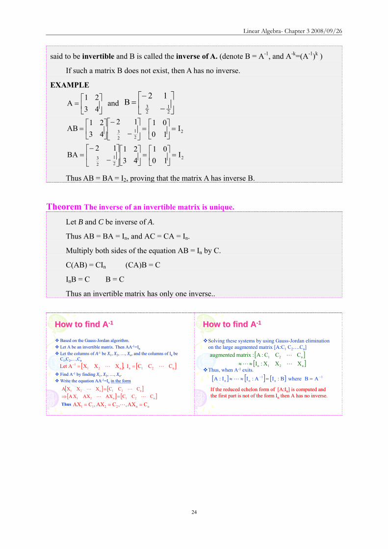
Linear Algebra- Chapter 3 20080926
26
Example Example 1212
Let the message be Let the message be BUY IBM STOCKBUY IBM STOCKAnd the encoding matrix beAnd the encoding matrix be
⎥⎥⎥
⎦
⎤
⎢⎢⎢
⎣
⎡ minusminusminus
434110433
B U Y B U Y -- I B M I B M -- S T O C KS T O C K2 21 25 27 9 2 13 27 19 20 15 3 112 21 25 27 9 2 13 27 19 20 15 3 11
⎥⎥⎥
⎦
⎤
⎢⎢⎢
⎣
⎡ minusminusminusminusminus=
⎥⎥⎥
⎦
⎤
⎢⎢⎢
⎣
⎡
⎥⎥⎥
⎦
⎤
⎢⎢⎢
⎣
⎡ minusminusminus
2331372091431715418461146
222117196116169
27319225271527921112013272
434110433
EncodingEncoding
Example Example 2222
Let the message be Let the message be BUY IBM STOCKBUY IBM STOCKAnd the decoding matrix beAnd the decoding matrix be
⎥⎥⎥
⎦
⎤
⎢⎢⎢
⎣
⎡
minusminus 334344101
B U Y B U Y -- I B M I B M -- S T O C KS T O C K2 21 25 27 9 2 13 27 19 20 15 3 112 21 25 27 9 2 13 27 19 20 15 3 11
⎥⎥⎥
⎦
⎤
⎢⎢⎢
⎣
⎡=
⎥⎥⎥
⎦
⎤
⎢⎢⎢
⎣
⎡ minusminusminusminusminus
⎥⎥⎥
⎦
⎤
⎢⎢⎢
⎣
⎡
minusminus 27319225271527921112013272
2331372091431715418461146
222117196116169
334344101
DecodingDecoding
3-3 Systems of Linear Equations ndash Theoretical Aspects
The system of equations
mnmn22m11m
2nn2222121
1nn1212111
bxaxaxa
bxaxaxabxaxaxa
=+++
=+++=+++
(S)
were aij and bi (1≦i≦m and 1≦j≦n) are scalars in a field F and x1 x2hellipxn are n
variables taking values in F is called a system of m linear equations in n unknows over the
field F
上式稱為佈於 Field F 含有 n 個未知數m 個線性方程式的系統或方程組(system
of m linear equations in n unknows)
The mtimesn matrix
⎟⎟⎟⎟⎟
⎠
⎞
⎜⎜⎜⎜⎜
⎝
⎛
=
mn2m1m
n22221
n11211
aaa
aaaaaa
A is called the coefficient matrix of the
system (S)(係數矩陣) If we let
⎟⎟⎟⎟⎟
⎠
⎞
⎜⎜⎜⎜⎜
⎝
⎛
=
n
2
1
x
xx
x and
⎟⎟⎟⎟⎟
⎠
⎞
⎜⎜⎜⎜⎜
⎝
⎛
=
m
2
1
b
bb
b Then the system (S) may
be rewritten as a single matrix equation Ax = b(單一矩陣方程式)
To exploit the results that we have developed we often consider a system of linear
equations as a single matrix equation
Linear Algebra- Chapter 3 20080926
27
A solution to the system (S) is an n-tuple n
n
2
1
F
s
ss
s isin
⎟⎟⎟⎟⎟
⎠
⎞
⎜⎜⎜⎜⎜
⎝
⎛
= such that As = b The set of
all solutions to the system (S) is called the solution set of the system(解集合) System (S)
is called consistent(相容) if its solution set is nonempty otherwise it is called
inconsistent(不相容)
方程組(S)的解為一 n 序組該序組可以使 As = b方程組的所有解所成的集合
稱為該方程組的解集合(Solution set)方程組的解集合非空集合者稱為「相容」解
集合空集合者稱為「不相容」
EXAMPLE 1
Consider 6x2xx1xx3x2
321
321
=+minus=++
that is ⎟⎟⎠
⎞⎜⎜⎝
⎛=
⎟⎟⎟
⎠
⎞
⎜⎜⎜
⎝
⎛
⎟⎟⎠
⎞⎜⎜⎝
⎛minus 6
1
xxx
211132
3
2
1
(以矩陣表示)
This system has many solutions such as ⎟⎟⎟
⎠
⎞
⎜⎜⎜
⎝
⎛minus=
726
s and ⎟⎟⎟
⎠
⎞
⎜⎜⎜
⎝
⎛
minusminus=
34
8s
Consider 1xx0xx
21
21
=+=+
that is ⎟⎟⎠
⎞⎜⎜⎝
⎛=⎟⎟
⎠
⎞⎜⎜⎝
⎛⎥⎦
⎤⎢⎣
⎡10
xx
1111
2
1
顯然地方程組無解
We begin our study of system of linear equations by examining the class of
homogeneous system of linear equations 先討論齊次方程組
DEFINITION 35 Homogeneous amp Nonhomogeneous
A system Ax=b of m linear equations in n unknowns is said to be homogeneous if b=0
Otherwise the system is said to be nonhomogeneous
方程組 Ax = bb = 0 稱為齊次方程組否則稱為非齊次方程組
Any homogeneous system has at least one solution namely the zero vector The next
result gives further information about the set of solutions to a homogeneous system
Linear Algebra- Chapter 3 20080926
28
齊次方程組至少有一個解那就是『零向量』
Theorem 38 Let Ax = 0 be a homogeneous system of m linear equations in n unknowns over a field
F Let K denote the set of all solutions to Ax = 0 Then K = N(LA) hence K is a subspace
of Fn of dimension n - rank(LA) = n- rank(A)
令 Ax = 0 代表一佈於 Field 含有 n 個未知數m 個線性方程式的方程組若令
K 代表該方程組的解集合(Solution set)則 K = N(LA)K 為 Fn 內的子空間且其維
度為 n ndash rank (LA) = n - rank(A)
【Proof】
Clearly K = sisinFn As = 0 = N(LA) The second part now follows from the
dimension theorem
Nullity(T)+rank(T) = dim(V)
Nullity (LA) = dim (Fn) ndashrank (LA ) = n ndash rank (A)
DEFINTION 27 Let V and W be vector space and let T V W be linear We define
the null space (or kernel) N(T) of T to be the set of all vectors x in V such that T(x) = 0
that is N(T) = xisinV T(x) = 0 V 與 W 為向量空間且 T V W 為線性轉換定義
線性轉換 T 的 Null space 為 V 內所有滿足 T(x) = 0 的向量 x 所形成的集合註記為
N(T)Null space 的元素 x 經線性轉換 T 轉換後所對應的「像」為 0意即 T(x) = 0
Null space 內的元素的「像」皆為 0
DEFINITION 217 Let A be an mtimesn matrix with entries from a field F We denote by LA
the mapping LA Fn Fm defined by LA(x) = Ax (the matrix product A and x) for each
column vector xisinFn We call LA a left-multiplication transformation 令 A 是 mtimesn
的矩陣所有元素均來自 FLA 為 Fn 映至 Fm的線性轉換並定義為 LA(x) = Ax其中
x 為行向量(Column vector)且 xisinFnLA被稱為左乘法轉換
Theorem 23 (Dimension Theorem) Let V and W be vector spaces and let T V W be
linear If V is finite-dimensional then Nullity(T) + rank(T) = dim(V) T 的核次數
(Nullity)與秩(Rank)的和等於定義域的維度 dim(V)
Corollary Let Ax = 0 be a homogeneous system of m linear equations in n unknowns over a field
Linear Algebra- Chapter 3 20080926
29
F If m lt n the system Ax = 0 has a nonzero solution
令 Ax = 0 代表一佈於 Field 含有 n 個未知數m 個線性方程式的方程組若 m
lt n則該方程組具有一非零解
【Proof】
Suppose that m lt n Then rank(A) = rank (LA)≦m Hence dim(K) = n - rank(LA) ≧
n ndash m gt 0 where K = N(LA) Since dim(K) gt 0 Kne 0 Thus there exists a nonzero
vector sisinK so s is a nonzero solution to Ax = 0
設 m lt n則 rank(A) = rank (LA) ≦ m依據 Theorem 38K = sisinFn As = 0
= N(LA) = dim(K) = n - rank(LA) ≧ n ndash m gt 0表示 dim(K) gt 0Kne 0故存在非
零向量 s使得 Ax = 0
EXAMPLE 2
Consider 0xxx
0xx2x
321
321
=minusminus=++
Let ⎟⎟⎠
⎞⎜⎜⎝
⎛minusminus
=111
121A be the coefficient matrix of this system It is clear that rank(A)
= 2 If K is the solution set of this system then dim(K) = 3-2 = 1 Thus any nonzero
solution constitutes a basis for K
若 K 是方程組的解所組成的集合(簡稱為解集合)依 Theorem 38 得知 dim(K)
= 3 - 2 = 1因此任一非零解將形成 K 的基底
For example since ⎟⎟⎟
⎠
⎞
⎜⎜⎜
⎝
⎛minus32
1 is a solution to the given system
⎪⎭
⎪⎬
⎫
⎪⎩
⎪⎨
⎧
⎟⎟⎟
⎠
⎞
⎜⎜⎜
⎝
⎛minus32
1 is a basis for
K Thus any vector in K is of the form ⎟⎟⎟
⎠
⎞
⎜⎜⎜
⎝
⎛minus=
⎟⎟⎟
⎠
⎞
⎜⎜⎜
⎝
⎛minus
t3t2
t
32
1t where tisinR
例如因⎟⎟⎟
⎠
⎞
⎜⎜⎜
⎝
⎛minus32
1是方程組的一個解故
⎪⎭
⎪⎬
⎫
⎪⎩
⎪⎨
⎧
⎟⎟⎟
⎠
⎞
⎜⎜⎜
⎝
⎛minus32
1 為 K 的基底K 內的任一向量均
具有如下形式
⎟⎟⎟
⎠
⎞
⎜⎜⎜
⎝
⎛minus=
⎟⎟⎟
⎠
⎞
⎜⎜⎜
⎝
⎛minus
t3t2
t
32
1t
Linear Algebra- Chapter 3 20080926
30
We now turn to the study of nonhomogeneous systems Our next result shows that the
solution set of a nonhomogeneous system Ax = b can be described in terms of the solution of
the homogeneous system Ax = 0 We refer to the equation Ax = 0 as the homogeneous system
corresponding to Ax = b
以下將進一步探討「非齊次方程組」非齊次方程組 Ax = b 的解集合可利用齊次方
程組 Ax = 0 的解來加以說明因此我們可將 Ax = 0 視為 Ax = b 的齊次方程組
Theorem 39 Let K be the solution set of a system of linear equations Ax = b and let KH be the
solution set of the corresponding homogeneous system Ax = 0 Then for any solution s to
Ax = b K =s + KH = s+k kisinKH
設 K 為線性方程組 Ax = b 的解集合且 KH為對應的齊次方程組的解集合則
對 Ax = b 的任一個解 s 而言K =s + KH = s+k kisinKH
【Proof】
Let s be any solution to Ax = b
We must show that K =s + KH
If wisinK then Aw = b Hence
A(w - s) = Aw ndash As = b ndash b = 0
So w - sisinKH
Thus there exists kisinKH such that w - s = k
It follows that w = s + k isin s +KH and therefore Ksube s +KH
Conversely suppose that wisins +KH then w = s + k for some kisinKH
But then Aw = A(s + k) = As + Ak = b + 0 = b so wisinK
Therefore s +KHsubeK and thus K=s +KH
令 s 為 Ax = b 的任一個解我們必須證明「K =s + KH」
若 wisinK則 Aw = b(即 w 為 Ax = b 的解)
於是 A(w - s) = Aw ndash As = b ndash b = 0
所以 w - sisinKH(即 w-s 為 Ax = 0 的解)
w - s 既然是 KH的元素表示有一元素 kisinKH使得 w - s = kw = s + k
w = s + kisins +KH
Linear Algebra- Chapter 3 20080926
31
因此 Ksube s +KH
反之假設 wisins +KH則 KH中存在一元素 k(kisinKH)使得 w = s + k
因 Aw = A(s + k) = As + Ak = b + 0 = b
故 wisinK 是 Ax = b 的解
因此s +KHsubeK
總結K=s +KH
EXAMPLE 3
Consider 4xxx7xx2x
321
321
minus=minusminus=++
The corresponding homogeneous system is the system in Example 2 It is easily
verified that ⎟⎟⎟
⎠
⎞
⎜⎜⎜
⎝
⎛=
411
s is a solution to the preceeding nonhomogeneous system So the
solution set of the system is ⎪⎭
⎪⎬
⎫
⎪⎩
⎪⎨
⎧isin
⎟⎟⎟
⎠
⎞
⎜⎜⎜
⎝
⎛minus+
⎟⎟⎟
⎠
⎞
⎜⎜⎜
⎝
⎛= Rt
32
1t
411
K by Theorem 39
⎟⎟⎟
⎠
⎞
⎜⎜⎜
⎝
⎛=
411
s 是非齊次方程組 Ax = b 的解
⎟⎟⎟
⎠
⎞
⎜⎜⎜
⎝
⎛minus32
1是齊次方程組的解
依據 Theorem 39 得知線性方程組 Ax = b 的解集合⎪⎭
⎪⎬
⎫
⎪⎩
⎪⎨
⎧isin
⎟⎟⎟
⎠
⎞
⎜⎜⎜
⎝
⎛minus+
⎟⎟⎟
⎠
⎞
⎜⎜⎜
⎝
⎛= Rt
32
1t
411
K
The following theorem will provide us with a means of computing solutions to certain
system of linear equations
Theorem 310~311 提供計算線性方程組的解的方法
Theorem 310 Let Ax = b be a system of n linear equations in n unknowns If A is invertible then the
Linear Algebra- Chapter 3 20080926
32
system has exactly one solution namely A-1b Conversely if the system has exactly one
solution then A is invertible
令 Ax = b 為含 n 個未知數n 個線性方程式的方程組若 A 為可逆則方程組
恰有一個解解為 A-1b反之若該方程組恰有一個解則 A 為可逆
【Proof】
Suppose that A is invertible
Substituting A-1b into system we have A(A-1b)=( AA-1)b = b
Thus A-1b is a solution
If s is an arbitrary solution then As = b
Multiplying both sides by A-1 gives s= A-1b
Thus the system has one and only one solution namely A-1b
假設 A 為可逆將 A-1b 代入方程組可得 A(A-1b)=( AA-1)b = b
故 A-1b 確為方程組的解
若 s 為方程組的任意解則 As = b
兩邊乘上 A-1可得 s= A-1b
因此方程組僅有唯一的解 A-1b
Conversely suppose that the system has exactly one solution s
Let KH denot the solution set for the corresponding homogeneous system Ax = 0
By Theorem 39 s = s + KH But it is so only if KH = 0 Thus N(LA) = 0 and
hence A is invertible
反之假設方程組恰有一個解 s
令 KH為相對應齊次方程組 Ax = 0 的解集合
依據 Theorem 39要能s = s + KH唯有 KH = 0
KH = 0即表示 N(LA) = 0故 A 為可逆
EXAMPLE 4 Consider the following system of three linear equations in three unknowns
1xx3x33x2x4x2
2x4x2
321
321
32
=++=++
=+
In Example 5 of Section 32 we compute the inverse of the coefficient matrix A of
this system Thus the system has exactly one solution namely
Linear Algebra- Chapter 3 20080926
33
⎟⎟⎟
⎠
⎞
⎜⎜⎜
⎝
⎛=
133242420
A⎟⎟⎟
⎠
⎞
⎜⎜⎜
⎝
⎛
+minus+minus+minus+minus+
=minus
41
83
83
21
43
41
43
85
81
1A
⎟⎟⎟
⎠
⎞
⎜⎜⎜
⎝
⎛
minus+minus
=⎟⎟⎟
⎠
⎞
⎜⎜⎜
⎝
⎛
⎟⎟⎟
⎠
⎞
⎜⎜⎜
⎝
⎛
+minus+minus+minus+minus+
==⎟⎟⎟
⎠
⎞
⎜⎜⎜
⎝
⎛minus
814587
41
83
83
21
43
41
43
85
81
1
3
2
1
132
bAxxx
Theorem 311 Let Ax = b be a system of linear equations Then the system is consistent (相容)if
and only if rank(A) = rank (A∣b) Matrix (A b) is called the augmented matrix o∣ f the
system Ax = b
令 Ax = b 為線性方程式方程組則此方程組至少有一個解的『若且唯若』條件
為 rank(A) = rank (A∣b) 矩陣(A∣b)稱為方程組 Ax = b 的增廣矩陣
【Proof】
To say that Ax = b has a solution is equivalent to saying that bisinR(LA)
In the proof of Theorem 35 we saw that R(LA ) = span(a1 a2 an) the span of the
column of A
Thus Ax = b has a solution if and only if bisinspan(a1 a2 an)
But bisinspan(a1 a2 an) if and only if span(a1 a2 an) = span(a1 a2 an b)
This last statement is equivalent to
dim (span(a1a2an)) = dim (span(a1a2an b))
So by Theorem 35 the preceeding equation reduces to rank(A) = rank (A∣b)
Ax = b 有一解相當於 bisinR(LA)即 b 屬於線性轉換 LA的 Range
在 Theorem 35 的證明中提到 R(LA ) = span(a1a2an)aj 為 A 的第 j 個行
(Column)即線性轉換 LA 的 Range 係由矩陣 A 的行(Column)所生成
因此 Ax = b 要有一個解的『若且唯若』條件為 bisinspan(a1 a2 an)
至於 bisinspan(a1 a2 an)之條件
bisinspan(a1a2an) 的『若且唯若』條件為 span(a1a2an) = span(a1a2an
b)
其條件相當於
Linear Algebra- Chapter 3 20080926
34
dim (span(a1a2an)) = dim (span(a1a2an b))
依據 Theorem 35該條件可簡化為 rank(A) = rank (A∣b)
Theorem 35 The rank of any matrix equals the maximum number of its linearly
independent columns that is the rank of a matrix is the dimension of the subspace
generated by its column任一矩陣的 Rank 等於其最大線性獨立行向量數目即矩陣的
Rank 是由矩陣的行向量生成的子空間的維度【LA Fn Fm】
EXAMPLE 5 Recall the system of equations
1xx0xx
21
21
=+=+
Since ⎟⎟⎠
⎞⎜⎜⎝
⎛=
1111
A and ⎟⎟⎠
⎞⎜⎜⎝
⎛=
111011
)bA(
rank(A) = 1 and rank (A b) = 2∣
Because the two ranks are unequal the system has no solutions
矩陣 A 與增廣矩陣(A∣b) 的 Rank 不同故方程組沒有解
EXAMPLE 6 We can use Theorem 311 to determine whether (3 3 2) is in the range of the linear
transformation T R3 R3 defined by T(a1 a2 a3) = (a1+a2+a3 a1-a2+a3 a1+a3)
利用 Theorem 311 來判斷 (3 3 2)是否在線性轉換 T 的 Range 中其中T R3
R3 定義為 T(a1 a2 a3) = (a1+a2+a3 a1-a2+a3 a1+a3)
Now (3 3 2)isinR(T) if and only if there exists a vector s = x1 x2 x3 in R3 such that
T(s)=(3 3 2) Such a vector s must be a solution to the system
2xx3xxx3xxx
31
321
321
=+=+minus=++
Since the ranks of the coefficient matrix and the augmented matrix of this system
are 2 and 3 respectively it follows that this system has no solutions Hence (3 3 2) notin
R(T)
(3 3 2)isinR(T) 的『若且唯若』的條件為存在一向量 s = x1 x2 x3isinR3 使得
T(s)=(3 3 2)
Linear Algebra- Chapter 3 20080926
35
向量 s 必須是 2xx3xxx3xxx
31
321
321
=+=+minus=++
的解
因係數矩陣⎟⎟⎟
⎠
⎞
⎜⎜⎜
⎝
⎛minus
101111111
的 Rank 為 2增廣矩陣⎟⎟⎟
⎠
⎞
⎜⎜⎜
⎝
⎛minus
233
101111111
的 Rank 為 3兩
者不相等故方程組無解(3 3 2) notin R(T)
Theorem 311 Let Ax = b be a system of linear equations Then the system is consistent
(相容)if and only if rank(A) = rank (A∣b) Matrix (A b) is called the ∣ augmented
matrix of the system Ax = b 令 Ax = b 為線性方程式方程組則此方程組至少有一個
解的『若且唯若』條件為 rank(A) = rank (A∣b) 矩陣(A∣b)稱為方程組 Ax = b 的
增廣矩陣
Application
In 1973 Wassily Leontief won the Nobel prize in economics for his work in developing
a mathematical model that can be used to describe various economic phenomena
1973 年Wassily Leontief 因研究一數學模式來描述各種經濟現象而獲頒諾貝爾經
濟獎
CLOSED MODEL
We begin by considering a simple society composed of three peoples (industries) ndash a
farmer who gows all the food a tailor who makes all the clothing and a carpenter who builds
all the housing We assume that each person sells to and buy from a central pool and that
everything produced is consumed Since no commodities either enter or leave the system this
case is referred to as the CLOSE MODEL
考慮一個單純社會的三種人生產食物的農夫製衣的裁縫師與蓋住屋的木匠
並假設採取集中聯營買賣且每一件產品皆付諸消費由於過程中沒有任何成品進入
或脫離這個系統所以稱為「封閉模式」
Each of these three individual consumes all three of the commodities produced in the
Linear Algebra- Chapter 3 20080926
36
society Suppose that the proportion of each of the commodities consumed by each person is
given in the following table
社會中每一位皆消費所生產的三種成品且每一種產品也都被三位所消費其消
費比例如下
食物 Food 衣物 Clothing 住屋 Housing
農夫 Farmer 040 020 020
裁縫師 Tailor 010 070 020
木匠 Carpenter 050 010 060
Let p1 p2 and p3 denote the incomes of the farmer tailor and carpenter respectively To
ensure that this society survives we require that the consumption of each individual equals
his or her income
令 p1p2 與 p3 分別表示農夫裁縫師與木匠的收入並為確保這個封閉社會可以
存活假設每一位的收入等於消費
Note that the farmer consumes 20 of the clothing Because the total cost of all clothing
is p2 the tailorrsquos income the amount spent by the farmer on clothing is 020 p2 Moreover the
amount spent by the farmer on food clothing and housing must equal the farmerrsquos income
and so we obtain the equation 040 p1 + 020 p2 + 030 p3 = p1
對農夫而言農夫的衣物消費佔 20然因所有衣物的消費總額 p2 等於裁縫師的
收入所以農夫在衣物上的消費為 020 p2且農夫在食物衣物與住屋的總消費要等
於農夫的收入 p1所以農夫的收入與消費關係式
040 p1 + 020 p2 + 020 p3 = p1
Similary equations describing the expenditures of the tailor and carpenter produce the
following system of linear equations
同理分別對裁縫師與木匠進行討論可獲得下列方程組
Linear Algebra- Chapter 3 20080926
37
040 p1 + 020 p2 + 020 p3 = p1
010 p1 + 070 p2 + 020 p3 = p2
050 p1 + 010 p2 + 060 p3 = p3
This system can be written as Ap = p
其中⎟⎟⎟
⎠
⎞
⎜⎜⎜
⎝
⎛=
3
2
1
ppp
p 且⎟⎟⎟
⎠
⎞
⎜⎜⎜
⎝
⎛=
600100500200700100200200400
A 稱為輸入-輸出(或消費)矩陣
(Input-output (or consumption) matrix)
Ap = p 稱為均衡條件(Equilibrium condition)
能否利用不等式 p ≦ p 來替代等式
At first it may seem reasonable to replace the equilibrium condition by the inequality
Ap ≦ p that is the requirement that consumption not exceed production But in fact Ap ≦ p implies that Ap = p in the closed model
For otherwise there exists a k for which
sumgt
jjkjk pAp
Hence since the columns of A sum to 1
sumsumsumsum ==gt
jj
i jjij
ii ppAp which is a contradiction (出現矛盾)
答案是在封閉系統中Ap ≦ p Ap = p
One solution to the homogeneous system (I ndash A) x = 0 which is equivalent to the
equilibrium condition is ⎟⎟⎟
⎠
⎞
⎜⎜⎜
⎝
⎛=
400350250
p
Linear Algebra- Chapter 3 20080926
38
齊次方程組(I ndash A) x = 0 或均衡條件的一個解為 ⎟⎟⎟
⎠
⎞
⎜⎜⎜
⎝
⎛=
400350250
p
We may interpret this to mean that the society survives if the farmer taior and carpenter
have incomes in the proportions 253540
⎟⎟⎟
⎠
⎞
⎜⎜⎜
⎝
⎛=
400350250
p 可以解釋為若農夫裁縫師與木匠收入比例為 253540則社會將
能生存下去
Theorem 312
Let A be an ntimesn input-output matrix having the form ⎟⎟⎠
⎞⎜⎜⎝
⎛=
EDCB
A where D is a 1times(n-
1) positive vector and C is an (n-1)times1 positive vector Then (I-A)x = 0 has a one-
dimensional solution set that is generated by a nonnegative vector
設 A 為 ntimesn 輸入-輸出矩陣 ⎟⎟⎠
⎞⎜⎜⎝
⎛=
EDCB
A 其中D 為 1times(n-1)正向量C 為
(n-1)times1 正向量則(I-A)x = 0 具有一維解集合且該解集合係由一非負向量所生成
Any input-output matrix with all positive entries satisfies the hypothesis of this theorem
任何輸入-輸出矩陣滿足 Theorem 312 的基本假設條件例如
⎟⎟⎟
⎠
⎞
⎜⎜⎜
⎝
⎛=
02502503502500650500750
A
OPEN MODEL
In the OPEN MODEL we assume that there is an outside demand for each of the
commodities produced Returning to our simple society let x1 x2 and x3 be the monetary
values of food clothing and housing produced with respective outside demands d1 d2 and d3
Let A be the 3times3 matrix such that Aij represents the amount of commodity i required to
Linear Algebra- Chapter 3 20080926
39
produce one monetary unit of commodity j Then the value of the surplus of food in the
society is x1 ndash (A11x1+A12x2+A13x3) that is the value of food produced minus the value of
food consumed while producing the three commodities The assumption that everything
produced is consumed gives us a similar equilibrium condition for the open model namely
that the surplus of each of the three commodities must equal the corresponding outside
demands Hence i
3
1jjiji dxAx =minussum
=
for j=1 2 3
在「開放模式」中我們假設每一產品皆有外來的需求在前述的單純社會裡
令 x1x2 與 x3 分別代表食物衣物與住屋的貨幣價值d1d2 與 d3 為食物衣物與住
屋的外來需求價值令 A 為 3times3 矩陣Aij 表示生產『一個貨幣單位』的產品 j 所需要
的產品 i 的價值於是此社會中食物的盈餘價值為 x1 ndash (A11x1+A12x2+A13x3)即食物的
價值減去生產食物衣物與住屋所需消耗的食物的價值意即生產出來的食物價值扣
掉用去生產食物衣物與住屋所消耗掉的價值)(A11A12A13 為生產一個貨幣單位
的食物 1衣物 2 與住屋 3 所需消耗的食物 1 數量A12x2 表示生產貨幣價值為 x2的衣物
所需要的食物價值)對每一種產品而言其盈餘價值等於外來的需求價值於是
i
3
1jjiji dxAx =minussum
=
for j=123
Suppose that 30 cents worth of food 10 cents worth of clothing and 30 cents worth of
housing are required for the production of $1 worth of food Similar suppose that 20 cents
worth of food 40 cents worth of clothing and 20 cents worth of housing are required for the
production of $1 worth of clothing Finally suppose that 30 cents worth of food 10 cents
worth of clothing and 30 cents worth of housing are required for the production of $1 worth
of housing Then the input-output matrix is
⎟⎟⎟
⎠
⎞
⎜⎜⎜
⎝
⎛=
300200300100400100300200300
A
假設生產價值 1 元的食物需要價值 30 分的食物(A11 = 03)價值 10 分的衣物
(A21 = 01)及價值 30 分的住屋(A31 = 03)生產價值 1 元的衣物需要價值 20 分的
食物(A12 = 02)價值 40 分的衣物(A22 = 04)及價值 20 分的住屋(A32 = 02)生
Linear Algebra- Chapter 3 20080926
40
產價值 1 元的住屋需要價值 30 分的食物(A13 = 03)價值 10 分的衣物(A23 = 01)
及價值 30 分的住屋(A33 = 03)於是輸入輸出矩陣 A 為
⎟⎟⎟
⎠
⎞
⎜⎜⎜
⎝
⎛=
300200300100400100300200300
A
若食物的外來需求值為 300 億元衣物為 200 億元住屋值為 1 百億元則
⎟⎟⎟
⎠
⎞
⎜⎜⎜
⎝
⎛=
⎟⎟⎟
⎠
⎞
⎜⎜⎜
⎝
⎛
⎟⎟⎟
⎠
⎞
⎜⎜⎜
⎝
⎛
minusminusminusminusminusminus
=minus=
minus
minus
700600900
100200300
700200300100600100300200300
d)AI(x
1
1
⎟⎟⎟
⎠
⎞
⎜⎜⎜
⎝
⎛=
700600900
x 表示要滿足外來需求必須生產的食物價值為 900 億元衣物價值為
600 億元住屋價值為 700 億元
Theorem
Let AX = Y be a system of n linear equations in n variables If Andash1 exists the
solution is unique and is given by X = Andash1Y
【Proof】
Substitute X = Andash1Y into the matrix equation
AX = A(Andash1Y) = (AAndash1)Y = InY = Y
The solution is unique
Let X1 be any solution thus AX1 = Y Multiplying both sides of this equation by Andash1
gives
Andash1AX1= Andash1Y InX1 = Andash1Y X1 = Andash1Y
Linear Algebra- Chapter 3 20080926
41
Example Example 1212
2x5x3x3x5x3x21x2x x
321
321
321
minus=++minus=minusminus=minusminus
⎥⎥⎥
⎦
⎤
⎢⎢⎢
⎣
⎡
minus=
⎥⎥⎥
⎦
⎤
⎢⎢⎢
⎣
⎡
⎥⎥⎥
⎦
⎤
⎢⎢⎢
⎣
⎡
minusminusminusminusminus
231
xxx
531532211
3
2
1
Solve the system of equations
This system can be written in the following matrix form
⎥⎥⎥
⎦
⎤
⎢⎢⎢
⎣
⎡
minus⎥⎥⎥
⎦
⎤
⎢⎢⎢
⎣
⎡
minusminusminusminusminus
=
⎥⎥⎥
⎦
⎤
⎢⎢⎢
⎣
⎡minus
231
531532211
xxx 1
3
2
1
If the matrix of coefficients is invertible the unique solutionIf the matrix of coefficients is invertible the unique solution isis
Example Example 2222
1 2 1 issolution unique The 321 =minus== xxx
⎥⎥⎥
⎦
⎤
⎢⎢⎢
⎣
⎡minus=
⎥⎥⎥
⎦
⎤
⎢⎢⎢
⎣
⎡
minus⎥⎥⎥
⎦
⎤
⎢⎢⎢
⎣
⎡
minusminusminus=
⎥⎥⎥
⎦
⎤
⎢⎢⎢
⎣
⎡
121
231
123135110
xxx
3
2
1
⎥⎥⎥
⎦
⎤
⎢⎢⎢
⎣
⎡
minusminusminus=
⎥⎥⎥
⎦
⎤
⎢⎢⎢
⎣
⎡
minusminusminusminusminus
=
minus
minus
123135110
531532211
A
1
1
The The LeontiefLeontief IO Model in IO Model in Economics Economics 1515
The Leontief input-output model is used to analyze the interdependence of economics Wassily Leontief received a Nobel Prize in 1973 for his work in thie fieldThe practical applications of this model have proliferated until it has now become a standard tool for investigating economic structures ranging from cities and corporation to states and countriesConsider an economics situation that involves ninterdependent industries The output of any one industry is needed as input by other industries and even possibly by the industry itself
The The LeontiefLeontief IO Model in IO Model in Economics Economics 2525
How a mathematical model involving a system of linear equations can be constructed to analyze such a situationAssume that each industry produces one commodity Let aij denote the amount of input of a certain commodity i to produce unit output of commodity j In our model let the amounts of input and output be measured in dollars Thus for example a34 = 045 means that 45 centsrsquo worth of commodity 3 is required to produce one dollarrsquos worth of commodity 4
The The LeontiefLeontief IO Model in IO Model in Economics Economics 3535
aij = amount of commodity i in one dollar of commodity jaij =生產一元價值的j產品需要耗用的i產品價值
The elements aij called input coefficients define a matrix A called the input-output matrix which describes the interdependence of the industriesExtending the model to include an open sector (all non-producing sectors) The product of industries may go not only into other producing industries but also into other non-producing sectors of the economy such as consumers and governments
The The LeontiefLeontief IO Model in IO Model in Economics Economics 4545
di = demand of the open sectors from industry ixi=total output of industry I necessary to meet demands of all n industries and the open sector
sectoropen of demand
nindustry of demand
2industry of demand
22
1industry of demand
11
industry ofoutput total
ininii
i
i dxaxaxax ++sdotsdotsdot++=
output ofportion sectoropen
output ofportion tryinterindusoutput total
DAXX +=Demand matrixDemand matrix
Output matrixOutput matrix
The The LeontiefLeontief IO Model in IO Model in Economics Economics 5555
Applying the model to the economy of a country X Applying the model to the economy of a country X represents the total output of each of the producing sectors represents the total output of each of the producing sectors of the economy and AX describes the contributions made of the economy and AX describes the contributions made by the various sectors to fulfilling the intersectional input by the various sectors to fulfilling the intersectional input requirements of the economyrequirements of the economyD is equal to (XD is equal to (X--AX) the difference between total output AX) the difference between total output X and industry transaction AXX and industry transaction AXD is thus the gross national product of the economyD is thus the gross national product of the economy
Example Example 1414
Consider an economy consisting of three industries having Consider an economy consisting of three industries having the following inputthe following input--output matrix output matrix AA Determine the output Determine the output levels required of the industries to meet the demands of levels required of the industries to meet the demands of the other industries and of the open sector in each casethe other industries and of the open sector in each case
in turn 321812
and 896
1612
9
5100
021
21
103
51
51
⎥⎥⎦
⎤
⎢⎢⎣
⎡
⎥⎥⎦
⎤
⎢⎢⎣
⎡
⎥⎥⎦
⎤
⎢⎢⎣
⎡=
⎥⎥⎥
⎦
⎤
⎢⎢⎢
⎣
⎡
= DA
The unit of The unit of DD are millions of dollarsare millions of dollars
Linear Algebra- Chapter 3 20080926
42
Example Example 2424
We wish to compute the output levels X that correspond to We wish to compute the output levels X that correspond to the various open sector demands D X is given by the the various open sector demands D X is given by the equation X = AX + D Rewritten as followsequation X = AX + D Rewritten as follows
X ndash AX = D rArr (I ndash A)X = D rArr X = (I ndash A) ndash1 D
⎥⎥⎥
⎦
⎤
⎢⎢⎢
⎣
⎡
=⎥⎥⎥
⎦
⎤
⎢⎢⎢
⎣
⎡
minus⎥⎥⎦
⎤
⎢⎢⎣
⎡=minus minus
minusminus
5400
021
21
103
51
54
5100
021
21
103
51
31
100010001
get We AI
⎥⎥⎥
⎦
⎤
⎢⎢⎢
⎣
⎡
=minus minus
4500
038
35
85
32
35
1)( AI
output ofingcorrespond valuesvarious
4500
038
35
85
32
35
)(
401020883957522133
32816189121269
)(
1
1
DAI
DAIX
minus
minus
minusuarruarruarruarruarruarruarr
⎥⎥⎦
⎤
⎢⎢⎣
⎡=
⎥⎥⎦
⎤
⎢⎢⎣
⎡
⎥⎥⎥
⎦
⎤
⎢⎢⎢
⎣
⎡
=minus=
Example Example 3434
By using Gauss-Jordan elimination
dollars of milliond are units The
40
15674
and 106629
209946
are 321812
and 896
1612
9
⎥⎥⎥
⎦
⎤
⎢⎢⎢
⎣
⎡
⎥⎥⎥
⎦
⎤
⎢⎢⎢
⎣
⎡
⎥⎥⎥
⎦
⎤
⎢⎢⎢
⎣
⎡
⎥⎥⎥
⎦
⎤
⎢⎢⎢
⎣
⎡
⎥⎥⎥
⎦
⎤
⎢⎢⎢
⎣
⎡
⎥⎥⎥
⎦
⎤
⎢⎢⎢
⎣
⎡
Example Example 4444
The output levels necessary to meet the demandsThe output levels necessary to meet the demands
IAAAIAI m =++++minus ))(( 2 L
mAAAIAI ++++=minus minus L21)(
Computing (IComputing (I--A) A) --11
1m
m2m2
m2
AI)AAAI(A)AAAI(I
)AAAI)(AI(
+minus=++++minus++++=
++++minusLL
L
NOTE 0A 1m rarr+
Population Movement Population Movement 1313
In 2000 58 million of people live in cities and 142 million of In 2000 58 million of people live in cities and 142 million of people people live in the surrounding suburbs Represent this information by tlive in the surrounding suburbs Represent this information by the he matrix matrix
The probability of a person staying in the city was 096 Thus tThe probability of a person staying in the city was 096 Thus the he probability of moving to the suburbs was 004 probability of moving to the suburbs was 004 The probability of a person moving to the city was 001 the The probability of a person moving to the city was 001 the probability of remaining in suburbia was 099probability of remaining in suburbia was 099
suburbcity
990040010960
suburbcity (to))from(
⎥⎦
⎤⎢⎣
⎡=P
⎥⎦
⎤⎢⎣
⎡=
14258
X0
City population in 2001 = people who remained from 2000 + peopleCity population in 2001 = people who remained from 2000 + peoplewho moved in from the suburbs = ( 096 who moved in from the suburbs = ( 096 timestimes 58 ) + (001 58 ) + (001 timestimes 142 ) = 142 ) = 571 million571 millionSuburban population in 2001 = people who moved in from the city Suburban population in 2001 = people who moved in from the city + people who stayed from 2000 = ( 004 + people who stayed from 2000 = ( 004 timestimes 58 ) + (099 58 ) + (099 timestimes 142 ) = 142 ) = 1429 million1429 millionCan arrive at these numbers using matrix multiplicationCan arrive at these numbers using matrix multiplication
⎥⎦
⎤⎢⎣
⎡=⎥
⎦
⎤⎢⎣
⎡⎥⎦
⎤⎢⎣
⎡==
9142157
14258
990040010960
PXX 01
Population Movement Population Movement 2323
Population Movement Population Movement 3333
Assume that the population flow represented by the matrix P is unchanged over the years The population distribution X2 after 2 years is given by X2 = P X1 = P2 X0 In general
Pn is called the n-step transition matrix The (ij)th element of Pngives the probability of going from state j to state i in n stepsFor example
in
ni XPX =+
suburbcity
960150040850
P
suburbcity (to))from(
4
⎥⎦
⎤⎢⎣
⎡=
The probability of living in the city in The probability of living in the city in 2000 and being in the suburbs 4 years 2000 and being in the suburbs 4 years later is 015later is 015
Markov ChainsMarkov Chains
The probabilities in the above model depend only on the The probabilities in the above model depend only on the current state of a person whether the person is living in the current state of a person whether the person is living in the city or in suburbiacity or in suburbiaThis type of model in which the probability of going from This type of model in which the probability of going from one state to another depends only on the current state one state to another depends only on the current state rather than on a more complete historical description is rather than on a more complete historical description is called a called a Markov chainMarkov chainMarkov chains are useful tools for scientists in many Markov chains are useful tools for scientists in many fields such as geneticsfields such as genetics
Linear Algebra- Chapter 3 20080926
43
GeneticsGenetics 1414
Genetics is the branch of biology that deals with Genetics is the branch of biology that deals with heredity heredity (遺傳)(遺傳) It is the study of units called It is the study of units called genes which determine the characteristics living genes which determine the characteristics living things inherit from their parents The inheritance things inherit from their parents The inheritance (遺傳)(遺傳)of such traitsof such traits(特徵)(特徵)as sex height eye as sex height eye color and hair color of human beings and such color and hair color of human beings and such traits as petaltraits as petal(花瓣)(花瓣) color and leaf shape of color and leaf shape of plants are governed by genesplants are governed by genesIn medicine agricultureIn medicine agriculturehelliphellip
GeneticsGenetics 2424
The traits of guinea pigsThe traits of guinea pigs(天竺鼠)(天竺鼠)are long hair and short hairare long hair and short hairThe length of hair is governed by a pair of gene which we denoteThe length of hair is governed by a pair of gene which we denote A A and aand aA guinea pig may have any one of the combination of AA A guinea pig may have any one of the combination of AA AaAa or or aaaa Each of these classes is called a genotypeEach of these classes is called a genotype(基因型)(基因型)The AA type guinea pig is indistinguishable in appearance from tThe AA type guinea pig is indistinguishable in appearance from the he AaAa type type ndashndash both have long hair both have long hair ndashndash whereas the whereas the aaaa type has short hairtype has short hairThe A gene is said to dominate the a geneThe A gene is said to dominate the a geneAn animal is called dominant An animal is called dominant (顯性)(顯性)if it has AA genes hybridif it has AA genes hybrid(混種)(混種) with with AaAa genes and recessive genes and recessive (隱性)(隱性)with with aaaa genesgenes
GeneticsGenetics 3434
When two guinea pigs are crossed the offspring inherits one genWhen two guinea pigs are crossed the offspring inherits one gene e from each parent in random mannerfrom each parent in random mannerGiven the genotype of the parents we can determine the Given the genotype of the parents we can determine the probabilities of the genotype of the offspringprobabilities of the genotype of the offspring
AA+AA AA+AA probabilities of AA probabilities of AA AaAa and and aaaa are 10and 0are 10and 0Aa+AAAa+AA probabilities of AA probabilities of AA AaAa and and aaaa are are frac12frac12 frac12frac12 and 0 and 0aa+AAaa+AA probabilities of AA probabilities of AA AaAa and and aaaa are 0 1 and 0are 0 1 and 0
This series of experiments is a Markov chain having transition This series of experiments is a Markov chain having transition matrixmatrix
aaAaAA
00012100211
P
aaAaAA
⎥⎥⎥
⎦
⎤
⎢⎢⎢
⎣
⎡=
GeneticsGenetics 4444
Assume an initial population of guinea pigs made up of an Assume an initial population of guinea pigs made up of an equal number of each genotypeequal number of each genotype
⎥⎥⎥
⎦
⎤
⎢⎢⎢
⎣
⎡=
313131
X0
The fractions of following generations are
⎥⎥⎥
⎦
⎤
⎢⎢⎢
⎣
⎡=
⎥⎥⎥
⎦
⎤
⎢⎢⎢
⎣
⎡=
⎥⎥⎥
⎦
⎤
⎢⎢⎢
⎣
⎡=
⎥⎥⎥
⎦
⎤
⎢⎢⎢
⎣
⎡=
01611615
X08187
X04143
X02121
X 4321
AAAAAaAaaaaa
3-4 Systems of Linear Equations ndash Computational Aspects
DEFINITION 36 Equivalent
Two systems of linear equations are called equivalent if they have the same solution
set
兩個線性方程組稱為等價意指兩者具有相同的解集合
Elementary Transformations Transformation called elementary transformations can be used to change a system of
linear equations into another system of linear equations that have the same solution
These transformations are used to solve system of linear equations by eliminating
variables
The equivalent transformations used in terms of matrix are called ELEMENTARY
ROW OPERATION
Linear Algebra- Chapter 3 20080926
44
Equivalent System Systems of equations that are related through elementary transformations are called
equivalent systems
Matrices that are related through elementary row operations are called row equivalent
matrices
The symbol asymp is used to indicate equivalence in both cases
Theorem 313 Let Ax = b be a system of m linear equations in n unknowns and let C be an invertible
mtimesm matrix Then the system (CA)x = Cb is equivalent to Ax = b
設 Ax = b 為含 n 個未知數m 個線性方程式的方程組若 C 為可逆的mtimesm
矩陣則(CA)x = Cb 等價於 Ax = b
【Proof】
Let K be the solution set for Ax = b and Krsquo the solution set for (CA)x = Cb If wisinK
then Aw = b So (CA)w = Cb and hence wisinKrsquo Thus KsubeKrsquo
Conversely if wisinKrsquo then (CA)w = Cb Hence Aw = C-1(CA)w = C-1(Cb) = b so
wisinK Thus KrsquosubeK and therefore K=Krsquo
設 K 為 Ax = b 的解集合且 Krsquo為(CA)x = Cb 的解集合
若 wisinK則 Aw = b (CA)w = Cb故 wisinKrsquo於是 KsubeKrsquo
反之若 wisinKrsquo則(CA)w = Cb Aw = C-1(CA)w = C-1(Cb) = b故 wisinK於是
KrsquosubeK因此K=Krsquo
Corollary Let Ax = b be a system of m linear equations in n unknowns If (Arsquo brsquo) is obtained ∣
from from (A b) by a finite number of elementary row operations then the system Arsquox = ∣
brsquo is equivalent to the original system
設 Ax = b 為含 n 個未知數m 個線性方程式的方程組若(Arsquo brsquo) ∣ 是由(A b) ∣
經過有限次數的基本列運算而得則 Arsquox = brsquo 等價於 Ax = b即兩者具有相同的解
集合
【Proof】
Suppose that (Arsquo brsquo) is obtained from (A b) by elementary row operations These ∣ ∣
Linear Algebra- Chapter 3 20080926
45
may be executed by multiplying (A b) by elementary mtimesm matrices E∣ 1 E2hellipEp Let
C=EphellipE2E1 then (Arsquo brsquo) = C(A b) = (CA Cb)∣ ∣ ∣
Since each Ei is invertible so is C Now Arsquo = CA and brsquo = Cb Thus by Theorem 313
the system Arsquox = brsquo is equivalent to the system Ax = b
設(Arsquo brsquo)∣ 是由(A b)∣ 經過基本列運算取得即以基本 mtimesm 矩陣 E1 E2hellipEp
乘上 (A b)∣ (Arsquo brsquo) = C(A b) = (CA Cb∣ ∣ ∣ )其中C=EphellipE2E1
因 Ei 可逆故 C 亦為可逆 Arsquo = CA 且 brsquo = Cb
依據 Theorem 313Arsquox = brsquo 等價於 Ax = b
Theorem 313 Let Ax = b be a system of m linear equations in n unknowns and let C be an
invertible mtimesm matrix Then the system (CA)x = Cb is equivalent to Ax = b 設 Ax = b
為含 n 個未知數m 個線性方程式的方程組若 C 為可逆的mtimesm 矩陣則(CA)x
= Cb 等價於 Ax = b
We now describe a method for solving any stystem of linear equations Consider for
example the system of linear equations
探討解線性方程組的方法hellip
2xxx2x3xxx1x2x3x2x3
4321
321
4321
=minus++=++=minus++
First we form the augmented matrix ⎟⎟⎟
⎠
⎞
⎜⎜⎜
⎝
⎛
minus
minus
231
112101112323
(增廣矩陣)
Interchanging the first and third rows ⎟⎟⎟
⎠
⎞
⎜⎜⎜
⎝
⎛
minus
minus
132
132301111121
(第 13 列互調)
Adding -1 times the first row to the second row and then add -3 times the first row to
the third row ⎟⎟⎟
⎠
⎞
⎜⎜⎜
⎝
⎛
minusminusminus
minus
512
104010101121
(第 1 列乘上 -1 加到第 2 列再以 -3 乘上
第 1 列加到第 3 列)
Linear Algebra- Chapter 3 20080926
46
Multiplying the second row by -1 ⎟⎟⎟
⎠
⎞
⎜⎜⎜
⎝
⎛
minusminus
minusminusminus
51
2
104010101121
(第 2 列乘上 -1)
Adding four times the second row to the third row ⎟⎟⎟
⎠
⎞
⎜⎜⎜
⎝
⎛
minusminus
minusminusminus
91
2
300010101121
(4 乘上第 2
列加到第 3 列)
Multiplying the third row by -13 ⎟⎟⎟
⎠
⎞
⎜⎜⎜
⎝
⎛minusminus
minus
31
2
100010101121
(第 3 列乘上 -13)
Adding the third row to the first and second rows to obtain zeros in row 1 column 4
and row 2 column 4 ⎟⎟⎟
⎠
⎞
⎜⎜⎜
⎝
⎛
325
100000100121
(將第 3 列加到第 1 列及第 2 列)
Adding -2 times the second row to the first row in order to make the first row second
column entry become zero ⎟⎟⎟
⎠
⎞
⎜⎜⎜
⎝
⎛
321
100000100101
(將第 2 列乘以 -2 再加至第 1 列)
We have now obtained the desired reduction of the augmented matrix
⎟⎟⎟
⎠
⎞
⎜⎜⎜
⎝
⎛
321
100000100101
是化簡後的增廣矩陣
This matrix corresponds to the system of linear equations
對應的線性方程組為
2x3x1xx
4
2
31
===+
By Corollary to Theorem 313 this system is equivalent to the original system But this
system is easily solved Obviously x2 = 2 and x4 = 3 Moreover x1 and x3 can be any values
Linear Algebra- Chapter 3 20080926
47
provided their sum is 1 Letting x3 = t we then have x1 = 1 ndash t Thus an arbitray solution to the
original system has the form
依據 Corollary to Theorem 313 化簡後的方程組與原方程組等值此方程組的解為
x2 = 3x4 = 3x1 + x3 = 1於是原方程組的任意解可以寫成
⎟⎟⎟⎟⎟
⎠
⎞
⎜⎜⎜⎜⎜
⎝
⎛minus
+
⎟⎟⎟⎟⎟
⎠
⎞
⎜⎜⎜⎜⎜
⎝
⎛
=
⎟⎟⎟⎟⎟
⎠
⎞
⎜⎜⎜⎜⎜
⎝
⎛ minus
0101
t
3021
3t2
t1
Observe that
⎪⎪⎭
⎪⎪⎬
⎫
⎪⎪⎩
⎪⎪⎨
⎧
⎟⎟⎟⎟⎟
⎠
⎞
⎜⎜⎜⎜⎜
⎝
⎛minus
0101
is a basis for the homogeneous system of equations
corresponding to the given system
其中
⎪⎪⎭
⎪⎪⎬
⎫
⎪⎪⎩
⎪⎪⎨
⎧
⎟⎟⎟⎟⎟
⎠
⎞
⎜⎜⎜⎜⎜
⎝
⎛minus
0101
是齊次方程組解集合的一組基底
Gauss-Jordan Elimination
Let A be an n times n matrix
1 Adjoin the identity n times n matrix In to A to form the matrix [A In]
2 Compute the reduced echelon form of [A In]
(1) If the reduced echelon form is of the type [In B] then B is the inverse of A
(2) If the reduced echelon form is not of the type [In B] in that the first n times n
submatrix is not In then A has no inverse
An n times n matrix A is invertible if and only if its reduced echelon form is In
DEFINITION 37 Reduced Row Echelon Form
A matrix is said to be in reduced row echelon form if the following three conditions
are satisfied
Linear Algebra- Chapter 3 20080926
48
一個矩陣可以被稱為簡約列梯形式必須具備有下列三條件
(a) Any row containing a nonzero entry preceeds any row in which all the entries are
zero (if any)
含有非零元素的任一列排在全含零元素的任一列前面(儘可能)
(b) The first nonzero entry in each row in the only nonzero entry in its column
各列中第一個非零元素為其所在行中唯一的非零元素
(c) The first nonzero entry in each row is 1 and it occurs in a column to thr right of the
first nonzero entry in the preceeding row
各列中第一個非零元素為 1 且它出現在前一列中第一個非零元素的右邊某一
行中
Reduced Echelon Form A matrix is in reduced echelon form if
1 Any rows consisting entirely of zeros are grouped at the bottom of the matrix
2 The first nonzero element of each other row is 1 This element is called a leading 1
3 The leading 1 of each row after the first is positioned to the right of the leading 1 of
the previous row
4 All other elements in a column that contains a leading 1 are zero
Theorem 314 Gaussian Elimination Transformation Gaussian elimination transform any matrix into its reduced row echelon form
利用 Gaussian elimination 將矩陣轉換成簡約列梯形式
We now describe a method for solving a system in which the augmented matrix is in
reduced row echelon form To illustrate this procedure we consider the system
14x8x3x2x2x28x5x2xxx6x3xxxx17x9x4xx3x2
54321
54321
54321
54321
=minus+++=minus+++=minus+++=minus+++
Linear Algebra- Chapter 3 20080926
49
for which the augmented matrix is
⎟⎟⎟⎟⎟
⎠
⎞
⎜⎜⎜⎜⎜
⎝
⎛
minusminusminusminus
1486
17
83222521113111194132
(增廣矩陣)
Applying Gaussian elimination to the augmented matrix of the system produces the
following sequence of matrices
利用 Gaussian elimination method 處理增廣矩陣
⎟⎟⎟⎟⎟
⎠
⎞
⎜⎜⎜⎜⎜
⎝
⎛
minusminusminusminus
1486
17
83222521113111194132
⎟⎟⎟⎟⎟
⎠
⎞
⎜⎜⎜⎜⎜
⎝
⎛
minusminusminusminus
148
176
83222521119413231111
⎟⎟⎟⎟⎟
⎠
⎞
⎜⎜⎜⎜⎜
⎝
⎛
minusminus
minus
0213
0000021000
1011020201
The system of linear equations corresponding to thus last matrix is
對應最後矩陣的線性方程組 2x2x
1xxx3x2x2x
54
532
531
=minus=+minus=minus+
Assign x3 = t1 x5 = t2
2t22x2x1tt1xxx
3t2t23x2x2x
254
21532
21531
+=+=+minus=+minus=
++minus=++minus=
Thus an arbitray solution s is of the form
於是任意解 s 具有下列形式
s =
⎟⎟⎟⎟⎟⎟
⎠
⎞
⎜⎜⎜⎜⎜⎜
⎝
⎛minus
+
⎟⎟⎟⎟⎟⎟
⎠
⎞
⎜⎜⎜⎜⎜⎜
⎝
⎛minus
+
⎟⎟⎟⎟⎟⎟
⎠
⎞
⎜⎜⎜⎜⎜⎜
⎝
⎛
=
⎟⎟⎟⎟⎟⎟
⎠
⎞
⎜⎜⎜⎜⎜⎜
⎝
⎛
+
+minus++minus
=
⎟⎟⎟⎟⎟⎟
⎠
⎞
⎜⎜⎜⎜⎜⎜
⎝
⎛
1201
2
t
00112
t
02013
t2t2
t1tt
3t2t2
xxxxx
21
2
2
1
21
21
5
4
3
2
1
where t1t2isinR
Linear Algebra- Chapter 3 20080926
50
Notice that
⎪⎪⎪
⎭
⎪⎪⎪
⎬
⎫
⎪⎪⎪
⎩
⎪⎪⎪
⎨
⎧
⎟⎟⎟⎟⎟⎟
⎠
⎞
⎜⎜⎜⎜⎜⎜
⎝
⎛minus
⎟⎟⎟⎟⎟⎟
⎠
⎞
⎜⎜⎜⎜⎜⎜
⎝
⎛minus
1201
2
00112
is a basis for the solution set of the corresponding
homogeneous system of equation and
⎟⎟⎟⎟⎟⎟
⎠
⎞
⎜⎜⎜⎜⎜⎜
⎝
⎛
02013
is a particular solution to the original system
⎪⎪⎪
⎭
⎪⎪⎪
⎬
⎫
⎪⎪⎪
⎩
⎪⎪⎪
⎨
⎧
⎟⎟⎟⎟⎟⎟
⎠
⎞
⎜⎜⎜⎜⎜⎜
⎝
⎛minus
⎟⎟⎟⎟⎟⎟
⎠
⎞
⎜⎜⎜⎜⎜⎜
⎝
⎛minus
1201
2
00112
是齊次方程組解集合的一組基底
⎟⎟⎟⎟⎟⎟
⎠
⎞
⎜⎜⎜⎜⎜⎜
⎝
⎛
02013
是原方程組的特別解
EXAMPLE 1
The matrix ⎟⎟⎟
⎠
⎞
⎜⎜⎜
⎝
⎛
101010011
is not in reduced row echelon form
因為第一行含有第一個非零元素在第一列但第一行尚含有其他非零元素
The matrix ⎟⎟⎟
⎠
⎞
⎜⎜⎜
⎝
⎛
110010012010
is not in reduced row echelon form
因為第一列第一個非零元素不在第一列第一個非零元素的右邊
The matrix ⎟⎟⎠
⎞⎜⎜⎝
⎛010002
is not in reduced row echelon form
因為第一列的第一個非零元素不是 1
Linear Algebra- Chapter 3 20080926
51
Reduced Echelon FormReduced Echelon Form
⎥⎥⎥
⎦
⎤
⎢⎢⎢
⎣
⎡
910030107001
⎥⎥⎥
⎦
⎤
⎢⎢⎢
⎣
⎡
100001000041
⎥⎥⎥
⎦
⎤
⎢⎢⎢
⎣
⎡
000210801
Not in Reduced Echelon Form
⎥⎥⎥
⎦
⎤
⎢⎢⎢
⎣
⎡
310000004021
⎥⎥⎥
⎦
⎤
⎢⎢⎢
⎣
⎡
100000430003021
⎥⎥⎥⎥
⎦
⎤
⎢⎢⎢⎢
⎣
⎡
0000210030108071
In Reduced Echelon Form
Use GaussUse Gauss--Jordan elimination to Jordan elimination to find reduced echelon formfind reduced echelon form 1313
Step 1 Interchange rows if necessary to bring a nonzero Step 1 Interchange rows if necessary to bring a nonzero element to the top of the first nonzero column This nonzero element to the top of the first nonzero column This nonzero element is called a pivotelement is called a pivot
⎥⎥⎦
⎤
⎢⎢⎣
⎡
minusminus
minus
1211244129333
22200
⎥⎥⎥
⎦
⎤
⎢⎢⎢
⎣
⎡
minusminus
minus
harrasymp
121124422200
129333
R2R1
Use GaussUse Gauss--Jordan elimination to Jordan elimination to find reduced echelon formfind reduced echelon form 2323
Step 2 Create a 1 in the pivot location by multiplying the Step 2 Create a 1 in the pivot location by multiplying the pivot row by 1pivotpivot row by 1pivot
Step 3 Create zero elsewhere in the pivot column by adding Step 3 Create zero elsewhere in the pivot column by adding suitable multiples of the pivot row to all other rows of the suitable multiples of the pivot row to all other rows of the matrixmatrix
⎥⎥⎥
⎦
⎤
⎢⎢⎢
⎣
⎡
minusminusminus
minus
minus+asymp
412002220043111
4)R1(R3
⎥⎥⎦
⎤
⎢⎢⎣
⎡
minusminus
minus
⎟⎠⎞
⎜⎝⎛asymp
12112442220043111
R13
1
The matrix is the reduced echelon form of the given matrixThe matrix is the reduced echelon form of the given matrix
Use GaussUse Gauss--Jordan elimination to Jordan elimination to find reduced echelon formfind reduced echelon form 3333
Step 4 Cover the pivot row and all rows above it Repeat Steps Step 4 Cover the pivot row and all rows above it Repeat Steps 1 1 and 2 for the remaining and 2 for the remaining submatrixsubmatrix Repeat Step 3 for the whole Repeat Step 3 for the whole matrix Continue until the reduced echelon form is reachedmatrix Continue until the reduced echelon form is reached
⎥⎥⎥
⎦
⎤
⎢⎢⎢
⎣
⎡
minusminus
+minus+asymp
⎥⎥⎥
⎦
⎤
⎢⎢⎢
⎣
⎡
minusminus
minus++asymp
⎥⎥⎥
⎦
⎤
⎢⎢⎢
⎣
⎡
minusminusminus
minus
⎟⎠⎞
⎜⎝⎛
asymp
⎥⎥⎥
⎦
⎤
⎢⎢⎢
⎣
⎡
minusminusminus
minus
6100050100
170011
R3R22)R3(R1
610001110052011
R2)2(R3R2R1
412001110043111
R221
412002220043111
Theorem 315 Let Ax = b be a system of r nonzero equations is in n unknown Suppose that rank(A)
= rank (A b)∣ and that (A b)∣ is in reduced row echelon form Then
設 Ax = b 為含有 n 個未知數r 個非零方程式的方程組假設 rank(A) = rank
(A b)∣ 且 (A b)∣ 為簡約列梯形式於是
(a) rank(A) = r
(b) If the general solution obtained by the procedure above is of the form s = s0 + t1u1
+ t2u2 +hellip+ tn-run-r then u1 u2hellip un-r is a basis for the solution set of the
corresponding homogeneous system and s0 is a solution to the original system 由
前述方法所得的 General solution 具有下列形式
s = s0 + t1u1 + t2u2 +hellip+ tn-run-r
其中u1 u2hellip un-r為齊次方程組 Ax = 0 的解集合的一組基底且 s0 為原方
程組的一個解)
【Proof】
Since (A b)∣ is in reduced row echelon form (A b)∣ must have r nonzero rows
Clearly these rows are linearly independent by the definition of the reduced row echelon
Linear Algebra- Chapter 3 20080926
52
form and so rank (A b)∣ = r Thus rank(A) = r
Let K be the solution set for Ax = b and let KH be the solution set for Ax = 0 Setting
t1 = t2 =hellip= tn-r = 0 we see that s = s0isinK But by Theorem 39 K = s +KH Hence
KH = - s0+K = span(u1 u2hellip un-r )
Because rank(A) = r we have dim(KH) = n-r Thus since dim(KH) = n-r and KH is
generated by a set u1 u2hellip un-r containing at most n-r vectors that is a basis for KH
由於(A b)∣ 具有簡約列梯形式因此(A b)∣ 必定具有 r 個非零列由簡約列梯形
式的定義得知 r 個非零列為線性獨立故 rank (A b)∣ = rrank(A) = r
令 K 為 Ax = b 的解集合 KH 為 Ax = 0 的解集合
假設 t1 = t2 =hellip= tn-r = 0(u1 u2hellip un-r非 KH的基底)則 s = s0isinK
依據 Theorem 39K = s +KH KH = - s0+K = span(u1 u2hellip un-r )
因 rank(A) = r所以 dim(KH) = n - r 且 KH 是由u1 u2hellip un-r 所生成
故原假設「t1 = t2 =hellip= tn-r = 0」不成立
因此 KH含有最多 n - r 個向量且這些向量為 KH的基底
Theorem 39 Let K be the solution set of a system of linear equations Ax = b and let KH be
the solution set of the corresponding homogeneous system Ax = 0 Then for any solution s
to Ax = b K =s + KH = s+k kisinKH 設 K 為線性方程組 Ax = b 的解集合且 KH
為對應的齊次方程組的解集合則對 Ax = b 的任一個解 s 而言K =s + KH = s+k
kisinKH
ExampleExampleSolve the system of equationsSolve the system of equations
7537429333
321
321
321
=minusminus=+minus=+minus
xxxxxxxxx
⎥⎥⎦
⎤
⎢⎢⎣
⎡
++asymp
000012104301
R2R3R2R1 12
431243
32
31
32
31+minus=+minus=rArr=+
=+rArr xxxx
xxxx
The general solution to the system isThe general solution to the system is
parameter) a (callednumber real is where 1243
3
2
1
rrxrxrx
=+minus=+minus=
⎥⎥⎥
⎦
⎤
⎢⎢⎢
⎣
⎡
minusminusminus
minus
minus+minus+asymp
⎥⎥⎥
⎦
⎤
⎢⎢⎢
⎣
⎡
minusminusminusminus
asymp
⎥⎥⎥
⎦
⎤
⎢⎢⎢
⎣
⎡
minusminusminusminus
242012103111
1R)3(3R1R)2(2R
715374123111
715374129333
R131
ExampleExample
Solve the system of equationsSolve the system of equations446942
1423258101242
4321
4321
4321
=minus+minusminus=+minus+minus
=minus+minus
xxxxxxxxxxxx
⎪⎪
⎩
⎪⎪
⎨
⎧
===
minus=
rArr==minus=minus
rArr
1x6xrx
2r2x
1x6x
2x2x
4
3
2
1
4
3
21
⎥⎥⎥
⎦
⎤
⎢⎢⎢
⎣
⎡ minusminusasymp
⎥⎥⎥
⎦
⎤
⎢⎢⎢
⎣
⎡minus
minusminusasymp
⎥⎥⎥
⎦
⎤
⎢⎢⎢
⎣
⎡
minusminusminusminusminusasymp
⎥⎥⎥
⎦
⎤
⎢⎢⎢
⎣
⎡
minusminusminusminusminusasymp
⎥⎥⎥
⎦
⎤
⎢⎢⎢
⎣
⎡
minusminusminusminusminus
minusminusasymp
⎥⎥⎥
⎦
⎤
⎢⎢⎢
⎣
⎡
minusminusminusminusminus
minusminus
+
minus+
+
minus+
minus+
+
110006010020021
110005110011021
14430051100
295621
2R31
144300153300295621
446942142321295621
44694214232158101242
R3R2
1)R3(R1
3R2R3
6)R2(R1
2)R1(R3
R1R2R1
21
Linear Algebra- Chapter 3 20080926
53
ExampleExampleSolve the system of equationsSolve the system of equations
432636242232
54321
54321
54321
=+minus+minusminus=++minus+=++minus+
xxxxxxxxxxxxxxx
⎥⎥⎦
⎤
⎢⎢⎣
⎡ minusasymp
⎥⎥⎦
⎤
⎢⎢⎣
⎡
minusminusminusminusminus
+
minus+
642000210000213121
431121636242213121
R1R3
2)R1(R2
⎥⎥⎦
⎤
⎢⎢⎣
⎡ minusasympharr 210000
642000213121
R3R2 ( ) ⎥⎥⎦
⎤
⎢⎢⎣
⎡ minusasymp
210000321000213121
2R21
⎥⎥⎦
⎤
⎢⎢⎣
⎡ minusminusminusasympminus+ 210000
321000750121
3)R2(R1 ⎥⎥⎦
⎤
⎢⎢⎣
⎡minus
minusasymp
minus+
+
210000101000300121
2)R3(R2
5R3R1
2x1x
3xx2x
5
4
321
=minus=
++minus=rArr
2xs and r somefor 1x sx rx
3sr2x
5
432
1
=minus===
++minus=
ExampleExample
Solve the system of Solve the system of equationsequations 122
32452232
32
321
321
321
=+minus=minus+
=+minus=+minus
xxxxxxxxxxx
⎥⎥
⎦
⎤
⎢⎢
⎣
⎡asymp
minusminusminus
minus
harr1220210063303211
R3R2
( ) ⎥⎥
⎦
⎤
⎢⎢
⎣
⎡asymp
minusminusminus
minus
1220210021103211
R231
⎥⎥
⎦
⎤
⎢⎢
⎣
⎡asympminusminusminus
minus+
+
5400210021101101
2)R2(R4
R2R1 ⎥⎥
⎦
⎤
⎢⎢
⎣
⎡asymp
minusminus
minus+
+
minus+
13000210040103001
4)R3R(R4
R3R2
1)R3(R1
( ) ⎥⎥
⎦
⎤
⎢⎢
⎣
⎡asymp
minusminus
1000210040103001
R4131
The system has no solutionThe system has no solution
⎥⎥
⎦
⎤
⎢⎢
⎣
⎡asymp
⎥⎥
⎦
⎤
⎢⎢
⎣
⎡
minusminusminus
minus
minusminusminusminus
minus+
minus+
1220633021003211
1220312145223211
1)R1(R3
2)R1(R2
0x1+0x2+0x3=1
Curve FittingCurve Fitting
A set of data points A set of data points is given and it is is given and it is necessary to find a polynomial whose graph passes through the necessary to find a polynomial whose graph passes through the points points The points are often measurements in an experiment The points are often measurements in an experiment The xThe x--coordinates are called coordinates are called base pointsbase pointsIt can be shown that if the base points are all distinct then aIt can be shown that if the base points are all distinct then a unique unique polynomial of degree n polynomial of degree n ndashndash 1 (or less)1 (or less)
can be fitted to thecan be fitted to the pointspoints
) ( ) ( ) ( 2211 nn yxyxyx K
11
2210
minusminus
minusminus ++++= n
nn
n xaxaxaay K
The coefficients can be found by substituting the points The coefficients can be found by substituting the points into the polynomial equation and then solving a system into the polynomial equation and then solving a system of linear equationsof linear equations
ExampleExample
Determine the equation of the polynomial of degree 2 whose graphpasses through the points (1 6) (2 3) (3 2)
Let the polynomial be and substituting x = 1 y = 6 x = 2 y = 3 x = 3 y = 2 we have
Solving this system for a0 a1 and a2 using Gauss-Jordan elimination
⎥⎥⎥
⎦
⎤
⎢⎢⎢
⎣
⎡minus
minus
minus+minus+asymp
220033109201
1)R2(R31)R2(R1
2210 xaxaay ++=
2a9a3a3a4a2a6aaa
210
210
210
=++=++=++
⎥⎥⎥
⎦
⎤
⎢⎢⎢
⎣
⎡
minusminus
⎥⎥⎥
⎦
⎤
⎢⎢⎢
⎣
⎡
minus+minus+asymp
482033106111
293134216111
1)R1(R31)R1(R2
( )⎥⎥⎥
⎦
⎤
⎢⎢⎢
⎣
⎡minus
⎥⎥⎥
⎦
⎤
⎢⎢⎢
⎣
⎡minus
minusasymp
minus++asymp
11006010
11001
110033109201
3)R3(R22R3R1
R321
We get a0 = 11 a1 = ndash 6 a2 = 1The parabola that passes through these points is y = 11 ndash 6x + x2
ExampleExample Traffic FlowTraffic Flow
Network analysis plays an important role in electrical Network analysis plays an important role in electrical engineeringengineeringThe concepts and tools of network analysis have been The concepts and tools of network analysis have been found to be useful in many other fields such as found to be useful in many other fields such as information theory and the study of transportation systemsinformation theory and the study of transportation systemsThe analysis of traffic flow through a road network during The analysis of traffic flow through a road network during peak period illustrates how systems of linear equations peak period illustrates how systems of linear equations with with manymany solutions can arise in practicesolutions can arise in practice
Traffic FlowTraffic Flow
Consider the typical road network The streets are all oneConsider the typical road network The streets are all one--way with the arrows indicating the direction of traffic flowway with the arrows indicating the direction of traffic flowThe flow of traffic in and out of the network is measured The flow of traffic in and out of the network is measured in vehicles per hour (in vehicles per hour (vphvph))How to construct a mathematical model to analyze this How to construct a mathematical model to analyze this network network
Traffic Traffic FlowFlowTRAFFIC LAWTRAFFIC LAWhelliphellipAll traffic entering an intersection must leave that All traffic entering an intersection must leave that intersectionintersection
Linear Algebra- Chapter 3 20080926
54
Junction AJunction BJunction CJunction DJunction EJunction F 600
800 200 500 100 600
54
643
73
72
621
51
=+=++minus=+minus=minus=+minus=+
xxxxx
xxxx
xxxxx
⎥⎥⎥⎥⎥⎥⎥⎥⎥⎥⎥⎥⎥
⎦
⎤
⎢⎢⎢⎢⎢⎢⎢⎢⎢⎢⎢⎢⎢
⎣
⎡
asympasymp
⎥⎥⎥⎥⎥⎥⎥⎥⎥⎥⎥⎥⎥
⎦
⎤
⎢⎢⎢⎢⎢⎢⎢⎢⎢⎢⎢⎢⎢
⎣
⎡
minusminus
minusminusminusminus
minusminus
minusminus
0000000001110000
6001101000200100010050010000106001100001
600001100080001011002001000100500100001010001000116000010001
L
Traffic FlowTraffic FlowJunction AJunction BJunction CJunction DJunction EJunction F 600
800 200 500 100 600
54
643
73
72
621
51
=+=++minus=+minus=minus=+minus=+
xxxxx
xxxx
xxxxx
Perform road work on x7 Because x3 ge 0 the minimum flow 200 in the branch x7 can be obtained by making x3 = 0 (closing DE to traffic)
Traffic FlowTraffic Flow
We get
765
76473
72761
xx x600xxx200x x500x x600xxx
minus=++minus=minus=+=+minusminus=
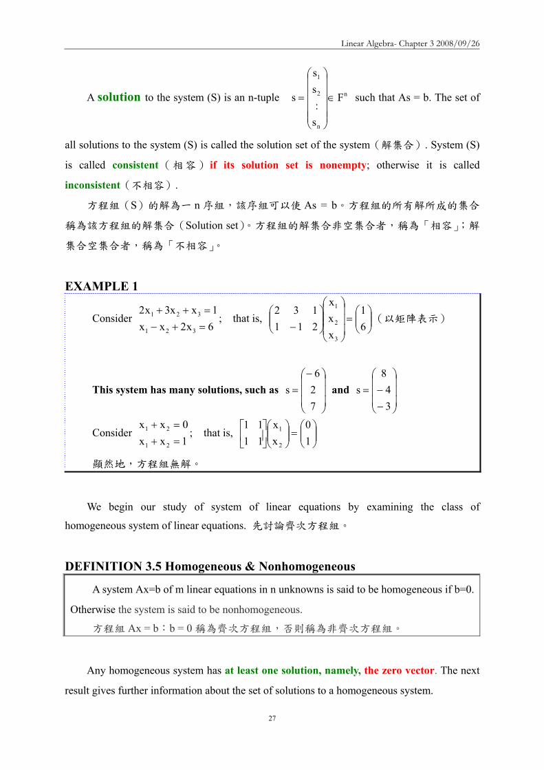
Linear Algebra- Chapter 3 20080926
31
因此 Ksube s +KH
反之假設 wisins +KH則 KH中存在一元素 k(kisinKH)使得 w = s + k
因 Aw = A(s + k) = As + Ak = b + 0 = b
故 wisinK 是 Ax = b 的解
因此s +KHsubeK
總結K=s +KH
EXAMPLE 3
Consider 4xxx7xx2x
321
321
minus=minusminus=++
The corresponding homogeneous system is the system in Example 2 It is easily
verified that ⎟⎟⎟
⎠
⎞
⎜⎜⎜
⎝
⎛=
411
s is a solution to the preceeding nonhomogeneous system So the
solution set of the system is ⎪⎭
⎪⎬
⎫
⎪⎩
⎪⎨
⎧isin
⎟⎟⎟
⎠
⎞
⎜⎜⎜
⎝
⎛minus+
⎟⎟⎟
⎠
⎞
⎜⎜⎜
⎝
⎛= Rt
32
1t
411
K by Theorem 39
⎟⎟⎟
⎠
⎞
⎜⎜⎜
⎝
⎛=
411
s 是非齊次方程組 Ax = b 的解
⎟⎟⎟
⎠
⎞
⎜⎜⎜
⎝
⎛minus32
1是齊次方程組的解
依據 Theorem 39 得知線性方程組 Ax = b 的解集合⎪⎭
⎪⎬
⎫
⎪⎩
⎪⎨
⎧isin
⎟⎟⎟
⎠
⎞
⎜⎜⎜
⎝
⎛minus+
⎟⎟⎟
⎠
⎞
⎜⎜⎜
⎝
⎛= Rt
32
1t
411
K
The following theorem will provide us with a means of computing solutions to certain
system of linear equations
Theorem 310~311 提供計算線性方程組的解的方法
Theorem 310 Let Ax = b be a system of n linear equations in n unknowns If A is invertible then the
Linear Algebra- Chapter 3 20080926
32
system has exactly one solution namely A-1b Conversely if the system has exactly one
solution then A is invertible
令 Ax = b 為含 n 個未知數n 個線性方程式的方程組若 A 為可逆則方程組
恰有一個解解為 A-1b反之若該方程組恰有一個解則 A 為可逆
【Proof】
Suppose that A is invertible
Substituting A-1b into system we have A(A-1b)=( AA-1)b = b
Thus A-1b is a solution
If s is an arbitrary solution then As = b
Multiplying both sides by A-1 gives s= A-1b
Thus the system has one and only one solution namely A-1b
假設 A 為可逆將 A-1b 代入方程組可得 A(A-1b)=( AA-1)b = b
故 A-1b 確為方程組的解
若 s 為方程組的任意解則 As = b
兩邊乘上 A-1可得 s= A-1b
因此方程組僅有唯一的解 A-1b
Conversely suppose that the system has exactly one solution s
Let KH denot the solution set for the corresponding homogeneous system Ax = 0
By Theorem 39 s = s + KH But it is so only if KH = 0 Thus N(LA) = 0 and
hence A is invertible
反之假設方程組恰有一個解 s
令 KH為相對應齊次方程組 Ax = 0 的解集合
依據 Theorem 39要能s = s + KH唯有 KH = 0
KH = 0即表示 N(LA) = 0故 A 為可逆
EXAMPLE 4 Consider the following system of three linear equations in three unknowns
1xx3x33x2x4x2
2x4x2
321
321
32
=++=++
=+
In Example 5 of Section 32 we compute the inverse of the coefficient matrix A of
this system Thus the system has exactly one solution namely
Linear Algebra- Chapter 3 20080926
33
⎟⎟⎟
⎠
⎞
⎜⎜⎜
⎝
⎛=
133242420
A⎟⎟⎟
⎠
⎞
⎜⎜⎜
⎝
⎛
+minus+minus+minus+minus+
=minus
41
83
83
21
43
41
43
85
81
1A
⎟⎟⎟
⎠
⎞
⎜⎜⎜
⎝
⎛
minus+minus
=⎟⎟⎟
⎠
⎞
⎜⎜⎜
⎝
⎛
⎟⎟⎟
⎠
⎞
⎜⎜⎜
⎝
⎛
+minus+minus+minus+minus+
==⎟⎟⎟
⎠
⎞
⎜⎜⎜
⎝
⎛minus
814587
41
83
83
21
43
41
43
85
81
1
3
2
1
132
bAxxx
Theorem 311 Let Ax = b be a system of linear equations Then the system is consistent (相容)if
and only if rank(A) = rank (A∣b) Matrix (A b) is called the augmented matrix o∣ f the
system Ax = b
令 Ax = b 為線性方程式方程組則此方程組至少有一個解的『若且唯若』條件
為 rank(A) = rank (A∣b) 矩陣(A∣b)稱為方程組 Ax = b 的增廣矩陣
【Proof】
To say that Ax = b has a solution is equivalent to saying that bisinR(LA)
In the proof of Theorem 35 we saw that R(LA ) = span(a1 a2 an) the span of the
column of A
Thus Ax = b has a solution if and only if bisinspan(a1 a2 an)
But bisinspan(a1 a2 an) if and only if span(a1 a2 an) = span(a1 a2 an b)
This last statement is equivalent to
dim (span(a1a2an)) = dim (span(a1a2an b))
So by Theorem 35 the preceeding equation reduces to rank(A) = rank (A∣b)
Ax = b 有一解相當於 bisinR(LA)即 b 屬於線性轉換 LA的 Range
在 Theorem 35 的證明中提到 R(LA ) = span(a1a2an)aj 為 A 的第 j 個行
(Column)即線性轉換 LA 的 Range 係由矩陣 A 的行(Column)所生成
因此 Ax = b 要有一個解的『若且唯若』條件為 bisinspan(a1 a2 an)
至於 bisinspan(a1 a2 an)之條件
bisinspan(a1a2an) 的『若且唯若』條件為 span(a1a2an) = span(a1a2an
b)
其條件相當於
Linear Algebra- Chapter 3 20080926
34
dim (span(a1a2an)) = dim (span(a1a2an b))
依據 Theorem 35該條件可簡化為 rank(A) = rank (A∣b)
Theorem 35 The rank of any matrix equals the maximum number of its linearly
independent columns that is the rank of a matrix is the dimension of the subspace
generated by its column任一矩陣的 Rank 等於其最大線性獨立行向量數目即矩陣的
Rank 是由矩陣的行向量生成的子空間的維度【LA Fn Fm】
EXAMPLE 5 Recall the system of equations
1xx0xx
21
21
=+=+
Since ⎟⎟⎠
⎞⎜⎜⎝
⎛=
1111
A and ⎟⎟⎠
⎞⎜⎜⎝
⎛=
111011
)bA(
rank(A) = 1 and rank (A b) = 2∣
Because the two ranks are unequal the system has no solutions
矩陣 A 與增廣矩陣(A∣b) 的 Rank 不同故方程組沒有解
EXAMPLE 6 We can use Theorem 311 to determine whether (3 3 2) is in the range of the linear
transformation T R3 R3 defined by T(a1 a2 a3) = (a1+a2+a3 a1-a2+a3 a1+a3)
利用 Theorem 311 來判斷 (3 3 2)是否在線性轉換 T 的 Range 中其中T R3
R3 定義為 T(a1 a2 a3) = (a1+a2+a3 a1-a2+a3 a1+a3)
Now (3 3 2)isinR(T) if and only if there exists a vector s = x1 x2 x3 in R3 such that
T(s)=(3 3 2) Such a vector s must be a solution to the system
2xx3xxx3xxx
31
321
321
=+=+minus=++
Since the ranks of the coefficient matrix and the augmented matrix of this system
are 2 and 3 respectively it follows that this system has no solutions Hence (3 3 2) notin
R(T)
(3 3 2)isinR(T) 的『若且唯若』的條件為存在一向量 s = x1 x2 x3isinR3 使得
T(s)=(3 3 2)
Linear Algebra- Chapter 3 20080926
35
向量 s 必須是 2xx3xxx3xxx
31
321
321
=+=+minus=++
的解
因係數矩陣⎟⎟⎟
⎠
⎞
⎜⎜⎜
⎝
⎛minus
101111111
的 Rank 為 2增廣矩陣⎟⎟⎟
⎠
⎞
⎜⎜⎜
⎝
⎛minus
233
101111111
的 Rank 為 3兩
者不相等故方程組無解(3 3 2) notin R(T)
Theorem 311 Let Ax = b be a system of linear equations Then the system is consistent
(相容)if and only if rank(A) = rank (A∣b) Matrix (A b) is called the ∣ augmented
matrix of the system Ax = b 令 Ax = b 為線性方程式方程組則此方程組至少有一個
解的『若且唯若』條件為 rank(A) = rank (A∣b) 矩陣(A∣b)稱為方程組 Ax = b 的
增廣矩陣
Application
In 1973 Wassily Leontief won the Nobel prize in economics for his work in developing
a mathematical model that can be used to describe various economic phenomena
1973 年Wassily Leontief 因研究一數學模式來描述各種經濟現象而獲頒諾貝爾經
濟獎
CLOSED MODEL
We begin by considering a simple society composed of three peoples (industries) ndash a
farmer who gows all the food a tailor who makes all the clothing and a carpenter who builds
all the housing We assume that each person sells to and buy from a central pool and that
everything produced is consumed Since no commodities either enter or leave the system this
case is referred to as the CLOSE MODEL
考慮一個單純社會的三種人生產食物的農夫製衣的裁縫師與蓋住屋的木匠
並假設採取集中聯營買賣且每一件產品皆付諸消費由於過程中沒有任何成品進入
或脫離這個系統所以稱為「封閉模式」
Each of these three individual consumes all three of the commodities produced in the
Linear Algebra- Chapter 3 20080926
36
society Suppose that the proportion of each of the commodities consumed by each person is
given in the following table
社會中每一位皆消費所生產的三種成品且每一種產品也都被三位所消費其消
費比例如下
食物 Food 衣物 Clothing 住屋 Housing
農夫 Farmer 040 020 020
裁縫師 Tailor 010 070 020
木匠 Carpenter 050 010 060
Let p1 p2 and p3 denote the incomes of the farmer tailor and carpenter respectively To
ensure that this society survives we require that the consumption of each individual equals
his or her income
令 p1p2 與 p3 分別表示農夫裁縫師與木匠的收入並為確保這個封閉社會可以
存活假設每一位的收入等於消費
Note that the farmer consumes 20 of the clothing Because the total cost of all clothing
is p2 the tailorrsquos income the amount spent by the farmer on clothing is 020 p2 Moreover the
amount spent by the farmer on food clothing and housing must equal the farmerrsquos income
and so we obtain the equation 040 p1 + 020 p2 + 030 p3 = p1
對農夫而言農夫的衣物消費佔 20然因所有衣物的消費總額 p2 等於裁縫師的
收入所以農夫在衣物上的消費為 020 p2且農夫在食物衣物與住屋的總消費要等
於農夫的收入 p1所以農夫的收入與消費關係式
040 p1 + 020 p2 + 020 p3 = p1
Similary equations describing the expenditures of the tailor and carpenter produce the
following system of linear equations
同理分別對裁縫師與木匠進行討論可獲得下列方程組
Linear Algebra- Chapter 3 20080926
37
040 p1 + 020 p2 + 020 p3 = p1
010 p1 + 070 p2 + 020 p3 = p2
050 p1 + 010 p2 + 060 p3 = p3
This system can be written as Ap = p
其中⎟⎟⎟
⎠
⎞
⎜⎜⎜
⎝
⎛=
3
2
1
ppp
p 且⎟⎟⎟
⎠
⎞
⎜⎜⎜
⎝
⎛=
600100500200700100200200400
A 稱為輸入-輸出(或消費)矩陣
(Input-output (or consumption) matrix)
Ap = p 稱為均衡條件(Equilibrium condition)
能否利用不等式 p ≦ p 來替代等式
At first it may seem reasonable to replace the equilibrium condition by the inequality
Ap ≦ p that is the requirement that consumption not exceed production But in fact Ap ≦ p implies that Ap = p in the closed model
For otherwise there exists a k for which
sumgt
jjkjk pAp
Hence since the columns of A sum to 1
sumsumsumsum ==gt
jj
i jjij
ii ppAp which is a contradiction (出現矛盾)
答案是在封閉系統中Ap ≦ p Ap = p
One solution to the homogeneous system (I ndash A) x = 0 which is equivalent to the
equilibrium condition is ⎟⎟⎟
⎠
⎞
⎜⎜⎜
⎝
⎛=
400350250
p
Linear Algebra- Chapter 3 20080926
38
齊次方程組(I ndash A) x = 0 或均衡條件的一個解為 ⎟⎟⎟
⎠
⎞
⎜⎜⎜
⎝
⎛=
400350250
p
We may interpret this to mean that the society survives if the farmer taior and carpenter
have incomes in the proportions 253540
⎟⎟⎟
⎠
⎞
⎜⎜⎜
⎝
⎛=
400350250
p 可以解釋為若農夫裁縫師與木匠收入比例為 253540則社會將
能生存下去
Theorem 312
Let A be an ntimesn input-output matrix having the form ⎟⎟⎠
⎞⎜⎜⎝
⎛=
EDCB
A where D is a 1times(n-
1) positive vector and C is an (n-1)times1 positive vector Then (I-A)x = 0 has a one-
dimensional solution set that is generated by a nonnegative vector
設 A 為 ntimesn 輸入-輸出矩陣 ⎟⎟⎠
⎞⎜⎜⎝
⎛=
EDCB
A 其中D 為 1times(n-1)正向量C 為
(n-1)times1 正向量則(I-A)x = 0 具有一維解集合且該解集合係由一非負向量所生成
Any input-output matrix with all positive entries satisfies the hypothesis of this theorem
任何輸入-輸出矩陣滿足 Theorem 312 的基本假設條件例如
⎟⎟⎟
⎠
⎞
⎜⎜⎜
⎝
⎛=
02502503502500650500750
A
OPEN MODEL
In the OPEN MODEL we assume that there is an outside demand for each of the
commodities produced Returning to our simple society let x1 x2 and x3 be the monetary
values of food clothing and housing produced with respective outside demands d1 d2 and d3
Let A be the 3times3 matrix such that Aij represents the amount of commodity i required to
Linear Algebra- Chapter 3 20080926
39
produce one monetary unit of commodity j Then the value of the surplus of food in the
society is x1 ndash (A11x1+A12x2+A13x3) that is the value of food produced minus the value of
food consumed while producing the three commodities The assumption that everything
produced is consumed gives us a similar equilibrium condition for the open model namely
that the surplus of each of the three commodities must equal the corresponding outside
demands Hence i
3
1jjiji dxAx =minussum
=
for j=1 2 3
在「開放模式」中我們假設每一產品皆有外來的需求在前述的單純社會裡
令 x1x2 與 x3 分別代表食物衣物與住屋的貨幣價值d1d2 與 d3 為食物衣物與住
屋的外來需求價值令 A 為 3times3 矩陣Aij 表示生產『一個貨幣單位』的產品 j 所需要
的產品 i 的價值於是此社會中食物的盈餘價值為 x1 ndash (A11x1+A12x2+A13x3)即食物的
價值減去生產食物衣物與住屋所需消耗的食物的價值意即生產出來的食物價值扣
掉用去生產食物衣物與住屋所消耗掉的價值)(A11A12A13 為生產一個貨幣單位
的食物 1衣物 2 與住屋 3 所需消耗的食物 1 數量A12x2 表示生產貨幣價值為 x2的衣物
所需要的食物價值)對每一種產品而言其盈餘價值等於外來的需求價值於是
i
3
1jjiji dxAx =minussum
=
for j=123
Suppose that 30 cents worth of food 10 cents worth of clothing and 30 cents worth of
housing are required for the production of $1 worth of food Similar suppose that 20 cents
worth of food 40 cents worth of clothing and 20 cents worth of housing are required for the
production of $1 worth of clothing Finally suppose that 30 cents worth of food 10 cents
worth of clothing and 30 cents worth of housing are required for the production of $1 worth
of housing Then the input-output matrix is
⎟⎟⎟
⎠
⎞
⎜⎜⎜
⎝
⎛=
300200300100400100300200300
A
假設生產價值 1 元的食物需要價值 30 分的食物(A11 = 03)價值 10 分的衣物
(A21 = 01)及價值 30 分的住屋(A31 = 03)生產價值 1 元的衣物需要價值 20 分的
食物(A12 = 02)價值 40 分的衣物(A22 = 04)及價值 20 分的住屋(A32 = 02)生
Linear Algebra- Chapter 3 20080926
40
產價值 1 元的住屋需要價值 30 分的食物(A13 = 03)價值 10 分的衣物(A23 = 01)
及價值 30 分的住屋(A33 = 03)於是輸入輸出矩陣 A 為
⎟⎟⎟
⎠
⎞
⎜⎜⎜
⎝
⎛=
300200300100400100300200300
A
若食物的外來需求值為 300 億元衣物為 200 億元住屋值為 1 百億元則
⎟⎟⎟
⎠
⎞
⎜⎜⎜
⎝
⎛=
⎟⎟⎟
⎠
⎞
⎜⎜⎜
⎝
⎛
⎟⎟⎟
⎠
⎞
⎜⎜⎜
⎝
⎛
minusminusminusminusminusminus
=minus=
minus
minus
700600900
100200300
700200300100600100300200300
d)AI(x
1
1
⎟⎟⎟
⎠
⎞
⎜⎜⎜
⎝
⎛=
700600900
x 表示要滿足外來需求必須生產的食物價值為 900 億元衣物價值為
600 億元住屋價值為 700 億元
Theorem
Let AX = Y be a system of n linear equations in n variables If Andash1 exists the
solution is unique and is given by X = Andash1Y
【Proof】
Substitute X = Andash1Y into the matrix equation
AX = A(Andash1Y) = (AAndash1)Y = InY = Y
The solution is unique
Let X1 be any solution thus AX1 = Y Multiplying both sides of this equation by Andash1
gives
Andash1AX1= Andash1Y InX1 = Andash1Y X1 = Andash1Y
Linear Algebra- Chapter 3 20080926
41
Example Example 1212
2x5x3x3x5x3x21x2x x
321
321
321
minus=++minus=minusminus=minusminus
⎥⎥⎥
⎦
⎤
⎢⎢⎢
⎣
⎡
minus=
⎥⎥⎥
⎦
⎤
⎢⎢⎢
⎣
⎡
⎥⎥⎥
⎦
⎤
⎢⎢⎢
⎣
⎡
minusminusminusminusminus
231
xxx
531532211
3
2
1
Solve the system of equations
This system can be written in the following matrix form
⎥⎥⎥
⎦
⎤
⎢⎢⎢
⎣
⎡
minus⎥⎥⎥
⎦
⎤
⎢⎢⎢
⎣
⎡
minusminusminusminusminus
=
⎥⎥⎥
⎦
⎤
⎢⎢⎢
⎣
⎡minus
231
531532211
xxx 1
3
2
1
If the matrix of coefficients is invertible the unique solutionIf the matrix of coefficients is invertible the unique solution isis
Example Example 2222
1 2 1 issolution unique The 321 =minus== xxx
⎥⎥⎥
⎦
⎤
⎢⎢⎢
⎣
⎡minus=
⎥⎥⎥
⎦
⎤
⎢⎢⎢
⎣
⎡
minus⎥⎥⎥
⎦
⎤
⎢⎢⎢
⎣
⎡
minusminusminus=
⎥⎥⎥
⎦
⎤
⎢⎢⎢
⎣
⎡
121
231
123135110
xxx
3
2
1
⎥⎥⎥
⎦
⎤
⎢⎢⎢
⎣
⎡
minusminusminus=
⎥⎥⎥
⎦
⎤
⎢⎢⎢
⎣
⎡
minusminusminusminusminus
=
minus
minus
123135110
531532211
A
1
1
The The LeontiefLeontief IO Model in IO Model in Economics Economics 1515
The Leontief input-output model is used to analyze the interdependence of economics Wassily Leontief received a Nobel Prize in 1973 for his work in thie fieldThe practical applications of this model have proliferated until it has now become a standard tool for investigating economic structures ranging from cities and corporation to states and countriesConsider an economics situation that involves ninterdependent industries The output of any one industry is needed as input by other industries and even possibly by the industry itself
The The LeontiefLeontief IO Model in IO Model in Economics Economics 2525
How a mathematical model involving a system of linear equations can be constructed to analyze such a situationAssume that each industry produces one commodity Let aij denote the amount of input of a certain commodity i to produce unit output of commodity j In our model let the amounts of input and output be measured in dollars Thus for example a34 = 045 means that 45 centsrsquo worth of commodity 3 is required to produce one dollarrsquos worth of commodity 4
The The LeontiefLeontief IO Model in IO Model in Economics Economics 3535
aij = amount of commodity i in one dollar of commodity jaij =生產一元價值的j產品需要耗用的i產品價值
The elements aij called input coefficients define a matrix A called the input-output matrix which describes the interdependence of the industriesExtending the model to include an open sector (all non-producing sectors) The product of industries may go not only into other producing industries but also into other non-producing sectors of the economy such as consumers and governments
The The LeontiefLeontief IO Model in IO Model in Economics Economics 4545
di = demand of the open sectors from industry ixi=total output of industry I necessary to meet demands of all n industries and the open sector
sectoropen of demand
nindustry of demand
2industry of demand
22
1industry of demand
11
industry ofoutput total
ininii
i
i dxaxaxax ++sdotsdotsdot++=
output ofportion sectoropen
output ofportion tryinterindusoutput total
DAXX +=Demand matrixDemand matrix
Output matrixOutput matrix
The The LeontiefLeontief IO Model in IO Model in Economics Economics 5555
Applying the model to the economy of a country X Applying the model to the economy of a country X represents the total output of each of the producing sectors represents the total output of each of the producing sectors of the economy and AX describes the contributions made of the economy and AX describes the contributions made by the various sectors to fulfilling the intersectional input by the various sectors to fulfilling the intersectional input requirements of the economyrequirements of the economyD is equal to (XD is equal to (X--AX) the difference between total output AX) the difference between total output X and industry transaction AXX and industry transaction AXD is thus the gross national product of the economyD is thus the gross national product of the economy
Example Example 1414
Consider an economy consisting of three industries having Consider an economy consisting of three industries having the following inputthe following input--output matrix output matrix AA Determine the output Determine the output levels required of the industries to meet the demands of levels required of the industries to meet the demands of the other industries and of the open sector in each casethe other industries and of the open sector in each case
in turn 321812
and 896
1612
9
5100
021
21
103
51
51
⎥⎥⎦
⎤
⎢⎢⎣
⎡
⎥⎥⎦
⎤
⎢⎢⎣
⎡
⎥⎥⎦
⎤
⎢⎢⎣
⎡=
⎥⎥⎥
⎦
⎤
⎢⎢⎢
⎣
⎡
= DA
The unit of The unit of DD are millions of dollarsare millions of dollars
Linear Algebra- Chapter 3 20080926
42
Example Example 2424
We wish to compute the output levels X that correspond to We wish to compute the output levels X that correspond to the various open sector demands D X is given by the the various open sector demands D X is given by the equation X = AX + D Rewritten as followsequation X = AX + D Rewritten as follows
X ndash AX = D rArr (I ndash A)X = D rArr X = (I ndash A) ndash1 D
⎥⎥⎥
⎦
⎤
⎢⎢⎢
⎣
⎡
=⎥⎥⎥
⎦
⎤
⎢⎢⎢
⎣
⎡
minus⎥⎥⎦
⎤
⎢⎢⎣
⎡=minus minus
minusminus
5400
021
21
103
51
54
5100
021
21
103
51
31
100010001
get We AI
⎥⎥⎥
⎦
⎤
⎢⎢⎢
⎣
⎡
=minus minus
4500
038
35
85
32
35
1)( AI
output ofingcorrespond valuesvarious
4500
038
35
85
32
35
)(
401020883957522133
32816189121269
)(
1
1
DAI
DAIX
minus
minus
minusuarruarruarruarruarruarruarr
⎥⎥⎦
⎤
⎢⎢⎣
⎡=
⎥⎥⎦
⎤
⎢⎢⎣
⎡
⎥⎥⎥
⎦
⎤
⎢⎢⎢
⎣
⎡
=minus=
Example Example 3434
By using Gauss-Jordan elimination
dollars of milliond are units The
40
15674
and 106629
209946
are 321812
and 896
1612
9
⎥⎥⎥
⎦
⎤
⎢⎢⎢
⎣
⎡
⎥⎥⎥
⎦
⎤
⎢⎢⎢
⎣
⎡
⎥⎥⎥
⎦
⎤
⎢⎢⎢
⎣
⎡
⎥⎥⎥
⎦
⎤
⎢⎢⎢
⎣
⎡
⎥⎥⎥
⎦
⎤
⎢⎢⎢
⎣
⎡
⎥⎥⎥
⎦
⎤
⎢⎢⎢
⎣
⎡
Example Example 4444
The output levels necessary to meet the demandsThe output levels necessary to meet the demands
IAAAIAI m =++++minus ))(( 2 L
mAAAIAI ++++=minus minus L21)(
Computing (IComputing (I--A) A) --11
1m
m2m2
m2
AI)AAAI(A)AAAI(I
)AAAI)(AI(
+minus=++++minus++++=
++++minusLL
L
NOTE 0A 1m rarr+
Population Movement Population Movement 1313
In 2000 58 million of people live in cities and 142 million of In 2000 58 million of people live in cities and 142 million of people people live in the surrounding suburbs Represent this information by tlive in the surrounding suburbs Represent this information by the he matrix matrix
The probability of a person staying in the city was 096 Thus tThe probability of a person staying in the city was 096 Thus the he probability of moving to the suburbs was 004 probability of moving to the suburbs was 004 The probability of a person moving to the city was 001 the The probability of a person moving to the city was 001 the probability of remaining in suburbia was 099probability of remaining in suburbia was 099
suburbcity
990040010960
suburbcity (to))from(
⎥⎦
⎤⎢⎣
⎡=P
⎥⎦
⎤⎢⎣
⎡=
14258
X0
City population in 2001 = people who remained from 2000 + peopleCity population in 2001 = people who remained from 2000 + peoplewho moved in from the suburbs = ( 096 who moved in from the suburbs = ( 096 timestimes 58 ) + (001 58 ) + (001 timestimes 142 ) = 142 ) = 571 million571 millionSuburban population in 2001 = people who moved in from the city Suburban population in 2001 = people who moved in from the city + people who stayed from 2000 = ( 004 + people who stayed from 2000 = ( 004 timestimes 58 ) + (099 58 ) + (099 timestimes 142 ) = 142 ) = 1429 million1429 millionCan arrive at these numbers using matrix multiplicationCan arrive at these numbers using matrix multiplication
⎥⎦
⎤⎢⎣
⎡=⎥
⎦
⎤⎢⎣
⎡⎥⎦
⎤⎢⎣
⎡==
9142157
14258
990040010960
PXX 01
Population Movement Population Movement 2323
Population Movement Population Movement 3333
Assume that the population flow represented by the matrix P is unchanged over the years The population distribution X2 after 2 years is given by X2 = P X1 = P2 X0 In general
Pn is called the n-step transition matrix The (ij)th element of Pngives the probability of going from state j to state i in n stepsFor example
in
ni XPX =+
suburbcity
960150040850
P
suburbcity (to))from(
4
⎥⎦
⎤⎢⎣
⎡=
The probability of living in the city in The probability of living in the city in 2000 and being in the suburbs 4 years 2000 and being in the suburbs 4 years later is 015later is 015
Markov ChainsMarkov Chains
The probabilities in the above model depend only on the The probabilities in the above model depend only on the current state of a person whether the person is living in the current state of a person whether the person is living in the city or in suburbiacity or in suburbiaThis type of model in which the probability of going from This type of model in which the probability of going from one state to another depends only on the current state one state to another depends only on the current state rather than on a more complete historical description is rather than on a more complete historical description is called a called a Markov chainMarkov chainMarkov chains are useful tools for scientists in many Markov chains are useful tools for scientists in many fields such as geneticsfields such as genetics
Linear Algebra- Chapter 3 20080926
43
GeneticsGenetics 1414
Genetics is the branch of biology that deals with Genetics is the branch of biology that deals with heredity heredity (遺傳)(遺傳) It is the study of units called It is the study of units called genes which determine the characteristics living genes which determine the characteristics living things inherit from their parents The inheritance things inherit from their parents The inheritance (遺傳)(遺傳)of such traitsof such traits(特徵)(特徵)as sex height eye as sex height eye color and hair color of human beings and such color and hair color of human beings and such traits as petaltraits as petal(花瓣)(花瓣) color and leaf shape of color and leaf shape of plants are governed by genesplants are governed by genesIn medicine agricultureIn medicine agriculturehelliphellip
GeneticsGenetics 2424
The traits of guinea pigsThe traits of guinea pigs(天竺鼠)(天竺鼠)are long hair and short hairare long hair and short hairThe length of hair is governed by a pair of gene which we denoteThe length of hair is governed by a pair of gene which we denote A A and aand aA guinea pig may have any one of the combination of AA A guinea pig may have any one of the combination of AA AaAa or or aaaa Each of these classes is called a genotypeEach of these classes is called a genotype(基因型)(基因型)The AA type guinea pig is indistinguishable in appearance from tThe AA type guinea pig is indistinguishable in appearance from the he AaAa type type ndashndash both have long hair both have long hair ndashndash whereas the whereas the aaaa type has short hairtype has short hairThe A gene is said to dominate the a geneThe A gene is said to dominate the a geneAn animal is called dominant An animal is called dominant (顯性)(顯性)if it has AA genes hybridif it has AA genes hybrid(混種)(混種) with with AaAa genes and recessive genes and recessive (隱性)(隱性)with with aaaa genesgenes
GeneticsGenetics 3434
When two guinea pigs are crossed the offspring inherits one genWhen two guinea pigs are crossed the offspring inherits one gene e from each parent in random mannerfrom each parent in random mannerGiven the genotype of the parents we can determine the Given the genotype of the parents we can determine the probabilities of the genotype of the offspringprobabilities of the genotype of the offspring
AA+AA AA+AA probabilities of AA probabilities of AA AaAa and and aaaa are 10and 0are 10and 0Aa+AAAa+AA probabilities of AA probabilities of AA AaAa and and aaaa are are frac12frac12 frac12frac12 and 0 and 0aa+AAaa+AA probabilities of AA probabilities of AA AaAa and and aaaa are 0 1 and 0are 0 1 and 0
This series of experiments is a Markov chain having transition This series of experiments is a Markov chain having transition matrixmatrix
aaAaAA
00012100211
P
aaAaAA
⎥⎥⎥
⎦
⎤
⎢⎢⎢
⎣
⎡=
GeneticsGenetics 4444
Assume an initial population of guinea pigs made up of an Assume an initial population of guinea pigs made up of an equal number of each genotypeequal number of each genotype
⎥⎥⎥
⎦
⎤
⎢⎢⎢
⎣
⎡=
313131
X0
The fractions of following generations are
⎥⎥⎥
⎦
⎤
⎢⎢⎢
⎣
⎡=
⎥⎥⎥
⎦
⎤
⎢⎢⎢
⎣
⎡=
⎥⎥⎥
⎦
⎤
⎢⎢⎢
⎣
⎡=
⎥⎥⎥
⎦
⎤
⎢⎢⎢
⎣
⎡=
01611615
X08187
X04143
X02121
X 4321
AAAAAaAaaaaa
3-4 Systems of Linear Equations ndash Computational Aspects
DEFINITION 36 Equivalent
Two systems of linear equations are called equivalent if they have the same solution
set
兩個線性方程組稱為等價意指兩者具有相同的解集合
Elementary Transformations Transformation called elementary transformations can be used to change a system of
linear equations into another system of linear equations that have the same solution
These transformations are used to solve system of linear equations by eliminating
variables
The equivalent transformations used in terms of matrix are called ELEMENTARY
ROW OPERATION
Linear Algebra- Chapter 3 20080926
44
Equivalent System Systems of equations that are related through elementary transformations are called
equivalent systems
Matrices that are related through elementary row operations are called row equivalent
matrices
The symbol asymp is used to indicate equivalence in both cases
Theorem 313 Let Ax = b be a system of m linear equations in n unknowns and let C be an invertible
mtimesm matrix Then the system (CA)x = Cb is equivalent to Ax = b
設 Ax = b 為含 n 個未知數m 個線性方程式的方程組若 C 為可逆的mtimesm
矩陣則(CA)x = Cb 等價於 Ax = b
【Proof】
Let K be the solution set for Ax = b and Krsquo the solution set for (CA)x = Cb If wisinK
then Aw = b So (CA)w = Cb and hence wisinKrsquo Thus KsubeKrsquo
Conversely if wisinKrsquo then (CA)w = Cb Hence Aw = C-1(CA)w = C-1(Cb) = b so
wisinK Thus KrsquosubeK and therefore K=Krsquo
設 K 為 Ax = b 的解集合且 Krsquo為(CA)x = Cb 的解集合
若 wisinK則 Aw = b (CA)w = Cb故 wisinKrsquo於是 KsubeKrsquo
反之若 wisinKrsquo則(CA)w = Cb Aw = C-1(CA)w = C-1(Cb) = b故 wisinK於是
KrsquosubeK因此K=Krsquo
Corollary Let Ax = b be a system of m linear equations in n unknowns If (Arsquo brsquo) is obtained ∣
from from (A b) by a finite number of elementary row operations then the system Arsquox = ∣
brsquo is equivalent to the original system
設 Ax = b 為含 n 個未知數m 個線性方程式的方程組若(Arsquo brsquo) ∣ 是由(A b) ∣
經過有限次數的基本列運算而得則 Arsquox = brsquo 等價於 Ax = b即兩者具有相同的解
集合
【Proof】
Suppose that (Arsquo brsquo) is obtained from (A b) by elementary row operations These ∣ ∣
Linear Algebra- Chapter 3 20080926
45
may be executed by multiplying (A b) by elementary mtimesm matrices E∣ 1 E2hellipEp Let
C=EphellipE2E1 then (Arsquo brsquo) = C(A b) = (CA Cb)∣ ∣ ∣
Since each Ei is invertible so is C Now Arsquo = CA and brsquo = Cb Thus by Theorem 313
the system Arsquox = brsquo is equivalent to the system Ax = b
設(Arsquo brsquo)∣ 是由(A b)∣ 經過基本列運算取得即以基本 mtimesm 矩陣 E1 E2hellipEp
乘上 (A b)∣ (Arsquo brsquo) = C(A b) = (CA Cb∣ ∣ ∣ )其中C=EphellipE2E1
因 Ei 可逆故 C 亦為可逆 Arsquo = CA 且 brsquo = Cb
依據 Theorem 313Arsquox = brsquo 等價於 Ax = b
Theorem 313 Let Ax = b be a system of m linear equations in n unknowns and let C be an
invertible mtimesm matrix Then the system (CA)x = Cb is equivalent to Ax = b 設 Ax = b
為含 n 個未知數m 個線性方程式的方程組若 C 為可逆的mtimesm 矩陣則(CA)x
= Cb 等價於 Ax = b
We now describe a method for solving any stystem of linear equations Consider for
example the system of linear equations
探討解線性方程組的方法hellip
2xxx2x3xxx1x2x3x2x3
4321
321
4321
=minus++=++=minus++
First we form the augmented matrix ⎟⎟⎟
⎠
⎞
⎜⎜⎜
⎝
⎛
minus
minus
231
112101112323
(增廣矩陣)
Interchanging the first and third rows ⎟⎟⎟
⎠
⎞
⎜⎜⎜
⎝
⎛
minus
minus
132
132301111121
(第 13 列互調)
Adding -1 times the first row to the second row and then add -3 times the first row to
the third row ⎟⎟⎟
⎠
⎞
⎜⎜⎜
⎝
⎛
minusminusminus
minus
512
104010101121
(第 1 列乘上 -1 加到第 2 列再以 -3 乘上
第 1 列加到第 3 列)
Linear Algebra- Chapter 3 20080926
46
Multiplying the second row by -1 ⎟⎟⎟
⎠
⎞
⎜⎜⎜
⎝
⎛
minusminus
minusminusminus
51
2
104010101121
(第 2 列乘上 -1)
Adding four times the second row to the third row ⎟⎟⎟
⎠
⎞
⎜⎜⎜
⎝
⎛
minusminus
minusminusminus
91
2
300010101121
(4 乘上第 2
列加到第 3 列)
Multiplying the third row by -13 ⎟⎟⎟
⎠
⎞
⎜⎜⎜
⎝
⎛minusminus
minus
31
2
100010101121
(第 3 列乘上 -13)
Adding the third row to the first and second rows to obtain zeros in row 1 column 4
and row 2 column 4 ⎟⎟⎟
⎠
⎞
⎜⎜⎜
⎝
⎛
325
100000100121
(將第 3 列加到第 1 列及第 2 列)
Adding -2 times the second row to the first row in order to make the first row second
column entry become zero ⎟⎟⎟
⎠
⎞
⎜⎜⎜
⎝
⎛
321
100000100101
(將第 2 列乘以 -2 再加至第 1 列)
We have now obtained the desired reduction of the augmented matrix
⎟⎟⎟
⎠
⎞
⎜⎜⎜
⎝
⎛
321
100000100101
是化簡後的增廣矩陣
This matrix corresponds to the system of linear equations
對應的線性方程組為
2x3x1xx
4
2
31
===+
By Corollary to Theorem 313 this system is equivalent to the original system But this
system is easily solved Obviously x2 = 2 and x4 = 3 Moreover x1 and x3 can be any values
Linear Algebra- Chapter 3 20080926
47
provided their sum is 1 Letting x3 = t we then have x1 = 1 ndash t Thus an arbitray solution to the
original system has the form
依據 Corollary to Theorem 313 化簡後的方程組與原方程組等值此方程組的解為
x2 = 3x4 = 3x1 + x3 = 1於是原方程組的任意解可以寫成
⎟⎟⎟⎟⎟
⎠
⎞
⎜⎜⎜⎜⎜
⎝
⎛minus
+
⎟⎟⎟⎟⎟
⎠
⎞
⎜⎜⎜⎜⎜
⎝
⎛
=
⎟⎟⎟⎟⎟
⎠
⎞
⎜⎜⎜⎜⎜
⎝
⎛ minus
0101
t
3021
3t2
t1
Observe that
⎪⎪⎭
⎪⎪⎬
⎫
⎪⎪⎩
⎪⎪⎨
⎧
⎟⎟⎟⎟⎟
⎠
⎞
⎜⎜⎜⎜⎜
⎝
⎛minus
0101
is a basis for the homogeneous system of equations
corresponding to the given system
其中
⎪⎪⎭
⎪⎪⎬
⎫
⎪⎪⎩
⎪⎪⎨
⎧
⎟⎟⎟⎟⎟
⎠
⎞
⎜⎜⎜⎜⎜
⎝
⎛minus
0101
是齊次方程組解集合的一組基底
Gauss-Jordan Elimination
Let A be an n times n matrix
1 Adjoin the identity n times n matrix In to A to form the matrix [A In]
2 Compute the reduced echelon form of [A In]
(1) If the reduced echelon form is of the type [In B] then B is the inverse of A
(2) If the reduced echelon form is not of the type [In B] in that the first n times n
submatrix is not In then A has no inverse
An n times n matrix A is invertible if and only if its reduced echelon form is In
DEFINITION 37 Reduced Row Echelon Form
A matrix is said to be in reduced row echelon form if the following three conditions
are satisfied
Linear Algebra- Chapter 3 20080926
48
一個矩陣可以被稱為簡約列梯形式必須具備有下列三條件
(a) Any row containing a nonzero entry preceeds any row in which all the entries are
zero (if any)
含有非零元素的任一列排在全含零元素的任一列前面(儘可能)
(b) The first nonzero entry in each row in the only nonzero entry in its column
各列中第一個非零元素為其所在行中唯一的非零元素
(c) The first nonzero entry in each row is 1 and it occurs in a column to thr right of the
first nonzero entry in the preceeding row
各列中第一個非零元素為 1 且它出現在前一列中第一個非零元素的右邊某一
行中
Reduced Echelon Form A matrix is in reduced echelon form if
1 Any rows consisting entirely of zeros are grouped at the bottom of the matrix
2 The first nonzero element of each other row is 1 This element is called a leading 1
3 The leading 1 of each row after the first is positioned to the right of the leading 1 of
the previous row
4 All other elements in a column that contains a leading 1 are zero
Theorem 314 Gaussian Elimination Transformation Gaussian elimination transform any matrix into its reduced row echelon form
利用 Gaussian elimination 將矩陣轉換成簡約列梯形式
We now describe a method for solving a system in which the augmented matrix is in
reduced row echelon form To illustrate this procedure we consider the system
14x8x3x2x2x28x5x2xxx6x3xxxx17x9x4xx3x2
54321
54321
54321
54321
=minus+++=minus+++=minus+++=minus+++
Linear Algebra- Chapter 3 20080926
49
for which the augmented matrix is
⎟⎟⎟⎟⎟
⎠
⎞
⎜⎜⎜⎜⎜
⎝
⎛
minusminusminusminus
1486
17
83222521113111194132
(增廣矩陣)
Applying Gaussian elimination to the augmented matrix of the system produces the
following sequence of matrices
利用 Gaussian elimination method 處理增廣矩陣
⎟⎟⎟⎟⎟
⎠
⎞
⎜⎜⎜⎜⎜
⎝
⎛
minusminusminusminus
1486
17
83222521113111194132
⎟⎟⎟⎟⎟
⎠
⎞
⎜⎜⎜⎜⎜
⎝
⎛
minusminusminusminus
148
176
83222521119413231111
⎟⎟⎟⎟⎟
⎠
⎞
⎜⎜⎜⎜⎜
⎝
⎛
minusminus
minus
0213
0000021000
1011020201
The system of linear equations corresponding to thus last matrix is
對應最後矩陣的線性方程組 2x2x
1xxx3x2x2x
54
532
531
=minus=+minus=minus+
Assign x3 = t1 x5 = t2
2t22x2x1tt1xxx
3t2t23x2x2x
254
21532
21531
+=+=+minus=+minus=
++minus=++minus=
Thus an arbitray solution s is of the form
於是任意解 s 具有下列形式
s =
⎟⎟⎟⎟⎟⎟
⎠
⎞
⎜⎜⎜⎜⎜⎜
⎝
⎛minus
+
⎟⎟⎟⎟⎟⎟
⎠
⎞
⎜⎜⎜⎜⎜⎜
⎝
⎛minus
+
⎟⎟⎟⎟⎟⎟
⎠
⎞
⎜⎜⎜⎜⎜⎜
⎝
⎛
=
⎟⎟⎟⎟⎟⎟
⎠
⎞
⎜⎜⎜⎜⎜⎜
⎝
⎛
+
+minus++minus
=
⎟⎟⎟⎟⎟⎟
⎠
⎞
⎜⎜⎜⎜⎜⎜
⎝
⎛
1201
2
t
00112
t
02013
t2t2
t1tt
3t2t2
xxxxx
21
2
2
1
21
21
5
4
3
2
1
where t1t2isinR
Linear Algebra- Chapter 3 20080926
50
Notice that
⎪⎪⎪
⎭
⎪⎪⎪
⎬
⎫
⎪⎪⎪
⎩
⎪⎪⎪
⎨
⎧
⎟⎟⎟⎟⎟⎟
⎠
⎞
⎜⎜⎜⎜⎜⎜
⎝
⎛minus
⎟⎟⎟⎟⎟⎟
⎠
⎞
⎜⎜⎜⎜⎜⎜
⎝
⎛minus
1201
2
00112
is a basis for the solution set of the corresponding
homogeneous system of equation and
⎟⎟⎟⎟⎟⎟
⎠
⎞
⎜⎜⎜⎜⎜⎜
⎝
⎛
02013
is a particular solution to the original system
⎪⎪⎪
⎭
⎪⎪⎪
⎬
⎫
⎪⎪⎪
⎩
⎪⎪⎪
⎨
⎧
⎟⎟⎟⎟⎟⎟
⎠
⎞
⎜⎜⎜⎜⎜⎜
⎝
⎛minus
⎟⎟⎟⎟⎟⎟
⎠
⎞
⎜⎜⎜⎜⎜⎜
⎝
⎛minus
1201
2
00112
是齊次方程組解集合的一組基底
⎟⎟⎟⎟⎟⎟
⎠
⎞
⎜⎜⎜⎜⎜⎜
⎝
⎛
02013
是原方程組的特別解
EXAMPLE 1
The matrix ⎟⎟⎟
⎠
⎞
⎜⎜⎜
⎝
⎛
101010011
is not in reduced row echelon form
因為第一行含有第一個非零元素在第一列但第一行尚含有其他非零元素
The matrix ⎟⎟⎟
⎠
⎞
⎜⎜⎜
⎝
⎛
110010012010
is not in reduced row echelon form
因為第一列第一個非零元素不在第一列第一個非零元素的右邊
The matrix ⎟⎟⎠
⎞⎜⎜⎝
⎛010002
is not in reduced row echelon form
因為第一列的第一個非零元素不是 1
Linear Algebra- Chapter 3 20080926
51
Reduced Echelon FormReduced Echelon Form
⎥⎥⎥
⎦
⎤
⎢⎢⎢
⎣
⎡
910030107001
⎥⎥⎥
⎦
⎤
⎢⎢⎢
⎣
⎡
100001000041
⎥⎥⎥
⎦
⎤
⎢⎢⎢
⎣
⎡
000210801
Not in Reduced Echelon Form
⎥⎥⎥
⎦
⎤
⎢⎢⎢
⎣
⎡
310000004021
⎥⎥⎥
⎦
⎤
⎢⎢⎢
⎣
⎡
100000430003021
⎥⎥⎥⎥
⎦
⎤
⎢⎢⎢⎢
⎣
⎡
0000210030108071
In Reduced Echelon Form
Use GaussUse Gauss--Jordan elimination to Jordan elimination to find reduced echelon formfind reduced echelon form 1313
Step 1 Interchange rows if necessary to bring a nonzero Step 1 Interchange rows if necessary to bring a nonzero element to the top of the first nonzero column This nonzero element to the top of the first nonzero column This nonzero element is called a pivotelement is called a pivot
⎥⎥⎦
⎤
⎢⎢⎣
⎡
minusminus
minus
1211244129333
22200
⎥⎥⎥
⎦
⎤
⎢⎢⎢
⎣
⎡
minusminus
minus
harrasymp
121124422200
129333
R2R1
Use GaussUse Gauss--Jordan elimination to Jordan elimination to find reduced echelon formfind reduced echelon form 2323
Step 2 Create a 1 in the pivot location by multiplying the Step 2 Create a 1 in the pivot location by multiplying the pivot row by 1pivotpivot row by 1pivot
Step 3 Create zero elsewhere in the pivot column by adding Step 3 Create zero elsewhere in the pivot column by adding suitable multiples of the pivot row to all other rows of the suitable multiples of the pivot row to all other rows of the matrixmatrix
⎥⎥⎥
⎦
⎤
⎢⎢⎢
⎣
⎡
minusminusminus
minus
minus+asymp
412002220043111
4)R1(R3
⎥⎥⎦
⎤
⎢⎢⎣
⎡
minusminus
minus
⎟⎠⎞
⎜⎝⎛asymp
12112442220043111
R13
1
The matrix is the reduced echelon form of the given matrixThe matrix is the reduced echelon form of the given matrix
Use GaussUse Gauss--Jordan elimination to Jordan elimination to find reduced echelon formfind reduced echelon form 3333
Step 4 Cover the pivot row and all rows above it Repeat Steps Step 4 Cover the pivot row and all rows above it Repeat Steps 1 1 and 2 for the remaining and 2 for the remaining submatrixsubmatrix Repeat Step 3 for the whole Repeat Step 3 for the whole matrix Continue until the reduced echelon form is reachedmatrix Continue until the reduced echelon form is reached
⎥⎥⎥
⎦
⎤
⎢⎢⎢
⎣
⎡
minusminus
+minus+asymp
⎥⎥⎥
⎦
⎤
⎢⎢⎢
⎣
⎡
minusminus
minus++asymp
⎥⎥⎥
⎦
⎤
⎢⎢⎢
⎣
⎡
minusminusminus
minus
⎟⎠⎞
⎜⎝⎛
asymp
⎥⎥⎥
⎦
⎤
⎢⎢⎢
⎣
⎡
minusminusminus
minus
6100050100
170011
R3R22)R3(R1
610001110052011
R2)2(R3R2R1
412001110043111
R221
412002220043111
Theorem 315 Let Ax = b be a system of r nonzero equations is in n unknown Suppose that rank(A)
= rank (A b)∣ and that (A b)∣ is in reduced row echelon form Then
設 Ax = b 為含有 n 個未知數r 個非零方程式的方程組假設 rank(A) = rank
(A b)∣ 且 (A b)∣ 為簡約列梯形式於是
(a) rank(A) = r
(b) If the general solution obtained by the procedure above is of the form s = s0 + t1u1
+ t2u2 +hellip+ tn-run-r then u1 u2hellip un-r is a basis for the solution set of the
corresponding homogeneous system and s0 is a solution to the original system 由
前述方法所得的 General solution 具有下列形式
s = s0 + t1u1 + t2u2 +hellip+ tn-run-r
其中u1 u2hellip un-r為齊次方程組 Ax = 0 的解集合的一組基底且 s0 為原方
程組的一個解)
【Proof】
Since (A b)∣ is in reduced row echelon form (A b)∣ must have r nonzero rows
Clearly these rows are linearly independent by the definition of the reduced row echelon
Linear Algebra- Chapter 3 20080926
52
form and so rank (A b)∣ = r Thus rank(A) = r
Let K be the solution set for Ax = b and let KH be the solution set for Ax = 0 Setting
t1 = t2 =hellip= tn-r = 0 we see that s = s0isinK But by Theorem 39 K = s +KH Hence
KH = - s0+K = span(u1 u2hellip un-r )
Because rank(A) = r we have dim(KH) = n-r Thus since dim(KH) = n-r and KH is
generated by a set u1 u2hellip un-r containing at most n-r vectors that is a basis for KH
由於(A b)∣ 具有簡約列梯形式因此(A b)∣ 必定具有 r 個非零列由簡約列梯形
式的定義得知 r 個非零列為線性獨立故 rank (A b)∣ = rrank(A) = r
令 K 為 Ax = b 的解集合 KH 為 Ax = 0 的解集合
假設 t1 = t2 =hellip= tn-r = 0(u1 u2hellip un-r非 KH的基底)則 s = s0isinK
依據 Theorem 39K = s +KH KH = - s0+K = span(u1 u2hellip un-r )
因 rank(A) = r所以 dim(KH) = n - r 且 KH 是由u1 u2hellip un-r 所生成
故原假設「t1 = t2 =hellip= tn-r = 0」不成立
因此 KH含有最多 n - r 個向量且這些向量為 KH的基底
Theorem 39 Let K be the solution set of a system of linear equations Ax = b and let KH be
the solution set of the corresponding homogeneous system Ax = 0 Then for any solution s
to Ax = b K =s + KH = s+k kisinKH 設 K 為線性方程組 Ax = b 的解集合且 KH
為對應的齊次方程組的解集合則對 Ax = b 的任一個解 s 而言K =s + KH = s+k
kisinKH
ExampleExampleSolve the system of equationsSolve the system of equations
7537429333
321
321
321
=minusminus=+minus=+minus
xxxxxxxxx
⎥⎥⎦
⎤
⎢⎢⎣
⎡
++asymp
000012104301
R2R3R2R1 12
431243
32
31
32
31+minus=+minus=rArr=+
=+rArr xxxx
xxxx
The general solution to the system isThe general solution to the system is
parameter) a (callednumber real is where 1243
3
2
1
rrxrxrx
=+minus=+minus=
⎥⎥⎥
⎦
⎤
⎢⎢⎢
⎣
⎡
minusminusminus
minus
minus+minus+asymp
⎥⎥⎥
⎦
⎤
⎢⎢⎢
⎣
⎡
minusminusminusminus
asymp
⎥⎥⎥
⎦
⎤
⎢⎢⎢
⎣
⎡
minusminusminusminus
242012103111
1R)3(3R1R)2(2R
715374123111
715374129333
R131
ExampleExample
Solve the system of equationsSolve the system of equations446942
1423258101242
4321
4321
4321
=minus+minusminus=+minus+minus
=minus+minus
xxxxxxxxxxxx
⎪⎪
⎩
⎪⎪
⎨
⎧
===
minus=
rArr==minus=minus
rArr
1x6xrx
2r2x
1x6x
2x2x
4
3
2
1
4
3
21
⎥⎥⎥
⎦
⎤
⎢⎢⎢
⎣
⎡ minusminusasymp
⎥⎥⎥
⎦
⎤
⎢⎢⎢
⎣
⎡minus
minusminusasymp
⎥⎥⎥
⎦
⎤
⎢⎢⎢
⎣
⎡
minusminusminusminusminusasymp
⎥⎥⎥
⎦
⎤
⎢⎢⎢
⎣
⎡
minusminusminusminusminusasymp
⎥⎥⎥
⎦
⎤
⎢⎢⎢
⎣
⎡
minusminusminusminusminus
minusminusasymp
⎥⎥⎥
⎦
⎤
⎢⎢⎢
⎣
⎡
minusminusminusminusminus
minusminus
+
minus+
+
minus+
minus+
+
110006010020021
110005110011021
14430051100
295621
2R31
144300153300295621
446942142321295621
44694214232158101242
R3R2
1)R3(R1
3R2R3
6)R2(R1
2)R1(R3
R1R2R1
21
Linear Algebra- Chapter 3 20080926
53
ExampleExampleSolve the system of equationsSolve the system of equations
432636242232
54321
54321
54321
=+minus+minusminus=++minus+=++minus+
xxxxxxxxxxxxxxx
⎥⎥⎦
⎤
⎢⎢⎣
⎡ minusasymp
⎥⎥⎦
⎤
⎢⎢⎣
⎡
minusminusminusminusminus
+
minus+
642000210000213121
431121636242213121
R1R3
2)R1(R2
⎥⎥⎦
⎤
⎢⎢⎣
⎡ minusasympharr 210000
642000213121
R3R2 ( ) ⎥⎥⎦
⎤
⎢⎢⎣
⎡ minusasymp
210000321000213121
2R21
⎥⎥⎦
⎤
⎢⎢⎣
⎡ minusminusminusasympminus+ 210000
321000750121
3)R2(R1 ⎥⎥⎦
⎤
⎢⎢⎣
⎡minus
minusasymp
minus+
+
210000101000300121
2)R3(R2
5R3R1
2x1x
3xx2x
5
4
321
=minus=
++minus=rArr
2xs and r somefor 1x sx rx
3sr2x
5
432
1
=minus===
++minus=
ExampleExample
Solve the system of Solve the system of equationsequations 122
32452232
32
321
321
321
=+minus=minus+
=+minus=+minus
xxxxxxxxxxx
⎥⎥
⎦
⎤
⎢⎢
⎣
⎡asymp
minusminusminus
minus
harr1220210063303211
R3R2
( ) ⎥⎥
⎦
⎤
⎢⎢
⎣
⎡asymp
minusminusminus
minus
1220210021103211
R231
⎥⎥
⎦
⎤
⎢⎢
⎣
⎡asympminusminusminus
minus+
+
5400210021101101
2)R2(R4
R2R1 ⎥⎥
⎦
⎤
⎢⎢
⎣
⎡asymp
minusminus
minus+
+
minus+
13000210040103001
4)R3R(R4
R3R2
1)R3(R1
( ) ⎥⎥
⎦
⎤
⎢⎢
⎣
⎡asymp
minusminus
1000210040103001
R4131
The system has no solutionThe system has no solution
⎥⎥
⎦
⎤
⎢⎢
⎣
⎡asymp
⎥⎥
⎦
⎤
⎢⎢
⎣
⎡
minusminusminus
minus
minusminusminusminus
minus+
minus+
1220633021003211
1220312145223211
1)R1(R3
2)R1(R2
0x1+0x2+0x3=1
Curve FittingCurve Fitting
A set of data points A set of data points is given and it is is given and it is necessary to find a polynomial whose graph passes through the necessary to find a polynomial whose graph passes through the points points The points are often measurements in an experiment The points are often measurements in an experiment The xThe x--coordinates are called coordinates are called base pointsbase pointsIt can be shown that if the base points are all distinct then aIt can be shown that if the base points are all distinct then a unique unique polynomial of degree n polynomial of degree n ndashndash 1 (or less)1 (or less)
can be fitted to thecan be fitted to the pointspoints
) ( ) ( ) ( 2211 nn yxyxyx K
11
2210
minusminus
minusminus ++++= n
nn
n xaxaxaay K
The coefficients can be found by substituting the points The coefficients can be found by substituting the points into the polynomial equation and then solving a system into the polynomial equation and then solving a system of linear equationsof linear equations
ExampleExample
Determine the equation of the polynomial of degree 2 whose graphpasses through the points (1 6) (2 3) (3 2)
Let the polynomial be and substituting x = 1 y = 6 x = 2 y = 3 x = 3 y = 2 we have
Solving this system for a0 a1 and a2 using Gauss-Jordan elimination
⎥⎥⎥
⎦
⎤
⎢⎢⎢
⎣
⎡minus
minus
minus+minus+asymp
220033109201
1)R2(R31)R2(R1
2210 xaxaay ++=
2a9a3a3a4a2a6aaa
210
210
210
=++=++=++
⎥⎥⎥
⎦
⎤
⎢⎢⎢
⎣
⎡
minusminus
⎥⎥⎥
⎦
⎤
⎢⎢⎢
⎣
⎡
minus+minus+asymp
482033106111
293134216111
1)R1(R31)R1(R2
( )⎥⎥⎥
⎦
⎤
⎢⎢⎢
⎣
⎡minus
⎥⎥⎥
⎦
⎤
⎢⎢⎢
⎣
⎡minus
minusasymp
minus++asymp
11006010
11001
110033109201
3)R3(R22R3R1
R321
We get a0 = 11 a1 = ndash 6 a2 = 1The parabola that passes through these points is y = 11 ndash 6x + x2
ExampleExample Traffic FlowTraffic Flow
Network analysis plays an important role in electrical Network analysis plays an important role in electrical engineeringengineeringThe concepts and tools of network analysis have been The concepts and tools of network analysis have been found to be useful in many other fields such as found to be useful in many other fields such as information theory and the study of transportation systemsinformation theory and the study of transportation systemsThe analysis of traffic flow through a road network during The analysis of traffic flow through a road network during peak period illustrates how systems of linear equations peak period illustrates how systems of linear equations with with manymany solutions can arise in practicesolutions can arise in practice
Traffic FlowTraffic Flow
Consider the typical road network The streets are all oneConsider the typical road network The streets are all one--way with the arrows indicating the direction of traffic flowway with the arrows indicating the direction of traffic flowThe flow of traffic in and out of the network is measured The flow of traffic in and out of the network is measured in vehicles per hour (in vehicles per hour (vphvph))How to construct a mathematical model to analyze this How to construct a mathematical model to analyze this network network
Traffic Traffic FlowFlowTRAFFIC LAWTRAFFIC LAWhelliphellipAll traffic entering an intersection must leave that All traffic entering an intersection must leave that intersectionintersection
Linear Algebra- Chapter 3 20080926
54
Junction AJunction BJunction CJunction DJunction EJunction F 600
800 200 500 100 600
54
643
73
72
621
51
=+=++minus=+minus=minus=+minus=+
xxxxx
xxxx
xxxxx
⎥⎥⎥⎥⎥⎥⎥⎥⎥⎥⎥⎥⎥
⎦
⎤
⎢⎢⎢⎢⎢⎢⎢⎢⎢⎢⎢⎢⎢
⎣
⎡
asympasymp
⎥⎥⎥⎥⎥⎥⎥⎥⎥⎥⎥⎥⎥
⎦
⎤
⎢⎢⎢⎢⎢⎢⎢⎢⎢⎢⎢⎢⎢
⎣
⎡
minusminus
minusminusminusminus
minusminus
minusminus
0000000001110000
6001101000200100010050010000106001100001
600001100080001011002001000100500100001010001000116000010001
L
Traffic FlowTraffic FlowJunction AJunction BJunction CJunction DJunction EJunction F 600
800 200 500 100 600
54
643
73
72
621
51
=+=++minus=+minus=minus=+minus=+
xxxxx
xxxx
xxxxx
Perform road work on x7 Because x3 ge 0 the minimum flow 200 in the branch x7 can be obtained by making x3 = 0 (closing DE to traffic)
Traffic FlowTraffic Flow
We get
765
76473
72761
xx x600xxx200x x500x x600xxx
minus=++minus=minus=+=+minusminus=
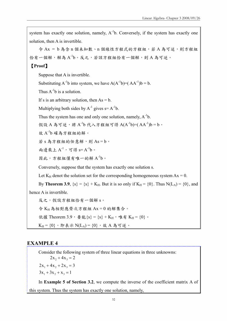
Linear Algebra- Chapter 3 20080926
32
system has exactly one solution namely A-1b Conversely if the system has exactly one
solution then A is invertible
令 Ax = b 為含 n 個未知數n 個線性方程式的方程組若 A 為可逆則方程組
恰有一個解解為 A-1b反之若該方程組恰有一個解則 A 為可逆
【Proof】
Suppose that A is invertible
Substituting A-1b into system we have A(A-1b)=( AA-1)b = b
Thus A-1b is a solution
If s is an arbitrary solution then As = b
Multiplying both sides by A-1 gives s= A-1b
Thus the system has one and only one solution namely A-1b
假設 A 為可逆將 A-1b 代入方程組可得 A(A-1b)=( AA-1)b = b
故 A-1b 確為方程組的解
若 s 為方程組的任意解則 As = b
兩邊乘上 A-1可得 s= A-1b
因此方程組僅有唯一的解 A-1b
Conversely suppose that the system has exactly one solution s
Let KH denot the solution set for the corresponding homogeneous system Ax = 0
By Theorem 39 s = s + KH But it is so only if KH = 0 Thus N(LA) = 0 and
hence A is invertible
反之假設方程組恰有一個解 s
令 KH為相對應齊次方程組 Ax = 0 的解集合
依據 Theorem 39要能s = s + KH唯有 KH = 0
KH = 0即表示 N(LA) = 0故 A 為可逆
EXAMPLE 4 Consider the following system of three linear equations in three unknowns
1xx3x33x2x4x2
2x4x2
321
321
32
=++=++
=+
In Example 5 of Section 32 we compute the inverse of the coefficient matrix A of
this system Thus the system has exactly one solution namely
Linear Algebra- Chapter 3 20080926
33
⎟⎟⎟
⎠
⎞
⎜⎜⎜
⎝
⎛=
133242420
A⎟⎟⎟
⎠
⎞
⎜⎜⎜
⎝
⎛
+minus+minus+minus+minus+
=minus
41
83
83
21
43
41
43
85
81
1A
⎟⎟⎟
⎠
⎞
⎜⎜⎜
⎝
⎛
minus+minus
=⎟⎟⎟
⎠
⎞
⎜⎜⎜
⎝
⎛
⎟⎟⎟
⎠
⎞
⎜⎜⎜
⎝
⎛
+minus+minus+minus+minus+
==⎟⎟⎟
⎠
⎞
⎜⎜⎜
⎝
⎛minus
814587
41
83
83
21
43
41
43
85
81
1
3
2
1
132
bAxxx
Theorem 311 Let Ax = b be a system of linear equations Then the system is consistent (相容)if
and only if rank(A) = rank (A∣b) Matrix (A b) is called the augmented matrix o∣ f the
system Ax = b
令 Ax = b 為線性方程式方程組則此方程組至少有一個解的『若且唯若』條件
為 rank(A) = rank (A∣b) 矩陣(A∣b)稱為方程組 Ax = b 的增廣矩陣
【Proof】
To say that Ax = b has a solution is equivalent to saying that bisinR(LA)
In the proof of Theorem 35 we saw that R(LA ) = span(a1 a2 an) the span of the
column of A
Thus Ax = b has a solution if and only if bisinspan(a1 a2 an)
But bisinspan(a1 a2 an) if and only if span(a1 a2 an) = span(a1 a2 an b)
This last statement is equivalent to
dim (span(a1a2an)) = dim (span(a1a2an b))
So by Theorem 35 the preceeding equation reduces to rank(A) = rank (A∣b)
Ax = b 有一解相當於 bisinR(LA)即 b 屬於線性轉換 LA的 Range
在 Theorem 35 的證明中提到 R(LA ) = span(a1a2an)aj 為 A 的第 j 個行
(Column)即線性轉換 LA 的 Range 係由矩陣 A 的行(Column)所生成
因此 Ax = b 要有一個解的『若且唯若』條件為 bisinspan(a1 a2 an)
至於 bisinspan(a1 a2 an)之條件
bisinspan(a1a2an) 的『若且唯若』條件為 span(a1a2an) = span(a1a2an
b)
其條件相當於
Linear Algebra- Chapter 3 20080926
34
dim (span(a1a2an)) = dim (span(a1a2an b))
依據 Theorem 35該條件可簡化為 rank(A) = rank (A∣b)
Theorem 35 The rank of any matrix equals the maximum number of its linearly
independent columns that is the rank of a matrix is the dimension of the subspace
generated by its column任一矩陣的 Rank 等於其最大線性獨立行向量數目即矩陣的
Rank 是由矩陣的行向量生成的子空間的維度【LA Fn Fm】
EXAMPLE 5 Recall the system of equations
1xx0xx
21
21
=+=+
Since ⎟⎟⎠
⎞⎜⎜⎝
⎛=
1111
A and ⎟⎟⎠
⎞⎜⎜⎝
⎛=
111011
)bA(
rank(A) = 1 and rank (A b) = 2∣
Because the two ranks are unequal the system has no solutions
矩陣 A 與增廣矩陣(A∣b) 的 Rank 不同故方程組沒有解
EXAMPLE 6 We can use Theorem 311 to determine whether (3 3 2) is in the range of the linear
transformation T R3 R3 defined by T(a1 a2 a3) = (a1+a2+a3 a1-a2+a3 a1+a3)
利用 Theorem 311 來判斷 (3 3 2)是否在線性轉換 T 的 Range 中其中T R3
R3 定義為 T(a1 a2 a3) = (a1+a2+a3 a1-a2+a3 a1+a3)
Now (3 3 2)isinR(T) if and only if there exists a vector s = x1 x2 x3 in R3 such that
T(s)=(3 3 2) Such a vector s must be a solution to the system
2xx3xxx3xxx
31
321
321
=+=+minus=++
Since the ranks of the coefficient matrix and the augmented matrix of this system
are 2 and 3 respectively it follows that this system has no solutions Hence (3 3 2) notin
R(T)
(3 3 2)isinR(T) 的『若且唯若』的條件為存在一向量 s = x1 x2 x3isinR3 使得
T(s)=(3 3 2)
Linear Algebra- Chapter 3 20080926
35
向量 s 必須是 2xx3xxx3xxx
31
321
321
=+=+minus=++
的解
因係數矩陣⎟⎟⎟
⎠
⎞
⎜⎜⎜
⎝
⎛minus
101111111
的 Rank 為 2增廣矩陣⎟⎟⎟
⎠
⎞
⎜⎜⎜
⎝
⎛minus
233
101111111
的 Rank 為 3兩
者不相等故方程組無解(3 3 2) notin R(T)
Theorem 311 Let Ax = b be a system of linear equations Then the system is consistent
(相容)if and only if rank(A) = rank (A∣b) Matrix (A b) is called the ∣ augmented
matrix of the system Ax = b 令 Ax = b 為線性方程式方程組則此方程組至少有一個
解的『若且唯若』條件為 rank(A) = rank (A∣b) 矩陣(A∣b)稱為方程組 Ax = b 的
增廣矩陣
Application
In 1973 Wassily Leontief won the Nobel prize in economics for his work in developing
a mathematical model that can be used to describe various economic phenomena
1973 年Wassily Leontief 因研究一數學模式來描述各種經濟現象而獲頒諾貝爾經
濟獎
CLOSED MODEL
We begin by considering a simple society composed of three peoples (industries) ndash a
farmer who gows all the food a tailor who makes all the clothing and a carpenter who builds
all the housing We assume that each person sells to and buy from a central pool and that
everything produced is consumed Since no commodities either enter or leave the system this
case is referred to as the CLOSE MODEL
考慮一個單純社會的三種人生產食物的農夫製衣的裁縫師與蓋住屋的木匠
並假設採取集中聯營買賣且每一件產品皆付諸消費由於過程中沒有任何成品進入
或脫離這個系統所以稱為「封閉模式」
Each of these three individual consumes all three of the commodities produced in the
Linear Algebra- Chapter 3 20080926
36
society Suppose that the proportion of each of the commodities consumed by each person is
given in the following table
社會中每一位皆消費所生產的三種成品且每一種產品也都被三位所消費其消
費比例如下
食物 Food 衣物 Clothing 住屋 Housing
農夫 Farmer 040 020 020
裁縫師 Tailor 010 070 020
木匠 Carpenter 050 010 060
Let p1 p2 and p3 denote the incomes of the farmer tailor and carpenter respectively To
ensure that this society survives we require that the consumption of each individual equals
his or her income
令 p1p2 與 p3 分別表示農夫裁縫師與木匠的收入並為確保這個封閉社會可以
存活假設每一位的收入等於消費
Note that the farmer consumes 20 of the clothing Because the total cost of all clothing
is p2 the tailorrsquos income the amount spent by the farmer on clothing is 020 p2 Moreover the
amount spent by the farmer on food clothing and housing must equal the farmerrsquos income
and so we obtain the equation 040 p1 + 020 p2 + 030 p3 = p1
對農夫而言農夫的衣物消費佔 20然因所有衣物的消費總額 p2 等於裁縫師的
收入所以農夫在衣物上的消費為 020 p2且農夫在食物衣物與住屋的總消費要等
於農夫的收入 p1所以農夫的收入與消費關係式
040 p1 + 020 p2 + 020 p3 = p1
Similary equations describing the expenditures of the tailor and carpenter produce the
following system of linear equations
同理分別對裁縫師與木匠進行討論可獲得下列方程組
Linear Algebra- Chapter 3 20080926
37
040 p1 + 020 p2 + 020 p3 = p1
010 p1 + 070 p2 + 020 p3 = p2
050 p1 + 010 p2 + 060 p3 = p3
This system can be written as Ap = p
其中⎟⎟⎟
⎠
⎞
⎜⎜⎜
⎝
⎛=
3
2
1
ppp
p 且⎟⎟⎟
⎠
⎞
⎜⎜⎜
⎝
⎛=
600100500200700100200200400
A 稱為輸入-輸出(或消費)矩陣
(Input-output (or consumption) matrix)
Ap = p 稱為均衡條件(Equilibrium condition)
能否利用不等式 p ≦ p 來替代等式
At first it may seem reasonable to replace the equilibrium condition by the inequality
Ap ≦ p that is the requirement that consumption not exceed production But in fact Ap ≦ p implies that Ap = p in the closed model
For otherwise there exists a k for which
sumgt
jjkjk pAp
Hence since the columns of A sum to 1
sumsumsumsum ==gt
jj
i jjij
ii ppAp which is a contradiction (出現矛盾)
答案是在封閉系統中Ap ≦ p Ap = p
One solution to the homogeneous system (I ndash A) x = 0 which is equivalent to the
equilibrium condition is ⎟⎟⎟
⎠
⎞
⎜⎜⎜
⎝
⎛=
400350250
p
Linear Algebra- Chapter 3 20080926
38
齊次方程組(I ndash A) x = 0 或均衡條件的一個解為 ⎟⎟⎟
⎠
⎞
⎜⎜⎜
⎝
⎛=
400350250
p
We may interpret this to mean that the society survives if the farmer taior and carpenter
have incomes in the proportions 253540
⎟⎟⎟
⎠
⎞
⎜⎜⎜
⎝
⎛=
400350250
p 可以解釋為若農夫裁縫師與木匠收入比例為 253540則社會將
能生存下去
Theorem 312
Let A be an ntimesn input-output matrix having the form ⎟⎟⎠
⎞⎜⎜⎝
⎛=
EDCB
A where D is a 1times(n-
1) positive vector and C is an (n-1)times1 positive vector Then (I-A)x = 0 has a one-
dimensional solution set that is generated by a nonnegative vector
設 A 為 ntimesn 輸入-輸出矩陣 ⎟⎟⎠
⎞⎜⎜⎝
⎛=
EDCB
A 其中D 為 1times(n-1)正向量C 為
(n-1)times1 正向量則(I-A)x = 0 具有一維解集合且該解集合係由一非負向量所生成
Any input-output matrix with all positive entries satisfies the hypothesis of this theorem
任何輸入-輸出矩陣滿足 Theorem 312 的基本假設條件例如
⎟⎟⎟
⎠
⎞
⎜⎜⎜
⎝
⎛=
02502503502500650500750
A
OPEN MODEL
In the OPEN MODEL we assume that there is an outside demand for each of the
commodities produced Returning to our simple society let x1 x2 and x3 be the monetary
values of food clothing and housing produced with respective outside demands d1 d2 and d3
Let A be the 3times3 matrix such that Aij represents the amount of commodity i required to
Linear Algebra- Chapter 3 20080926
39
produce one monetary unit of commodity j Then the value of the surplus of food in the
society is x1 ndash (A11x1+A12x2+A13x3) that is the value of food produced minus the value of
food consumed while producing the three commodities The assumption that everything
produced is consumed gives us a similar equilibrium condition for the open model namely
that the surplus of each of the three commodities must equal the corresponding outside
demands Hence i
3
1jjiji dxAx =minussum
=
for j=1 2 3
在「開放模式」中我們假設每一產品皆有外來的需求在前述的單純社會裡
令 x1x2 與 x3 分別代表食物衣物與住屋的貨幣價值d1d2 與 d3 為食物衣物與住
屋的外來需求價值令 A 為 3times3 矩陣Aij 表示生產『一個貨幣單位』的產品 j 所需要
的產品 i 的價值於是此社會中食物的盈餘價值為 x1 ndash (A11x1+A12x2+A13x3)即食物的
價值減去生產食物衣物與住屋所需消耗的食物的價值意即生產出來的食物價值扣
掉用去生產食物衣物與住屋所消耗掉的價值)(A11A12A13 為生產一個貨幣單位
的食物 1衣物 2 與住屋 3 所需消耗的食物 1 數量A12x2 表示生產貨幣價值為 x2的衣物
所需要的食物價值)對每一種產品而言其盈餘價值等於外來的需求價值於是
i
3
1jjiji dxAx =minussum
=
for j=123
Suppose that 30 cents worth of food 10 cents worth of clothing and 30 cents worth of
housing are required for the production of $1 worth of food Similar suppose that 20 cents
worth of food 40 cents worth of clothing and 20 cents worth of housing are required for the
production of $1 worth of clothing Finally suppose that 30 cents worth of food 10 cents
worth of clothing and 30 cents worth of housing are required for the production of $1 worth
of housing Then the input-output matrix is
⎟⎟⎟
⎠
⎞
⎜⎜⎜
⎝
⎛=
300200300100400100300200300
A
假設生產價值 1 元的食物需要價值 30 分的食物(A11 = 03)價值 10 分的衣物
(A21 = 01)及價值 30 分的住屋(A31 = 03)生產價值 1 元的衣物需要價值 20 分的
食物(A12 = 02)價值 40 分的衣物(A22 = 04)及價值 20 分的住屋(A32 = 02)生
Linear Algebra- Chapter 3 20080926
40
產價值 1 元的住屋需要價值 30 分的食物(A13 = 03)價值 10 分的衣物(A23 = 01)
及價值 30 分的住屋(A33 = 03)於是輸入輸出矩陣 A 為
⎟⎟⎟
⎠
⎞
⎜⎜⎜
⎝
⎛=
300200300100400100300200300
A
若食物的外來需求值為 300 億元衣物為 200 億元住屋值為 1 百億元則
⎟⎟⎟
⎠
⎞
⎜⎜⎜
⎝
⎛=
⎟⎟⎟
⎠
⎞
⎜⎜⎜
⎝
⎛
⎟⎟⎟
⎠
⎞
⎜⎜⎜
⎝
⎛
minusminusminusminusminusminus
=minus=
minus
minus
700600900
100200300
700200300100600100300200300
d)AI(x
1
1
⎟⎟⎟
⎠
⎞
⎜⎜⎜
⎝
⎛=
700600900
x 表示要滿足外來需求必須生產的食物價值為 900 億元衣物價值為
600 億元住屋價值為 700 億元
Theorem
Let AX = Y be a system of n linear equations in n variables If Andash1 exists the
solution is unique and is given by X = Andash1Y
【Proof】
Substitute X = Andash1Y into the matrix equation
AX = A(Andash1Y) = (AAndash1)Y = InY = Y
The solution is unique
Let X1 be any solution thus AX1 = Y Multiplying both sides of this equation by Andash1
gives
Andash1AX1= Andash1Y InX1 = Andash1Y X1 = Andash1Y
Linear Algebra- Chapter 3 20080926
41
Example Example 1212
2x5x3x3x5x3x21x2x x
321
321
321
minus=++minus=minusminus=minusminus
⎥⎥⎥
⎦
⎤
⎢⎢⎢
⎣
⎡
minus=
⎥⎥⎥
⎦
⎤
⎢⎢⎢
⎣
⎡
⎥⎥⎥
⎦
⎤
⎢⎢⎢
⎣
⎡
minusminusminusminusminus
231
xxx
531532211
3
2
1
Solve the system of equations
This system can be written in the following matrix form
⎥⎥⎥
⎦
⎤
⎢⎢⎢
⎣
⎡
minus⎥⎥⎥
⎦
⎤
⎢⎢⎢
⎣
⎡
minusminusminusminusminus
=
⎥⎥⎥
⎦
⎤
⎢⎢⎢
⎣
⎡minus
231
531532211
xxx 1
3
2
1
If the matrix of coefficients is invertible the unique solutionIf the matrix of coefficients is invertible the unique solution isis
Example Example 2222
1 2 1 issolution unique The 321 =minus== xxx
⎥⎥⎥
⎦
⎤
⎢⎢⎢
⎣
⎡minus=
⎥⎥⎥
⎦
⎤
⎢⎢⎢
⎣
⎡
minus⎥⎥⎥
⎦
⎤
⎢⎢⎢
⎣
⎡
minusminusminus=
⎥⎥⎥
⎦
⎤
⎢⎢⎢
⎣
⎡
121
231
123135110
xxx
3
2
1
⎥⎥⎥
⎦
⎤
⎢⎢⎢
⎣
⎡
minusminusminus=
⎥⎥⎥
⎦
⎤
⎢⎢⎢
⎣
⎡
minusminusminusminusminus
=
minus
minus
123135110
531532211
A
1
1
The The LeontiefLeontief IO Model in IO Model in Economics Economics 1515
The Leontief input-output model is used to analyze the interdependence of economics Wassily Leontief received a Nobel Prize in 1973 for his work in thie fieldThe practical applications of this model have proliferated until it has now become a standard tool for investigating economic structures ranging from cities and corporation to states and countriesConsider an economics situation that involves ninterdependent industries The output of any one industry is needed as input by other industries and even possibly by the industry itself
The The LeontiefLeontief IO Model in IO Model in Economics Economics 2525
How a mathematical model involving a system of linear equations can be constructed to analyze such a situationAssume that each industry produces one commodity Let aij denote the amount of input of a certain commodity i to produce unit output of commodity j In our model let the amounts of input and output be measured in dollars Thus for example a34 = 045 means that 45 centsrsquo worth of commodity 3 is required to produce one dollarrsquos worth of commodity 4
The The LeontiefLeontief IO Model in IO Model in Economics Economics 3535
aij = amount of commodity i in one dollar of commodity jaij =生產一元價值的j產品需要耗用的i產品價值
The elements aij called input coefficients define a matrix A called the input-output matrix which describes the interdependence of the industriesExtending the model to include an open sector (all non-producing sectors) The product of industries may go not only into other producing industries but also into other non-producing sectors of the economy such as consumers and governments
The The LeontiefLeontief IO Model in IO Model in Economics Economics 4545
di = demand of the open sectors from industry ixi=total output of industry I necessary to meet demands of all n industries and the open sector
sectoropen of demand
nindustry of demand
2industry of demand
22
1industry of demand
11
industry ofoutput total
ininii
i
i dxaxaxax ++sdotsdotsdot++=
output ofportion sectoropen
output ofportion tryinterindusoutput total
DAXX +=Demand matrixDemand matrix
Output matrixOutput matrix
The The LeontiefLeontief IO Model in IO Model in Economics Economics 5555
Applying the model to the economy of a country X Applying the model to the economy of a country X represents the total output of each of the producing sectors represents the total output of each of the producing sectors of the economy and AX describes the contributions made of the economy and AX describes the contributions made by the various sectors to fulfilling the intersectional input by the various sectors to fulfilling the intersectional input requirements of the economyrequirements of the economyD is equal to (XD is equal to (X--AX) the difference between total output AX) the difference between total output X and industry transaction AXX and industry transaction AXD is thus the gross national product of the economyD is thus the gross national product of the economy
Example Example 1414
Consider an economy consisting of three industries having Consider an economy consisting of three industries having the following inputthe following input--output matrix output matrix AA Determine the output Determine the output levels required of the industries to meet the demands of levels required of the industries to meet the demands of the other industries and of the open sector in each casethe other industries and of the open sector in each case
in turn 321812
and 896
1612
9
5100
021
21
103
51
51
⎥⎥⎦
⎤
⎢⎢⎣
⎡
⎥⎥⎦
⎤
⎢⎢⎣
⎡
⎥⎥⎦
⎤
⎢⎢⎣
⎡=
⎥⎥⎥
⎦
⎤
⎢⎢⎢
⎣
⎡
= DA
The unit of The unit of DD are millions of dollarsare millions of dollars
Linear Algebra- Chapter 3 20080926
42
Example Example 2424
We wish to compute the output levels X that correspond to We wish to compute the output levels X that correspond to the various open sector demands D X is given by the the various open sector demands D X is given by the equation X = AX + D Rewritten as followsequation X = AX + D Rewritten as follows
X ndash AX = D rArr (I ndash A)X = D rArr X = (I ndash A) ndash1 D
⎥⎥⎥
⎦
⎤
⎢⎢⎢
⎣
⎡
=⎥⎥⎥
⎦
⎤
⎢⎢⎢
⎣
⎡
minus⎥⎥⎦
⎤
⎢⎢⎣
⎡=minus minus
minusminus
5400
021
21
103
51
54
5100
021
21
103
51
31
100010001
get We AI
⎥⎥⎥
⎦
⎤
⎢⎢⎢
⎣
⎡
=minus minus
4500
038
35
85
32
35
1)( AI
output ofingcorrespond valuesvarious
4500
038
35
85
32
35
)(
401020883957522133
32816189121269
)(
1
1
DAI
DAIX
minus
minus
minusuarruarruarruarruarruarruarr
⎥⎥⎦
⎤
⎢⎢⎣
⎡=
⎥⎥⎦
⎤
⎢⎢⎣
⎡
⎥⎥⎥
⎦
⎤
⎢⎢⎢
⎣
⎡
=minus=
Example Example 3434
By using Gauss-Jordan elimination
dollars of milliond are units The
40
15674
and 106629
209946
are 321812
and 896
1612
9
⎥⎥⎥
⎦
⎤
⎢⎢⎢
⎣
⎡
⎥⎥⎥
⎦
⎤
⎢⎢⎢
⎣
⎡
⎥⎥⎥
⎦
⎤
⎢⎢⎢
⎣
⎡
⎥⎥⎥
⎦
⎤
⎢⎢⎢
⎣
⎡
⎥⎥⎥
⎦
⎤
⎢⎢⎢
⎣
⎡
⎥⎥⎥
⎦
⎤
⎢⎢⎢
⎣
⎡
Example Example 4444
The output levels necessary to meet the demandsThe output levels necessary to meet the demands
IAAAIAI m =++++minus ))(( 2 L
mAAAIAI ++++=minus minus L21)(
Computing (IComputing (I--A) A) --11
1m
m2m2
m2
AI)AAAI(A)AAAI(I
)AAAI)(AI(
+minus=++++minus++++=
++++minusLL
L
NOTE 0A 1m rarr+
Population Movement Population Movement 1313
In 2000 58 million of people live in cities and 142 million of In 2000 58 million of people live in cities and 142 million of people people live in the surrounding suburbs Represent this information by tlive in the surrounding suburbs Represent this information by the he matrix matrix
The probability of a person staying in the city was 096 Thus tThe probability of a person staying in the city was 096 Thus the he probability of moving to the suburbs was 004 probability of moving to the suburbs was 004 The probability of a person moving to the city was 001 the The probability of a person moving to the city was 001 the probability of remaining in suburbia was 099probability of remaining in suburbia was 099
suburbcity
990040010960
suburbcity (to))from(
⎥⎦
⎤⎢⎣
⎡=P
⎥⎦
⎤⎢⎣
⎡=
14258
X0
City population in 2001 = people who remained from 2000 + peopleCity population in 2001 = people who remained from 2000 + peoplewho moved in from the suburbs = ( 096 who moved in from the suburbs = ( 096 timestimes 58 ) + (001 58 ) + (001 timestimes 142 ) = 142 ) = 571 million571 millionSuburban population in 2001 = people who moved in from the city Suburban population in 2001 = people who moved in from the city + people who stayed from 2000 = ( 004 + people who stayed from 2000 = ( 004 timestimes 58 ) + (099 58 ) + (099 timestimes 142 ) = 142 ) = 1429 million1429 millionCan arrive at these numbers using matrix multiplicationCan arrive at these numbers using matrix multiplication
⎥⎦
⎤⎢⎣
⎡=⎥
⎦
⎤⎢⎣
⎡⎥⎦
⎤⎢⎣
⎡==
9142157
14258
990040010960
PXX 01
Population Movement Population Movement 2323
Population Movement Population Movement 3333
Assume that the population flow represented by the matrix P is unchanged over the years The population distribution X2 after 2 years is given by X2 = P X1 = P2 X0 In general
Pn is called the n-step transition matrix The (ij)th element of Pngives the probability of going from state j to state i in n stepsFor example
in
ni XPX =+
suburbcity
960150040850
P
suburbcity (to))from(
4
⎥⎦
⎤⎢⎣
⎡=
The probability of living in the city in The probability of living in the city in 2000 and being in the suburbs 4 years 2000 and being in the suburbs 4 years later is 015later is 015
Markov ChainsMarkov Chains
The probabilities in the above model depend only on the The probabilities in the above model depend only on the current state of a person whether the person is living in the current state of a person whether the person is living in the city or in suburbiacity or in suburbiaThis type of model in which the probability of going from This type of model in which the probability of going from one state to another depends only on the current state one state to another depends only on the current state rather than on a more complete historical description is rather than on a more complete historical description is called a called a Markov chainMarkov chainMarkov chains are useful tools for scientists in many Markov chains are useful tools for scientists in many fields such as geneticsfields such as genetics
Linear Algebra- Chapter 3 20080926
43
GeneticsGenetics 1414
Genetics is the branch of biology that deals with Genetics is the branch of biology that deals with heredity heredity (遺傳)(遺傳) It is the study of units called It is the study of units called genes which determine the characteristics living genes which determine the characteristics living things inherit from their parents The inheritance things inherit from their parents The inheritance (遺傳)(遺傳)of such traitsof such traits(特徵)(特徵)as sex height eye as sex height eye color and hair color of human beings and such color and hair color of human beings and such traits as petaltraits as petal(花瓣)(花瓣) color and leaf shape of color and leaf shape of plants are governed by genesplants are governed by genesIn medicine agricultureIn medicine agriculturehelliphellip
GeneticsGenetics 2424
The traits of guinea pigsThe traits of guinea pigs(天竺鼠)(天竺鼠)are long hair and short hairare long hair and short hairThe length of hair is governed by a pair of gene which we denoteThe length of hair is governed by a pair of gene which we denote A A and aand aA guinea pig may have any one of the combination of AA A guinea pig may have any one of the combination of AA AaAa or or aaaa Each of these classes is called a genotypeEach of these classes is called a genotype(基因型)(基因型)The AA type guinea pig is indistinguishable in appearance from tThe AA type guinea pig is indistinguishable in appearance from the he AaAa type type ndashndash both have long hair both have long hair ndashndash whereas the whereas the aaaa type has short hairtype has short hairThe A gene is said to dominate the a geneThe A gene is said to dominate the a geneAn animal is called dominant An animal is called dominant (顯性)(顯性)if it has AA genes hybridif it has AA genes hybrid(混種)(混種) with with AaAa genes and recessive genes and recessive (隱性)(隱性)with with aaaa genesgenes
GeneticsGenetics 3434
When two guinea pigs are crossed the offspring inherits one genWhen two guinea pigs are crossed the offspring inherits one gene e from each parent in random mannerfrom each parent in random mannerGiven the genotype of the parents we can determine the Given the genotype of the parents we can determine the probabilities of the genotype of the offspringprobabilities of the genotype of the offspring
AA+AA AA+AA probabilities of AA probabilities of AA AaAa and and aaaa are 10and 0are 10and 0Aa+AAAa+AA probabilities of AA probabilities of AA AaAa and and aaaa are are frac12frac12 frac12frac12 and 0 and 0aa+AAaa+AA probabilities of AA probabilities of AA AaAa and and aaaa are 0 1 and 0are 0 1 and 0
This series of experiments is a Markov chain having transition This series of experiments is a Markov chain having transition matrixmatrix
aaAaAA
00012100211
P
aaAaAA
⎥⎥⎥
⎦
⎤
⎢⎢⎢
⎣
⎡=
GeneticsGenetics 4444
Assume an initial population of guinea pigs made up of an Assume an initial population of guinea pigs made up of an equal number of each genotypeequal number of each genotype
⎥⎥⎥
⎦
⎤
⎢⎢⎢
⎣
⎡=
313131
X0
The fractions of following generations are
⎥⎥⎥
⎦
⎤
⎢⎢⎢
⎣
⎡=
⎥⎥⎥
⎦
⎤
⎢⎢⎢
⎣
⎡=
⎥⎥⎥
⎦
⎤
⎢⎢⎢
⎣
⎡=
⎥⎥⎥
⎦
⎤
⎢⎢⎢
⎣
⎡=
01611615
X08187
X04143
X02121
X 4321
AAAAAaAaaaaa
3-4 Systems of Linear Equations ndash Computational Aspects
DEFINITION 36 Equivalent
Two systems of linear equations are called equivalent if they have the same solution
set
兩個線性方程組稱為等價意指兩者具有相同的解集合
Elementary Transformations Transformation called elementary transformations can be used to change a system of
linear equations into another system of linear equations that have the same solution
These transformations are used to solve system of linear equations by eliminating
variables
The equivalent transformations used in terms of matrix are called ELEMENTARY
ROW OPERATION
Linear Algebra- Chapter 3 20080926
44
Equivalent System Systems of equations that are related through elementary transformations are called
equivalent systems
Matrices that are related through elementary row operations are called row equivalent
matrices
The symbol asymp is used to indicate equivalence in both cases
Theorem 313 Let Ax = b be a system of m linear equations in n unknowns and let C be an invertible
mtimesm matrix Then the system (CA)x = Cb is equivalent to Ax = b
設 Ax = b 為含 n 個未知數m 個線性方程式的方程組若 C 為可逆的mtimesm
矩陣則(CA)x = Cb 等價於 Ax = b
【Proof】
Let K be the solution set for Ax = b and Krsquo the solution set for (CA)x = Cb If wisinK
then Aw = b So (CA)w = Cb and hence wisinKrsquo Thus KsubeKrsquo
Conversely if wisinKrsquo then (CA)w = Cb Hence Aw = C-1(CA)w = C-1(Cb) = b so
wisinK Thus KrsquosubeK and therefore K=Krsquo
設 K 為 Ax = b 的解集合且 Krsquo為(CA)x = Cb 的解集合
若 wisinK則 Aw = b (CA)w = Cb故 wisinKrsquo於是 KsubeKrsquo
反之若 wisinKrsquo則(CA)w = Cb Aw = C-1(CA)w = C-1(Cb) = b故 wisinK於是
KrsquosubeK因此K=Krsquo
Corollary Let Ax = b be a system of m linear equations in n unknowns If (Arsquo brsquo) is obtained ∣
from from (A b) by a finite number of elementary row operations then the system Arsquox = ∣
brsquo is equivalent to the original system
設 Ax = b 為含 n 個未知數m 個線性方程式的方程組若(Arsquo brsquo) ∣ 是由(A b) ∣
經過有限次數的基本列運算而得則 Arsquox = brsquo 等價於 Ax = b即兩者具有相同的解
集合
【Proof】
Suppose that (Arsquo brsquo) is obtained from (A b) by elementary row operations These ∣ ∣
Linear Algebra- Chapter 3 20080926
45
may be executed by multiplying (A b) by elementary mtimesm matrices E∣ 1 E2hellipEp Let
C=EphellipE2E1 then (Arsquo brsquo) = C(A b) = (CA Cb)∣ ∣ ∣
Since each Ei is invertible so is C Now Arsquo = CA and brsquo = Cb Thus by Theorem 313
the system Arsquox = brsquo is equivalent to the system Ax = b
設(Arsquo brsquo)∣ 是由(A b)∣ 經過基本列運算取得即以基本 mtimesm 矩陣 E1 E2hellipEp
乘上 (A b)∣ (Arsquo brsquo) = C(A b) = (CA Cb∣ ∣ ∣ )其中C=EphellipE2E1
因 Ei 可逆故 C 亦為可逆 Arsquo = CA 且 brsquo = Cb
依據 Theorem 313Arsquox = brsquo 等價於 Ax = b
Theorem 313 Let Ax = b be a system of m linear equations in n unknowns and let C be an
invertible mtimesm matrix Then the system (CA)x = Cb is equivalent to Ax = b 設 Ax = b
為含 n 個未知數m 個線性方程式的方程組若 C 為可逆的mtimesm 矩陣則(CA)x
= Cb 等價於 Ax = b
We now describe a method for solving any stystem of linear equations Consider for
example the system of linear equations
探討解線性方程組的方法hellip
2xxx2x3xxx1x2x3x2x3
4321
321
4321
=minus++=++=minus++
First we form the augmented matrix ⎟⎟⎟
⎠
⎞
⎜⎜⎜
⎝
⎛
minus
minus
231
112101112323
(增廣矩陣)
Interchanging the first and third rows ⎟⎟⎟
⎠
⎞
⎜⎜⎜
⎝
⎛
minus
minus
132
132301111121
(第 13 列互調)
Adding -1 times the first row to the second row and then add -3 times the first row to
the third row ⎟⎟⎟
⎠
⎞
⎜⎜⎜
⎝
⎛
minusminusminus
minus
512
104010101121
(第 1 列乘上 -1 加到第 2 列再以 -3 乘上
第 1 列加到第 3 列)
Linear Algebra- Chapter 3 20080926
46
Multiplying the second row by -1 ⎟⎟⎟
⎠
⎞
⎜⎜⎜
⎝
⎛
minusminus
minusminusminus
51
2
104010101121
(第 2 列乘上 -1)
Adding four times the second row to the third row ⎟⎟⎟
⎠
⎞
⎜⎜⎜
⎝
⎛
minusminus
minusminusminus
91
2
300010101121
(4 乘上第 2
列加到第 3 列)
Multiplying the third row by -13 ⎟⎟⎟
⎠
⎞
⎜⎜⎜
⎝
⎛minusminus
minus
31
2
100010101121
(第 3 列乘上 -13)
Adding the third row to the first and second rows to obtain zeros in row 1 column 4
and row 2 column 4 ⎟⎟⎟
⎠
⎞
⎜⎜⎜
⎝
⎛
325
100000100121
(將第 3 列加到第 1 列及第 2 列)
Adding -2 times the second row to the first row in order to make the first row second
column entry become zero ⎟⎟⎟
⎠
⎞
⎜⎜⎜
⎝
⎛
321
100000100101
(將第 2 列乘以 -2 再加至第 1 列)
We have now obtained the desired reduction of the augmented matrix
⎟⎟⎟
⎠
⎞
⎜⎜⎜
⎝
⎛
321
100000100101
是化簡後的增廣矩陣
This matrix corresponds to the system of linear equations
對應的線性方程組為
2x3x1xx
4
2
31
===+
By Corollary to Theorem 313 this system is equivalent to the original system But this
system is easily solved Obviously x2 = 2 and x4 = 3 Moreover x1 and x3 can be any values
Linear Algebra- Chapter 3 20080926
47
provided their sum is 1 Letting x3 = t we then have x1 = 1 ndash t Thus an arbitray solution to the
original system has the form
依據 Corollary to Theorem 313 化簡後的方程組與原方程組等值此方程組的解為
x2 = 3x4 = 3x1 + x3 = 1於是原方程組的任意解可以寫成
⎟⎟⎟⎟⎟
⎠
⎞
⎜⎜⎜⎜⎜
⎝
⎛minus
+
⎟⎟⎟⎟⎟
⎠
⎞
⎜⎜⎜⎜⎜
⎝
⎛
=
⎟⎟⎟⎟⎟
⎠
⎞
⎜⎜⎜⎜⎜
⎝
⎛ minus
0101
t
3021
3t2
t1
Observe that
⎪⎪⎭
⎪⎪⎬
⎫
⎪⎪⎩
⎪⎪⎨
⎧
⎟⎟⎟⎟⎟
⎠
⎞
⎜⎜⎜⎜⎜
⎝
⎛minus
0101
is a basis for the homogeneous system of equations
corresponding to the given system
其中
⎪⎪⎭
⎪⎪⎬
⎫
⎪⎪⎩
⎪⎪⎨
⎧
⎟⎟⎟⎟⎟
⎠
⎞
⎜⎜⎜⎜⎜
⎝
⎛minus
0101
是齊次方程組解集合的一組基底
Gauss-Jordan Elimination
Let A be an n times n matrix
1 Adjoin the identity n times n matrix In to A to form the matrix [A In]
2 Compute the reduced echelon form of [A In]
(1) If the reduced echelon form is of the type [In B] then B is the inverse of A
(2) If the reduced echelon form is not of the type [In B] in that the first n times n
submatrix is not In then A has no inverse
An n times n matrix A is invertible if and only if its reduced echelon form is In
DEFINITION 37 Reduced Row Echelon Form
A matrix is said to be in reduced row echelon form if the following three conditions
are satisfied
Linear Algebra- Chapter 3 20080926
48
一個矩陣可以被稱為簡約列梯形式必須具備有下列三條件
(a) Any row containing a nonzero entry preceeds any row in which all the entries are
zero (if any)
含有非零元素的任一列排在全含零元素的任一列前面(儘可能)
(b) The first nonzero entry in each row in the only nonzero entry in its column
各列中第一個非零元素為其所在行中唯一的非零元素
(c) The first nonzero entry in each row is 1 and it occurs in a column to thr right of the
first nonzero entry in the preceeding row
各列中第一個非零元素為 1 且它出現在前一列中第一個非零元素的右邊某一
行中
Reduced Echelon Form A matrix is in reduced echelon form if
1 Any rows consisting entirely of zeros are grouped at the bottom of the matrix
2 The first nonzero element of each other row is 1 This element is called a leading 1
3 The leading 1 of each row after the first is positioned to the right of the leading 1 of
the previous row
4 All other elements in a column that contains a leading 1 are zero
Theorem 314 Gaussian Elimination Transformation Gaussian elimination transform any matrix into its reduced row echelon form
利用 Gaussian elimination 將矩陣轉換成簡約列梯形式
We now describe a method for solving a system in which the augmented matrix is in
reduced row echelon form To illustrate this procedure we consider the system
14x8x3x2x2x28x5x2xxx6x3xxxx17x9x4xx3x2
54321
54321
54321
54321
=minus+++=minus+++=minus+++=minus+++
Linear Algebra- Chapter 3 20080926
49
for which the augmented matrix is
⎟⎟⎟⎟⎟
⎠
⎞
⎜⎜⎜⎜⎜
⎝
⎛
minusminusminusminus
1486
17
83222521113111194132
(增廣矩陣)
Applying Gaussian elimination to the augmented matrix of the system produces the
following sequence of matrices
利用 Gaussian elimination method 處理增廣矩陣
⎟⎟⎟⎟⎟
⎠
⎞
⎜⎜⎜⎜⎜
⎝
⎛
minusminusminusminus
1486
17
83222521113111194132
⎟⎟⎟⎟⎟
⎠
⎞
⎜⎜⎜⎜⎜
⎝
⎛
minusminusminusminus
148
176
83222521119413231111
⎟⎟⎟⎟⎟
⎠
⎞
⎜⎜⎜⎜⎜
⎝
⎛
minusminus
minus
0213
0000021000
1011020201
The system of linear equations corresponding to thus last matrix is
對應最後矩陣的線性方程組 2x2x
1xxx3x2x2x
54
532
531
=minus=+minus=minus+
Assign x3 = t1 x5 = t2
2t22x2x1tt1xxx
3t2t23x2x2x
254
21532
21531
+=+=+minus=+minus=
++minus=++minus=
Thus an arbitray solution s is of the form
於是任意解 s 具有下列形式
s =
⎟⎟⎟⎟⎟⎟
⎠
⎞
⎜⎜⎜⎜⎜⎜
⎝
⎛minus
+
⎟⎟⎟⎟⎟⎟
⎠
⎞
⎜⎜⎜⎜⎜⎜
⎝
⎛minus
+
⎟⎟⎟⎟⎟⎟
⎠
⎞
⎜⎜⎜⎜⎜⎜
⎝
⎛
=
⎟⎟⎟⎟⎟⎟
⎠
⎞
⎜⎜⎜⎜⎜⎜
⎝
⎛
+
+minus++minus
=
⎟⎟⎟⎟⎟⎟
⎠
⎞
⎜⎜⎜⎜⎜⎜
⎝
⎛
1201
2
t
00112
t
02013
t2t2
t1tt
3t2t2
xxxxx
21
2
2
1
21
21
5
4
3
2
1
where t1t2isinR
Linear Algebra- Chapter 3 20080926
50
Notice that
⎪⎪⎪
⎭
⎪⎪⎪
⎬
⎫
⎪⎪⎪
⎩
⎪⎪⎪
⎨
⎧
⎟⎟⎟⎟⎟⎟
⎠
⎞
⎜⎜⎜⎜⎜⎜
⎝
⎛minus
⎟⎟⎟⎟⎟⎟
⎠
⎞
⎜⎜⎜⎜⎜⎜
⎝
⎛minus
1201
2
00112
is a basis for the solution set of the corresponding
homogeneous system of equation and
⎟⎟⎟⎟⎟⎟
⎠
⎞
⎜⎜⎜⎜⎜⎜
⎝
⎛
02013
is a particular solution to the original system
⎪⎪⎪
⎭
⎪⎪⎪
⎬
⎫
⎪⎪⎪
⎩
⎪⎪⎪
⎨
⎧
⎟⎟⎟⎟⎟⎟
⎠
⎞
⎜⎜⎜⎜⎜⎜
⎝
⎛minus
⎟⎟⎟⎟⎟⎟
⎠
⎞
⎜⎜⎜⎜⎜⎜
⎝
⎛minus
1201
2
00112
是齊次方程組解集合的一組基底
⎟⎟⎟⎟⎟⎟
⎠
⎞
⎜⎜⎜⎜⎜⎜
⎝
⎛
02013
是原方程組的特別解
EXAMPLE 1
The matrix ⎟⎟⎟
⎠
⎞
⎜⎜⎜
⎝
⎛
101010011
is not in reduced row echelon form
因為第一行含有第一個非零元素在第一列但第一行尚含有其他非零元素
The matrix ⎟⎟⎟
⎠
⎞
⎜⎜⎜
⎝
⎛
110010012010
is not in reduced row echelon form
因為第一列第一個非零元素不在第一列第一個非零元素的右邊
The matrix ⎟⎟⎠
⎞⎜⎜⎝
⎛010002
is not in reduced row echelon form
因為第一列的第一個非零元素不是 1
Linear Algebra- Chapter 3 20080926
51
Reduced Echelon FormReduced Echelon Form
⎥⎥⎥
⎦
⎤
⎢⎢⎢
⎣
⎡
910030107001
⎥⎥⎥
⎦
⎤
⎢⎢⎢
⎣
⎡
100001000041
⎥⎥⎥
⎦
⎤
⎢⎢⎢
⎣
⎡
000210801
Not in Reduced Echelon Form
⎥⎥⎥
⎦
⎤
⎢⎢⎢
⎣
⎡
310000004021
⎥⎥⎥
⎦
⎤
⎢⎢⎢
⎣
⎡
100000430003021
⎥⎥⎥⎥
⎦
⎤
⎢⎢⎢⎢
⎣
⎡
0000210030108071
In Reduced Echelon Form
Use GaussUse Gauss--Jordan elimination to Jordan elimination to find reduced echelon formfind reduced echelon form 1313
Step 1 Interchange rows if necessary to bring a nonzero Step 1 Interchange rows if necessary to bring a nonzero element to the top of the first nonzero column This nonzero element to the top of the first nonzero column This nonzero element is called a pivotelement is called a pivot
⎥⎥⎦
⎤
⎢⎢⎣
⎡
minusminus
minus
1211244129333
22200
⎥⎥⎥
⎦
⎤
⎢⎢⎢
⎣
⎡
minusminus
minus
harrasymp
121124422200
129333
R2R1
Use GaussUse Gauss--Jordan elimination to Jordan elimination to find reduced echelon formfind reduced echelon form 2323
Step 2 Create a 1 in the pivot location by multiplying the Step 2 Create a 1 in the pivot location by multiplying the pivot row by 1pivotpivot row by 1pivot
Step 3 Create zero elsewhere in the pivot column by adding Step 3 Create zero elsewhere in the pivot column by adding suitable multiples of the pivot row to all other rows of the suitable multiples of the pivot row to all other rows of the matrixmatrix
⎥⎥⎥
⎦
⎤
⎢⎢⎢
⎣
⎡
minusminusminus
minus
minus+asymp
412002220043111
4)R1(R3
⎥⎥⎦
⎤
⎢⎢⎣
⎡
minusminus
minus
⎟⎠⎞
⎜⎝⎛asymp
12112442220043111
R13
1
The matrix is the reduced echelon form of the given matrixThe matrix is the reduced echelon form of the given matrix
Use GaussUse Gauss--Jordan elimination to Jordan elimination to find reduced echelon formfind reduced echelon form 3333
Step 4 Cover the pivot row and all rows above it Repeat Steps Step 4 Cover the pivot row and all rows above it Repeat Steps 1 1 and 2 for the remaining and 2 for the remaining submatrixsubmatrix Repeat Step 3 for the whole Repeat Step 3 for the whole matrix Continue until the reduced echelon form is reachedmatrix Continue until the reduced echelon form is reached
⎥⎥⎥
⎦
⎤
⎢⎢⎢
⎣
⎡
minusminus
+minus+asymp
⎥⎥⎥
⎦
⎤
⎢⎢⎢
⎣
⎡
minusminus
minus++asymp
⎥⎥⎥
⎦
⎤
⎢⎢⎢
⎣
⎡
minusminusminus
minus
⎟⎠⎞
⎜⎝⎛
asymp
⎥⎥⎥
⎦
⎤
⎢⎢⎢
⎣
⎡
minusminusminus
minus
6100050100
170011
R3R22)R3(R1
610001110052011
R2)2(R3R2R1
412001110043111
R221
412002220043111
Theorem 315 Let Ax = b be a system of r nonzero equations is in n unknown Suppose that rank(A)
= rank (A b)∣ and that (A b)∣ is in reduced row echelon form Then
設 Ax = b 為含有 n 個未知數r 個非零方程式的方程組假設 rank(A) = rank
(A b)∣ 且 (A b)∣ 為簡約列梯形式於是
(a) rank(A) = r
(b) If the general solution obtained by the procedure above is of the form s = s0 + t1u1
+ t2u2 +hellip+ tn-run-r then u1 u2hellip un-r is a basis for the solution set of the
corresponding homogeneous system and s0 is a solution to the original system 由
前述方法所得的 General solution 具有下列形式
s = s0 + t1u1 + t2u2 +hellip+ tn-run-r
其中u1 u2hellip un-r為齊次方程組 Ax = 0 的解集合的一組基底且 s0 為原方
程組的一個解)
【Proof】
Since (A b)∣ is in reduced row echelon form (A b)∣ must have r nonzero rows
Clearly these rows are linearly independent by the definition of the reduced row echelon
Linear Algebra- Chapter 3 20080926
52
form and so rank (A b)∣ = r Thus rank(A) = r
Let K be the solution set for Ax = b and let KH be the solution set for Ax = 0 Setting
t1 = t2 =hellip= tn-r = 0 we see that s = s0isinK But by Theorem 39 K = s +KH Hence
KH = - s0+K = span(u1 u2hellip un-r )
Because rank(A) = r we have dim(KH) = n-r Thus since dim(KH) = n-r and KH is
generated by a set u1 u2hellip un-r containing at most n-r vectors that is a basis for KH
由於(A b)∣ 具有簡約列梯形式因此(A b)∣ 必定具有 r 個非零列由簡約列梯形
式的定義得知 r 個非零列為線性獨立故 rank (A b)∣ = rrank(A) = r
令 K 為 Ax = b 的解集合 KH 為 Ax = 0 的解集合
假設 t1 = t2 =hellip= tn-r = 0(u1 u2hellip un-r非 KH的基底)則 s = s0isinK
依據 Theorem 39K = s +KH KH = - s0+K = span(u1 u2hellip un-r )
因 rank(A) = r所以 dim(KH) = n - r 且 KH 是由u1 u2hellip un-r 所生成
故原假設「t1 = t2 =hellip= tn-r = 0」不成立
因此 KH含有最多 n - r 個向量且這些向量為 KH的基底
Theorem 39 Let K be the solution set of a system of linear equations Ax = b and let KH be
the solution set of the corresponding homogeneous system Ax = 0 Then for any solution s
to Ax = b K =s + KH = s+k kisinKH 設 K 為線性方程組 Ax = b 的解集合且 KH
為對應的齊次方程組的解集合則對 Ax = b 的任一個解 s 而言K =s + KH = s+k
kisinKH
ExampleExampleSolve the system of equationsSolve the system of equations
7537429333
321
321
321
=minusminus=+minus=+minus
xxxxxxxxx
⎥⎥⎦
⎤
⎢⎢⎣
⎡
++asymp
000012104301
R2R3R2R1 12
431243
32
31
32
31+minus=+minus=rArr=+
=+rArr xxxx
xxxx
The general solution to the system isThe general solution to the system is
parameter) a (callednumber real is where 1243
3
2
1
rrxrxrx
=+minus=+minus=
⎥⎥⎥
⎦
⎤
⎢⎢⎢
⎣
⎡
minusminusminus
minus
minus+minus+asymp
⎥⎥⎥
⎦
⎤
⎢⎢⎢
⎣
⎡
minusminusminusminus
asymp
⎥⎥⎥
⎦
⎤
⎢⎢⎢
⎣
⎡
minusminusminusminus
242012103111
1R)3(3R1R)2(2R
715374123111
715374129333
R131
ExampleExample
Solve the system of equationsSolve the system of equations446942
1423258101242
4321
4321
4321
=minus+minusminus=+minus+minus
=minus+minus
xxxxxxxxxxxx
⎪⎪
⎩
⎪⎪
⎨
⎧
===
minus=
rArr==minus=minus
rArr
1x6xrx
2r2x
1x6x
2x2x
4
3
2
1
4
3
21
⎥⎥⎥
⎦
⎤
⎢⎢⎢
⎣
⎡ minusminusasymp
⎥⎥⎥
⎦
⎤
⎢⎢⎢
⎣
⎡minus
minusminusasymp
⎥⎥⎥
⎦
⎤
⎢⎢⎢
⎣
⎡
minusminusminusminusminusasymp
⎥⎥⎥
⎦
⎤
⎢⎢⎢
⎣
⎡
minusminusminusminusminusasymp
⎥⎥⎥
⎦
⎤
⎢⎢⎢
⎣
⎡
minusminusminusminusminus
minusminusasymp
⎥⎥⎥
⎦
⎤
⎢⎢⎢
⎣
⎡
minusminusminusminusminus
minusminus
+
minus+
+
minus+
minus+
+
110006010020021
110005110011021
14430051100
295621
2R31
144300153300295621
446942142321295621
44694214232158101242
R3R2
1)R3(R1
3R2R3
6)R2(R1
2)R1(R3
R1R2R1
21
Linear Algebra- Chapter 3 20080926
53
ExampleExampleSolve the system of equationsSolve the system of equations
432636242232
54321
54321
54321
=+minus+minusminus=++minus+=++minus+
xxxxxxxxxxxxxxx
⎥⎥⎦
⎤
⎢⎢⎣
⎡ minusasymp
⎥⎥⎦
⎤
⎢⎢⎣
⎡
minusminusminusminusminus
+
minus+
642000210000213121
431121636242213121
R1R3
2)R1(R2
⎥⎥⎦
⎤
⎢⎢⎣
⎡ minusasympharr 210000
642000213121
R3R2 ( ) ⎥⎥⎦
⎤
⎢⎢⎣
⎡ minusasymp
210000321000213121
2R21
⎥⎥⎦
⎤
⎢⎢⎣
⎡ minusminusminusasympminus+ 210000
321000750121
3)R2(R1 ⎥⎥⎦
⎤
⎢⎢⎣
⎡minus
minusasymp
minus+
+
210000101000300121
2)R3(R2
5R3R1
2x1x
3xx2x
5
4
321
=minus=
++minus=rArr
2xs and r somefor 1x sx rx
3sr2x
5
432
1
=minus===
++minus=
ExampleExample
Solve the system of Solve the system of equationsequations 122
32452232
32
321
321
321
=+minus=minus+
=+minus=+minus
xxxxxxxxxxx
⎥⎥
⎦
⎤
⎢⎢
⎣
⎡asymp
minusminusminus
minus
harr1220210063303211
R3R2
( ) ⎥⎥
⎦
⎤
⎢⎢
⎣
⎡asymp
minusminusminus
minus
1220210021103211
R231
⎥⎥
⎦
⎤
⎢⎢
⎣
⎡asympminusminusminus
minus+
+
5400210021101101
2)R2(R4
R2R1 ⎥⎥
⎦
⎤
⎢⎢
⎣
⎡asymp
minusminus
minus+
+
minus+
13000210040103001
4)R3R(R4
R3R2
1)R3(R1
( ) ⎥⎥
⎦
⎤
⎢⎢
⎣
⎡asymp
minusminus
1000210040103001
R4131
The system has no solutionThe system has no solution
⎥⎥
⎦
⎤
⎢⎢
⎣
⎡asymp
⎥⎥
⎦
⎤
⎢⎢
⎣
⎡
minusminusminus
minus
minusminusminusminus
minus+
minus+
1220633021003211
1220312145223211
1)R1(R3
2)R1(R2
0x1+0x2+0x3=1
Curve FittingCurve Fitting
A set of data points A set of data points is given and it is is given and it is necessary to find a polynomial whose graph passes through the necessary to find a polynomial whose graph passes through the points points The points are often measurements in an experiment The points are often measurements in an experiment The xThe x--coordinates are called coordinates are called base pointsbase pointsIt can be shown that if the base points are all distinct then aIt can be shown that if the base points are all distinct then a unique unique polynomial of degree n polynomial of degree n ndashndash 1 (or less)1 (or less)
can be fitted to thecan be fitted to the pointspoints
) ( ) ( ) ( 2211 nn yxyxyx K
11
2210
minusminus
minusminus ++++= n
nn
n xaxaxaay K
The coefficients can be found by substituting the points The coefficients can be found by substituting the points into the polynomial equation and then solving a system into the polynomial equation and then solving a system of linear equationsof linear equations
ExampleExample
Determine the equation of the polynomial of degree 2 whose graphpasses through the points (1 6) (2 3) (3 2)
Let the polynomial be and substituting x = 1 y = 6 x = 2 y = 3 x = 3 y = 2 we have
Solving this system for a0 a1 and a2 using Gauss-Jordan elimination
⎥⎥⎥
⎦
⎤
⎢⎢⎢
⎣
⎡minus
minus
minus+minus+asymp
220033109201
1)R2(R31)R2(R1
2210 xaxaay ++=
2a9a3a3a4a2a6aaa
210
210
210
=++=++=++
⎥⎥⎥
⎦
⎤
⎢⎢⎢
⎣
⎡
minusminus
⎥⎥⎥
⎦
⎤
⎢⎢⎢
⎣
⎡
minus+minus+asymp
482033106111
293134216111
1)R1(R31)R1(R2
( )⎥⎥⎥
⎦
⎤
⎢⎢⎢
⎣
⎡minus
⎥⎥⎥
⎦
⎤
⎢⎢⎢
⎣
⎡minus
minusasymp
minus++asymp
11006010
11001
110033109201
3)R3(R22R3R1
R321
We get a0 = 11 a1 = ndash 6 a2 = 1The parabola that passes through these points is y = 11 ndash 6x + x2
ExampleExample Traffic FlowTraffic Flow
Network analysis plays an important role in electrical Network analysis plays an important role in electrical engineeringengineeringThe concepts and tools of network analysis have been The concepts and tools of network analysis have been found to be useful in many other fields such as found to be useful in many other fields such as information theory and the study of transportation systemsinformation theory and the study of transportation systemsThe analysis of traffic flow through a road network during The analysis of traffic flow through a road network during peak period illustrates how systems of linear equations peak period illustrates how systems of linear equations with with manymany solutions can arise in practicesolutions can arise in practice
Traffic FlowTraffic Flow
Consider the typical road network The streets are all oneConsider the typical road network The streets are all one--way with the arrows indicating the direction of traffic flowway with the arrows indicating the direction of traffic flowThe flow of traffic in and out of the network is measured The flow of traffic in and out of the network is measured in vehicles per hour (in vehicles per hour (vphvph))How to construct a mathematical model to analyze this How to construct a mathematical model to analyze this network network
Traffic Traffic FlowFlowTRAFFIC LAWTRAFFIC LAWhelliphellipAll traffic entering an intersection must leave that All traffic entering an intersection must leave that intersectionintersection
Linear Algebra- Chapter 3 20080926
54
Junction AJunction BJunction CJunction DJunction EJunction F 600
800 200 500 100 600
54
643
73
72
621
51
=+=++minus=+minus=minus=+minus=+
xxxxx
xxxx
xxxxx
⎥⎥⎥⎥⎥⎥⎥⎥⎥⎥⎥⎥⎥
⎦
⎤
⎢⎢⎢⎢⎢⎢⎢⎢⎢⎢⎢⎢⎢
⎣
⎡
asympasymp
⎥⎥⎥⎥⎥⎥⎥⎥⎥⎥⎥⎥⎥
⎦
⎤
⎢⎢⎢⎢⎢⎢⎢⎢⎢⎢⎢⎢⎢
⎣
⎡
minusminus
minusminusminusminus
minusminus
minusminus
0000000001110000
6001101000200100010050010000106001100001
600001100080001011002001000100500100001010001000116000010001
L
Traffic FlowTraffic FlowJunction AJunction BJunction CJunction DJunction EJunction F 600
800 200 500 100 600
54
643
73
72
621
51
=+=++minus=+minus=minus=+minus=+
xxxxx
xxxx
xxxxx
Perform road work on x7 Because x3 ge 0 the minimum flow 200 in the branch x7 can be obtained by making x3 = 0 (closing DE to traffic)
Traffic FlowTraffic Flow
We get
765
76473
72761
xx x600xxx200x x500x x600xxx
minus=++minus=minus=+=+minusminus=
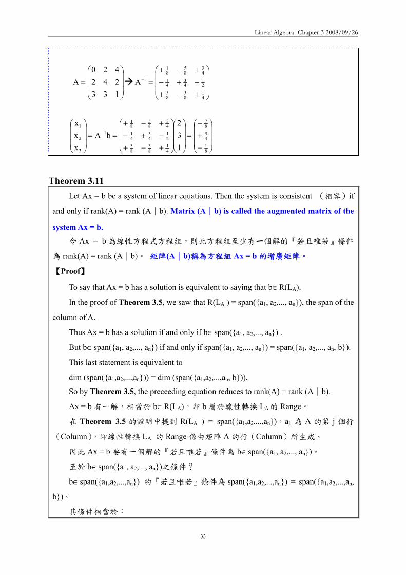
Linear Algebra- Chapter 3 20080926
33
⎟⎟⎟
⎠
⎞
⎜⎜⎜
⎝
⎛=
133242420
A⎟⎟⎟
⎠
⎞
⎜⎜⎜
⎝
⎛
+minus+minus+minus+minus+
=minus
41
83
83
21
43
41
43
85
81
1A
⎟⎟⎟
⎠
⎞
⎜⎜⎜
⎝
⎛
minus+minus
=⎟⎟⎟
⎠
⎞
⎜⎜⎜
⎝
⎛
⎟⎟⎟
⎠
⎞
⎜⎜⎜
⎝
⎛
+minus+minus+minus+minus+
==⎟⎟⎟
⎠
⎞
⎜⎜⎜
⎝
⎛minus
814587
41
83
83
21
43
41
43
85
81
1
3
2
1
132
bAxxx
Theorem 311 Let Ax = b be a system of linear equations Then the system is consistent (相容)if
and only if rank(A) = rank (A∣b) Matrix (A b) is called the augmented matrix o∣ f the
system Ax = b
令 Ax = b 為線性方程式方程組則此方程組至少有一個解的『若且唯若』條件
為 rank(A) = rank (A∣b) 矩陣(A∣b)稱為方程組 Ax = b 的增廣矩陣
【Proof】
To say that Ax = b has a solution is equivalent to saying that bisinR(LA)
In the proof of Theorem 35 we saw that R(LA ) = span(a1 a2 an) the span of the
column of A
Thus Ax = b has a solution if and only if bisinspan(a1 a2 an)
But bisinspan(a1 a2 an) if and only if span(a1 a2 an) = span(a1 a2 an b)
This last statement is equivalent to
dim (span(a1a2an)) = dim (span(a1a2an b))
So by Theorem 35 the preceeding equation reduces to rank(A) = rank (A∣b)
Ax = b 有一解相當於 bisinR(LA)即 b 屬於線性轉換 LA的 Range
在 Theorem 35 的證明中提到 R(LA ) = span(a1a2an)aj 為 A 的第 j 個行
(Column)即線性轉換 LA 的 Range 係由矩陣 A 的行(Column)所生成
因此 Ax = b 要有一個解的『若且唯若』條件為 bisinspan(a1 a2 an)
至於 bisinspan(a1 a2 an)之條件
bisinspan(a1a2an) 的『若且唯若』條件為 span(a1a2an) = span(a1a2an
b)
其條件相當於
Linear Algebra- Chapter 3 20080926
34
dim (span(a1a2an)) = dim (span(a1a2an b))
依據 Theorem 35該條件可簡化為 rank(A) = rank (A∣b)
Theorem 35 The rank of any matrix equals the maximum number of its linearly
independent columns that is the rank of a matrix is the dimension of the subspace
generated by its column任一矩陣的 Rank 等於其最大線性獨立行向量數目即矩陣的
Rank 是由矩陣的行向量生成的子空間的維度【LA Fn Fm】
EXAMPLE 5 Recall the system of equations
1xx0xx
21
21
=+=+
Since ⎟⎟⎠
⎞⎜⎜⎝
⎛=
1111
A and ⎟⎟⎠
⎞⎜⎜⎝
⎛=
111011
)bA(
rank(A) = 1 and rank (A b) = 2∣
Because the two ranks are unequal the system has no solutions
矩陣 A 與增廣矩陣(A∣b) 的 Rank 不同故方程組沒有解
EXAMPLE 6 We can use Theorem 311 to determine whether (3 3 2) is in the range of the linear
transformation T R3 R3 defined by T(a1 a2 a3) = (a1+a2+a3 a1-a2+a3 a1+a3)
利用 Theorem 311 來判斷 (3 3 2)是否在線性轉換 T 的 Range 中其中T R3
R3 定義為 T(a1 a2 a3) = (a1+a2+a3 a1-a2+a3 a1+a3)
Now (3 3 2)isinR(T) if and only if there exists a vector s = x1 x2 x3 in R3 such that
T(s)=(3 3 2) Such a vector s must be a solution to the system
2xx3xxx3xxx
31
321
321
=+=+minus=++
Since the ranks of the coefficient matrix and the augmented matrix of this system
are 2 and 3 respectively it follows that this system has no solutions Hence (3 3 2) notin
R(T)
(3 3 2)isinR(T) 的『若且唯若』的條件為存在一向量 s = x1 x2 x3isinR3 使得
T(s)=(3 3 2)
Linear Algebra- Chapter 3 20080926
35
向量 s 必須是 2xx3xxx3xxx
31
321
321
=+=+minus=++
的解
因係數矩陣⎟⎟⎟
⎠
⎞
⎜⎜⎜
⎝
⎛minus
101111111
的 Rank 為 2增廣矩陣⎟⎟⎟
⎠
⎞
⎜⎜⎜
⎝
⎛minus
233
101111111
的 Rank 為 3兩
者不相等故方程組無解(3 3 2) notin R(T)
Theorem 311 Let Ax = b be a system of linear equations Then the system is consistent
(相容)if and only if rank(A) = rank (A∣b) Matrix (A b) is called the ∣ augmented
matrix of the system Ax = b 令 Ax = b 為線性方程式方程組則此方程組至少有一個
解的『若且唯若』條件為 rank(A) = rank (A∣b) 矩陣(A∣b)稱為方程組 Ax = b 的
增廣矩陣
Application
In 1973 Wassily Leontief won the Nobel prize in economics for his work in developing
a mathematical model that can be used to describe various economic phenomena
1973 年Wassily Leontief 因研究一數學模式來描述各種經濟現象而獲頒諾貝爾經
濟獎
CLOSED MODEL
We begin by considering a simple society composed of three peoples (industries) ndash a
farmer who gows all the food a tailor who makes all the clothing and a carpenter who builds
all the housing We assume that each person sells to and buy from a central pool and that
everything produced is consumed Since no commodities either enter or leave the system this
case is referred to as the CLOSE MODEL
考慮一個單純社會的三種人生產食物的農夫製衣的裁縫師與蓋住屋的木匠
並假設採取集中聯營買賣且每一件產品皆付諸消費由於過程中沒有任何成品進入
或脫離這個系統所以稱為「封閉模式」
Each of these three individual consumes all three of the commodities produced in the
Linear Algebra- Chapter 3 20080926
36
society Suppose that the proportion of each of the commodities consumed by each person is
given in the following table
社會中每一位皆消費所生產的三種成品且每一種產品也都被三位所消費其消
費比例如下
食物 Food 衣物 Clothing 住屋 Housing
農夫 Farmer 040 020 020
裁縫師 Tailor 010 070 020
木匠 Carpenter 050 010 060
Let p1 p2 and p3 denote the incomes of the farmer tailor and carpenter respectively To
ensure that this society survives we require that the consumption of each individual equals
his or her income
令 p1p2 與 p3 分別表示農夫裁縫師與木匠的收入並為確保這個封閉社會可以
存活假設每一位的收入等於消費
Note that the farmer consumes 20 of the clothing Because the total cost of all clothing
is p2 the tailorrsquos income the amount spent by the farmer on clothing is 020 p2 Moreover the
amount spent by the farmer on food clothing and housing must equal the farmerrsquos income
and so we obtain the equation 040 p1 + 020 p2 + 030 p3 = p1
對農夫而言農夫的衣物消費佔 20然因所有衣物的消費總額 p2 等於裁縫師的
收入所以農夫在衣物上的消費為 020 p2且農夫在食物衣物與住屋的總消費要等
於農夫的收入 p1所以農夫的收入與消費關係式
040 p1 + 020 p2 + 020 p3 = p1
Similary equations describing the expenditures of the tailor and carpenter produce the
following system of linear equations
同理分別對裁縫師與木匠進行討論可獲得下列方程組
Linear Algebra- Chapter 3 20080926
37
040 p1 + 020 p2 + 020 p3 = p1
010 p1 + 070 p2 + 020 p3 = p2
050 p1 + 010 p2 + 060 p3 = p3
This system can be written as Ap = p
其中⎟⎟⎟
⎠
⎞
⎜⎜⎜
⎝
⎛=
3
2
1
ppp
p 且⎟⎟⎟
⎠
⎞
⎜⎜⎜
⎝
⎛=
600100500200700100200200400
A 稱為輸入-輸出(或消費)矩陣
(Input-output (or consumption) matrix)
Ap = p 稱為均衡條件(Equilibrium condition)
能否利用不等式 p ≦ p 來替代等式
At first it may seem reasonable to replace the equilibrium condition by the inequality
Ap ≦ p that is the requirement that consumption not exceed production But in fact Ap ≦ p implies that Ap = p in the closed model
For otherwise there exists a k for which
sumgt
jjkjk pAp
Hence since the columns of A sum to 1
sumsumsumsum ==gt
jj
i jjij
ii ppAp which is a contradiction (出現矛盾)
答案是在封閉系統中Ap ≦ p Ap = p
One solution to the homogeneous system (I ndash A) x = 0 which is equivalent to the
equilibrium condition is ⎟⎟⎟
⎠
⎞
⎜⎜⎜
⎝
⎛=
400350250
p
Linear Algebra- Chapter 3 20080926
38
齊次方程組(I ndash A) x = 0 或均衡條件的一個解為 ⎟⎟⎟
⎠
⎞
⎜⎜⎜
⎝
⎛=
400350250
p
We may interpret this to mean that the society survives if the farmer taior and carpenter
have incomes in the proportions 253540
⎟⎟⎟
⎠
⎞
⎜⎜⎜
⎝
⎛=
400350250
p 可以解釋為若農夫裁縫師與木匠收入比例為 253540則社會將
能生存下去
Theorem 312
Let A be an ntimesn input-output matrix having the form ⎟⎟⎠
⎞⎜⎜⎝
⎛=
EDCB
A where D is a 1times(n-
1) positive vector and C is an (n-1)times1 positive vector Then (I-A)x = 0 has a one-
dimensional solution set that is generated by a nonnegative vector
設 A 為 ntimesn 輸入-輸出矩陣 ⎟⎟⎠
⎞⎜⎜⎝
⎛=
EDCB
A 其中D 為 1times(n-1)正向量C 為
(n-1)times1 正向量則(I-A)x = 0 具有一維解集合且該解集合係由一非負向量所生成
Any input-output matrix with all positive entries satisfies the hypothesis of this theorem
任何輸入-輸出矩陣滿足 Theorem 312 的基本假設條件例如
⎟⎟⎟
⎠
⎞
⎜⎜⎜
⎝
⎛=
02502503502500650500750
A
OPEN MODEL
In the OPEN MODEL we assume that there is an outside demand for each of the
commodities produced Returning to our simple society let x1 x2 and x3 be the monetary
values of food clothing and housing produced with respective outside demands d1 d2 and d3
Let A be the 3times3 matrix such that Aij represents the amount of commodity i required to
Linear Algebra- Chapter 3 20080926
39
produce one monetary unit of commodity j Then the value of the surplus of food in the
society is x1 ndash (A11x1+A12x2+A13x3) that is the value of food produced minus the value of
food consumed while producing the three commodities The assumption that everything
produced is consumed gives us a similar equilibrium condition for the open model namely
that the surplus of each of the three commodities must equal the corresponding outside
demands Hence i
3
1jjiji dxAx =minussum
=
for j=1 2 3
在「開放模式」中我們假設每一產品皆有外來的需求在前述的單純社會裡
令 x1x2 與 x3 分別代表食物衣物與住屋的貨幣價值d1d2 與 d3 為食物衣物與住
屋的外來需求價值令 A 為 3times3 矩陣Aij 表示生產『一個貨幣單位』的產品 j 所需要
的產品 i 的價值於是此社會中食物的盈餘價值為 x1 ndash (A11x1+A12x2+A13x3)即食物的
價值減去生產食物衣物與住屋所需消耗的食物的價值意即生產出來的食物價值扣
掉用去生產食物衣物與住屋所消耗掉的價值)(A11A12A13 為生產一個貨幣單位
的食物 1衣物 2 與住屋 3 所需消耗的食物 1 數量A12x2 表示生產貨幣價值為 x2的衣物
所需要的食物價值)對每一種產品而言其盈餘價值等於外來的需求價值於是
i
3
1jjiji dxAx =minussum
=
for j=123
Suppose that 30 cents worth of food 10 cents worth of clothing and 30 cents worth of
housing are required for the production of $1 worth of food Similar suppose that 20 cents
worth of food 40 cents worth of clothing and 20 cents worth of housing are required for the
production of $1 worth of clothing Finally suppose that 30 cents worth of food 10 cents
worth of clothing and 30 cents worth of housing are required for the production of $1 worth
of housing Then the input-output matrix is
⎟⎟⎟
⎠
⎞
⎜⎜⎜
⎝
⎛=
300200300100400100300200300
A
假設生產價值 1 元的食物需要價值 30 分的食物(A11 = 03)價值 10 分的衣物
(A21 = 01)及價值 30 分的住屋(A31 = 03)生產價值 1 元的衣物需要價值 20 分的
食物(A12 = 02)價值 40 分的衣物(A22 = 04)及價值 20 分的住屋(A32 = 02)生
Linear Algebra- Chapter 3 20080926
40
產價值 1 元的住屋需要價值 30 分的食物(A13 = 03)價值 10 分的衣物(A23 = 01)
及價值 30 分的住屋(A33 = 03)於是輸入輸出矩陣 A 為
⎟⎟⎟
⎠
⎞
⎜⎜⎜
⎝
⎛=
300200300100400100300200300
A
若食物的外來需求值為 300 億元衣物為 200 億元住屋值為 1 百億元則
⎟⎟⎟
⎠
⎞
⎜⎜⎜
⎝
⎛=
⎟⎟⎟
⎠
⎞
⎜⎜⎜
⎝
⎛
⎟⎟⎟
⎠
⎞
⎜⎜⎜
⎝
⎛
minusminusminusminusminusminus
=minus=
minus
minus
700600900
100200300
700200300100600100300200300
d)AI(x
1
1
⎟⎟⎟
⎠
⎞
⎜⎜⎜
⎝
⎛=
700600900
x 表示要滿足外來需求必須生產的食物價值為 900 億元衣物價值為
600 億元住屋價值為 700 億元
Theorem
Let AX = Y be a system of n linear equations in n variables If Andash1 exists the
solution is unique and is given by X = Andash1Y
【Proof】
Substitute X = Andash1Y into the matrix equation
AX = A(Andash1Y) = (AAndash1)Y = InY = Y
The solution is unique
Let X1 be any solution thus AX1 = Y Multiplying both sides of this equation by Andash1
gives
Andash1AX1= Andash1Y InX1 = Andash1Y X1 = Andash1Y
Linear Algebra- Chapter 3 20080926
41
Example Example 1212
2x5x3x3x5x3x21x2x x
321
321
321
minus=++minus=minusminus=minusminus
⎥⎥⎥
⎦
⎤
⎢⎢⎢
⎣
⎡
minus=
⎥⎥⎥
⎦
⎤
⎢⎢⎢
⎣
⎡
⎥⎥⎥
⎦
⎤
⎢⎢⎢
⎣
⎡
minusminusminusminusminus
231
xxx
531532211
3
2
1
Solve the system of equations
This system can be written in the following matrix form
⎥⎥⎥
⎦
⎤
⎢⎢⎢
⎣
⎡
minus⎥⎥⎥
⎦
⎤
⎢⎢⎢
⎣
⎡
minusminusminusminusminus
=
⎥⎥⎥
⎦
⎤
⎢⎢⎢
⎣
⎡minus
231
531532211
xxx 1
3
2
1
If the matrix of coefficients is invertible the unique solutionIf the matrix of coefficients is invertible the unique solution isis
Example Example 2222
1 2 1 issolution unique The 321 =minus== xxx
⎥⎥⎥
⎦
⎤
⎢⎢⎢
⎣
⎡minus=
⎥⎥⎥
⎦
⎤
⎢⎢⎢
⎣
⎡
minus⎥⎥⎥
⎦
⎤
⎢⎢⎢
⎣
⎡
minusminusminus=
⎥⎥⎥
⎦
⎤
⎢⎢⎢
⎣
⎡
121
231
123135110
xxx
3
2
1
⎥⎥⎥
⎦
⎤
⎢⎢⎢
⎣
⎡
minusminusminus=
⎥⎥⎥
⎦
⎤
⎢⎢⎢
⎣
⎡
minusminusminusminusminus
=
minus
minus
123135110
531532211
A
1
1
The The LeontiefLeontief IO Model in IO Model in Economics Economics 1515
The Leontief input-output model is used to analyze the interdependence of economics Wassily Leontief received a Nobel Prize in 1973 for his work in thie fieldThe practical applications of this model have proliferated until it has now become a standard tool for investigating economic structures ranging from cities and corporation to states and countriesConsider an economics situation that involves ninterdependent industries The output of any one industry is needed as input by other industries and even possibly by the industry itself
The The LeontiefLeontief IO Model in IO Model in Economics Economics 2525
How a mathematical model involving a system of linear equations can be constructed to analyze such a situationAssume that each industry produces one commodity Let aij denote the amount of input of a certain commodity i to produce unit output of commodity j In our model let the amounts of input and output be measured in dollars Thus for example a34 = 045 means that 45 centsrsquo worth of commodity 3 is required to produce one dollarrsquos worth of commodity 4
The The LeontiefLeontief IO Model in IO Model in Economics Economics 3535
aij = amount of commodity i in one dollar of commodity jaij =生產一元價值的j產品需要耗用的i產品價值
The elements aij called input coefficients define a matrix A called the input-output matrix which describes the interdependence of the industriesExtending the model to include an open sector (all non-producing sectors) The product of industries may go not only into other producing industries but also into other non-producing sectors of the economy such as consumers and governments
The The LeontiefLeontief IO Model in IO Model in Economics Economics 4545
di = demand of the open sectors from industry ixi=total output of industry I necessary to meet demands of all n industries and the open sector
sectoropen of demand
nindustry of demand
2industry of demand
22
1industry of demand
11
industry ofoutput total
ininii
i
i dxaxaxax ++sdotsdotsdot++=
output ofportion sectoropen
output ofportion tryinterindusoutput total
DAXX +=Demand matrixDemand matrix
Output matrixOutput matrix
The The LeontiefLeontief IO Model in IO Model in Economics Economics 5555
Applying the model to the economy of a country X Applying the model to the economy of a country X represents the total output of each of the producing sectors represents the total output of each of the producing sectors of the economy and AX describes the contributions made of the economy and AX describes the contributions made by the various sectors to fulfilling the intersectional input by the various sectors to fulfilling the intersectional input requirements of the economyrequirements of the economyD is equal to (XD is equal to (X--AX) the difference between total output AX) the difference between total output X and industry transaction AXX and industry transaction AXD is thus the gross national product of the economyD is thus the gross national product of the economy
Example Example 1414
Consider an economy consisting of three industries having Consider an economy consisting of three industries having the following inputthe following input--output matrix output matrix AA Determine the output Determine the output levels required of the industries to meet the demands of levels required of the industries to meet the demands of the other industries and of the open sector in each casethe other industries and of the open sector in each case
in turn 321812
and 896
1612
9
5100
021
21
103
51
51
⎥⎥⎦
⎤
⎢⎢⎣
⎡
⎥⎥⎦
⎤
⎢⎢⎣
⎡
⎥⎥⎦
⎤
⎢⎢⎣
⎡=
⎥⎥⎥
⎦
⎤
⎢⎢⎢
⎣
⎡
= DA
The unit of The unit of DD are millions of dollarsare millions of dollars
Linear Algebra- Chapter 3 20080926
42
Example Example 2424
We wish to compute the output levels X that correspond to We wish to compute the output levels X that correspond to the various open sector demands D X is given by the the various open sector demands D X is given by the equation X = AX + D Rewritten as followsequation X = AX + D Rewritten as follows
X ndash AX = D rArr (I ndash A)X = D rArr X = (I ndash A) ndash1 D
⎥⎥⎥
⎦
⎤
⎢⎢⎢
⎣
⎡
=⎥⎥⎥
⎦
⎤
⎢⎢⎢
⎣
⎡
minus⎥⎥⎦
⎤
⎢⎢⎣
⎡=minus minus
minusminus
5400
021
21
103
51
54
5100
021
21
103
51
31
100010001
get We AI
⎥⎥⎥
⎦
⎤
⎢⎢⎢
⎣
⎡
=minus minus
4500
038
35
85
32
35
1)( AI
output ofingcorrespond valuesvarious
4500
038
35
85
32
35
)(
401020883957522133
32816189121269
)(
1
1
DAI
DAIX
minus
minus
minusuarruarruarruarruarruarruarr
⎥⎥⎦
⎤
⎢⎢⎣
⎡=
⎥⎥⎦
⎤
⎢⎢⎣
⎡
⎥⎥⎥
⎦
⎤
⎢⎢⎢
⎣
⎡
=minus=
Example Example 3434
By using Gauss-Jordan elimination
dollars of milliond are units The
40
15674
and 106629
209946
are 321812
and 896
1612
9
⎥⎥⎥
⎦
⎤
⎢⎢⎢
⎣
⎡
⎥⎥⎥
⎦
⎤
⎢⎢⎢
⎣
⎡
⎥⎥⎥
⎦
⎤
⎢⎢⎢
⎣
⎡
⎥⎥⎥
⎦
⎤
⎢⎢⎢
⎣
⎡
⎥⎥⎥
⎦
⎤
⎢⎢⎢
⎣
⎡
⎥⎥⎥
⎦
⎤
⎢⎢⎢
⎣
⎡
Example Example 4444
The output levels necessary to meet the demandsThe output levels necessary to meet the demands
IAAAIAI m =++++minus ))(( 2 L
mAAAIAI ++++=minus minus L21)(
Computing (IComputing (I--A) A) --11
1m
m2m2
m2
AI)AAAI(A)AAAI(I
)AAAI)(AI(
+minus=++++minus++++=
++++minusLL
L
NOTE 0A 1m rarr+
Population Movement Population Movement 1313
In 2000 58 million of people live in cities and 142 million of In 2000 58 million of people live in cities and 142 million of people people live in the surrounding suburbs Represent this information by tlive in the surrounding suburbs Represent this information by the he matrix matrix
The probability of a person staying in the city was 096 Thus tThe probability of a person staying in the city was 096 Thus the he probability of moving to the suburbs was 004 probability of moving to the suburbs was 004 The probability of a person moving to the city was 001 the The probability of a person moving to the city was 001 the probability of remaining in suburbia was 099probability of remaining in suburbia was 099
suburbcity
990040010960
suburbcity (to))from(
⎥⎦
⎤⎢⎣
⎡=P
⎥⎦
⎤⎢⎣
⎡=
14258
X0
City population in 2001 = people who remained from 2000 + peopleCity population in 2001 = people who remained from 2000 + peoplewho moved in from the suburbs = ( 096 who moved in from the suburbs = ( 096 timestimes 58 ) + (001 58 ) + (001 timestimes 142 ) = 142 ) = 571 million571 millionSuburban population in 2001 = people who moved in from the city Suburban population in 2001 = people who moved in from the city + people who stayed from 2000 = ( 004 + people who stayed from 2000 = ( 004 timestimes 58 ) + (099 58 ) + (099 timestimes 142 ) = 142 ) = 1429 million1429 millionCan arrive at these numbers using matrix multiplicationCan arrive at these numbers using matrix multiplication
⎥⎦
⎤⎢⎣
⎡=⎥
⎦
⎤⎢⎣
⎡⎥⎦
⎤⎢⎣
⎡==
9142157
14258
990040010960
PXX 01
Population Movement Population Movement 2323
Population Movement Population Movement 3333
Assume that the population flow represented by the matrix P is unchanged over the years The population distribution X2 after 2 years is given by X2 = P X1 = P2 X0 In general
Pn is called the n-step transition matrix The (ij)th element of Pngives the probability of going from state j to state i in n stepsFor example
in
ni XPX =+
suburbcity
960150040850
P
suburbcity (to))from(
4
⎥⎦
⎤⎢⎣
⎡=
The probability of living in the city in The probability of living in the city in 2000 and being in the suburbs 4 years 2000 and being in the suburbs 4 years later is 015later is 015
Markov ChainsMarkov Chains
The probabilities in the above model depend only on the The probabilities in the above model depend only on the current state of a person whether the person is living in the current state of a person whether the person is living in the city or in suburbiacity or in suburbiaThis type of model in which the probability of going from This type of model in which the probability of going from one state to another depends only on the current state one state to another depends only on the current state rather than on a more complete historical description is rather than on a more complete historical description is called a called a Markov chainMarkov chainMarkov chains are useful tools for scientists in many Markov chains are useful tools for scientists in many fields such as geneticsfields such as genetics
Linear Algebra- Chapter 3 20080926
43
GeneticsGenetics 1414
Genetics is the branch of biology that deals with Genetics is the branch of biology that deals with heredity heredity (遺傳)(遺傳) It is the study of units called It is the study of units called genes which determine the characteristics living genes which determine the characteristics living things inherit from their parents The inheritance things inherit from their parents The inheritance (遺傳)(遺傳)of such traitsof such traits(特徵)(特徵)as sex height eye as sex height eye color and hair color of human beings and such color and hair color of human beings and such traits as petaltraits as petal(花瓣)(花瓣) color and leaf shape of color and leaf shape of plants are governed by genesplants are governed by genesIn medicine agricultureIn medicine agriculturehelliphellip
GeneticsGenetics 2424
The traits of guinea pigsThe traits of guinea pigs(天竺鼠)(天竺鼠)are long hair and short hairare long hair and short hairThe length of hair is governed by a pair of gene which we denoteThe length of hair is governed by a pair of gene which we denote A A and aand aA guinea pig may have any one of the combination of AA A guinea pig may have any one of the combination of AA AaAa or or aaaa Each of these classes is called a genotypeEach of these classes is called a genotype(基因型)(基因型)The AA type guinea pig is indistinguishable in appearance from tThe AA type guinea pig is indistinguishable in appearance from the he AaAa type type ndashndash both have long hair both have long hair ndashndash whereas the whereas the aaaa type has short hairtype has short hairThe A gene is said to dominate the a geneThe A gene is said to dominate the a geneAn animal is called dominant An animal is called dominant (顯性)(顯性)if it has AA genes hybridif it has AA genes hybrid(混種)(混種) with with AaAa genes and recessive genes and recessive (隱性)(隱性)with with aaaa genesgenes
GeneticsGenetics 3434
When two guinea pigs are crossed the offspring inherits one genWhen two guinea pigs are crossed the offspring inherits one gene e from each parent in random mannerfrom each parent in random mannerGiven the genotype of the parents we can determine the Given the genotype of the parents we can determine the probabilities of the genotype of the offspringprobabilities of the genotype of the offspring
AA+AA AA+AA probabilities of AA probabilities of AA AaAa and and aaaa are 10and 0are 10and 0Aa+AAAa+AA probabilities of AA probabilities of AA AaAa and and aaaa are are frac12frac12 frac12frac12 and 0 and 0aa+AAaa+AA probabilities of AA probabilities of AA AaAa and and aaaa are 0 1 and 0are 0 1 and 0
This series of experiments is a Markov chain having transition This series of experiments is a Markov chain having transition matrixmatrix
aaAaAA
00012100211
P
aaAaAA
⎥⎥⎥
⎦
⎤
⎢⎢⎢
⎣
⎡=
GeneticsGenetics 4444
Assume an initial population of guinea pigs made up of an Assume an initial population of guinea pigs made up of an equal number of each genotypeequal number of each genotype
⎥⎥⎥
⎦
⎤
⎢⎢⎢
⎣
⎡=
313131
X0
The fractions of following generations are
⎥⎥⎥
⎦
⎤
⎢⎢⎢
⎣
⎡=
⎥⎥⎥
⎦
⎤
⎢⎢⎢
⎣
⎡=
⎥⎥⎥
⎦
⎤
⎢⎢⎢
⎣
⎡=
⎥⎥⎥
⎦
⎤
⎢⎢⎢
⎣
⎡=
01611615
X08187
X04143
X02121
X 4321
AAAAAaAaaaaa
3-4 Systems of Linear Equations ndash Computational Aspects
DEFINITION 36 Equivalent
Two systems of linear equations are called equivalent if they have the same solution
set
兩個線性方程組稱為等價意指兩者具有相同的解集合
Elementary Transformations Transformation called elementary transformations can be used to change a system of
linear equations into another system of linear equations that have the same solution
These transformations are used to solve system of linear equations by eliminating
variables
The equivalent transformations used in terms of matrix are called ELEMENTARY
ROW OPERATION
Linear Algebra- Chapter 3 20080926
44
Equivalent System Systems of equations that are related through elementary transformations are called
equivalent systems
Matrices that are related through elementary row operations are called row equivalent
matrices
The symbol asymp is used to indicate equivalence in both cases
Theorem 313 Let Ax = b be a system of m linear equations in n unknowns and let C be an invertible
mtimesm matrix Then the system (CA)x = Cb is equivalent to Ax = b
設 Ax = b 為含 n 個未知數m 個線性方程式的方程組若 C 為可逆的mtimesm
矩陣則(CA)x = Cb 等價於 Ax = b
【Proof】
Let K be the solution set for Ax = b and Krsquo the solution set for (CA)x = Cb If wisinK
then Aw = b So (CA)w = Cb and hence wisinKrsquo Thus KsubeKrsquo
Conversely if wisinKrsquo then (CA)w = Cb Hence Aw = C-1(CA)w = C-1(Cb) = b so
wisinK Thus KrsquosubeK and therefore K=Krsquo
設 K 為 Ax = b 的解集合且 Krsquo為(CA)x = Cb 的解集合
若 wisinK則 Aw = b (CA)w = Cb故 wisinKrsquo於是 KsubeKrsquo
反之若 wisinKrsquo則(CA)w = Cb Aw = C-1(CA)w = C-1(Cb) = b故 wisinK於是
KrsquosubeK因此K=Krsquo
Corollary Let Ax = b be a system of m linear equations in n unknowns If (Arsquo brsquo) is obtained ∣
from from (A b) by a finite number of elementary row operations then the system Arsquox = ∣
brsquo is equivalent to the original system
設 Ax = b 為含 n 個未知數m 個線性方程式的方程組若(Arsquo brsquo) ∣ 是由(A b) ∣
經過有限次數的基本列運算而得則 Arsquox = brsquo 等價於 Ax = b即兩者具有相同的解
集合
【Proof】
Suppose that (Arsquo brsquo) is obtained from (A b) by elementary row operations These ∣ ∣
Linear Algebra- Chapter 3 20080926
45
may be executed by multiplying (A b) by elementary mtimesm matrices E∣ 1 E2hellipEp Let
C=EphellipE2E1 then (Arsquo brsquo) = C(A b) = (CA Cb)∣ ∣ ∣
Since each Ei is invertible so is C Now Arsquo = CA and brsquo = Cb Thus by Theorem 313
the system Arsquox = brsquo is equivalent to the system Ax = b
設(Arsquo brsquo)∣ 是由(A b)∣ 經過基本列運算取得即以基本 mtimesm 矩陣 E1 E2hellipEp
乘上 (A b)∣ (Arsquo brsquo) = C(A b) = (CA Cb∣ ∣ ∣ )其中C=EphellipE2E1
因 Ei 可逆故 C 亦為可逆 Arsquo = CA 且 brsquo = Cb
依據 Theorem 313Arsquox = brsquo 等價於 Ax = b
Theorem 313 Let Ax = b be a system of m linear equations in n unknowns and let C be an
invertible mtimesm matrix Then the system (CA)x = Cb is equivalent to Ax = b 設 Ax = b
為含 n 個未知數m 個線性方程式的方程組若 C 為可逆的mtimesm 矩陣則(CA)x
= Cb 等價於 Ax = b
We now describe a method for solving any stystem of linear equations Consider for
example the system of linear equations
探討解線性方程組的方法hellip
2xxx2x3xxx1x2x3x2x3
4321
321
4321
=minus++=++=minus++
First we form the augmented matrix ⎟⎟⎟
⎠
⎞
⎜⎜⎜
⎝
⎛
minus
minus
231
112101112323
(增廣矩陣)
Interchanging the first and third rows ⎟⎟⎟
⎠
⎞
⎜⎜⎜
⎝
⎛
minus
minus
132
132301111121
(第 13 列互調)
Adding -1 times the first row to the second row and then add -3 times the first row to
the third row ⎟⎟⎟
⎠
⎞
⎜⎜⎜
⎝
⎛
minusminusminus
minus
512
104010101121
(第 1 列乘上 -1 加到第 2 列再以 -3 乘上
第 1 列加到第 3 列)
Linear Algebra- Chapter 3 20080926
46
Multiplying the second row by -1 ⎟⎟⎟
⎠
⎞
⎜⎜⎜
⎝
⎛
minusminus
minusminusminus
51
2
104010101121
(第 2 列乘上 -1)
Adding four times the second row to the third row ⎟⎟⎟
⎠
⎞
⎜⎜⎜
⎝
⎛
minusminus
minusminusminus
91
2
300010101121
(4 乘上第 2
列加到第 3 列)
Multiplying the third row by -13 ⎟⎟⎟
⎠
⎞
⎜⎜⎜
⎝
⎛minusminus
minus
31
2
100010101121
(第 3 列乘上 -13)
Adding the third row to the first and second rows to obtain zeros in row 1 column 4
and row 2 column 4 ⎟⎟⎟
⎠
⎞
⎜⎜⎜
⎝
⎛
325
100000100121
(將第 3 列加到第 1 列及第 2 列)
Adding -2 times the second row to the first row in order to make the first row second
column entry become zero ⎟⎟⎟
⎠
⎞
⎜⎜⎜
⎝
⎛
321
100000100101
(將第 2 列乘以 -2 再加至第 1 列)
We have now obtained the desired reduction of the augmented matrix
⎟⎟⎟
⎠
⎞
⎜⎜⎜
⎝
⎛
321
100000100101
是化簡後的增廣矩陣
This matrix corresponds to the system of linear equations
對應的線性方程組為
2x3x1xx
4
2
31
===+
By Corollary to Theorem 313 this system is equivalent to the original system But this
system is easily solved Obviously x2 = 2 and x4 = 3 Moreover x1 and x3 can be any values
Linear Algebra- Chapter 3 20080926
47
provided their sum is 1 Letting x3 = t we then have x1 = 1 ndash t Thus an arbitray solution to the
original system has the form
依據 Corollary to Theorem 313 化簡後的方程組與原方程組等值此方程組的解為
x2 = 3x4 = 3x1 + x3 = 1於是原方程組的任意解可以寫成
⎟⎟⎟⎟⎟
⎠
⎞
⎜⎜⎜⎜⎜
⎝
⎛minus
+
⎟⎟⎟⎟⎟
⎠
⎞
⎜⎜⎜⎜⎜
⎝
⎛
=
⎟⎟⎟⎟⎟
⎠
⎞
⎜⎜⎜⎜⎜
⎝
⎛ minus
0101
t
3021
3t2
t1
Observe that
⎪⎪⎭
⎪⎪⎬
⎫
⎪⎪⎩
⎪⎪⎨
⎧
⎟⎟⎟⎟⎟
⎠
⎞
⎜⎜⎜⎜⎜
⎝
⎛minus
0101
is a basis for the homogeneous system of equations
corresponding to the given system
其中
⎪⎪⎭
⎪⎪⎬
⎫
⎪⎪⎩
⎪⎪⎨
⎧
⎟⎟⎟⎟⎟
⎠
⎞
⎜⎜⎜⎜⎜
⎝
⎛minus
0101
是齊次方程組解集合的一組基底
Gauss-Jordan Elimination
Let A be an n times n matrix
1 Adjoin the identity n times n matrix In to A to form the matrix [A In]
2 Compute the reduced echelon form of [A In]
(1) If the reduced echelon form is of the type [In B] then B is the inverse of A
(2) If the reduced echelon form is not of the type [In B] in that the first n times n
submatrix is not In then A has no inverse
An n times n matrix A is invertible if and only if its reduced echelon form is In
DEFINITION 37 Reduced Row Echelon Form
A matrix is said to be in reduced row echelon form if the following three conditions
are satisfied
Linear Algebra- Chapter 3 20080926
48
一個矩陣可以被稱為簡約列梯形式必須具備有下列三條件
(a) Any row containing a nonzero entry preceeds any row in which all the entries are
zero (if any)
含有非零元素的任一列排在全含零元素的任一列前面(儘可能)
(b) The first nonzero entry in each row in the only nonzero entry in its column
各列中第一個非零元素為其所在行中唯一的非零元素
(c) The first nonzero entry in each row is 1 and it occurs in a column to thr right of the
first nonzero entry in the preceeding row
各列中第一個非零元素為 1 且它出現在前一列中第一個非零元素的右邊某一
行中
Reduced Echelon Form A matrix is in reduced echelon form if
1 Any rows consisting entirely of zeros are grouped at the bottom of the matrix
2 The first nonzero element of each other row is 1 This element is called a leading 1
3 The leading 1 of each row after the first is positioned to the right of the leading 1 of
the previous row
4 All other elements in a column that contains a leading 1 are zero
Theorem 314 Gaussian Elimination Transformation Gaussian elimination transform any matrix into its reduced row echelon form
利用 Gaussian elimination 將矩陣轉換成簡約列梯形式
We now describe a method for solving a system in which the augmented matrix is in
reduced row echelon form To illustrate this procedure we consider the system
14x8x3x2x2x28x5x2xxx6x3xxxx17x9x4xx3x2
54321
54321
54321
54321
=minus+++=minus+++=minus+++=minus+++
Linear Algebra- Chapter 3 20080926
49
for which the augmented matrix is
⎟⎟⎟⎟⎟
⎠
⎞
⎜⎜⎜⎜⎜
⎝
⎛
minusminusminusminus
1486
17
83222521113111194132
(增廣矩陣)
Applying Gaussian elimination to the augmented matrix of the system produces the
following sequence of matrices
利用 Gaussian elimination method 處理增廣矩陣
⎟⎟⎟⎟⎟
⎠
⎞
⎜⎜⎜⎜⎜
⎝
⎛
minusminusminusminus
1486
17
83222521113111194132
⎟⎟⎟⎟⎟
⎠
⎞
⎜⎜⎜⎜⎜
⎝
⎛
minusminusminusminus
148
176
83222521119413231111
⎟⎟⎟⎟⎟
⎠
⎞
⎜⎜⎜⎜⎜
⎝
⎛
minusminus
minus
0213
0000021000
1011020201
The system of linear equations corresponding to thus last matrix is
對應最後矩陣的線性方程組 2x2x
1xxx3x2x2x
54
532
531
=minus=+minus=minus+
Assign x3 = t1 x5 = t2
2t22x2x1tt1xxx
3t2t23x2x2x
254
21532
21531
+=+=+minus=+minus=
++minus=++minus=
Thus an arbitray solution s is of the form
於是任意解 s 具有下列形式
s =
⎟⎟⎟⎟⎟⎟
⎠
⎞
⎜⎜⎜⎜⎜⎜
⎝
⎛minus
+
⎟⎟⎟⎟⎟⎟
⎠
⎞
⎜⎜⎜⎜⎜⎜
⎝
⎛minus
+
⎟⎟⎟⎟⎟⎟
⎠
⎞
⎜⎜⎜⎜⎜⎜
⎝
⎛
=
⎟⎟⎟⎟⎟⎟
⎠
⎞
⎜⎜⎜⎜⎜⎜
⎝
⎛
+
+minus++minus
=
⎟⎟⎟⎟⎟⎟
⎠
⎞
⎜⎜⎜⎜⎜⎜
⎝
⎛
1201
2
t
00112
t
02013
t2t2
t1tt
3t2t2
xxxxx
21
2
2
1
21
21
5
4
3
2
1
where t1t2isinR
Linear Algebra- Chapter 3 20080926
50
Notice that
⎪⎪⎪
⎭
⎪⎪⎪
⎬
⎫
⎪⎪⎪
⎩
⎪⎪⎪
⎨
⎧
⎟⎟⎟⎟⎟⎟
⎠
⎞
⎜⎜⎜⎜⎜⎜
⎝
⎛minus
⎟⎟⎟⎟⎟⎟
⎠
⎞
⎜⎜⎜⎜⎜⎜
⎝
⎛minus
1201
2
00112
is a basis for the solution set of the corresponding
homogeneous system of equation and
⎟⎟⎟⎟⎟⎟
⎠
⎞
⎜⎜⎜⎜⎜⎜
⎝
⎛
02013
is a particular solution to the original system
⎪⎪⎪
⎭
⎪⎪⎪
⎬
⎫
⎪⎪⎪
⎩
⎪⎪⎪
⎨
⎧
⎟⎟⎟⎟⎟⎟
⎠
⎞
⎜⎜⎜⎜⎜⎜
⎝
⎛minus
⎟⎟⎟⎟⎟⎟
⎠
⎞
⎜⎜⎜⎜⎜⎜
⎝
⎛minus
1201
2
00112
是齊次方程組解集合的一組基底
⎟⎟⎟⎟⎟⎟
⎠
⎞
⎜⎜⎜⎜⎜⎜
⎝
⎛
02013
是原方程組的特別解
EXAMPLE 1
The matrix ⎟⎟⎟
⎠
⎞
⎜⎜⎜
⎝
⎛
101010011
is not in reduced row echelon form
因為第一行含有第一個非零元素在第一列但第一行尚含有其他非零元素
The matrix ⎟⎟⎟
⎠
⎞
⎜⎜⎜
⎝
⎛
110010012010
is not in reduced row echelon form
因為第一列第一個非零元素不在第一列第一個非零元素的右邊
The matrix ⎟⎟⎠
⎞⎜⎜⎝
⎛010002
is not in reduced row echelon form
因為第一列的第一個非零元素不是 1
Linear Algebra- Chapter 3 20080926
51
Reduced Echelon FormReduced Echelon Form
⎥⎥⎥
⎦
⎤
⎢⎢⎢
⎣
⎡
910030107001
⎥⎥⎥
⎦
⎤
⎢⎢⎢
⎣
⎡
100001000041
⎥⎥⎥
⎦
⎤
⎢⎢⎢
⎣
⎡
000210801
Not in Reduced Echelon Form
⎥⎥⎥
⎦
⎤
⎢⎢⎢
⎣
⎡
310000004021
⎥⎥⎥
⎦
⎤
⎢⎢⎢
⎣
⎡
100000430003021
⎥⎥⎥⎥
⎦
⎤
⎢⎢⎢⎢
⎣
⎡
0000210030108071
In Reduced Echelon Form
Use GaussUse Gauss--Jordan elimination to Jordan elimination to find reduced echelon formfind reduced echelon form 1313
Step 1 Interchange rows if necessary to bring a nonzero Step 1 Interchange rows if necessary to bring a nonzero element to the top of the first nonzero column This nonzero element to the top of the first nonzero column This nonzero element is called a pivotelement is called a pivot
⎥⎥⎦
⎤
⎢⎢⎣
⎡
minusminus
minus
1211244129333
22200
⎥⎥⎥
⎦
⎤
⎢⎢⎢
⎣
⎡
minusminus
minus
harrasymp
121124422200
129333
R2R1
Use GaussUse Gauss--Jordan elimination to Jordan elimination to find reduced echelon formfind reduced echelon form 2323
Step 2 Create a 1 in the pivot location by multiplying the Step 2 Create a 1 in the pivot location by multiplying the pivot row by 1pivotpivot row by 1pivot
Step 3 Create zero elsewhere in the pivot column by adding Step 3 Create zero elsewhere in the pivot column by adding suitable multiples of the pivot row to all other rows of the suitable multiples of the pivot row to all other rows of the matrixmatrix
⎥⎥⎥
⎦
⎤
⎢⎢⎢
⎣
⎡
minusminusminus
minus
minus+asymp
412002220043111
4)R1(R3
⎥⎥⎦
⎤
⎢⎢⎣
⎡
minusminus
minus
⎟⎠⎞
⎜⎝⎛asymp
12112442220043111
R13
1
The matrix is the reduced echelon form of the given matrixThe matrix is the reduced echelon form of the given matrix
Use GaussUse Gauss--Jordan elimination to Jordan elimination to find reduced echelon formfind reduced echelon form 3333
Step 4 Cover the pivot row and all rows above it Repeat Steps Step 4 Cover the pivot row and all rows above it Repeat Steps 1 1 and 2 for the remaining and 2 for the remaining submatrixsubmatrix Repeat Step 3 for the whole Repeat Step 3 for the whole matrix Continue until the reduced echelon form is reachedmatrix Continue until the reduced echelon form is reached
⎥⎥⎥
⎦
⎤
⎢⎢⎢
⎣
⎡
minusminus
+minus+asymp
⎥⎥⎥
⎦
⎤
⎢⎢⎢
⎣
⎡
minusminus
minus++asymp
⎥⎥⎥
⎦
⎤
⎢⎢⎢
⎣
⎡
minusminusminus
minus
⎟⎠⎞
⎜⎝⎛
asymp
⎥⎥⎥
⎦
⎤
⎢⎢⎢
⎣
⎡
minusminusminus
minus
6100050100
170011
R3R22)R3(R1
610001110052011
R2)2(R3R2R1
412001110043111
R221
412002220043111
Theorem 315 Let Ax = b be a system of r nonzero equations is in n unknown Suppose that rank(A)
= rank (A b)∣ and that (A b)∣ is in reduced row echelon form Then
設 Ax = b 為含有 n 個未知數r 個非零方程式的方程組假設 rank(A) = rank
(A b)∣ 且 (A b)∣ 為簡約列梯形式於是
(a) rank(A) = r
(b) If the general solution obtained by the procedure above is of the form s = s0 + t1u1
+ t2u2 +hellip+ tn-run-r then u1 u2hellip un-r is a basis for the solution set of the
corresponding homogeneous system and s0 is a solution to the original system 由
前述方法所得的 General solution 具有下列形式
s = s0 + t1u1 + t2u2 +hellip+ tn-run-r
其中u1 u2hellip un-r為齊次方程組 Ax = 0 的解集合的一組基底且 s0 為原方
程組的一個解)
【Proof】
Since (A b)∣ is in reduced row echelon form (A b)∣ must have r nonzero rows
Clearly these rows are linearly independent by the definition of the reduced row echelon
Linear Algebra- Chapter 3 20080926
52
form and so rank (A b)∣ = r Thus rank(A) = r
Let K be the solution set for Ax = b and let KH be the solution set for Ax = 0 Setting
t1 = t2 =hellip= tn-r = 0 we see that s = s0isinK But by Theorem 39 K = s +KH Hence
KH = - s0+K = span(u1 u2hellip un-r )
Because rank(A) = r we have dim(KH) = n-r Thus since dim(KH) = n-r and KH is
generated by a set u1 u2hellip un-r containing at most n-r vectors that is a basis for KH
由於(A b)∣ 具有簡約列梯形式因此(A b)∣ 必定具有 r 個非零列由簡約列梯形
式的定義得知 r 個非零列為線性獨立故 rank (A b)∣ = rrank(A) = r
令 K 為 Ax = b 的解集合 KH 為 Ax = 0 的解集合
假設 t1 = t2 =hellip= tn-r = 0(u1 u2hellip un-r非 KH的基底)則 s = s0isinK
依據 Theorem 39K = s +KH KH = - s0+K = span(u1 u2hellip un-r )
因 rank(A) = r所以 dim(KH) = n - r 且 KH 是由u1 u2hellip un-r 所生成
故原假設「t1 = t2 =hellip= tn-r = 0」不成立
因此 KH含有最多 n - r 個向量且這些向量為 KH的基底
Theorem 39 Let K be the solution set of a system of linear equations Ax = b and let KH be
the solution set of the corresponding homogeneous system Ax = 0 Then for any solution s
to Ax = b K =s + KH = s+k kisinKH 設 K 為線性方程組 Ax = b 的解集合且 KH
為對應的齊次方程組的解集合則對 Ax = b 的任一個解 s 而言K =s + KH = s+k
kisinKH
ExampleExampleSolve the system of equationsSolve the system of equations
7537429333
321
321
321
=minusminus=+minus=+minus
xxxxxxxxx
⎥⎥⎦
⎤
⎢⎢⎣
⎡
++asymp
000012104301
R2R3R2R1 12
431243
32
31
32
31+minus=+minus=rArr=+
=+rArr xxxx
xxxx
The general solution to the system isThe general solution to the system is
parameter) a (callednumber real is where 1243
3
2
1
rrxrxrx
=+minus=+minus=
⎥⎥⎥
⎦
⎤
⎢⎢⎢
⎣
⎡
minusminusminus
minus
minus+minus+asymp
⎥⎥⎥
⎦
⎤
⎢⎢⎢
⎣
⎡
minusminusminusminus
asymp
⎥⎥⎥
⎦
⎤
⎢⎢⎢
⎣
⎡
minusminusminusminus
242012103111
1R)3(3R1R)2(2R
715374123111
715374129333
R131
ExampleExample
Solve the system of equationsSolve the system of equations446942
1423258101242
4321
4321
4321
=minus+minusminus=+minus+minus
=minus+minus
xxxxxxxxxxxx
⎪⎪
⎩
⎪⎪
⎨
⎧
===
minus=
rArr==minus=minus
rArr
1x6xrx
2r2x
1x6x
2x2x
4
3
2
1
4
3
21
⎥⎥⎥
⎦
⎤
⎢⎢⎢
⎣
⎡ minusminusasymp
⎥⎥⎥
⎦
⎤
⎢⎢⎢
⎣
⎡minus
minusminusasymp
⎥⎥⎥
⎦
⎤
⎢⎢⎢
⎣
⎡
minusminusminusminusminusasymp
⎥⎥⎥
⎦
⎤
⎢⎢⎢
⎣
⎡
minusminusminusminusminusasymp
⎥⎥⎥
⎦
⎤
⎢⎢⎢
⎣
⎡
minusminusminusminusminus
minusminusasymp
⎥⎥⎥
⎦
⎤
⎢⎢⎢
⎣
⎡
minusminusminusminusminus
minusminus
+
minus+
+
minus+
minus+
+
110006010020021
110005110011021
14430051100
295621
2R31
144300153300295621
446942142321295621
44694214232158101242
R3R2
1)R3(R1
3R2R3
6)R2(R1
2)R1(R3
R1R2R1
21
Linear Algebra- Chapter 3 20080926
53
ExampleExampleSolve the system of equationsSolve the system of equations
432636242232
54321
54321
54321
=+minus+minusminus=++minus+=++minus+
xxxxxxxxxxxxxxx
⎥⎥⎦
⎤
⎢⎢⎣
⎡ minusasymp
⎥⎥⎦
⎤
⎢⎢⎣
⎡
minusminusminusminusminus
+
minus+
642000210000213121
431121636242213121
R1R3
2)R1(R2
⎥⎥⎦
⎤
⎢⎢⎣
⎡ minusasympharr 210000
642000213121
R3R2 ( ) ⎥⎥⎦
⎤
⎢⎢⎣
⎡ minusasymp
210000321000213121
2R21
⎥⎥⎦
⎤
⎢⎢⎣
⎡ minusminusminusasympminus+ 210000
321000750121
3)R2(R1 ⎥⎥⎦
⎤
⎢⎢⎣
⎡minus
minusasymp
minus+
+
210000101000300121
2)R3(R2
5R3R1
2x1x
3xx2x
5
4
321
=minus=
++minus=rArr
2xs and r somefor 1x sx rx
3sr2x
5
432
1
=minus===
++minus=
ExampleExample
Solve the system of Solve the system of equationsequations 122
32452232
32
321
321
321
=+minus=minus+
=+minus=+minus
xxxxxxxxxxx
⎥⎥
⎦
⎤
⎢⎢
⎣
⎡asymp
minusminusminus
minus
harr1220210063303211
R3R2
( ) ⎥⎥
⎦
⎤
⎢⎢
⎣
⎡asymp
minusminusminus
minus
1220210021103211
R231
⎥⎥
⎦
⎤
⎢⎢
⎣
⎡asympminusminusminus
minus+
+
5400210021101101
2)R2(R4
R2R1 ⎥⎥
⎦
⎤
⎢⎢
⎣
⎡asymp
minusminus
minus+
+
minus+
13000210040103001
4)R3R(R4
R3R2
1)R3(R1
( ) ⎥⎥
⎦
⎤
⎢⎢
⎣
⎡asymp
minusminus
1000210040103001
R4131
The system has no solutionThe system has no solution
⎥⎥
⎦
⎤
⎢⎢
⎣
⎡asymp
⎥⎥
⎦
⎤
⎢⎢
⎣
⎡
minusminusminus
minus
minusminusminusminus
minus+
minus+
1220633021003211
1220312145223211
1)R1(R3
2)R1(R2
0x1+0x2+0x3=1
Curve FittingCurve Fitting
A set of data points A set of data points is given and it is is given and it is necessary to find a polynomial whose graph passes through the necessary to find a polynomial whose graph passes through the points points The points are often measurements in an experiment The points are often measurements in an experiment The xThe x--coordinates are called coordinates are called base pointsbase pointsIt can be shown that if the base points are all distinct then aIt can be shown that if the base points are all distinct then a unique unique polynomial of degree n polynomial of degree n ndashndash 1 (or less)1 (or less)
can be fitted to thecan be fitted to the pointspoints
) ( ) ( ) ( 2211 nn yxyxyx K
11
2210
minusminus
minusminus ++++= n
nn
n xaxaxaay K
The coefficients can be found by substituting the points The coefficients can be found by substituting the points into the polynomial equation and then solving a system into the polynomial equation and then solving a system of linear equationsof linear equations
ExampleExample
Determine the equation of the polynomial of degree 2 whose graphpasses through the points (1 6) (2 3) (3 2)
Let the polynomial be and substituting x = 1 y = 6 x = 2 y = 3 x = 3 y = 2 we have
Solving this system for a0 a1 and a2 using Gauss-Jordan elimination
⎥⎥⎥
⎦
⎤
⎢⎢⎢
⎣
⎡minus
minus
minus+minus+asymp
220033109201
1)R2(R31)R2(R1
2210 xaxaay ++=
2a9a3a3a4a2a6aaa
210
210
210
=++=++=++
⎥⎥⎥
⎦
⎤
⎢⎢⎢
⎣
⎡
minusminus
⎥⎥⎥
⎦
⎤
⎢⎢⎢
⎣
⎡
minus+minus+asymp
482033106111
293134216111
1)R1(R31)R1(R2
( )⎥⎥⎥
⎦
⎤
⎢⎢⎢
⎣
⎡minus
⎥⎥⎥
⎦
⎤
⎢⎢⎢
⎣
⎡minus
minusasymp
minus++asymp
11006010
11001
110033109201
3)R3(R22R3R1
R321
We get a0 = 11 a1 = ndash 6 a2 = 1The parabola that passes through these points is y = 11 ndash 6x + x2
ExampleExample Traffic FlowTraffic Flow
Network analysis plays an important role in electrical Network analysis plays an important role in electrical engineeringengineeringThe concepts and tools of network analysis have been The concepts and tools of network analysis have been found to be useful in many other fields such as found to be useful in many other fields such as information theory and the study of transportation systemsinformation theory and the study of transportation systemsThe analysis of traffic flow through a road network during The analysis of traffic flow through a road network during peak period illustrates how systems of linear equations peak period illustrates how systems of linear equations with with manymany solutions can arise in practicesolutions can arise in practice
Traffic FlowTraffic Flow
Consider the typical road network The streets are all oneConsider the typical road network The streets are all one--way with the arrows indicating the direction of traffic flowway with the arrows indicating the direction of traffic flowThe flow of traffic in and out of the network is measured The flow of traffic in and out of the network is measured in vehicles per hour (in vehicles per hour (vphvph))How to construct a mathematical model to analyze this How to construct a mathematical model to analyze this network network
Traffic Traffic FlowFlowTRAFFIC LAWTRAFFIC LAWhelliphellipAll traffic entering an intersection must leave that All traffic entering an intersection must leave that intersectionintersection
Linear Algebra- Chapter 3 20080926
54
Junction AJunction BJunction CJunction DJunction EJunction F 600
800 200 500 100 600
54
643
73
72
621
51
=+=++minus=+minus=minus=+minus=+
xxxxx
xxxx
xxxxx
⎥⎥⎥⎥⎥⎥⎥⎥⎥⎥⎥⎥⎥
⎦
⎤
⎢⎢⎢⎢⎢⎢⎢⎢⎢⎢⎢⎢⎢
⎣
⎡
asympasymp
⎥⎥⎥⎥⎥⎥⎥⎥⎥⎥⎥⎥⎥
⎦
⎤
⎢⎢⎢⎢⎢⎢⎢⎢⎢⎢⎢⎢⎢
⎣
⎡
minusminus
minusminusminusminus
minusminus
minusminus
0000000001110000
6001101000200100010050010000106001100001
600001100080001011002001000100500100001010001000116000010001
L
Traffic FlowTraffic FlowJunction AJunction BJunction CJunction DJunction EJunction F 600
800 200 500 100 600
54
643
73
72
621
51
=+=++minus=+minus=minus=+minus=+
xxxxx
xxxx
xxxxx
Perform road work on x7 Because x3 ge 0 the minimum flow 200 in the branch x7 can be obtained by making x3 = 0 (closing DE to traffic)
Traffic FlowTraffic Flow
We get
765
76473
72761
xx x600xxx200x x500x x600xxx
minus=++minus=minus=+=+minusminus=
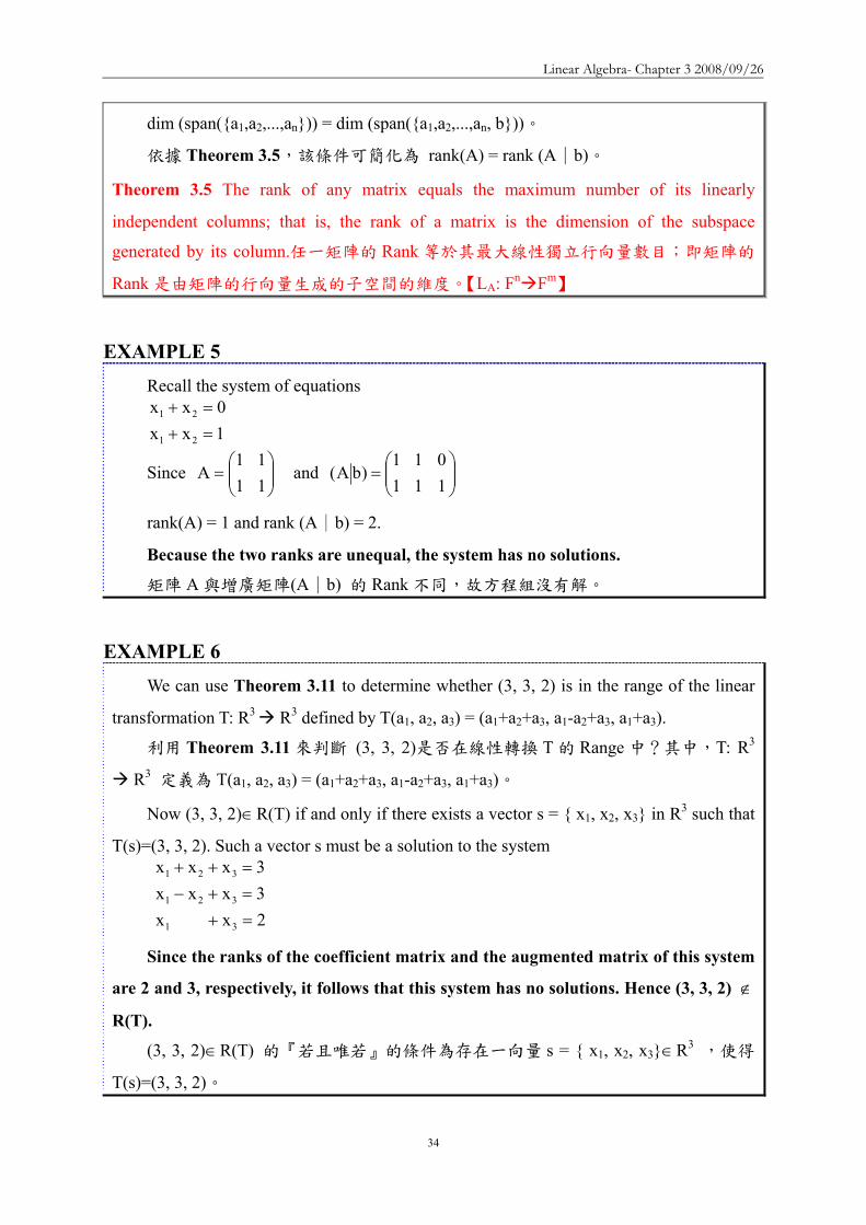
Linear Algebra- Chapter 3 20080926
35
向量 s 必須是 2xx3xxx3xxx
31
321
321
=+=+minus=++
的解
因係數矩陣⎟⎟⎟
⎠
⎞
⎜⎜⎜
⎝
⎛minus
101111111
的 Rank 為 2增廣矩陣⎟⎟⎟
⎠
⎞
⎜⎜⎜
⎝
⎛minus
233
101111111
的 Rank 為 3兩
者不相等故方程組無解(3 3 2) notin R(T)
Theorem 311 Let Ax = b be a system of linear equations Then the system is consistent
(相容)if and only if rank(A) = rank (A∣b) Matrix (A b) is called the ∣ augmented
matrix of the system Ax = b 令 Ax = b 為線性方程式方程組則此方程組至少有一個
解的『若且唯若』條件為 rank(A) = rank (A∣b) 矩陣(A∣b)稱為方程組 Ax = b 的
增廣矩陣
Application
In 1973 Wassily Leontief won the Nobel prize in economics for his work in developing
a mathematical model that can be used to describe various economic phenomena
1973 年Wassily Leontief 因研究一數學模式來描述各種經濟現象而獲頒諾貝爾經
濟獎
CLOSED MODEL
We begin by considering a simple society composed of three peoples (industries) ndash a
farmer who gows all the food a tailor who makes all the clothing and a carpenter who builds
all the housing We assume that each person sells to and buy from a central pool and that
everything produced is consumed Since no commodities either enter or leave the system this
case is referred to as the CLOSE MODEL
考慮一個單純社會的三種人生產食物的農夫製衣的裁縫師與蓋住屋的木匠
並假設採取集中聯營買賣且每一件產品皆付諸消費由於過程中沒有任何成品進入
或脫離這個系統所以稱為「封閉模式」
Each of these three individual consumes all three of the commodities produced in the
Linear Algebra- Chapter 3 20080926
36
society Suppose that the proportion of each of the commodities consumed by each person is
given in the following table
社會中每一位皆消費所生產的三種成品且每一種產品也都被三位所消費其消
費比例如下
食物 Food 衣物 Clothing 住屋 Housing
農夫 Farmer 040 020 020
裁縫師 Tailor 010 070 020
木匠 Carpenter 050 010 060
Let p1 p2 and p3 denote the incomes of the farmer tailor and carpenter respectively To
ensure that this society survives we require that the consumption of each individual equals
his or her income
令 p1p2 與 p3 分別表示農夫裁縫師與木匠的收入並為確保這個封閉社會可以
存活假設每一位的收入等於消費
Note that the farmer consumes 20 of the clothing Because the total cost of all clothing
is p2 the tailorrsquos income the amount spent by the farmer on clothing is 020 p2 Moreover the
amount spent by the farmer on food clothing and housing must equal the farmerrsquos income
and so we obtain the equation 040 p1 + 020 p2 + 030 p3 = p1
對農夫而言農夫的衣物消費佔 20然因所有衣物的消費總額 p2 等於裁縫師的
收入所以農夫在衣物上的消費為 020 p2且農夫在食物衣物與住屋的總消費要等
於農夫的收入 p1所以農夫的收入與消費關係式
040 p1 + 020 p2 + 020 p3 = p1
Similary equations describing the expenditures of the tailor and carpenter produce the
following system of linear equations
同理分別對裁縫師與木匠進行討論可獲得下列方程組
Linear Algebra- Chapter 3 20080926
37
040 p1 + 020 p2 + 020 p3 = p1
010 p1 + 070 p2 + 020 p3 = p2
050 p1 + 010 p2 + 060 p3 = p3
This system can be written as Ap = p
其中⎟⎟⎟
⎠
⎞
⎜⎜⎜
⎝
⎛=
3
2
1
ppp
p 且⎟⎟⎟
⎠
⎞
⎜⎜⎜
⎝
⎛=
600100500200700100200200400
A 稱為輸入-輸出(或消費)矩陣
(Input-output (or consumption) matrix)
Ap = p 稱為均衡條件(Equilibrium condition)
能否利用不等式 p ≦ p 來替代等式
At first it may seem reasonable to replace the equilibrium condition by the inequality
Ap ≦ p that is the requirement that consumption not exceed production But in fact Ap ≦ p implies that Ap = p in the closed model
For otherwise there exists a k for which
sumgt
jjkjk pAp
Hence since the columns of A sum to 1
sumsumsumsum ==gt
jj
i jjij
ii ppAp which is a contradiction (出現矛盾)
答案是在封閉系統中Ap ≦ p Ap = p
One solution to the homogeneous system (I ndash A) x = 0 which is equivalent to the
equilibrium condition is ⎟⎟⎟
⎠
⎞
⎜⎜⎜
⎝
⎛=
400350250
p
Linear Algebra- Chapter 3 20080926
38
齊次方程組(I ndash A) x = 0 或均衡條件的一個解為 ⎟⎟⎟
⎠
⎞
⎜⎜⎜
⎝
⎛=
400350250
p
We may interpret this to mean that the society survives if the farmer taior and carpenter
have incomes in the proportions 253540
⎟⎟⎟
⎠
⎞
⎜⎜⎜
⎝
⎛=
400350250
p 可以解釋為若農夫裁縫師與木匠收入比例為 253540則社會將
能生存下去
Theorem 312
Let A be an ntimesn input-output matrix having the form ⎟⎟⎠
⎞⎜⎜⎝
⎛=
EDCB
A where D is a 1times(n-
1) positive vector and C is an (n-1)times1 positive vector Then (I-A)x = 0 has a one-
dimensional solution set that is generated by a nonnegative vector
設 A 為 ntimesn 輸入-輸出矩陣 ⎟⎟⎠
⎞⎜⎜⎝
⎛=
EDCB
A 其中D 為 1times(n-1)正向量C 為
(n-1)times1 正向量則(I-A)x = 0 具有一維解集合且該解集合係由一非負向量所生成
Any input-output matrix with all positive entries satisfies the hypothesis of this theorem
任何輸入-輸出矩陣滿足 Theorem 312 的基本假設條件例如
⎟⎟⎟
⎠
⎞
⎜⎜⎜
⎝
⎛=
02502503502500650500750
A
OPEN MODEL
In the OPEN MODEL we assume that there is an outside demand for each of the
commodities produced Returning to our simple society let x1 x2 and x3 be the monetary
values of food clothing and housing produced with respective outside demands d1 d2 and d3
Let A be the 3times3 matrix such that Aij represents the amount of commodity i required to
Linear Algebra- Chapter 3 20080926
39
produce one monetary unit of commodity j Then the value of the surplus of food in the
society is x1 ndash (A11x1+A12x2+A13x3) that is the value of food produced minus the value of
food consumed while producing the three commodities The assumption that everything
produced is consumed gives us a similar equilibrium condition for the open model namely
that the surplus of each of the three commodities must equal the corresponding outside
demands Hence i
3
1jjiji dxAx =minussum
=
for j=1 2 3
在「開放模式」中我們假設每一產品皆有外來的需求在前述的單純社會裡
令 x1x2 與 x3 分別代表食物衣物與住屋的貨幣價值d1d2 與 d3 為食物衣物與住
屋的外來需求價值令 A 為 3times3 矩陣Aij 表示生產『一個貨幣單位』的產品 j 所需要
的產品 i 的價值於是此社會中食物的盈餘價值為 x1 ndash (A11x1+A12x2+A13x3)即食物的
價值減去生產食物衣物與住屋所需消耗的食物的價值意即生產出來的食物價值扣
掉用去生產食物衣物與住屋所消耗掉的價值)(A11A12A13 為生產一個貨幣單位
的食物 1衣物 2 與住屋 3 所需消耗的食物 1 數量A12x2 表示生產貨幣價值為 x2的衣物
所需要的食物價值)對每一種產品而言其盈餘價值等於外來的需求價值於是
i
3
1jjiji dxAx =minussum
=
for j=123
Suppose that 30 cents worth of food 10 cents worth of clothing and 30 cents worth of
housing are required for the production of $1 worth of food Similar suppose that 20 cents
worth of food 40 cents worth of clothing and 20 cents worth of housing are required for the
production of $1 worth of clothing Finally suppose that 30 cents worth of food 10 cents
worth of clothing and 30 cents worth of housing are required for the production of $1 worth
of housing Then the input-output matrix is
⎟⎟⎟
⎠
⎞
⎜⎜⎜
⎝
⎛=
300200300100400100300200300
A
假設生產價值 1 元的食物需要價值 30 分的食物(A11 = 03)價值 10 分的衣物
(A21 = 01)及價值 30 分的住屋(A31 = 03)生產價值 1 元的衣物需要價值 20 分的
食物(A12 = 02)價值 40 分的衣物(A22 = 04)及價值 20 分的住屋(A32 = 02)生
Linear Algebra- Chapter 3 20080926
40
產價值 1 元的住屋需要價值 30 分的食物(A13 = 03)價值 10 分的衣物(A23 = 01)
及價值 30 分的住屋(A33 = 03)於是輸入輸出矩陣 A 為
⎟⎟⎟
⎠
⎞
⎜⎜⎜
⎝
⎛=
300200300100400100300200300
A
若食物的外來需求值為 300 億元衣物為 200 億元住屋值為 1 百億元則
⎟⎟⎟
⎠
⎞
⎜⎜⎜
⎝
⎛=
⎟⎟⎟
⎠
⎞
⎜⎜⎜
⎝
⎛
⎟⎟⎟
⎠
⎞
⎜⎜⎜
⎝
⎛
minusminusminusminusminusminus
=minus=
minus
minus
700600900
100200300
700200300100600100300200300
d)AI(x
1
1
⎟⎟⎟
⎠
⎞
⎜⎜⎜
⎝
⎛=
700600900
x 表示要滿足外來需求必須生產的食物價值為 900 億元衣物價值為
600 億元住屋價值為 700 億元
Theorem
Let AX = Y be a system of n linear equations in n variables If Andash1 exists the
solution is unique and is given by X = Andash1Y
【Proof】
Substitute X = Andash1Y into the matrix equation
AX = A(Andash1Y) = (AAndash1)Y = InY = Y
The solution is unique
Let X1 be any solution thus AX1 = Y Multiplying both sides of this equation by Andash1
gives
Andash1AX1= Andash1Y InX1 = Andash1Y X1 = Andash1Y
Linear Algebra- Chapter 3 20080926
41
Example Example 1212
2x5x3x3x5x3x21x2x x
321
321
321
minus=++minus=minusminus=minusminus
⎥⎥⎥
⎦
⎤
⎢⎢⎢
⎣
⎡
minus=
⎥⎥⎥
⎦
⎤
⎢⎢⎢
⎣
⎡
⎥⎥⎥
⎦
⎤
⎢⎢⎢
⎣
⎡
minusminusminusminusminus
231
xxx
531532211
3
2
1
Solve the system of equations
This system can be written in the following matrix form
⎥⎥⎥
⎦
⎤
⎢⎢⎢
⎣
⎡
minus⎥⎥⎥
⎦
⎤
⎢⎢⎢
⎣
⎡
minusminusminusminusminus
=
⎥⎥⎥
⎦
⎤
⎢⎢⎢
⎣
⎡minus
231
531532211
xxx 1
3
2
1
If the matrix of coefficients is invertible the unique solutionIf the matrix of coefficients is invertible the unique solution isis
Example Example 2222
1 2 1 issolution unique The 321 =minus== xxx
⎥⎥⎥
⎦
⎤
⎢⎢⎢
⎣
⎡minus=
⎥⎥⎥
⎦
⎤
⎢⎢⎢
⎣
⎡
minus⎥⎥⎥
⎦
⎤
⎢⎢⎢
⎣
⎡
minusminusminus=
⎥⎥⎥
⎦
⎤
⎢⎢⎢
⎣
⎡
121
231
123135110
xxx
3
2
1
⎥⎥⎥
⎦
⎤
⎢⎢⎢
⎣
⎡
minusminusminus=
⎥⎥⎥
⎦
⎤
⎢⎢⎢
⎣
⎡
minusminusminusminusminus
=
minus
minus
123135110
531532211
A
1
1
The The LeontiefLeontief IO Model in IO Model in Economics Economics 1515
The Leontief input-output model is used to analyze the interdependence of economics Wassily Leontief received a Nobel Prize in 1973 for his work in thie fieldThe practical applications of this model have proliferated until it has now become a standard tool for investigating economic structures ranging from cities and corporation to states and countriesConsider an economics situation that involves ninterdependent industries The output of any one industry is needed as input by other industries and even possibly by the industry itself
The The LeontiefLeontief IO Model in IO Model in Economics Economics 2525
How a mathematical model involving a system of linear equations can be constructed to analyze such a situationAssume that each industry produces one commodity Let aij denote the amount of input of a certain commodity i to produce unit output of commodity j In our model let the amounts of input and output be measured in dollars Thus for example a34 = 045 means that 45 centsrsquo worth of commodity 3 is required to produce one dollarrsquos worth of commodity 4
The The LeontiefLeontief IO Model in IO Model in Economics Economics 3535
aij = amount of commodity i in one dollar of commodity jaij =生產一元價值的j產品需要耗用的i產品價值
The elements aij called input coefficients define a matrix A called the input-output matrix which describes the interdependence of the industriesExtending the model to include an open sector (all non-producing sectors) The product of industries may go not only into other producing industries but also into other non-producing sectors of the economy such as consumers and governments
The The LeontiefLeontief IO Model in IO Model in Economics Economics 4545
di = demand of the open sectors from industry ixi=total output of industry I necessary to meet demands of all n industries and the open sector
sectoropen of demand
nindustry of demand
2industry of demand
22
1industry of demand
11
industry ofoutput total
ininii
i
i dxaxaxax ++sdotsdotsdot++=
output ofportion sectoropen
output ofportion tryinterindusoutput total
DAXX +=Demand matrixDemand matrix
Output matrixOutput matrix
The The LeontiefLeontief IO Model in IO Model in Economics Economics 5555
Applying the model to the economy of a country X Applying the model to the economy of a country X represents the total output of each of the producing sectors represents the total output of each of the producing sectors of the economy and AX describes the contributions made of the economy and AX describes the contributions made by the various sectors to fulfilling the intersectional input by the various sectors to fulfilling the intersectional input requirements of the economyrequirements of the economyD is equal to (XD is equal to (X--AX) the difference between total output AX) the difference between total output X and industry transaction AXX and industry transaction AXD is thus the gross national product of the economyD is thus the gross national product of the economy
Example Example 1414
Consider an economy consisting of three industries having Consider an economy consisting of three industries having the following inputthe following input--output matrix output matrix AA Determine the output Determine the output levels required of the industries to meet the demands of levels required of the industries to meet the demands of the other industries and of the open sector in each casethe other industries and of the open sector in each case
in turn 321812
and 896
1612
9
5100
021
21
103
51
51
⎥⎥⎦
⎤
⎢⎢⎣
⎡
⎥⎥⎦
⎤
⎢⎢⎣
⎡
⎥⎥⎦
⎤
⎢⎢⎣
⎡=
⎥⎥⎥
⎦
⎤
⎢⎢⎢
⎣
⎡
= DA
The unit of The unit of DD are millions of dollarsare millions of dollars
Linear Algebra- Chapter 3 20080926
42
Example Example 2424
We wish to compute the output levels X that correspond to We wish to compute the output levels X that correspond to the various open sector demands D X is given by the the various open sector demands D X is given by the equation X = AX + D Rewritten as followsequation X = AX + D Rewritten as follows
X ndash AX = D rArr (I ndash A)X = D rArr X = (I ndash A) ndash1 D
⎥⎥⎥
⎦
⎤
⎢⎢⎢
⎣
⎡
=⎥⎥⎥
⎦
⎤
⎢⎢⎢
⎣
⎡
minus⎥⎥⎦
⎤
⎢⎢⎣
⎡=minus minus
minusminus
5400
021
21
103
51
54
5100
021
21
103
51
31
100010001
get We AI
⎥⎥⎥
⎦
⎤
⎢⎢⎢
⎣
⎡
=minus minus
4500
038
35
85
32
35
1)( AI
output ofingcorrespond valuesvarious
4500
038
35
85
32
35
)(
401020883957522133
32816189121269
)(
1
1
DAI
DAIX
minus
minus
minusuarruarruarruarruarruarruarr
⎥⎥⎦
⎤
⎢⎢⎣
⎡=
⎥⎥⎦
⎤
⎢⎢⎣
⎡
⎥⎥⎥
⎦
⎤
⎢⎢⎢
⎣
⎡
=minus=
Example Example 3434
By using Gauss-Jordan elimination
dollars of milliond are units The
40
15674
and 106629
209946
are 321812
and 896
1612
9
⎥⎥⎥
⎦
⎤
⎢⎢⎢
⎣
⎡
⎥⎥⎥
⎦
⎤
⎢⎢⎢
⎣
⎡
⎥⎥⎥
⎦
⎤
⎢⎢⎢
⎣
⎡
⎥⎥⎥
⎦
⎤
⎢⎢⎢
⎣
⎡
⎥⎥⎥
⎦
⎤
⎢⎢⎢
⎣
⎡
⎥⎥⎥
⎦
⎤
⎢⎢⎢
⎣
⎡
Example Example 4444
The output levels necessary to meet the demandsThe output levels necessary to meet the demands
IAAAIAI m =++++minus ))(( 2 L
mAAAIAI ++++=minus minus L21)(
Computing (IComputing (I--A) A) --11
1m
m2m2
m2
AI)AAAI(A)AAAI(I
)AAAI)(AI(
+minus=++++minus++++=
++++minusLL
L
NOTE 0A 1m rarr+
Population Movement Population Movement 1313
In 2000 58 million of people live in cities and 142 million of In 2000 58 million of people live in cities and 142 million of people people live in the surrounding suburbs Represent this information by tlive in the surrounding suburbs Represent this information by the he matrix matrix
The probability of a person staying in the city was 096 Thus tThe probability of a person staying in the city was 096 Thus the he probability of moving to the suburbs was 004 probability of moving to the suburbs was 004 The probability of a person moving to the city was 001 the The probability of a person moving to the city was 001 the probability of remaining in suburbia was 099probability of remaining in suburbia was 099
suburbcity
990040010960
suburbcity (to))from(
⎥⎦
⎤⎢⎣
⎡=P
⎥⎦
⎤⎢⎣
⎡=
14258
X0
City population in 2001 = people who remained from 2000 + peopleCity population in 2001 = people who remained from 2000 + peoplewho moved in from the suburbs = ( 096 who moved in from the suburbs = ( 096 timestimes 58 ) + (001 58 ) + (001 timestimes 142 ) = 142 ) = 571 million571 millionSuburban population in 2001 = people who moved in from the city Suburban population in 2001 = people who moved in from the city + people who stayed from 2000 = ( 004 + people who stayed from 2000 = ( 004 timestimes 58 ) + (099 58 ) + (099 timestimes 142 ) = 142 ) = 1429 million1429 millionCan arrive at these numbers using matrix multiplicationCan arrive at these numbers using matrix multiplication
⎥⎦
⎤⎢⎣
⎡=⎥
⎦
⎤⎢⎣
⎡⎥⎦
⎤⎢⎣
⎡==
9142157
14258
990040010960
PXX 01
Population Movement Population Movement 2323
Population Movement Population Movement 3333
Assume that the population flow represented by the matrix P is unchanged over the years The population distribution X2 after 2 years is given by X2 = P X1 = P2 X0 In general
Pn is called the n-step transition matrix The (ij)th element of Pngives the probability of going from state j to state i in n stepsFor example
in
ni XPX =+
suburbcity
960150040850
P
suburbcity (to))from(
4
⎥⎦
⎤⎢⎣
⎡=
The probability of living in the city in The probability of living in the city in 2000 and being in the suburbs 4 years 2000 and being in the suburbs 4 years later is 015later is 015
Markov ChainsMarkov Chains
The probabilities in the above model depend only on the The probabilities in the above model depend only on the current state of a person whether the person is living in the current state of a person whether the person is living in the city or in suburbiacity or in suburbiaThis type of model in which the probability of going from This type of model in which the probability of going from one state to another depends only on the current state one state to another depends only on the current state rather than on a more complete historical description is rather than on a more complete historical description is called a called a Markov chainMarkov chainMarkov chains are useful tools for scientists in many Markov chains are useful tools for scientists in many fields such as geneticsfields such as genetics
Linear Algebra- Chapter 3 20080926
43
GeneticsGenetics 1414
Genetics is the branch of biology that deals with Genetics is the branch of biology that deals with heredity heredity (遺傳)(遺傳) It is the study of units called It is the study of units called genes which determine the characteristics living genes which determine the characteristics living things inherit from their parents The inheritance things inherit from their parents The inheritance (遺傳)(遺傳)of such traitsof such traits(特徵)(特徵)as sex height eye as sex height eye color and hair color of human beings and such color and hair color of human beings and such traits as petaltraits as petal(花瓣)(花瓣) color and leaf shape of color and leaf shape of plants are governed by genesplants are governed by genesIn medicine agricultureIn medicine agriculturehelliphellip
GeneticsGenetics 2424
The traits of guinea pigsThe traits of guinea pigs(天竺鼠)(天竺鼠)are long hair and short hairare long hair and short hairThe length of hair is governed by a pair of gene which we denoteThe length of hair is governed by a pair of gene which we denote A A and aand aA guinea pig may have any one of the combination of AA A guinea pig may have any one of the combination of AA AaAa or or aaaa Each of these classes is called a genotypeEach of these classes is called a genotype(基因型)(基因型)The AA type guinea pig is indistinguishable in appearance from tThe AA type guinea pig is indistinguishable in appearance from the he AaAa type type ndashndash both have long hair both have long hair ndashndash whereas the whereas the aaaa type has short hairtype has short hairThe A gene is said to dominate the a geneThe A gene is said to dominate the a geneAn animal is called dominant An animal is called dominant (顯性)(顯性)if it has AA genes hybridif it has AA genes hybrid(混種)(混種) with with AaAa genes and recessive genes and recessive (隱性)(隱性)with with aaaa genesgenes
GeneticsGenetics 3434
When two guinea pigs are crossed the offspring inherits one genWhen two guinea pigs are crossed the offspring inherits one gene e from each parent in random mannerfrom each parent in random mannerGiven the genotype of the parents we can determine the Given the genotype of the parents we can determine the probabilities of the genotype of the offspringprobabilities of the genotype of the offspring
AA+AA AA+AA probabilities of AA probabilities of AA AaAa and and aaaa are 10and 0are 10and 0Aa+AAAa+AA probabilities of AA probabilities of AA AaAa and and aaaa are are frac12frac12 frac12frac12 and 0 and 0aa+AAaa+AA probabilities of AA probabilities of AA AaAa and and aaaa are 0 1 and 0are 0 1 and 0
This series of experiments is a Markov chain having transition This series of experiments is a Markov chain having transition matrixmatrix
aaAaAA
00012100211
P
aaAaAA
⎥⎥⎥
⎦
⎤
⎢⎢⎢
⎣
⎡=
GeneticsGenetics 4444
Assume an initial population of guinea pigs made up of an Assume an initial population of guinea pigs made up of an equal number of each genotypeequal number of each genotype
⎥⎥⎥
⎦
⎤
⎢⎢⎢
⎣
⎡=
313131
X0
The fractions of following generations are
⎥⎥⎥
⎦
⎤
⎢⎢⎢
⎣
⎡=
⎥⎥⎥
⎦
⎤
⎢⎢⎢
⎣
⎡=
⎥⎥⎥
⎦
⎤
⎢⎢⎢
⎣
⎡=
⎥⎥⎥
⎦
⎤
⎢⎢⎢
⎣
⎡=
01611615
X08187
X04143
X02121
X 4321
AAAAAaAaaaaa
3-4 Systems of Linear Equations ndash Computational Aspects
DEFINITION 36 Equivalent
Two systems of linear equations are called equivalent if they have the same solution
set
兩個線性方程組稱為等價意指兩者具有相同的解集合
Elementary Transformations Transformation called elementary transformations can be used to change a system of
linear equations into another system of linear equations that have the same solution
These transformations are used to solve system of linear equations by eliminating
variables
The equivalent transformations used in terms of matrix are called ELEMENTARY
ROW OPERATION
Linear Algebra- Chapter 3 20080926
44
Equivalent System Systems of equations that are related through elementary transformations are called
equivalent systems
Matrices that are related through elementary row operations are called row equivalent
matrices
The symbol asymp is used to indicate equivalence in both cases
Theorem 313 Let Ax = b be a system of m linear equations in n unknowns and let C be an invertible
mtimesm matrix Then the system (CA)x = Cb is equivalent to Ax = b
設 Ax = b 為含 n 個未知數m 個線性方程式的方程組若 C 為可逆的mtimesm
矩陣則(CA)x = Cb 等價於 Ax = b
【Proof】
Let K be the solution set for Ax = b and Krsquo the solution set for (CA)x = Cb If wisinK
then Aw = b So (CA)w = Cb and hence wisinKrsquo Thus KsubeKrsquo
Conversely if wisinKrsquo then (CA)w = Cb Hence Aw = C-1(CA)w = C-1(Cb) = b so
wisinK Thus KrsquosubeK and therefore K=Krsquo
設 K 為 Ax = b 的解集合且 Krsquo為(CA)x = Cb 的解集合
若 wisinK則 Aw = b (CA)w = Cb故 wisinKrsquo於是 KsubeKrsquo
反之若 wisinKrsquo則(CA)w = Cb Aw = C-1(CA)w = C-1(Cb) = b故 wisinK於是
KrsquosubeK因此K=Krsquo
Corollary Let Ax = b be a system of m linear equations in n unknowns If (Arsquo brsquo) is obtained ∣
from from (A b) by a finite number of elementary row operations then the system Arsquox = ∣
brsquo is equivalent to the original system
設 Ax = b 為含 n 個未知數m 個線性方程式的方程組若(Arsquo brsquo) ∣ 是由(A b) ∣
經過有限次數的基本列運算而得則 Arsquox = brsquo 等價於 Ax = b即兩者具有相同的解
集合
【Proof】
Suppose that (Arsquo brsquo) is obtained from (A b) by elementary row operations These ∣ ∣
Linear Algebra- Chapter 3 20080926
45
may be executed by multiplying (A b) by elementary mtimesm matrices E∣ 1 E2hellipEp Let
C=EphellipE2E1 then (Arsquo brsquo) = C(A b) = (CA Cb)∣ ∣ ∣
Since each Ei is invertible so is C Now Arsquo = CA and brsquo = Cb Thus by Theorem 313
the system Arsquox = brsquo is equivalent to the system Ax = b
設(Arsquo brsquo)∣ 是由(A b)∣ 經過基本列運算取得即以基本 mtimesm 矩陣 E1 E2hellipEp
乘上 (A b)∣ (Arsquo brsquo) = C(A b) = (CA Cb∣ ∣ ∣ )其中C=EphellipE2E1
因 Ei 可逆故 C 亦為可逆 Arsquo = CA 且 brsquo = Cb
依據 Theorem 313Arsquox = brsquo 等價於 Ax = b
Theorem 313 Let Ax = b be a system of m linear equations in n unknowns and let C be an
invertible mtimesm matrix Then the system (CA)x = Cb is equivalent to Ax = b 設 Ax = b
為含 n 個未知數m 個線性方程式的方程組若 C 為可逆的mtimesm 矩陣則(CA)x
= Cb 等價於 Ax = b
We now describe a method for solving any stystem of linear equations Consider for
example the system of linear equations
探討解線性方程組的方法hellip
2xxx2x3xxx1x2x3x2x3
4321
321
4321
=minus++=++=minus++
First we form the augmented matrix ⎟⎟⎟
⎠
⎞
⎜⎜⎜
⎝
⎛
minus
minus
231
112101112323
(增廣矩陣)
Interchanging the first and third rows ⎟⎟⎟
⎠
⎞
⎜⎜⎜
⎝
⎛
minus
minus
132
132301111121
(第 13 列互調)
Adding -1 times the first row to the second row and then add -3 times the first row to
the third row ⎟⎟⎟
⎠
⎞
⎜⎜⎜
⎝
⎛
minusminusminus
minus
512
104010101121
(第 1 列乘上 -1 加到第 2 列再以 -3 乘上
第 1 列加到第 3 列)
Linear Algebra- Chapter 3 20080926
46
Multiplying the second row by -1 ⎟⎟⎟
⎠
⎞
⎜⎜⎜
⎝
⎛
minusminus
minusminusminus
51
2
104010101121
(第 2 列乘上 -1)
Adding four times the second row to the third row ⎟⎟⎟
⎠
⎞
⎜⎜⎜
⎝
⎛
minusminus
minusminusminus
91
2
300010101121
(4 乘上第 2
列加到第 3 列)
Multiplying the third row by -13 ⎟⎟⎟
⎠
⎞
⎜⎜⎜
⎝
⎛minusminus
minus
31
2
100010101121
(第 3 列乘上 -13)
Adding the third row to the first and second rows to obtain zeros in row 1 column 4
and row 2 column 4 ⎟⎟⎟
⎠
⎞
⎜⎜⎜
⎝
⎛
325
100000100121
(將第 3 列加到第 1 列及第 2 列)
Adding -2 times the second row to the first row in order to make the first row second
column entry become zero ⎟⎟⎟
⎠
⎞
⎜⎜⎜
⎝
⎛
321
100000100101
(將第 2 列乘以 -2 再加至第 1 列)
We have now obtained the desired reduction of the augmented matrix
⎟⎟⎟
⎠
⎞
⎜⎜⎜
⎝
⎛
321
100000100101
是化簡後的增廣矩陣
This matrix corresponds to the system of linear equations
對應的線性方程組為
2x3x1xx
4
2
31
===+
By Corollary to Theorem 313 this system is equivalent to the original system But this
system is easily solved Obviously x2 = 2 and x4 = 3 Moreover x1 and x3 can be any values
Linear Algebra- Chapter 3 20080926
47
provided their sum is 1 Letting x3 = t we then have x1 = 1 ndash t Thus an arbitray solution to the
original system has the form
依據 Corollary to Theorem 313 化簡後的方程組與原方程組等值此方程組的解為
x2 = 3x4 = 3x1 + x3 = 1於是原方程組的任意解可以寫成
⎟⎟⎟⎟⎟
⎠
⎞
⎜⎜⎜⎜⎜
⎝
⎛minus
+
⎟⎟⎟⎟⎟
⎠
⎞
⎜⎜⎜⎜⎜
⎝
⎛
=
⎟⎟⎟⎟⎟
⎠
⎞
⎜⎜⎜⎜⎜
⎝
⎛ minus
0101
t
3021
3t2
t1
Observe that
⎪⎪⎭
⎪⎪⎬
⎫
⎪⎪⎩
⎪⎪⎨
⎧
⎟⎟⎟⎟⎟
⎠
⎞
⎜⎜⎜⎜⎜
⎝
⎛minus
0101
is a basis for the homogeneous system of equations
corresponding to the given system
其中
⎪⎪⎭
⎪⎪⎬
⎫
⎪⎪⎩
⎪⎪⎨
⎧
⎟⎟⎟⎟⎟
⎠
⎞
⎜⎜⎜⎜⎜
⎝
⎛minus
0101
是齊次方程組解集合的一組基底
Gauss-Jordan Elimination
Let A be an n times n matrix
1 Adjoin the identity n times n matrix In to A to form the matrix [A In]
2 Compute the reduced echelon form of [A In]
(1) If the reduced echelon form is of the type [In B] then B is the inverse of A
(2) If the reduced echelon form is not of the type [In B] in that the first n times n
submatrix is not In then A has no inverse
An n times n matrix A is invertible if and only if its reduced echelon form is In
DEFINITION 37 Reduced Row Echelon Form
A matrix is said to be in reduced row echelon form if the following three conditions
are satisfied
Linear Algebra- Chapter 3 20080926
48
一個矩陣可以被稱為簡約列梯形式必須具備有下列三條件
(a) Any row containing a nonzero entry preceeds any row in which all the entries are
zero (if any)
含有非零元素的任一列排在全含零元素的任一列前面(儘可能)
(b) The first nonzero entry in each row in the only nonzero entry in its column
各列中第一個非零元素為其所在行中唯一的非零元素
(c) The first nonzero entry in each row is 1 and it occurs in a column to thr right of the
first nonzero entry in the preceeding row
各列中第一個非零元素為 1 且它出現在前一列中第一個非零元素的右邊某一
行中
Reduced Echelon Form A matrix is in reduced echelon form if
1 Any rows consisting entirely of zeros are grouped at the bottom of the matrix
2 The first nonzero element of each other row is 1 This element is called a leading 1
3 The leading 1 of each row after the first is positioned to the right of the leading 1 of
the previous row
4 All other elements in a column that contains a leading 1 are zero
Theorem 314 Gaussian Elimination Transformation Gaussian elimination transform any matrix into its reduced row echelon form
利用 Gaussian elimination 將矩陣轉換成簡約列梯形式
We now describe a method for solving a system in which the augmented matrix is in
reduced row echelon form To illustrate this procedure we consider the system
14x8x3x2x2x28x5x2xxx6x3xxxx17x9x4xx3x2
54321
54321
54321
54321
=minus+++=minus+++=minus+++=minus+++
Linear Algebra- Chapter 3 20080926
49
for which the augmented matrix is
⎟⎟⎟⎟⎟
⎠
⎞
⎜⎜⎜⎜⎜
⎝
⎛
minusminusminusminus
1486
17
83222521113111194132
(增廣矩陣)
Applying Gaussian elimination to the augmented matrix of the system produces the
following sequence of matrices
利用 Gaussian elimination method 處理增廣矩陣
⎟⎟⎟⎟⎟
⎠
⎞
⎜⎜⎜⎜⎜
⎝
⎛
minusminusminusminus
1486
17
83222521113111194132
⎟⎟⎟⎟⎟
⎠
⎞
⎜⎜⎜⎜⎜
⎝
⎛
minusminusminusminus
148
176
83222521119413231111
⎟⎟⎟⎟⎟
⎠
⎞
⎜⎜⎜⎜⎜
⎝
⎛
minusminus
minus
0213
0000021000
1011020201
The system of linear equations corresponding to thus last matrix is
對應最後矩陣的線性方程組 2x2x
1xxx3x2x2x
54
532
531
=minus=+minus=minus+
Assign x3 = t1 x5 = t2
2t22x2x1tt1xxx
3t2t23x2x2x
254
21532
21531
+=+=+minus=+minus=
++minus=++minus=
Thus an arbitray solution s is of the form
於是任意解 s 具有下列形式
s =
⎟⎟⎟⎟⎟⎟
⎠
⎞
⎜⎜⎜⎜⎜⎜
⎝
⎛minus
+
⎟⎟⎟⎟⎟⎟
⎠
⎞
⎜⎜⎜⎜⎜⎜
⎝
⎛minus
+
⎟⎟⎟⎟⎟⎟
⎠
⎞
⎜⎜⎜⎜⎜⎜
⎝
⎛
=
⎟⎟⎟⎟⎟⎟
⎠
⎞
⎜⎜⎜⎜⎜⎜
⎝
⎛
+
+minus++minus
=
⎟⎟⎟⎟⎟⎟
⎠
⎞
⎜⎜⎜⎜⎜⎜
⎝
⎛
1201
2
t
00112
t
02013
t2t2
t1tt
3t2t2
xxxxx
21
2
2
1
21
21
5
4
3
2
1
where t1t2isinR
Linear Algebra- Chapter 3 20080926
50
Notice that
⎪⎪⎪
⎭
⎪⎪⎪
⎬
⎫
⎪⎪⎪
⎩
⎪⎪⎪
⎨
⎧
⎟⎟⎟⎟⎟⎟
⎠
⎞
⎜⎜⎜⎜⎜⎜
⎝
⎛minus
⎟⎟⎟⎟⎟⎟
⎠
⎞
⎜⎜⎜⎜⎜⎜
⎝
⎛minus
1201
2
00112
is a basis for the solution set of the corresponding
homogeneous system of equation and
⎟⎟⎟⎟⎟⎟
⎠
⎞
⎜⎜⎜⎜⎜⎜
⎝
⎛
02013
is a particular solution to the original system
⎪⎪⎪
⎭
⎪⎪⎪
⎬
⎫
⎪⎪⎪
⎩
⎪⎪⎪
⎨
⎧
⎟⎟⎟⎟⎟⎟
⎠
⎞
⎜⎜⎜⎜⎜⎜
⎝
⎛minus
⎟⎟⎟⎟⎟⎟
⎠
⎞
⎜⎜⎜⎜⎜⎜
⎝
⎛minus
1201
2
00112
是齊次方程組解集合的一組基底
⎟⎟⎟⎟⎟⎟
⎠
⎞
⎜⎜⎜⎜⎜⎜
⎝
⎛
02013
是原方程組的特別解
EXAMPLE 1
The matrix ⎟⎟⎟
⎠
⎞
⎜⎜⎜
⎝
⎛
101010011
is not in reduced row echelon form
因為第一行含有第一個非零元素在第一列但第一行尚含有其他非零元素
The matrix ⎟⎟⎟
⎠
⎞
⎜⎜⎜
⎝
⎛
110010012010
is not in reduced row echelon form
因為第一列第一個非零元素不在第一列第一個非零元素的右邊
The matrix ⎟⎟⎠
⎞⎜⎜⎝
⎛010002
is not in reduced row echelon form
因為第一列的第一個非零元素不是 1
Linear Algebra- Chapter 3 20080926
51
Reduced Echelon FormReduced Echelon Form
⎥⎥⎥
⎦
⎤
⎢⎢⎢
⎣
⎡
910030107001
⎥⎥⎥
⎦
⎤
⎢⎢⎢
⎣
⎡
100001000041
⎥⎥⎥
⎦
⎤
⎢⎢⎢
⎣
⎡
000210801
Not in Reduced Echelon Form
⎥⎥⎥
⎦
⎤
⎢⎢⎢
⎣
⎡
310000004021
⎥⎥⎥
⎦
⎤
⎢⎢⎢
⎣
⎡
100000430003021
⎥⎥⎥⎥
⎦
⎤
⎢⎢⎢⎢
⎣
⎡
0000210030108071
In Reduced Echelon Form
Use GaussUse Gauss--Jordan elimination to Jordan elimination to find reduced echelon formfind reduced echelon form 1313
Step 1 Interchange rows if necessary to bring a nonzero Step 1 Interchange rows if necessary to bring a nonzero element to the top of the first nonzero column This nonzero element to the top of the first nonzero column This nonzero element is called a pivotelement is called a pivot
⎥⎥⎦
⎤
⎢⎢⎣
⎡
minusminus
minus
1211244129333
22200
⎥⎥⎥
⎦
⎤
⎢⎢⎢
⎣
⎡
minusminus
minus
harrasymp
121124422200
129333
R2R1
Use GaussUse Gauss--Jordan elimination to Jordan elimination to find reduced echelon formfind reduced echelon form 2323
Step 2 Create a 1 in the pivot location by multiplying the Step 2 Create a 1 in the pivot location by multiplying the pivot row by 1pivotpivot row by 1pivot
Step 3 Create zero elsewhere in the pivot column by adding Step 3 Create zero elsewhere in the pivot column by adding suitable multiples of the pivot row to all other rows of the suitable multiples of the pivot row to all other rows of the matrixmatrix
⎥⎥⎥
⎦
⎤
⎢⎢⎢
⎣
⎡
minusminusminus
minus
minus+asymp
412002220043111
4)R1(R3
⎥⎥⎦
⎤
⎢⎢⎣
⎡
minusminus
minus
⎟⎠⎞
⎜⎝⎛asymp
12112442220043111
R13
1
The matrix is the reduced echelon form of the given matrixThe matrix is the reduced echelon form of the given matrix
Use GaussUse Gauss--Jordan elimination to Jordan elimination to find reduced echelon formfind reduced echelon form 3333
Step 4 Cover the pivot row and all rows above it Repeat Steps Step 4 Cover the pivot row and all rows above it Repeat Steps 1 1 and 2 for the remaining and 2 for the remaining submatrixsubmatrix Repeat Step 3 for the whole Repeat Step 3 for the whole matrix Continue until the reduced echelon form is reachedmatrix Continue until the reduced echelon form is reached
⎥⎥⎥
⎦
⎤
⎢⎢⎢
⎣
⎡
minusminus
+minus+asymp
⎥⎥⎥
⎦
⎤
⎢⎢⎢
⎣
⎡
minusminus
minus++asymp
⎥⎥⎥
⎦
⎤
⎢⎢⎢
⎣
⎡
minusminusminus
minus
⎟⎠⎞
⎜⎝⎛
asymp
⎥⎥⎥
⎦
⎤
⎢⎢⎢
⎣
⎡
minusminusminus
minus
6100050100
170011
R3R22)R3(R1
610001110052011
R2)2(R3R2R1
412001110043111
R221
412002220043111
Theorem 315 Let Ax = b be a system of r nonzero equations is in n unknown Suppose that rank(A)
= rank (A b)∣ and that (A b)∣ is in reduced row echelon form Then
設 Ax = b 為含有 n 個未知數r 個非零方程式的方程組假設 rank(A) = rank
(A b)∣ 且 (A b)∣ 為簡約列梯形式於是
(a) rank(A) = r
(b) If the general solution obtained by the procedure above is of the form s = s0 + t1u1
+ t2u2 +hellip+ tn-run-r then u1 u2hellip un-r is a basis for the solution set of the
corresponding homogeneous system and s0 is a solution to the original system 由
前述方法所得的 General solution 具有下列形式
s = s0 + t1u1 + t2u2 +hellip+ tn-run-r
其中u1 u2hellip un-r為齊次方程組 Ax = 0 的解集合的一組基底且 s0 為原方
程組的一個解)
【Proof】
Since (A b)∣ is in reduced row echelon form (A b)∣ must have r nonzero rows
Clearly these rows are linearly independent by the definition of the reduced row echelon
Linear Algebra- Chapter 3 20080926
52
form and so rank (A b)∣ = r Thus rank(A) = r
Let K be the solution set for Ax = b and let KH be the solution set for Ax = 0 Setting
t1 = t2 =hellip= tn-r = 0 we see that s = s0isinK But by Theorem 39 K = s +KH Hence
KH = - s0+K = span(u1 u2hellip un-r )
Because rank(A) = r we have dim(KH) = n-r Thus since dim(KH) = n-r and KH is
generated by a set u1 u2hellip un-r containing at most n-r vectors that is a basis for KH
由於(A b)∣ 具有簡約列梯形式因此(A b)∣ 必定具有 r 個非零列由簡約列梯形
式的定義得知 r 個非零列為線性獨立故 rank (A b)∣ = rrank(A) = r
令 K 為 Ax = b 的解集合 KH 為 Ax = 0 的解集合
假設 t1 = t2 =hellip= tn-r = 0(u1 u2hellip un-r非 KH的基底)則 s = s0isinK
依據 Theorem 39K = s +KH KH = - s0+K = span(u1 u2hellip un-r )
因 rank(A) = r所以 dim(KH) = n - r 且 KH 是由u1 u2hellip un-r 所生成
故原假設「t1 = t2 =hellip= tn-r = 0」不成立
因此 KH含有最多 n - r 個向量且這些向量為 KH的基底
Theorem 39 Let K be the solution set of a system of linear equations Ax = b and let KH be
the solution set of the corresponding homogeneous system Ax = 0 Then for any solution s
to Ax = b K =s + KH = s+k kisinKH 設 K 為線性方程組 Ax = b 的解集合且 KH
為對應的齊次方程組的解集合則對 Ax = b 的任一個解 s 而言K =s + KH = s+k
kisinKH
ExampleExampleSolve the system of equationsSolve the system of equations
7537429333
321
321
321
=minusminus=+minus=+minus
xxxxxxxxx
⎥⎥⎦
⎤
⎢⎢⎣
⎡
++asymp
000012104301
R2R3R2R1 12
431243
32
31
32
31+minus=+minus=rArr=+
=+rArr xxxx
xxxx
The general solution to the system isThe general solution to the system is
parameter) a (callednumber real is where 1243
3
2
1
rrxrxrx
=+minus=+minus=
⎥⎥⎥
⎦
⎤
⎢⎢⎢
⎣
⎡
minusminusminus
minus
minus+minus+asymp
⎥⎥⎥
⎦
⎤
⎢⎢⎢
⎣
⎡
minusminusminusminus
asymp
⎥⎥⎥
⎦
⎤
⎢⎢⎢
⎣
⎡
minusminusminusminus
242012103111
1R)3(3R1R)2(2R
715374123111
715374129333
R131
ExampleExample
Solve the system of equationsSolve the system of equations446942
1423258101242
4321
4321
4321
=minus+minusminus=+minus+minus
=minus+minus
xxxxxxxxxxxx
⎪⎪
⎩
⎪⎪
⎨
⎧
===
minus=
rArr==minus=minus
rArr
1x6xrx
2r2x
1x6x
2x2x
4
3
2
1
4
3
21
⎥⎥⎥
⎦
⎤
⎢⎢⎢
⎣
⎡ minusminusasymp
⎥⎥⎥
⎦
⎤
⎢⎢⎢
⎣
⎡minus
minusminusasymp
⎥⎥⎥
⎦
⎤
⎢⎢⎢
⎣
⎡
minusminusminusminusminusasymp
⎥⎥⎥
⎦
⎤
⎢⎢⎢
⎣
⎡
minusminusminusminusminusasymp
⎥⎥⎥
⎦
⎤
⎢⎢⎢
⎣
⎡
minusminusminusminusminus
minusminusasymp
⎥⎥⎥
⎦
⎤
⎢⎢⎢
⎣
⎡
minusminusminusminusminus
minusminus
+
minus+
+
minus+
minus+
+
110006010020021
110005110011021
14430051100
295621
2R31
144300153300295621
446942142321295621
44694214232158101242
R3R2
1)R3(R1
3R2R3
6)R2(R1
2)R1(R3
R1R2R1
21
Linear Algebra- Chapter 3 20080926
53
ExampleExampleSolve the system of equationsSolve the system of equations
432636242232
54321
54321
54321
=+minus+minusminus=++minus+=++minus+
xxxxxxxxxxxxxxx
⎥⎥⎦
⎤
⎢⎢⎣
⎡ minusasymp
⎥⎥⎦
⎤
⎢⎢⎣
⎡
minusminusminusminusminus
+
minus+
642000210000213121
431121636242213121
R1R3
2)R1(R2
⎥⎥⎦
⎤
⎢⎢⎣
⎡ minusasympharr 210000
642000213121
R3R2 ( ) ⎥⎥⎦
⎤
⎢⎢⎣
⎡ minusasymp
210000321000213121
2R21
⎥⎥⎦
⎤
⎢⎢⎣
⎡ minusminusminusasympminus+ 210000
321000750121
3)R2(R1 ⎥⎥⎦
⎤
⎢⎢⎣
⎡minus
minusasymp
minus+
+
210000101000300121
2)R3(R2
5R3R1
2x1x
3xx2x
5
4
321
=minus=
++minus=rArr
2xs and r somefor 1x sx rx
3sr2x
5
432
1
=minus===
++minus=
ExampleExample
Solve the system of Solve the system of equationsequations 122
32452232
32
321
321
321
=+minus=minus+
=+minus=+minus
xxxxxxxxxxx
⎥⎥
⎦
⎤
⎢⎢
⎣
⎡asymp
minusminusminus
minus
harr1220210063303211
R3R2
( ) ⎥⎥
⎦
⎤
⎢⎢
⎣
⎡asymp
minusminusminus
minus
1220210021103211
R231
⎥⎥
⎦
⎤
⎢⎢
⎣
⎡asympminusminusminus
minus+
+
5400210021101101
2)R2(R4
R2R1 ⎥⎥
⎦
⎤
⎢⎢
⎣
⎡asymp
minusminus
minus+
+
minus+
13000210040103001
4)R3R(R4
R3R2
1)R3(R1
( ) ⎥⎥
⎦
⎤
⎢⎢
⎣
⎡asymp
minusminus
1000210040103001
R4131
The system has no solutionThe system has no solution
⎥⎥
⎦
⎤
⎢⎢
⎣
⎡asymp
⎥⎥
⎦
⎤
⎢⎢
⎣
⎡
minusminusminus
minus
minusminusminusminus
minus+
minus+
1220633021003211
1220312145223211
1)R1(R3
2)R1(R2
0x1+0x2+0x3=1
Curve FittingCurve Fitting
A set of data points A set of data points is given and it is is given and it is necessary to find a polynomial whose graph passes through the necessary to find a polynomial whose graph passes through the points points The points are often measurements in an experiment The points are often measurements in an experiment The xThe x--coordinates are called coordinates are called base pointsbase pointsIt can be shown that if the base points are all distinct then aIt can be shown that if the base points are all distinct then a unique unique polynomial of degree n polynomial of degree n ndashndash 1 (or less)1 (or less)
can be fitted to thecan be fitted to the pointspoints
) ( ) ( ) ( 2211 nn yxyxyx K
11
2210
minusminus
minusminus ++++= n
nn
n xaxaxaay K
The coefficients can be found by substituting the points The coefficients can be found by substituting the points into the polynomial equation and then solving a system into the polynomial equation and then solving a system of linear equationsof linear equations
ExampleExample
Determine the equation of the polynomial of degree 2 whose graphpasses through the points (1 6) (2 3) (3 2)
Let the polynomial be and substituting x = 1 y = 6 x = 2 y = 3 x = 3 y = 2 we have
Solving this system for a0 a1 and a2 using Gauss-Jordan elimination
⎥⎥⎥
⎦
⎤
⎢⎢⎢
⎣
⎡minus
minus
minus+minus+asymp
220033109201
1)R2(R31)R2(R1
2210 xaxaay ++=
2a9a3a3a4a2a6aaa
210
210
210
=++=++=++
⎥⎥⎥
⎦
⎤
⎢⎢⎢
⎣
⎡
minusminus
⎥⎥⎥
⎦
⎤
⎢⎢⎢
⎣
⎡
minus+minus+asymp
482033106111
293134216111
1)R1(R31)R1(R2
( )⎥⎥⎥
⎦
⎤
⎢⎢⎢
⎣
⎡minus
⎥⎥⎥
⎦
⎤
⎢⎢⎢
⎣
⎡minus
minusasymp
minus++asymp
11006010
11001
110033109201
3)R3(R22R3R1
R321
We get a0 = 11 a1 = ndash 6 a2 = 1The parabola that passes through these points is y = 11 ndash 6x + x2
ExampleExample Traffic FlowTraffic Flow
Network analysis plays an important role in electrical Network analysis plays an important role in electrical engineeringengineeringThe concepts and tools of network analysis have been The concepts and tools of network analysis have been found to be useful in many other fields such as found to be useful in many other fields such as information theory and the study of transportation systemsinformation theory and the study of transportation systemsThe analysis of traffic flow through a road network during The analysis of traffic flow through a road network during peak period illustrates how systems of linear equations peak period illustrates how systems of linear equations with with manymany solutions can arise in practicesolutions can arise in practice
Traffic FlowTraffic Flow
Consider the typical road network The streets are all oneConsider the typical road network The streets are all one--way with the arrows indicating the direction of traffic flowway with the arrows indicating the direction of traffic flowThe flow of traffic in and out of the network is measured The flow of traffic in and out of the network is measured in vehicles per hour (in vehicles per hour (vphvph))How to construct a mathematical model to analyze this How to construct a mathematical model to analyze this network network
Traffic Traffic FlowFlowTRAFFIC LAWTRAFFIC LAWhelliphellipAll traffic entering an intersection must leave that All traffic entering an intersection must leave that intersectionintersection
Linear Algebra- Chapter 3 20080926
54
Junction AJunction BJunction CJunction DJunction EJunction F 600
800 200 500 100 600
54
643
73
72
621
51
=+=++minus=+minus=minus=+minus=+
xxxxx
xxxx
xxxxx
⎥⎥⎥⎥⎥⎥⎥⎥⎥⎥⎥⎥⎥
⎦
⎤
⎢⎢⎢⎢⎢⎢⎢⎢⎢⎢⎢⎢⎢
⎣
⎡
asympasymp
⎥⎥⎥⎥⎥⎥⎥⎥⎥⎥⎥⎥⎥
⎦
⎤
⎢⎢⎢⎢⎢⎢⎢⎢⎢⎢⎢⎢⎢
⎣
⎡
minusminus
minusminusminusminus
minusminus
minusminus
0000000001110000
6001101000200100010050010000106001100001
600001100080001011002001000100500100001010001000116000010001
L
Traffic FlowTraffic FlowJunction AJunction BJunction CJunction DJunction EJunction F 600
800 200 500 100 600
54
643
73
72
621
51
=+=++minus=+minus=minus=+minus=+
xxxxx
xxxx
xxxxx
Perform road work on x7 Because x3 ge 0 the minimum flow 200 in the branch x7 can be obtained by making x3 = 0 (closing DE to traffic)
Traffic FlowTraffic Flow
We get
765
76473
72761
xx x600xxx200x x500x x600xxx
minus=++minus=minus=+=+minusminus=

Linear Algebra- Chapter 3 20080926
37
040 p1 + 020 p2 + 020 p3 = p1
010 p1 + 070 p2 + 020 p3 = p2
050 p1 + 010 p2 + 060 p3 = p3
This system can be written as Ap = p
其中⎟⎟⎟
⎠
⎞
⎜⎜⎜
⎝
⎛=
3
2
1
ppp
p 且⎟⎟⎟
⎠
⎞
⎜⎜⎜
⎝
⎛=
600100500200700100200200400
A 稱為輸入-輸出(或消費)矩陣
(Input-output (or consumption) matrix)
Ap = p 稱為均衡條件(Equilibrium condition)
能否利用不等式 p ≦ p 來替代等式
At first it may seem reasonable to replace the equilibrium condition by the inequality
Ap ≦ p that is the requirement that consumption not exceed production But in fact Ap ≦ p implies that Ap = p in the closed model
For otherwise there exists a k for which
sumgt
jjkjk pAp
Hence since the columns of A sum to 1
sumsumsumsum ==gt
jj
i jjij
ii ppAp which is a contradiction (出現矛盾)
答案是在封閉系統中Ap ≦ p Ap = p
One solution to the homogeneous system (I ndash A) x = 0 which is equivalent to the
equilibrium condition is ⎟⎟⎟
⎠
⎞
⎜⎜⎜
⎝
⎛=
400350250
p
Linear Algebra- Chapter 3 20080926
38
齊次方程組(I ndash A) x = 0 或均衡條件的一個解為 ⎟⎟⎟
⎠
⎞
⎜⎜⎜
⎝
⎛=
400350250
p
We may interpret this to mean that the society survives if the farmer taior and carpenter
have incomes in the proportions 253540
⎟⎟⎟
⎠
⎞
⎜⎜⎜
⎝
⎛=
400350250
p 可以解釋為若農夫裁縫師與木匠收入比例為 253540則社會將
能生存下去
Theorem 312
Let A be an ntimesn input-output matrix having the form ⎟⎟⎠
⎞⎜⎜⎝
⎛=
EDCB
A where D is a 1times(n-
1) positive vector and C is an (n-1)times1 positive vector Then (I-A)x = 0 has a one-
dimensional solution set that is generated by a nonnegative vector
設 A 為 ntimesn 輸入-輸出矩陣 ⎟⎟⎠
⎞⎜⎜⎝
⎛=
EDCB
A 其中D 為 1times(n-1)正向量C 為
(n-1)times1 正向量則(I-A)x = 0 具有一維解集合且該解集合係由一非負向量所生成
Any input-output matrix with all positive entries satisfies the hypothesis of this theorem
任何輸入-輸出矩陣滿足 Theorem 312 的基本假設條件例如
⎟⎟⎟
⎠
⎞
⎜⎜⎜
⎝
⎛=
02502503502500650500750
A
OPEN MODEL
In the OPEN MODEL we assume that there is an outside demand for each of the
commodities produced Returning to our simple society let x1 x2 and x3 be the monetary
values of food clothing and housing produced with respective outside demands d1 d2 and d3
Let A be the 3times3 matrix such that Aij represents the amount of commodity i required to
Linear Algebra- Chapter 3 20080926
39
produce one monetary unit of commodity j Then the value of the surplus of food in the
society is x1 ndash (A11x1+A12x2+A13x3) that is the value of food produced minus the value of
food consumed while producing the three commodities The assumption that everything
produced is consumed gives us a similar equilibrium condition for the open model namely
that the surplus of each of the three commodities must equal the corresponding outside
demands Hence i
3
1jjiji dxAx =minussum
=
for j=1 2 3
在「開放模式」中我們假設每一產品皆有外來的需求在前述的單純社會裡
令 x1x2 與 x3 分別代表食物衣物與住屋的貨幣價值d1d2 與 d3 為食物衣物與住
屋的外來需求價值令 A 為 3times3 矩陣Aij 表示生產『一個貨幣單位』的產品 j 所需要
的產品 i 的價值於是此社會中食物的盈餘價值為 x1 ndash (A11x1+A12x2+A13x3)即食物的
價值減去生產食物衣物與住屋所需消耗的食物的價值意即生產出來的食物價值扣
掉用去生產食物衣物與住屋所消耗掉的價值)(A11A12A13 為生產一個貨幣單位
的食物 1衣物 2 與住屋 3 所需消耗的食物 1 數量A12x2 表示生產貨幣價值為 x2的衣物
所需要的食物價值)對每一種產品而言其盈餘價值等於外來的需求價值於是
i
3
1jjiji dxAx =minussum
=
for j=123
Suppose that 30 cents worth of food 10 cents worth of clothing and 30 cents worth of
housing are required for the production of $1 worth of food Similar suppose that 20 cents
worth of food 40 cents worth of clothing and 20 cents worth of housing are required for the
production of $1 worth of clothing Finally suppose that 30 cents worth of food 10 cents
worth of clothing and 30 cents worth of housing are required for the production of $1 worth
of housing Then the input-output matrix is
⎟⎟⎟
⎠
⎞
⎜⎜⎜
⎝
⎛=
300200300100400100300200300
A
假設生產價值 1 元的食物需要價值 30 分的食物(A11 = 03)價值 10 分的衣物
(A21 = 01)及價值 30 分的住屋(A31 = 03)生產價值 1 元的衣物需要價值 20 分的
食物(A12 = 02)價值 40 分的衣物(A22 = 04)及價值 20 分的住屋(A32 = 02)生
Linear Algebra- Chapter 3 20080926
40
產價值 1 元的住屋需要價值 30 分的食物(A13 = 03)價值 10 分的衣物(A23 = 01)
及價值 30 分的住屋(A33 = 03)於是輸入輸出矩陣 A 為
⎟⎟⎟
⎠
⎞
⎜⎜⎜
⎝
⎛=
300200300100400100300200300
A
若食物的外來需求值為 300 億元衣物為 200 億元住屋值為 1 百億元則
⎟⎟⎟
⎠
⎞
⎜⎜⎜
⎝
⎛=
⎟⎟⎟
⎠
⎞
⎜⎜⎜
⎝
⎛
⎟⎟⎟
⎠
⎞
⎜⎜⎜
⎝
⎛
minusminusminusminusminusminus
=minus=
minus
minus
700600900
100200300
700200300100600100300200300
d)AI(x
1
1
⎟⎟⎟
⎠
⎞
⎜⎜⎜
⎝
⎛=
700600900
x 表示要滿足外來需求必須生產的食物價值為 900 億元衣物價值為
600 億元住屋價值為 700 億元
Theorem
Let AX = Y be a system of n linear equations in n variables If Andash1 exists the
solution is unique and is given by X = Andash1Y
【Proof】
Substitute X = Andash1Y into the matrix equation
AX = A(Andash1Y) = (AAndash1)Y = InY = Y
The solution is unique
Let X1 be any solution thus AX1 = Y Multiplying both sides of this equation by Andash1
gives
Andash1AX1= Andash1Y InX1 = Andash1Y X1 = Andash1Y
Linear Algebra- Chapter 3 20080926
41
Example Example 1212
2x5x3x3x5x3x21x2x x
321
321
321
minus=++minus=minusminus=minusminus
⎥⎥⎥
⎦
⎤
⎢⎢⎢
⎣
⎡
minus=
⎥⎥⎥
⎦
⎤
⎢⎢⎢
⎣
⎡
⎥⎥⎥
⎦
⎤
⎢⎢⎢
⎣
⎡
minusminusminusminusminus
231
xxx
531532211
3
2
1
Solve the system of equations
This system can be written in the following matrix form
⎥⎥⎥
⎦
⎤
⎢⎢⎢
⎣
⎡
minus⎥⎥⎥
⎦
⎤
⎢⎢⎢
⎣
⎡
minusminusminusminusminus
=
⎥⎥⎥
⎦
⎤
⎢⎢⎢
⎣
⎡minus
231
531532211
xxx 1
3
2
1
If the matrix of coefficients is invertible the unique solutionIf the matrix of coefficients is invertible the unique solution isis
Example Example 2222
1 2 1 issolution unique The 321 =minus== xxx
⎥⎥⎥
⎦
⎤
⎢⎢⎢
⎣
⎡minus=
⎥⎥⎥
⎦
⎤
⎢⎢⎢
⎣
⎡
minus⎥⎥⎥
⎦
⎤
⎢⎢⎢
⎣
⎡
minusminusminus=
⎥⎥⎥
⎦
⎤
⎢⎢⎢
⎣
⎡
121
231
123135110
xxx
3
2
1
⎥⎥⎥
⎦
⎤
⎢⎢⎢
⎣
⎡
minusminusminus=
⎥⎥⎥
⎦
⎤
⎢⎢⎢
⎣
⎡
minusminusminusminusminus
=
minus
minus
123135110
531532211
A
1
1
The The LeontiefLeontief IO Model in IO Model in Economics Economics 1515
The Leontief input-output model is used to analyze the interdependence of economics Wassily Leontief received a Nobel Prize in 1973 for his work in thie fieldThe practical applications of this model have proliferated until it has now become a standard tool for investigating economic structures ranging from cities and corporation to states and countriesConsider an economics situation that involves ninterdependent industries The output of any one industry is needed as input by other industries and even possibly by the industry itself
The The LeontiefLeontief IO Model in IO Model in Economics Economics 2525
How a mathematical model involving a system of linear equations can be constructed to analyze such a situationAssume that each industry produces one commodity Let aij denote the amount of input of a certain commodity i to produce unit output of commodity j In our model let the amounts of input and output be measured in dollars Thus for example a34 = 045 means that 45 centsrsquo worth of commodity 3 is required to produce one dollarrsquos worth of commodity 4
The The LeontiefLeontief IO Model in IO Model in Economics Economics 3535
aij = amount of commodity i in one dollar of commodity jaij =生產一元價值的j產品需要耗用的i產品價值
The elements aij called input coefficients define a matrix A called the input-output matrix which describes the interdependence of the industriesExtending the model to include an open sector (all non-producing sectors) The product of industries may go not only into other producing industries but also into other non-producing sectors of the economy such as consumers and governments
The The LeontiefLeontief IO Model in IO Model in Economics Economics 4545
di = demand of the open sectors from industry ixi=total output of industry I necessary to meet demands of all n industries and the open sector
sectoropen of demand
nindustry of demand
2industry of demand
22
1industry of demand
11
industry ofoutput total
ininii
i
i dxaxaxax ++sdotsdotsdot++=
output ofportion sectoropen
output ofportion tryinterindusoutput total
DAXX +=Demand matrixDemand matrix
Output matrixOutput matrix
The The LeontiefLeontief IO Model in IO Model in Economics Economics 5555
Applying the model to the economy of a country X Applying the model to the economy of a country X represents the total output of each of the producing sectors represents the total output of each of the producing sectors of the economy and AX describes the contributions made of the economy and AX describes the contributions made by the various sectors to fulfilling the intersectional input by the various sectors to fulfilling the intersectional input requirements of the economyrequirements of the economyD is equal to (XD is equal to (X--AX) the difference between total output AX) the difference between total output X and industry transaction AXX and industry transaction AXD is thus the gross national product of the economyD is thus the gross national product of the economy
Example Example 1414
Consider an economy consisting of three industries having Consider an economy consisting of three industries having the following inputthe following input--output matrix output matrix AA Determine the output Determine the output levels required of the industries to meet the demands of levels required of the industries to meet the demands of the other industries and of the open sector in each casethe other industries and of the open sector in each case
in turn 321812
and 896
1612
9
5100
021
21
103
51
51
⎥⎥⎦
⎤
⎢⎢⎣
⎡
⎥⎥⎦
⎤
⎢⎢⎣
⎡
⎥⎥⎦
⎤
⎢⎢⎣
⎡=
⎥⎥⎥
⎦
⎤
⎢⎢⎢
⎣
⎡
= DA
The unit of The unit of DD are millions of dollarsare millions of dollars
Linear Algebra- Chapter 3 20080926
42
Example Example 2424
We wish to compute the output levels X that correspond to We wish to compute the output levels X that correspond to the various open sector demands D X is given by the the various open sector demands D X is given by the equation X = AX + D Rewritten as followsequation X = AX + D Rewritten as follows
X ndash AX = D rArr (I ndash A)X = D rArr X = (I ndash A) ndash1 D
⎥⎥⎥
⎦
⎤
⎢⎢⎢
⎣
⎡
=⎥⎥⎥
⎦
⎤
⎢⎢⎢
⎣
⎡
minus⎥⎥⎦
⎤
⎢⎢⎣
⎡=minus minus
minusminus
5400
021
21
103
51
54
5100
021
21
103
51
31
100010001
get We AI
⎥⎥⎥
⎦
⎤
⎢⎢⎢
⎣
⎡
=minus minus
4500
038
35
85
32
35
1)( AI
output ofingcorrespond valuesvarious
4500
038
35
85
32
35
)(
401020883957522133
32816189121269
)(
1
1
DAI
DAIX
minus
minus
minusuarruarruarruarruarruarruarr
⎥⎥⎦
⎤
⎢⎢⎣
⎡=
⎥⎥⎦
⎤
⎢⎢⎣
⎡
⎥⎥⎥
⎦
⎤
⎢⎢⎢
⎣
⎡
=minus=
Example Example 3434
By using Gauss-Jordan elimination
dollars of milliond are units The
40
15674
and 106629
209946
are 321812
and 896
1612
9
⎥⎥⎥
⎦
⎤
⎢⎢⎢
⎣
⎡
⎥⎥⎥
⎦
⎤
⎢⎢⎢
⎣
⎡
⎥⎥⎥
⎦
⎤
⎢⎢⎢
⎣
⎡
⎥⎥⎥
⎦
⎤
⎢⎢⎢
⎣
⎡
⎥⎥⎥
⎦
⎤
⎢⎢⎢
⎣
⎡
⎥⎥⎥
⎦
⎤
⎢⎢⎢
⎣
⎡
Example Example 4444
The output levels necessary to meet the demandsThe output levels necessary to meet the demands
IAAAIAI m =++++minus ))(( 2 L
mAAAIAI ++++=minus minus L21)(
Computing (IComputing (I--A) A) --11
1m
m2m2
m2
AI)AAAI(A)AAAI(I
)AAAI)(AI(
+minus=++++minus++++=
++++minusLL
L
NOTE 0A 1m rarr+
Population Movement Population Movement 1313
In 2000 58 million of people live in cities and 142 million of In 2000 58 million of people live in cities and 142 million of people people live in the surrounding suburbs Represent this information by tlive in the surrounding suburbs Represent this information by the he matrix matrix
The probability of a person staying in the city was 096 Thus tThe probability of a person staying in the city was 096 Thus the he probability of moving to the suburbs was 004 probability of moving to the suburbs was 004 The probability of a person moving to the city was 001 the The probability of a person moving to the city was 001 the probability of remaining in suburbia was 099probability of remaining in suburbia was 099
suburbcity
990040010960
suburbcity (to))from(
⎥⎦
⎤⎢⎣
⎡=P
⎥⎦
⎤⎢⎣
⎡=
14258
X0
City population in 2001 = people who remained from 2000 + peopleCity population in 2001 = people who remained from 2000 + peoplewho moved in from the suburbs = ( 096 who moved in from the suburbs = ( 096 timestimes 58 ) + (001 58 ) + (001 timestimes 142 ) = 142 ) = 571 million571 millionSuburban population in 2001 = people who moved in from the city Suburban population in 2001 = people who moved in from the city + people who stayed from 2000 = ( 004 + people who stayed from 2000 = ( 004 timestimes 58 ) + (099 58 ) + (099 timestimes 142 ) = 142 ) = 1429 million1429 millionCan arrive at these numbers using matrix multiplicationCan arrive at these numbers using matrix multiplication
⎥⎦
⎤⎢⎣
⎡=⎥
⎦
⎤⎢⎣
⎡⎥⎦
⎤⎢⎣
⎡==
9142157
14258
990040010960
PXX 01
Population Movement Population Movement 2323
Population Movement Population Movement 3333
Assume that the population flow represented by the matrix P is unchanged over the years The population distribution X2 after 2 years is given by X2 = P X1 = P2 X0 In general
Pn is called the n-step transition matrix The (ij)th element of Pngives the probability of going from state j to state i in n stepsFor example
in
ni XPX =+
suburbcity
960150040850
P
suburbcity (to))from(
4
⎥⎦
⎤⎢⎣
⎡=
The probability of living in the city in The probability of living in the city in 2000 and being in the suburbs 4 years 2000 and being in the suburbs 4 years later is 015later is 015
Markov ChainsMarkov Chains
The probabilities in the above model depend only on the The probabilities in the above model depend only on the current state of a person whether the person is living in the current state of a person whether the person is living in the city or in suburbiacity or in suburbiaThis type of model in which the probability of going from This type of model in which the probability of going from one state to another depends only on the current state one state to another depends only on the current state rather than on a more complete historical description is rather than on a more complete historical description is called a called a Markov chainMarkov chainMarkov chains are useful tools for scientists in many Markov chains are useful tools for scientists in many fields such as geneticsfields such as genetics
Linear Algebra- Chapter 3 20080926
43
GeneticsGenetics 1414
Genetics is the branch of biology that deals with Genetics is the branch of biology that deals with heredity heredity (遺傳)(遺傳) It is the study of units called It is the study of units called genes which determine the characteristics living genes which determine the characteristics living things inherit from their parents The inheritance things inherit from their parents The inheritance (遺傳)(遺傳)of such traitsof such traits(特徵)(特徵)as sex height eye as sex height eye color and hair color of human beings and such color and hair color of human beings and such traits as petaltraits as petal(花瓣)(花瓣) color and leaf shape of color and leaf shape of plants are governed by genesplants are governed by genesIn medicine agricultureIn medicine agriculturehelliphellip
GeneticsGenetics 2424
The traits of guinea pigsThe traits of guinea pigs(天竺鼠)(天竺鼠)are long hair and short hairare long hair and short hairThe length of hair is governed by a pair of gene which we denoteThe length of hair is governed by a pair of gene which we denote A A and aand aA guinea pig may have any one of the combination of AA A guinea pig may have any one of the combination of AA AaAa or or aaaa Each of these classes is called a genotypeEach of these classes is called a genotype(基因型)(基因型)The AA type guinea pig is indistinguishable in appearance from tThe AA type guinea pig is indistinguishable in appearance from the he AaAa type type ndashndash both have long hair both have long hair ndashndash whereas the whereas the aaaa type has short hairtype has short hairThe A gene is said to dominate the a geneThe A gene is said to dominate the a geneAn animal is called dominant An animal is called dominant (顯性)(顯性)if it has AA genes hybridif it has AA genes hybrid(混種)(混種) with with AaAa genes and recessive genes and recessive (隱性)(隱性)with with aaaa genesgenes
GeneticsGenetics 3434
When two guinea pigs are crossed the offspring inherits one genWhen two guinea pigs are crossed the offspring inherits one gene e from each parent in random mannerfrom each parent in random mannerGiven the genotype of the parents we can determine the Given the genotype of the parents we can determine the probabilities of the genotype of the offspringprobabilities of the genotype of the offspring
AA+AA AA+AA probabilities of AA probabilities of AA AaAa and and aaaa are 10and 0are 10and 0Aa+AAAa+AA probabilities of AA probabilities of AA AaAa and and aaaa are are frac12frac12 frac12frac12 and 0 and 0aa+AAaa+AA probabilities of AA probabilities of AA AaAa and and aaaa are 0 1 and 0are 0 1 and 0
This series of experiments is a Markov chain having transition This series of experiments is a Markov chain having transition matrixmatrix
aaAaAA
00012100211
P
aaAaAA
⎥⎥⎥
⎦
⎤
⎢⎢⎢
⎣
⎡=
GeneticsGenetics 4444
Assume an initial population of guinea pigs made up of an Assume an initial population of guinea pigs made up of an equal number of each genotypeequal number of each genotype
⎥⎥⎥
⎦
⎤
⎢⎢⎢
⎣
⎡=
313131
X0
The fractions of following generations are
⎥⎥⎥
⎦
⎤
⎢⎢⎢
⎣
⎡=
⎥⎥⎥
⎦
⎤
⎢⎢⎢
⎣
⎡=
⎥⎥⎥
⎦
⎤
⎢⎢⎢
⎣
⎡=
⎥⎥⎥
⎦
⎤
⎢⎢⎢
⎣
⎡=
01611615
X08187
X04143
X02121
X 4321
AAAAAaAaaaaa
3-4 Systems of Linear Equations ndash Computational Aspects
DEFINITION 36 Equivalent
Two systems of linear equations are called equivalent if they have the same solution
set
兩個線性方程組稱為等價意指兩者具有相同的解集合
Elementary Transformations Transformation called elementary transformations can be used to change a system of
linear equations into another system of linear equations that have the same solution
These transformations are used to solve system of linear equations by eliminating
variables
The equivalent transformations used in terms of matrix are called ELEMENTARY
ROW OPERATION
Linear Algebra- Chapter 3 20080926
44
Equivalent System Systems of equations that are related through elementary transformations are called
equivalent systems
Matrices that are related through elementary row operations are called row equivalent
matrices
The symbol asymp is used to indicate equivalence in both cases
Theorem 313 Let Ax = b be a system of m linear equations in n unknowns and let C be an invertible
mtimesm matrix Then the system (CA)x = Cb is equivalent to Ax = b
設 Ax = b 為含 n 個未知數m 個線性方程式的方程組若 C 為可逆的mtimesm
矩陣則(CA)x = Cb 等價於 Ax = b
【Proof】
Let K be the solution set for Ax = b and Krsquo the solution set for (CA)x = Cb If wisinK
then Aw = b So (CA)w = Cb and hence wisinKrsquo Thus KsubeKrsquo
Conversely if wisinKrsquo then (CA)w = Cb Hence Aw = C-1(CA)w = C-1(Cb) = b so
wisinK Thus KrsquosubeK and therefore K=Krsquo
設 K 為 Ax = b 的解集合且 Krsquo為(CA)x = Cb 的解集合
若 wisinK則 Aw = b (CA)w = Cb故 wisinKrsquo於是 KsubeKrsquo
反之若 wisinKrsquo則(CA)w = Cb Aw = C-1(CA)w = C-1(Cb) = b故 wisinK於是
KrsquosubeK因此K=Krsquo
Corollary Let Ax = b be a system of m linear equations in n unknowns If (Arsquo brsquo) is obtained ∣
from from (A b) by a finite number of elementary row operations then the system Arsquox = ∣
brsquo is equivalent to the original system
設 Ax = b 為含 n 個未知數m 個線性方程式的方程組若(Arsquo brsquo) ∣ 是由(A b) ∣
經過有限次數的基本列運算而得則 Arsquox = brsquo 等價於 Ax = b即兩者具有相同的解
集合
【Proof】
Suppose that (Arsquo brsquo) is obtained from (A b) by elementary row operations These ∣ ∣
Linear Algebra- Chapter 3 20080926
45
may be executed by multiplying (A b) by elementary mtimesm matrices E∣ 1 E2hellipEp Let
C=EphellipE2E1 then (Arsquo brsquo) = C(A b) = (CA Cb)∣ ∣ ∣
Since each Ei is invertible so is C Now Arsquo = CA and brsquo = Cb Thus by Theorem 313
the system Arsquox = brsquo is equivalent to the system Ax = b
設(Arsquo brsquo)∣ 是由(A b)∣ 經過基本列運算取得即以基本 mtimesm 矩陣 E1 E2hellipEp
乘上 (A b)∣ (Arsquo brsquo) = C(A b) = (CA Cb∣ ∣ ∣ )其中C=EphellipE2E1
因 Ei 可逆故 C 亦為可逆 Arsquo = CA 且 brsquo = Cb
依據 Theorem 313Arsquox = brsquo 等價於 Ax = b
Theorem 313 Let Ax = b be a system of m linear equations in n unknowns and let C be an
invertible mtimesm matrix Then the system (CA)x = Cb is equivalent to Ax = b 設 Ax = b
為含 n 個未知數m 個線性方程式的方程組若 C 為可逆的mtimesm 矩陣則(CA)x
= Cb 等價於 Ax = b
We now describe a method for solving any stystem of linear equations Consider for
example the system of linear equations
探討解線性方程組的方法hellip
2xxx2x3xxx1x2x3x2x3
4321
321
4321
=minus++=++=minus++
First we form the augmented matrix ⎟⎟⎟
⎠
⎞
⎜⎜⎜
⎝
⎛
minus
minus
231
112101112323
(增廣矩陣)
Interchanging the first and third rows ⎟⎟⎟
⎠
⎞
⎜⎜⎜
⎝
⎛
minus
minus
132
132301111121
(第 13 列互調)
Adding -1 times the first row to the second row and then add -3 times the first row to
the third row ⎟⎟⎟
⎠
⎞
⎜⎜⎜
⎝
⎛
minusminusminus
minus
512
104010101121
(第 1 列乘上 -1 加到第 2 列再以 -3 乘上
第 1 列加到第 3 列)
Linear Algebra- Chapter 3 20080926
46
Multiplying the second row by -1 ⎟⎟⎟
⎠
⎞
⎜⎜⎜
⎝
⎛
minusminus
minusminusminus
51
2
104010101121
(第 2 列乘上 -1)
Adding four times the second row to the third row ⎟⎟⎟
⎠
⎞
⎜⎜⎜
⎝
⎛
minusminus
minusminusminus
91
2
300010101121
(4 乘上第 2
列加到第 3 列)
Multiplying the third row by -13 ⎟⎟⎟
⎠
⎞
⎜⎜⎜
⎝
⎛minusminus
minus
31
2
100010101121
(第 3 列乘上 -13)
Adding the third row to the first and second rows to obtain zeros in row 1 column 4
and row 2 column 4 ⎟⎟⎟
⎠
⎞
⎜⎜⎜
⎝
⎛
325
100000100121
(將第 3 列加到第 1 列及第 2 列)
Adding -2 times the second row to the first row in order to make the first row second
column entry become zero ⎟⎟⎟
⎠
⎞
⎜⎜⎜
⎝
⎛
321
100000100101
(將第 2 列乘以 -2 再加至第 1 列)
We have now obtained the desired reduction of the augmented matrix
⎟⎟⎟
⎠
⎞
⎜⎜⎜
⎝
⎛
321
100000100101
是化簡後的增廣矩陣
This matrix corresponds to the system of linear equations
對應的線性方程組為
2x3x1xx
4
2
31
===+
By Corollary to Theorem 313 this system is equivalent to the original system But this
system is easily solved Obviously x2 = 2 and x4 = 3 Moreover x1 and x3 can be any values
Linear Algebra- Chapter 3 20080926
47
provided their sum is 1 Letting x3 = t we then have x1 = 1 ndash t Thus an arbitray solution to the
original system has the form
依據 Corollary to Theorem 313 化簡後的方程組與原方程組等值此方程組的解為
x2 = 3x4 = 3x1 + x3 = 1於是原方程組的任意解可以寫成
⎟⎟⎟⎟⎟
⎠
⎞
⎜⎜⎜⎜⎜
⎝
⎛minus
+
⎟⎟⎟⎟⎟
⎠
⎞
⎜⎜⎜⎜⎜
⎝
⎛
=
⎟⎟⎟⎟⎟
⎠
⎞
⎜⎜⎜⎜⎜
⎝
⎛ minus
0101
t
3021
3t2
t1
Observe that
⎪⎪⎭
⎪⎪⎬
⎫
⎪⎪⎩
⎪⎪⎨
⎧
⎟⎟⎟⎟⎟
⎠
⎞
⎜⎜⎜⎜⎜
⎝
⎛minus
0101
is a basis for the homogeneous system of equations
corresponding to the given system
其中
⎪⎪⎭
⎪⎪⎬
⎫
⎪⎪⎩
⎪⎪⎨
⎧
⎟⎟⎟⎟⎟
⎠
⎞
⎜⎜⎜⎜⎜
⎝
⎛minus
0101
是齊次方程組解集合的一組基底
Gauss-Jordan Elimination
Let A be an n times n matrix
1 Adjoin the identity n times n matrix In to A to form the matrix [A In]
2 Compute the reduced echelon form of [A In]
(1) If the reduced echelon form is of the type [In B] then B is the inverse of A
(2) If the reduced echelon form is not of the type [In B] in that the first n times n
submatrix is not In then A has no inverse
An n times n matrix A is invertible if and only if its reduced echelon form is In
DEFINITION 37 Reduced Row Echelon Form
A matrix is said to be in reduced row echelon form if the following three conditions
are satisfied
Linear Algebra- Chapter 3 20080926
48
一個矩陣可以被稱為簡約列梯形式必須具備有下列三條件
(a) Any row containing a nonzero entry preceeds any row in which all the entries are
zero (if any)
含有非零元素的任一列排在全含零元素的任一列前面(儘可能)
(b) The first nonzero entry in each row in the only nonzero entry in its column
各列中第一個非零元素為其所在行中唯一的非零元素
(c) The first nonzero entry in each row is 1 and it occurs in a column to thr right of the
first nonzero entry in the preceeding row
各列中第一個非零元素為 1 且它出現在前一列中第一個非零元素的右邊某一
行中
Reduced Echelon Form A matrix is in reduced echelon form if
1 Any rows consisting entirely of zeros are grouped at the bottom of the matrix
2 The first nonzero element of each other row is 1 This element is called a leading 1
3 The leading 1 of each row after the first is positioned to the right of the leading 1 of
the previous row
4 All other elements in a column that contains a leading 1 are zero
Theorem 314 Gaussian Elimination Transformation Gaussian elimination transform any matrix into its reduced row echelon form
利用 Gaussian elimination 將矩陣轉換成簡約列梯形式
We now describe a method for solving a system in which the augmented matrix is in
reduced row echelon form To illustrate this procedure we consider the system
14x8x3x2x2x28x5x2xxx6x3xxxx17x9x4xx3x2
54321
54321
54321
54321
=minus+++=minus+++=minus+++=minus+++
Linear Algebra- Chapter 3 20080926
49
for which the augmented matrix is
⎟⎟⎟⎟⎟
⎠
⎞
⎜⎜⎜⎜⎜
⎝
⎛
minusminusminusminus
1486
17
83222521113111194132
(增廣矩陣)
Applying Gaussian elimination to the augmented matrix of the system produces the
following sequence of matrices
利用 Gaussian elimination method 處理增廣矩陣
⎟⎟⎟⎟⎟
⎠
⎞
⎜⎜⎜⎜⎜
⎝
⎛
minusminusminusminus
1486
17
83222521113111194132
⎟⎟⎟⎟⎟
⎠
⎞
⎜⎜⎜⎜⎜
⎝
⎛
minusminusminusminus
148
176
83222521119413231111
⎟⎟⎟⎟⎟
⎠
⎞
⎜⎜⎜⎜⎜
⎝
⎛
minusminus
minus
0213
0000021000
1011020201
The system of linear equations corresponding to thus last matrix is
對應最後矩陣的線性方程組 2x2x
1xxx3x2x2x
54
532
531
=minus=+minus=minus+
Assign x3 = t1 x5 = t2
2t22x2x1tt1xxx
3t2t23x2x2x
254
21532
21531
+=+=+minus=+minus=
++minus=++minus=
Thus an arbitray solution s is of the form
於是任意解 s 具有下列形式
s =
⎟⎟⎟⎟⎟⎟
⎠
⎞
⎜⎜⎜⎜⎜⎜
⎝
⎛minus
+
⎟⎟⎟⎟⎟⎟
⎠
⎞
⎜⎜⎜⎜⎜⎜
⎝
⎛minus
+
⎟⎟⎟⎟⎟⎟
⎠
⎞
⎜⎜⎜⎜⎜⎜
⎝
⎛
=
⎟⎟⎟⎟⎟⎟
⎠
⎞
⎜⎜⎜⎜⎜⎜
⎝
⎛
+
+minus++minus
=
⎟⎟⎟⎟⎟⎟
⎠
⎞
⎜⎜⎜⎜⎜⎜
⎝
⎛
1201
2
t
00112
t
02013
t2t2
t1tt
3t2t2
xxxxx
21
2
2
1
21
21
5
4
3
2
1
where t1t2isinR
Linear Algebra- Chapter 3 20080926
50
Notice that
⎪⎪⎪
⎭
⎪⎪⎪
⎬
⎫
⎪⎪⎪
⎩
⎪⎪⎪
⎨
⎧
⎟⎟⎟⎟⎟⎟
⎠
⎞
⎜⎜⎜⎜⎜⎜
⎝
⎛minus
⎟⎟⎟⎟⎟⎟
⎠
⎞
⎜⎜⎜⎜⎜⎜
⎝
⎛minus
1201
2
00112
is a basis for the solution set of the corresponding
homogeneous system of equation and
⎟⎟⎟⎟⎟⎟
⎠
⎞
⎜⎜⎜⎜⎜⎜
⎝
⎛
02013
is a particular solution to the original system
⎪⎪⎪
⎭
⎪⎪⎪
⎬
⎫
⎪⎪⎪
⎩
⎪⎪⎪
⎨
⎧
⎟⎟⎟⎟⎟⎟
⎠
⎞
⎜⎜⎜⎜⎜⎜
⎝
⎛minus
⎟⎟⎟⎟⎟⎟
⎠
⎞
⎜⎜⎜⎜⎜⎜
⎝
⎛minus
1201
2
00112
是齊次方程組解集合的一組基底
⎟⎟⎟⎟⎟⎟
⎠
⎞
⎜⎜⎜⎜⎜⎜
⎝
⎛
02013
是原方程組的特別解
EXAMPLE 1
The matrix ⎟⎟⎟
⎠
⎞
⎜⎜⎜
⎝
⎛
101010011
is not in reduced row echelon form
因為第一行含有第一個非零元素在第一列但第一行尚含有其他非零元素
The matrix ⎟⎟⎟
⎠
⎞
⎜⎜⎜
⎝
⎛
110010012010
is not in reduced row echelon form
因為第一列第一個非零元素不在第一列第一個非零元素的右邊
The matrix ⎟⎟⎠
⎞⎜⎜⎝
⎛010002
is not in reduced row echelon form
因為第一列的第一個非零元素不是 1
Linear Algebra- Chapter 3 20080926
51
Reduced Echelon FormReduced Echelon Form
⎥⎥⎥
⎦
⎤
⎢⎢⎢
⎣
⎡
910030107001
⎥⎥⎥
⎦
⎤
⎢⎢⎢
⎣
⎡
100001000041
⎥⎥⎥
⎦
⎤
⎢⎢⎢
⎣
⎡
000210801
Not in Reduced Echelon Form
⎥⎥⎥
⎦
⎤
⎢⎢⎢
⎣
⎡
310000004021
⎥⎥⎥
⎦
⎤
⎢⎢⎢
⎣
⎡
100000430003021
⎥⎥⎥⎥
⎦
⎤
⎢⎢⎢⎢
⎣
⎡
0000210030108071
In Reduced Echelon Form
Use GaussUse Gauss--Jordan elimination to Jordan elimination to find reduced echelon formfind reduced echelon form 1313
Step 1 Interchange rows if necessary to bring a nonzero Step 1 Interchange rows if necessary to bring a nonzero element to the top of the first nonzero column This nonzero element to the top of the first nonzero column This nonzero element is called a pivotelement is called a pivot
⎥⎥⎦
⎤
⎢⎢⎣
⎡
minusminus
minus
1211244129333
22200
⎥⎥⎥
⎦
⎤
⎢⎢⎢
⎣
⎡
minusminus
minus
harrasymp
121124422200
129333
R2R1
Use GaussUse Gauss--Jordan elimination to Jordan elimination to find reduced echelon formfind reduced echelon form 2323
Step 2 Create a 1 in the pivot location by multiplying the Step 2 Create a 1 in the pivot location by multiplying the pivot row by 1pivotpivot row by 1pivot
Step 3 Create zero elsewhere in the pivot column by adding Step 3 Create zero elsewhere in the pivot column by adding suitable multiples of the pivot row to all other rows of the suitable multiples of the pivot row to all other rows of the matrixmatrix
⎥⎥⎥
⎦
⎤
⎢⎢⎢
⎣
⎡
minusminusminus
minus
minus+asymp
412002220043111
4)R1(R3
⎥⎥⎦
⎤
⎢⎢⎣
⎡
minusminus
minus
⎟⎠⎞
⎜⎝⎛asymp
12112442220043111
R13
1
The matrix is the reduced echelon form of the given matrixThe matrix is the reduced echelon form of the given matrix
Use GaussUse Gauss--Jordan elimination to Jordan elimination to find reduced echelon formfind reduced echelon form 3333
Step 4 Cover the pivot row and all rows above it Repeat Steps Step 4 Cover the pivot row and all rows above it Repeat Steps 1 1 and 2 for the remaining and 2 for the remaining submatrixsubmatrix Repeat Step 3 for the whole Repeat Step 3 for the whole matrix Continue until the reduced echelon form is reachedmatrix Continue until the reduced echelon form is reached
⎥⎥⎥
⎦
⎤
⎢⎢⎢
⎣
⎡
minusminus
+minus+asymp
⎥⎥⎥
⎦
⎤
⎢⎢⎢
⎣
⎡
minusminus
minus++asymp
⎥⎥⎥
⎦
⎤
⎢⎢⎢
⎣
⎡
minusminusminus
minus
⎟⎠⎞
⎜⎝⎛
asymp
⎥⎥⎥
⎦
⎤
⎢⎢⎢
⎣
⎡
minusminusminus
minus
6100050100
170011
R3R22)R3(R1
610001110052011
R2)2(R3R2R1
412001110043111
R221
412002220043111
Theorem 315 Let Ax = b be a system of r nonzero equations is in n unknown Suppose that rank(A)
= rank (A b)∣ and that (A b)∣ is in reduced row echelon form Then
設 Ax = b 為含有 n 個未知數r 個非零方程式的方程組假設 rank(A) = rank
(A b)∣ 且 (A b)∣ 為簡約列梯形式於是
(a) rank(A) = r
(b) If the general solution obtained by the procedure above is of the form s = s0 + t1u1
+ t2u2 +hellip+ tn-run-r then u1 u2hellip un-r is a basis for the solution set of the
corresponding homogeneous system and s0 is a solution to the original system 由
前述方法所得的 General solution 具有下列形式
s = s0 + t1u1 + t2u2 +hellip+ tn-run-r
其中u1 u2hellip un-r為齊次方程組 Ax = 0 的解集合的一組基底且 s0 為原方
程組的一個解)
【Proof】
Since (A b)∣ is in reduced row echelon form (A b)∣ must have r nonzero rows
Clearly these rows are linearly independent by the definition of the reduced row echelon
Linear Algebra- Chapter 3 20080926
52
form and so rank (A b)∣ = r Thus rank(A) = r
Let K be the solution set for Ax = b and let KH be the solution set for Ax = 0 Setting
t1 = t2 =hellip= tn-r = 0 we see that s = s0isinK But by Theorem 39 K = s +KH Hence
KH = - s0+K = span(u1 u2hellip un-r )
Because rank(A) = r we have dim(KH) = n-r Thus since dim(KH) = n-r and KH is
generated by a set u1 u2hellip un-r containing at most n-r vectors that is a basis for KH
由於(A b)∣ 具有簡約列梯形式因此(A b)∣ 必定具有 r 個非零列由簡約列梯形
式的定義得知 r 個非零列為線性獨立故 rank (A b)∣ = rrank(A) = r
令 K 為 Ax = b 的解集合 KH 為 Ax = 0 的解集合
假設 t1 = t2 =hellip= tn-r = 0(u1 u2hellip un-r非 KH的基底)則 s = s0isinK
依據 Theorem 39K = s +KH KH = - s0+K = span(u1 u2hellip un-r )
因 rank(A) = r所以 dim(KH) = n - r 且 KH 是由u1 u2hellip un-r 所生成
故原假設「t1 = t2 =hellip= tn-r = 0」不成立
因此 KH含有最多 n - r 個向量且這些向量為 KH的基底
Theorem 39 Let K be the solution set of a system of linear equations Ax = b and let KH be
the solution set of the corresponding homogeneous system Ax = 0 Then for any solution s
to Ax = b K =s + KH = s+k kisinKH 設 K 為線性方程組 Ax = b 的解集合且 KH
為對應的齊次方程組的解集合則對 Ax = b 的任一個解 s 而言K =s + KH = s+k
kisinKH
ExampleExampleSolve the system of equationsSolve the system of equations
7537429333
321
321
321
=minusminus=+minus=+minus
xxxxxxxxx
⎥⎥⎦
⎤
⎢⎢⎣
⎡
++asymp
000012104301
R2R3R2R1 12
431243
32
31
32
31+minus=+minus=rArr=+
=+rArr xxxx
xxxx
The general solution to the system isThe general solution to the system is
parameter) a (callednumber real is where 1243
3
2
1
rrxrxrx
=+minus=+minus=
⎥⎥⎥
⎦
⎤
⎢⎢⎢
⎣
⎡
minusminusminus
minus
minus+minus+asymp
⎥⎥⎥
⎦
⎤
⎢⎢⎢
⎣
⎡
minusminusminusminus
asymp
⎥⎥⎥
⎦
⎤
⎢⎢⎢
⎣
⎡
minusminusminusminus
242012103111
1R)3(3R1R)2(2R
715374123111
715374129333
R131
ExampleExample
Solve the system of equationsSolve the system of equations446942
1423258101242
4321
4321
4321
=minus+minusminus=+minus+minus
=minus+minus
xxxxxxxxxxxx
⎪⎪
⎩
⎪⎪
⎨
⎧
===
minus=
rArr==minus=minus
rArr
1x6xrx
2r2x
1x6x
2x2x
4
3
2
1
4
3
21
⎥⎥⎥
⎦
⎤
⎢⎢⎢
⎣
⎡ minusminusasymp
⎥⎥⎥
⎦
⎤
⎢⎢⎢
⎣
⎡minus
minusminusasymp
⎥⎥⎥
⎦
⎤
⎢⎢⎢
⎣
⎡
minusminusminusminusminusasymp
⎥⎥⎥
⎦
⎤
⎢⎢⎢
⎣
⎡
minusminusminusminusminusasymp
⎥⎥⎥
⎦
⎤
⎢⎢⎢
⎣
⎡
minusminusminusminusminus
minusminusasymp
⎥⎥⎥
⎦
⎤
⎢⎢⎢
⎣
⎡
minusminusminusminusminus
minusminus
+
minus+
+
minus+
minus+
+
110006010020021
110005110011021
14430051100
295621
2R31
144300153300295621
446942142321295621
44694214232158101242
R3R2
1)R3(R1
3R2R3
6)R2(R1
2)R1(R3
R1R2R1
21
Linear Algebra- Chapter 3 20080926
53
ExampleExampleSolve the system of equationsSolve the system of equations
432636242232
54321
54321
54321
=+minus+minusminus=++minus+=++minus+
xxxxxxxxxxxxxxx
⎥⎥⎦
⎤
⎢⎢⎣
⎡ minusasymp
⎥⎥⎦
⎤
⎢⎢⎣
⎡
minusminusminusminusminus
+
minus+
642000210000213121
431121636242213121
R1R3
2)R1(R2
⎥⎥⎦
⎤
⎢⎢⎣
⎡ minusasympharr 210000
642000213121
R3R2 ( ) ⎥⎥⎦
⎤
⎢⎢⎣
⎡ minusasymp
210000321000213121
2R21
⎥⎥⎦
⎤
⎢⎢⎣
⎡ minusminusminusasympminus+ 210000
321000750121
3)R2(R1 ⎥⎥⎦
⎤
⎢⎢⎣
⎡minus
minusasymp
minus+
+
210000101000300121
2)R3(R2
5R3R1
2x1x
3xx2x
5
4
321
=minus=
++minus=rArr
2xs and r somefor 1x sx rx
3sr2x
5
432
1
=minus===
++minus=
ExampleExample
Solve the system of Solve the system of equationsequations 122
32452232
32
321
321
321
=+minus=minus+
=+minus=+minus
xxxxxxxxxxx
⎥⎥
⎦
⎤
⎢⎢
⎣
⎡asymp
minusminusminus
minus
harr1220210063303211
R3R2
( ) ⎥⎥
⎦
⎤
⎢⎢
⎣
⎡asymp
minusminusminus
minus
1220210021103211
R231
⎥⎥
⎦
⎤
⎢⎢
⎣
⎡asympminusminusminus
minus+
+
5400210021101101
2)R2(R4
R2R1 ⎥⎥
⎦
⎤
⎢⎢
⎣
⎡asymp
minusminus
minus+
+
minus+
13000210040103001
4)R3R(R4
R3R2
1)R3(R1
( ) ⎥⎥
⎦
⎤
⎢⎢
⎣
⎡asymp
minusminus
1000210040103001
R4131
The system has no solutionThe system has no solution
⎥⎥
⎦
⎤
⎢⎢
⎣
⎡asymp
⎥⎥
⎦
⎤
⎢⎢
⎣
⎡
minusminusminus
minus
minusminusminusminus
minus+
minus+
1220633021003211
1220312145223211
1)R1(R3
2)R1(R2
0x1+0x2+0x3=1
Curve FittingCurve Fitting
A set of data points A set of data points is given and it is is given and it is necessary to find a polynomial whose graph passes through the necessary to find a polynomial whose graph passes through the points points The points are often measurements in an experiment The points are often measurements in an experiment The xThe x--coordinates are called coordinates are called base pointsbase pointsIt can be shown that if the base points are all distinct then aIt can be shown that if the base points are all distinct then a unique unique polynomial of degree n polynomial of degree n ndashndash 1 (or less)1 (or less)
can be fitted to thecan be fitted to the pointspoints
) ( ) ( ) ( 2211 nn yxyxyx K
11
2210
minusminus
minusminus ++++= n
nn
n xaxaxaay K
The coefficients can be found by substituting the points The coefficients can be found by substituting the points into the polynomial equation and then solving a system into the polynomial equation and then solving a system of linear equationsof linear equations
ExampleExample
Determine the equation of the polynomial of degree 2 whose graphpasses through the points (1 6) (2 3) (3 2)
Let the polynomial be and substituting x = 1 y = 6 x = 2 y = 3 x = 3 y = 2 we have
Solving this system for a0 a1 and a2 using Gauss-Jordan elimination
⎥⎥⎥
⎦
⎤
⎢⎢⎢
⎣
⎡minus
minus
minus+minus+asymp
220033109201
1)R2(R31)R2(R1
2210 xaxaay ++=
2a9a3a3a4a2a6aaa
210
210
210
=++=++=++
⎥⎥⎥
⎦
⎤
⎢⎢⎢
⎣
⎡
minusminus
⎥⎥⎥
⎦
⎤
⎢⎢⎢
⎣
⎡
minus+minus+asymp
482033106111
293134216111
1)R1(R31)R1(R2
( )⎥⎥⎥
⎦
⎤
⎢⎢⎢
⎣
⎡minus
⎥⎥⎥
⎦
⎤
⎢⎢⎢
⎣
⎡minus
minusasymp
minus++asymp
11006010
11001
110033109201
3)R3(R22R3R1
R321
We get a0 = 11 a1 = ndash 6 a2 = 1The parabola that passes through these points is y = 11 ndash 6x + x2
ExampleExample Traffic FlowTraffic Flow
Network analysis plays an important role in electrical Network analysis plays an important role in electrical engineeringengineeringThe concepts and tools of network analysis have been The concepts and tools of network analysis have been found to be useful in many other fields such as found to be useful in many other fields such as information theory and the study of transportation systemsinformation theory and the study of transportation systemsThe analysis of traffic flow through a road network during The analysis of traffic flow through a road network during peak period illustrates how systems of linear equations peak period illustrates how systems of linear equations with with manymany solutions can arise in practicesolutions can arise in practice
Traffic FlowTraffic Flow
Consider the typical road network The streets are all oneConsider the typical road network The streets are all one--way with the arrows indicating the direction of traffic flowway with the arrows indicating the direction of traffic flowThe flow of traffic in and out of the network is measured The flow of traffic in and out of the network is measured in vehicles per hour (in vehicles per hour (vphvph))How to construct a mathematical model to analyze this How to construct a mathematical model to analyze this network network
Traffic Traffic FlowFlowTRAFFIC LAWTRAFFIC LAWhelliphellipAll traffic entering an intersection must leave that All traffic entering an intersection must leave that intersectionintersection
Linear Algebra- Chapter 3 20080926
54
Junction AJunction BJunction CJunction DJunction EJunction F 600
800 200 500 100 600
54
643
73
72
621
51
=+=++minus=+minus=minus=+minus=+
xxxxx
xxxx
xxxxx
⎥⎥⎥⎥⎥⎥⎥⎥⎥⎥⎥⎥⎥
⎦
⎤
⎢⎢⎢⎢⎢⎢⎢⎢⎢⎢⎢⎢⎢
⎣
⎡
asympasymp
⎥⎥⎥⎥⎥⎥⎥⎥⎥⎥⎥⎥⎥
⎦
⎤
⎢⎢⎢⎢⎢⎢⎢⎢⎢⎢⎢⎢⎢
⎣
⎡
minusminus
minusminusminusminus
minusminus
minusminus
0000000001110000
6001101000200100010050010000106001100001
600001100080001011002001000100500100001010001000116000010001
L
Traffic FlowTraffic FlowJunction AJunction BJunction CJunction DJunction EJunction F 600
800 200 500 100 600
54
643
73
72
621
51
=+=++minus=+minus=minus=+minus=+
xxxxx
xxxx
xxxxx
Perform road work on x7 Because x3 ge 0 the minimum flow 200 in the branch x7 can be obtained by making x3 = 0 (closing DE to traffic)
Traffic FlowTraffic Flow
We get
765
76473
72761
xx x600xxx200x x500x x600xxx
minus=++minus=minus=+=+minusminus=
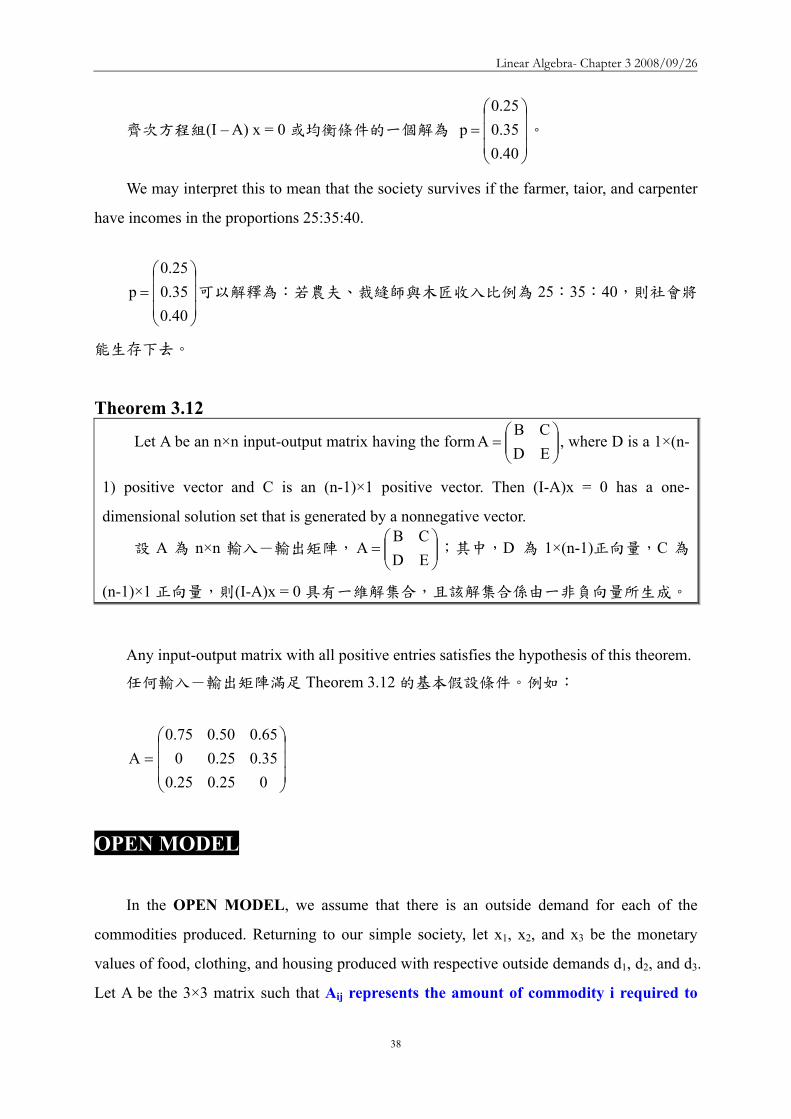
Linear Algebra- Chapter 3 20080926
38
齊次方程組(I ndash A) x = 0 或均衡條件的一個解為 ⎟⎟⎟
⎠
⎞
⎜⎜⎜
⎝
⎛=
400350250
p
We may interpret this to mean that the society survives if the farmer taior and carpenter
have incomes in the proportions 253540
⎟⎟⎟
⎠
⎞
⎜⎜⎜
⎝
⎛=
400350250
p 可以解釋為若農夫裁縫師與木匠收入比例為 253540則社會將
能生存下去
Theorem 312
Let A be an ntimesn input-output matrix having the form ⎟⎟⎠
⎞⎜⎜⎝
⎛=
EDCB
A where D is a 1times(n-
1) positive vector and C is an (n-1)times1 positive vector Then (I-A)x = 0 has a one-
dimensional solution set that is generated by a nonnegative vector
設 A 為 ntimesn 輸入-輸出矩陣 ⎟⎟⎠
⎞⎜⎜⎝
⎛=
EDCB
A 其中D 為 1times(n-1)正向量C 為
(n-1)times1 正向量則(I-A)x = 0 具有一維解集合且該解集合係由一非負向量所生成
Any input-output matrix with all positive entries satisfies the hypothesis of this theorem
任何輸入-輸出矩陣滿足 Theorem 312 的基本假設條件例如
⎟⎟⎟
⎠
⎞
⎜⎜⎜
⎝
⎛=
02502503502500650500750
A
OPEN MODEL
In the OPEN MODEL we assume that there is an outside demand for each of the
commodities produced Returning to our simple society let x1 x2 and x3 be the monetary
values of food clothing and housing produced with respective outside demands d1 d2 and d3
Let A be the 3times3 matrix such that Aij represents the amount of commodity i required to
Linear Algebra- Chapter 3 20080926
39
produce one monetary unit of commodity j Then the value of the surplus of food in the
society is x1 ndash (A11x1+A12x2+A13x3) that is the value of food produced minus the value of
food consumed while producing the three commodities The assumption that everything
produced is consumed gives us a similar equilibrium condition for the open model namely
that the surplus of each of the three commodities must equal the corresponding outside
demands Hence i
3
1jjiji dxAx =minussum
=
for j=1 2 3
在「開放模式」中我們假設每一產品皆有外來的需求在前述的單純社會裡
令 x1x2 與 x3 分別代表食物衣物與住屋的貨幣價值d1d2 與 d3 為食物衣物與住
屋的外來需求價值令 A 為 3times3 矩陣Aij 表示生產『一個貨幣單位』的產品 j 所需要
的產品 i 的價值於是此社會中食物的盈餘價值為 x1 ndash (A11x1+A12x2+A13x3)即食物的
價值減去生產食物衣物與住屋所需消耗的食物的價值意即生產出來的食物價值扣
掉用去生產食物衣物與住屋所消耗掉的價值)(A11A12A13 為生產一個貨幣單位
的食物 1衣物 2 與住屋 3 所需消耗的食物 1 數量A12x2 表示生產貨幣價值為 x2的衣物
所需要的食物價值)對每一種產品而言其盈餘價值等於外來的需求價值於是
i
3
1jjiji dxAx =minussum
=
for j=123
Suppose that 30 cents worth of food 10 cents worth of clothing and 30 cents worth of
housing are required for the production of $1 worth of food Similar suppose that 20 cents
worth of food 40 cents worth of clothing and 20 cents worth of housing are required for the
production of $1 worth of clothing Finally suppose that 30 cents worth of food 10 cents
worth of clothing and 30 cents worth of housing are required for the production of $1 worth
of housing Then the input-output matrix is
⎟⎟⎟
⎠
⎞
⎜⎜⎜
⎝
⎛=
300200300100400100300200300
A
假設生產價值 1 元的食物需要價值 30 分的食物(A11 = 03)價值 10 分的衣物
(A21 = 01)及價值 30 分的住屋(A31 = 03)生產價值 1 元的衣物需要價值 20 分的
食物(A12 = 02)價值 40 分的衣物(A22 = 04)及價值 20 分的住屋(A32 = 02)生
Linear Algebra- Chapter 3 20080926
40
產價值 1 元的住屋需要價值 30 分的食物(A13 = 03)價值 10 分的衣物(A23 = 01)
及價值 30 分的住屋(A33 = 03)於是輸入輸出矩陣 A 為
⎟⎟⎟
⎠
⎞
⎜⎜⎜
⎝
⎛=
300200300100400100300200300
A
若食物的外來需求值為 300 億元衣物為 200 億元住屋值為 1 百億元則
⎟⎟⎟
⎠
⎞
⎜⎜⎜
⎝
⎛=
⎟⎟⎟
⎠
⎞
⎜⎜⎜
⎝
⎛
⎟⎟⎟
⎠
⎞
⎜⎜⎜
⎝
⎛
minusminusminusminusminusminus
=minus=
minus
minus
700600900
100200300
700200300100600100300200300
d)AI(x
1
1
⎟⎟⎟
⎠
⎞
⎜⎜⎜
⎝
⎛=
700600900
x 表示要滿足外來需求必須生產的食物價值為 900 億元衣物價值為
600 億元住屋價值為 700 億元
Theorem
Let AX = Y be a system of n linear equations in n variables If Andash1 exists the
solution is unique and is given by X = Andash1Y
【Proof】
Substitute X = Andash1Y into the matrix equation
AX = A(Andash1Y) = (AAndash1)Y = InY = Y
The solution is unique
Let X1 be any solution thus AX1 = Y Multiplying both sides of this equation by Andash1
gives
Andash1AX1= Andash1Y InX1 = Andash1Y X1 = Andash1Y
Linear Algebra- Chapter 3 20080926
41
Example Example 1212
2x5x3x3x5x3x21x2x x
321
321
321
minus=++minus=minusminus=minusminus
⎥⎥⎥
⎦
⎤
⎢⎢⎢
⎣
⎡
minus=
⎥⎥⎥
⎦
⎤
⎢⎢⎢
⎣
⎡
⎥⎥⎥
⎦
⎤
⎢⎢⎢
⎣
⎡
minusminusminusminusminus
231
xxx
531532211
3
2
1
Solve the system of equations
This system can be written in the following matrix form
⎥⎥⎥
⎦
⎤
⎢⎢⎢
⎣
⎡
minus⎥⎥⎥
⎦
⎤
⎢⎢⎢
⎣
⎡
minusminusminusminusminus
=
⎥⎥⎥
⎦
⎤
⎢⎢⎢
⎣
⎡minus
231
531532211
xxx 1
3
2
1
If the matrix of coefficients is invertible the unique solutionIf the matrix of coefficients is invertible the unique solution isis
Example Example 2222
1 2 1 issolution unique The 321 =minus== xxx
⎥⎥⎥
⎦
⎤
⎢⎢⎢
⎣
⎡minus=
⎥⎥⎥
⎦
⎤
⎢⎢⎢
⎣
⎡
minus⎥⎥⎥
⎦
⎤
⎢⎢⎢
⎣
⎡
minusminusminus=
⎥⎥⎥
⎦
⎤
⎢⎢⎢
⎣
⎡
121
231
123135110
xxx
3
2
1
⎥⎥⎥
⎦
⎤
⎢⎢⎢
⎣
⎡
minusminusminus=
⎥⎥⎥
⎦
⎤
⎢⎢⎢
⎣
⎡
minusminusminusminusminus
=
minus
minus
123135110
531532211
A
1
1
The The LeontiefLeontief IO Model in IO Model in Economics Economics 1515
The Leontief input-output model is used to analyze the interdependence of economics Wassily Leontief received a Nobel Prize in 1973 for his work in thie fieldThe practical applications of this model have proliferated until it has now become a standard tool for investigating economic structures ranging from cities and corporation to states and countriesConsider an economics situation that involves ninterdependent industries The output of any one industry is needed as input by other industries and even possibly by the industry itself
The The LeontiefLeontief IO Model in IO Model in Economics Economics 2525
How a mathematical model involving a system of linear equations can be constructed to analyze such a situationAssume that each industry produces one commodity Let aij denote the amount of input of a certain commodity i to produce unit output of commodity j In our model let the amounts of input and output be measured in dollars Thus for example a34 = 045 means that 45 centsrsquo worth of commodity 3 is required to produce one dollarrsquos worth of commodity 4
The The LeontiefLeontief IO Model in IO Model in Economics Economics 3535
aij = amount of commodity i in one dollar of commodity jaij =生產一元價值的j產品需要耗用的i產品價值
The elements aij called input coefficients define a matrix A called the input-output matrix which describes the interdependence of the industriesExtending the model to include an open sector (all non-producing sectors) The product of industries may go not only into other producing industries but also into other non-producing sectors of the economy such as consumers and governments
The The LeontiefLeontief IO Model in IO Model in Economics Economics 4545
di = demand of the open sectors from industry ixi=total output of industry I necessary to meet demands of all n industries and the open sector
sectoropen of demand
nindustry of demand
2industry of demand
22
1industry of demand
11
industry ofoutput total
ininii
i
i dxaxaxax ++sdotsdotsdot++=
output ofportion sectoropen
output ofportion tryinterindusoutput total
DAXX +=Demand matrixDemand matrix
Output matrixOutput matrix
The The LeontiefLeontief IO Model in IO Model in Economics Economics 5555
Applying the model to the economy of a country X Applying the model to the economy of a country X represents the total output of each of the producing sectors represents the total output of each of the producing sectors of the economy and AX describes the contributions made of the economy and AX describes the contributions made by the various sectors to fulfilling the intersectional input by the various sectors to fulfilling the intersectional input requirements of the economyrequirements of the economyD is equal to (XD is equal to (X--AX) the difference between total output AX) the difference between total output X and industry transaction AXX and industry transaction AXD is thus the gross national product of the economyD is thus the gross national product of the economy
Example Example 1414
Consider an economy consisting of three industries having Consider an economy consisting of three industries having the following inputthe following input--output matrix output matrix AA Determine the output Determine the output levels required of the industries to meet the demands of levels required of the industries to meet the demands of the other industries and of the open sector in each casethe other industries and of the open sector in each case
in turn 321812
and 896
1612
9
5100
021
21
103
51
51
⎥⎥⎦
⎤
⎢⎢⎣
⎡
⎥⎥⎦
⎤
⎢⎢⎣
⎡
⎥⎥⎦
⎤
⎢⎢⎣
⎡=
⎥⎥⎥
⎦
⎤
⎢⎢⎢
⎣
⎡
= DA
The unit of The unit of DD are millions of dollarsare millions of dollars
Linear Algebra- Chapter 3 20080926
42
Example Example 2424
We wish to compute the output levels X that correspond to We wish to compute the output levels X that correspond to the various open sector demands D X is given by the the various open sector demands D X is given by the equation X = AX + D Rewritten as followsequation X = AX + D Rewritten as follows
X ndash AX = D rArr (I ndash A)X = D rArr X = (I ndash A) ndash1 D
⎥⎥⎥
⎦
⎤
⎢⎢⎢
⎣
⎡
=⎥⎥⎥
⎦
⎤
⎢⎢⎢
⎣
⎡
minus⎥⎥⎦
⎤
⎢⎢⎣
⎡=minus minus
minusminus
5400
021
21
103
51
54
5100
021
21
103
51
31
100010001
get We AI
⎥⎥⎥
⎦
⎤
⎢⎢⎢
⎣
⎡
=minus minus
4500
038
35
85
32
35
1)( AI
output ofingcorrespond valuesvarious
4500
038
35
85
32
35
)(
401020883957522133
32816189121269
)(
1
1
DAI
DAIX
minus
minus
minusuarruarruarruarruarruarruarr
⎥⎥⎦
⎤
⎢⎢⎣
⎡=
⎥⎥⎦
⎤
⎢⎢⎣
⎡
⎥⎥⎥
⎦
⎤
⎢⎢⎢
⎣
⎡
=minus=
Example Example 3434
By using Gauss-Jordan elimination
dollars of milliond are units The
40
15674
and 106629
209946
are 321812
and 896
1612
9
⎥⎥⎥
⎦
⎤
⎢⎢⎢
⎣
⎡
⎥⎥⎥
⎦
⎤
⎢⎢⎢
⎣
⎡
⎥⎥⎥
⎦
⎤
⎢⎢⎢
⎣
⎡
⎥⎥⎥
⎦
⎤
⎢⎢⎢
⎣
⎡
⎥⎥⎥
⎦
⎤
⎢⎢⎢
⎣
⎡
⎥⎥⎥
⎦
⎤
⎢⎢⎢
⎣
⎡
Example Example 4444
The output levels necessary to meet the demandsThe output levels necessary to meet the demands
IAAAIAI m =++++minus ))(( 2 L
mAAAIAI ++++=minus minus L21)(
Computing (IComputing (I--A) A) --11
1m
m2m2
m2
AI)AAAI(A)AAAI(I
)AAAI)(AI(
+minus=++++minus++++=
++++minusLL
L
NOTE 0A 1m rarr+
Population Movement Population Movement 1313
In 2000 58 million of people live in cities and 142 million of In 2000 58 million of people live in cities and 142 million of people people live in the surrounding suburbs Represent this information by tlive in the surrounding suburbs Represent this information by the he matrix matrix
The probability of a person staying in the city was 096 Thus tThe probability of a person staying in the city was 096 Thus the he probability of moving to the suburbs was 004 probability of moving to the suburbs was 004 The probability of a person moving to the city was 001 the The probability of a person moving to the city was 001 the probability of remaining in suburbia was 099probability of remaining in suburbia was 099
suburbcity
990040010960
suburbcity (to))from(
⎥⎦
⎤⎢⎣
⎡=P
⎥⎦
⎤⎢⎣
⎡=
14258
X0
City population in 2001 = people who remained from 2000 + peopleCity population in 2001 = people who remained from 2000 + peoplewho moved in from the suburbs = ( 096 who moved in from the suburbs = ( 096 timestimes 58 ) + (001 58 ) + (001 timestimes 142 ) = 142 ) = 571 million571 millionSuburban population in 2001 = people who moved in from the city Suburban population in 2001 = people who moved in from the city + people who stayed from 2000 = ( 004 + people who stayed from 2000 = ( 004 timestimes 58 ) + (099 58 ) + (099 timestimes 142 ) = 142 ) = 1429 million1429 millionCan arrive at these numbers using matrix multiplicationCan arrive at these numbers using matrix multiplication
⎥⎦
⎤⎢⎣
⎡=⎥
⎦
⎤⎢⎣
⎡⎥⎦
⎤⎢⎣
⎡==
9142157
14258
990040010960
PXX 01
Population Movement Population Movement 2323
Population Movement Population Movement 3333
Assume that the population flow represented by the matrix P is unchanged over the years The population distribution X2 after 2 years is given by X2 = P X1 = P2 X0 In general
Pn is called the n-step transition matrix The (ij)th element of Pngives the probability of going from state j to state i in n stepsFor example
in
ni XPX =+
suburbcity
960150040850
P
suburbcity (to))from(
4
⎥⎦
⎤⎢⎣
⎡=
The probability of living in the city in The probability of living in the city in 2000 and being in the suburbs 4 years 2000 and being in the suburbs 4 years later is 015later is 015
Markov ChainsMarkov Chains
The probabilities in the above model depend only on the The probabilities in the above model depend only on the current state of a person whether the person is living in the current state of a person whether the person is living in the city or in suburbiacity or in suburbiaThis type of model in which the probability of going from This type of model in which the probability of going from one state to another depends only on the current state one state to another depends only on the current state rather than on a more complete historical description is rather than on a more complete historical description is called a called a Markov chainMarkov chainMarkov chains are useful tools for scientists in many Markov chains are useful tools for scientists in many fields such as geneticsfields such as genetics
Linear Algebra- Chapter 3 20080926
43
GeneticsGenetics 1414
Genetics is the branch of biology that deals with Genetics is the branch of biology that deals with heredity heredity (遺傳)(遺傳) It is the study of units called It is the study of units called genes which determine the characteristics living genes which determine the characteristics living things inherit from their parents The inheritance things inherit from their parents The inheritance (遺傳)(遺傳)of such traitsof such traits(特徵)(特徵)as sex height eye as sex height eye color and hair color of human beings and such color and hair color of human beings and such traits as petaltraits as petal(花瓣)(花瓣) color and leaf shape of color and leaf shape of plants are governed by genesplants are governed by genesIn medicine agricultureIn medicine agriculturehelliphellip
GeneticsGenetics 2424
The traits of guinea pigsThe traits of guinea pigs(天竺鼠)(天竺鼠)are long hair and short hairare long hair and short hairThe length of hair is governed by a pair of gene which we denoteThe length of hair is governed by a pair of gene which we denote A A and aand aA guinea pig may have any one of the combination of AA A guinea pig may have any one of the combination of AA AaAa or or aaaa Each of these classes is called a genotypeEach of these classes is called a genotype(基因型)(基因型)The AA type guinea pig is indistinguishable in appearance from tThe AA type guinea pig is indistinguishable in appearance from the he AaAa type type ndashndash both have long hair both have long hair ndashndash whereas the whereas the aaaa type has short hairtype has short hairThe A gene is said to dominate the a geneThe A gene is said to dominate the a geneAn animal is called dominant An animal is called dominant (顯性)(顯性)if it has AA genes hybridif it has AA genes hybrid(混種)(混種) with with AaAa genes and recessive genes and recessive (隱性)(隱性)with with aaaa genesgenes
GeneticsGenetics 3434
When two guinea pigs are crossed the offspring inherits one genWhen two guinea pigs are crossed the offspring inherits one gene e from each parent in random mannerfrom each parent in random mannerGiven the genotype of the parents we can determine the Given the genotype of the parents we can determine the probabilities of the genotype of the offspringprobabilities of the genotype of the offspring
AA+AA AA+AA probabilities of AA probabilities of AA AaAa and and aaaa are 10and 0are 10and 0Aa+AAAa+AA probabilities of AA probabilities of AA AaAa and and aaaa are are frac12frac12 frac12frac12 and 0 and 0aa+AAaa+AA probabilities of AA probabilities of AA AaAa and and aaaa are 0 1 and 0are 0 1 and 0
This series of experiments is a Markov chain having transition This series of experiments is a Markov chain having transition matrixmatrix
aaAaAA
00012100211
P
aaAaAA
⎥⎥⎥
⎦
⎤
⎢⎢⎢
⎣
⎡=
GeneticsGenetics 4444
Assume an initial population of guinea pigs made up of an Assume an initial population of guinea pigs made up of an equal number of each genotypeequal number of each genotype
⎥⎥⎥
⎦
⎤
⎢⎢⎢
⎣
⎡=
313131
X0
The fractions of following generations are
⎥⎥⎥
⎦
⎤
⎢⎢⎢
⎣
⎡=
⎥⎥⎥
⎦
⎤
⎢⎢⎢
⎣
⎡=
⎥⎥⎥
⎦
⎤
⎢⎢⎢
⎣
⎡=
⎥⎥⎥
⎦
⎤
⎢⎢⎢
⎣
⎡=
01611615
X08187
X04143
X02121
X 4321
AAAAAaAaaaaa
3-4 Systems of Linear Equations ndash Computational Aspects
DEFINITION 36 Equivalent
Two systems of linear equations are called equivalent if they have the same solution
set
兩個線性方程組稱為等價意指兩者具有相同的解集合
Elementary Transformations Transformation called elementary transformations can be used to change a system of
linear equations into another system of linear equations that have the same solution
These transformations are used to solve system of linear equations by eliminating
variables
The equivalent transformations used in terms of matrix are called ELEMENTARY
ROW OPERATION
Linear Algebra- Chapter 3 20080926
44
Equivalent System Systems of equations that are related through elementary transformations are called
equivalent systems
Matrices that are related through elementary row operations are called row equivalent
matrices
The symbol asymp is used to indicate equivalence in both cases
Theorem 313 Let Ax = b be a system of m linear equations in n unknowns and let C be an invertible
mtimesm matrix Then the system (CA)x = Cb is equivalent to Ax = b
設 Ax = b 為含 n 個未知數m 個線性方程式的方程組若 C 為可逆的mtimesm
矩陣則(CA)x = Cb 等價於 Ax = b
【Proof】
Let K be the solution set for Ax = b and Krsquo the solution set for (CA)x = Cb If wisinK
then Aw = b So (CA)w = Cb and hence wisinKrsquo Thus KsubeKrsquo
Conversely if wisinKrsquo then (CA)w = Cb Hence Aw = C-1(CA)w = C-1(Cb) = b so
wisinK Thus KrsquosubeK and therefore K=Krsquo
設 K 為 Ax = b 的解集合且 Krsquo為(CA)x = Cb 的解集合
若 wisinK則 Aw = b (CA)w = Cb故 wisinKrsquo於是 KsubeKrsquo
反之若 wisinKrsquo則(CA)w = Cb Aw = C-1(CA)w = C-1(Cb) = b故 wisinK於是
KrsquosubeK因此K=Krsquo
Corollary Let Ax = b be a system of m linear equations in n unknowns If (Arsquo brsquo) is obtained ∣
from from (A b) by a finite number of elementary row operations then the system Arsquox = ∣
brsquo is equivalent to the original system
設 Ax = b 為含 n 個未知數m 個線性方程式的方程組若(Arsquo brsquo) ∣ 是由(A b) ∣
經過有限次數的基本列運算而得則 Arsquox = brsquo 等價於 Ax = b即兩者具有相同的解
集合
【Proof】
Suppose that (Arsquo brsquo) is obtained from (A b) by elementary row operations These ∣ ∣
Linear Algebra- Chapter 3 20080926
45
may be executed by multiplying (A b) by elementary mtimesm matrices E∣ 1 E2hellipEp Let
C=EphellipE2E1 then (Arsquo brsquo) = C(A b) = (CA Cb)∣ ∣ ∣
Since each Ei is invertible so is C Now Arsquo = CA and brsquo = Cb Thus by Theorem 313
the system Arsquox = brsquo is equivalent to the system Ax = b
設(Arsquo brsquo)∣ 是由(A b)∣ 經過基本列運算取得即以基本 mtimesm 矩陣 E1 E2hellipEp
乘上 (A b)∣ (Arsquo brsquo) = C(A b) = (CA Cb∣ ∣ ∣ )其中C=EphellipE2E1
因 Ei 可逆故 C 亦為可逆 Arsquo = CA 且 brsquo = Cb
依據 Theorem 313Arsquox = brsquo 等價於 Ax = b
Theorem 313 Let Ax = b be a system of m linear equations in n unknowns and let C be an
invertible mtimesm matrix Then the system (CA)x = Cb is equivalent to Ax = b 設 Ax = b
為含 n 個未知數m 個線性方程式的方程組若 C 為可逆的mtimesm 矩陣則(CA)x
= Cb 等價於 Ax = b
We now describe a method for solving any stystem of linear equations Consider for
example the system of linear equations
探討解線性方程組的方法hellip
2xxx2x3xxx1x2x3x2x3
4321
321
4321
=minus++=++=minus++
First we form the augmented matrix ⎟⎟⎟
⎠
⎞
⎜⎜⎜
⎝
⎛
minus
minus
231
112101112323
(增廣矩陣)
Interchanging the first and third rows ⎟⎟⎟
⎠
⎞
⎜⎜⎜
⎝
⎛
minus
minus
132
132301111121
(第 13 列互調)
Adding -1 times the first row to the second row and then add -3 times the first row to
the third row ⎟⎟⎟
⎠
⎞
⎜⎜⎜
⎝
⎛
minusminusminus
minus
512
104010101121
(第 1 列乘上 -1 加到第 2 列再以 -3 乘上
第 1 列加到第 3 列)
Linear Algebra- Chapter 3 20080926
46
Multiplying the second row by -1 ⎟⎟⎟
⎠
⎞
⎜⎜⎜
⎝
⎛
minusminus
minusminusminus
51
2
104010101121
(第 2 列乘上 -1)
Adding four times the second row to the third row ⎟⎟⎟
⎠
⎞
⎜⎜⎜
⎝
⎛
minusminus
minusminusminus
91
2
300010101121
(4 乘上第 2
列加到第 3 列)
Multiplying the third row by -13 ⎟⎟⎟
⎠
⎞
⎜⎜⎜
⎝
⎛minusminus
minus
31
2
100010101121
(第 3 列乘上 -13)
Adding the third row to the first and second rows to obtain zeros in row 1 column 4
and row 2 column 4 ⎟⎟⎟
⎠
⎞
⎜⎜⎜
⎝
⎛
325
100000100121
(將第 3 列加到第 1 列及第 2 列)
Adding -2 times the second row to the first row in order to make the first row second
column entry become zero ⎟⎟⎟
⎠
⎞
⎜⎜⎜
⎝
⎛
321
100000100101
(將第 2 列乘以 -2 再加至第 1 列)
We have now obtained the desired reduction of the augmented matrix
⎟⎟⎟
⎠
⎞
⎜⎜⎜
⎝
⎛
321
100000100101
是化簡後的增廣矩陣
This matrix corresponds to the system of linear equations
對應的線性方程組為
2x3x1xx
4
2
31
===+
By Corollary to Theorem 313 this system is equivalent to the original system But this
system is easily solved Obviously x2 = 2 and x4 = 3 Moreover x1 and x3 can be any values
Linear Algebra- Chapter 3 20080926
47
provided their sum is 1 Letting x3 = t we then have x1 = 1 ndash t Thus an arbitray solution to the
original system has the form
依據 Corollary to Theorem 313 化簡後的方程組與原方程組等值此方程組的解為
x2 = 3x4 = 3x1 + x3 = 1於是原方程組的任意解可以寫成
⎟⎟⎟⎟⎟
⎠
⎞
⎜⎜⎜⎜⎜
⎝
⎛minus
+
⎟⎟⎟⎟⎟
⎠
⎞
⎜⎜⎜⎜⎜
⎝
⎛
=
⎟⎟⎟⎟⎟
⎠
⎞
⎜⎜⎜⎜⎜
⎝
⎛ minus
0101
t
3021
3t2
t1
Observe that
⎪⎪⎭
⎪⎪⎬
⎫
⎪⎪⎩
⎪⎪⎨
⎧
⎟⎟⎟⎟⎟
⎠
⎞
⎜⎜⎜⎜⎜
⎝
⎛minus
0101
is a basis for the homogeneous system of equations
corresponding to the given system
其中
⎪⎪⎭
⎪⎪⎬
⎫
⎪⎪⎩
⎪⎪⎨
⎧
⎟⎟⎟⎟⎟
⎠
⎞
⎜⎜⎜⎜⎜
⎝
⎛minus
0101
是齊次方程組解集合的一組基底
Gauss-Jordan Elimination
Let A be an n times n matrix
1 Adjoin the identity n times n matrix In to A to form the matrix [A In]
2 Compute the reduced echelon form of [A In]
(1) If the reduced echelon form is of the type [In B] then B is the inverse of A
(2) If the reduced echelon form is not of the type [In B] in that the first n times n
submatrix is not In then A has no inverse
An n times n matrix A is invertible if and only if its reduced echelon form is In
DEFINITION 37 Reduced Row Echelon Form
A matrix is said to be in reduced row echelon form if the following three conditions
are satisfied
Linear Algebra- Chapter 3 20080926
48
一個矩陣可以被稱為簡約列梯形式必須具備有下列三條件
(a) Any row containing a nonzero entry preceeds any row in which all the entries are
zero (if any)
含有非零元素的任一列排在全含零元素的任一列前面(儘可能)
(b) The first nonzero entry in each row in the only nonzero entry in its column
各列中第一個非零元素為其所在行中唯一的非零元素
(c) The first nonzero entry in each row is 1 and it occurs in a column to thr right of the
first nonzero entry in the preceeding row
各列中第一個非零元素為 1 且它出現在前一列中第一個非零元素的右邊某一
行中
Reduced Echelon Form A matrix is in reduced echelon form if
1 Any rows consisting entirely of zeros are grouped at the bottom of the matrix
2 The first nonzero element of each other row is 1 This element is called a leading 1
3 The leading 1 of each row after the first is positioned to the right of the leading 1 of
the previous row
4 All other elements in a column that contains a leading 1 are zero
Theorem 314 Gaussian Elimination Transformation Gaussian elimination transform any matrix into its reduced row echelon form
利用 Gaussian elimination 將矩陣轉換成簡約列梯形式
We now describe a method for solving a system in which the augmented matrix is in
reduced row echelon form To illustrate this procedure we consider the system
14x8x3x2x2x28x5x2xxx6x3xxxx17x9x4xx3x2
54321
54321
54321
54321
=minus+++=minus+++=minus+++=minus+++
Linear Algebra- Chapter 3 20080926
49
for which the augmented matrix is
⎟⎟⎟⎟⎟
⎠
⎞
⎜⎜⎜⎜⎜
⎝
⎛
minusminusminusminus
1486
17
83222521113111194132
(增廣矩陣)
Applying Gaussian elimination to the augmented matrix of the system produces the
following sequence of matrices
利用 Gaussian elimination method 處理增廣矩陣
⎟⎟⎟⎟⎟
⎠
⎞
⎜⎜⎜⎜⎜
⎝
⎛
minusminusminusminus
1486
17
83222521113111194132
⎟⎟⎟⎟⎟
⎠
⎞
⎜⎜⎜⎜⎜
⎝
⎛
minusminusminusminus
148
176
83222521119413231111
⎟⎟⎟⎟⎟
⎠
⎞
⎜⎜⎜⎜⎜
⎝
⎛
minusminus
minus
0213
0000021000
1011020201
The system of linear equations corresponding to thus last matrix is
對應最後矩陣的線性方程組 2x2x
1xxx3x2x2x
54
532
531
=minus=+minus=minus+
Assign x3 = t1 x5 = t2
2t22x2x1tt1xxx
3t2t23x2x2x
254
21532
21531
+=+=+minus=+minus=
++minus=++minus=
Thus an arbitray solution s is of the form
於是任意解 s 具有下列形式
s =
⎟⎟⎟⎟⎟⎟
⎠
⎞
⎜⎜⎜⎜⎜⎜
⎝
⎛minus
+
⎟⎟⎟⎟⎟⎟
⎠
⎞
⎜⎜⎜⎜⎜⎜
⎝
⎛minus
+
⎟⎟⎟⎟⎟⎟
⎠
⎞
⎜⎜⎜⎜⎜⎜
⎝
⎛
=
⎟⎟⎟⎟⎟⎟
⎠
⎞
⎜⎜⎜⎜⎜⎜
⎝
⎛
+
+minus++minus
=
⎟⎟⎟⎟⎟⎟
⎠
⎞
⎜⎜⎜⎜⎜⎜
⎝
⎛
1201
2
t
00112
t
02013
t2t2
t1tt
3t2t2
xxxxx
21
2
2
1
21
21
5
4
3
2
1
where t1t2isinR
Linear Algebra- Chapter 3 20080926
50
Notice that
⎪⎪⎪
⎭
⎪⎪⎪
⎬
⎫
⎪⎪⎪
⎩
⎪⎪⎪
⎨
⎧
⎟⎟⎟⎟⎟⎟
⎠
⎞
⎜⎜⎜⎜⎜⎜
⎝
⎛minus
⎟⎟⎟⎟⎟⎟
⎠
⎞
⎜⎜⎜⎜⎜⎜
⎝
⎛minus
1201
2
00112
is a basis for the solution set of the corresponding
homogeneous system of equation and
⎟⎟⎟⎟⎟⎟
⎠
⎞
⎜⎜⎜⎜⎜⎜
⎝
⎛
02013
is a particular solution to the original system
⎪⎪⎪
⎭
⎪⎪⎪
⎬
⎫
⎪⎪⎪
⎩
⎪⎪⎪
⎨
⎧
⎟⎟⎟⎟⎟⎟
⎠
⎞
⎜⎜⎜⎜⎜⎜
⎝
⎛minus
⎟⎟⎟⎟⎟⎟
⎠
⎞
⎜⎜⎜⎜⎜⎜
⎝
⎛minus
1201
2
00112
是齊次方程組解集合的一組基底
⎟⎟⎟⎟⎟⎟
⎠
⎞
⎜⎜⎜⎜⎜⎜
⎝
⎛
02013
是原方程組的特別解
EXAMPLE 1
The matrix ⎟⎟⎟
⎠
⎞
⎜⎜⎜
⎝
⎛
101010011
is not in reduced row echelon form
因為第一行含有第一個非零元素在第一列但第一行尚含有其他非零元素
The matrix ⎟⎟⎟
⎠
⎞
⎜⎜⎜
⎝
⎛
110010012010
is not in reduced row echelon form
因為第一列第一個非零元素不在第一列第一個非零元素的右邊
The matrix ⎟⎟⎠
⎞⎜⎜⎝
⎛010002
is not in reduced row echelon form
因為第一列的第一個非零元素不是 1
Linear Algebra- Chapter 3 20080926
51
Reduced Echelon FormReduced Echelon Form
⎥⎥⎥
⎦
⎤
⎢⎢⎢
⎣
⎡
910030107001
⎥⎥⎥
⎦
⎤
⎢⎢⎢
⎣
⎡
100001000041
⎥⎥⎥
⎦
⎤
⎢⎢⎢
⎣
⎡
000210801
Not in Reduced Echelon Form
⎥⎥⎥
⎦
⎤
⎢⎢⎢
⎣
⎡
310000004021
⎥⎥⎥
⎦
⎤
⎢⎢⎢
⎣
⎡
100000430003021
⎥⎥⎥⎥
⎦
⎤
⎢⎢⎢⎢
⎣
⎡
0000210030108071
In Reduced Echelon Form
Use GaussUse Gauss--Jordan elimination to Jordan elimination to find reduced echelon formfind reduced echelon form 1313
Step 1 Interchange rows if necessary to bring a nonzero Step 1 Interchange rows if necessary to bring a nonzero element to the top of the first nonzero column This nonzero element to the top of the first nonzero column This nonzero element is called a pivotelement is called a pivot
⎥⎥⎦
⎤
⎢⎢⎣
⎡
minusminus
minus
1211244129333
22200
⎥⎥⎥
⎦
⎤
⎢⎢⎢
⎣
⎡
minusminus
minus
harrasymp
121124422200
129333
R2R1
Use GaussUse Gauss--Jordan elimination to Jordan elimination to find reduced echelon formfind reduced echelon form 2323
Step 2 Create a 1 in the pivot location by multiplying the Step 2 Create a 1 in the pivot location by multiplying the pivot row by 1pivotpivot row by 1pivot
Step 3 Create zero elsewhere in the pivot column by adding Step 3 Create zero elsewhere in the pivot column by adding suitable multiples of the pivot row to all other rows of the suitable multiples of the pivot row to all other rows of the matrixmatrix
⎥⎥⎥
⎦
⎤
⎢⎢⎢
⎣
⎡
minusminusminus
minus
minus+asymp
412002220043111
4)R1(R3
⎥⎥⎦
⎤
⎢⎢⎣
⎡
minusminus
minus
⎟⎠⎞
⎜⎝⎛asymp
12112442220043111
R13
1
The matrix is the reduced echelon form of the given matrixThe matrix is the reduced echelon form of the given matrix
Use GaussUse Gauss--Jordan elimination to Jordan elimination to find reduced echelon formfind reduced echelon form 3333
Step 4 Cover the pivot row and all rows above it Repeat Steps Step 4 Cover the pivot row and all rows above it Repeat Steps 1 1 and 2 for the remaining and 2 for the remaining submatrixsubmatrix Repeat Step 3 for the whole Repeat Step 3 for the whole matrix Continue until the reduced echelon form is reachedmatrix Continue until the reduced echelon form is reached
⎥⎥⎥
⎦
⎤
⎢⎢⎢
⎣
⎡
minusminus
+minus+asymp
⎥⎥⎥
⎦
⎤
⎢⎢⎢
⎣
⎡
minusminus
minus++asymp
⎥⎥⎥
⎦
⎤
⎢⎢⎢
⎣
⎡
minusminusminus
minus
⎟⎠⎞
⎜⎝⎛
asymp
⎥⎥⎥
⎦
⎤
⎢⎢⎢
⎣
⎡
minusminusminus
minus
6100050100
170011
R3R22)R3(R1
610001110052011
R2)2(R3R2R1
412001110043111
R221
412002220043111
Theorem 315 Let Ax = b be a system of r nonzero equations is in n unknown Suppose that rank(A)
= rank (A b)∣ and that (A b)∣ is in reduced row echelon form Then
設 Ax = b 為含有 n 個未知數r 個非零方程式的方程組假設 rank(A) = rank
(A b)∣ 且 (A b)∣ 為簡約列梯形式於是
(a) rank(A) = r
(b) If the general solution obtained by the procedure above is of the form s = s0 + t1u1
+ t2u2 +hellip+ tn-run-r then u1 u2hellip un-r is a basis for the solution set of the
corresponding homogeneous system and s0 is a solution to the original system 由
前述方法所得的 General solution 具有下列形式
s = s0 + t1u1 + t2u2 +hellip+ tn-run-r
其中u1 u2hellip un-r為齊次方程組 Ax = 0 的解集合的一組基底且 s0 為原方
程組的一個解)
【Proof】
Since (A b)∣ is in reduced row echelon form (A b)∣ must have r nonzero rows
Clearly these rows are linearly independent by the definition of the reduced row echelon
Linear Algebra- Chapter 3 20080926
52
form and so rank (A b)∣ = r Thus rank(A) = r
Let K be the solution set for Ax = b and let KH be the solution set for Ax = 0 Setting
t1 = t2 =hellip= tn-r = 0 we see that s = s0isinK But by Theorem 39 K = s +KH Hence
KH = - s0+K = span(u1 u2hellip un-r )
Because rank(A) = r we have dim(KH) = n-r Thus since dim(KH) = n-r and KH is
generated by a set u1 u2hellip un-r containing at most n-r vectors that is a basis for KH
由於(A b)∣ 具有簡約列梯形式因此(A b)∣ 必定具有 r 個非零列由簡約列梯形
式的定義得知 r 個非零列為線性獨立故 rank (A b)∣ = rrank(A) = r
令 K 為 Ax = b 的解集合 KH 為 Ax = 0 的解集合
假設 t1 = t2 =hellip= tn-r = 0(u1 u2hellip un-r非 KH的基底)則 s = s0isinK
依據 Theorem 39K = s +KH KH = - s0+K = span(u1 u2hellip un-r )
因 rank(A) = r所以 dim(KH) = n - r 且 KH 是由u1 u2hellip un-r 所生成
故原假設「t1 = t2 =hellip= tn-r = 0」不成立
因此 KH含有最多 n - r 個向量且這些向量為 KH的基底
Theorem 39 Let K be the solution set of a system of linear equations Ax = b and let KH be
the solution set of the corresponding homogeneous system Ax = 0 Then for any solution s
to Ax = b K =s + KH = s+k kisinKH 設 K 為線性方程組 Ax = b 的解集合且 KH
為對應的齊次方程組的解集合則對 Ax = b 的任一個解 s 而言K =s + KH = s+k
kisinKH
ExampleExampleSolve the system of equationsSolve the system of equations
7537429333
321
321
321
=minusminus=+minus=+minus
xxxxxxxxx
⎥⎥⎦
⎤
⎢⎢⎣
⎡
++asymp
000012104301
R2R3R2R1 12
431243
32
31
32
31+minus=+minus=rArr=+
=+rArr xxxx
xxxx
The general solution to the system isThe general solution to the system is
parameter) a (callednumber real is where 1243
3
2
1
rrxrxrx
=+minus=+minus=
⎥⎥⎥
⎦
⎤
⎢⎢⎢
⎣
⎡
minusminusminus
minus
minus+minus+asymp
⎥⎥⎥
⎦
⎤
⎢⎢⎢
⎣
⎡
minusminusminusminus
asymp
⎥⎥⎥
⎦
⎤
⎢⎢⎢
⎣
⎡
minusminusminusminus
242012103111
1R)3(3R1R)2(2R
715374123111
715374129333
R131
ExampleExample
Solve the system of equationsSolve the system of equations446942
1423258101242
4321
4321
4321
=minus+minusminus=+minus+minus
=minus+minus
xxxxxxxxxxxx
⎪⎪
⎩
⎪⎪
⎨
⎧
===
minus=
rArr==minus=minus
rArr
1x6xrx
2r2x
1x6x
2x2x
4
3
2
1
4
3
21
⎥⎥⎥
⎦
⎤
⎢⎢⎢
⎣
⎡ minusminusasymp
⎥⎥⎥
⎦
⎤
⎢⎢⎢
⎣
⎡minus
minusminusasymp
⎥⎥⎥
⎦
⎤
⎢⎢⎢
⎣
⎡
minusminusminusminusminusasymp
⎥⎥⎥
⎦
⎤
⎢⎢⎢
⎣
⎡
minusminusminusminusminusasymp
⎥⎥⎥
⎦
⎤
⎢⎢⎢
⎣
⎡
minusminusminusminusminus
minusminusasymp
⎥⎥⎥
⎦
⎤
⎢⎢⎢
⎣
⎡
minusminusminusminusminus
minusminus
+
minus+
+
minus+
minus+
+
110006010020021
110005110011021
14430051100
295621
2R31
144300153300295621
446942142321295621
44694214232158101242
R3R2
1)R3(R1
3R2R3
6)R2(R1
2)R1(R3
R1R2R1
21
Linear Algebra- Chapter 3 20080926
53
ExampleExampleSolve the system of equationsSolve the system of equations
432636242232
54321
54321
54321
=+minus+minusminus=++minus+=++minus+
xxxxxxxxxxxxxxx
⎥⎥⎦
⎤
⎢⎢⎣
⎡ minusasymp
⎥⎥⎦
⎤
⎢⎢⎣
⎡
minusminusminusminusminus
+
minus+
642000210000213121
431121636242213121
R1R3
2)R1(R2
⎥⎥⎦
⎤
⎢⎢⎣
⎡ minusasympharr 210000
642000213121
R3R2 ( ) ⎥⎥⎦
⎤
⎢⎢⎣
⎡ minusasymp
210000321000213121
2R21
⎥⎥⎦
⎤
⎢⎢⎣
⎡ minusminusminusasympminus+ 210000
321000750121
3)R2(R1 ⎥⎥⎦
⎤
⎢⎢⎣
⎡minus
minusasymp
minus+
+
210000101000300121
2)R3(R2
5R3R1
2x1x
3xx2x
5
4
321
=minus=
++minus=rArr
2xs and r somefor 1x sx rx
3sr2x
5
432
1
=minus===
++minus=
ExampleExample
Solve the system of Solve the system of equationsequations 122
32452232
32
321
321
321
=+minus=minus+
=+minus=+minus
xxxxxxxxxxx
⎥⎥
⎦
⎤
⎢⎢
⎣
⎡asymp
minusminusminus
minus
harr1220210063303211
R3R2
( ) ⎥⎥
⎦
⎤
⎢⎢
⎣
⎡asymp
minusminusminus
minus
1220210021103211
R231
⎥⎥
⎦
⎤
⎢⎢
⎣
⎡asympminusminusminus
minus+
+
5400210021101101
2)R2(R4
R2R1 ⎥⎥
⎦
⎤
⎢⎢
⎣
⎡asymp
minusminus
minus+
+
minus+
13000210040103001
4)R3R(R4
R3R2
1)R3(R1
( ) ⎥⎥
⎦
⎤
⎢⎢
⎣
⎡asymp
minusminus
1000210040103001
R4131
The system has no solutionThe system has no solution
⎥⎥
⎦
⎤
⎢⎢
⎣
⎡asymp
⎥⎥
⎦
⎤
⎢⎢
⎣
⎡
minusminusminus
minus
minusminusminusminus
minus+
minus+
1220633021003211
1220312145223211
1)R1(R3
2)R1(R2
0x1+0x2+0x3=1
Curve FittingCurve Fitting
A set of data points A set of data points is given and it is is given and it is necessary to find a polynomial whose graph passes through the necessary to find a polynomial whose graph passes through the points points The points are often measurements in an experiment The points are often measurements in an experiment The xThe x--coordinates are called coordinates are called base pointsbase pointsIt can be shown that if the base points are all distinct then aIt can be shown that if the base points are all distinct then a unique unique polynomial of degree n polynomial of degree n ndashndash 1 (or less)1 (or less)
can be fitted to thecan be fitted to the pointspoints
) ( ) ( ) ( 2211 nn yxyxyx K
11
2210
minusminus
minusminus ++++= n
nn
n xaxaxaay K
The coefficients can be found by substituting the points The coefficients can be found by substituting the points into the polynomial equation and then solving a system into the polynomial equation and then solving a system of linear equationsof linear equations
ExampleExample
Determine the equation of the polynomial of degree 2 whose graphpasses through the points (1 6) (2 3) (3 2)
Let the polynomial be and substituting x = 1 y = 6 x = 2 y = 3 x = 3 y = 2 we have
Solving this system for a0 a1 and a2 using Gauss-Jordan elimination
⎥⎥⎥
⎦
⎤
⎢⎢⎢
⎣
⎡minus
minus
minus+minus+asymp
220033109201
1)R2(R31)R2(R1
2210 xaxaay ++=
2a9a3a3a4a2a6aaa
210
210
210
=++=++=++
⎥⎥⎥
⎦
⎤
⎢⎢⎢
⎣
⎡
minusminus
⎥⎥⎥
⎦
⎤
⎢⎢⎢
⎣
⎡
minus+minus+asymp
482033106111
293134216111
1)R1(R31)R1(R2
( )⎥⎥⎥
⎦
⎤
⎢⎢⎢
⎣
⎡minus
⎥⎥⎥
⎦
⎤
⎢⎢⎢
⎣
⎡minus
minusasymp
minus++asymp
11006010
11001
110033109201
3)R3(R22R3R1
R321
We get a0 = 11 a1 = ndash 6 a2 = 1The parabola that passes through these points is y = 11 ndash 6x + x2
ExampleExample Traffic FlowTraffic Flow
Network analysis plays an important role in electrical Network analysis plays an important role in electrical engineeringengineeringThe concepts and tools of network analysis have been The concepts and tools of network analysis have been found to be useful in many other fields such as found to be useful in many other fields such as information theory and the study of transportation systemsinformation theory and the study of transportation systemsThe analysis of traffic flow through a road network during The analysis of traffic flow through a road network during peak period illustrates how systems of linear equations peak period illustrates how systems of linear equations with with manymany solutions can arise in practicesolutions can arise in practice
Traffic FlowTraffic Flow
Consider the typical road network The streets are all oneConsider the typical road network The streets are all one--way with the arrows indicating the direction of traffic flowway with the arrows indicating the direction of traffic flowThe flow of traffic in and out of the network is measured The flow of traffic in and out of the network is measured in vehicles per hour (in vehicles per hour (vphvph))How to construct a mathematical model to analyze this How to construct a mathematical model to analyze this network network
Traffic Traffic FlowFlowTRAFFIC LAWTRAFFIC LAWhelliphellipAll traffic entering an intersection must leave that All traffic entering an intersection must leave that intersectionintersection
Linear Algebra- Chapter 3 20080926
54
Junction AJunction BJunction CJunction DJunction EJunction F 600
800 200 500 100 600
54
643
73
72
621
51
=+=++minus=+minus=minus=+minus=+
xxxxx
xxxx
xxxxx
⎥⎥⎥⎥⎥⎥⎥⎥⎥⎥⎥⎥⎥
⎦
⎤
⎢⎢⎢⎢⎢⎢⎢⎢⎢⎢⎢⎢⎢
⎣
⎡
asympasymp
⎥⎥⎥⎥⎥⎥⎥⎥⎥⎥⎥⎥⎥
⎦
⎤
⎢⎢⎢⎢⎢⎢⎢⎢⎢⎢⎢⎢⎢
⎣
⎡
minusminus
minusminusminusminus
minusminus
minusminus
0000000001110000
6001101000200100010050010000106001100001
600001100080001011002001000100500100001010001000116000010001
L
Traffic FlowTraffic FlowJunction AJunction BJunction CJunction DJunction EJunction F 600
800 200 500 100 600
54
643
73
72
621
51
=+=++minus=+minus=minus=+minus=+
xxxxx
xxxx
xxxxx
Perform road work on x7 Because x3 ge 0 the minimum flow 200 in the branch x7 can be obtained by making x3 = 0 (closing DE to traffic)
Traffic FlowTraffic Flow
We get
765
76473
72761
xx x600xxx200x x500x x600xxx
minus=++minus=minus=+=+minusminus=
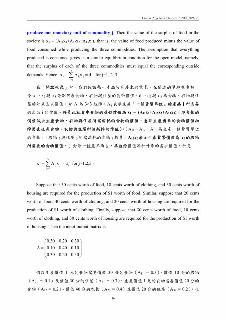
Linear Algebra- Chapter 3 20080926
39
produce one monetary unit of commodity j Then the value of the surplus of food in the
society is x1 ndash (A11x1+A12x2+A13x3) that is the value of food produced minus the value of
food consumed while producing the three commodities The assumption that everything
produced is consumed gives us a similar equilibrium condition for the open model namely
that the surplus of each of the three commodities must equal the corresponding outside
demands Hence i
3
1jjiji dxAx =minussum
=
for j=1 2 3
在「開放模式」中我們假設每一產品皆有外來的需求在前述的單純社會裡
令 x1x2 與 x3 分別代表食物衣物與住屋的貨幣價值d1d2 與 d3 為食物衣物與住
屋的外來需求價值令 A 為 3times3 矩陣Aij 表示生產『一個貨幣單位』的產品 j 所需要
的產品 i 的價值於是此社會中食物的盈餘價值為 x1 ndash (A11x1+A12x2+A13x3)即食物的
價值減去生產食物衣物與住屋所需消耗的食物的價值意即生產出來的食物價值扣
掉用去生產食物衣物與住屋所消耗掉的價值)(A11A12A13 為生產一個貨幣單位
的食物 1衣物 2 與住屋 3 所需消耗的食物 1 數量A12x2 表示生產貨幣價值為 x2的衣物
所需要的食物價值)對每一種產品而言其盈餘價值等於外來的需求價值於是
i
3
1jjiji dxAx =minussum
=
for j=123
Suppose that 30 cents worth of food 10 cents worth of clothing and 30 cents worth of
housing are required for the production of $1 worth of food Similar suppose that 20 cents
worth of food 40 cents worth of clothing and 20 cents worth of housing are required for the
production of $1 worth of clothing Finally suppose that 30 cents worth of food 10 cents
worth of clothing and 30 cents worth of housing are required for the production of $1 worth
of housing Then the input-output matrix is
⎟⎟⎟
⎠
⎞
⎜⎜⎜
⎝
⎛=
300200300100400100300200300
A
假設生產價值 1 元的食物需要價值 30 分的食物(A11 = 03)價值 10 分的衣物
(A21 = 01)及價值 30 分的住屋(A31 = 03)生產價值 1 元的衣物需要價值 20 分的
食物(A12 = 02)價值 40 分的衣物(A22 = 04)及價值 20 分的住屋(A32 = 02)生
Linear Algebra- Chapter 3 20080926
40
產價值 1 元的住屋需要價值 30 分的食物(A13 = 03)價值 10 分的衣物(A23 = 01)
及價值 30 分的住屋(A33 = 03)於是輸入輸出矩陣 A 為
⎟⎟⎟
⎠
⎞
⎜⎜⎜
⎝
⎛=
300200300100400100300200300
A
若食物的外來需求值為 300 億元衣物為 200 億元住屋值為 1 百億元則
⎟⎟⎟
⎠
⎞
⎜⎜⎜
⎝
⎛=
⎟⎟⎟
⎠
⎞
⎜⎜⎜
⎝
⎛
⎟⎟⎟
⎠
⎞
⎜⎜⎜
⎝
⎛
minusminusminusminusminusminus
=minus=
minus
minus
700600900
100200300
700200300100600100300200300
d)AI(x
1
1
⎟⎟⎟
⎠
⎞
⎜⎜⎜
⎝
⎛=
700600900
x 表示要滿足外來需求必須生產的食物價值為 900 億元衣物價值為
600 億元住屋價值為 700 億元
Theorem
Let AX = Y be a system of n linear equations in n variables If Andash1 exists the
solution is unique and is given by X = Andash1Y
【Proof】
Substitute X = Andash1Y into the matrix equation
AX = A(Andash1Y) = (AAndash1)Y = InY = Y
The solution is unique
Let X1 be any solution thus AX1 = Y Multiplying both sides of this equation by Andash1
gives
Andash1AX1= Andash1Y InX1 = Andash1Y X1 = Andash1Y
Linear Algebra- Chapter 3 20080926
41
Example Example 1212
2x5x3x3x5x3x21x2x x
321
321
321
minus=++minus=minusminus=minusminus
⎥⎥⎥
⎦
⎤
⎢⎢⎢
⎣
⎡
minus=
⎥⎥⎥
⎦
⎤
⎢⎢⎢
⎣
⎡
⎥⎥⎥
⎦
⎤
⎢⎢⎢
⎣
⎡
minusminusminusminusminus
231
xxx
531532211
3
2
1
Solve the system of equations
This system can be written in the following matrix form
⎥⎥⎥
⎦
⎤
⎢⎢⎢
⎣
⎡
minus⎥⎥⎥
⎦
⎤
⎢⎢⎢
⎣
⎡
minusminusminusminusminus
=
⎥⎥⎥
⎦
⎤
⎢⎢⎢
⎣
⎡minus
231
531532211
xxx 1
3
2
1
If the matrix of coefficients is invertible the unique solutionIf the matrix of coefficients is invertible the unique solution isis
Example Example 2222
1 2 1 issolution unique The 321 =minus== xxx
⎥⎥⎥
⎦
⎤
⎢⎢⎢
⎣
⎡minus=
⎥⎥⎥
⎦
⎤
⎢⎢⎢
⎣
⎡
minus⎥⎥⎥
⎦
⎤
⎢⎢⎢
⎣
⎡
minusminusminus=
⎥⎥⎥
⎦
⎤
⎢⎢⎢
⎣
⎡
121
231
123135110
xxx
3
2
1
⎥⎥⎥
⎦
⎤
⎢⎢⎢
⎣
⎡
minusminusminus=
⎥⎥⎥
⎦
⎤
⎢⎢⎢
⎣
⎡
minusminusminusminusminus
=
minus
minus
123135110
531532211
A
1
1
The The LeontiefLeontief IO Model in IO Model in Economics Economics 1515
The Leontief input-output model is used to analyze the interdependence of economics Wassily Leontief received a Nobel Prize in 1973 for his work in thie fieldThe practical applications of this model have proliferated until it has now become a standard tool for investigating economic structures ranging from cities and corporation to states and countriesConsider an economics situation that involves ninterdependent industries The output of any one industry is needed as input by other industries and even possibly by the industry itself
The The LeontiefLeontief IO Model in IO Model in Economics Economics 2525
How a mathematical model involving a system of linear equations can be constructed to analyze such a situationAssume that each industry produces one commodity Let aij denote the amount of input of a certain commodity i to produce unit output of commodity j In our model let the amounts of input and output be measured in dollars Thus for example a34 = 045 means that 45 centsrsquo worth of commodity 3 is required to produce one dollarrsquos worth of commodity 4
The The LeontiefLeontief IO Model in IO Model in Economics Economics 3535
aij = amount of commodity i in one dollar of commodity jaij =生產一元價值的j產品需要耗用的i產品價值
The elements aij called input coefficients define a matrix A called the input-output matrix which describes the interdependence of the industriesExtending the model to include an open sector (all non-producing sectors) The product of industries may go not only into other producing industries but also into other non-producing sectors of the economy such as consumers and governments
The The LeontiefLeontief IO Model in IO Model in Economics Economics 4545
di = demand of the open sectors from industry ixi=total output of industry I necessary to meet demands of all n industries and the open sector
sectoropen of demand
nindustry of demand
2industry of demand
22
1industry of demand
11
industry ofoutput total
ininii
i
i dxaxaxax ++sdotsdotsdot++=
output ofportion sectoropen
output ofportion tryinterindusoutput total
DAXX +=Demand matrixDemand matrix
Output matrixOutput matrix
The The LeontiefLeontief IO Model in IO Model in Economics Economics 5555
Applying the model to the economy of a country X Applying the model to the economy of a country X represents the total output of each of the producing sectors represents the total output of each of the producing sectors of the economy and AX describes the contributions made of the economy and AX describes the contributions made by the various sectors to fulfilling the intersectional input by the various sectors to fulfilling the intersectional input requirements of the economyrequirements of the economyD is equal to (XD is equal to (X--AX) the difference between total output AX) the difference between total output X and industry transaction AXX and industry transaction AXD is thus the gross national product of the economyD is thus the gross national product of the economy
Example Example 1414
Consider an economy consisting of three industries having Consider an economy consisting of three industries having the following inputthe following input--output matrix output matrix AA Determine the output Determine the output levels required of the industries to meet the demands of levels required of the industries to meet the demands of the other industries and of the open sector in each casethe other industries and of the open sector in each case
in turn 321812
and 896
1612
9
5100
021
21
103
51
51
⎥⎥⎦
⎤
⎢⎢⎣
⎡
⎥⎥⎦
⎤
⎢⎢⎣
⎡
⎥⎥⎦
⎤
⎢⎢⎣
⎡=
⎥⎥⎥
⎦
⎤
⎢⎢⎢
⎣
⎡
= DA
The unit of The unit of DD are millions of dollarsare millions of dollars
Linear Algebra- Chapter 3 20080926
42
Example Example 2424
We wish to compute the output levels X that correspond to We wish to compute the output levels X that correspond to the various open sector demands D X is given by the the various open sector demands D X is given by the equation X = AX + D Rewritten as followsequation X = AX + D Rewritten as follows
X ndash AX = D rArr (I ndash A)X = D rArr X = (I ndash A) ndash1 D
⎥⎥⎥
⎦
⎤
⎢⎢⎢
⎣
⎡
=⎥⎥⎥
⎦
⎤
⎢⎢⎢
⎣
⎡
minus⎥⎥⎦
⎤
⎢⎢⎣
⎡=minus minus
minusminus
5400
021
21
103
51
54
5100
021
21
103
51
31
100010001
get We AI
⎥⎥⎥
⎦
⎤
⎢⎢⎢
⎣
⎡
=minus minus
4500
038
35
85
32
35
1)( AI
output ofingcorrespond valuesvarious
4500
038
35
85
32
35
)(
401020883957522133
32816189121269
)(
1
1
DAI
DAIX
minus
minus
minusuarruarruarruarruarruarruarr
⎥⎥⎦
⎤
⎢⎢⎣
⎡=
⎥⎥⎦
⎤
⎢⎢⎣
⎡
⎥⎥⎥
⎦
⎤
⎢⎢⎢
⎣
⎡
=minus=
Example Example 3434
By using Gauss-Jordan elimination
dollars of milliond are units The
40
15674
and 106629
209946
are 321812
and 896
1612
9
⎥⎥⎥
⎦
⎤
⎢⎢⎢
⎣
⎡
⎥⎥⎥
⎦
⎤
⎢⎢⎢
⎣
⎡
⎥⎥⎥
⎦
⎤
⎢⎢⎢
⎣
⎡
⎥⎥⎥
⎦
⎤
⎢⎢⎢
⎣
⎡
⎥⎥⎥
⎦
⎤
⎢⎢⎢
⎣
⎡
⎥⎥⎥
⎦
⎤
⎢⎢⎢
⎣
⎡
Example Example 4444
The output levels necessary to meet the demandsThe output levels necessary to meet the demands
IAAAIAI m =++++minus ))(( 2 L
mAAAIAI ++++=minus minus L21)(
Computing (IComputing (I--A) A) --11
1m
m2m2
m2
AI)AAAI(A)AAAI(I
)AAAI)(AI(
+minus=++++minus++++=
++++minusLL
L
NOTE 0A 1m rarr+
Population Movement Population Movement 1313
In 2000 58 million of people live in cities and 142 million of In 2000 58 million of people live in cities and 142 million of people people live in the surrounding suburbs Represent this information by tlive in the surrounding suburbs Represent this information by the he matrix matrix
The probability of a person staying in the city was 096 Thus tThe probability of a person staying in the city was 096 Thus the he probability of moving to the suburbs was 004 probability of moving to the suburbs was 004 The probability of a person moving to the city was 001 the The probability of a person moving to the city was 001 the probability of remaining in suburbia was 099probability of remaining in suburbia was 099
suburbcity
990040010960
suburbcity (to))from(
⎥⎦
⎤⎢⎣
⎡=P
⎥⎦
⎤⎢⎣
⎡=
14258
X0
City population in 2001 = people who remained from 2000 + peopleCity population in 2001 = people who remained from 2000 + peoplewho moved in from the suburbs = ( 096 who moved in from the suburbs = ( 096 timestimes 58 ) + (001 58 ) + (001 timestimes 142 ) = 142 ) = 571 million571 millionSuburban population in 2001 = people who moved in from the city Suburban population in 2001 = people who moved in from the city + people who stayed from 2000 = ( 004 + people who stayed from 2000 = ( 004 timestimes 58 ) + (099 58 ) + (099 timestimes 142 ) = 142 ) = 1429 million1429 millionCan arrive at these numbers using matrix multiplicationCan arrive at these numbers using matrix multiplication
⎥⎦
⎤⎢⎣
⎡=⎥
⎦
⎤⎢⎣
⎡⎥⎦
⎤⎢⎣
⎡==
9142157
14258
990040010960
PXX 01
Population Movement Population Movement 2323
Population Movement Population Movement 3333
Assume that the population flow represented by the matrix P is unchanged over the years The population distribution X2 after 2 years is given by X2 = P X1 = P2 X0 In general
Pn is called the n-step transition matrix The (ij)th element of Pngives the probability of going from state j to state i in n stepsFor example
in
ni XPX =+
suburbcity
960150040850
P
suburbcity (to))from(
4
⎥⎦
⎤⎢⎣
⎡=
The probability of living in the city in The probability of living in the city in 2000 and being in the suburbs 4 years 2000 and being in the suburbs 4 years later is 015later is 015
Markov ChainsMarkov Chains
The probabilities in the above model depend only on the The probabilities in the above model depend only on the current state of a person whether the person is living in the current state of a person whether the person is living in the city or in suburbiacity or in suburbiaThis type of model in which the probability of going from This type of model in which the probability of going from one state to another depends only on the current state one state to another depends only on the current state rather than on a more complete historical description is rather than on a more complete historical description is called a called a Markov chainMarkov chainMarkov chains are useful tools for scientists in many Markov chains are useful tools for scientists in many fields such as geneticsfields such as genetics
Linear Algebra- Chapter 3 20080926
43
GeneticsGenetics 1414
Genetics is the branch of biology that deals with Genetics is the branch of biology that deals with heredity heredity (遺傳)(遺傳) It is the study of units called It is the study of units called genes which determine the characteristics living genes which determine the characteristics living things inherit from their parents The inheritance things inherit from their parents The inheritance (遺傳)(遺傳)of such traitsof such traits(特徵)(特徵)as sex height eye as sex height eye color and hair color of human beings and such color and hair color of human beings and such traits as petaltraits as petal(花瓣)(花瓣) color and leaf shape of color and leaf shape of plants are governed by genesplants are governed by genesIn medicine agricultureIn medicine agriculturehelliphellip
GeneticsGenetics 2424
The traits of guinea pigsThe traits of guinea pigs(天竺鼠)(天竺鼠)are long hair and short hairare long hair and short hairThe length of hair is governed by a pair of gene which we denoteThe length of hair is governed by a pair of gene which we denote A A and aand aA guinea pig may have any one of the combination of AA A guinea pig may have any one of the combination of AA AaAa or or aaaa Each of these classes is called a genotypeEach of these classes is called a genotype(基因型)(基因型)The AA type guinea pig is indistinguishable in appearance from tThe AA type guinea pig is indistinguishable in appearance from the he AaAa type type ndashndash both have long hair both have long hair ndashndash whereas the whereas the aaaa type has short hairtype has short hairThe A gene is said to dominate the a geneThe A gene is said to dominate the a geneAn animal is called dominant An animal is called dominant (顯性)(顯性)if it has AA genes hybridif it has AA genes hybrid(混種)(混種) with with AaAa genes and recessive genes and recessive (隱性)(隱性)with with aaaa genesgenes
GeneticsGenetics 3434
When two guinea pigs are crossed the offspring inherits one genWhen two guinea pigs are crossed the offspring inherits one gene e from each parent in random mannerfrom each parent in random mannerGiven the genotype of the parents we can determine the Given the genotype of the parents we can determine the probabilities of the genotype of the offspringprobabilities of the genotype of the offspring
AA+AA AA+AA probabilities of AA probabilities of AA AaAa and and aaaa are 10and 0are 10and 0Aa+AAAa+AA probabilities of AA probabilities of AA AaAa and and aaaa are are frac12frac12 frac12frac12 and 0 and 0aa+AAaa+AA probabilities of AA probabilities of AA AaAa and and aaaa are 0 1 and 0are 0 1 and 0
This series of experiments is a Markov chain having transition This series of experiments is a Markov chain having transition matrixmatrix
aaAaAA
00012100211
P
aaAaAA
⎥⎥⎥
⎦
⎤
⎢⎢⎢
⎣
⎡=
GeneticsGenetics 4444
Assume an initial population of guinea pigs made up of an Assume an initial population of guinea pigs made up of an equal number of each genotypeequal number of each genotype
⎥⎥⎥
⎦
⎤
⎢⎢⎢
⎣
⎡=
313131
X0
The fractions of following generations are
⎥⎥⎥
⎦
⎤
⎢⎢⎢
⎣
⎡=
⎥⎥⎥
⎦
⎤
⎢⎢⎢
⎣
⎡=
⎥⎥⎥
⎦
⎤
⎢⎢⎢
⎣
⎡=
⎥⎥⎥
⎦
⎤
⎢⎢⎢
⎣
⎡=
01611615
X08187
X04143
X02121
X 4321
AAAAAaAaaaaa
3-4 Systems of Linear Equations ndash Computational Aspects
DEFINITION 36 Equivalent
Two systems of linear equations are called equivalent if they have the same solution
set
兩個線性方程組稱為等價意指兩者具有相同的解集合
Elementary Transformations Transformation called elementary transformations can be used to change a system of
linear equations into another system of linear equations that have the same solution
These transformations are used to solve system of linear equations by eliminating
variables
The equivalent transformations used in terms of matrix are called ELEMENTARY
ROW OPERATION
Linear Algebra- Chapter 3 20080926
44
Equivalent System Systems of equations that are related through elementary transformations are called
equivalent systems
Matrices that are related through elementary row operations are called row equivalent
matrices
The symbol asymp is used to indicate equivalence in both cases
Theorem 313 Let Ax = b be a system of m linear equations in n unknowns and let C be an invertible
mtimesm matrix Then the system (CA)x = Cb is equivalent to Ax = b
設 Ax = b 為含 n 個未知數m 個線性方程式的方程組若 C 為可逆的mtimesm
矩陣則(CA)x = Cb 等價於 Ax = b
【Proof】
Let K be the solution set for Ax = b and Krsquo the solution set for (CA)x = Cb If wisinK
then Aw = b So (CA)w = Cb and hence wisinKrsquo Thus KsubeKrsquo
Conversely if wisinKrsquo then (CA)w = Cb Hence Aw = C-1(CA)w = C-1(Cb) = b so
wisinK Thus KrsquosubeK and therefore K=Krsquo
設 K 為 Ax = b 的解集合且 Krsquo為(CA)x = Cb 的解集合
若 wisinK則 Aw = b (CA)w = Cb故 wisinKrsquo於是 KsubeKrsquo
反之若 wisinKrsquo則(CA)w = Cb Aw = C-1(CA)w = C-1(Cb) = b故 wisinK於是
KrsquosubeK因此K=Krsquo
Corollary Let Ax = b be a system of m linear equations in n unknowns If (Arsquo brsquo) is obtained ∣
from from (A b) by a finite number of elementary row operations then the system Arsquox = ∣
brsquo is equivalent to the original system
設 Ax = b 為含 n 個未知數m 個線性方程式的方程組若(Arsquo brsquo) ∣ 是由(A b) ∣
經過有限次數的基本列運算而得則 Arsquox = brsquo 等價於 Ax = b即兩者具有相同的解
集合
【Proof】
Suppose that (Arsquo brsquo) is obtained from (A b) by elementary row operations These ∣ ∣
Linear Algebra- Chapter 3 20080926
45
may be executed by multiplying (A b) by elementary mtimesm matrices E∣ 1 E2hellipEp Let
C=EphellipE2E1 then (Arsquo brsquo) = C(A b) = (CA Cb)∣ ∣ ∣
Since each Ei is invertible so is C Now Arsquo = CA and brsquo = Cb Thus by Theorem 313
the system Arsquox = brsquo is equivalent to the system Ax = b
設(Arsquo brsquo)∣ 是由(A b)∣ 經過基本列運算取得即以基本 mtimesm 矩陣 E1 E2hellipEp
乘上 (A b)∣ (Arsquo brsquo) = C(A b) = (CA Cb∣ ∣ ∣ )其中C=EphellipE2E1
因 Ei 可逆故 C 亦為可逆 Arsquo = CA 且 brsquo = Cb
依據 Theorem 313Arsquox = brsquo 等價於 Ax = b
Theorem 313 Let Ax = b be a system of m linear equations in n unknowns and let C be an
invertible mtimesm matrix Then the system (CA)x = Cb is equivalent to Ax = b 設 Ax = b
為含 n 個未知數m 個線性方程式的方程組若 C 為可逆的mtimesm 矩陣則(CA)x
= Cb 等價於 Ax = b
We now describe a method for solving any stystem of linear equations Consider for
example the system of linear equations
探討解線性方程組的方法hellip
2xxx2x3xxx1x2x3x2x3
4321
321
4321
=minus++=++=minus++
First we form the augmented matrix ⎟⎟⎟
⎠
⎞
⎜⎜⎜
⎝
⎛
minus
minus
231
112101112323
(增廣矩陣)
Interchanging the first and third rows ⎟⎟⎟
⎠
⎞
⎜⎜⎜
⎝
⎛
minus
minus
132
132301111121
(第 13 列互調)
Adding -1 times the first row to the second row and then add -3 times the first row to
the third row ⎟⎟⎟
⎠
⎞
⎜⎜⎜
⎝
⎛
minusminusminus
minus
512
104010101121
(第 1 列乘上 -1 加到第 2 列再以 -3 乘上
第 1 列加到第 3 列)
Linear Algebra- Chapter 3 20080926
46
Multiplying the second row by -1 ⎟⎟⎟
⎠
⎞
⎜⎜⎜
⎝
⎛
minusminus
minusminusminus
51
2
104010101121
(第 2 列乘上 -1)
Adding four times the second row to the third row ⎟⎟⎟
⎠
⎞
⎜⎜⎜
⎝
⎛
minusminus
minusminusminus
91
2
300010101121
(4 乘上第 2
列加到第 3 列)
Multiplying the third row by -13 ⎟⎟⎟
⎠
⎞
⎜⎜⎜
⎝
⎛minusminus
minus
31
2
100010101121
(第 3 列乘上 -13)
Adding the third row to the first and second rows to obtain zeros in row 1 column 4
and row 2 column 4 ⎟⎟⎟
⎠
⎞
⎜⎜⎜
⎝
⎛
325
100000100121
(將第 3 列加到第 1 列及第 2 列)
Adding -2 times the second row to the first row in order to make the first row second
column entry become zero ⎟⎟⎟
⎠
⎞
⎜⎜⎜
⎝
⎛
321
100000100101
(將第 2 列乘以 -2 再加至第 1 列)
We have now obtained the desired reduction of the augmented matrix
⎟⎟⎟
⎠
⎞
⎜⎜⎜
⎝
⎛
321
100000100101
是化簡後的增廣矩陣
This matrix corresponds to the system of linear equations
對應的線性方程組為
2x3x1xx
4
2
31
===+
By Corollary to Theorem 313 this system is equivalent to the original system But this
system is easily solved Obviously x2 = 2 and x4 = 3 Moreover x1 and x3 can be any values
Linear Algebra- Chapter 3 20080926
47
provided their sum is 1 Letting x3 = t we then have x1 = 1 ndash t Thus an arbitray solution to the
original system has the form
依據 Corollary to Theorem 313 化簡後的方程組與原方程組等值此方程組的解為
x2 = 3x4 = 3x1 + x3 = 1於是原方程組的任意解可以寫成
⎟⎟⎟⎟⎟
⎠
⎞
⎜⎜⎜⎜⎜
⎝
⎛minus
+
⎟⎟⎟⎟⎟
⎠
⎞
⎜⎜⎜⎜⎜
⎝
⎛
=
⎟⎟⎟⎟⎟
⎠
⎞
⎜⎜⎜⎜⎜
⎝
⎛ minus
0101
t
3021
3t2
t1
Observe that
⎪⎪⎭
⎪⎪⎬
⎫
⎪⎪⎩
⎪⎪⎨
⎧
⎟⎟⎟⎟⎟
⎠
⎞
⎜⎜⎜⎜⎜
⎝
⎛minus
0101
is a basis for the homogeneous system of equations
corresponding to the given system
其中
⎪⎪⎭
⎪⎪⎬
⎫
⎪⎪⎩
⎪⎪⎨
⎧
⎟⎟⎟⎟⎟
⎠
⎞
⎜⎜⎜⎜⎜
⎝
⎛minus
0101
是齊次方程組解集合的一組基底
Gauss-Jordan Elimination
Let A be an n times n matrix
1 Adjoin the identity n times n matrix In to A to form the matrix [A In]
2 Compute the reduced echelon form of [A In]
(1) If the reduced echelon form is of the type [In B] then B is the inverse of A
(2) If the reduced echelon form is not of the type [In B] in that the first n times n
submatrix is not In then A has no inverse
An n times n matrix A is invertible if and only if its reduced echelon form is In
DEFINITION 37 Reduced Row Echelon Form
A matrix is said to be in reduced row echelon form if the following three conditions
are satisfied
Linear Algebra- Chapter 3 20080926
48
一個矩陣可以被稱為簡約列梯形式必須具備有下列三條件
(a) Any row containing a nonzero entry preceeds any row in which all the entries are
zero (if any)
含有非零元素的任一列排在全含零元素的任一列前面(儘可能)
(b) The first nonzero entry in each row in the only nonzero entry in its column
各列中第一個非零元素為其所在行中唯一的非零元素
(c) The first nonzero entry in each row is 1 and it occurs in a column to thr right of the
first nonzero entry in the preceeding row
各列中第一個非零元素為 1 且它出現在前一列中第一個非零元素的右邊某一
行中
Reduced Echelon Form A matrix is in reduced echelon form if
1 Any rows consisting entirely of zeros are grouped at the bottom of the matrix
2 The first nonzero element of each other row is 1 This element is called a leading 1
3 The leading 1 of each row after the first is positioned to the right of the leading 1 of
the previous row
4 All other elements in a column that contains a leading 1 are zero
Theorem 314 Gaussian Elimination Transformation Gaussian elimination transform any matrix into its reduced row echelon form
利用 Gaussian elimination 將矩陣轉換成簡約列梯形式
We now describe a method for solving a system in which the augmented matrix is in
reduced row echelon form To illustrate this procedure we consider the system
14x8x3x2x2x28x5x2xxx6x3xxxx17x9x4xx3x2
54321
54321
54321
54321
=minus+++=minus+++=minus+++=minus+++
Linear Algebra- Chapter 3 20080926
49
for which the augmented matrix is
⎟⎟⎟⎟⎟
⎠
⎞
⎜⎜⎜⎜⎜
⎝
⎛
minusminusminusminus
1486
17
83222521113111194132
(增廣矩陣)
Applying Gaussian elimination to the augmented matrix of the system produces the
following sequence of matrices
利用 Gaussian elimination method 處理增廣矩陣
⎟⎟⎟⎟⎟
⎠
⎞
⎜⎜⎜⎜⎜
⎝
⎛
minusminusminusminus
1486
17
83222521113111194132
⎟⎟⎟⎟⎟
⎠
⎞
⎜⎜⎜⎜⎜
⎝
⎛
minusminusminusminus
148
176
83222521119413231111
⎟⎟⎟⎟⎟
⎠
⎞
⎜⎜⎜⎜⎜
⎝
⎛
minusminus
minus
0213
0000021000
1011020201
The system of linear equations corresponding to thus last matrix is
對應最後矩陣的線性方程組 2x2x
1xxx3x2x2x
54
532
531
=minus=+minus=minus+
Assign x3 = t1 x5 = t2
2t22x2x1tt1xxx
3t2t23x2x2x
254
21532
21531
+=+=+minus=+minus=
++minus=++minus=
Thus an arbitray solution s is of the form
於是任意解 s 具有下列形式
s =
⎟⎟⎟⎟⎟⎟
⎠
⎞
⎜⎜⎜⎜⎜⎜
⎝
⎛minus
+
⎟⎟⎟⎟⎟⎟
⎠
⎞
⎜⎜⎜⎜⎜⎜
⎝
⎛minus
+
⎟⎟⎟⎟⎟⎟
⎠
⎞
⎜⎜⎜⎜⎜⎜
⎝
⎛
=
⎟⎟⎟⎟⎟⎟
⎠
⎞
⎜⎜⎜⎜⎜⎜
⎝
⎛
+
+minus++minus
=
⎟⎟⎟⎟⎟⎟
⎠
⎞
⎜⎜⎜⎜⎜⎜
⎝
⎛
1201
2
t
00112
t
02013
t2t2
t1tt
3t2t2
xxxxx
21
2
2
1
21
21
5
4
3
2
1
where t1t2isinR
Linear Algebra- Chapter 3 20080926
50
Notice that
⎪⎪⎪
⎭
⎪⎪⎪
⎬
⎫
⎪⎪⎪
⎩
⎪⎪⎪
⎨
⎧
⎟⎟⎟⎟⎟⎟
⎠
⎞
⎜⎜⎜⎜⎜⎜
⎝
⎛minus
⎟⎟⎟⎟⎟⎟
⎠
⎞
⎜⎜⎜⎜⎜⎜
⎝
⎛minus
1201
2
00112
is a basis for the solution set of the corresponding
homogeneous system of equation and
⎟⎟⎟⎟⎟⎟
⎠
⎞
⎜⎜⎜⎜⎜⎜
⎝
⎛
02013
is a particular solution to the original system
⎪⎪⎪
⎭
⎪⎪⎪
⎬
⎫
⎪⎪⎪
⎩
⎪⎪⎪
⎨
⎧
⎟⎟⎟⎟⎟⎟
⎠
⎞
⎜⎜⎜⎜⎜⎜
⎝
⎛minus
⎟⎟⎟⎟⎟⎟
⎠
⎞
⎜⎜⎜⎜⎜⎜
⎝
⎛minus
1201
2
00112
是齊次方程組解集合的一組基底
⎟⎟⎟⎟⎟⎟
⎠
⎞
⎜⎜⎜⎜⎜⎜
⎝
⎛
02013
是原方程組的特別解
EXAMPLE 1
The matrix ⎟⎟⎟
⎠
⎞
⎜⎜⎜
⎝
⎛
101010011
is not in reduced row echelon form
因為第一行含有第一個非零元素在第一列但第一行尚含有其他非零元素
The matrix ⎟⎟⎟
⎠
⎞
⎜⎜⎜
⎝
⎛
110010012010
is not in reduced row echelon form
因為第一列第一個非零元素不在第一列第一個非零元素的右邊
The matrix ⎟⎟⎠
⎞⎜⎜⎝
⎛010002
is not in reduced row echelon form
因為第一列的第一個非零元素不是 1
Linear Algebra- Chapter 3 20080926
51
Reduced Echelon FormReduced Echelon Form
⎥⎥⎥
⎦
⎤
⎢⎢⎢
⎣
⎡
910030107001
⎥⎥⎥
⎦
⎤
⎢⎢⎢
⎣
⎡
100001000041
⎥⎥⎥
⎦
⎤
⎢⎢⎢
⎣
⎡
000210801
Not in Reduced Echelon Form
⎥⎥⎥
⎦
⎤
⎢⎢⎢
⎣
⎡
310000004021
⎥⎥⎥
⎦
⎤
⎢⎢⎢
⎣
⎡
100000430003021
⎥⎥⎥⎥
⎦
⎤
⎢⎢⎢⎢
⎣
⎡
0000210030108071
In Reduced Echelon Form
Use GaussUse Gauss--Jordan elimination to Jordan elimination to find reduced echelon formfind reduced echelon form 1313
Step 1 Interchange rows if necessary to bring a nonzero Step 1 Interchange rows if necessary to bring a nonzero element to the top of the first nonzero column This nonzero element to the top of the first nonzero column This nonzero element is called a pivotelement is called a pivot
⎥⎥⎦
⎤
⎢⎢⎣
⎡
minusminus
minus
1211244129333
22200
⎥⎥⎥
⎦
⎤
⎢⎢⎢
⎣
⎡
minusminus
minus
harrasymp
121124422200
129333
R2R1
Use GaussUse Gauss--Jordan elimination to Jordan elimination to find reduced echelon formfind reduced echelon form 2323
Step 2 Create a 1 in the pivot location by multiplying the Step 2 Create a 1 in the pivot location by multiplying the pivot row by 1pivotpivot row by 1pivot
Step 3 Create zero elsewhere in the pivot column by adding Step 3 Create zero elsewhere in the pivot column by adding suitable multiples of the pivot row to all other rows of the suitable multiples of the pivot row to all other rows of the matrixmatrix
⎥⎥⎥
⎦
⎤
⎢⎢⎢
⎣
⎡
minusminusminus
minus
minus+asymp
412002220043111
4)R1(R3
⎥⎥⎦
⎤
⎢⎢⎣
⎡
minusminus
minus
⎟⎠⎞
⎜⎝⎛asymp
12112442220043111
R13
1
The matrix is the reduced echelon form of the given matrixThe matrix is the reduced echelon form of the given matrix
Use GaussUse Gauss--Jordan elimination to Jordan elimination to find reduced echelon formfind reduced echelon form 3333
Step 4 Cover the pivot row and all rows above it Repeat Steps Step 4 Cover the pivot row and all rows above it Repeat Steps 1 1 and 2 for the remaining and 2 for the remaining submatrixsubmatrix Repeat Step 3 for the whole Repeat Step 3 for the whole matrix Continue until the reduced echelon form is reachedmatrix Continue until the reduced echelon form is reached
⎥⎥⎥
⎦
⎤
⎢⎢⎢
⎣
⎡
minusminus
+minus+asymp
⎥⎥⎥
⎦
⎤
⎢⎢⎢
⎣
⎡
minusminus
minus++asymp
⎥⎥⎥
⎦
⎤
⎢⎢⎢
⎣
⎡
minusminusminus
minus
⎟⎠⎞
⎜⎝⎛
asymp
⎥⎥⎥
⎦
⎤
⎢⎢⎢
⎣
⎡
minusminusminus
minus
6100050100
170011
R3R22)R3(R1
610001110052011
R2)2(R3R2R1
412001110043111
R221
412002220043111
Theorem 315 Let Ax = b be a system of r nonzero equations is in n unknown Suppose that rank(A)
= rank (A b)∣ and that (A b)∣ is in reduced row echelon form Then
設 Ax = b 為含有 n 個未知數r 個非零方程式的方程組假設 rank(A) = rank
(A b)∣ 且 (A b)∣ 為簡約列梯形式於是
(a) rank(A) = r
(b) If the general solution obtained by the procedure above is of the form s = s0 + t1u1
+ t2u2 +hellip+ tn-run-r then u1 u2hellip un-r is a basis for the solution set of the
corresponding homogeneous system and s0 is a solution to the original system 由
前述方法所得的 General solution 具有下列形式
s = s0 + t1u1 + t2u2 +hellip+ tn-run-r
其中u1 u2hellip un-r為齊次方程組 Ax = 0 的解集合的一組基底且 s0 為原方
程組的一個解)
【Proof】
Since (A b)∣ is in reduced row echelon form (A b)∣ must have r nonzero rows
Clearly these rows are linearly independent by the definition of the reduced row echelon
Linear Algebra- Chapter 3 20080926
52
form and so rank (A b)∣ = r Thus rank(A) = r
Let K be the solution set for Ax = b and let KH be the solution set for Ax = 0 Setting
t1 = t2 =hellip= tn-r = 0 we see that s = s0isinK But by Theorem 39 K = s +KH Hence
KH = - s0+K = span(u1 u2hellip un-r )
Because rank(A) = r we have dim(KH) = n-r Thus since dim(KH) = n-r and KH is
generated by a set u1 u2hellip un-r containing at most n-r vectors that is a basis for KH
由於(A b)∣ 具有簡約列梯形式因此(A b)∣ 必定具有 r 個非零列由簡約列梯形
式的定義得知 r 個非零列為線性獨立故 rank (A b)∣ = rrank(A) = r
令 K 為 Ax = b 的解集合 KH 為 Ax = 0 的解集合
假設 t1 = t2 =hellip= tn-r = 0(u1 u2hellip un-r非 KH的基底)則 s = s0isinK
依據 Theorem 39K = s +KH KH = - s0+K = span(u1 u2hellip un-r )
因 rank(A) = r所以 dim(KH) = n - r 且 KH 是由u1 u2hellip un-r 所生成
故原假設「t1 = t2 =hellip= tn-r = 0」不成立
因此 KH含有最多 n - r 個向量且這些向量為 KH的基底
Theorem 39 Let K be the solution set of a system of linear equations Ax = b and let KH be
the solution set of the corresponding homogeneous system Ax = 0 Then for any solution s
to Ax = b K =s + KH = s+k kisinKH 設 K 為線性方程組 Ax = b 的解集合且 KH
為對應的齊次方程組的解集合則對 Ax = b 的任一個解 s 而言K =s + KH = s+k
kisinKH
ExampleExampleSolve the system of equationsSolve the system of equations
7537429333
321
321
321
=minusminus=+minus=+minus
xxxxxxxxx
⎥⎥⎦
⎤
⎢⎢⎣
⎡
++asymp
000012104301
R2R3R2R1 12
431243
32
31
32
31+minus=+minus=rArr=+
=+rArr xxxx
xxxx
The general solution to the system isThe general solution to the system is
parameter) a (callednumber real is where 1243
3
2
1
rrxrxrx
=+minus=+minus=
⎥⎥⎥
⎦
⎤
⎢⎢⎢
⎣
⎡
minusminusminus
minus
minus+minus+asymp
⎥⎥⎥
⎦
⎤
⎢⎢⎢
⎣
⎡
minusminusminusminus
asymp
⎥⎥⎥
⎦
⎤
⎢⎢⎢
⎣
⎡
minusminusminusminus
242012103111
1R)3(3R1R)2(2R
715374123111
715374129333
R131
ExampleExample
Solve the system of equationsSolve the system of equations446942
1423258101242
4321
4321
4321
=minus+minusminus=+minus+minus
=minus+minus
xxxxxxxxxxxx
⎪⎪
⎩
⎪⎪
⎨
⎧
===
minus=
rArr==minus=minus
rArr
1x6xrx
2r2x
1x6x
2x2x
4
3
2
1
4
3
21
⎥⎥⎥
⎦
⎤
⎢⎢⎢
⎣
⎡ minusminusasymp
⎥⎥⎥
⎦
⎤
⎢⎢⎢
⎣
⎡minus
minusminusasymp
⎥⎥⎥
⎦
⎤
⎢⎢⎢
⎣
⎡
minusminusminusminusminusasymp
⎥⎥⎥
⎦
⎤
⎢⎢⎢
⎣
⎡
minusminusminusminusminusasymp
⎥⎥⎥
⎦
⎤
⎢⎢⎢
⎣
⎡
minusminusminusminusminus
minusminusasymp
⎥⎥⎥
⎦
⎤
⎢⎢⎢
⎣
⎡
minusminusminusminusminus
minusminus
+
minus+
+
minus+
minus+
+
110006010020021
110005110011021
14430051100
295621
2R31
144300153300295621
446942142321295621
44694214232158101242
R3R2
1)R3(R1
3R2R3
6)R2(R1
2)R1(R3
R1R2R1
21
Linear Algebra- Chapter 3 20080926
53
ExampleExampleSolve the system of equationsSolve the system of equations
432636242232
54321
54321
54321
=+minus+minusminus=++minus+=++minus+
xxxxxxxxxxxxxxx
⎥⎥⎦
⎤
⎢⎢⎣
⎡ minusasymp
⎥⎥⎦
⎤
⎢⎢⎣
⎡
minusminusminusminusminus
+
minus+
642000210000213121
431121636242213121
R1R3
2)R1(R2
⎥⎥⎦
⎤
⎢⎢⎣
⎡ minusasympharr 210000
642000213121
R3R2 ( ) ⎥⎥⎦
⎤
⎢⎢⎣
⎡ minusasymp
210000321000213121
2R21
⎥⎥⎦
⎤
⎢⎢⎣
⎡ minusminusminusasympminus+ 210000
321000750121
3)R2(R1 ⎥⎥⎦
⎤
⎢⎢⎣
⎡minus
minusasymp
minus+
+
210000101000300121
2)R3(R2
5R3R1
2x1x
3xx2x
5
4
321
=minus=
++minus=rArr
2xs and r somefor 1x sx rx
3sr2x
5
432
1
=minus===
++minus=
ExampleExample
Solve the system of Solve the system of equationsequations 122
32452232
32
321
321
321
=+minus=minus+
=+minus=+minus
xxxxxxxxxxx
⎥⎥
⎦
⎤
⎢⎢
⎣
⎡asymp
minusminusminus
minus
harr1220210063303211
R3R2
( ) ⎥⎥
⎦
⎤
⎢⎢
⎣
⎡asymp
minusminusminus
minus
1220210021103211
R231
⎥⎥
⎦
⎤
⎢⎢
⎣
⎡asympminusminusminus
minus+
+
5400210021101101
2)R2(R4
R2R1 ⎥⎥
⎦
⎤
⎢⎢
⎣
⎡asymp
minusminus
minus+
+
minus+
13000210040103001
4)R3R(R4
R3R2
1)R3(R1
( ) ⎥⎥
⎦
⎤
⎢⎢
⎣
⎡asymp
minusminus
1000210040103001
R4131
The system has no solutionThe system has no solution
⎥⎥
⎦
⎤
⎢⎢
⎣
⎡asymp
⎥⎥
⎦
⎤
⎢⎢
⎣
⎡
minusminusminus
minus
minusminusminusminus
minus+
minus+
1220633021003211
1220312145223211
1)R1(R3
2)R1(R2
0x1+0x2+0x3=1
Curve FittingCurve Fitting
A set of data points A set of data points is given and it is is given and it is necessary to find a polynomial whose graph passes through the necessary to find a polynomial whose graph passes through the points points The points are often measurements in an experiment The points are often measurements in an experiment The xThe x--coordinates are called coordinates are called base pointsbase pointsIt can be shown that if the base points are all distinct then aIt can be shown that if the base points are all distinct then a unique unique polynomial of degree n polynomial of degree n ndashndash 1 (or less)1 (or less)
can be fitted to thecan be fitted to the pointspoints
) ( ) ( ) ( 2211 nn yxyxyx K
11
2210
minusminus
minusminus ++++= n
nn
n xaxaxaay K
The coefficients can be found by substituting the points The coefficients can be found by substituting the points into the polynomial equation and then solving a system into the polynomial equation and then solving a system of linear equationsof linear equations
ExampleExample
Determine the equation of the polynomial of degree 2 whose graphpasses through the points (1 6) (2 3) (3 2)
Let the polynomial be and substituting x = 1 y = 6 x = 2 y = 3 x = 3 y = 2 we have
Solving this system for a0 a1 and a2 using Gauss-Jordan elimination
⎥⎥⎥
⎦
⎤
⎢⎢⎢
⎣
⎡minus
minus
minus+minus+asymp
220033109201
1)R2(R31)R2(R1
2210 xaxaay ++=
2a9a3a3a4a2a6aaa
210
210
210
=++=++=++
⎥⎥⎥
⎦
⎤
⎢⎢⎢
⎣
⎡
minusminus
⎥⎥⎥
⎦
⎤
⎢⎢⎢
⎣
⎡
minus+minus+asymp
482033106111
293134216111
1)R1(R31)R1(R2
( )⎥⎥⎥
⎦
⎤
⎢⎢⎢
⎣
⎡minus
⎥⎥⎥
⎦
⎤
⎢⎢⎢
⎣
⎡minus
minusasymp
minus++asymp
11006010
11001
110033109201
3)R3(R22R3R1
R321
We get a0 = 11 a1 = ndash 6 a2 = 1The parabola that passes through these points is y = 11 ndash 6x + x2
ExampleExample Traffic FlowTraffic Flow
Network analysis plays an important role in electrical Network analysis plays an important role in electrical engineeringengineeringThe concepts and tools of network analysis have been The concepts and tools of network analysis have been found to be useful in many other fields such as found to be useful in many other fields such as information theory and the study of transportation systemsinformation theory and the study of transportation systemsThe analysis of traffic flow through a road network during The analysis of traffic flow through a road network during peak period illustrates how systems of linear equations peak period illustrates how systems of linear equations with with manymany solutions can arise in practicesolutions can arise in practice
Traffic FlowTraffic Flow
Consider the typical road network The streets are all oneConsider the typical road network The streets are all one--way with the arrows indicating the direction of traffic flowway with the arrows indicating the direction of traffic flowThe flow of traffic in and out of the network is measured The flow of traffic in and out of the network is measured in vehicles per hour (in vehicles per hour (vphvph))How to construct a mathematical model to analyze this How to construct a mathematical model to analyze this network network
Traffic Traffic FlowFlowTRAFFIC LAWTRAFFIC LAWhelliphellipAll traffic entering an intersection must leave that All traffic entering an intersection must leave that intersectionintersection
Linear Algebra- Chapter 3 20080926
54
Junction AJunction BJunction CJunction DJunction EJunction F 600
800 200 500 100 600
54
643
73
72
621
51
=+=++minus=+minus=minus=+minus=+
xxxxx
xxxx
xxxxx
⎥⎥⎥⎥⎥⎥⎥⎥⎥⎥⎥⎥⎥
⎦
⎤
⎢⎢⎢⎢⎢⎢⎢⎢⎢⎢⎢⎢⎢
⎣
⎡
asympasymp
⎥⎥⎥⎥⎥⎥⎥⎥⎥⎥⎥⎥⎥
⎦
⎤
⎢⎢⎢⎢⎢⎢⎢⎢⎢⎢⎢⎢⎢
⎣
⎡
minusminus
minusminusminusminus
minusminus
minusminus
0000000001110000
6001101000200100010050010000106001100001
600001100080001011002001000100500100001010001000116000010001
L
Traffic FlowTraffic FlowJunction AJunction BJunction CJunction DJunction EJunction F 600
800 200 500 100 600
54
643
73
72
621
51
=+=++minus=+minus=minus=+minus=+
xxxxx
xxxx
xxxxx
Perform road work on x7 Because x3 ge 0 the minimum flow 200 in the branch x7 can be obtained by making x3 = 0 (closing DE to traffic)
Traffic FlowTraffic Flow
We get
765
76473
72761
xx x600xxx200x x500x x600xxx
minus=++minus=minus=+=+minusminus=
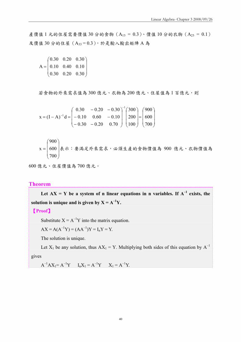
Linear Algebra- Chapter 3 20080926
40
產價值 1 元的住屋需要價值 30 分的食物(A13 = 03)價值 10 分的衣物(A23 = 01)
及價值 30 分的住屋(A33 = 03)於是輸入輸出矩陣 A 為
⎟⎟⎟
⎠
⎞
⎜⎜⎜
⎝
⎛=
300200300100400100300200300
A
若食物的外來需求值為 300 億元衣物為 200 億元住屋值為 1 百億元則
⎟⎟⎟
⎠
⎞
⎜⎜⎜
⎝
⎛=
⎟⎟⎟
⎠
⎞
⎜⎜⎜
⎝
⎛
⎟⎟⎟
⎠
⎞
⎜⎜⎜
⎝
⎛
minusminusminusminusminusminus
=minus=
minus
minus
700600900
100200300
700200300100600100300200300
d)AI(x
1
1
⎟⎟⎟
⎠
⎞
⎜⎜⎜
⎝
⎛=
700600900
x 表示要滿足外來需求必須生產的食物價值為 900 億元衣物價值為
600 億元住屋價值為 700 億元
Theorem
Let AX = Y be a system of n linear equations in n variables If Andash1 exists the
solution is unique and is given by X = Andash1Y
【Proof】
Substitute X = Andash1Y into the matrix equation
AX = A(Andash1Y) = (AAndash1)Y = InY = Y
The solution is unique
Let X1 be any solution thus AX1 = Y Multiplying both sides of this equation by Andash1
gives
Andash1AX1= Andash1Y InX1 = Andash1Y X1 = Andash1Y
Linear Algebra- Chapter 3 20080926
41
Example Example 1212
2x5x3x3x5x3x21x2x x
321
321
321
minus=++minus=minusminus=minusminus
⎥⎥⎥
⎦
⎤
⎢⎢⎢
⎣
⎡
minus=
⎥⎥⎥
⎦
⎤
⎢⎢⎢
⎣
⎡
⎥⎥⎥
⎦
⎤
⎢⎢⎢
⎣
⎡
minusminusminusminusminus
231
xxx
531532211
3
2
1
Solve the system of equations
This system can be written in the following matrix form
⎥⎥⎥
⎦
⎤
⎢⎢⎢
⎣
⎡
minus⎥⎥⎥
⎦
⎤
⎢⎢⎢
⎣
⎡
minusminusminusminusminus
=
⎥⎥⎥
⎦
⎤
⎢⎢⎢
⎣
⎡minus
231
531532211
xxx 1
3
2
1
If the matrix of coefficients is invertible the unique solutionIf the matrix of coefficients is invertible the unique solution isis
Example Example 2222
1 2 1 issolution unique The 321 =minus== xxx
⎥⎥⎥
⎦
⎤
⎢⎢⎢
⎣
⎡minus=
⎥⎥⎥
⎦
⎤
⎢⎢⎢
⎣
⎡
minus⎥⎥⎥
⎦
⎤
⎢⎢⎢
⎣
⎡
minusminusminus=
⎥⎥⎥
⎦
⎤
⎢⎢⎢
⎣
⎡
121
231
123135110
xxx
3
2
1
⎥⎥⎥
⎦
⎤
⎢⎢⎢
⎣
⎡
minusminusminus=
⎥⎥⎥
⎦
⎤
⎢⎢⎢
⎣
⎡
minusminusminusminusminus
=
minus
minus
123135110
531532211
A
1
1
The The LeontiefLeontief IO Model in IO Model in Economics Economics 1515
The Leontief input-output model is used to analyze the interdependence of economics Wassily Leontief received a Nobel Prize in 1973 for his work in thie fieldThe practical applications of this model have proliferated until it has now become a standard tool for investigating economic structures ranging from cities and corporation to states and countriesConsider an economics situation that involves ninterdependent industries The output of any one industry is needed as input by other industries and even possibly by the industry itself
The The LeontiefLeontief IO Model in IO Model in Economics Economics 2525
How a mathematical model involving a system of linear equations can be constructed to analyze such a situationAssume that each industry produces one commodity Let aij denote the amount of input of a certain commodity i to produce unit output of commodity j In our model let the amounts of input and output be measured in dollars Thus for example a34 = 045 means that 45 centsrsquo worth of commodity 3 is required to produce one dollarrsquos worth of commodity 4
The The LeontiefLeontief IO Model in IO Model in Economics Economics 3535
aij = amount of commodity i in one dollar of commodity jaij =生產一元價值的j產品需要耗用的i產品價值
The elements aij called input coefficients define a matrix A called the input-output matrix which describes the interdependence of the industriesExtending the model to include an open sector (all non-producing sectors) The product of industries may go not only into other producing industries but also into other non-producing sectors of the economy such as consumers and governments
The The LeontiefLeontief IO Model in IO Model in Economics Economics 4545
di = demand of the open sectors from industry ixi=total output of industry I necessary to meet demands of all n industries and the open sector
sectoropen of demand
nindustry of demand
2industry of demand
22
1industry of demand
11
industry ofoutput total
ininii
i
i dxaxaxax ++sdotsdotsdot++=
output ofportion sectoropen
output ofportion tryinterindusoutput total
DAXX +=Demand matrixDemand matrix
Output matrixOutput matrix
The The LeontiefLeontief IO Model in IO Model in Economics Economics 5555
Applying the model to the economy of a country X Applying the model to the economy of a country X represents the total output of each of the producing sectors represents the total output of each of the producing sectors of the economy and AX describes the contributions made of the economy and AX describes the contributions made by the various sectors to fulfilling the intersectional input by the various sectors to fulfilling the intersectional input requirements of the economyrequirements of the economyD is equal to (XD is equal to (X--AX) the difference between total output AX) the difference between total output X and industry transaction AXX and industry transaction AXD is thus the gross national product of the economyD is thus the gross national product of the economy
Example Example 1414
Consider an economy consisting of three industries having Consider an economy consisting of three industries having the following inputthe following input--output matrix output matrix AA Determine the output Determine the output levels required of the industries to meet the demands of levels required of the industries to meet the demands of the other industries and of the open sector in each casethe other industries and of the open sector in each case
in turn 321812
and 896
1612
9
5100
021
21
103
51
51
⎥⎥⎦
⎤
⎢⎢⎣
⎡
⎥⎥⎦
⎤
⎢⎢⎣
⎡
⎥⎥⎦
⎤
⎢⎢⎣
⎡=
⎥⎥⎥
⎦
⎤
⎢⎢⎢
⎣
⎡
= DA
The unit of The unit of DD are millions of dollarsare millions of dollars
Linear Algebra- Chapter 3 20080926
42
Example Example 2424
We wish to compute the output levels X that correspond to We wish to compute the output levels X that correspond to the various open sector demands D X is given by the the various open sector demands D X is given by the equation X = AX + D Rewritten as followsequation X = AX + D Rewritten as follows
X ndash AX = D rArr (I ndash A)X = D rArr X = (I ndash A) ndash1 D
⎥⎥⎥
⎦
⎤
⎢⎢⎢
⎣
⎡
=⎥⎥⎥
⎦
⎤
⎢⎢⎢
⎣
⎡
minus⎥⎥⎦
⎤
⎢⎢⎣
⎡=minus minus
minusminus
5400
021
21
103
51
54
5100
021
21
103
51
31
100010001
get We AI
⎥⎥⎥
⎦
⎤
⎢⎢⎢
⎣
⎡
=minus minus
4500
038
35
85
32
35
1)( AI
output ofingcorrespond valuesvarious
4500
038
35
85
32
35
)(
401020883957522133
32816189121269
)(
1
1
DAI
DAIX
minus
minus
minusuarruarruarruarruarruarruarr
⎥⎥⎦
⎤
⎢⎢⎣
⎡=
⎥⎥⎦
⎤
⎢⎢⎣
⎡
⎥⎥⎥
⎦
⎤
⎢⎢⎢
⎣
⎡
=minus=
Example Example 3434
By using Gauss-Jordan elimination
dollars of milliond are units The
40
15674
and 106629
209946
are 321812
and 896
1612
9
⎥⎥⎥
⎦
⎤
⎢⎢⎢
⎣
⎡
⎥⎥⎥
⎦
⎤
⎢⎢⎢
⎣
⎡
⎥⎥⎥
⎦
⎤
⎢⎢⎢
⎣
⎡
⎥⎥⎥
⎦
⎤
⎢⎢⎢
⎣
⎡
⎥⎥⎥
⎦
⎤
⎢⎢⎢
⎣
⎡
⎥⎥⎥
⎦
⎤
⎢⎢⎢
⎣
⎡
Example Example 4444
The output levels necessary to meet the demandsThe output levels necessary to meet the demands
IAAAIAI m =++++minus ))(( 2 L
mAAAIAI ++++=minus minus L21)(
Computing (IComputing (I--A) A) --11
1m
m2m2
m2
AI)AAAI(A)AAAI(I
)AAAI)(AI(
+minus=++++minus++++=
++++minusLL
L
NOTE 0A 1m rarr+
Population Movement Population Movement 1313
In 2000 58 million of people live in cities and 142 million of In 2000 58 million of people live in cities and 142 million of people people live in the surrounding suburbs Represent this information by tlive in the surrounding suburbs Represent this information by the he matrix matrix
The probability of a person staying in the city was 096 Thus tThe probability of a person staying in the city was 096 Thus the he probability of moving to the suburbs was 004 probability of moving to the suburbs was 004 The probability of a person moving to the city was 001 the The probability of a person moving to the city was 001 the probability of remaining in suburbia was 099probability of remaining in suburbia was 099
suburbcity
990040010960
suburbcity (to))from(
⎥⎦
⎤⎢⎣
⎡=P
⎥⎦
⎤⎢⎣
⎡=
14258
X0
City population in 2001 = people who remained from 2000 + peopleCity population in 2001 = people who remained from 2000 + peoplewho moved in from the suburbs = ( 096 who moved in from the suburbs = ( 096 timestimes 58 ) + (001 58 ) + (001 timestimes 142 ) = 142 ) = 571 million571 millionSuburban population in 2001 = people who moved in from the city Suburban population in 2001 = people who moved in from the city + people who stayed from 2000 = ( 004 + people who stayed from 2000 = ( 004 timestimes 58 ) + (099 58 ) + (099 timestimes 142 ) = 142 ) = 1429 million1429 millionCan arrive at these numbers using matrix multiplicationCan arrive at these numbers using matrix multiplication
⎥⎦
⎤⎢⎣
⎡=⎥
⎦
⎤⎢⎣
⎡⎥⎦
⎤⎢⎣
⎡==
9142157
14258
990040010960
PXX 01
Population Movement Population Movement 2323
Population Movement Population Movement 3333
Assume that the population flow represented by the matrix P is unchanged over the years The population distribution X2 after 2 years is given by X2 = P X1 = P2 X0 In general
Pn is called the n-step transition matrix The (ij)th element of Pngives the probability of going from state j to state i in n stepsFor example
in
ni XPX =+
suburbcity
960150040850
P
suburbcity (to))from(
4
⎥⎦
⎤⎢⎣
⎡=
The probability of living in the city in The probability of living in the city in 2000 and being in the suburbs 4 years 2000 and being in the suburbs 4 years later is 015later is 015
Markov ChainsMarkov Chains
The probabilities in the above model depend only on the The probabilities in the above model depend only on the current state of a person whether the person is living in the current state of a person whether the person is living in the city or in suburbiacity or in suburbiaThis type of model in which the probability of going from This type of model in which the probability of going from one state to another depends only on the current state one state to another depends only on the current state rather than on a more complete historical description is rather than on a more complete historical description is called a called a Markov chainMarkov chainMarkov chains are useful tools for scientists in many Markov chains are useful tools for scientists in many fields such as geneticsfields such as genetics
Linear Algebra- Chapter 3 20080926
43
GeneticsGenetics 1414
Genetics is the branch of biology that deals with Genetics is the branch of biology that deals with heredity heredity (遺傳)(遺傳) It is the study of units called It is the study of units called genes which determine the characteristics living genes which determine the characteristics living things inherit from their parents The inheritance things inherit from their parents The inheritance (遺傳)(遺傳)of such traitsof such traits(特徵)(特徵)as sex height eye as sex height eye color and hair color of human beings and such color and hair color of human beings and such traits as petaltraits as petal(花瓣)(花瓣) color and leaf shape of color and leaf shape of plants are governed by genesplants are governed by genesIn medicine agricultureIn medicine agriculturehelliphellip
GeneticsGenetics 2424
The traits of guinea pigsThe traits of guinea pigs(天竺鼠)(天竺鼠)are long hair and short hairare long hair and short hairThe length of hair is governed by a pair of gene which we denoteThe length of hair is governed by a pair of gene which we denote A A and aand aA guinea pig may have any one of the combination of AA A guinea pig may have any one of the combination of AA AaAa or or aaaa Each of these classes is called a genotypeEach of these classes is called a genotype(基因型)(基因型)The AA type guinea pig is indistinguishable in appearance from tThe AA type guinea pig is indistinguishable in appearance from the he AaAa type type ndashndash both have long hair both have long hair ndashndash whereas the whereas the aaaa type has short hairtype has short hairThe A gene is said to dominate the a geneThe A gene is said to dominate the a geneAn animal is called dominant An animal is called dominant (顯性)(顯性)if it has AA genes hybridif it has AA genes hybrid(混種)(混種) with with AaAa genes and recessive genes and recessive (隱性)(隱性)with with aaaa genesgenes
GeneticsGenetics 3434
When two guinea pigs are crossed the offspring inherits one genWhen two guinea pigs are crossed the offspring inherits one gene e from each parent in random mannerfrom each parent in random mannerGiven the genotype of the parents we can determine the Given the genotype of the parents we can determine the probabilities of the genotype of the offspringprobabilities of the genotype of the offspring
AA+AA AA+AA probabilities of AA probabilities of AA AaAa and and aaaa are 10and 0are 10and 0Aa+AAAa+AA probabilities of AA probabilities of AA AaAa and and aaaa are are frac12frac12 frac12frac12 and 0 and 0aa+AAaa+AA probabilities of AA probabilities of AA AaAa and and aaaa are 0 1 and 0are 0 1 and 0
This series of experiments is a Markov chain having transition This series of experiments is a Markov chain having transition matrixmatrix
aaAaAA
00012100211
P
aaAaAA
⎥⎥⎥
⎦
⎤
⎢⎢⎢
⎣
⎡=
GeneticsGenetics 4444
Assume an initial population of guinea pigs made up of an Assume an initial population of guinea pigs made up of an equal number of each genotypeequal number of each genotype
⎥⎥⎥
⎦
⎤
⎢⎢⎢
⎣
⎡=
313131
X0
The fractions of following generations are
⎥⎥⎥
⎦
⎤
⎢⎢⎢
⎣
⎡=
⎥⎥⎥
⎦
⎤
⎢⎢⎢
⎣
⎡=
⎥⎥⎥
⎦
⎤
⎢⎢⎢
⎣
⎡=
⎥⎥⎥
⎦
⎤
⎢⎢⎢
⎣
⎡=
01611615
X08187
X04143
X02121
X 4321
AAAAAaAaaaaa
3-4 Systems of Linear Equations ndash Computational Aspects
DEFINITION 36 Equivalent
Two systems of linear equations are called equivalent if they have the same solution
set
兩個線性方程組稱為等價意指兩者具有相同的解集合
Elementary Transformations Transformation called elementary transformations can be used to change a system of
linear equations into another system of linear equations that have the same solution
These transformations are used to solve system of linear equations by eliminating
variables
The equivalent transformations used in terms of matrix are called ELEMENTARY
ROW OPERATION
Linear Algebra- Chapter 3 20080926
44
Equivalent System Systems of equations that are related through elementary transformations are called
equivalent systems
Matrices that are related through elementary row operations are called row equivalent
matrices
The symbol asymp is used to indicate equivalence in both cases
Theorem 313 Let Ax = b be a system of m linear equations in n unknowns and let C be an invertible
mtimesm matrix Then the system (CA)x = Cb is equivalent to Ax = b
設 Ax = b 為含 n 個未知數m 個線性方程式的方程組若 C 為可逆的mtimesm
矩陣則(CA)x = Cb 等價於 Ax = b
【Proof】
Let K be the solution set for Ax = b and Krsquo the solution set for (CA)x = Cb If wisinK
then Aw = b So (CA)w = Cb and hence wisinKrsquo Thus KsubeKrsquo
Conversely if wisinKrsquo then (CA)w = Cb Hence Aw = C-1(CA)w = C-1(Cb) = b so
wisinK Thus KrsquosubeK and therefore K=Krsquo
設 K 為 Ax = b 的解集合且 Krsquo為(CA)x = Cb 的解集合
若 wisinK則 Aw = b (CA)w = Cb故 wisinKrsquo於是 KsubeKrsquo
反之若 wisinKrsquo則(CA)w = Cb Aw = C-1(CA)w = C-1(Cb) = b故 wisinK於是
KrsquosubeK因此K=Krsquo
Corollary Let Ax = b be a system of m linear equations in n unknowns If (Arsquo brsquo) is obtained ∣
from from (A b) by a finite number of elementary row operations then the system Arsquox = ∣
brsquo is equivalent to the original system
設 Ax = b 為含 n 個未知數m 個線性方程式的方程組若(Arsquo brsquo) ∣ 是由(A b) ∣
經過有限次數的基本列運算而得則 Arsquox = brsquo 等價於 Ax = b即兩者具有相同的解
集合
【Proof】
Suppose that (Arsquo brsquo) is obtained from (A b) by elementary row operations These ∣ ∣
Linear Algebra- Chapter 3 20080926
45
may be executed by multiplying (A b) by elementary mtimesm matrices E∣ 1 E2hellipEp Let
C=EphellipE2E1 then (Arsquo brsquo) = C(A b) = (CA Cb)∣ ∣ ∣
Since each Ei is invertible so is C Now Arsquo = CA and brsquo = Cb Thus by Theorem 313
the system Arsquox = brsquo is equivalent to the system Ax = b
設(Arsquo brsquo)∣ 是由(A b)∣ 經過基本列運算取得即以基本 mtimesm 矩陣 E1 E2hellipEp
乘上 (A b)∣ (Arsquo brsquo) = C(A b) = (CA Cb∣ ∣ ∣ )其中C=EphellipE2E1
因 Ei 可逆故 C 亦為可逆 Arsquo = CA 且 brsquo = Cb
依據 Theorem 313Arsquox = brsquo 等價於 Ax = b
Theorem 313 Let Ax = b be a system of m linear equations in n unknowns and let C be an
invertible mtimesm matrix Then the system (CA)x = Cb is equivalent to Ax = b 設 Ax = b
為含 n 個未知數m 個線性方程式的方程組若 C 為可逆的mtimesm 矩陣則(CA)x
= Cb 等價於 Ax = b
We now describe a method for solving any stystem of linear equations Consider for
example the system of linear equations
探討解線性方程組的方法hellip
2xxx2x3xxx1x2x3x2x3
4321
321
4321
=minus++=++=minus++
First we form the augmented matrix ⎟⎟⎟
⎠
⎞
⎜⎜⎜
⎝
⎛
minus
minus
231
112101112323
(增廣矩陣)
Interchanging the first and third rows ⎟⎟⎟
⎠
⎞
⎜⎜⎜
⎝
⎛
minus
minus
132
132301111121
(第 13 列互調)
Adding -1 times the first row to the second row and then add -3 times the first row to
the third row ⎟⎟⎟
⎠
⎞
⎜⎜⎜
⎝
⎛
minusminusminus
minus
512
104010101121
(第 1 列乘上 -1 加到第 2 列再以 -3 乘上
第 1 列加到第 3 列)
Linear Algebra- Chapter 3 20080926
46
Multiplying the second row by -1 ⎟⎟⎟
⎠
⎞
⎜⎜⎜
⎝
⎛
minusminus
minusminusminus
51
2
104010101121
(第 2 列乘上 -1)
Adding four times the second row to the third row ⎟⎟⎟
⎠
⎞
⎜⎜⎜
⎝
⎛
minusminus
minusminusminus
91
2
300010101121
(4 乘上第 2
列加到第 3 列)
Multiplying the third row by -13 ⎟⎟⎟
⎠
⎞
⎜⎜⎜
⎝
⎛minusminus
minus
31
2
100010101121
(第 3 列乘上 -13)
Adding the third row to the first and second rows to obtain zeros in row 1 column 4
and row 2 column 4 ⎟⎟⎟
⎠
⎞
⎜⎜⎜
⎝
⎛
325
100000100121
(將第 3 列加到第 1 列及第 2 列)
Adding -2 times the second row to the first row in order to make the first row second
column entry become zero ⎟⎟⎟
⎠
⎞
⎜⎜⎜
⎝
⎛
321
100000100101
(將第 2 列乘以 -2 再加至第 1 列)
We have now obtained the desired reduction of the augmented matrix
⎟⎟⎟
⎠
⎞
⎜⎜⎜
⎝
⎛
321
100000100101
是化簡後的增廣矩陣
This matrix corresponds to the system of linear equations
對應的線性方程組為
2x3x1xx
4
2
31
===+
By Corollary to Theorem 313 this system is equivalent to the original system But this
system is easily solved Obviously x2 = 2 and x4 = 3 Moreover x1 and x3 can be any values
Linear Algebra- Chapter 3 20080926
47
provided their sum is 1 Letting x3 = t we then have x1 = 1 ndash t Thus an arbitray solution to the
original system has the form
依據 Corollary to Theorem 313 化簡後的方程組與原方程組等值此方程組的解為
x2 = 3x4 = 3x1 + x3 = 1於是原方程組的任意解可以寫成
⎟⎟⎟⎟⎟
⎠
⎞
⎜⎜⎜⎜⎜
⎝
⎛minus
+
⎟⎟⎟⎟⎟
⎠
⎞
⎜⎜⎜⎜⎜
⎝
⎛
=
⎟⎟⎟⎟⎟
⎠
⎞
⎜⎜⎜⎜⎜
⎝
⎛ minus
0101
t
3021
3t2
t1
Observe that
⎪⎪⎭
⎪⎪⎬
⎫
⎪⎪⎩
⎪⎪⎨
⎧
⎟⎟⎟⎟⎟
⎠
⎞
⎜⎜⎜⎜⎜
⎝
⎛minus
0101
is a basis for the homogeneous system of equations
corresponding to the given system
其中
⎪⎪⎭
⎪⎪⎬
⎫
⎪⎪⎩
⎪⎪⎨
⎧
⎟⎟⎟⎟⎟
⎠
⎞
⎜⎜⎜⎜⎜
⎝
⎛minus
0101
是齊次方程組解集合的一組基底
Gauss-Jordan Elimination
Let A be an n times n matrix
1 Adjoin the identity n times n matrix In to A to form the matrix [A In]
2 Compute the reduced echelon form of [A In]
(1) If the reduced echelon form is of the type [In B] then B is the inverse of A
(2) If the reduced echelon form is not of the type [In B] in that the first n times n
submatrix is not In then A has no inverse
An n times n matrix A is invertible if and only if its reduced echelon form is In
DEFINITION 37 Reduced Row Echelon Form
A matrix is said to be in reduced row echelon form if the following three conditions
are satisfied
Linear Algebra- Chapter 3 20080926
48
一個矩陣可以被稱為簡約列梯形式必須具備有下列三條件
(a) Any row containing a nonzero entry preceeds any row in which all the entries are
zero (if any)
含有非零元素的任一列排在全含零元素的任一列前面(儘可能)
(b) The first nonzero entry in each row in the only nonzero entry in its column
各列中第一個非零元素為其所在行中唯一的非零元素
(c) The first nonzero entry in each row is 1 and it occurs in a column to thr right of the
first nonzero entry in the preceeding row
各列中第一個非零元素為 1 且它出現在前一列中第一個非零元素的右邊某一
行中
Reduced Echelon Form A matrix is in reduced echelon form if
1 Any rows consisting entirely of zeros are grouped at the bottom of the matrix
2 The first nonzero element of each other row is 1 This element is called a leading 1
3 The leading 1 of each row after the first is positioned to the right of the leading 1 of
the previous row
4 All other elements in a column that contains a leading 1 are zero
Theorem 314 Gaussian Elimination Transformation Gaussian elimination transform any matrix into its reduced row echelon form
利用 Gaussian elimination 將矩陣轉換成簡約列梯形式
We now describe a method for solving a system in which the augmented matrix is in
reduced row echelon form To illustrate this procedure we consider the system
14x8x3x2x2x28x5x2xxx6x3xxxx17x9x4xx3x2
54321
54321
54321
54321
=minus+++=minus+++=minus+++=minus+++
Linear Algebra- Chapter 3 20080926
49
for which the augmented matrix is
⎟⎟⎟⎟⎟
⎠
⎞
⎜⎜⎜⎜⎜
⎝
⎛
minusminusminusminus
1486
17
83222521113111194132
(增廣矩陣)
Applying Gaussian elimination to the augmented matrix of the system produces the
following sequence of matrices
利用 Gaussian elimination method 處理增廣矩陣
⎟⎟⎟⎟⎟
⎠
⎞
⎜⎜⎜⎜⎜
⎝
⎛
minusminusminusminus
1486
17
83222521113111194132
⎟⎟⎟⎟⎟
⎠
⎞
⎜⎜⎜⎜⎜
⎝
⎛
minusminusminusminus
148
176
83222521119413231111
⎟⎟⎟⎟⎟
⎠
⎞
⎜⎜⎜⎜⎜
⎝
⎛
minusminus
minus
0213
0000021000
1011020201
The system of linear equations corresponding to thus last matrix is
對應最後矩陣的線性方程組 2x2x
1xxx3x2x2x
54
532
531
=minus=+minus=minus+
Assign x3 = t1 x5 = t2
2t22x2x1tt1xxx
3t2t23x2x2x
254
21532
21531
+=+=+minus=+minus=
++minus=++minus=
Thus an arbitray solution s is of the form
於是任意解 s 具有下列形式
s =
⎟⎟⎟⎟⎟⎟
⎠
⎞
⎜⎜⎜⎜⎜⎜
⎝
⎛minus
+
⎟⎟⎟⎟⎟⎟
⎠
⎞
⎜⎜⎜⎜⎜⎜
⎝
⎛minus
+
⎟⎟⎟⎟⎟⎟
⎠
⎞
⎜⎜⎜⎜⎜⎜
⎝
⎛
=
⎟⎟⎟⎟⎟⎟
⎠
⎞
⎜⎜⎜⎜⎜⎜
⎝
⎛
+
+minus++minus
=
⎟⎟⎟⎟⎟⎟
⎠
⎞
⎜⎜⎜⎜⎜⎜
⎝
⎛
1201
2
t
00112
t
02013
t2t2
t1tt
3t2t2
xxxxx
21
2
2
1
21
21
5
4
3
2
1
where t1t2isinR
Linear Algebra- Chapter 3 20080926
50
Notice that
⎪⎪⎪
⎭
⎪⎪⎪
⎬
⎫
⎪⎪⎪
⎩
⎪⎪⎪
⎨
⎧
⎟⎟⎟⎟⎟⎟
⎠
⎞
⎜⎜⎜⎜⎜⎜
⎝
⎛minus
⎟⎟⎟⎟⎟⎟
⎠
⎞
⎜⎜⎜⎜⎜⎜
⎝
⎛minus
1201
2
00112
is a basis for the solution set of the corresponding
homogeneous system of equation and
⎟⎟⎟⎟⎟⎟
⎠
⎞
⎜⎜⎜⎜⎜⎜
⎝
⎛
02013
is a particular solution to the original system
⎪⎪⎪
⎭
⎪⎪⎪
⎬
⎫
⎪⎪⎪
⎩
⎪⎪⎪
⎨
⎧
⎟⎟⎟⎟⎟⎟
⎠
⎞
⎜⎜⎜⎜⎜⎜
⎝
⎛minus
⎟⎟⎟⎟⎟⎟
⎠
⎞
⎜⎜⎜⎜⎜⎜
⎝
⎛minus
1201
2
00112
是齊次方程組解集合的一組基底
⎟⎟⎟⎟⎟⎟
⎠
⎞
⎜⎜⎜⎜⎜⎜
⎝
⎛
02013
是原方程組的特別解
EXAMPLE 1
The matrix ⎟⎟⎟
⎠
⎞
⎜⎜⎜
⎝
⎛
101010011
is not in reduced row echelon form
因為第一行含有第一個非零元素在第一列但第一行尚含有其他非零元素
The matrix ⎟⎟⎟
⎠
⎞
⎜⎜⎜
⎝
⎛
110010012010
is not in reduced row echelon form
因為第一列第一個非零元素不在第一列第一個非零元素的右邊
The matrix ⎟⎟⎠
⎞⎜⎜⎝
⎛010002
is not in reduced row echelon form
因為第一列的第一個非零元素不是 1
Linear Algebra- Chapter 3 20080926
51
Reduced Echelon FormReduced Echelon Form
⎥⎥⎥
⎦
⎤
⎢⎢⎢
⎣
⎡
910030107001
⎥⎥⎥
⎦
⎤
⎢⎢⎢
⎣
⎡
100001000041
⎥⎥⎥
⎦
⎤
⎢⎢⎢
⎣
⎡
000210801
Not in Reduced Echelon Form
⎥⎥⎥
⎦
⎤
⎢⎢⎢
⎣
⎡
310000004021
⎥⎥⎥
⎦
⎤
⎢⎢⎢
⎣
⎡
100000430003021
⎥⎥⎥⎥
⎦
⎤
⎢⎢⎢⎢
⎣
⎡
0000210030108071
In Reduced Echelon Form
Use GaussUse Gauss--Jordan elimination to Jordan elimination to find reduced echelon formfind reduced echelon form 1313
Step 1 Interchange rows if necessary to bring a nonzero Step 1 Interchange rows if necessary to bring a nonzero element to the top of the first nonzero column This nonzero element to the top of the first nonzero column This nonzero element is called a pivotelement is called a pivot
⎥⎥⎦
⎤
⎢⎢⎣
⎡
minusminus
minus
1211244129333
22200
⎥⎥⎥
⎦
⎤
⎢⎢⎢
⎣
⎡
minusminus
minus
harrasymp
121124422200
129333
R2R1
Use GaussUse Gauss--Jordan elimination to Jordan elimination to find reduced echelon formfind reduced echelon form 2323
Step 2 Create a 1 in the pivot location by multiplying the Step 2 Create a 1 in the pivot location by multiplying the pivot row by 1pivotpivot row by 1pivot
Step 3 Create zero elsewhere in the pivot column by adding Step 3 Create zero elsewhere in the pivot column by adding suitable multiples of the pivot row to all other rows of the suitable multiples of the pivot row to all other rows of the matrixmatrix
⎥⎥⎥
⎦
⎤
⎢⎢⎢
⎣
⎡
minusminusminus
minus
minus+asymp
412002220043111
4)R1(R3
⎥⎥⎦
⎤
⎢⎢⎣
⎡
minusminus
minus
⎟⎠⎞
⎜⎝⎛asymp
12112442220043111
R13
1
The matrix is the reduced echelon form of the given matrixThe matrix is the reduced echelon form of the given matrix
Use GaussUse Gauss--Jordan elimination to Jordan elimination to find reduced echelon formfind reduced echelon form 3333
Step 4 Cover the pivot row and all rows above it Repeat Steps Step 4 Cover the pivot row and all rows above it Repeat Steps 1 1 and 2 for the remaining and 2 for the remaining submatrixsubmatrix Repeat Step 3 for the whole Repeat Step 3 for the whole matrix Continue until the reduced echelon form is reachedmatrix Continue until the reduced echelon form is reached
⎥⎥⎥
⎦
⎤
⎢⎢⎢
⎣
⎡
minusminus
+minus+asymp
⎥⎥⎥
⎦
⎤
⎢⎢⎢
⎣
⎡
minusminus
minus++asymp
⎥⎥⎥
⎦
⎤
⎢⎢⎢
⎣
⎡
minusminusminus
minus
⎟⎠⎞
⎜⎝⎛
asymp
⎥⎥⎥
⎦
⎤
⎢⎢⎢
⎣
⎡
minusminusminus
minus
6100050100
170011
R3R22)R3(R1
610001110052011
R2)2(R3R2R1
412001110043111
R221
412002220043111
Theorem 315 Let Ax = b be a system of r nonzero equations is in n unknown Suppose that rank(A)
= rank (A b)∣ and that (A b)∣ is in reduced row echelon form Then
設 Ax = b 為含有 n 個未知數r 個非零方程式的方程組假設 rank(A) = rank
(A b)∣ 且 (A b)∣ 為簡約列梯形式於是
(a) rank(A) = r
(b) If the general solution obtained by the procedure above is of the form s = s0 + t1u1
+ t2u2 +hellip+ tn-run-r then u1 u2hellip un-r is a basis for the solution set of the
corresponding homogeneous system and s0 is a solution to the original system 由
前述方法所得的 General solution 具有下列形式
s = s0 + t1u1 + t2u2 +hellip+ tn-run-r
其中u1 u2hellip un-r為齊次方程組 Ax = 0 的解集合的一組基底且 s0 為原方
程組的一個解)
【Proof】
Since (A b)∣ is in reduced row echelon form (A b)∣ must have r nonzero rows
Clearly these rows are linearly independent by the definition of the reduced row echelon
Linear Algebra- Chapter 3 20080926
52
form and so rank (A b)∣ = r Thus rank(A) = r
Let K be the solution set for Ax = b and let KH be the solution set for Ax = 0 Setting
t1 = t2 =hellip= tn-r = 0 we see that s = s0isinK But by Theorem 39 K = s +KH Hence
KH = - s0+K = span(u1 u2hellip un-r )
Because rank(A) = r we have dim(KH) = n-r Thus since dim(KH) = n-r and KH is
generated by a set u1 u2hellip un-r containing at most n-r vectors that is a basis for KH
由於(A b)∣ 具有簡約列梯形式因此(A b)∣ 必定具有 r 個非零列由簡約列梯形
式的定義得知 r 個非零列為線性獨立故 rank (A b)∣ = rrank(A) = r
令 K 為 Ax = b 的解集合 KH 為 Ax = 0 的解集合
假設 t1 = t2 =hellip= tn-r = 0(u1 u2hellip un-r非 KH的基底)則 s = s0isinK
依據 Theorem 39K = s +KH KH = - s0+K = span(u1 u2hellip un-r )
因 rank(A) = r所以 dim(KH) = n - r 且 KH 是由u1 u2hellip un-r 所生成
故原假設「t1 = t2 =hellip= tn-r = 0」不成立
因此 KH含有最多 n - r 個向量且這些向量為 KH的基底
Theorem 39 Let K be the solution set of a system of linear equations Ax = b and let KH be
the solution set of the corresponding homogeneous system Ax = 0 Then for any solution s
to Ax = b K =s + KH = s+k kisinKH 設 K 為線性方程組 Ax = b 的解集合且 KH
為對應的齊次方程組的解集合則對 Ax = b 的任一個解 s 而言K =s + KH = s+k
kisinKH
ExampleExampleSolve the system of equationsSolve the system of equations
7537429333
321
321
321
=minusminus=+minus=+minus
xxxxxxxxx
⎥⎥⎦
⎤
⎢⎢⎣
⎡
++asymp
000012104301
R2R3R2R1 12
431243
32
31
32
31+minus=+minus=rArr=+
=+rArr xxxx
xxxx
The general solution to the system isThe general solution to the system is
parameter) a (callednumber real is where 1243
3
2
1
rrxrxrx
=+minus=+minus=
⎥⎥⎥
⎦
⎤
⎢⎢⎢
⎣
⎡
minusminusminus
minus
minus+minus+asymp
⎥⎥⎥
⎦
⎤
⎢⎢⎢
⎣
⎡
minusminusminusminus
asymp
⎥⎥⎥
⎦
⎤
⎢⎢⎢
⎣
⎡
minusminusminusminus
242012103111
1R)3(3R1R)2(2R
715374123111
715374129333
R131
ExampleExample
Solve the system of equationsSolve the system of equations446942
1423258101242
4321
4321
4321
=minus+minusminus=+minus+minus
=minus+minus
xxxxxxxxxxxx
⎪⎪
⎩
⎪⎪
⎨
⎧
===
minus=
rArr==minus=minus
rArr
1x6xrx
2r2x
1x6x
2x2x
4
3
2
1
4
3
21
⎥⎥⎥
⎦
⎤
⎢⎢⎢
⎣
⎡ minusminusasymp
⎥⎥⎥
⎦
⎤
⎢⎢⎢
⎣
⎡minus
minusminusasymp
⎥⎥⎥
⎦
⎤
⎢⎢⎢
⎣
⎡
minusminusminusminusminusasymp
⎥⎥⎥
⎦
⎤
⎢⎢⎢
⎣
⎡
minusminusminusminusminusasymp
⎥⎥⎥
⎦
⎤
⎢⎢⎢
⎣
⎡
minusminusminusminusminus
minusminusasymp
⎥⎥⎥
⎦
⎤
⎢⎢⎢
⎣
⎡
minusminusminusminusminus
minusminus
+
minus+
+
minus+
minus+
+
110006010020021
110005110011021
14430051100
295621
2R31
144300153300295621
446942142321295621
44694214232158101242
R3R2
1)R3(R1
3R2R3
6)R2(R1
2)R1(R3
R1R2R1
21
Linear Algebra- Chapter 3 20080926
53
ExampleExampleSolve the system of equationsSolve the system of equations
432636242232
54321
54321
54321
=+minus+minusminus=++minus+=++minus+
xxxxxxxxxxxxxxx
⎥⎥⎦
⎤
⎢⎢⎣
⎡ minusasymp
⎥⎥⎦
⎤
⎢⎢⎣
⎡
minusminusminusminusminus
+
minus+
642000210000213121
431121636242213121
R1R3
2)R1(R2
⎥⎥⎦
⎤
⎢⎢⎣
⎡ minusasympharr 210000
642000213121
R3R2 ( ) ⎥⎥⎦
⎤
⎢⎢⎣
⎡ minusasymp
210000321000213121
2R21
⎥⎥⎦
⎤
⎢⎢⎣
⎡ minusminusminusasympminus+ 210000
321000750121
3)R2(R1 ⎥⎥⎦
⎤
⎢⎢⎣
⎡minus
minusasymp
minus+
+
210000101000300121
2)R3(R2
5R3R1
2x1x
3xx2x
5
4
321
=minus=
++minus=rArr
2xs and r somefor 1x sx rx
3sr2x
5
432
1
=minus===
++minus=
ExampleExample
Solve the system of Solve the system of equationsequations 122
32452232
32
321
321
321
=+minus=minus+
=+minus=+minus
xxxxxxxxxxx
⎥⎥
⎦
⎤
⎢⎢
⎣
⎡asymp
minusminusminus
minus
harr1220210063303211
R3R2
( ) ⎥⎥
⎦
⎤
⎢⎢
⎣
⎡asymp
minusminusminus
minus
1220210021103211
R231
⎥⎥
⎦
⎤
⎢⎢
⎣
⎡asympminusminusminus
minus+
+
5400210021101101
2)R2(R4
R2R1 ⎥⎥
⎦
⎤
⎢⎢
⎣
⎡asymp
minusminus
minus+
+
minus+
13000210040103001
4)R3R(R4
R3R2
1)R3(R1
( ) ⎥⎥
⎦
⎤
⎢⎢
⎣
⎡asymp
minusminus
1000210040103001
R4131
The system has no solutionThe system has no solution
⎥⎥
⎦
⎤
⎢⎢
⎣
⎡asymp
⎥⎥
⎦
⎤
⎢⎢
⎣
⎡
minusminusminus
minus
minusminusminusminus
minus+
minus+
1220633021003211
1220312145223211
1)R1(R3
2)R1(R2
0x1+0x2+0x3=1
Curve FittingCurve Fitting
A set of data points A set of data points is given and it is is given and it is necessary to find a polynomial whose graph passes through the necessary to find a polynomial whose graph passes through the points points The points are often measurements in an experiment The points are often measurements in an experiment The xThe x--coordinates are called coordinates are called base pointsbase pointsIt can be shown that if the base points are all distinct then aIt can be shown that if the base points are all distinct then a unique unique polynomial of degree n polynomial of degree n ndashndash 1 (or less)1 (or less)
can be fitted to thecan be fitted to the pointspoints
) ( ) ( ) ( 2211 nn yxyxyx K
11
2210
minusminus
minusminus ++++= n
nn
n xaxaxaay K
The coefficients can be found by substituting the points The coefficients can be found by substituting the points into the polynomial equation and then solving a system into the polynomial equation and then solving a system of linear equationsof linear equations
ExampleExample
Determine the equation of the polynomial of degree 2 whose graphpasses through the points (1 6) (2 3) (3 2)
Let the polynomial be and substituting x = 1 y = 6 x = 2 y = 3 x = 3 y = 2 we have
Solving this system for a0 a1 and a2 using Gauss-Jordan elimination
⎥⎥⎥
⎦
⎤
⎢⎢⎢
⎣
⎡minus
minus
minus+minus+asymp
220033109201
1)R2(R31)R2(R1
2210 xaxaay ++=
2a9a3a3a4a2a6aaa
210
210
210
=++=++=++
⎥⎥⎥
⎦
⎤
⎢⎢⎢
⎣
⎡
minusminus
⎥⎥⎥
⎦
⎤
⎢⎢⎢
⎣
⎡
minus+minus+asymp
482033106111
293134216111
1)R1(R31)R1(R2
( )⎥⎥⎥
⎦
⎤
⎢⎢⎢
⎣
⎡minus
⎥⎥⎥
⎦
⎤
⎢⎢⎢
⎣
⎡minus
minusasymp
minus++asymp
11006010
11001
110033109201
3)R3(R22R3R1
R321
We get a0 = 11 a1 = ndash 6 a2 = 1The parabola that passes through these points is y = 11 ndash 6x + x2
ExampleExample Traffic FlowTraffic Flow
Network analysis plays an important role in electrical Network analysis plays an important role in electrical engineeringengineeringThe concepts and tools of network analysis have been The concepts and tools of network analysis have been found to be useful in many other fields such as found to be useful in many other fields such as information theory and the study of transportation systemsinformation theory and the study of transportation systemsThe analysis of traffic flow through a road network during The analysis of traffic flow through a road network during peak period illustrates how systems of linear equations peak period illustrates how systems of linear equations with with manymany solutions can arise in practicesolutions can arise in practice
Traffic FlowTraffic Flow
Consider the typical road network The streets are all oneConsider the typical road network The streets are all one--way with the arrows indicating the direction of traffic flowway with the arrows indicating the direction of traffic flowThe flow of traffic in and out of the network is measured The flow of traffic in and out of the network is measured in vehicles per hour (in vehicles per hour (vphvph))How to construct a mathematical model to analyze this How to construct a mathematical model to analyze this network network
Traffic Traffic FlowFlowTRAFFIC LAWTRAFFIC LAWhelliphellipAll traffic entering an intersection must leave that All traffic entering an intersection must leave that intersectionintersection
Linear Algebra- Chapter 3 20080926
54
Junction AJunction BJunction CJunction DJunction EJunction F 600
800 200 500 100 600
54
643
73
72
621
51
=+=++minus=+minus=minus=+minus=+
xxxxx
xxxx
xxxxx
⎥⎥⎥⎥⎥⎥⎥⎥⎥⎥⎥⎥⎥
⎦
⎤
⎢⎢⎢⎢⎢⎢⎢⎢⎢⎢⎢⎢⎢
⎣
⎡
asympasymp
⎥⎥⎥⎥⎥⎥⎥⎥⎥⎥⎥⎥⎥
⎦
⎤
⎢⎢⎢⎢⎢⎢⎢⎢⎢⎢⎢⎢⎢
⎣
⎡
minusminus
minusminusminusminus
minusminus
minusminus
0000000001110000
6001101000200100010050010000106001100001
600001100080001011002001000100500100001010001000116000010001
L
Traffic FlowTraffic FlowJunction AJunction BJunction CJunction DJunction EJunction F 600
800 200 500 100 600
54
643
73
72
621
51
=+=++minus=+minus=minus=+minus=+
xxxxx
xxxx
xxxxx
Perform road work on x7 Because x3 ge 0 the minimum flow 200 in the branch x7 can be obtained by making x3 = 0 (closing DE to traffic)
Traffic FlowTraffic Flow
We get
765
76473
72761
xx x600xxx200x x500x x600xxx
minus=++minus=minus=+=+minusminus=
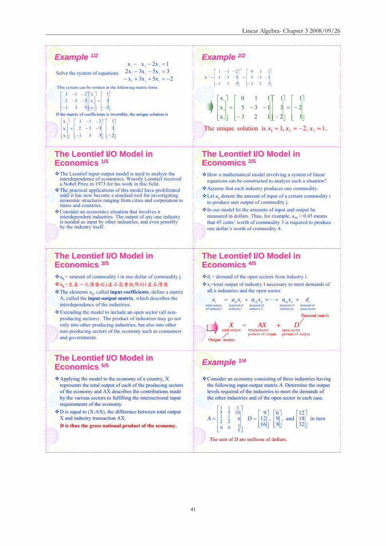
Linear Algebra- Chapter 3 20080926
43
GeneticsGenetics 1414
Genetics is the branch of biology that deals with Genetics is the branch of biology that deals with heredity heredity (遺傳)(遺傳) It is the study of units called It is the study of units called genes which determine the characteristics living genes which determine the characteristics living things inherit from their parents The inheritance things inherit from their parents The inheritance (遺傳)(遺傳)of such traitsof such traits(特徵)(特徵)as sex height eye as sex height eye color and hair color of human beings and such color and hair color of human beings and such traits as petaltraits as petal(花瓣)(花瓣) color and leaf shape of color and leaf shape of plants are governed by genesplants are governed by genesIn medicine agricultureIn medicine agriculturehelliphellip
GeneticsGenetics 2424
The traits of guinea pigsThe traits of guinea pigs(天竺鼠)(天竺鼠)are long hair and short hairare long hair and short hairThe length of hair is governed by a pair of gene which we denoteThe length of hair is governed by a pair of gene which we denote A A and aand aA guinea pig may have any one of the combination of AA A guinea pig may have any one of the combination of AA AaAa or or aaaa Each of these classes is called a genotypeEach of these classes is called a genotype(基因型)(基因型)The AA type guinea pig is indistinguishable in appearance from tThe AA type guinea pig is indistinguishable in appearance from the he AaAa type type ndashndash both have long hair both have long hair ndashndash whereas the whereas the aaaa type has short hairtype has short hairThe A gene is said to dominate the a geneThe A gene is said to dominate the a geneAn animal is called dominant An animal is called dominant (顯性)(顯性)if it has AA genes hybridif it has AA genes hybrid(混種)(混種) with with AaAa genes and recessive genes and recessive (隱性)(隱性)with with aaaa genesgenes
GeneticsGenetics 3434
When two guinea pigs are crossed the offspring inherits one genWhen two guinea pigs are crossed the offspring inherits one gene e from each parent in random mannerfrom each parent in random mannerGiven the genotype of the parents we can determine the Given the genotype of the parents we can determine the probabilities of the genotype of the offspringprobabilities of the genotype of the offspring
AA+AA AA+AA probabilities of AA probabilities of AA AaAa and and aaaa are 10and 0are 10and 0Aa+AAAa+AA probabilities of AA probabilities of AA AaAa and and aaaa are are frac12frac12 frac12frac12 and 0 and 0aa+AAaa+AA probabilities of AA probabilities of AA AaAa and and aaaa are 0 1 and 0are 0 1 and 0
This series of experiments is a Markov chain having transition This series of experiments is a Markov chain having transition matrixmatrix
aaAaAA
00012100211
P
aaAaAA
⎥⎥⎥
⎦
⎤
⎢⎢⎢
⎣
⎡=
GeneticsGenetics 4444
Assume an initial population of guinea pigs made up of an Assume an initial population of guinea pigs made up of an equal number of each genotypeequal number of each genotype
⎥⎥⎥
⎦
⎤
⎢⎢⎢
⎣
⎡=
313131
X0
The fractions of following generations are
⎥⎥⎥
⎦
⎤
⎢⎢⎢
⎣
⎡=
⎥⎥⎥
⎦
⎤
⎢⎢⎢
⎣
⎡=
⎥⎥⎥
⎦
⎤
⎢⎢⎢
⎣
⎡=
⎥⎥⎥
⎦
⎤
⎢⎢⎢
⎣
⎡=
01611615
X08187
X04143
X02121
X 4321
AAAAAaAaaaaa
3-4 Systems of Linear Equations ndash Computational Aspects
DEFINITION 36 Equivalent
Two systems of linear equations are called equivalent if they have the same solution
set
兩個線性方程組稱為等價意指兩者具有相同的解集合
Elementary Transformations Transformation called elementary transformations can be used to change a system of
linear equations into another system of linear equations that have the same solution
These transformations are used to solve system of linear equations by eliminating
variables
The equivalent transformations used in terms of matrix are called ELEMENTARY
ROW OPERATION
Linear Algebra- Chapter 3 20080926
44
Equivalent System Systems of equations that are related through elementary transformations are called
equivalent systems
Matrices that are related through elementary row operations are called row equivalent
matrices
The symbol asymp is used to indicate equivalence in both cases
Theorem 313 Let Ax = b be a system of m linear equations in n unknowns and let C be an invertible
mtimesm matrix Then the system (CA)x = Cb is equivalent to Ax = b
設 Ax = b 為含 n 個未知數m 個線性方程式的方程組若 C 為可逆的mtimesm
矩陣則(CA)x = Cb 等價於 Ax = b
【Proof】
Let K be the solution set for Ax = b and Krsquo the solution set for (CA)x = Cb If wisinK
then Aw = b So (CA)w = Cb and hence wisinKrsquo Thus KsubeKrsquo
Conversely if wisinKrsquo then (CA)w = Cb Hence Aw = C-1(CA)w = C-1(Cb) = b so
wisinK Thus KrsquosubeK and therefore K=Krsquo
設 K 為 Ax = b 的解集合且 Krsquo為(CA)x = Cb 的解集合
若 wisinK則 Aw = b (CA)w = Cb故 wisinKrsquo於是 KsubeKrsquo
反之若 wisinKrsquo則(CA)w = Cb Aw = C-1(CA)w = C-1(Cb) = b故 wisinK於是
KrsquosubeK因此K=Krsquo
Corollary Let Ax = b be a system of m linear equations in n unknowns If (Arsquo brsquo) is obtained ∣
from from (A b) by a finite number of elementary row operations then the system Arsquox = ∣
brsquo is equivalent to the original system
設 Ax = b 為含 n 個未知數m 個線性方程式的方程組若(Arsquo brsquo) ∣ 是由(A b) ∣
經過有限次數的基本列運算而得則 Arsquox = brsquo 等價於 Ax = b即兩者具有相同的解
集合
【Proof】
Suppose that (Arsquo brsquo) is obtained from (A b) by elementary row operations These ∣ ∣
Linear Algebra- Chapter 3 20080926
45
may be executed by multiplying (A b) by elementary mtimesm matrices E∣ 1 E2hellipEp Let
C=EphellipE2E1 then (Arsquo brsquo) = C(A b) = (CA Cb)∣ ∣ ∣
Since each Ei is invertible so is C Now Arsquo = CA and brsquo = Cb Thus by Theorem 313
the system Arsquox = brsquo is equivalent to the system Ax = b
設(Arsquo brsquo)∣ 是由(A b)∣ 經過基本列運算取得即以基本 mtimesm 矩陣 E1 E2hellipEp
乘上 (A b)∣ (Arsquo brsquo) = C(A b) = (CA Cb∣ ∣ ∣ )其中C=EphellipE2E1
因 Ei 可逆故 C 亦為可逆 Arsquo = CA 且 brsquo = Cb
依據 Theorem 313Arsquox = brsquo 等價於 Ax = b
Theorem 313 Let Ax = b be a system of m linear equations in n unknowns and let C be an
invertible mtimesm matrix Then the system (CA)x = Cb is equivalent to Ax = b 設 Ax = b
為含 n 個未知數m 個線性方程式的方程組若 C 為可逆的mtimesm 矩陣則(CA)x
= Cb 等價於 Ax = b
We now describe a method for solving any stystem of linear equations Consider for
example the system of linear equations
探討解線性方程組的方法hellip
2xxx2x3xxx1x2x3x2x3
4321
321
4321
=minus++=++=minus++
First we form the augmented matrix ⎟⎟⎟
⎠
⎞
⎜⎜⎜
⎝
⎛
minus
minus
231
112101112323
(增廣矩陣)
Interchanging the first and third rows ⎟⎟⎟
⎠
⎞
⎜⎜⎜
⎝
⎛
minus
minus
132
132301111121
(第 13 列互調)
Adding -1 times the first row to the second row and then add -3 times the first row to
the third row ⎟⎟⎟
⎠
⎞
⎜⎜⎜
⎝
⎛
minusminusminus
minus
512
104010101121
(第 1 列乘上 -1 加到第 2 列再以 -3 乘上
第 1 列加到第 3 列)
Linear Algebra- Chapter 3 20080926
46
Multiplying the second row by -1 ⎟⎟⎟
⎠
⎞
⎜⎜⎜
⎝
⎛
minusminus
minusminusminus
51
2
104010101121
(第 2 列乘上 -1)
Adding four times the second row to the third row ⎟⎟⎟
⎠
⎞
⎜⎜⎜
⎝
⎛
minusminus
minusminusminus
91
2
300010101121
(4 乘上第 2
列加到第 3 列)
Multiplying the third row by -13 ⎟⎟⎟
⎠
⎞
⎜⎜⎜
⎝
⎛minusminus
minus
31
2
100010101121
(第 3 列乘上 -13)
Adding the third row to the first and second rows to obtain zeros in row 1 column 4
and row 2 column 4 ⎟⎟⎟
⎠
⎞
⎜⎜⎜
⎝
⎛
325
100000100121
(將第 3 列加到第 1 列及第 2 列)
Adding -2 times the second row to the first row in order to make the first row second
column entry become zero ⎟⎟⎟
⎠
⎞
⎜⎜⎜
⎝
⎛
321
100000100101
(將第 2 列乘以 -2 再加至第 1 列)
We have now obtained the desired reduction of the augmented matrix
⎟⎟⎟
⎠
⎞
⎜⎜⎜
⎝
⎛
321
100000100101
是化簡後的增廣矩陣
This matrix corresponds to the system of linear equations
對應的線性方程組為
2x3x1xx
4
2
31
===+
By Corollary to Theorem 313 this system is equivalent to the original system But this
system is easily solved Obviously x2 = 2 and x4 = 3 Moreover x1 and x3 can be any values
Linear Algebra- Chapter 3 20080926
47
provided their sum is 1 Letting x3 = t we then have x1 = 1 ndash t Thus an arbitray solution to the
original system has the form
依據 Corollary to Theorem 313 化簡後的方程組與原方程組等值此方程組的解為
x2 = 3x4 = 3x1 + x3 = 1於是原方程組的任意解可以寫成
⎟⎟⎟⎟⎟
⎠
⎞
⎜⎜⎜⎜⎜
⎝
⎛minus
+
⎟⎟⎟⎟⎟
⎠
⎞
⎜⎜⎜⎜⎜
⎝
⎛
=
⎟⎟⎟⎟⎟
⎠
⎞
⎜⎜⎜⎜⎜
⎝
⎛ minus
0101
t
3021
3t2
t1
Observe that
⎪⎪⎭
⎪⎪⎬
⎫
⎪⎪⎩
⎪⎪⎨
⎧
⎟⎟⎟⎟⎟
⎠
⎞
⎜⎜⎜⎜⎜
⎝
⎛minus
0101
is a basis for the homogeneous system of equations
corresponding to the given system
其中
⎪⎪⎭
⎪⎪⎬
⎫
⎪⎪⎩
⎪⎪⎨
⎧
⎟⎟⎟⎟⎟
⎠
⎞
⎜⎜⎜⎜⎜
⎝
⎛minus
0101
是齊次方程組解集合的一組基底
Gauss-Jordan Elimination
Let A be an n times n matrix
1 Adjoin the identity n times n matrix In to A to form the matrix [A In]
2 Compute the reduced echelon form of [A In]
(1) If the reduced echelon form is of the type [In B] then B is the inverse of A
(2) If the reduced echelon form is not of the type [In B] in that the first n times n
submatrix is not In then A has no inverse
An n times n matrix A is invertible if and only if its reduced echelon form is In
DEFINITION 37 Reduced Row Echelon Form
A matrix is said to be in reduced row echelon form if the following three conditions
are satisfied
Linear Algebra- Chapter 3 20080926
48
一個矩陣可以被稱為簡約列梯形式必須具備有下列三條件
(a) Any row containing a nonzero entry preceeds any row in which all the entries are
zero (if any)
含有非零元素的任一列排在全含零元素的任一列前面(儘可能)
(b) The first nonzero entry in each row in the only nonzero entry in its column
各列中第一個非零元素為其所在行中唯一的非零元素
(c) The first nonzero entry in each row is 1 and it occurs in a column to thr right of the
first nonzero entry in the preceeding row
各列中第一個非零元素為 1 且它出現在前一列中第一個非零元素的右邊某一
行中
Reduced Echelon Form A matrix is in reduced echelon form if
1 Any rows consisting entirely of zeros are grouped at the bottom of the matrix
2 The first nonzero element of each other row is 1 This element is called a leading 1
3 The leading 1 of each row after the first is positioned to the right of the leading 1 of
the previous row
4 All other elements in a column that contains a leading 1 are zero
Theorem 314 Gaussian Elimination Transformation Gaussian elimination transform any matrix into its reduced row echelon form
利用 Gaussian elimination 將矩陣轉換成簡約列梯形式
We now describe a method for solving a system in which the augmented matrix is in
reduced row echelon form To illustrate this procedure we consider the system
14x8x3x2x2x28x5x2xxx6x3xxxx17x9x4xx3x2
54321
54321
54321
54321
=minus+++=minus+++=minus+++=minus+++
Linear Algebra- Chapter 3 20080926
49
for which the augmented matrix is
⎟⎟⎟⎟⎟
⎠
⎞
⎜⎜⎜⎜⎜
⎝
⎛
minusminusminusminus
1486
17
83222521113111194132
(增廣矩陣)
Applying Gaussian elimination to the augmented matrix of the system produces the
following sequence of matrices
利用 Gaussian elimination method 處理增廣矩陣
⎟⎟⎟⎟⎟
⎠
⎞
⎜⎜⎜⎜⎜
⎝
⎛
minusminusminusminus
1486
17
83222521113111194132
⎟⎟⎟⎟⎟
⎠
⎞
⎜⎜⎜⎜⎜
⎝
⎛
minusminusminusminus
148
176
83222521119413231111
⎟⎟⎟⎟⎟
⎠
⎞
⎜⎜⎜⎜⎜
⎝
⎛
minusminus
minus
0213
0000021000
1011020201
The system of linear equations corresponding to thus last matrix is
對應最後矩陣的線性方程組 2x2x
1xxx3x2x2x
54
532
531
=minus=+minus=minus+
Assign x3 = t1 x5 = t2
2t22x2x1tt1xxx
3t2t23x2x2x
254
21532
21531
+=+=+minus=+minus=
++minus=++minus=
Thus an arbitray solution s is of the form
於是任意解 s 具有下列形式
s =
⎟⎟⎟⎟⎟⎟
⎠
⎞
⎜⎜⎜⎜⎜⎜
⎝
⎛minus
+
⎟⎟⎟⎟⎟⎟
⎠
⎞
⎜⎜⎜⎜⎜⎜
⎝
⎛minus
+
⎟⎟⎟⎟⎟⎟
⎠
⎞
⎜⎜⎜⎜⎜⎜
⎝
⎛
=
⎟⎟⎟⎟⎟⎟
⎠
⎞
⎜⎜⎜⎜⎜⎜
⎝
⎛
+
+minus++minus
=
⎟⎟⎟⎟⎟⎟
⎠
⎞
⎜⎜⎜⎜⎜⎜
⎝
⎛
1201
2
t
00112
t
02013
t2t2
t1tt
3t2t2
xxxxx
21
2
2
1
21
21
5
4
3
2
1
where t1t2isinR
Linear Algebra- Chapter 3 20080926
50
Notice that
⎪⎪⎪
⎭
⎪⎪⎪
⎬
⎫
⎪⎪⎪
⎩
⎪⎪⎪
⎨
⎧
⎟⎟⎟⎟⎟⎟
⎠
⎞
⎜⎜⎜⎜⎜⎜
⎝
⎛minus
⎟⎟⎟⎟⎟⎟
⎠
⎞
⎜⎜⎜⎜⎜⎜
⎝
⎛minus
1201
2
00112
is a basis for the solution set of the corresponding
homogeneous system of equation and
⎟⎟⎟⎟⎟⎟
⎠
⎞
⎜⎜⎜⎜⎜⎜
⎝
⎛
02013
is a particular solution to the original system
⎪⎪⎪
⎭
⎪⎪⎪
⎬
⎫
⎪⎪⎪
⎩
⎪⎪⎪
⎨
⎧
⎟⎟⎟⎟⎟⎟
⎠
⎞
⎜⎜⎜⎜⎜⎜
⎝
⎛minus
⎟⎟⎟⎟⎟⎟
⎠
⎞
⎜⎜⎜⎜⎜⎜
⎝
⎛minus
1201
2
00112
是齊次方程組解集合的一組基底
⎟⎟⎟⎟⎟⎟
⎠
⎞
⎜⎜⎜⎜⎜⎜
⎝
⎛
02013
是原方程組的特別解
EXAMPLE 1
The matrix ⎟⎟⎟
⎠
⎞
⎜⎜⎜
⎝
⎛
101010011
is not in reduced row echelon form
因為第一行含有第一個非零元素在第一列但第一行尚含有其他非零元素
The matrix ⎟⎟⎟
⎠
⎞
⎜⎜⎜
⎝
⎛
110010012010
is not in reduced row echelon form
因為第一列第一個非零元素不在第一列第一個非零元素的右邊
The matrix ⎟⎟⎠
⎞⎜⎜⎝
⎛010002
is not in reduced row echelon form
因為第一列的第一個非零元素不是 1
Linear Algebra- Chapter 3 20080926
51
Reduced Echelon FormReduced Echelon Form
⎥⎥⎥
⎦
⎤
⎢⎢⎢
⎣
⎡
910030107001
⎥⎥⎥
⎦
⎤
⎢⎢⎢
⎣
⎡
100001000041
⎥⎥⎥
⎦
⎤
⎢⎢⎢
⎣
⎡
000210801
Not in Reduced Echelon Form
⎥⎥⎥
⎦
⎤
⎢⎢⎢
⎣
⎡
310000004021
⎥⎥⎥
⎦
⎤
⎢⎢⎢
⎣
⎡
100000430003021
⎥⎥⎥⎥
⎦
⎤
⎢⎢⎢⎢
⎣
⎡
0000210030108071
In Reduced Echelon Form
Use GaussUse Gauss--Jordan elimination to Jordan elimination to find reduced echelon formfind reduced echelon form 1313
Step 1 Interchange rows if necessary to bring a nonzero Step 1 Interchange rows if necessary to bring a nonzero element to the top of the first nonzero column This nonzero element to the top of the first nonzero column This nonzero element is called a pivotelement is called a pivot
⎥⎥⎦
⎤
⎢⎢⎣
⎡
minusminus
minus
1211244129333
22200
⎥⎥⎥
⎦
⎤
⎢⎢⎢
⎣
⎡
minusminus
minus
harrasymp
121124422200
129333
R2R1
Use GaussUse Gauss--Jordan elimination to Jordan elimination to find reduced echelon formfind reduced echelon form 2323
Step 2 Create a 1 in the pivot location by multiplying the Step 2 Create a 1 in the pivot location by multiplying the pivot row by 1pivotpivot row by 1pivot
Step 3 Create zero elsewhere in the pivot column by adding Step 3 Create zero elsewhere in the pivot column by adding suitable multiples of the pivot row to all other rows of the suitable multiples of the pivot row to all other rows of the matrixmatrix
⎥⎥⎥
⎦
⎤
⎢⎢⎢
⎣
⎡
minusminusminus
minus
minus+asymp
412002220043111
4)R1(R3
⎥⎥⎦
⎤
⎢⎢⎣
⎡
minusminus
minus
⎟⎠⎞
⎜⎝⎛asymp
12112442220043111
R13
1
The matrix is the reduced echelon form of the given matrixThe matrix is the reduced echelon form of the given matrix
Use GaussUse Gauss--Jordan elimination to Jordan elimination to find reduced echelon formfind reduced echelon form 3333
Step 4 Cover the pivot row and all rows above it Repeat Steps Step 4 Cover the pivot row and all rows above it Repeat Steps 1 1 and 2 for the remaining and 2 for the remaining submatrixsubmatrix Repeat Step 3 for the whole Repeat Step 3 for the whole matrix Continue until the reduced echelon form is reachedmatrix Continue until the reduced echelon form is reached
⎥⎥⎥
⎦
⎤
⎢⎢⎢
⎣
⎡
minusminus
+minus+asymp
⎥⎥⎥
⎦
⎤
⎢⎢⎢
⎣
⎡
minusminus
minus++asymp
⎥⎥⎥
⎦
⎤
⎢⎢⎢
⎣
⎡
minusminusminus
minus
⎟⎠⎞
⎜⎝⎛
asymp
⎥⎥⎥
⎦
⎤
⎢⎢⎢
⎣
⎡
minusminusminus
minus
6100050100
170011
R3R22)R3(R1
610001110052011
R2)2(R3R2R1
412001110043111
R221
412002220043111
Theorem 315 Let Ax = b be a system of r nonzero equations is in n unknown Suppose that rank(A)
= rank (A b)∣ and that (A b)∣ is in reduced row echelon form Then
設 Ax = b 為含有 n 個未知數r 個非零方程式的方程組假設 rank(A) = rank
(A b)∣ 且 (A b)∣ 為簡約列梯形式於是
(a) rank(A) = r
(b) If the general solution obtained by the procedure above is of the form s = s0 + t1u1
+ t2u2 +hellip+ tn-run-r then u1 u2hellip un-r is a basis for the solution set of the
corresponding homogeneous system and s0 is a solution to the original system 由
前述方法所得的 General solution 具有下列形式
s = s0 + t1u1 + t2u2 +hellip+ tn-run-r
其中u1 u2hellip un-r為齊次方程組 Ax = 0 的解集合的一組基底且 s0 為原方
程組的一個解)
【Proof】
Since (A b)∣ is in reduced row echelon form (A b)∣ must have r nonzero rows
Clearly these rows are linearly independent by the definition of the reduced row echelon
Linear Algebra- Chapter 3 20080926
52
form and so rank (A b)∣ = r Thus rank(A) = r
Let K be the solution set for Ax = b and let KH be the solution set for Ax = 0 Setting
t1 = t2 =hellip= tn-r = 0 we see that s = s0isinK But by Theorem 39 K = s +KH Hence
KH = - s0+K = span(u1 u2hellip un-r )
Because rank(A) = r we have dim(KH) = n-r Thus since dim(KH) = n-r and KH is
generated by a set u1 u2hellip un-r containing at most n-r vectors that is a basis for KH
由於(A b)∣ 具有簡約列梯形式因此(A b)∣ 必定具有 r 個非零列由簡約列梯形
式的定義得知 r 個非零列為線性獨立故 rank (A b)∣ = rrank(A) = r
令 K 為 Ax = b 的解集合 KH 為 Ax = 0 的解集合
假設 t1 = t2 =hellip= tn-r = 0(u1 u2hellip un-r非 KH的基底)則 s = s0isinK
依據 Theorem 39K = s +KH KH = - s0+K = span(u1 u2hellip un-r )
因 rank(A) = r所以 dim(KH) = n - r 且 KH 是由u1 u2hellip un-r 所生成
故原假設「t1 = t2 =hellip= tn-r = 0」不成立
因此 KH含有最多 n - r 個向量且這些向量為 KH的基底
Theorem 39 Let K be the solution set of a system of linear equations Ax = b and let KH be
the solution set of the corresponding homogeneous system Ax = 0 Then for any solution s
to Ax = b K =s + KH = s+k kisinKH 設 K 為線性方程組 Ax = b 的解集合且 KH
為對應的齊次方程組的解集合則對 Ax = b 的任一個解 s 而言K =s + KH = s+k
kisinKH
ExampleExampleSolve the system of equationsSolve the system of equations
7537429333
321
321
321
=minusminus=+minus=+minus
xxxxxxxxx
⎥⎥⎦
⎤
⎢⎢⎣
⎡
++asymp
000012104301
R2R3R2R1 12
431243
32
31
32
31+minus=+minus=rArr=+
=+rArr xxxx
xxxx
The general solution to the system isThe general solution to the system is
parameter) a (callednumber real is where 1243
3
2
1
rrxrxrx
=+minus=+minus=
⎥⎥⎥
⎦
⎤
⎢⎢⎢
⎣
⎡
minusminusminus
minus
minus+minus+asymp
⎥⎥⎥
⎦
⎤
⎢⎢⎢
⎣
⎡
minusminusminusminus
asymp
⎥⎥⎥
⎦
⎤
⎢⎢⎢
⎣
⎡
minusminusminusminus
242012103111
1R)3(3R1R)2(2R
715374123111
715374129333
R131
ExampleExample
Solve the system of equationsSolve the system of equations446942
1423258101242
4321
4321
4321
=minus+minusminus=+minus+minus
=minus+minus
xxxxxxxxxxxx
⎪⎪
⎩
⎪⎪
⎨
⎧
===
minus=
rArr==minus=minus
rArr
1x6xrx
2r2x
1x6x
2x2x
4
3
2
1
4
3
21
⎥⎥⎥
⎦
⎤
⎢⎢⎢
⎣
⎡ minusminusasymp
⎥⎥⎥
⎦
⎤
⎢⎢⎢
⎣
⎡minus
minusminusasymp
⎥⎥⎥
⎦
⎤
⎢⎢⎢
⎣
⎡
minusminusminusminusminusasymp
⎥⎥⎥
⎦
⎤
⎢⎢⎢
⎣
⎡
minusminusminusminusminusasymp
⎥⎥⎥
⎦
⎤
⎢⎢⎢
⎣
⎡
minusminusminusminusminus
minusminusasymp
⎥⎥⎥
⎦
⎤
⎢⎢⎢
⎣
⎡
minusminusminusminusminus
minusminus
+
minus+
+
minus+
minus+
+
110006010020021
110005110011021
14430051100
295621
2R31
144300153300295621
446942142321295621
44694214232158101242
R3R2
1)R3(R1
3R2R3
6)R2(R1
2)R1(R3
R1R2R1
21
Linear Algebra- Chapter 3 20080926
53
ExampleExampleSolve the system of equationsSolve the system of equations
432636242232
54321
54321
54321
=+minus+minusminus=++minus+=++minus+
xxxxxxxxxxxxxxx
⎥⎥⎦
⎤
⎢⎢⎣
⎡ minusasymp
⎥⎥⎦
⎤
⎢⎢⎣
⎡
minusminusminusminusminus
+
minus+
642000210000213121
431121636242213121
R1R3
2)R1(R2
⎥⎥⎦
⎤
⎢⎢⎣
⎡ minusasympharr 210000
642000213121
R3R2 ( ) ⎥⎥⎦
⎤
⎢⎢⎣
⎡ minusasymp
210000321000213121
2R21
⎥⎥⎦
⎤
⎢⎢⎣
⎡ minusminusminusasympminus+ 210000
321000750121
3)R2(R1 ⎥⎥⎦
⎤
⎢⎢⎣
⎡minus
minusasymp
minus+
+
210000101000300121
2)R3(R2
5R3R1
2x1x
3xx2x
5
4
321
=minus=
++minus=rArr
2xs and r somefor 1x sx rx
3sr2x
5
432
1
=minus===
++minus=
ExampleExample
Solve the system of Solve the system of equationsequations 122
32452232
32
321
321
321
=+minus=minus+
=+minus=+minus
xxxxxxxxxxx
⎥⎥
⎦
⎤
⎢⎢
⎣
⎡asymp
minusminusminus
minus
harr1220210063303211
R3R2
( ) ⎥⎥
⎦
⎤
⎢⎢
⎣
⎡asymp
minusminusminus
minus
1220210021103211
R231
⎥⎥
⎦
⎤
⎢⎢
⎣
⎡asympminusminusminus
minus+
+
5400210021101101
2)R2(R4
R2R1 ⎥⎥
⎦
⎤
⎢⎢
⎣
⎡asymp
minusminus
minus+
+
minus+
13000210040103001
4)R3R(R4
R3R2
1)R3(R1
( ) ⎥⎥
⎦
⎤
⎢⎢
⎣
⎡asymp
minusminus
1000210040103001
R4131
The system has no solutionThe system has no solution
⎥⎥
⎦
⎤
⎢⎢
⎣
⎡asymp
⎥⎥
⎦
⎤
⎢⎢
⎣
⎡
minusminusminus
minus
minusminusminusminus
minus+
minus+
1220633021003211
1220312145223211
1)R1(R3
2)R1(R2
0x1+0x2+0x3=1
Curve FittingCurve Fitting
A set of data points A set of data points is given and it is is given and it is necessary to find a polynomial whose graph passes through the necessary to find a polynomial whose graph passes through the points points The points are often measurements in an experiment The points are often measurements in an experiment The xThe x--coordinates are called coordinates are called base pointsbase pointsIt can be shown that if the base points are all distinct then aIt can be shown that if the base points are all distinct then a unique unique polynomial of degree n polynomial of degree n ndashndash 1 (or less)1 (or less)
can be fitted to thecan be fitted to the pointspoints
) ( ) ( ) ( 2211 nn yxyxyx K
11
2210
minusminus
minusminus ++++= n
nn
n xaxaxaay K
The coefficients can be found by substituting the points The coefficients can be found by substituting the points into the polynomial equation and then solving a system into the polynomial equation and then solving a system of linear equationsof linear equations
ExampleExample
Determine the equation of the polynomial of degree 2 whose graphpasses through the points (1 6) (2 3) (3 2)
Let the polynomial be and substituting x = 1 y = 6 x = 2 y = 3 x = 3 y = 2 we have
Solving this system for a0 a1 and a2 using Gauss-Jordan elimination
⎥⎥⎥
⎦
⎤
⎢⎢⎢
⎣
⎡minus
minus
minus+minus+asymp
220033109201
1)R2(R31)R2(R1
2210 xaxaay ++=
2a9a3a3a4a2a6aaa
210
210
210
=++=++=++
⎥⎥⎥
⎦
⎤
⎢⎢⎢
⎣
⎡
minusminus
⎥⎥⎥
⎦
⎤
⎢⎢⎢
⎣
⎡
minus+minus+asymp
482033106111
293134216111
1)R1(R31)R1(R2
( )⎥⎥⎥
⎦
⎤
⎢⎢⎢
⎣
⎡minus
⎥⎥⎥
⎦
⎤
⎢⎢⎢
⎣
⎡minus
minusasymp
minus++asymp
11006010
11001
110033109201
3)R3(R22R3R1
R321
We get a0 = 11 a1 = ndash 6 a2 = 1The parabola that passes through these points is y = 11 ndash 6x + x2
ExampleExample Traffic FlowTraffic Flow
Network analysis plays an important role in electrical Network analysis plays an important role in electrical engineeringengineeringThe concepts and tools of network analysis have been The concepts and tools of network analysis have been found to be useful in many other fields such as found to be useful in many other fields such as information theory and the study of transportation systemsinformation theory and the study of transportation systemsThe analysis of traffic flow through a road network during The analysis of traffic flow through a road network during peak period illustrates how systems of linear equations peak period illustrates how systems of linear equations with with manymany solutions can arise in practicesolutions can arise in practice
Traffic FlowTraffic Flow
Consider the typical road network The streets are all oneConsider the typical road network The streets are all one--way with the arrows indicating the direction of traffic flowway with the arrows indicating the direction of traffic flowThe flow of traffic in and out of the network is measured The flow of traffic in and out of the network is measured in vehicles per hour (in vehicles per hour (vphvph))How to construct a mathematical model to analyze this How to construct a mathematical model to analyze this network network
Traffic Traffic FlowFlowTRAFFIC LAWTRAFFIC LAWhelliphellipAll traffic entering an intersection must leave that All traffic entering an intersection must leave that intersectionintersection
Linear Algebra- Chapter 3 20080926
54
Junction AJunction BJunction CJunction DJunction EJunction F 600
800 200 500 100 600
54
643
73
72
621
51
=+=++minus=+minus=minus=+minus=+
xxxxx
xxxx
xxxxx
⎥⎥⎥⎥⎥⎥⎥⎥⎥⎥⎥⎥⎥
⎦
⎤
⎢⎢⎢⎢⎢⎢⎢⎢⎢⎢⎢⎢⎢
⎣
⎡
asympasymp
⎥⎥⎥⎥⎥⎥⎥⎥⎥⎥⎥⎥⎥
⎦
⎤
⎢⎢⎢⎢⎢⎢⎢⎢⎢⎢⎢⎢⎢
⎣
⎡
minusminus
minusminusminusminus
minusminus
minusminus
0000000001110000
6001101000200100010050010000106001100001
600001100080001011002001000100500100001010001000116000010001
L
Traffic FlowTraffic FlowJunction AJunction BJunction CJunction DJunction EJunction F 600
800 200 500 100 600
54
643
73
72
621
51
=+=++minus=+minus=minus=+minus=+
xxxxx
xxxx
xxxxx
Perform road work on x7 Because x3 ge 0 the minimum flow 200 in the branch x7 can be obtained by making x3 = 0 (closing DE to traffic)
Traffic FlowTraffic Flow
We get
765
76473
72761
xx x600xxx200x x500x x600xxx
minus=++minus=minus=+=+minusminus=
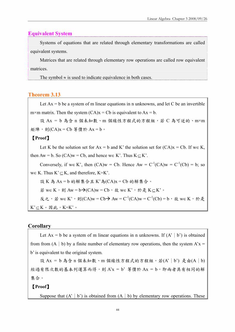
Linear Algebra- Chapter 3 20080926
44
Equivalent System Systems of equations that are related through elementary transformations are called
equivalent systems
Matrices that are related through elementary row operations are called row equivalent
matrices
The symbol asymp is used to indicate equivalence in both cases
Theorem 313 Let Ax = b be a system of m linear equations in n unknowns and let C be an invertible
mtimesm matrix Then the system (CA)x = Cb is equivalent to Ax = b
設 Ax = b 為含 n 個未知數m 個線性方程式的方程組若 C 為可逆的mtimesm
矩陣則(CA)x = Cb 等價於 Ax = b
【Proof】
Let K be the solution set for Ax = b and Krsquo the solution set for (CA)x = Cb If wisinK
then Aw = b So (CA)w = Cb and hence wisinKrsquo Thus KsubeKrsquo
Conversely if wisinKrsquo then (CA)w = Cb Hence Aw = C-1(CA)w = C-1(Cb) = b so
wisinK Thus KrsquosubeK and therefore K=Krsquo
設 K 為 Ax = b 的解集合且 Krsquo為(CA)x = Cb 的解集合
若 wisinK則 Aw = b (CA)w = Cb故 wisinKrsquo於是 KsubeKrsquo
反之若 wisinKrsquo則(CA)w = Cb Aw = C-1(CA)w = C-1(Cb) = b故 wisinK於是
KrsquosubeK因此K=Krsquo
Corollary Let Ax = b be a system of m linear equations in n unknowns If (Arsquo brsquo) is obtained ∣
from from (A b) by a finite number of elementary row operations then the system Arsquox = ∣
brsquo is equivalent to the original system
設 Ax = b 為含 n 個未知數m 個線性方程式的方程組若(Arsquo brsquo) ∣ 是由(A b) ∣
經過有限次數的基本列運算而得則 Arsquox = brsquo 等價於 Ax = b即兩者具有相同的解
集合
【Proof】
Suppose that (Arsquo brsquo) is obtained from (A b) by elementary row operations These ∣ ∣
Linear Algebra- Chapter 3 20080926
45
may be executed by multiplying (A b) by elementary mtimesm matrices E∣ 1 E2hellipEp Let
C=EphellipE2E1 then (Arsquo brsquo) = C(A b) = (CA Cb)∣ ∣ ∣
Since each Ei is invertible so is C Now Arsquo = CA and brsquo = Cb Thus by Theorem 313
the system Arsquox = brsquo is equivalent to the system Ax = b
設(Arsquo brsquo)∣ 是由(A b)∣ 經過基本列運算取得即以基本 mtimesm 矩陣 E1 E2hellipEp
乘上 (A b)∣ (Arsquo brsquo) = C(A b) = (CA Cb∣ ∣ ∣ )其中C=EphellipE2E1
因 Ei 可逆故 C 亦為可逆 Arsquo = CA 且 brsquo = Cb
依據 Theorem 313Arsquox = brsquo 等價於 Ax = b
Theorem 313 Let Ax = b be a system of m linear equations in n unknowns and let C be an
invertible mtimesm matrix Then the system (CA)x = Cb is equivalent to Ax = b 設 Ax = b
為含 n 個未知數m 個線性方程式的方程組若 C 為可逆的mtimesm 矩陣則(CA)x
= Cb 等價於 Ax = b
We now describe a method for solving any stystem of linear equations Consider for
example the system of linear equations
探討解線性方程組的方法hellip
2xxx2x3xxx1x2x3x2x3
4321
321
4321
=minus++=++=minus++
First we form the augmented matrix ⎟⎟⎟
⎠
⎞
⎜⎜⎜
⎝
⎛
minus
minus
231
112101112323
(增廣矩陣)
Interchanging the first and third rows ⎟⎟⎟
⎠
⎞
⎜⎜⎜
⎝
⎛
minus
minus
132
132301111121
(第 13 列互調)
Adding -1 times the first row to the second row and then add -3 times the first row to
the third row ⎟⎟⎟
⎠
⎞
⎜⎜⎜
⎝
⎛
minusminusminus
minus
512
104010101121
(第 1 列乘上 -1 加到第 2 列再以 -3 乘上
第 1 列加到第 3 列)
Linear Algebra- Chapter 3 20080926
46
Multiplying the second row by -1 ⎟⎟⎟
⎠
⎞
⎜⎜⎜
⎝
⎛
minusminus
minusminusminus
51
2
104010101121
(第 2 列乘上 -1)
Adding four times the second row to the third row ⎟⎟⎟
⎠
⎞
⎜⎜⎜
⎝
⎛
minusminus
minusminusminus
91
2
300010101121
(4 乘上第 2
列加到第 3 列)
Multiplying the third row by -13 ⎟⎟⎟
⎠
⎞
⎜⎜⎜
⎝
⎛minusminus
minus
31
2
100010101121
(第 3 列乘上 -13)
Adding the third row to the first and second rows to obtain zeros in row 1 column 4
and row 2 column 4 ⎟⎟⎟
⎠
⎞
⎜⎜⎜
⎝
⎛
325
100000100121
(將第 3 列加到第 1 列及第 2 列)
Adding -2 times the second row to the first row in order to make the first row second
column entry become zero ⎟⎟⎟
⎠
⎞
⎜⎜⎜
⎝
⎛
321
100000100101
(將第 2 列乘以 -2 再加至第 1 列)
We have now obtained the desired reduction of the augmented matrix
⎟⎟⎟
⎠
⎞
⎜⎜⎜
⎝
⎛
321
100000100101
是化簡後的增廣矩陣
This matrix corresponds to the system of linear equations
對應的線性方程組為
2x3x1xx
4
2
31
===+
By Corollary to Theorem 313 this system is equivalent to the original system But this
system is easily solved Obviously x2 = 2 and x4 = 3 Moreover x1 and x3 can be any values
Linear Algebra- Chapter 3 20080926
47
provided their sum is 1 Letting x3 = t we then have x1 = 1 ndash t Thus an arbitray solution to the
original system has the form
依據 Corollary to Theorem 313 化簡後的方程組與原方程組等值此方程組的解為
x2 = 3x4 = 3x1 + x3 = 1於是原方程組的任意解可以寫成
⎟⎟⎟⎟⎟
⎠
⎞
⎜⎜⎜⎜⎜
⎝
⎛minus
+
⎟⎟⎟⎟⎟
⎠
⎞
⎜⎜⎜⎜⎜
⎝
⎛
=
⎟⎟⎟⎟⎟
⎠
⎞
⎜⎜⎜⎜⎜
⎝
⎛ minus
0101
t
3021
3t2
t1
Observe that
⎪⎪⎭
⎪⎪⎬
⎫
⎪⎪⎩
⎪⎪⎨
⎧
⎟⎟⎟⎟⎟
⎠
⎞
⎜⎜⎜⎜⎜
⎝
⎛minus
0101
is a basis for the homogeneous system of equations
corresponding to the given system
其中
⎪⎪⎭
⎪⎪⎬
⎫
⎪⎪⎩
⎪⎪⎨
⎧
⎟⎟⎟⎟⎟
⎠
⎞
⎜⎜⎜⎜⎜
⎝
⎛minus
0101
是齊次方程組解集合的一組基底
Gauss-Jordan Elimination
Let A be an n times n matrix
1 Adjoin the identity n times n matrix In to A to form the matrix [A In]
2 Compute the reduced echelon form of [A In]
(1) If the reduced echelon form is of the type [In B] then B is the inverse of A
(2) If the reduced echelon form is not of the type [In B] in that the first n times n
submatrix is not In then A has no inverse
An n times n matrix A is invertible if and only if its reduced echelon form is In
DEFINITION 37 Reduced Row Echelon Form
A matrix is said to be in reduced row echelon form if the following three conditions
are satisfied
Linear Algebra- Chapter 3 20080926
48
一個矩陣可以被稱為簡約列梯形式必須具備有下列三條件
(a) Any row containing a nonzero entry preceeds any row in which all the entries are
zero (if any)
含有非零元素的任一列排在全含零元素的任一列前面(儘可能)
(b) The first nonzero entry in each row in the only nonzero entry in its column
各列中第一個非零元素為其所在行中唯一的非零元素
(c) The first nonzero entry in each row is 1 and it occurs in a column to thr right of the
first nonzero entry in the preceeding row
各列中第一個非零元素為 1 且它出現在前一列中第一個非零元素的右邊某一
行中
Reduced Echelon Form A matrix is in reduced echelon form if
1 Any rows consisting entirely of zeros are grouped at the bottom of the matrix
2 The first nonzero element of each other row is 1 This element is called a leading 1
3 The leading 1 of each row after the first is positioned to the right of the leading 1 of
the previous row
4 All other elements in a column that contains a leading 1 are zero
Theorem 314 Gaussian Elimination Transformation Gaussian elimination transform any matrix into its reduced row echelon form
利用 Gaussian elimination 將矩陣轉換成簡約列梯形式
We now describe a method for solving a system in which the augmented matrix is in
reduced row echelon form To illustrate this procedure we consider the system
14x8x3x2x2x28x5x2xxx6x3xxxx17x9x4xx3x2
54321
54321
54321
54321
=minus+++=minus+++=minus+++=minus+++
Linear Algebra- Chapter 3 20080926
49
for which the augmented matrix is
⎟⎟⎟⎟⎟
⎠
⎞
⎜⎜⎜⎜⎜
⎝
⎛
minusminusminusminus
1486
17
83222521113111194132
(增廣矩陣)
Applying Gaussian elimination to the augmented matrix of the system produces the
following sequence of matrices
利用 Gaussian elimination method 處理增廣矩陣
⎟⎟⎟⎟⎟
⎠
⎞
⎜⎜⎜⎜⎜
⎝
⎛
minusminusminusminus
1486
17
83222521113111194132
⎟⎟⎟⎟⎟
⎠
⎞
⎜⎜⎜⎜⎜
⎝
⎛
minusminusminusminus
148
176
83222521119413231111
⎟⎟⎟⎟⎟
⎠
⎞
⎜⎜⎜⎜⎜
⎝
⎛
minusminus
minus
0213
0000021000
1011020201
The system of linear equations corresponding to thus last matrix is
對應最後矩陣的線性方程組 2x2x
1xxx3x2x2x
54
532
531
=minus=+minus=minus+
Assign x3 = t1 x5 = t2
2t22x2x1tt1xxx
3t2t23x2x2x
254
21532
21531
+=+=+minus=+minus=
++minus=++minus=
Thus an arbitray solution s is of the form
於是任意解 s 具有下列形式
s =
⎟⎟⎟⎟⎟⎟
⎠
⎞
⎜⎜⎜⎜⎜⎜
⎝
⎛minus
+
⎟⎟⎟⎟⎟⎟
⎠
⎞
⎜⎜⎜⎜⎜⎜
⎝
⎛minus
+
⎟⎟⎟⎟⎟⎟
⎠
⎞
⎜⎜⎜⎜⎜⎜
⎝
⎛
=
⎟⎟⎟⎟⎟⎟
⎠
⎞
⎜⎜⎜⎜⎜⎜
⎝
⎛
+
+minus++minus
=
⎟⎟⎟⎟⎟⎟
⎠
⎞
⎜⎜⎜⎜⎜⎜
⎝
⎛
1201
2
t
00112
t
02013
t2t2
t1tt
3t2t2
xxxxx
21
2
2
1
21
21
5
4
3
2
1
where t1t2isinR
Linear Algebra- Chapter 3 20080926
50
Notice that
⎪⎪⎪
⎭
⎪⎪⎪
⎬
⎫
⎪⎪⎪
⎩
⎪⎪⎪
⎨
⎧
⎟⎟⎟⎟⎟⎟
⎠
⎞
⎜⎜⎜⎜⎜⎜
⎝
⎛minus
⎟⎟⎟⎟⎟⎟
⎠
⎞
⎜⎜⎜⎜⎜⎜
⎝
⎛minus
1201
2
00112
is a basis for the solution set of the corresponding
homogeneous system of equation and
⎟⎟⎟⎟⎟⎟
⎠
⎞
⎜⎜⎜⎜⎜⎜
⎝
⎛
02013
is a particular solution to the original system
⎪⎪⎪
⎭
⎪⎪⎪
⎬
⎫
⎪⎪⎪
⎩
⎪⎪⎪
⎨
⎧
⎟⎟⎟⎟⎟⎟
⎠
⎞
⎜⎜⎜⎜⎜⎜
⎝
⎛minus
⎟⎟⎟⎟⎟⎟
⎠
⎞
⎜⎜⎜⎜⎜⎜
⎝
⎛minus
1201
2
00112
是齊次方程組解集合的一組基底
⎟⎟⎟⎟⎟⎟
⎠
⎞
⎜⎜⎜⎜⎜⎜
⎝
⎛
02013
是原方程組的特別解
EXAMPLE 1
The matrix ⎟⎟⎟
⎠
⎞
⎜⎜⎜
⎝
⎛
101010011
is not in reduced row echelon form
因為第一行含有第一個非零元素在第一列但第一行尚含有其他非零元素
The matrix ⎟⎟⎟
⎠
⎞
⎜⎜⎜
⎝
⎛
110010012010
is not in reduced row echelon form
因為第一列第一個非零元素不在第一列第一個非零元素的右邊
The matrix ⎟⎟⎠
⎞⎜⎜⎝
⎛010002
is not in reduced row echelon form
因為第一列的第一個非零元素不是 1
Linear Algebra- Chapter 3 20080926
51
Reduced Echelon FormReduced Echelon Form
⎥⎥⎥
⎦
⎤
⎢⎢⎢
⎣
⎡
910030107001
⎥⎥⎥
⎦
⎤
⎢⎢⎢
⎣
⎡
100001000041
⎥⎥⎥
⎦
⎤
⎢⎢⎢
⎣
⎡
000210801
Not in Reduced Echelon Form
⎥⎥⎥
⎦
⎤
⎢⎢⎢
⎣
⎡
310000004021
⎥⎥⎥
⎦
⎤
⎢⎢⎢
⎣
⎡
100000430003021
⎥⎥⎥⎥
⎦
⎤
⎢⎢⎢⎢
⎣
⎡
0000210030108071
In Reduced Echelon Form
Use GaussUse Gauss--Jordan elimination to Jordan elimination to find reduced echelon formfind reduced echelon form 1313
Step 1 Interchange rows if necessary to bring a nonzero Step 1 Interchange rows if necessary to bring a nonzero element to the top of the first nonzero column This nonzero element to the top of the first nonzero column This nonzero element is called a pivotelement is called a pivot
⎥⎥⎦
⎤
⎢⎢⎣
⎡
minusminus
minus
1211244129333
22200
⎥⎥⎥
⎦
⎤
⎢⎢⎢
⎣
⎡
minusminus
minus
harrasymp
121124422200
129333
R2R1
Use GaussUse Gauss--Jordan elimination to Jordan elimination to find reduced echelon formfind reduced echelon form 2323
Step 2 Create a 1 in the pivot location by multiplying the Step 2 Create a 1 in the pivot location by multiplying the pivot row by 1pivotpivot row by 1pivot
Step 3 Create zero elsewhere in the pivot column by adding Step 3 Create zero elsewhere in the pivot column by adding suitable multiples of the pivot row to all other rows of the suitable multiples of the pivot row to all other rows of the matrixmatrix
⎥⎥⎥
⎦
⎤
⎢⎢⎢
⎣
⎡
minusminusminus
minus
minus+asymp
412002220043111
4)R1(R3
⎥⎥⎦
⎤
⎢⎢⎣
⎡
minusminus
minus
⎟⎠⎞
⎜⎝⎛asymp
12112442220043111
R13
1
The matrix is the reduced echelon form of the given matrixThe matrix is the reduced echelon form of the given matrix
Use GaussUse Gauss--Jordan elimination to Jordan elimination to find reduced echelon formfind reduced echelon form 3333
Step 4 Cover the pivot row and all rows above it Repeat Steps Step 4 Cover the pivot row and all rows above it Repeat Steps 1 1 and 2 for the remaining and 2 for the remaining submatrixsubmatrix Repeat Step 3 for the whole Repeat Step 3 for the whole matrix Continue until the reduced echelon form is reachedmatrix Continue until the reduced echelon form is reached
⎥⎥⎥
⎦
⎤
⎢⎢⎢
⎣
⎡
minusminus
+minus+asymp
⎥⎥⎥
⎦
⎤
⎢⎢⎢
⎣
⎡
minusminus
minus++asymp
⎥⎥⎥
⎦
⎤
⎢⎢⎢
⎣
⎡
minusminusminus
minus
⎟⎠⎞
⎜⎝⎛
asymp
⎥⎥⎥
⎦
⎤
⎢⎢⎢
⎣
⎡
minusminusminus
minus
6100050100
170011
R3R22)R3(R1
610001110052011
R2)2(R3R2R1
412001110043111
R221
412002220043111
Theorem 315 Let Ax = b be a system of r nonzero equations is in n unknown Suppose that rank(A)
= rank (A b)∣ and that (A b)∣ is in reduced row echelon form Then
設 Ax = b 為含有 n 個未知數r 個非零方程式的方程組假設 rank(A) = rank
(A b)∣ 且 (A b)∣ 為簡約列梯形式於是
(a) rank(A) = r
(b) If the general solution obtained by the procedure above is of the form s = s0 + t1u1
+ t2u2 +hellip+ tn-run-r then u1 u2hellip un-r is a basis for the solution set of the
corresponding homogeneous system and s0 is a solution to the original system 由
前述方法所得的 General solution 具有下列形式
s = s0 + t1u1 + t2u2 +hellip+ tn-run-r
其中u1 u2hellip un-r為齊次方程組 Ax = 0 的解集合的一組基底且 s0 為原方
程組的一個解)
【Proof】
Since (A b)∣ is in reduced row echelon form (A b)∣ must have r nonzero rows
Clearly these rows are linearly independent by the definition of the reduced row echelon
Linear Algebra- Chapter 3 20080926
52
form and so rank (A b)∣ = r Thus rank(A) = r
Let K be the solution set for Ax = b and let KH be the solution set for Ax = 0 Setting
t1 = t2 =hellip= tn-r = 0 we see that s = s0isinK But by Theorem 39 K = s +KH Hence
KH = - s0+K = span(u1 u2hellip un-r )
Because rank(A) = r we have dim(KH) = n-r Thus since dim(KH) = n-r and KH is
generated by a set u1 u2hellip un-r containing at most n-r vectors that is a basis for KH
由於(A b)∣ 具有簡約列梯形式因此(A b)∣ 必定具有 r 個非零列由簡約列梯形
式的定義得知 r 個非零列為線性獨立故 rank (A b)∣ = rrank(A) = r
令 K 為 Ax = b 的解集合 KH 為 Ax = 0 的解集合
假設 t1 = t2 =hellip= tn-r = 0(u1 u2hellip un-r非 KH的基底)則 s = s0isinK
依據 Theorem 39K = s +KH KH = - s0+K = span(u1 u2hellip un-r )
因 rank(A) = r所以 dim(KH) = n - r 且 KH 是由u1 u2hellip un-r 所生成
故原假設「t1 = t2 =hellip= tn-r = 0」不成立
因此 KH含有最多 n - r 個向量且這些向量為 KH的基底
Theorem 39 Let K be the solution set of a system of linear equations Ax = b and let KH be
the solution set of the corresponding homogeneous system Ax = 0 Then for any solution s
to Ax = b K =s + KH = s+k kisinKH 設 K 為線性方程組 Ax = b 的解集合且 KH
為對應的齊次方程組的解集合則對 Ax = b 的任一個解 s 而言K =s + KH = s+k
kisinKH
ExampleExampleSolve the system of equationsSolve the system of equations
7537429333
321
321
321
=minusminus=+minus=+minus
xxxxxxxxx
⎥⎥⎦
⎤
⎢⎢⎣
⎡
++asymp
000012104301
R2R3R2R1 12
431243
32
31
32
31+minus=+minus=rArr=+
=+rArr xxxx
xxxx
The general solution to the system isThe general solution to the system is
parameter) a (callednumber real is where 1243
3
2
1
rrxrxrx
=+minus=+minus=
⎥⎥⎥
⎦
⎤
⎢⎢⎢
⎣
⎡
minusminusminus
minus
minus+minus+asymp
⎥⎥⎥
⎦
⎤
⎢⎢⎢
⎣
⎡
minusminusminusminus
asymp
⎥⎥⎥
⎦
⎤
⎢⎢⎢
⎣
⎡
minusminusminusminus
242012103111
1R)3(3R1R)2(2R
715374123111
715374129333
R131
ExampleExample
Solve the system of equationsSolve the system of equations446942
1423258101242
4321
4321
4321
=minus+minusminus=+minus+minus
=minus+minus
xxxxxxxxxxxx
⎪⎪
⎩
⎪⎪
⎨
⎧
===
minus=
rArr==minus=minus
rArr
1x6xrx
2r2x
1x6x
2x2x
4
3
2
1
4
3
21
⎥⎥⎥
⎦
⎤
⎢⎢⎢
⎣
⎡ minusminusasymp
⎥⎥⎥
⎦
⎤
⎢⎢⎢
⎣
⎡minus
minusminusasymp
⎥⎥⎥
⎦
⎤
⎢⎢⎢
⎣
⎡
minusminusminusminusminusasymp
⎥⎥⎥
⎦
⎤
⎢⎢⎢
⎣
⎡
minusminusminusminusminusasymp
⎥⎥⎥
⎦
⎤
⎢⎢⎢
⎣
⎡
minusminusminusminusminus
minusminusasymp
⎥⎥⎥
⎦
⎤
⎢⎢⎢
⎣
⎡
minusminusminusminusminus
minusminus
+
minus+
+
minus+
minus+
+
110006010020021
110005110011021
14430051100
295621
2R31
144300153300295621
446942142321295621
44694214232158101242
R3R2
1)R3(R1
3R2R3
6)R2(R1
2)R1(R3
R1R2R1
21
Linear Algebra- Chapter 3 20080926
53
ExampleExampleSolve the system of equationsSolve the system of equations
432636242232
54321
54321
54321
=+minus+minusminus=++minus+=++minus+
xxxxxxxxxxxxxxx
⎥⎥⎦
⎤
⎢⎢⎣
⎡ minusasymp
⎥⎥⎦
⎤
⎢⎢⎣
⎡
minusminusminusminusminus
+
minus+
642000210000213121
431121636242213121
R1R3
2)R1(R2
⎥⎥⎦
⎤
⎢⎢⎣
⎡ minusasympharr 210000
642000213121
R3R2 ( ) ⎥⎥⎦
⎤
⎢⎢⎣
⎡ minusasymp
210000321000213121
2R21
⎥⎥⎦
⎤
⎢⎢⎣
⎡ minusminusminusasympminus+ 210000
321000750121
3)R2(R1 ⎥⎥⎦
⎤
⎢⎢⎣
⎡minus
minusasymp
minus+
+
210000101000300121
2)R3(R2
5R3R1
2x1x
3xx2x
5
4
321
=minus=
++minus=rArr
2xs and r somefor 1x sx rx
3sr2x
5
432
1
=minus===
++minus=
ExampleExample
Solve the system of Solve the system of equationsequations 122
32452232
32
321
321
321
=+minus=minus+
=+minus=+minus
xxxxxxxxxxx
⎥⎥
⎦
⎤
⎢⎢
⎣
⎡asymp
minusminusminus
minus
harr1220210063303211
R3R2
( ) ⎥⎥
⎦
⎤
⎢⎢
⎣
⎡asymp
minusminusminus
minus
1220210021103211
R231
⎥⎥
⎦
⎤
⎢⎢
⎣
⎡asympminusminusminus
minus+
+
5400210021101101
2)R2(R4
R2R1 ⎥⎥
⎦
⎤
⎢⎢
⎣
⎡asymp
minusminus
minus+
+
minus+
13000210040103001
4)R3R(R4
R3R2
1)R3(R1
( ) ⎥⎥
⎦
⎤
⎢⎢
⎣
⎡asymp
minusminus
1000210040103001
R4131
The system has no solutionThe system has no solution
⎥⎥
⎦
⎤
⎢⎢
⎣
⎡asymp
⎥⎥
⎦
⎤
⎢⎢
⎣
⎡
minusminusminus
minus
minusminusminusminus
minus+
minus+
1220633021003211
1220312145223211
1)R1(R3
2)R1(R2
0x1+0x2+0x3=1
Curve FittingCurve Fitting
A set of data points A set of data points is given and it is is given and it is necessary to find a polynomial whose graph passes through the necessary to find a polynomial whose graph passes through the points points The points are often measurements in an experiment The points are often measurements in an experiment The xThe x--coordinates are called coordinates are called base pointsbase pointsIt can be shown that if the base points are all distinct then aIt can be shown that if the base points are all distinct then a unique unique polynomial of degree n polynomial of degree n ndashndash 1 (or less)1 (or less)
can be fitted to thecan be fitted to the pointspoints
) ( ) ( ) ( 2211 nn yxyxyx K
11
2210
minusminus
minusminus ++++= n
nn
n xaxaxaay K
The coefficients can be found by substituting the points The coefficients can be found by substituting the points into the polynomial equation and then solving a system into the polynomial equation and then solving a system of linear equationsof linear equations
ExampleExample
Determine the equation of the polynomial of degree 2 whose graphpasses through the points (1 6) (2 3) (3 2)
Let the polynomial be and substituting x = 1 y = 6 x = 2 y = 3 x = 3 y = 2 we have
Solving this system for a0 a1 and a2 using Gauss-Jordan elimination
⎥⎥⎥
⎦
⎤
⎢⎢⎢
⎣
⎡minus
minus
minus+minus+asymp
220033109201
1)R2(R31)R2(R1
2210 xaxaay ++=
2a9a3a3a4a2a6aaa
210
210
210
=++=++=++
⎥⎥⎥
⎦
⎤
⎢⎢⎢
⎣
⎡
minusminus
⎥⎥⎥
⎦
⎤
⎢⎢⎢
⎣
⎡
minus+minus+asymp
482033106111
293134216111
1)R1(R31)R1(R2
( )⎥⎥⎥
⎦
⎤
⎢⎢⎢
⎣
⎡minus
⎥⎥⎥
⎦
⎤
⎢⎢⎢
⎣
⎡minus
minusasymp
minus++asymp
11006010
11001
110033109201
3)R3(R22R3R1
R321
We get a0 = 11 a1 = ndash 6 a2 = 1The parabola that passes through these points is y = 11 ndash 6x + x2
ExampleExample Traffic FlowTraffic Flow
Network analysis plays an important role in electrical Network analysis plays an important role in electrical engineeringengineeringThe concepts and tools of network analysis have been The concepts and tools of network analysis have been found to be useful in many other fields such as found to be useful in many other fields such as information theory and the study of transportation systemsinformation theory and the study of transportation systemsThe analysis of traffic flow through a road network during The analysis of traffic flow through a road network during peak period illustrates how systems of linear equations peak period illustrates how systems of linear equations with with manymany solutions can arise in practicesolutions can arise in practice
Traffic FlowTraffic Flow
Consider the typical road network The streets are all oneConsider the typical road network The streets are all one--way with the arrows indicating the direction of traffic flowway with the arrows indicating the direction of traffic flowThe flow of traffic in and out of the network is measured The flow of traffic in and out of the network is measured in vehicles per hour (in vehicles per hour (vphvph))How to construct a mathematical model to analyze this How to construct a mathematical model to analyze this network network
Traffic Traffic FlowFlowTRAFFIC LAWTRAFFIC LAWhelliphellipAll traffic entering an intersection must leave that All traffic entering an intersection must leave that intersectionintersection
Linear Algebra- Chapter 3 20080926
54
Junction AJunction BJunction CJunction DJunction EJunction F 600
800 200 500 100 600
54
643
73
72
621
51
=+=++minus=+minus=minus=+minus=+
xxxxx
xxxx
xxxxx
⎥⎥⎥⎥⎥⎥⎥⎥⎥⎥⎥⎥⎥
⎦
⎤
⎢⎢⎢⎢⎢⎢⎢⎢⎢⎢⎢⎢⎢
⎣
⎡
asympasymp
⎥⎥⎥⎥⎥⎥⎥⎥⎥⎥⎥⎥⎥
⎦
⎤
⎢⎢⎢⎢⎢⎢⎢⎢⎢⎢⎢⎢⎢
⎣
⎡
minusminus
minusminusminusminus
minusminus
minusminus
0000000001110000
6001101000200100010050010000106001100001
600001100080001011002001000100500100001010001000116000010001
L
Traffic FlowTraffic FlowJunction AJunction BJunction CJunction DJunction EJunction F 600
800 200 500 100 600
54
643
73
72
621
51
=+=++minus=+minus=minus=+minus=+
xxxxx
xxxx
xxxxx
Perform road work on x7 Because x3 ge 0 the minimum flow 200 in the branch x7 can be obtained by making x3 = 0 (closing DE to traffic)
Traffic FlowTraffic Flow
We get
765
76473
72761
xx x600xxx200x x500x x600xxx
minus=++minus=minus=+=+minusminus=
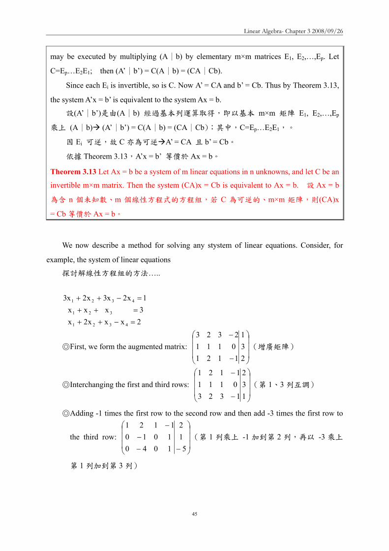
Linear Algebra- Chapter 3 20080926
47
provided their sum is 1 Letting x3 = t we then have x1 = 1 ndash t Thus an arbitray solution to the
original system has the form
依據 Corollary to Theorem 313 化簡後的方程組與原方程組等值此方程組的解為
x2 = 3x4 = 3x1 + x3 = 1於是原方程組的任意解可以寫成
⎟⎟⎟⎟⎟
⎠
⎞
⎜⎜⎜⎜⎜
⎝
⎛minus
+
⎟⎟⎟⎟⎟
⎠
⎞
⎜⎜⎜⎜⎜
⎝
⎛
=
⎟⎟⎟⎟⎟
⎠
⎞
⎜⎜⎜⎜⎜
⎝
⎛ minus
0101
t
3021
3t2
t1
Observe that
⎪⎪⎭
⎪⎪⎬
⎫
⎪⎪⎩
⎪⎪⎨
⎧
⎟⎟⎟⎟⎟
⎠
⎞
⎜⎜⎜⎜⎜
⎝
⎛minus
0101
is a basis for the homogeneous system of equations
corresponding to the given system
其中
⎪⎪⎭
⎪⎪⎬
⎫
⎪⎪⎩
⎪⎪⎨
⎧
⎟⎟⎟⎟⎟
⎠
⎞
⎜⎜⎜⎜⎜
⎝
⎛minus
0101
是齊次方程組解集合的一組基底
Gauss-Jordan Elimination
Let A be an n times n matrix
1 Adjoin the identity n times n matrix In to A to form the matrix [A In]
2 Compute the reduced echelon form of [A In]
(1) If the reduced echelon form is of the type [In B] then B is the inverse of A
(2) If the reduced echelon form is not of the type [In B] in that the first n times n
submatrix is not In then A has no inverse
An n times n matrix A is invertible if and only if its reduced echelon form is In
DEFINITION 37 Reduced Row Echelon Form
A matrix is said to be in reduced row echelon form if the following three conditions
are satisfied
Linear Algebra- Chapter 3 20080926
48
一個矩陣可以被稱為簡約列梯形式必須具備有下列三條件
(a) Any row containing a nonzero entry preceeds any row in which all the entries are
zero (if any)
含有非零元素的任一列排在全含零元素的任一列前面(儘可能)
(b) The first nonzero entry in each row in the only nonzero entry in its column
各列中第一個非零元素為其所在行中唯一的非零元素
(c) The first nonzero entry in each row is 1 and it occurs in a column to thr right of the
first nonzero entry in the preceeding row
各列中第一個非零元素為 1 且它出現在前一列中第一個非零元素的右邊某一
行中
Reduced Echelon Form A matrix is in reduced echelon form if
1 Any rows consisting entirely of zeros are grouped at the bottom of the matrix
2 The first nonzero element of each other row is 1 This element is called a leading 1
3 The leading 1 of each row after the first is positioned to the right of the leading 1 of
the previous row
4 All other elements in a column that contains a leading 1 are zero
Theorem 314 Gaussian Elimination Transformation Gaussian elimination transform any matrix into its reduced row echelon form
利用 Gaussian elimination 將矩陣轉換成簡約列梯形式
We now describe a method for solving a system in which the augmented matrix is in
reduced row echelon form To illustrate this procedure we consider the system
14x8x3x2x2x28x5x2xxx6x3xxxx17x9x4xx3x2
54321
54321
54321
54321
=minus+++=minus+++=minus+++=minus+++
Linear Algebra- Chapter 3 20080926
49
for which the augmented matrix is
⎟⎟⎟⎟⎟
⎠
⎞
⎜⎜⎜⎜⎜
⎝
⎛
minusminusminusminus
1486
17
83222521113111194132
(增廣矩陣)
Applying Gaussian elimination to the augmented matrix of the system produces the
following sequence of matrices
利用 Gaussian elimination method 處理增廣矩陣
⎟⎟⎟⎟⎟
⎠
⎞
⎜⎜⎜⎜⎜
⎝
⎛
minusminusminusminus
1486
17
83222521113111194132
⎟⎟⎟⎟⎟
⎠
⎞
⎜⎜⎜⎜⎜
⎝
⎛
minusminusminusminus
148
176
83222521119413231111
⎟⎟⎟⎟⎟
⎠
⎞
⎜⎜⎜⎜⎜
⎝
⎛
minusminus
minus
0213
0000021000
1011020201
The system of linear equations corresponding to thus last matrix is
對應最後矩陣的線性方程組 2x2x
1xxx3x2x2x
54
532
531
=minus=+minus=minus+
Assign x3 = t1 x5 = t2
2t22x2x1tt1xxx
3t2t23x2x2x
254
21532
21531
+=+=+minus=+minus=
++minus=++minus=
Thus an arbitray solution s is of the form
於是任意解 s 具有下列形式
s =
⎟⎟⎟⎟⎟⎟
⎠
⎞
⎜⎜⎜⎜⎜⎜
⎝
⎛minus
+
⎟⎟⎟⎟⎟⎟
⎠
⎞
⎜⎜⎜⎜⎜⎜
⎝
⎛minus
+
⎟⎟⎟⎟⎟⎟
⎠
⎞
⎜⎜⎜⎜⎜⎜
⎝
⎛
=
⎟⎟⎟⎟⎟⎟
⎠
⎞
⎜⎜⎜⎜⎜⎜
⎝
⎛
+
+minus++minus
=
⎟⎟⎟⎟⎟⎟
⎠
⎞
⎜⎜⎜⎜⎜⎜
⎝
⎛
1201
2
t
00112
t
02013
t2t2
t1tt
3t2t2
xxxxx
21
2
2
1
21
21
5
4
3
2
1
where t1t2isinR
Linear Algebra- Chapter 3 20080926
50
Notice that
⎪⎪⎪
⎭
⎪⎪⎪
⎬
⎫
⎪⎪⎪
⎩
⎪⎪⎪
⎨
⎧
⎟⎟⎟⎟⎟⎟
⎠
⎞
⎜⎜⎜⎜⎜⎜
⎝
⎛minus
⎟⎟⎟⎟⎟⎟
⎠
⎞
⎜⎜⎜⎜⎜⎜
⎝
⎛minus
1201
2
00112
is a basis for the solution set of the corresponding
homogeneous system of equation and
⎟⎟⎟⎟⎟⎟
⎠
⎞
⎜⎜⎜⎜⎜⎜
⎝
⎛
02013
is a particular solution to the original system
⎪⎪⎪
⎭
⎪⎪⎪
⎬
⎫
⎪⎪⎪
⎩
⎪⎪⎪
⎨
⎧
⎟⎟⎟⎟⎟⎟
⎠
⎞
⎜⎜⎜⎜⎜⎜
⎝
⎛minus
⎟⎟⎟⎟⎟⎟
⎠
⎞
⎜⎜⎜⎜⎜⎜
⎝
⎛minus
1201
2
00112
是齊次方程組解集合的一組基底
⎟⎟⎟⎟⎟⎟
⎠
⎞
⎜⎜⎜⎜⎜⎜
⎝
⎛
02013
是原方程組的特別解
EXAMPLE 1
The matrix ⎟⎟⎟
⎠
⎞
⎜⎜⎜
⎝
⎛
101010011
is not in reduced row echelon form
因為第一行含有第一個非零元素在第一列但第一行尚含有其他非零元素
The matrix ⎟⎟⎟
⎠
⎞
⎜⎜⎜
⎝
⎛
110010012010
is not in reduced row echelon form
因為第一列第一個非零元素不在第一列第一個非零元素的右邊
The matrix ⎟⎟⎠
⎞⎜⎜⎝
⎛010002
is not in reduced row echelon form
因為第一列的第一個非零元素不是 1
Linear Algebra- Chapter 3 20080926
51
Reduced Echelon FormReduced Echelon Form
⎥⎥⎥
⎦
⎤
⎢⎢⎢
⎣
⎡
910030107001
⎥⎥⎥
⎦
⎤
⎢⎢⎢
⎣
⎡
100001000041
⎥⎥⎥
⎦
⎤
⎢⎢⎢
⎣
⎡
000210801
Not in Reduced Echelon Form
⎥⎥⎥
⎦
⎤
⎢⎢⎢
⎣
⎡
310000004021
⎥⎥⎥
⎦
⎤
⎢⎢⎢
⎣
⎡
100000430003021
⎥⎥⎥⎥
⎦
⎤
⎢⎢⎢⎢
⎣
⎡
0000210030108071
In Reduced Echelon Form
Use GaussUse Gauss--Jordan elimination to Jordan elimination to find reduced echelon formfind reduced echelon form 1313
Step 1 Interchange rows if necessary to bring a nonzero Step 1 Interchange rows if necessary to bring a nonzero element to the top of the first nonzero column This nonzero element to the top of the first nonzero column This nonzero element is called a pivotelement is called a pivot
⎥⎥⎦
⎤
⎢⎢⎣
⎡
minusminus
minus
1211244129333
22200
⎥⎥⎥
⎦
⎤
⎢⎢⎢
⎣
⎡
minusminus
minus
harrasymp
121124422200
129333
R2R1
Use GaussUse Gauss--Jordan elimination to Jordan elimination to find reduced echelon formfind reduced echelon form 2323
Step 2 Create a 1 in the pivot location by multiplying the Step 2 Create a 1 in the pivot location by multiplying the pivot row by 1pivotpivot row by 1pivot
Step 3 Create zero elsewhere in the pivot column by adding Step 3 Create zero elsewhere in the pivot column by adding suitable multiples of the pivot row to all other rows of the suitable multiples of the pivot row to all other rows of the matrixmatrix
⎥⎥⎥
⎦
⎤
⎢⎢⎢
⎣
⎡
minusminusminus
minus
minus+asymp
412002220043111
4)R1(R3
⎥⎥⎦
⎤
⎢⎢⎣
⎡
minusminus
minus
⎟⎠⎞
⎜⎝⎛asymp
12112442220043111
R13
1
The matrix is the reduced echelon form of the given matrixThe matrix is the reduced echelon form of the given matrix
Use GaussUse Gauss--Jordan elimination to Jordan elimination to find reduced echelon formfind reduced echelon form 3333
Step 4 Cover the pivot row and all rows above it Repeat Steps Step 4 Cover the pivot row and all rows above it Repeat Steps 1 1 and 2 for the remaining and 2 for the remaining submatrixsubmatrix Repeat Step 3 for the whole Repeat Step 3 for the whole matrix Continue until the reduced echelon form is reachedmatrix Continue until the reduced echelon form is reached
⎥⎥⎥
⎦
⎤
⎢⎢⎢
⎣
⎡
minusminus
+minus+asymp
⎥⎥⎥
⎦
⎤
⎢⎢⎢
⎣
⎡
minusminus
minus++asymp
⎥⎥⎥
⎦
⎤
⎢⎢⎢
⎣
⎡
minusminusminus
minus
⎟⎠⎞
⎜⎝⎛
asymp
⎥⎥⎥
⎦
⎤
⎢⎢⎢
⎣
⎡
minusminusminus
minus
6100050100
170011
R3R22)R3(R1
610001110052011
R2)2(R3R2R1
412001110043111
R221
412002220043111
Theorem 315 Let Ax = b be a system of r nonzero equations is in n unknown Suppose that rank(A)
= rank (A b)∣ and that (A b)∣ is in reduced row echelon form Then
設 Ax = b 為含有 n 個未知數r 個非零方程式的方程組假設 rank(A) = rank
(A b)∣ 且 (A b)∣ 為簡約列梯形式於是
(a) rank(A) = r
(b) If the general solution obtained by the procedure above is of the form s = s0 + t1u1
+ t2u2 +hellip+ tn-run-r then u1 u2hellip un-r is a basis for the solution set of the
corresponding homogeneous system and s0 is a solution to the original system 由
前述方法所得的 General solution 具有下列形式
s = s0 + t1u1 + t2u2 +hellip+ tn-run-r
其中u1 u2hellip un-r為齊次方程組 Ax = 0 的解集合的一組基底且 s0 為原方
程組的一個解)
【Proof】
Since (A b)∣ is in reduced row echelon form (A b)∣ must have r nonzero rows
Clearly these rows are linearly independent by the definition of the reduced row echelon
Linear Algebra- Chapter 3 20080926
52
form and so rank (A b)∣ = r Thus rank(A) = r
Let K be the solution set for Ax = b and let KH be the solution set for Ax = 0 Setting
t1 = t2 =hellip= tn-r = 0 we see that s = s0isinK But by Theorem 39 K = s +KH Hence
KH = - s0+K = span(u1 u2hellip un-r )
Because rank(A) = r we have dim(KH) = n-r Thus since dim(KH) = n-r and KH is
generated by a set u1 u2hellip un-r containing at most n-r vectors that is a basis for KH
由於(A b)∣ 具有簡約列梯形式因此(A b)∣ 必定具有 r 個非零列由簡約列梯形
式的定義得知 r 個非零列為線性獨立故 rank (A b)∣ = rrank(A) = r
令 K 為 Ax = b 的解集合 KH 為 Ax = 0 的解集合
假設 t1 = t2 =hellip= tn-r = 0(u1 u2hellip un-r非 KH的基底)則 s = s0isinK
依據 Theorem 39K = s +KH KH = - s0+K = span(u1 u2hellip un-r )
因 rank(A) = r所以 dim(KH) = n - r 且 KH 是由u1 u2hellip un-r 所生成
故原假設「t1 = t2 =hellip= tn-r = 0」不成立
因此 KH含有最多 n - r 個向量且這些向量為 KH的基底
Theorem 39 Let K be the solution set of a system of linear equations Ax = b and let KH be
the solution set of the corresponding homogeneous system Ax = 0 Then for any solution s
to Ax = b K =s + KH = s+k kisinKH 設 K 為線性方程組 Ax = b 的解集合且 KH
為對應的齊次方程組的解集合則對 Ax = b 的任一個解 s 而言K =s + KH = s+k
kisinKH
ExampleExampleSolve the system of equationsSolve the system of equations
7537429333
321
321
321
=minusminus=+minus=+minus
xxxxxxxxx
⎥⎥⎦
⎤
⎢⎢⎣
⎡
++asymp
000012104301
R2R3R2R1 12
431243
32
31
32
31+minus=+minus=rArr=+
=+rArr xxxx
xxxx
The general solution to the system isThe general solution to the system is
parameter) a (callednumber real is where 1243
3
2
1
rrxrxrx
=+minus=+minus=
⎥⎥⎥
⎦
⎤
⎢⎢⎢
⎣
⎡
minusminusminus
minus
minus+minus+asymp
⎥⎥⎥
⎦
⎤
⎢⎢⎢
⎣
⎡
minusminusminusminus
asymp
⎥⎥⎥
⎦
⎤
⎢⎢⎢
⎣
⎡
minusminusminusminus
242012103111
1R)3(3R1R)2(2R
715374123111
715374129333
R131
ExampleExample
Solve the system of equationsSolve the system of equations446942
1423258101242
4321
4321
4321
=minus+minusminus=+minus+minus
=minus+minus
xxxxxxxxxxxx
⎪⎪
⎩
⎪⎪
⎨
⎧
===
minus=
rArr==minus=minus
rArr
1x6xrx
2r2x
1x6x
2x2x
4
3
2
1
4
3
21
⎥⎥⎥
⎦
⎤
⎢⎢⎢
⎣
⎡ minusminusasymp
⎥⎥⎥
⎦
⎤
⎢⎢⎢
⎣
⎡minus
minusminusasymp
⎥⎥⎥
⎦
⎤
⎢⎢⎢
⎣
⎡
minusminusminusminusminusasymp
⎥⎥⎥
⎦
⎤
⎢⎢⎢
⎣
⎡
minusminusminusminusminusasymp
⎥⎥⎥
⎦
⎤
⎢⎢⎢
⎣
⎡
minusminusminusminusminus
minusminusasymp
⎥⎥⎥
⎦
⎤
⎢⎢⎢
⎣
⎡
minusminusminusminusminus
minusminus
+
minus+
+
minus+
minus+
+
110006010020021
110005110011021
14430051100
295621
2R31
144300153300295621
446942142321295621
44694214232158101242
R3R2
1)R3(R1
3R2R3
6)R2(R1
2)R1(R3
R1R2R1
21
Linear Algebra- Chapter 3 20080926
53
ExampleExampleSolve the system of equationsSolve the system of equations
432636242232
54321
54321
54321
=+minus+minusminus=++minus+=++minus+
xxxxxxxxxxxxxxx
⎥⎥⎦
⎤
⎢⎢⎣
⎡ minusasymp
⎥⎥⎦
⎤
⎢⎢⎣
⎡
minusminusminusminusminus
+
minus+
642000210000213121
431121636242213121
R1R3
2)R1(R2
⎥⎥⎦
⎤
⎢⎢⎣
⎡ minusasympharr 210000
642000213121
R3R2 ( ) ⎥⎥⎦
⎤
⎢⎢⎣
⎡ minusasymp
210000321000213121
2R21
⎥⎥⎦
⎤
⎢⎢⎣
⎡ minusminusminusasympminus+ 210000
321000750121
3)R2(R1 ⎥⎥⎦
⎤
⎢⎢⎣
⎡minus
minusasymp
minus+
+
210000101000300121
2)R3(R2
5R3R1
2x1x
3xx2x
5
4
321
=minus=
++minus=rArr
2xs and r somefor 1x sx rx
3sr2x
5
432
1
=minus===
++minus=
ExampleExample
Solve the system of Solve the system of equationsequations 122
32452232
32
321
321
321
=+minus=minus+
=+minus=+minus
xxxxxxxxxxx
⎥⎥
⎦
⎤
⎢⎢
⎣
⎡asymp
minusminusminus
minus
harr1220210063303211
R3R2
( ) ⎥⎥
⎦
⎤
⎢⎢
⎣
⎡asymp
minusminusminus
minus
1220210021103211
R231
⎥⎥
⎦
⎤
⎢⎢
⎣
⎡asympminusminusminus
minus+
+
5400210021101101
2)R2(R4
R2R1 ⎥⎥
⎦
⎤
⎢⎢
⎣
⎡asymp
minusminus
minus+
+
minus+
13000210040103001
4)R3R(R4
R3R2
1)R3(R1
( ) ⎥⎥
⎦
⎤
⎢⎢
⎣
⎡asymp
minusminus
1000210040103001
R4131
The system has no solutionThe system has no solution
⎥⎥
⎦
⎤
⎢⎢
⎣
⎡asymp
⎥⎥
⎦
⎤
⎢⎢
⎣
⎡
minusminusminus
minus
minusminusminusminus
minus+
minus+
1220633021003211
1220312145223211
1)R1(R3
2)R1(R2
0x1+0x2+0x3=1
Curve FittingCurve Fitting
A set of data points A set of data points is given and it is is given and it is necessary to find a polynomial whose graph passes through the necessary to find a polynomial whose graph passes through the points points The points are often measurements in an experiment The points are often measurements in an experiment The xThe x--coordinates are called coordinates are called base pointsbase pointsIt can be shown that if the base points are all distinct then aIt can be shown that if the base points are all distinct then a unique unique polynomial of degree n polynomial of degree n ndashndash 1 (or less)1 (or less)
can be fitted to thecan be fitted to the pointspoints
) ( ) ( ) ( 2211 nn yxyxyx K
11
2210
minusminus
minusminus ++++= n
nn
n xaxaxaay K
The coefficients can be found by substituting the points The coefficients can be found by substituting the points into the polynomial equation and then solving a system into the polynomial equation and then solving a system of linear equationsof linear equations
ExampleExample
Determine the equation of the polynomial of degree 2 whose graphpasses through the points (1 6) (2 3) (3 2)
Let the polynomial be and substituting x = 1 y = 6 x = 2 y = 3 x = 3 y = 2 we have
Solving this system for a0 a1 and a2 using Gauss-Jordan elimination
⎥⎥⎥
⎦
⎤
⎢⎢⎢
⎣
⎡minus
minus
minus+minus+asymp
220033109201
1)R2(R31)R2(R1
2210 xaxaay ++=
2a9a3a3a4a2a6aaa
210
210
210
=++=++=++
⎥⎥⎥
⎦
⎤
⎢⎢⎢
⎣
⎡
minusminus
⎥⎥⎥
⎦
⎤
⎢⎢⎢
⎣
⎡
minus+minus+asymp
482033106111
293134216111
1)R1(R31)R1(R2
( )⎥⎥⎥
⎦
⎤
⎢⎢⎢
⎣
⎡minus
⎥⎥⎥
⎦
⎤
⎢⎢⎢
⎣
⎡minus
minusasymp
minus++asymp
11006010
11001
110033109201
3)R3(R22R3R1
R321
We get a0 = 11 a1 = ndash 6 a2 = 1The parabola that passes through these points is y = 11 ndash 6x + x2
ExampleExample Traffic FlowTraffic Flow
Network analysis plays an important role in electrical Network analysis plays an important role in electrical engineeringengineeringThe concepts and tools of network analysis have been The concepts and tools of network analysis have been found to be useful in many other fields such as found to be useful in many other fields such as information theory and the study of transportation systemsinformation theory and the study of transportation systemsThe analysis of traffic flow through a road network during The analysis of traffic flow through a road network during peak period illustrates how systems of linear equations peak period illustrates how systems of linear equations with with manymany solutions can arise in practicesolutions can arise in practice
Traffic FlowTraffic Flow
Consider the typical road network The streets are all oneConsider the typical road network The streets are all one--way with the arrows indicating the direction of traffic flowway with the arrows indicating the direction of traffic flowThe flow of traffic in and out of the network is measured The flow of traffic in and out of the network is measured in vehicles per hour (in vehicles per hour (vphvph))How to construct a mathematical model to analyze this How to construct a mathematical model to analyze this network network
Traffic Traffic FlowFlowTRAFFIC LAWTRAFFIC LAWhelliphellipAll traffic entering an intersection must leave that All traffic entering an intersection must leave that intersectionintersection
Linear Algebra- Chapter 3 20080926
54
Junction AJunction BJunction CJunction DJunction EJunction F 600
800 200 500 100 600
54
643
73
72
621
51
=+=++minus=+minus=minus=+minus=+
xxxxx
xxxx
xxxxx
⎥⎥⎥⎥⎥⎥⎥⎥⎥⎥⎥⎥⎥
⎦
⎤
⎢⎢⎢⎢⎢⎢⎢⎢⎢⎢⎢⎢⎢
⎣
⎡
asympasymp
⎥⎥⎥⎥⎥⎥⎥⎥⎥⎥⎥⎥⎥
⎦
⎤
⎢⎢⎢⎢⎢⎢⎢⎢⎢⎢⎢⎢⎢
⎣
⎡
minusminus
minusminusminusminus
minusminus
minusminus
0000000001110000
6001101000200100010050010000106001100001
600001100080001011002001000100500100001010001000116000010001
L
Traffic FlowTraffic FlowJunction AJunction BJunction CJunction DJunction EJunction F 600
800 200 500 100 600
54
643
73
72
621
51
=+=++minus=+minus=minus=+minus=+
xxxxx
xxxx
xxxxx
Perform road work on x7 Because x3 ge 0 the minimum flow 200 in the branch x7 can be obtained by making x3 = 0 (closing DE to traffic)
Traffic FlowTraffic Flow
We get
765
76473
72761
xx x600xxx200x x500x x600xxx
minus=++minus=minus=+=+minusminus=
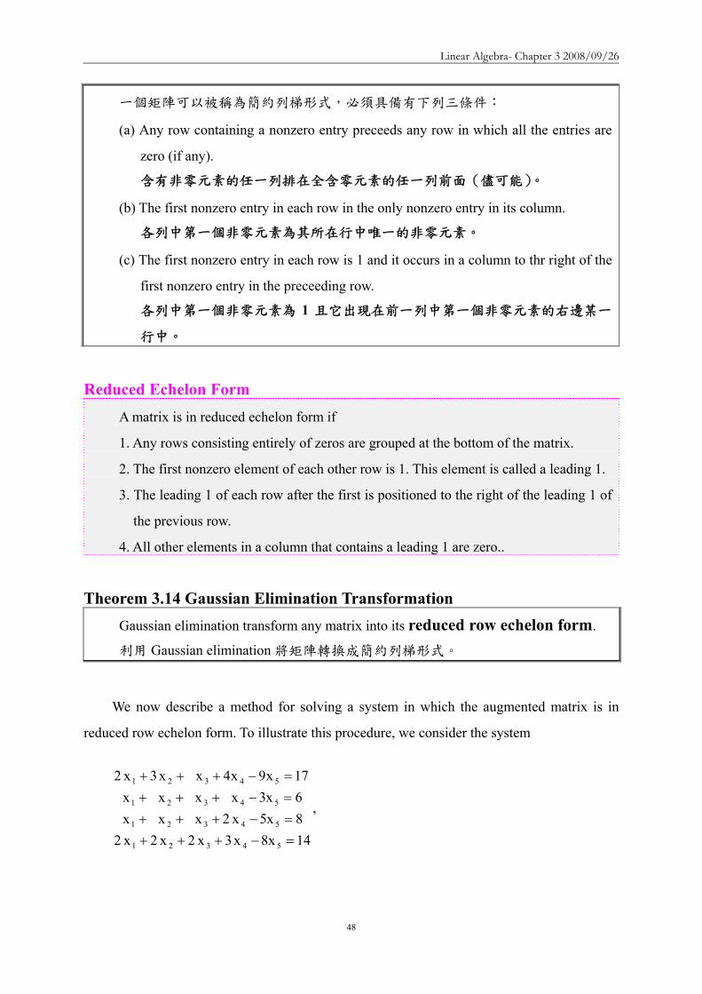
Linear Algebra- Chapter 3 20080926
48
一個矩陣可以被稱為簡約列梯形式必須具備有下列三條件
(a) Any row containing a nonzero entry preceeds any row in which all the entries are
zero (if any)
含有非零元素的任一列排在全含零元素的任一列前面(儘可能)
(b) The first nonzero entry in each row in the only nonzero entry in its column
各列中第一個非零元素為其所在行中唯一的非零元素
(c) The first nonzero entry in each row is 1 and it occurs in a column to thr right of the
first nonzero entry in the preceeding row
各列中第一個非零元素為 1 且它出現在前一列中第一個非零元素的右邊某一
行中
Reduced Echelon Form A matrix is in reduced echelon form if
1 Any rows consisting entirely of zeros are grouped at the bottom of the matrix
2 The first nonzero element of each other row is 1 This element is called a leading 1
3 The leading 1 of each row after the first is positioned to the right of the leading 1 of
the previous row
4 All other elements in a column that contains a leading 1 are zero
Theorem 314 Gaussian Elimination Transformation Gaussian elimination transform any matrix into its reduced row echelon form
利用 Gaussian elimination 將矩陣轉換成簡約列梯形式
We now describe a method for solving a system in which the augmented matrix is in
reduced row echelon form To illustrate this procedure we consider the system
14x8x3x2x2x28x5x2xxx6x3xxxx17x9x4xx3x2
54321
54321
54321
54321
=minus+++=minus+++=minus+++=minus+++
Linear Algebra- Chapter 3 20080926
49
for which the augmented matrix is
⎟⎟⎟⎟⎟
⎠
⎞
⎜⎜⎜⎜⎜
⎝
⎛
minusminusminusminus
1486
17
83222521113111194132
(增廣矩陣)
Applying Gaussian elimination to the augmented matrix of the system produces the
following sequence of matrices
利用 Gaussian elimination method 處理增廣矩陣
⎟⎟⎟⎟⎟
⎠
⎞
⎜⎜⎜⎜⎜
⎝
⎛
minusminusminusminus
1486
17
83222521113111194132
⎟⎟⎟⎟⎟
⎠
⎞
⎜⎜⎜⎜⎜
⎝
⎛
minusminusminusminus
148
176
83222521119413231111
⎟⎟⎟⎟⎟
⎠
⎞
⎜⎜⎜⎜⎜
⎝
⎛
minusminus
minus
0213
0000021000
1011020201
The system of linear equations corresponding to thus last matrix is
對應最後矩陣的線性方程組 2x2x
1xxx3x2x2x
54
532
531
=minus=+minus=minus+
Assign x3 = t1 x5 = t2
2t22x2x1tt1xxx
3t2t23x2x2x
254
21532
21531
+=+=+minus=+minus=
++minus=++minus=
Thus an arbitray solution s is of the form
於是任意解 s 具有下列形式
s =
⎟⎟⎟⎟⎟⎟
⎠
⎞
⎜⎜⎜⎜⎜⎜
⎝
⎛minus
+
⎟⎟⎟⎟⎟⎟
⎠
⎞
⎜⎜⎜⎜⎜⎜
⎝
⎛minus
+
⎟⎟⎟⎟⎟⎟
⎠
⎞
⎜⎜⎜⎜⎜⎜
⎝
⎛
=
⎟⎟⎟⎟⎟⎟
⎠
⎞
⎜⎜⎜⎜⎜⎜
⎝
⎛
+
+minus++minus
=
⎟⎟⎟⎟⎟⎟
⎠
⎞
⎜⎜⎜⎜⎜⎜
⎝
⎛
1201
2
t
00112
t
02013
t2t2
t1tt
3t2t2
xxxxx
21
2
2
1
21
21
5
4
3
2
1
where t1t2isinR
Linear Algebra- Chapter 3 20080926
50
Notice that
⎪⎪⎪
⎭
⎪⎪⎪
⎬
⎫
⎪⎪⎪
⎩
⎪⎪⎪
⎨
⎧
⎟⎟⎟⎟⎟⎟
⎠
⎞
⎜⎜⎜⎜⎜⎜
⎝
⎛minus
⎟⎟⎟⎟⎟⎟
⎠
⎞
⎜⎜⎜⎜⎜⎜
⎝
⎛minus
1201
2
00112
is a basis for the solution set of the corresponding
homogeneous system of equation and
⎟⎟⎟⎟⎟⎟
⎠
⎞
⎜⎜⎜⎜⎜⎜
⎝
⎛
02013
is a particular solution to the original system
⎪⎪⎪
⎭
⎪⎪⎪
⎬
⎫
⎪⎪⎪
⎩
⎪⎪⎪
⎨
⎧
⎟⎟⎟⎟⎟⎟
⎠
⎞
⎜⎜⎜⎜⎜⎜
⎝
⎛minus
⎟⎟⎟⎟⎟⎟
⎠
⎞
⎜⎜⎜⎜⎜⎜
⎝
⎛minus
1201
2
00112
是齊次方程組解集合的一組基底
⎟⎟⎟⎟⎟⎟
⎠
⎞
⎜⎜⎜⎜⎜⎜
⎝
⎛
02013
是原方程組的特別解
EXAMPLE 1
The matrix ⎟⎟⎟
⎠
⎞
⎜⎜⎜
⎝
⎛
101010011
is not in reduced row echelon form
因為第一行含有第一個非零元素在第一列但第一行尚含有其他非零元素
The matrix ⎟⎟⎟
⎠
⎞
⎜⎜⎜
⎝
⎛
110010012010
is not in reduced row echelon form
因為第一列第一個非零元素不在第一列第一個非零元素的右邊
The matrix ⎟⎟⎠
⎞⎜⎜⎝
⎛010002
is not in reduced row echelon form
因為第一列的第一個非零元素不是 1
Linear Algebra- Chapter 3 20080926
51
Reduced Echelon FormReduced Echelon Form
⎥⎥⎥
⎦
⎤
⎢⎢⎢
⎣
⎡
910030107001
⎥⎥⎥
⎦
⎤
⎢⎢⎢
⎣
⎡
100001000041
⎥⎥⎥
⎦
⎤
⎢⎢⎢
⎣
⎡
000210801
Not in Reduced Echelon Form
⎥⎥⎥
⎦
⎤
⎢⎢⎢
⎣
⎡
310000004021
⎥⎥⎥
⎦
⎤
⎢⎢⎢
⎣
⎡
100000430003021
⎥⎥⎥⎥
⎦
⎤
⎢⎢⎢⎢
⎣
⎡
0000210030108071
In Reduced Echelon Form
Use GaussUse Gauss--Jordan elimination to Jordan elimination to find reduced echelon formfind reduced echelon form 1313
Step 1 Interchange rows if necessary to bring a nonzero Step 1 Interchange rows if necessary to bring a nonzero element to the top of the first nonzero column This nonzero element to the top of the first nonzero column This nonzero element is called a pivotelement is called a pivot
⎥⎥⎦
⎤
⎢⎢⎣
⎡
minusminus
minus
1211244129333
22200
⎥⎥⎥
⎦
⎤
⎢⎢⎢
⎣
⎡
minusminus
minus
harrasymp
121124422200
129333
R2R1
Use GaussUse Gauss--Jordan elimination to Jordan elimination to find reduced echelon formfind reduced echelon form 2323
Step 2 Create a 1 in the pivot location by multiplying the Step 2 Create a 1 in the pivot location by multiplying the pivot row by 1pivotpivot row by 1pivot
Step 3 Create zero elsewhere in the pivot column by adding Step 3 Create zero elsewhere in the pivot column by adding suitable multiples of the pivot row to all other rows of the suitable multiples of the pivot row to all other rows of the matrixmatrix
⎥⎥⎥
⎦
⎤
⎢⎢⎢
⎣
⎡
minusminusminus
minus
minus+asymp
412002220043111
4)R1(R3
⎥⎥⎦
⎤
⎢⎢⎣
⎡
minusminus
minus
⎟⎠⎞
⎜⎝⎛asymp
12112442220043111
R13
1
The matrix is the reduced echelon form of the given matrixThe matrix is the reduced echelon form of the given matrix
Use GaussUse Gauss--Jordan elimination to Jordan elimination to find reduced echelon formfind reduced echelon form 3333
Step 4 Cover the pivot row and all rows above it Repeat Steps Step 4 Cover the pivot row and all rows above it Repeat Steps 1 1 and 2 for the remaining and 2 for the remaining submatrixsubmatrix Repeat Step 3 for the whole Repeat Step 3 for the whole matrix Continue until the reduced echelon form is reachedmatrix Continue until the reduced echelon form is reached
⎥⎥⎥
⎦
⎤
⎢⎢⎢
⎣
⎡
minusminus
+minus+asymp
⎥⎥⎥
⎦
⎤
⎢⎢⎢
⎣
⎡
minusminus
minus++asymp
⎥⎥⎥
⎦
⎤
⎢⎢⎢
⎣
⎡
minusminusminus
minus
⎟⎠⎞
⎜⎝⎛
asymp
⎥⎥⎥
⎦
⎤
⎢⎢⎢
⎣
⎡
minusminusminus
minus
6100050100
170011
R3R22)R3(R1
610001110052011
R2)2(R3R2R1
412001110043111
R221
412002220043111
Theorem 315 Let Ax = b be a system of r nonzero equations is in n unknown Suppose that rank(A)
= rank (A b)∣ and that (A b)∣ is in reduced row echelon form Then
設 Ax = b 為含有 n 個未知數r 個非零方程式的方程組假設 rank(A) = rank
(A b)∣ 且 (A b)∣ 為簡約列梯形式於是
(a) rank(A) = r
(b) If the general solution obtained by the procedure above is of the form s = s0 + t1u1
+ t2u2 +hellip+ tn-run-r then u1 u2hellip un-r is a basis for the solution set of the
corresponding homogeneous system and s0 is a solution to the original system 由
前述方法所得的 General solution 具有下列形式
s = s0 + t1u1 + t2u2 +hellip+ tn-run-r
其中u1 u2hellip un-r為齊次方程組 Ax = 0 的解集合的一組基底且 s0 為原方
程組的一個解)
【Proof】
Since (A b)∣ is in reduced row echelon form (A b)∣ must have r nonzero rows
Clearly these rows are linearly independent by the definition of the reduced row echelon
Linear Algebra- Chapter 3 20080926
52
form and so rank (A b)∣ = r Thus rank(A) = r
Let K be the solution set for Ax = b and let KH be the solution set for Ax = 0 Setting
t1 = t2 =hellip= tn-r = 0 we see that s = s0isinK But by Theorem 39 K = s +KH Hence
KH = - s0+K = span(u1 u2hellip un-r )
Because rank(A) = r we have dim(KH) = n-r Thus since dim(KH) = n-r and KH is
generated by a set u1 u2hellip un-r containing at most n-r vectors that is a basis for KH
由於(A b)∣ 具有簡約列梯形式因此(A b)∣ 必定具有 r 個非零列由簡約列梯形
式的定義得知 r 個非零列為線性獨立故 rank (A b)∣ = rrank(A) = r
令 K 為 Ax = b 的解集合 KH 為 Ax = 0 的解集合
假設 t1 = t2 =hellip= tn-r = 0(u1 u2hellip un-r非 KH的基底)則 s = s0isinK
依據 Theorem 39K = s +KH KH = - s0+K = span(u1 u2hellip un-r )
因 rank(A) = r所以 dim(KH) = n - r 且 KH 是由u1 u2hellip un-r 所生成
故原假設「t1 = t2 =hellip= tn-r = 0」不成立
因此 KH含有最多 n - r 個向量且這些向量為 KH的基底
Theorem 39 Let K be the solution set of a system of linear equations Ax = b and let KH be
the solution set of the corresponding homogeneous system Ax = 0 Then for any solution s
to Ax = b K =s + KH = s+k kisinKH 設 K 為線性方程組 Ax = b 的解集合且 KH
為對應的齊次方程組的解集合則對 Ax = b 的任一個解 s 而言K =s + KH = s+k
kisinKH
ExampleExampleSolve the system of equationsSolve the system of equations
7537429333
321
321
321
=minusminus=+minus=+minus
xxxxxxxxx
⎥⎥⎦
⎤
⎢⎢⎣
⎡
++asymp
000012104301
R2R3R2R1 12
431243
32
31
32
31+minus=+minus=rArr=+
=+rArr xxxx
xxxx
The general solution to the system isThe general solution to the system is
parameter) a (callednumber real is where 1243
3
2
1
rrxrxrx
=+minus=+minus=
⎥⎥⎥
⎦
⎤
⎢⎢⎢
⎣
⎡
minusminusminus
minus
minus+minus+asymp
⎥⎥⎥
⎦
⎤
⎢⎢⎢
⎣
⎡
minusminusminusminus
asymp
⎥⎥⎥
⎦
⎤
⎢⎢⎢
⎣
⎡
minusminusminusminus
242012103111
1R)3(3R1R)2(2R
715374123111
715374129333
R131
ExampleExample
Solve the system of equationsSolve the system of equations446942
1423258101242
4321
4321
4321
=minus+minusminus=+minus+minus
=minus+minus
xxxxxxxxxxxx
⎪⎪
⎩
⎪⎪
⎨
⎧
===
minus=
rArr==minus=minus
rArr
1x6xrx
2r2x
1x6x
2x2x
4
3
2
1
4
3
21
⎥⎥⎥
⎦
⎤
⎢⎢⎢
⎣
⎡ minusminusasymp
⎥⎥⎥
⎦
⎤
⎢⎢⎢
⎣
⎡minus
minusminusasymp
⎥⎥⎥
⎦
⎤
⎢⎢⎢
⎣
⎡
minusminusminusminusminusasymp
⎥⎥⎥
⎦
⎤
⎢⎢⎢
⎣
⎡
minusminusminusminusminusasymp
⎥⎥⎥
⎦
⎤
⎢⎢⎢
⎣
⎡
minusminusminusminusminus
minusminusasymp
⎥⎥⎥
⎦
⎤
⎢⎢⎢
⎣
⎡
minusminusminusminusminus
minusminus
+
minus+
+
minus+
minus+
+
110006010020021
110005110011021
14430051100
295621
2R31
144300153300295621
446942142321295621
44694214232158101242
R3R2
1)R3(R1
3R2R3
6)R2(R1
2)R1(R3
R1R2R1
21
Linear Algebra- Chapter 3 20080926
53
ExampleExampleSolve the system of equationsSolve the system of equations
432636242232
54321
54321
54321
=+minus+minusminus=++minus+=++minus+
xxxxxxxxxxxxxxx
⎥⎥⎦
⎤
⎢⎢⎣
⎡ minusasymp
⎥⎥⎦
⎤
⎢⎢⎣
⎡
minusminusminusminusminus
+
minus+
642000210000213121
431121636242213121
R1R3
2)R1(R2
⎥⎥⎦
⎤
⎢⎢⎣
⎡ minusasympharr 210000
642000213121
R3R2 ( ) ⎥⎥⎦
⎤
⎢⎢⎣
⎡ minusasymp
210000321000213121
2R21
⎥⎥⎦
⎤
⎢⎢⎣
⎡ minusminusminusasympminus+ 210000
321000750121
3)R2(R1 ⎥⎥⎦
⎤
⎢⎢⎣
⎡minus
minusasymp
minus+
+
210000101000300121
2)R3(R2
5R3R1
2x1x
3xx2x
5
4
321
=minus=
++minus=rArr
2xs and r somefor 1x sx rx
3sr2x
5
432
1
=minus===
++minus=
ExampleExample
Solve the system of Solve the system of equationsequations 122
32452232
32
321
321
321
=+minus=minus+
=+minus=+minus
xxxxxxxxxxx
⎥⎥
⎦
⎤
⎢⎢
⎣
⎡asymp
minusminusminus
minus
harr1220210063303211
R3R2
( ) ⎥⎥
⎦
⎤
⎢⎢
⎣
⎡asymp
minusminusminus
minus
1220210021103211
R231
⎥⎥
⎦
⎤
⎢⎢
⎣
⎡asympminusminusminus
minus+
+
5400210021101101
2)R2(R4
R2R1 ⎥⎥
⎦
⎤
⎢⎢
⎣
⎡asymp
minusminus
minus+
+
minus+
13000210040103001
4)R3R(R4
R3R2
1)R3(R1
( ) ⎥⎥
⎦
⎤
⎢⎢
⎣
⎡asymp
minusminus
1000210040103001
R4131
The system has no solutionThe system has no solution
⎥⎥
⎦
⎤
⎢⎢
⎣
⎡asymp
⎥⎥
⎦
⎤
⎢⎢
⎣
⎡
minusminusminus
minus
minusminusminusminus
minus+
minus+
1220633021003211
1220312145223211
1)R1(R3
2)R1(R2
0x1+0x2+0x3=1
Curve FittingCurve Fitting
A set of data points A set of data points is given and it is is given and it is necessary to find a polynomial whose graph passes through the necessary to find a polynomial whose graph passes through the points points The points are often measurements in an experiment The points are often measurements in an experiment The xThe x--coordinates are called coordinates are called base pointsbase pointsIt can be shown that if the base points are all distinct then aIt can be shown that if the base points are all distinct then a unique unique polynomial of degree n polynomial of degree n ndashndash 1 (or less)1 (or less)
can be fitted to thecan be fitted to the pointspoints
) ( ) ( ) ( 2211 nn yxyxyx K
11
2210
minusminus
minusminus ++++= n
nn
n xaxaxaay K
The coefficients can be found by substituting the points The coefficients can be found by substituting the points into the polynomial equation and then solving a system into the polynomial equation and then solving a system of linear equationsof linear equations
ExampleExample
Determine the equation of the polynomial of degree 2 whose graphpasses through the points (1 6) (2 3) (3 2)
Let the polynomial be and substituting x = 1 y = 6 x = 2 y = 3 x = 3 y = 2 we have
Solving this system for a0 a1 and a2 using Gauss-Jordan elimination
⎥⎥⎥
⎦
⎤
⎢⎢⎢
⎣
⎡minus
minus
minus+minus+asymp
220033109201
1)R2(R31)R2(R1
2210 xaxaay ++=
2a9a3a3a4a2a6aaa
210
210
210
=++=++=++
⎥⎥⎥
⎦
⎤
⎢⎢⎢
⎣
⎡
minusminus
⎥⎥⎥
⎦
⎤
⎢⎢⎢
⎣
⎡
minus+minus+asymp
482033106111
293134216111
1)R1(R31)R1(R2
( )⎥⎥⎥
⎦
⎤
⎢⎢⎢
⎣
⎡minus
⎥⎥⎥
⎦
⎤
⎢⎢⎢
⎣
⎡minus
minusasymp
minus++asymp
11006010
11001
110033109201
3)R3(R22R3R1
R321
We get a0 = 11 a1 = ndash 6 a2 = 1The parabola that passes through these points is y = 11 ndash 6x + x2
ExampleExample Traffic FlowTraffic Flow
Network analysis plays an important role in electrical Network analysis plays an important role in electrical engineeringengineeringThe concepts and tools of network analysis have been The concepts and tools of network analysis have been found to be useful in many other fields such as found to be useful in many other fields such as information theory and the study of transportation systemsinformation theory and the study of transportation systemsThe analysis of traffic flow through a road network during The analysis of traffic flow through a road network during peak period illustrates how systems of linear equations peak period illustrates how systems of linear equations with with manymany solutions can arise in practicesolutions can arise in practice
Traffic FlowTraffic Flow
Consider the typical road network The streets are all oneConsider the typical road network The streets are all one--way with the arrows indicating the direction of traffic flowway with the arrows indicating the direction of traffic flowThe flow of traffic in and out of the network is measured The flow of traffic in and out of the network is measured in vehicles per hour (in vehicles per hour (vphvph))How to construct a mathematical model to analyze this How to construct a mathematical model to analyze this network network
Traffic Traffic FlowFlowTRAFFIC LAWTRAFFIC LAWhelliphellipAll traffic entering an intersection must leave that All traffic entering an intersection must leave that intersectionintersection
Linear Algebra- Chapter 3 20080926
54
Junction AJunction BJunction CJunction DJunction EJunction F 600
800 200 500 100 600
54
643
73
72
621
51
=+=++minus=+minus=minus=+minus=+
xxxxx
xxxx
xxxxx
⎥⎥⎥⎥⎥⎥⎥⎥⎥⎥⎥⎥⎥
⎦
⎤
⎢⎢⎢⎢⎢⎢⎢⎢⎢⎢⎢⎢⎢
⎣
⎡
asympasymp
⎥⎥⎥⎥⎥⎥⎥⎥⎥⎥⎥⎥⎥
⎦
⎤
⎢⎢⎢⎢⎢⎢⎢⎢⎢⎢⎢⎢⎢
⎣
⎡
minusminus
minusminusminusminus
minusminus
minusminus
0000000001110000
6001101000200100010050010000106001100001
600001100080001011002001000100500100001010001000116000010001
L
Traffic FlowTraffic FlowJunction AJunction BJunction CJunction DJunction EJunction F 600
800 200 500 100 600
54
643
73
72
621
51
=+=++minus=+minus=minus=+minus=+
xxxxx
xxxx
xxxxx
Perform road work on x7 Because x3 ge 0 the minimum flow 200 in the branch x7 can be obtained by making x3 = 0 (closing DE to traffic)
Traffic FlowTraffic Flow
We get
765
76473
72761
xx x600xxx200x x500x x600xxx
minus=++minus=minus=+=+minusminus=
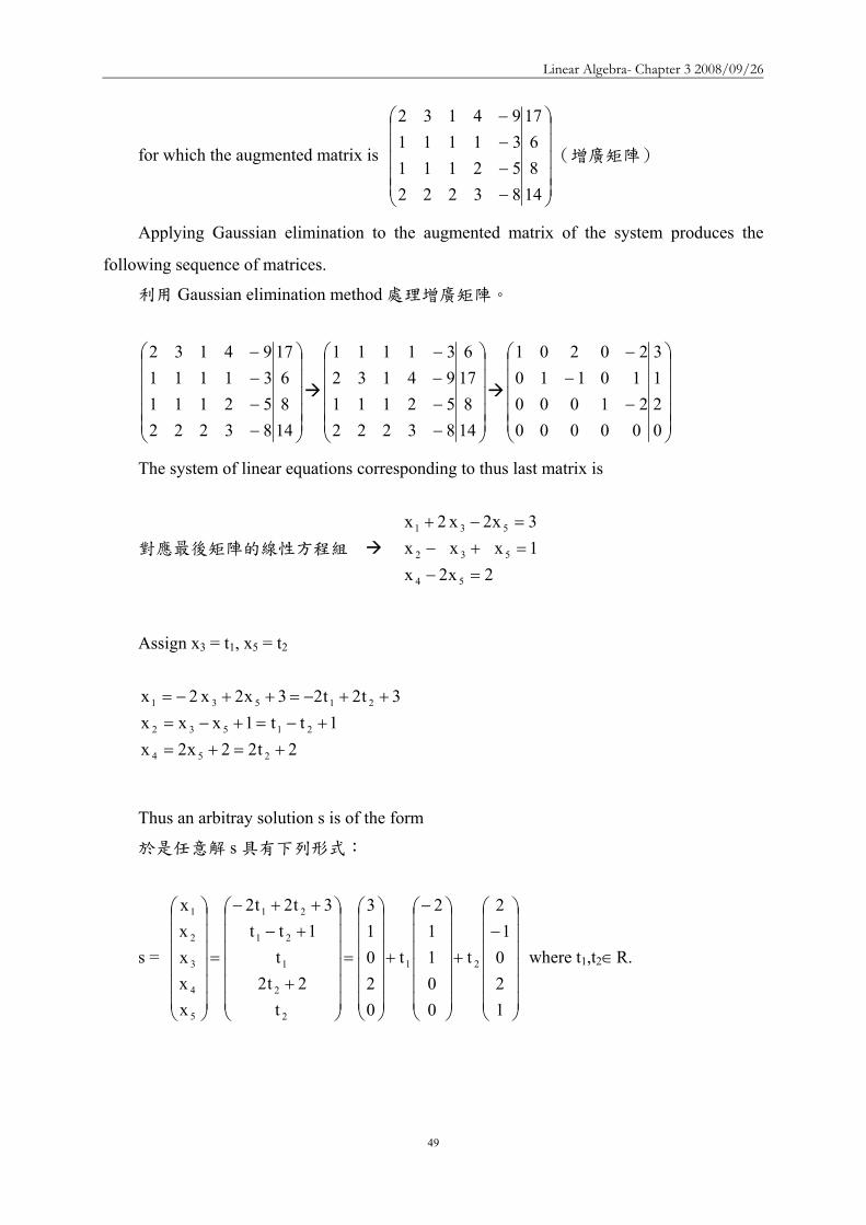
Linear Algebra- Chapter 3 20080926
49
for which the augmented matrix is
⎟⎟⎟⎟⎟
⎠
⎞
⎜⎜⎜⎜⎜
⎝
⎛
minusminusminusminus
1486
17
83222521113111194132
(增廣矩陣)
Applying Gaussian elimination to the augmented matrix of the system produces the
following sequence of matrices
利用 Gaussian elimination method 處理增廣矩陣
⎟⎟⎟⎟⎟
⎠
⎞
⎜⎜⎜⎜⎜
⎝
⎛
minusminusminusminus
1486
17
83222521113111194132
⎟⎟⎟⎟⎟
⎠
⎞
⎜⎜⎜⎜⎜
⎝
⎛
minusminusminusminus
148
176
83222521119413231111
⎟⎟⎟⎟⎟
⎠
⎞
⎜⎜⎜⎜⎜
⎝
⎛
minusminus
minus
0213
0000021000
1011020201
The system of linear equations corresponding to thus last matrix is
對應最後矩陣的線性方程組 2x2x
1xxx3x2x2x
54
532
531
=minus=+minus=minus+
Assign x3 = t1 x5 = t2
2t22x2x1tt1xxx
3t2t23x2x2x
254
21532
21531
+=+=+minus=+minus=
++minus=++minus=
Thus an arbitray solution s is of the form
於是任意解 s 具有下列形式
s =
⎟⎟⎟⎟⎟⎟
⎠
⎞
⎜⎜⎜⎜⎜⎜
⎝
⎛minus
+
⎟⎟⎟⎟⎟⎟
⎠
⎞
⎜⎜⎜⎜⎜⎜
⎝
⎛minus
+
⎟⎟⎟⎟⎟⎟
⎠
⎞
⎜⎜⎜⎜⎜⎜
⎝
⎛
=
⎟⎟⎟⎟⎟⎟
⎠
⎞
⎜⎜⎜⎜⎜⎜
⎝
⎛
+
+minus++minus
=
⎟⎟⎟⎟⎟⎟
⎠
⎞
⎜⎜⎜⎜⎜⎜
⎝
⎛
1201
2
t
00112
t
02013
t2t2
t1tt
3t2t2
xxxxx
21
2
2
1
21
21
5
4
3
2
1
where t1t2isinR
Linear Algebra- Chapter 3 20080926
50
Notice that
⎪⎪⎪
⎭
⎪⎪⎪
⎬
⎫
⎪⎪⎪
⎩
⎪⎪⎪
⎨
⎧
⎟⎟⎟⎟⎟⎟
⎠
⎞
⎜⎜⎜⎜⎜⎜
⎝
⎛minus
⎟⎟⎟⎟⎟⎟
⎠
⎞
⎜⎜⎜⎜⎜⎜
⎝
⎛minus
1201
2
00112
is a basis for the solution set of the corresponding
homogeneous system of equation and
⎟⎟⎟⎟⎟⎟
⎠
⎞
⎜⎜⎜⎜⎜⎜
⎝
⎛
02013
is a particular solution to the original system
⎪⎪⎪
⎭
⎪⎪⎪
⎬
⎫
⎪⎪⎪
⎩
⎪⎪⎪
⎨
⎧
⎟⎟⎟⎟⎟⎟
⎠
⎞
⎜⎜⎜⎜⎜⎜
⎝
⎛minus
⎟⎟⎟⎟⎟⎟
⎠
⎞
⎜⎜⎜⎜⎜⎜
⎝
⎛minus
1201
2
00112
是齊次方程組解集合的一組基底
⎟⎟⎟⎟⎟⎟
⎠
⎞
⎜⎜⎜⎜⎜⎜
⎝
⎛
02013
是原方程組的特別解
EXAMPLE 1
The matrix ⎟⎟⎟
⎠
⎞
⎜⎜⎜
⎝
⎛
101010011
is not in reduced row echelon form
因為第一行含有第一個非零元素在第一列但第一行尚含有其他非零元素
The matrix ⎟⎟⎟
⎠
⎞
⎜⎜⎜
⎝
⎛
110010012010
is not in reduced row echelon form
因為第一列第一個非零元素不在第一列第一個非零元素的右邊
The matrix ⎟⎟⎠
⎞⎜⎜⎝
⎛010002
is not in reduced row echelon form
因為第一列的第一個非零元素不是 1
Linear Algebra- Chapter 3 20080926
51
Reduced Echelon FormReduced Echelon Form
⎥⎥⎥
⎦
⎤
⎢⎢⎢
⎣
⎡
910030107001
⎥⎥⎥
⎦
⎤
⎢⎢⎢
⎣
⎡
100001000041
⎥⎥⎥
⎦
⎤
⎢⎢⎢
⎣
⎡
000210801
Not in Reduced Echelon Form
⎥⎥⎥
⎦
⎤
⎢⎢⎢
⎣
⎡
310000004021
⎥⎥⎥
⎦
⎤
⎢⎢⎢
⎣
⎡
100000430003021
⎥⎥⎥⎥
⎦
⎤
⎢⎢⎢⎢
⎣
⎡
0000210030108071
In Reduced Echelon Form
Use GaussUse Gauss--Jordan elimination to Jordan elimination to find reduced echelon formfind reduced echelon form 1313
Step 1 Interchange rows if necessary to bring a nonzero Step 1 Interchange rows if necessary to bring a nonzero element to the top of the first nonzero column This nonzero element to the top of the first nonzero column This nonzero element is called a pivotelement is called a pivot
⎥⎥⎦
⎤
⎢⎢⎣
⎡
minusminus
minus
1211244129333
22200
⎥⎥⎥
⎦
⎤
⎢⎢⎢
⎣
⎡
minusminus
minus
harrasymp
121124422200
129333
R2R1
Use GaussUse Gauss--Jordan elimination to Jordan elimination to find reduced echelon formfind reduced echelon form 2323
Step 2 Create a 1 in the pivot location by multiplying the Step 2 Create a 1 in the pivot location by multiplying the pivot row by 1pivotpivot row by 1pivot
Step 3 Create zero elsewhere in the pivot column by adding Step 3 Create zero elsewhere in the pivot column by adding suitable multiples of the pivot row to all other rows of the suitable multiples of the pivot row to all other rows of the matrixmatrix
⎥⎥⎥
⎦
⎤
⎢⎢⎢
⎣
⎡
minusminusminus
minus
minus+asymp
412002220043111
4)R1(R3
⎥⎥⎦
⎤
⎢⎢⎣
⎡
minusminus
minus
⎟⎠⎞
⎜⎝⎛asymp
12112442220043111
R13
1
The matrix is the reduced echelon form of the given matrixThe matrix is the reduced echelon form of the given matrix
Use GaussUse Gauss--Jordan elimination to Jordan elimination to find reduced echelon formfind reduced echelon form 3333
Step 4 Cover the pivot row and all rows above it Repeat Steps Step 4 Cover the pivot row and all rows above it Repeat Steps 1 1 and 2 for the remaining and 2 for the remaining submatrixsubmatrix Repeat Step 3 for the whole Repeat Step 3 for the whole matrix Continue until the reduced echelon form is reachedmatrix Continue until the reduced echelon form is reached
⎥⎥⎥
⎦
⎤
⎢⎢⎢
⎣
⎡
minusminus
+minus+asymp
⎥⎥⎥
⎦
⎤
⎢⎢⎢
⎣
⎡
minusminus
minus++asymp
⎥⎥⎥
⎦
⎤
⎢⎢⎢
⎣
⎡
minusminusminus
minus
⎟⎠⎞
⎜⎝⎛
asymp
⎥⎥⎥
⎦
⎤
⎢⎢⎢
⎣
⎡
minusminusminus
minus
6100050100
170011
R3R22)R3(R1
610001110052011
R2)2(R3R2R1
412001110043111
R221
412002220043111
Theorem 315 Let Ax = b be a system of r nonzero equations is in n unknown Suppose that rank(A)
= rank (A b)∣ and that (A b)∣ is in reduced row echelon form Then
設 Ax = b 為含有 n 個未知數r 個非零方程式的方程組假設 rank(A) = rank
(A b)∣ 且 (A b)∣ 為簡約列梯形式於是
(a) rank(A) = r
(b) If the general solution obtained by the procedure above is of the form s = s0 + t1u1
+ t2u2 +hellip+ tn-run-r then u1 u2hellip un-r is a basis for the solution set of the
corresponding homogeneous system and s0 is a solution to the original system 由
前述方法所得的 General solution 具有下列形式
s = s0 + t1u1 + t2u2 +hellip+ tn-run-r
其中u1 u2hellip un-r為齊次方程組 Ax = 0 的解集合的一組基底且 s0 為原方
程組的一個解)
【Proof】
Since (A b)∣ is in reduced row echelon form (A b)∣ must have r nonzero rows
Clearly these rows are linearly independent by the definition of the reduced row echelon
Linear Algebra- Chapter 3 20080926
52
form and so rank (A b)∣ = r Thus rank(A) = r
Let K be the solution set for Ax = b and let KH be the solution set for Ax = 0 Setting
t1 = t2 =hellip= tn-r = 0 we see that s = s0isinK But by Theorem 39 K = s +KH Hence
KH = - s0+K = span(u1 u2hellip un-r )
Because rank(A) = r we have dim(KH) = n-r Thus since dim(KH) = n-r and KH is
generated by a set u1 u2hellip un-r containing at most n-r vectors that is a basis for KH
由於(A b)∣ 具有簡約列梯形式因此(A b)∣ 必定具有 r 個非零列由簡約列梯形
式的定義得知 r 個非零列為線性獨立故 rank (A b)∣ = rrank(A) = r
令 K 為 Ax = b 的解集合 KH 為 Ax = 0 的解集合
假設 t1 = t2 =hellip= tn-r = 0(u1 u2hellip un-r非 KH的基底)則 s = s0isinK
依據 Theorem 39K = s +KH KH = - s0+K = span(u1 u2hellip un-r )
因 rank(A) = r所以 dim(KH) = n - r 且 KH 是由u1 u2hellip un-r 所生成
故原假設「t1 = t2 =hellip= tn-r = 0」不成立
因此 KH含有最多 n - r 個向量且這些向量為 KH的基底
Theorem 39 Let K be the solution set of a system of linear equations Ax = b and let KH be
the solution set of the corresponding homogeneous system Ax = 0 Then for any solution s
to Ax = b K =s + KH = s+k kisinKH 設 K 為線性方程組 Ax = b 的解集合且 KH
為對應的齊次方程組的解集合則對 Ax = b 的任一個解 s 而言K =s + KH = s+k
kisinKH
ExampleExampleSolve the system of equationsSolve the system of equations
7537429333
321
321
321
=minusminus=+minus=+minus
xxxxxxxxx
⎥⎥⎦
⎤
⎢⎢⎣
⎡
++asymp
000012104301
R2R3R2R1 12
431243
32
31
32
31+minus=+minus=rArr=+
=+rArr xxxx
xxxx
The general solution to the system isThe general solution to the system is
parameter) a (callednumber real is where 1243
3
2
1
rrxrxrx
=+minus=+minus=
⎥⎥⎥
⎦
⎤
⎢⎢⎢
⎣
⎡
minusminusminus
minus
minus+minus+asymp
⎥⎥⎥
⎦
⎤
⎢⎢⎢
⎣
⎡
minusminusminusminus
asymp
⎥⎥⎥
⎦
⎤
⎢⎢⎢
⎣
⎡
minusminusminusminus
242012103111
1R)3(3R1R)2(2R
715374123111
715374129333
R131
ExampleExample
Solve the system of equationsSolve the system of equations446942
1423258101242
4321
4321
4321
=minus+minusminus=+minus+minus
=minus+minus
xxxxxxxxxxxx
⎪⎪
⎩
⎪⎪
⎨
⎧
===
minus=
rArr==minus=minus
rArr
1x6xrx
2r2x
1x6x
2x2x
4
3
2
1
4
3
21
⎥⎥⎥
⎦
⎤
⎢⎢⎢
⎣
⎡ minusminusasymp
⎥⎥⎥
⎦
⎤
⎢⎢⎢
⎣
⎡minus
minusminusasymp
⎥⎥⎥
⎦
⎤
⎢⎢⎢
⎣
⎡
minusminusminusminusminusasymp
⎥⎥⎥
⎦
⎤
⎢⎢⎢
⎣
⎡
minusminusminusminusminusasymp
⎥⎥⎥
⎦
⎤
⎢⎢⎢
⎣
⎡
minusminusminusminusminus
minusminusasymp
⎥⎥⎥
⎦
⎤
⎢⎢⎢
⎣
⎡
minusminusminusminusminus
minusminus
+
minus+
+
minus+
minus+
+
110006010020021
110005110011021
14430051100
295621
2R31
144300153300295621
446942142321295621
44694214232158101242
R3R2
1)R3(R1
3R2R3
6)R2(R1
2)R1(R3
R1R2R1
21
Linear Algebra- Chapter 3 20080926
53
ExampleExampleSolve the system of equationsSolve the system of equations
432636242232
54321
54321
54321
=+minus+minusminus=++minus+=++minus+
xxxxxxxxxxxxxxx
⎥⎥⎦
⎤
⎢⎢⎣
⎡ minusasymp
⎥⎥⎦
⎤
⎢⎢⎣
⎡
minusminusminusminusminus
+
minus+
642000210000213121
431121636242213121
R1R3
2)R1(R2
⎥⎥⎦
⎤
⎢⎢⎣
⎡ minusasympharr 210000
642000213121
R3R2 ( ) ⎥⎥⎦
⎤
⎢⎢⎣
⎡ minusasymp
210000321000213121
2R21
⎥⎥⎦
⎤
⎢⎢⎣
⎡ minusminusminusasympminus+ 210000
321000750121
3)R2(R1 ⎥⎥⎦
⎤
⎢⎢⎣
⎡minus
minusasymp
minus+
+
210000101000300121
2)R3(R2
5R3R1
2x1x
3xx2x
5
4
321
=minus=
++minus=rArr
2xs and r somefor 1x sx rx
3sr2x
5
432
1
=minus===
++minus=
ExampleExample
Solve the system of Solve the system of equationsequations 122
32452232
32
321
321
321
=+minus=minus+
=+minus=+minus
xxxxxxxxxxx
⎥⎥
⎦
⎤
⎢⎢
⎣
⎡asymp
minusminusminus
minus
harr1220210063303211
R3R2
( ) ⎥⎥
⎦
⎤
⎢⎢
⎣
⎡asymp
minusminusminus
minus
1220210021103211
R231
⎥⎥
⎦
⎤
⎢⎢
⎣
⎡asympminusminusminus
minus+
+
5400210021101101
2)R2(R4
R2R1 ⎥⎥
⎦
⎤
⎢⎢
⎣
⎡asymp
minusminus
minus+
+
minus+
13000210040103001
4)R3R(R4
R3R2
1)R3(R1
( ) ⎥⎥
⎦
⎤
⎢⎢
⎣
⎡asymp
minusminus
1000210040103001
R4131
The system has no solutionThe system has no solution
⎥⎥
⎦
⎤
⎢⎢
⎣
⎡asymp
⎥⎥
⎦
⎤
⎢⎢
⎣
⎡
minusminusminus
minus
minusminusminusminus
minus+
minus+
1220633021003211
1220312145223211
1)R1(R3
2)R1(R2
0x1+0x2+0x3=1
Curve FittingCurve Fitting
A set of data points A set of data points is given and it is is given and it is necessary to find a polynomial whose graph passes through the necessary to find a polynomial whose graph passes through the points points The points are often measurements in an experiment The points are often measurements in an experiment The xThe x--coordinates are called coordinates are called base pointsbase pointsIt can be shown that if the base points are all distinct then aIt can be shown that if the base points are all distinct then a unique unique polynomial of degree n polynomial of degree n ndashndash 1 (or less)1 (or less)
can be fitted to thecan be fitted to the pointspoints
) ( ) ( ) ( 2211 nn yxyxyx K
11
2210
minusminus
minusminus ++++= n
nn
n xaxaxaay K
The coefficients can be found by substituting the points The coefficients can be found by substituting the points into the polynomial equation and then solving a system into the polynomial equation and then solving a system of linear equationsof linear equations
ExampleExample
Determine the equation of the polynomial of degree 2 whose graphpasses through the points (1 6) (2 3) (3 2)
Let the polynomial be and substituting x = 1 y = 6 x = 2 y = 3 x = 3 y = 2 we have
Solving this system for a0 a1 and a2 using Gauss-Jordan elimination
⎥⎥⎥
⎦
⎤
⎢⎢⎢
⎣
⎡minus
minus
minus+minus+asymp
220033109201
1)R2(R31)R2(R1
2210 xaxaay ++=
2a9a3a3a4a2a6aaa
210
210
210
=++=++=++
⎥⎥⎥
⎦
⎤
⎢⎢⎢
⎣
⎡
minusminus
⎥⎥⎥
⎦
⎤
⎢⎢⎢
⎣
⎡
minus+minus+asymp
482033106111
293134216111
1)R1(R31)R1(R2
( )⎥⎥⎥
⎦
⎤
⎢⎢⎢
⎣
⎡minus
⎥⎥⎥
⎦
⎤
⎢⎢⎢
⎣
⎡minus
minusasymp
minus++asymp
11006010
11001
110033109201
3)R3(R22R3R1
R321
We get a0 = 11 a1 = ndash 6 a2 = 1The parabola that passes through these points is y = 11 ndash 6x + x2
ExampleExample Traffic FlowTraffic Flow
Network analysis plays an important role in electrical Network analysis plays an important role in electrical engineeringengineeringThe concepts and tools of network analysis have been The concepts and tools of network analysis have been found to be useful in many other fields such as found to be useful in many other fields such as information theory and the study of transportation systemsinformation theory and the study of transportation systemsThe analysis of traffic flow through a road network during The analysis of traffic flow through a road network during peak period illustrates how systems of linear equations peak period illustrates how systems of linear equations with with manymany solutions can arise in practicesolutions can arise in practice
Traffic FlowTraffic Flow
Consider the typical road network The streets are all oneConsider the typical road network The streets are all one--way with the arrows indicating the direction of traffic flowway with the arrows indicating the direction of traffic flowThe flow of traffic in and out of the network is measured The flow of traffic in and out of the network is measured in vehicles per hour (in vehicles per hour (vphvph))How to construct a mathematical model to analyze this How to construct a mathematical model to analyze this network network
Traffic Traffic FlowFlowTRAFFIC LAWTRAFFIC LAWhelliphellipAll traffic entering an intersection must leave that All traffic entering an intersection must leave that intersectionintersection
Linear Algebra- Chapter 3 20080926
54
Junction AJunction BJunction CJunction DJunction EJunction F 600
800 200 500 100 600
54
643
73
72
621
51
=+=++minus=+minus=minus=+minus=+
xxxxx
xxxx
xxxxx
⎥⎥⎥⎥⎥⎥⎥⎥⎥⎥⎥⎥⎥
⎦
⎤
⎢⎢⎢⎢⎢⎢⎢⎢⎢⎢⎢⎢⎢
⎣
⎡
asympasymp
⎥⎥⎥⎥⎥⎥⎥⎥⎥⎥⎥⎥⎥
⎦
⎤
⎢⎢⎢⎢⎢⎢⎢⎢⎢⎢⎢⎢⎢
⎣
⎡
minusminus
minusminusminusminus
minusminus
minusminus
0000000001110000
6001101000200100010050010000106001100001
600001100080001011002001000100500100001010001000116000010001
L
Traffic FlowTraffic FlowJunction AJunction BJunction CJunction DJunction EJunction F 600
800 200 500 100 600
54
643
73
72
621
51
=+=++minus=+minus=minus=+minus=+
xxxxx
xxxx
xxxxx
Perform road work on x7 Because x3 ge 0 the minimum flow 200 in the branch x7 can be obtained by making x3 = 0 (closing DE to traffic)
Traffic FlowTraffic Flow
We get
765
76473
72761
xx x600xxx200x x500x x600xxx
minus=++minus=minus=+=+minusminus=
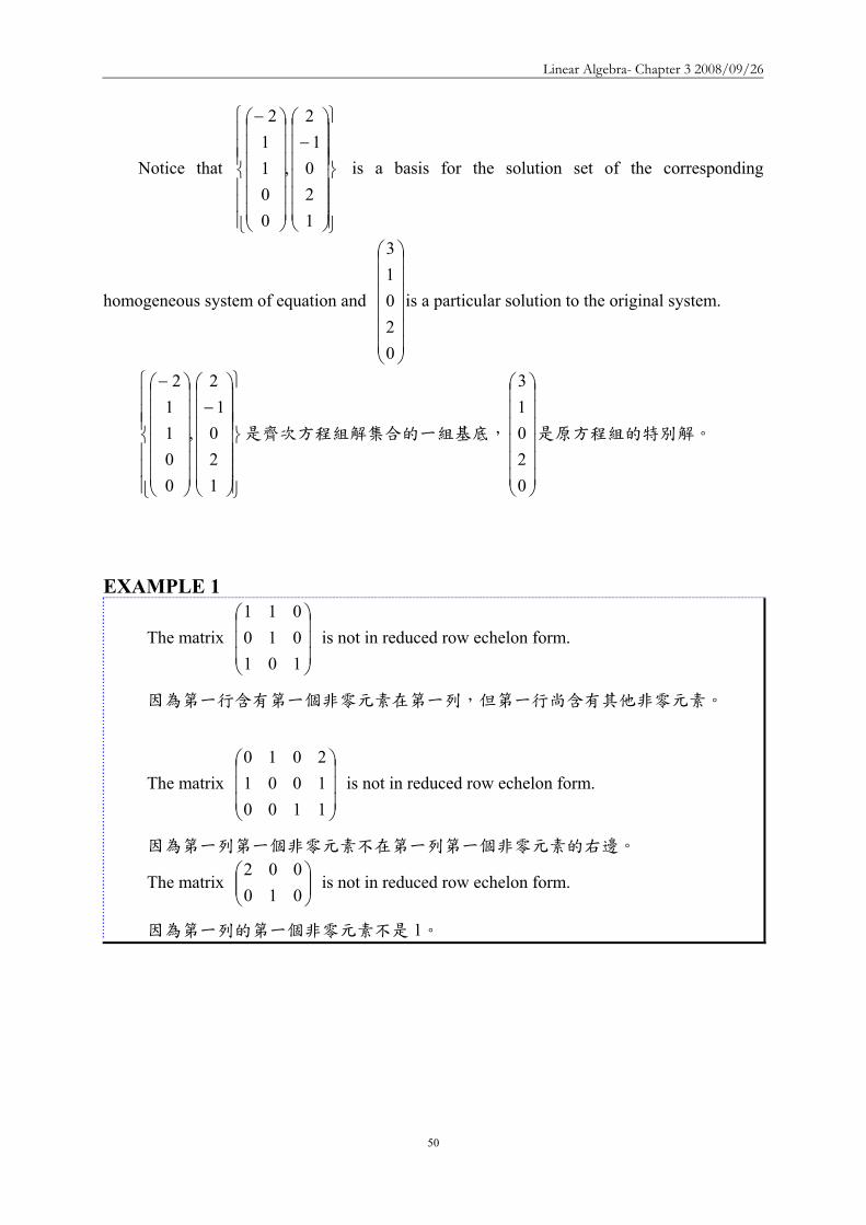
Linear Algebra- Chapter 3 20080926
51
Reduced Echelon FormReduced Echelon Form
⎥⎥⎥
⎦
⎤
⎢⎢⎢
⎣
⎡
910030107001
⎥⎥⎥
⎦
⎤
⎢⎢⎢
⎣
⎡
100001000041
⎥⎥⎥
⎦
⎤
⎢⎢⎢
⎣
⎡
000210801
Not in Reduced Echelon Form
⎥⎥⎥
⎦
⎤
⎢⎢⎢
⎣
⎡
310000004021
⎥⎥⎥
⎦
⎤
⎢⎢⎢
⎣
⎡
100000430003021
⎥⎥⎥⎥
⎦
⎤
⎢⎢⎢⎢
⎣
⎡
0000210030108071
In Reduced Echelon Form
Use GaussUse Gauss--Jordan elimination to Jordan elimination to find reduced echelon formfind reduced echelon form 1313
Step 1 Interchange rows if necessary to bring a nonzero Step 1 Interchange rows if necessary to bring a nonzero element to the top of the first nonzero column This nonzero element to the top of the first nonzero column This nonzero element is called a pivotelement is called a pivot
⎥⎥⎦
⎤
⎢⎢⎣
⎡
minusminus
minus
1211244129333
22200
⎥⎥⎥
⎦
⎤
⎢⎢⎢
⎣
⎡
minusminus
minus
harrasymp
121124422200
129333
R2R1
Use GaussUse Gauss--Jordan elimination to Jordan elimination to find reduced echelon formfind reduced echelon form 2323
Step 2 Create a 1 in the pivot location by multiplying the Step 2 Create a 1 in the pivot location by multiplying the pivot row by 1pivotpivot row by 1pivot
Step 3 Create zero elsewhere in the pivot column by adding Step 3 Create zero elsewhere in the pivot column by adding suitable multiples of the pivot row to all other rows of the suitable multiples of the pivot row to all other rows of the matrixmatrix
⎥⎥⎥
⎦
⎤
⎢⎢⎢
⎣
⎡
minusminusminus
minus
minus+asymp
412002220043111
4)R1(R3
⎥⎥⎦
⎤
⎢⎢⎣
⎡
minusminus
minus
⎟⎠⎞
⎜⎝⎛asymp
12112442220043111
R13
1
The matrix is the reduced echelon form of the given matrixThe matrix is the reduced echelon form of the given matrix
Use GaussUse Gauss--Jordan elimination to Jordan elimination to find reduced echelon formfind reduced echelon form 3333
Step 4 Cover the pivot row and all rows above it Repeat Steps Step 4 Cover the pivot row and all rows above it Repeat Steps 1 1 and 2 for the remaining and 2 for the remaining submatrixsubmatrix Repeat Step 3 for the whole Repeat Step 3 for the whole matrix Continue until the reduced echelon form is reachedmatrix Continue until the reduced echelon form is reached
⎥⎥⎥
⎦
⎤
⎢⎢⎢
⎣
⎡
minusminus
+minus+asymp
⎥⎥⎥
⎦
⎤
⎢⎢⎢
⎣
⎡
minusminus
minus++asymp
⎥⎥⎥
⎦
⎤
⎢⎢⎢
⎣
⎡
minusminusminus
minus
⎟⎠⎞
⎜⎝⎛
asymp
⎥⎥⎥
⎦
⎤
⎢⎢⎢
⎣
⎡
minusminusminus
minus
6100050100
170011
R3R22)R3(R1
610001110052011
R2)2(R3R2R1
412001110043111
R221
412002220043111
Theorem 315 Let Ax = b be a system of r nonzero equations is in n unknown Suppose that rank(A)
= rank (A b)∣ and that (A b)∣ is in reduced row echelon form Then
設 Ax = b 為含有 n 個未知數r 個非零方程式的方程組假設 rank(A) = rank
(A b)∣ 且 (A b)∣ 為簡約列梯形式於是
(a) rank(A) = r
(b) If the general solution obtained by the procedure above is of the form s = s0 + t1u1
+ t2u2 +hellip+ tn-run-r then u1 u2hellip un-r is a basis for the solution set of the
corresponding homogeneous system and s0 is a solution to the original system 由
前述方法所得的 General solution 具有下列形式
s = s0 + t1u1 + t2u2 +hellip+ tn-run-r
其中u1 u2hellip un-r為齊次方程組 Ax = 0 的解集合的一組基底且 s0 為原方
程組的一個解)
【Proof】
Since (A b)∣ is in reduced row echelon form (A b)∣ must have r nonzero rows
Clearly these rows are linearly independent by the definition of the reduced row echelon
Linear Algebra- Chapter 3 20080926
52
form and so rank (A b)∣ = r Thus rank(A) = r
Let K be the solution set for Ax = b and let KH be the solution set for Ax = 0 Setting
t1 = t2 =hellip= tn-r = 0 we see that s = s0isinK But by Theorem 39 K = s +KH Hence
KH = - s0+K = span(u1 u2hellip un-r )
Because rank(A) = r we have dim(KH) = n-r Thus since dim(KH) = n-r and KH is
generated by a set u1 u2hellip un-r containing at most n-r vectors that is a basis for KH
由於(A b)∣ 具有簡約列梯形式因此(A b)∣ 必定具有 r 個非零列由簡約列梯形
式的定義得知 r 個非零列為線性獨立故 rank (A b)∣ = rrank(A) = r
令 K 為 Ax = b 的解集合 KH 為 Ax = 0 的解集合
假設 t1 = t2 =hellip= tn-r = 0(u1 u2hellip un-r非 KH的基底)則 s = s0isinK
依據 Theorem 39K = s +KH KH = - s0+K = span(u1 u2hellip un-r )
因 rank(A) = r所以 dim(KH) = n - r 且 KH 是由u1 u2hellip un-r 所生成
故原假設「t1 = t2 =hellip= tn-r = 0」不成立
因此 KH含有最多 n - r 個向量且這些向量為 KH的基底
Theorem 39 Let K be the solution set of a system of linear equations Ax = b and let KH be
the solution set of the corresponding homogeneous system Ax = 0 Then for any solution s
to Ax = b K =s + KH = s+k kisinKH 設 K 為線性方程組 Ax = b 的解集合且 KH
為對應的齊次方程組的解集合則對 Ax = b 的任一個解 s 而言K =s + KH = s+k
kisinKH
ExampleExampleSolve the system of equationsSolve the system of equations
7537429333
321
321
321
=minusminus=+minus=+minus
xxxxxxxxx
⎥⎥⎦
⎤
⎢⎢⎣
⎡
++asymp
000012104301
R2R3R2R1 12
431243
32
31
32
31+minus=+minus=rArr=+
=+rArr xxxx
xxxx
The general solution to the system isThe general solution to the system is
parameter) a (callednumber real is where 1243
3
2
1
rrxrxrx
=+minus=+minus=
⎥⎥⎥
⎦
⎤
⎢⎢⎢
⎣
⎡
minusminusminus
minus
minus+minus+asymp
⎥⎥⎥
⎦
⎤
⎢⎢⎢
⎣
⎡
minusminusminusminus
asymp
⎥⎥⎥
⎦
⎤
⎢⎢⎢
⎣
⎡
minusminusminusminus
242012103111
1R)3(3R1R)2(2R
715374123111
715374129333
R131
ExampleExample
Solve the system of equationsSolve the system of equations446942
1423258101242
4321
4321
4321
=minus+minusminus=+minus+minus
=minus+minus
xxxxxxxxxxxx
⎪⎪
⎩
⎪⎪
⎨
⎧
===
minus=
rArr==minus=minus
rArr
1x6xrx
2r2x
1x6x
2x2x
4
3
2
1
4
3
21
⎥⎥⎥
⎦
⎤
⎢⎢⎢
⎣
⎡ minusminusasymp
⎥⎥⎥
⎦
⎤
⎢⎢⎢
⎣
⎡minus
minusminusasymp
⎥⎥⎥
⎦
⎤
⎢⎢⎢
⎣
⎡
minusminusminusminusminusasymp
⎥⎥⎥
⎦
⎤
⎢⎢⎢
⎣
⎡
minusminusminusminusminusasymp
⎥⎥⎥
⎦
⎤
⎢⎢⎢
⎣
⎡
minusminusminusminusminus
minusminusasymp
⎥⎥⎥
⎦
⎤
⎢⎢⎢
⎣
⎡
minusminusminusminusminus
minusminus
+
minus+
+
minus+
minus+
+
110006010020021
110005110011021
14430051100
295621
2R31
144300153300295621
446942142321295621
44694214232158101242
R3R2
1)R3(R1
3R2R3
6)R2(R1
2)R1(R3
R1R2R1
21
Linear Algebra- Chapter 3 20080926
53
ExampleExampleSolve the system of equationsSolve the system of equations
432636242232
54321
54321
54321
=+minus+minusminus=++minus+=++minus+
xxxxxxxxxxxxxxx
⎥⎥⎦
⎤
⎢⎢⎣
⎡ minusasymp
⎥⎥⎦
⎤
⎢⎢⎣
⎡
minusminusminusminusminus
+
minus+
642000210000213121
431121636242213121
R1R3
2)R1(R2
⎥⎥⎦
⎤
⎢⎢⎣
⎡ minusasympharr 210000
642000213121
R3R2 ( ) ⎥⎥⎦
⎤
⎢⎢⎣
⎡ minusasymp
210000321000213121
2R21
⎥⎥⎦
⎤
⎢⎢⎣
⎡ minusminusminusasympminus+ 210000
321000750121
3)R2(R1 ⎥⎥⎦
⎤
⎢⎢⎣
⎡minus
minusasymp
minus+
+
210000101000300121
2)R3(R2
5R3R1
2x1x
3xx2x
5
4
321
=minus=
++minus=rArr
2xs and r somefor 1x sx rx
3sr2x
5
432
1
=minus===
++minus=
ExampleExample
Solve the system of Solve the system of equationsequations 122
32452232
32
321
321
321
=+minus=minus+
=+minus=+minus
xxxxxxxxxxx
⎥⎥
⎦
⎤
⎢⎢
⎣
⎡asymp
minusminusminus
minus
harr1220210063303211
R3R2
( ) ⎥⎥
⎦
⎤
⎢⎢
⎣
⎡asymp
minusminusminus
minus
1220210021103211
R231
⎥⎥
⎦
⎤
⎢⎢
⎣
⎡asympminusminusminus
minus+
+
5400210021101101
2)R2(R4
R2R1 ⎥⎥
⎦
⎤
⎢⎢
⎣
⎡asymp
minusminus
minus+
+
minus+
13000210040103001
4)R3R(R4
R3R2
1)R3(R1
( ) ⎥⎥
⎦
⎤
⎢⎢
⎣
⎡asymp
minusminus
1000210040103001
R4131
The system has no solutionThe system has no solution
⎥⎥
⎦
⎤
⎢⎢
⎣
⎡asymp
⎥⎥
⎦
⎤
⎢⎢
⎣
⎡
minusminusminus
minus
minusminusminusminus
minus+
minus+
1220633021003211
1220312145223211
1)R1(R3
2)R1(R2
0x1+0x2+0x3=1
Curve FittingCurve Fitting
A set of data points A set of data points is given and it is is given and it is necessary to find a polynomial whose graph passes through the necessary to find a polynomial whose graph passes through the points points The points are often measurements in an experiment The points are often measurements in an experiment The xThe x--coordinates are called coordinates are called base pointsbase pointsIt can be shown that if the base points are all distinct then aIt can be shown that if the base points are all distinct then a unique unique polynomial of degree n polynomial of degree n ndashndash 1 (or less)1 (or less)
can be fitted to thecan be fitted to the pointspoints
) ( ) ( ) ( 2211 nn yxyxyx K
11
2210
minusminus
minusminus ++++= n
nn
n xaxaxaay K
The coefficients can be found by substituting the points The coefficients can be found by substituting the points into the polynomial equation and then solving a system into the polynomial equation and then solving a system of linear equationsof linear equations
ExampleExample
Determine the equation of the polynomial of degree 2 whose graphpasses through the points (1 6) (2 3) (3 2)
Let the polynomial be and substituting x = 1 y = 6 x = 2 y = 3 x = 3 y = 2 we have
Solving this system for a0 a1 and a2 using Gauss-Jordan elimination
⎥⎥⎥
⎦
⎤
⎢⎢⎢
⎣
⎡minus
minus
minus+minus+asymp
220033109201
1)R2(R31)R2(R1
2210 xaxaay ++=
2a9a3a3a4a2a6aaa
210
210
210
=++=++=++
⎥⎥⎥
⎦
⎤
⎢⎢⎢
⎣
⎡
minusminus
⎥⎥⎥
⎦
⎤
⎢⎢⎢
⎣
⎡
minus+minus+asymp
482033106111
293134216111
1)R1(R31)R1(R2
( )⎥⎥⎥
⎦
⎤
⎢⎢⎢
⎣
⎡minus
⎥⎥⎥
⎦
⎤
⎢⎢⎢
⎣
⎡minus
minusasymp
minus++asymp
11006010
11001
110033109201
3)R3(R22R3R1
R321
We get a0 = 11 a1 = ndash 6 a2 = 1The parabola that passes through these points is y = 11 ndash 6x + x2
ExampleExample Traffic FlowTraffic Flow
Network analysis plays an important role in electrical Network analysis plays an important role in electrical engineeringengineeringThe concepts and tools of network analysis have been The concepts and tools of network analysis have been found to be useful in many other fields such as found to be useful in many other fields such as information theory and the study of transportation systemsinformation theory and the study of transportation systemsThe analysis of traffic flow through a road network during The analysis of traffic flow through a road network during peak period illustrates how systems of linear equations peak period illustrates how systems of linear equations with with manymany solutions can arise in practicesolutions can arise in practice
Traffic FlowTraffic Flow
Consider the typical road network The streets are all oneConsider the typical road network The streets are all one--way with the arrows indicating the direction of traffic flowway with the arrows indicating the direction of traffic flowThe flow of traffic in and out of the network is measured The flow of traffic in and out of the network is measured in vehicles per hour (in vehicles per hour (vphvph))How to construct a mathematical model to analyze this How to construct a mathematical model to analyze this network network
Traffic Traffic FlowFlowTRAFFIC LAWTRAFFIC LAWhelliphellipAll traffic entering an intersection must leave that All traffic entering an intersection must leave that intersectionintersection
Linear Algebra- Chapter 3 20080926
54
Junction AJunction BJunction CJunction DJunction EJunction F 600
800 200 500 100 600
54
643
73
72
621
51
=+=++minus=+minus=minus=+minus=+
xxxxx
xxxx
xxxxx
⎥⎥⎥⎥⎥⎥⎥⎥⎥⎥⎥⎥⎥
⎦
⎤
⎢⎢⎢⎢⎢⎢⎢⎢⎢⎢⎢⎢⎢
⎣
⎡
asympasymp
⎥⎥⎥⎥⎥⎥⎥⎥⎥⎥⎥⎥⎥
⎦
⎤
⎢⎢⎢⎢⎢⎢⎢⎢⎢⎢⎢⎢⎢
⎣
⎡
minusminus
minusminusminusminus
minusminus
minusminus
0000000001110000
6001101000200100010050010000106001100001
600001100080001011002001000100500100001010001000116000010001
L
Traffic FlowTraffic FlowJunction AJunction BJunction CJunction DJunction EJunction F 600
800 200 500 100 600
54
643
73
72
621
51
=+=++minus=+minus=minus=+minus=+
xxxxx
xxxx
xxxxx
Perform road work on x7 Because x3 ge 0 the minimum flow 200 in the branch x7 can be obtained by making x3 = 0 (closing DE to traffic)
Traffic FlowTraffic Flow
We get
765
76473
72761
xx x600xxx200x x500x x600xxx
minus=++minus=minus=+=+minusminus=

Linear Algebra- Chapter 3 20080926
52
form and so rank (A b)∣ = r Thus rank(A) = r
Let K be the solution set for Ax = b and let KH be the solution set for Ax = 0 Setting
t1 = t2 =hellip= tn-r = 0 we see that s = s0isinK But by Theorem 39 K = s +KH Hence
KH = - s0+K = span(u1 u2hellip un-r )
Because rank(A) = r we have dim(KH) = n-r Thus since dim(KH) = n-r and KH is
generated by a set u1 u2hellip un-r containing at most n-r vectors that is a basis for KH
由於(A b)∣ 具有簡約列梯形式因此(A b)∣ 必定具有 r 個非零列由簡約列梯形
式的定義得知 r 個非零列為線性獨立故 rank (A b)∣ = rrank(A) = r
令 K 為 Ax = b 的解集合 KH 為 Ax = 0 的解集合
假設 t1 = t2 =hellip= tn-r = 0(u1 u2hellip un-r非 KH的基底)則 s = s0isinK
依據 Theorem 39K = s +KH KH = - s0+K = span(u1 u2hellip un-r )
因 rank(A) = r所以 dim(KH) = n - r 且 KH 是由u1 u2hellip un-r 所生成
故原假設「t1 = t2 =hellip= tn-r = 0」不成立
因此 KH含有最多 n - r 個向量且這些向量為 KH的基底
Theorem 39 Let K be the solution set of a system of linear equations Ax = b and let KH be
the solution set of the corresponding homogeneous system Ax = 0 Then for any solution s
to Ax = b K =s + KH = s+k kisinKH 設 K 為線性方程組 Ax = b 的解集合且 KH
為對應的齊次方程組的解集合則對 Ax = b 的任一個解 s 而言K =s + KH = s+k
kisinKH
ExampleExampleSolve the system of equationsSolve the system of equations
7537429333
321
321
321
=minusminus=+minus=+minus
xxxxxxxxx
⎥⎥⎦
⎤
⎢⎢⎣
⎡
++asymp
000012104301
R2R3R2R1 12
431243
32
31
32
31+minus=+minus=rArr=+
=+rArr xxxx
xxxx
The general solution to the system isThe general solution to the system is
parameter) a (callednumber real is where 1243
3
2
1
rrxrxrx
=+minus=+minus=
⎥⎥⎥
⎦
⎤
⎢⎢⎢
⎣
⎡
minusminusminus
minus
minus+minus+asymp
⎥⎥⎥
⎦
⎤
⎢⎢⎢
⎣
⎡
minusminusminusminus
asymp
⎥⎥⎥
⎦
⎤
⎢⎢⎢
⎣
⎡
minusminusminusminus
242012103111
1R)3(3R1R)2(2R
715374123111
715374129333
R131
ExampleExample
Solve the system of equationsSolve the system of equations446942
1423258101242
4321
4321
4321
=minus+minusminus=+minus+minus
=minus+minus
xxxxxxxxxxxx
⎪⎪
⎩
⎪⎪
⎨
⎧
===
minus=
rArr==minus=minus
rArr
1x6xrx
2r2x
1x6x
2x2x
4
3
2
1
4
3
21
⎥⎥⎥
⎦
⎤
⎢⎢⎢
⎣
⎡ minusminusasymp
⎥⎥⎥
⎦
⎤
⎢⎢⎢
⎣
⎡minus
minusminusasymp
⎥⎥⎥
⎦
⎤
⎢⎢⎢
⎣
⎡
minusminusminusminusminusasymp
⎥⎥⎥
⎦
⎤
⎢⎢⎢
⎣
⎡
minusminusminusminusminusasymp
⎥⎥⎥
⎦
⎤
⎢⎢⎢
⎣
⎡
minusminusminusminusminus
minusminusasymp
⎥⎥⎥
⎦
⎤
⎢⎢⎢
⎣
⎡
minusminusminusminusminus
minusminus
+
minus+
+
minus+
minus+
+
110006010020021
110005110011021
14430051100
295621
2R31
144300153300295621
446942142321295621
44694214232158101242
R3R2
1)R3(R1
3R2R3
6)R2(R1
2)R1(R3
R1R2R1
21
Linear Algebra- Chapter 3 20080926
53
ExampleExampleSolve the system of equationsSolve the system of equations
432636242232
54321
54321
54321
=+minus+minusminus=++minus+=++minus+
xxxxxxxxxxxxxxx
⎥⎥⎦
⎤
⎢⎢⎣
⎡ minusasymp
⎥⎥⎦
⎤
⎢⎢⎣
⎡
minusminusminusminusminus
+
minus+
642000210000213121
431121636242213121
R1R3
2)R1(R2
⎥⎥⎦
⎤
⎢⎢⎣
⎡ minusasympharr 210000
642000213121
R3R2 ( ) ⎥⎥⎦
⎤
⎢⎢⎣
⎡ minusasymp
210000321000213121
2R21
⎥⎥⎦
⎤
⎢⎢⎣
⎡ minusminusminusasympminus+ 210000
321000750121
3)R2(R1 ⎥⎥⎦
⎤
⎢⎢⎣
⎡minus
minusasymp
minus+
+
210000101000300121
2)R3(R2
5R3R1
2x1x
3xx2x
5
4
321
=minus=
++minus=rArr
2xs and r somefor 1x sx rx
3sr2x
5
432
1
=minus===
++minus=
ExampleExample
Solve the system of Solve the system of equationsequations 122
32452232
32
321
321
321
=+minus=minus+
=+minus=+minus
xxxxxxxxxxx
⎥⎥
⎦
⎤
⎢⎢
⎣
⎡asymp
minusminusminus
minus
harr1220210063303211
R3R2
( ) ⎥⎥
⎦
⎤
⎢⎢
⎣
⎡asymp
minusminusminus
minus
1220210021103211
R231
⎥⎥
⎦
⎤
⎢⎢
⎣
⎡asympminusminusminus
minus+
+
5400210021101101
2)R2(R4
R2R1 ⎥⎥
⎦
⎤
⎢⎢
⎣
⎡asymp
minusminus
minus+
+
minus+
13000210040103001
4)R3R(R4
R3R2
1)R3(R1
( ) ⎥⎥
⎦
⎤
⎢⎢
⎣
⎡asymp
minusminus
1000210040103001
R4131
The system has no solutionThe system has no solution
⎥⎥
⎦
⎤
⎢⎢
⎣
⎡asymp
⎥⎥
⎦
⎤
⎢⎢
⎣
⎡
minusminusminus
minus
minusminusminusminus
minus+
minus+
1220633021003211
1220312145223211
1)R1(R3
2)R1(R2
0x1+0x2+0x3=1
Curve FittingCurve Fitting
A set of data points A set of data points is given and it is is given and it is necessary to find a polynomial whose graph passes through the necessary to find a polynomial whose graph passes through the points points The points are often measurements in an experiment The points are often measurements in an experiment The xThe x--coordinates are called coordinates are called base pointsbase pointsIt can be shown that if the base points are all distinct then aIt can be shown that if the base points are all distinct then a unique unique polynomial of degree n polynomial of degree n ndashndash 1 (or less)1 (or less)
can be fitted to thecan be fitted to the pointspoints
) ( ) ( ) ( 2211 nn yxyxyx K
11
2210
minusminus
minusminus ++++= n
nn
n xaxaxaay K
The coefficients can be found by substituting the points The coefficients can be found by substituting the points into the polynomial equation and then solving a system into the polynomial equation and then solving a system of linear equationsof linear equations
ExampleExample
Determine the equation of the polynomial of degree 2 whose graphpasses through the points (1 6) (2 3) (3 2)
Let the polynomial be and substituting x = 1 y = 6 x = 2 y = 3 x = 3 y = 2 we have
Solving this system for a0 a1 and a2 using Gauss-Jordan elimination
⎥⎥⎥
⎦
⎤
⎢⎢⎢
⎣
⎡minus
minus
minus+minus+asymp
220033109201
1)R2(R31)R2(R1
2210 xaxaay ++=
2a9a3a3a4a2a6aaa
210
210
210
=++=++=++
⎥⎥⎥
⎦
⎤
⎢⎢⎢
⎣
⎡
minusminus
⎥⎥⎥
⎦
⎤
⎢⎢⎢
⎣
⎡
minus+minus+asymp
482033106111
293134216111
1)R1(R31)R1(R2
( )⎥⎥⎥
⎦
⎤
⎢⎢⎢
⎣
⎡minus
⎥⎥⎥
⎦
⎤
⎢⎢⎢
⎣
⎡minus
minusasymp
minus++asymp
11006010
11001
110033109201
3)R3(R22R3R1
R321
We get a0 = 11 a1 = ndash 6 a2 = 1The parabola that passes through these points is y = 11 ndash 6x + x2
ExampleExample Traffic FlowTraffic Flow
Network analysis plays an important role in electrical Network analysis plays an important role in electrical engineeringengineeringThe concepts and tools of network analysis have been The concepts and tools of network analysis have been found to be useful in many other fields such as found to be useful in many other fields such as information theory and the study of transportation systemsinformation theory and the study of transportation systemsThe analysis of traffic flow through a road network during The analysis of traffic flow through a road network during peak period illustrates how systems of linear equations peak period illustrates how systems of linear equations with with manymany solutions can arise in practicesolutions can arise in practice
Traffic FlowTraffic Flow
Consider the typical road network The streets are all oneConsider the typical road network The streets are all one--way with the arrows indicating the direction of traffic flowway with the arrows indicating the direction of traffic flowThe flow of traffic in and out of the network is measured The flow of traffic in and out of the network is measured in vehicles per hour (in vehicles per hour (vphvph))How to construct a mathematical model to analyze this How to construct a mathematical model to analyze this network network
Traffic Traffic FlowFlowTRAFFIC LAWTRAFFIC LAWhelliphellipAll traffic entering an intersection must leave that All traffic entering an intersection must leave that intersectionintersection
Linear Algebra- Chapter 3 20080926
54
Junction AJunction BJunction CJunction DJunction EJunction F 600
800 200 500 100 600
54
643
73
72
621
51
=+=++minus=+minus=minus=+minus=+
xxxxx
xxxx
xxxxx
⎥⎥⎥⎥⎥⎥⎥⎥⎥⎥⎥⎥⎥
⎦
⎤
⎢⎢⎢⎢⎢⎢⎢⎢⎢⎢⎢⎢⎢
⎣
⎡
asympasymp
⎥⎥⎥⎥⎥⎥⎥⎥⎥⎥⎥⎥⎥
⎦
⎤
⎢⎢⎢⎢⎢⎢⎢⎢⎢⎢⎢⎢⎢
⎣
⎡
minusminus
minusminusminusminus
minusminus
minusminus
0000000001110000
6001101000200100010050010000106001100001
600001100080001011002001000100500100001010001000116000010001
L
Traffic FlowTraffic FlowJunction AJunction BJunction CJunction DJunction EJunction F 600
800 200 500 100 600
54
643
73
72
621
51
=+=++minus=+minus=minus=+minus=+
xxxxx
xxxx
xxxxx
Perform road work on x7 Because x3 ge 0 the minimum flow 200 in the branch x7 can be obtained by making x3 = 0 (closing DE to traffic)
Traffic FlowTraffic Flow
We get
765
76473
72761
xx x600xxx200x x500x x600xxx
minus=++minus=minus=+=+minusminus=
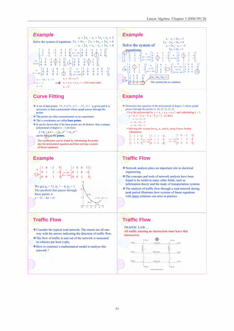
Linear Algebra- Chapter 3 20080926
53
ExampleExampleSolve the system of equationsSolve the system of equations
432636242232
54321
54321
54321
=+minus+minusminus=++minus+=++minus+
xxxxxxxxxxxxxxx
⎥⎥⎦
⎤
⎢⎢⎣
⎡ minusasymp
⎥⎥⎦
⎤
⎢⎢⎣
⎡
minusminusminusminusminus
+
minus+
642000210000213121
431121636242213121
R1R3
2)R1(R2
⎥⎥⎦
⎤
⎢⎢⎣
⎡ minusasympharr 210000
642000213121
R3R2 ( ) ⎥⎥⎦
⎤
⎢⎢⎣
⎡ minusasymp
210000321000213121
2R21
⎥⎥⎦
⎤
⎢⎢⎣
⎡ minusminusminusasympminus+ 210000
321000750121
3)R2(R1 ⎥⎥⎦
⎤
⎢⎢⎣
⎡minus
minusasymp
minus+
+
210000101000300121
2)R3(R2
5R3R1
2x1x
3xx2x
5
4
321
=minus=
++minus=rArr
2xs and r somefor 1x sx rx
3sr2x
5
432
1
=minus===
++minus=
ExampleExample
Solve the system of Solve the system of equationsequations 122
32452232
32
321
321
321
=+minus=minus+
=+minus=+minus
xxxxxxxxxxx
⎥⎥
⎦
⎤
⎢⎢
⎣
⎡asymp
minusminusminus
minus
harr1220210063303211
R3R2
( ) ⎥⎥
⎦
⎤
⎢⎢
⎣
⎡asymp
minusminusminus
minus
1220210021103211
R231
⎥⎥
⎦
⎤
⎢⎢
⎣
⎡asympminusminusminus
minus+
+
5400210021101101
2)R2(R4
R2R1 ⎥⎥
⎦
⎤
⎢⎢
⎣
⎡asymp
minusminus
minus+
+
minus+
13000210040103001
4)R3R(R4
R3R2
1)R3(R1
( ) ⎥⎥
⎦
⎤
⎢⎢
⎣
⎡asymp
minusminus
1000210040103001
R4131
The system has no solutionThe system has no solution
⎥⎥
⎦
⎤
⎢⎢
⎣
⎡asymp
⎥⎥
⎦
⎤
⎢⎢
⎣
⎡
minusminusminus
minus
minusminusminusminus
minus+
minus+
1220633021003211
1220312145223211
1)R1(R3
2)R1(R2
0x1+0x2+0x3=1
Curve FittingCurve Fitting
A set of data points A set of data points is given and it is is given and it is necessary to find a polynomial whose graph passes through the necessary to find a polynomial whose graph passes through the points points The points are often measurements in an experiment The points are often measurements in an experiment The xThe x--coordinates are called coordinates are called base pointsbase pointsIt can be shown that if the base points are all distinct then aIt can be shown that if the base points are all distinct then a unique unique polynomial of degree n polynomial of degree n ndashndash 1 (or less)1 (or less)
can be fitted to thecan be fitted to the pointspoints
) ( ) ( ) ( 2211 nn yxyxyx K
11
2210
minusminus
minusminus ++++= n
nn
n xaxaxaay K
The coefficients can be found by substituting the points The coefficients can be found by substituting the points into the polynomial equation and then solving a system into the polynomial equation and then solving a system of linear equationsof linear equations
ExampleExample
Determine the equation of the polynomial of degree 2 whose graphpasses through the points (1 6) (2 3) (3 2)
Let the polynomial be and substituting x = 1 y = 6 x = 2 y = 3 x = 3 y = 2 we have
Solving this system for a0 a1 and a2 using Gauss-Jordan elimination
⎥⎥⎥
⎦
⎤
⎢⎢⎢
⎣
⎡minus
minus
minus+minus+asymp
220033109201
1)R2(R31)R2(R1
2210 xaxaay ++=
2a9a3a3a4a2a6aaa
210
210
210
=++=++=++
⎥⎥⎥
⎦
⎤
⎢⎢⎢
⎣
⎡
minusminus
⎥⎥⎥
⎦
⎤
⎢⎢⎢
⎣
⎡
minus+minus+asymp
482033106111
293134216111
1)R1(R31)R1(R2
( )⎥⎥⎥
⎦
⎤
⎢⎢⎢
⎣
⎡minus
⎥⎥⎥
⎦
⎤
⎢⎢⎢
⎣
⎡minus
minusasymp
minus++asymp
11006010
11001
110033109201
3)R3(R22R3R1
R321
We get a0 = 11 a1 = ndash 6 a2 = 1The parabola that passes through these points is y = 11 ndash 6x + x2
ExampleExample Traffic FlowTraffic Flow
Network analysis plays an important role in electrical Network analysis plays an important role in electrical engineeringengineeringThe concepts and tools of network analysis have been The concepts and tools of network analysis have been found to be useful in many other fields such as found to be useful in many other fields such as information theory and the study of transportation systemsinformation theory and the study of transportation systemsThe analysis of traffic flow through a road network during The analysis of traffic flow through a road network during peak period illustrates how systems of linear equations peak period illustrates how systems of linear equations with with manymany solutions can arise in practicesolutions can arise in practice
Traffic FlowTraffic Flow
Consider the typical road network The streets are all oneConsider the typical road network The streets are all one--way with the arrows indicating the direction of traffic flowway with the arrows indicating the direction of traffic flowThe flow of traffic in and out of the network is measured The flow of traffic in and out of the network is measured in vehicles per hour (in vehicles per hour (vphvph))How to construct a mathematical model to analyze this How to construct a mathematical model to analyze this network network
Traffic Traffic FlowFlowTRAFFIC LAWTRAFFIC LAWhelliphellipAll traffic entering an intersection must leave that All traffic entering an intersection must leave that intersectionintersection
Linear Algebra- Chapter 3 20080926
54
Junction AJunction BJunction CJunction DJunction EJunction F 600
800 200 500 100 600
54
643
73
72
621
51
=+=++minus=+minus=minus=+minus=+
xxxxx
xxxx
xxxxx
⎥⎥⎥⎥⎥⎥⎥⎥⎥⎥⎥⎥⎥
⎦
⎤
⎢⎢⎢⎢⎢⎢⎢⎢⎢⎢⎢⎢⎢
⎣
⎡
asympasymp
⎥⎥⎥⎥⎥⎥⎥⎥⎥⎥⎥⎥⎥
⎦
⎤
⎢⎢⎢⎢⎢⎢⎢⎢⎢⎢⎢⎢⎢
⎣
⎡
minusminus
minusminusminusminus
minusminus
minusminus
0000000001110000
6001101000200100010050010000106001100001
600001100080001011002001000100500100001010001000116000010001
L
Traffic FlowTraffic FlowJunction AJunction BJunction CJunction DJunction EJunction F 600
800 200 500 100 600
54
643
73
72
621
51
=+=++minus=+minus=minus=+minus=+
xxxxx
xxxx
xxxxx
Perform road work on x7 Because x3 ge 0 the minimum flow 200 in the branch x7 can be obtained by making x3 = 0 (closing DE to traffic)
Traffic FlowTraffic Flow
We get
765
76473
72761
xx x600xxx200x x500x x600xxx
minus=++minus=minus=+=+minusminus=
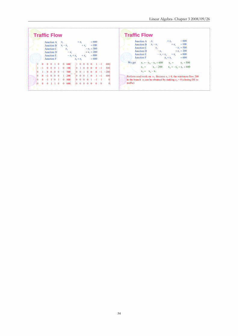
Linear Algebra- Chapter 3 20080926
54
Junction AJunction BJunction CJunction DJunction EJunction F 600
800 200 500 100 600
54
643
73
72
621
51
=+=++minus=+minus=minus=+minus=+
xxxxx
xxxx
xxxxx
⎥⎥⎥⎥⎥⎥⎥⎥⎥⎥⎥⎥⎥
⎦
⎤
⎢⎢⎢⎢⎢⎢⎢⎢⎢⎢⎢⎢⎢
⎣
⎡
asympasymp
⎥⎥⎥⎥⎥⎥⎥⎥⎥⎥⎥⎥⎥
⎦
⎤
⎢⎢⎢⎢⎢⎢⎢⎢⎢⎢⎢⎢⎢
⎣
⎡
minusminus
minusminusminusminus
minusminus
minusminus
0000000001110000
6001101000200100010050010000106001100001
600001100080001011002001000100500100001010001000116000010001
L
Traffic FlowTraffic FlowJunction AJunction BJunction CJunction DJunction EJunction F 600
800 200 500 100 600
54
643
73
72
621
51
=+=++minus=+minus=minus=+minus=+
xxxxx
xxxx
xxxxx
Perform road work on x7 Because x3 ge 0 the minimum flow 200 in the branch x7 can be obtained by making x3 = 0 (closing DE to traffic)
Traffic FlowTraffic Flow
We get
765
76473
72761
xx x600xxx200x x500x x600xxx
minus=++minus=minus=+=+minusminus=