chapter 3. · pdf fileengineering fieis manual chapter 3. hydraulics compiled by: william 5....

ENGINEERING FIEIS MANUAL

CHAPTER 3 . HYDRAULICS

Compiled by: W i l l i a m 5 . Urquhart, Civil Engineer, SCS, Portland, Oregon

Content 8

Page

General . . . . . . . . . . . . . . . . . . . . . . . . . . . . bmrersion of Units . . . . . . , . . . . . . . . . . . . , . . Hydrostatics . . . . . . . . . . . . . . . . . . . . . . . . .

Pressure-Deneity-Height Relationships . . . . . . . b . . . Piemmeter . . . . . . . . . . . . . . . . . . . . . . .

Forces on Submerged Plane Surfaces . . . . . . . . . . . . . Resaure Diagrams . . . . . . . . . . . . . . . . . . . .

Buoyancy and Flo ta t ion . . . . . . . . . . . . . . . . . . . Buoyancy . . . . . . . . . . . . . . . . . . . . . . . . F l o t a t i o n . . . . . . , . :. . . . . . . . . . . . . . .

Hydrokinetics . . . . . . . . . . . . . . . . . . , . . . . . . FlowContinuity . . . . . . , . . . . . . . . . . . . . . . Conservation of Energy . . . . . . . . . . . . . . . . . . .

Potential Energy . . . . . . . . , . . . . . . . , . . . Pressure Energy . . . . . . . . . . . . . . . . . . . . . Kinetic Energy . . . . . . . . . . . . . . . . . . . . . Bernoulli Principle . . . . . . . . . . . . . . . . . . . Hydraulic and Energy Gradients . . . . . . . . . . . . .

P i p e F l o w . . . . . . . . . . , . . . . . . . . . . . . . . . . Laminar and Turbulent Flaw . . . . . . . . . . . . . . . . .

F r i c t i o n L o s s . . . . . . . . . . . . . . . . . . . . . . Manning's Equation . . . . . . . . . . . . . . . . . . Haeen-Williams Equation . . . . . . . . . . . . . . .

Other Losses , . . . . . . . . . . . . . . . . . . . . . Hydraulics of Pipelines . . . . . . . . . , . . . . . . . Hydraulics of Culverts . . . . . . . . . . . . . . . . . . .

Culverts Flowing With I n l e t Control . . . . , . . . , . . . Culverts Flawing With Outlet Control . . . . . . . . . . Eroaive Culvert E x i t Velocit ies . . . . . . . . . . . . .

Open Channel Flow . . . . . . . . . . . . . . . . . . . . . . Types of Channel Flow . . . . . . . . . . . . . . , . . . .

3-1

3-1

3-3 3-3 3-4 3-5 3-7 3-10 3-11 3-11

3-14 3-15 3-16 3-16 3-16 3-16 3-18 3-18

3-19 3-19 3-19 3-20 3-21 3-23 3-23 3-30 3-30 3-33 3-37

3-37 3-38

Steady Flow and Unsteady Flow . . Uniform Flow and Nonuniform Flow .

Channel Croas-Section Elements . . . Manning's Equation . . . . . . . . .

Coefficient of Roughness. n . . . Physical Roughness . . . . . . . . Vegetation . . . . . . . . . . . . Cross Section . . . . . . . . . . Channel Alignment . . . . . . . . . S i l t i n g o r Scouring . . . . . . . Obstructions . . . . . . . . . . .

Speci f ic Energy i n Channels . . . . . C r i t i c a l Flaw Conditions . . . . . .

General Equation f o r Critical Flow Critical Discharge . . . . . . C r i t i c a l Depth . . . . . . . . C r i t i c a l Velocity . . . . . . . Critical Slope . . . . . . . . Subcr i t i ca l Flow . . I . . I . Superc r i t i ca l Flow . . . . . .

I n s t a b i l i t y of C r i t i c a l Flow . . . Open Channel Problems . . . . . .

. . . . . . . . . . . . . . . . . . . . . . . . . . . . . . . . . . . . . . . . . . . . . . . . . . . . . . . . . . . . . . . . . . . . . . . . . . . . . . . . . . . . . . . . . . . . . . . . . . . . . . . . . . . . . . . . . . . . . . . . . . . . . . . . . . . . . . . . . . . . . . . . . . . . . . . . . . . . . . . . . . . . . . . . . . . . . . . . . . . . . . . . . . . . . . . . . . . . . . . . . . . . . . . . . . . . . . . . . . . . Weir Flow . . . . . . . . . . . . . . . . . . . . . . . . .

Basic Equation . . . . . . . . . . . . . . . . . . . . . Contractions . . . . . . . . . . . . . . . . . . . . . . Velocity of Approach . . . . . . . . . . . . . . . . . . . Weir Coeff ic ien ts . . . . . . . . . . . . . . . . . . . . Submerged Flow . . . . . . . . . . . . . . . . . . . . .

WaterMeasuring . . . . . . . . . . . . . . . . . . . . . . Open Channels . . . . . . . . . . . . . . . . . . . . . .

Ori f i ces . . . . . . . . . . . . . . . . . . . . . . . Weirs . . . . . . . . . . . . . . . . . . . . . . . .

Rectangular Contracted Weir . . . . . . . . . . . . Rectangular Suppressed Weir . . . . . . . . . . . . C i p o l l e t t i Weir . . . . . . . . . . . . . . . . . . 900 V-Notch Weir . . . . . . . . . . . . . . . . .

Parsha l l Flume . . . . . . . . . . . . . . . . . . . . Trapezoidal Flume . . . . . . . . . . . . . . . . . . CurrentMeter . . . . . . . . . . . . . . . . . . . . Water-Stage Recorder . . . . . . . . . . . . . . . . . Measurements by F loa t s . . . . . . . . . . . . . . . . Slope-Area Method . . . . . . . . . . . . . . . . . . Velocity-Head Rod . . . . . . . . . . . . . . . . . .

PipeFlow . . . . . . . . . . . . . . . . . . . . . . . . Ori f i ceF low . . . . . . . . . . . . . . . . . . . . . Cal i forn ia Pipe Method . . . . . . . . . . . . . . . . Coordinate Method . . . . . . . . . . . . . . . . . .

Page

3-38 3-38 3-39 3-39 3-41 3-4 3-42 3-42 3-42 3-42 3-42 3-43 3-44 3-44 3-45 3-45 3745 3-45 3-45 3-45 3-46 3-47

3-49 3-50 3-51 3-51 3-51 3-51

3-52 3-52 3-52 3-54 3-56 3-56 3-58 3-59 3-60 3-61 3-61 3-63 3-64 3-65 3-65 3-66 3-66 3-68 3-69

Figures

Page

Figure 3-1 B Figure 3-2 Figure 3-3

Figure 3-4 Figure 3-5

Figure 3-6 Figure 3-7 Figure 3-8 Figure 3-9 Figure 3-10 Figure 3-11 Figure 3-12 Figure 3-13 Figure 3-14 Figure 3-15 Figure 3-16 Figure 3-17 Figure 3-18 Figure 3-19 Figure 3-20 Figure 3-21 Figure 3-22 Figure 3-23 Figure 3-24 B Figure 3-25 Figure 3-26

Figure 3-27 Figure 3-28 Figure 3-29 Figure 3-30

Figure 3-31

Relationship between pressure and head Piezometer tube i n a pipeline . . . . . . . . .

pressure l i n e s . . . . . . . . . . . . . . . . Pressure on submerged sur faces . . . . . . . . .

and open channel flow . . . . . . . . . . . . Pipe flow energy r e l a t i o n s h i p s . . . . . . . . . Culverts with inlet con t ro l . . . . . . . . . . Culverts with o u t l e t con t ro l . . . . . . . . . . Culvert water depth r e l a t i o n s h i p s . . . . . . . Various types of open-channel flow Channel energy r e l a t ionsh ips . . . . . . . . . . The s p e c i f i c energy diagram . . . . . . . . . . Sharp-crested w e i r . . . . . . . . . . . . . . . Broad-crested w e i r . . . . . . . . . . . . . . . Submerged weir . . . . . . . . . . . . . . . . . Flow through an o r i f i c e . . . . . . . . . . . . Submerged o r i f i c e . . . . . . . . . . . . . . . Types of weirs . . . . . . . . . . . . . . . . .

. . . . . Plo t t ing d i f f e r e n t i a l . l ength piezometer data i n the d e t e m i n a t i o n of equipoten t ia l

Relationship between energy forms i n pipe

. . . . . . .

P r o f i l e of a sharp-crested w e i r . . . . . . . . Rectangular contracted w e i r . . . . . . . . . . Suppressed weir i n a flume drop . . . . . . . . C i p o l l e t t i w e i r . . . . . . . . . . . . . . . . . 90° V-notch w e i r . . . . . . . . . . . . . . . . Parshall flume . . . . . . . . . . . . . . . . . Trapezoidal flume . . . . . . . . . . . . . . . Stage-discharge curve for unlined

i r r i g a t i o n canals . . . . . . . . . . . . . . Pipe o r i f i c e . . . . . . . . . . . . . . . . . . Ori f i ce c o e f f i c i e n t s . . . . . . . . . . . . . . Measuring f low by the Cal i fo rn ia pipe method . . Required measurements t o ob ta in flow

from v e r t i c a l pipes . . . . . . . . . . . . . Required measurements t o ob ta in f l a w

from hor i zon ta l pipes . . . . . . . . . . . . Tables

Table 3-1 Values of Manning's. n . . . . . . . . . . . . . Table 3-2 Values of Hazen-Williams C . . . . . . . . . . . Table 3-3 Entrance loss c o e f f i c i e n t s . . . . . . . . . . .

3-3 3-4

3-6 3-7

3-17 3-23 3-31 3-34 3-36 3 -44 3-43 3-45 3-49 3-50 3-50 3-52 3-54 3"54 3-55 3-56 3-57 3-58 3-59 3-60 3-62

3-64 3-66 3-67 3-68

3-69

3-70

3-22 3-22 3-35

Page

Ekhibit 3-1 Exhibit 3-2

Exhibit 3 -3 Exhibit 3-4

Exhibit 3 -5

m i b i t 3-6

Exhibit 3-7

Exhibit 3-8

Exhibit 3-9

Exhibit 3 . 10

Exhibit 3-11

Exhibit 3-12

Exhibit 3-13 Exhibit 3-14

Exhibit 3-15 Exhibft 3-16 M i b i t 3-17 Exhibit 3 . 18

Exhibit 3-19 Exhibit 3 -2 0

Water volume. weight and flow equivalente . Pressure diagrams and methods of computing

Required thickness of flashboards . . . . . Head loss c o e f f i c i e n t s for c i r c u l a r and

Discharge of c i r c u l a r pipes flowing f u l l . Solution of Hazen-Williams formula fo r

F r i c t i o n head l o s s i n semirigid p l a s t i c i r r i g a t i o n p ipe l ines . . . . . . . . . .

Head l o s s coef f ic ien ts fo r pipe entrances and bendaj . . . . . . . . . . . . . . . .

Headwater depth for concrete pipe cu lver t s with i n l e t control . . . . . . . . . . .

Headwater depth for CM pipe cu lver t s with i n l e t control . . . . . . . . . . . . . .

&ad fo r concrete pipe c u l v e r t s flowing f u l l with o u t l e t control . . . . . . . .

Head f o r CM pipe c u l v e r t s flowing f u l l with o u t l e t control . . . . . . . . . . .

Elements of channel sect ions . . . . . . . Solution of Manning's formula f o r

uniformflow . . . . . . . . . . . . . . Discharge f o r contracted rectangular weirs Discharge f o r C i p o l l e t t i weirs . . . . . . Discharge f o r 90' V-notch weirs

with f r e e discharge . . . . . . . . . . . Flow of water from vertical pipes Flaw of water from horizontal pipes

hydrostat ic loads . . . . . . . . . . . . square conduit8 flowing f u l l . . . . . . Manning's n . . . . . . . . . . . . . . . round pipes . . . . . . . . . . . . . . .

. . . . . . Discharge from c i r c u l a r pipe o r i f i c e s

. . . . . . . . .

0 . .

. . . . . .

. . . 0 . .

0 . .

0 . .

. . .

. . . 0 . .

. . . 0 . 0 . . . . . . . . . . . . . . . . . . . . . . . .

3-71

3-72 3-74

3-75

3-76

3-83

3-a4

3-89

3-91

3-32

3-93

3-34 3-95

3-96 3-100 3-103 3-106

3-107 3-108 3-109

ENGINEERING FIELD MANUAL

CHAPTER 3. HYDRAULICS

1. GENERAL

This chapter presents the hydraulic principles tha t apply t o the design and operation of s o i l and water conservation measures. help the technician to develop a be t te r understanding of hydraulics and t o use the equations and exhibits contained herein.

It w i l l

The chapter contains sections on conversion of units, principles of water a t rest (hydrostatics), and principles of water i n motion (hydrokinetics). It discusses the application of these principles t o the flow of water i n pipes, i n open channels, and through weirs. Lastly, the more common methods of measuring the flow of water i n open channels and pipes are covered.

2. CONVERSION OF UNITS

Valid equations must be expressed i n corresponding units. That is, i n a true equation there must be equality between both uni ts and numbers. The chance of making conversion errors can be greatly reduced by forming the habit of thinking i n terms of equality of units as w e l l as the i r r e l - a t ive numerical values.

The foot-pound-second system is used i n this chapter unless otherwise specified. Sometimes, however, it is necessary t o convert to other uni ts , which involves the use of numerical conversion constants. Some frequently used constants are given i n Exhibit 3-1.

EXAMPLE 3-1

It is desired t o build a stock water tank with a capacity i n cubic fee t that will contain one day's flow from a spring that flaws at the rate of three gallons per minute.

3 gallons per minute day 5 Y cubic feet

Since cubic f ee t can not be d i rec t ly equated t o gallons, some unit factor having numerical value must be introduced if the expression is t o be made a valid equation.

3 -2

The expression 3 gallons per minute per day is a f ract ional expression that can be written:

9 = 3 gal. __ 3 gal. - msal., min . day day

min . min , min . - - Analysis shows that :

Note that all units on the left cancel except cubic fee t , thus leaving the sane uni ts on each side of the equation. general equation f o r conversions between gallons per minute per day and cubic feet . 192,51 cu.ft. Then:

The resu l t i s the following

If 3 gal/mi’n/day equals 577.5 cu.ft., one gal/min/day equals

EXAMPLE 3-2

1 acre foot per hour = Y gallons per minute

Step by step analysis resu l t s i n a val id conversion equation consistent i n both units and dimenaions:

or

5431 gal. x s.H. min. =ygal.

min.

EXAMPLE 3-3

1 cubic foot per second day = Y acre feet

Anal y s i 8 r e su l t s in:

X- 1 ac. 43,560 9X.x-

X @ W x

2w x x = 1.9835 ac , f t .

1.9835 ac ft = y ac*ft* *

3 -3

I f t h i s approach t o conversion problems is used, the r e su l t s w i l l D be:

1. Freedom from conversion errors.

2. Savings in time i n both or iginal and "check" computations.

3. Accuracy of conversion factor select ion from standard tables and other sources.

3. HYDROSTATICS

The subject of hydrostatics ( f luid s t a t i c s ) deals with problems i n which the f lu id is motionless or a t rest.

PRESSURE-DENSITY-HEIGHT RELATIONSHIPS

The fundamental equation of f lu id statics r e l a t e s pressure, density, and depth. unit weight of the f lu id and are expressed by the equation:

Unit pressures i n a f lu id vary d i r ec t ly with the depth and the

p = w h or h = E W (Eq, 3-1)

where p = intensi ty of pressure per un i t of area w = un i t weight of the f lu id h = depth of submergence, or head.

Equation 3-1 shows t ha t pressure at any point i n a l iquid of given density depends solely upon the height of the l iquid above the point. This allows the ve r t i ca l height, or 'head," of the l iquid t o he used as an indication of pressure. "inches of mercury'' and "feet of water.'' The re la t ionship ef pressure and head is i l l u s t r a t ed numerically i n the 'hanometer" and ''piezometer columns" of Figure 3-1.

Thus, pressure may be quoted i n such uni t s as

co~umni

n

t 20.3d of

mercury L

7 23.1'

of water

Mercury

Figure 3-1 Relationshfp between pressure and he ad

3 -4

I f t h e tank i s f i l l e d with water u n t i l the pressure gage reads 10 p.s.i. , t he he ight of the water sur face i n the piezometers and the mercury i n the manometer can be ca l cu la t ed from Equation 3-1.

Example 3-4

10 lb . Water : h = 4 = 6::iiy;m x 144 sq.in. 23.3. feet

1 sq . f t . cU.ft.

Mercury (unit weight of 849 pounds per cubic foot ) :

10 Ib. h = sq.in.

cu . f t .

144 sq.in. x 12 in. = 20.35 inches 849 lb. 1 sq. f t . 1 f t .

Piezome ter

Figure 3-2 shows a piezmeter tube connected t o a pipe i n which the The height h l i s a measure of pressure at t h e liquid is unde,r pressureo

w a l l of the pipe i f t he opening is a t r i g h t angles t o the w a l l and f r e e of any roughness or pro jec t ion in to t h e moving l i q u i d . The pressure a t the w a l l of the pipe is: p1 = whl and t h a t a t the c e n t e r l i n e p = wh.

Figure 3-2 Piezometer tube in a p i p e l i n e

Piezometers a r e used to measure water pressure i n drainage inves t iga- tions and e a r t h dam foundation s tudies . r a t e d small-diameter pipe, so designed and i n s t a l l e d that a f t e r i t has been dr iven i n t o the s o i l the underground water cannot flow f r e e l y along the outs ide of the pipe and can en te r it only a t the bottom end. piezometer is so driven t h a t i t s lower end is i n t h e stratum o r a t the level where the pressure is t o be read. t he bottom of t he p ipe i s the pressure head.

Such a piezometer is an unperfo-

The

The he ight t h a t water rises above

3-5

A piezometer should not be confused with an observation w e l l which i s used t o determine the leve l of the water table . The w e l l permits water t o enter the hole a t any leve l , thus connecting t h e various water bearing strata i n the s o i l p r o f i l e . The properly i n s t a l l e d piezometer permits water t o en ter only a t the bottom end and from only t h a t l e v e l i n the s o i l p r o f i l e .

A typical example of the manner i n which piezometers of d i f f e r e n t lengths may be used i n sets t o determine whether a canal i s leaking i s i l l u s t r a t e d i n Figure 3-3. I n t h i s example, sets of four piezometers 5, 10, 15 and 20 feet i n length have been i n s t a l l e d on a l i n e a t r i g h t angles t o the axis of the canal a t dis tances of 15, 60, and 100 f e e t from the cen- t e r l i n e of the canal (Diagram A). The f i r s t object ive is t o obtain hydro- s ta t ic pressures a t a la rge number of points under the water t a b l e adjacent t o the canal.

In Diagram B, which represents the sane cross sec t ion shown i n A, the small circles indica te the pos i t ion of the bottom end of each piezometer. On the right-hand s ide of the sketch, the number beside each c i r c l e i s the water level elevat ion i n each piezometer. On the l e f t s ide the numbers are the elevat ions of the bottom ends of the piezometers. Note t h a t the water level elevat ions are greater than t h e elevat ions of the bottoms of the corresponding p i e z m e t e r s . The water surface elevat ion i n the piezometer is w r i t t e n a t the point i n the p r o f i l e where t h e bottom of the piezometer is located, not where the water surface i s located.

The t h i r d s tep i s t o draw contours of equal hydrostat ic pressures, as i n Diagram C. the same manner as ground surface contours are drawn i n the horizontal plane. Water moves through the s o i l f rom high t o l o w pressures and i n a d i r e c t i o n a t r i g h t angles t o the pressure contours. from the canal .

These pressure l i n e s are drawn i n the v e r t i c a l plane i n much

This example ind ica tes seepage

I f an a r t e s i a n pressure condition ex is ted i n the s o i l p r o f i l e , the deep piezometers would show higher water surface elevat ions than the shorter piezometers, and the ground water contours would indicate upward water pressure.

FORCES ON SUBMERGED PLANE SURFACES

The ca lcu la t ion of the s i z e , d i rec t ion , and loca t ion of the forces on submerged surfaces i s essential i n the design of dams, bulkheads, water cont ro l gates , etc.

3 -6 Assumed Elevation

(Feat) A

- 90

=< Ground Surface JJ.

Six batteries of differential - length pierorneters bracketing an irrigation canal and terminating at depths of 5,10,15,and 20 feet.

I

B

s5,0e

0 - 0 98.21 Q 95.91

0 0 9 0 0 0 97.50 0 95.80 0 95.00

0 0 - 0 85 0 96.72 0 95.75 0 94.05

l e s I I I I 80 -

0 0 w o 0 96.20 0 9550 0 94.70

The left side is plotted to show the piezometer terminotion levels. The pressures in the piezorneters are measured at these points. The right side gives the water elevations in the piexometsr tubes. These elevations are plotted at the piezometer termination points.

C

095.00

95.50 9620

The le f t side shows lines of equal pressure partly drawn. Lines of equal pressure are drawn sirnilor to ground -surface contoura. The right slde shows the finished lines of equal pressure and the orrow8 indicate the direction of ground- water movement.

190 8,0 6,O 4,O 2,O 0 2.0 4#0 6,O 8.0 lq0 Distance From Canal (Feet 1

Figure 3-3 P l o t t i n g differential-length piezometer data in the determination of equipotential pressure lines

3 -7

For a submerged hor izonta l plane, the c a l c u l a t i o n of u n i t and t o t a l pressures is simple because t h e pressure is uniform over the area. For v e r t i c a l and inc l ined planes the pressure v a r i e s with depth, as shown by Equation 3-1, producing the typ ica l p ressure diagrams and the r e s u l t a n t forces of Figure 3-4.

( FiwhA c.p. of A

c.a. of ~ressure - - 4 .&It prism x p = w h 2

2

Figure 3-4 Pressure on submerged surfaces

The shaded area, when mul t ip l ied by a u n i t of length equals volume, which is known as the "pressure volume," The r e s u l t a n t force , F, i s equal t o t he pressure volume and passes through i t s center of gravity (c.g.). The r e s u l t a n t force also passes through a po in t on the plane defined as the "center of pressure" (c.P.).

B- Pressure Diagrams

The analys is of s t ruc tu res under pressure usua l ly w i l l be s impl i f ied by use of pressure diagrams. head, diagrams showing the v a r i a t i o n of u n i t p ressure i n any plane take t h e form of t r i a n g l e s , trapezoids, or rec tangles .

Since u n i t p ressure varies d i r e c t l y with

I n solving problems of force due t o w a t e r p ressure , t h e magnitude, d i r ec t ion , and pos i t i on of the force must be considered. The t o t a l force represented by t he pressure diagram can, f o r some problems, be represented by a s ing le force arrow through the pressure center ac t ing i n the same d i r e c t i o n as the u n i t pressures.

Exhibit 3-2 gives the most commonly used pressure diagrams and methods of computing the hydros ta t ic load and center of pressure.

3 -8

Example 3-5 A flashboard type of dam is built with six 3 x 12-inch flashboards.

What i s (a) the load per foot on the bottom board, (b) the total load on the bottom board i f it i s six feet long, and ( c ) the load per foot on the top board ?

Solution: First draw the pressure diagram, remembering that a f in i shed 12-inch board is 11.5-inches or 0.96-foot wide.

Then from Equation 3-1:

p = wh = unit weight of water x depth of water

Pi = 62.4 (7.5) = 468.0 l b s . per sq. f t . p2 = 62.4 (7.5 - 0.96) = 408.1 lbs. per sq. ft.

pg = 62.4 (1.74 + 0 . 9 6 ) = 168.5 lbs. per sq. ft. p 4 = 62.4 (1.74) = 108.6 lbs. per sq. f t .

And from Figure 3-4 :

The hydrostatic load, F = whA = pA = unit preesure x area

then

(a) =

(c) =

The solution 8 truc ture .

468*0 +408m1 x 0.96 = 420.5 l b s . per f t . 2

420.5 (6) = 2523 lbs.

168*5 +108m6 x 0.96 = 133.0 l b s . per ft. 2

would be the same for 1 3 t o p l O g S in a water control

T

3-9

Example 3-6

36-inches wide by 24-inches high, and h l i s 9 f e e t ? What i s the t o t a l water load, F, on t h e headgate shown i f it is D Solution :

Pressure diagram of load on

Whl f Wh2 2 area F =

1 h

1 = 9 + 2 = 11 f e e t h2

F = 6 2 - 4 (’ ( 2 ) ( 3 ) = 3744 lbs.

Example 3-7

sec t ion of a co l l aps ib l e f l a sh - board with water a t t h e maximum allowable elevation. Determine the pos i t i on of the center of pressure and t h e p ivo t under the conditions shown. Experience has shown that the pivot on the ga t e must be 6/7 of t he d is tance , from t he bottom of t h e flashboard t o the center of pressure f o r t h e board t o co l lapse .

This sketch shows t h e c ros s

Solution :

p = W 2 2

Pressure Diagram

As defined, the center of pressure i s t h e point where a perpendicular through t h e cen te r of g rav i ty of t h e pressure prism s t r i k e s the area under pressure. Use Exhibit 3-2 for the so lu t ion of t h i s problem.

3-10

First draw the pressure diagram:

hl = 3 f t . and p1 = 62.4(3) = 187.2 lbs/sq.ft. = a

h2 = 3 + 6 = 9 and p2 9 62.4(9) = 561.6 lb s / sq . f t . = b

d = 6 ft.

then from Exhibit 3-2

I I - 2ad I- bd Y 3(a + b )

- - 2(187.2)(6) + 561.6(6) 3(187.2 f 561.6)

5616 .O 2246.6 2.50 ft. center of pressure

and

L = (2.5) = 2.14 f t . 7

Example 3-8

needed in a flashboard dam. of 7 f e e t , have a 6-foot span, and be of Coast Region Douglas Fir.

It i s required t o determine t h e m a x h u m thickness of flashboards The flashboards w i l l impound water t o a depth

This can be solved by t h e use of Exhibit 3-3.

From c h a r t A, thicknese = 3.40 inches From c h a r t B, co r r ec t ion = 1.15

Flashboard thickness = 3.4(1.15) = 3.91 inches U s e nominal 4 x 12-inch flashboards

BUOYANCY AM, FLOTATION

The familiar pr inc ip le8 of buoyancy and f l o t a t i o n are usua l ly s t a t e d , r e spec t ive ly :

1. A body submerged i n a f l u i d is buoyed up by a fo rce equal t o t he weight of f l u i d displaced by the body.

2. A f l o a t i n g body d i sp laces its own weight of t he f l u i d i n which it f l o a t s .

3-11

Buoyancy

A submerged body i s acted on by a v e r t i c a l , buoyant force equal t o the weight of the displaced water.

Fg = Vw (Eq. 3-2)

Fg = buoyant force V = volume of the body w = u n i t weight of water

I f the u n i t weight of the body is grea ter than t h a t of w a t e r , there is an unbalanced downward force equal t o the difference between the weight of the body and the weight of the water displaced. w i l l sink.

Therefore, the body

Flota t ion

If the body has a u n i t weight less than t h a t of water, the body will f l o a t with p a r t of i t s volume below and p a r t above the water surface i n a pos i t ion so t h a t :

w = v w (Eq. 3-3)

W = weight of the body V = volume of the body below the

water surface; i.e., the volume of the displaced water

w = u n i t weight of water

A check should be made of the s t a b i l i t y of hydraulic s t ruc tures as they w i l l be affected by submergence and whether the weight of the s t ruc- t u r e w i l l be adequate t o resist f l o t a t i o n .

Porous materials, when submerged, have d i f f e r e n t n e t weights depending upon whether the voids are f i l l e d with air or water. v a r i a t i o n i n the possible net weight of one cubic foot of t rea ted s t ruc- t u r a l timber weighing 55 pounds under average atmospheric moisture conditions and having 30 percent voids:

Note the wide

1 cu. f t . of s t r u c t u r a l Before After timber, 30 percent voids Saturat ion Saturation

W = weight i n a i r , lb. 55 55 + (0.30 x 6 2 . 4 ) = 73.72 FB = buoyant force when 62.4 62.4

submerged, l b . W-FB = weight when sub-

merged i n water (net weight), lb . 55 - 6 2 . 4 = -7 .4 73.72 - 62.4 = 11.32

3-12

Hater ia 1

T i m b e r Stone

The degree t o which the f a c t o r s discussed above are capable of a f f e c t i n g the ne t or s t a b i l i z i n g weight of a s t r u c t u r e is i l l u s t r a t e d by the following example:

Net Weights of Mater ia ls i n Founds per Cubic Yard of Dam

Not submerged Timber not saturated Timber saturated S ubrner ged

3.24 x 5 5 - 178 3 .21 (55 - 6 2 . 4 ) y -20 3 . 2 4 ( 7 3 - 6 2 . 0 - 34 1 6 . 6 3 x 150 p 2494 16.63(150 - 6 2 . 4 ) - 1457 1457

Example 3-9

under normal flood flows. Assume a timber crib diversion dam subject t o complete submergence

Materials, weights and volumes are:

Effec t ive or s t a b i t i e - ing weight of dam per 2672 c u b i c yard

Percent of Unit Weights Material Volume of the Dam lbs. /cu. f t .

1433 149 1

Timber Timber Loose stone, 30 percent voids

12

88

55 in air 73 saturated 150 s o l i d stone

Determine the ne t weight of one cubic yard of the dam when 1) not submerged, 2 ) submerged but timber not saturated, and 3) submerged with timber saturated,

1. Compute cubic feet of timber, s o l i d stone, and voids per cubic yard of dam:

a. Timber 0.12 x 27 = 3.24 CU. f t . b. Solid stone 0.7 x 0.88 x 27 = 16.63 cu. f t . c. Voids 0.3 x 0.88 x 27 = 7.13 CU. ft.

2 . Compute the n e t weights of one cubic yard of dam:

3-13

Example 3-10

be constructed. Determine i f it i s safe from f lo t a t ion with a safety fac tor of 1.5 and i f not, determine the size of spread footing required. follows :

A box i n l e t drop spillway for a 4 x &foot highway culver t is t o The box i n l e t has been designed as shown.

Design assumptions are as

D 1. The soil is saturated t o the l i p of the box and has

a buoyant weight of 50 pounds per cubic 'foot.

2. There is no f r i c t i o n a l res i s tance between the w a l l s of the box and the surrounding soil.

3 . Unit weight of concrete - 150 pounds per cubic foot,

4. Unit weight of water - 62.4 pounds per cubic foot.

F i r s t determine the weight (W) of the box.

End w a l l = 4' x 4' x 0.67' x 150

2 sidewalls = 4' x 8.67' x 0.67' x 150 x 2 - Floor s lab = 5.33 x 8.67 x 0.75 x 150

= 1,608 lba.

6,907 - 5 ,199

W - 13,714 lba.

3-14

Next determine the buoyant fo rce (FB) ac t ing on the box by

FB = Vw = (5.33 x 4.75 x 8.67) 62.4 = 13,697 l b s .

kom Equation 3-3, flotation w i l l occur i f W is less than or equal (FB has been subs t i t u t ed from Equation 3-2 f o r Vw):

Equation 3 -2 :

to FB

13,714 lbs . is grea te r than 13,697 lbs., therefore , the box will not float, but t h e required s a f e t y f a c t o r of 1.5 has not been accomplished.

bquired weight of box: W = 1.5 FB = 1.5(13,697) = 20,546 l b s .

Additional weight t o be added to box = 20,546 - 13,714 = 6,832 l b s .

This add i t iona l weight w i l l be provided with a spread foot ing around th ree s ides of t h e box, and t h e weight of the e a r t h load on t he footing.

J7%FsT Weight per square foo t of spread foot ing

b u y a n t soil f 50 ItUcu. ft.

= w, -I- w, -

= 200 -t- 65.7 = 265.7 lbs. t

Required area of foot ing 7

= - - 6832 - 25.7 sq. f t . 265.7

I

wCOllC

I f a one f o o t wide spread foot ing is provided, the foot ing area would be 2(8.67) + 7,33 = 24.7 sq. f t . and provide 24.7(265.7) = 6550 lbs. of add i t iona l weight. The safety f a c t o r aga ins t u p l i f t would be:

13,714 + 6550 = 1,48 13,697 SF =

Similarly, a spread foot ing 1'-3"wide would produce a s a f e t y factor of 1.57. By i n t e rpo la t ion , a foot ing 1'-1" wide would meet the f a c t o r of s a f e t y requirement.

4 . HYDROKINETICS

Hydrokinetics is the solution of f l u i d problems i n which a change of motion occurs as t he r e s u l t of the appl ica t ion of a force to t h e f l u i d body (water i n motion).

3-15

pukl CONTINUITY

When the discharge through a given cross section of a channel or pipe is constant, the flow i e steady. tions i n a reach, the flow is continuous. This ie known as continuity of flow and is expressed by the equation:

I f steady flow occure at a l l sec-

Q = a l v l = a2v2 = a3v3 - %vn (Eq. 3 - 4 )

where Q a discharge i n cubic feet per second a = cross-sectional area i n square f e e t v - mean veloci ty of flow i n f e e t per second 1, 2, 3, n = subscripts denoting d i f fe ren t cross sec tions

Most of the hydraulic problems handled by f i e l d technicianr deal with cases of continuous flow.

10 cfs of water flows through the tapered pipe ah- below. Calcu- late the average ve loc i t ies at eectione 1 and 2 with dismeters of 16 and 8 inches respectively.

from Equation 3-4

16 where d , in feet, equals 12 A a16 E d 2

4

= 7.16 fps 10 10 = 3.1416(1.333)?

4

3-16

Similarly :

v* = e = 10 = 20.64 fpe a

or, based on the r a t i o of crose-sectional areas

V8 - V16(?? = 7.16&y - 28.64 fps

CONSERVATION OF ENERGY

Three forms of energy are normally conaidered i n the analysis of problems i n water flow: and kine t ic energy.

Potential or elevation energy, pressure energy,

Potential Enerav

Potential energy is the a b i l i t y t o do work because of the elevation of a ma88 of water with respect t o some da tm. an elevation e feet, has potent ia l energy mounting t o ws foot pounds with respect t o the datum. quantity i n f ee t , but a l so energy i n foot pounds per pound.

A mas8 of weight, w, a t

The elevation head, e, expresses not only a l inear

Ressure Enerm

Rsaeure energy i r acquired by contact w i t h other masses and is A mass

Pressure energy may tranmnitted t o or through the l iquid mas8 under consideration. of water, aa such, does not have preesure energy. be supplied by a preesure pump or through same other applied force. pressure head (h - 2) a160 expresses energy in foot pounds per pound.

Kinetic E n e r a

The

W

Kinetic energy exista because of a veloci ty of motion and amounts to:

where W - weight of the water v = veloci ty i n f e e t per second g = acceleration due t o gravi ty

When W equals one pound, the kinetic energy has a value of 2. 2g

3-17

This expression i a cal led the velocity head. velocity of a stream of water is kn&, it , is poaeible t o compute the head which is converted from presaure energy o r potent ia l energy t o create kinet ic energy, This pr inciple is extremely important i n hydraulics.

In other word@, if the

Under ce r t a in conditions, the three forms of energy are interchange- able. channel flow is ehmm by Figure 3-5.

The relat ionship between the three forme of energy i n pipe and

Figure 3-5 Relationehip between energy forms in pipe and open channel flow

The t o t a l head, HI, is a vertical distance and represents the value of the t o t a l energy i n the eystem a t Section 1. velocity head which is equivalent t o the kine t ic energy, the preseure head which is equivalent t o the energy due t o pressure, and the elevation head which is equivalent to the energy due t o poeition.

This is made up of the

In the case of channel f l w , the veloci ty head is the difference in elevation between the energy line and the water surface.

In the case of pipe f lou, the veloci ty head is the difference between

In pipe flow the pipe may be lowered or ra ised the elevation of the energy line end the elevation t o which water would rise in a pieeometer tube. within the zone of the elevation and the pressure heads without changing the conditions of flow. I f the entrance end of the pipe is lowered, the elevation head is reduced, but the preeswe head is increased a corresponding amount. Conversely, i f the entrance end of the p ipe i a raised, the elevation head is increased and the pressure head is decreased. If the quantity of flaw and dirrmeter of pipe did not change, then the velocl ty head w i l l remain the s a m .

3-18

Bernoul 1 i Pr inc i p le

Bernoulli 's pr inciple is the application of the l a w of conservation of energy t o f l u i d flow. It may be s ta ted as follows: In f r i c t i o n l e s s flow, the sum of the k ine t ic energy, pressure energy, and elevat ion energy i a equal at a l l sect ions along the stream, This means tha t if w e meaeured the veloci ty head, the pressure head, and the e levat ion head a t one eta- t i on i n a pipe or open channel carrying flowing water without f r i c t i o n , we would f ind t h a t the t o t a l would be equal t o the t o t a l of the ve loc i ty head, the pressure head, and the elevation head a t a second s t a t ion downstream in the same pipe or open channel, Figure 3-5. the pr inciple is used t o work out practical solutions. tion and all other energy loseee must be considered and the energy equation becomes :

This is theore t ica l , but In pract ice , fric-

where v = mean ve loc i ty of flow p = u n i t pressure w = un i t weight of water g - accelerat ion of gravi ty z = elevat ion head

h g

sub 1, "8

= all losses of head other than by f r i c t i o n between

= head loss by f r i c t i o n between Stations 1 and 2 Stations 1 and 2 such as bends

denotes upstream and downstream s t a t ions , respectively

The energy equation and the equation of continuity (Q = a1 v1 = a2 v2) are the two basic, simultaneous equations used i n solving problems i n water flow.

Hydraulic and EnerEy Gradients

The hydraulic gradient i n open-channel flow is the water surface, and i n pipe flow it connects the elevations t o which the water would rise i n piezmneter tubes along the pipe. !Che energy gradient is above the hydrau- l i c gradient, a distance equal t o the ve loc i ty head. In both open-channel and pipe flow, the f a l l (or slope) of the energy gradient for a given length 'of channel or pipe represents the lo s s of energy by friction. When considered together, the hydraulic gradient and the energy gradient r e f l e c t not only the loss of energy by f r i c t i o n , but also the conversions between the three forms of energy. See Figure 3-5.

3-19

5. PIPE F W

Pipe flow exiets when a closed conduit of any form is flowing f u l l . In pipe flow, the crose-sectional area of flow is fixed by the cross section of the conduit and the water surface is not exposed t o the atmosphere. than, or lees than the local atmospheric pressure.

Ihe internal pressure within a pipe may be equal to , greater

The principles of pipe flow apply t o the hydraulice of such struc- tures as culverts, drop in l e t s , regular and inverted siphons and various types of pipelines .

The concept of flow continuity and the Bernoulli principle has been discussed i n the preceding section. turbulent flcw, diecueses the commnly used diecharge equations and out- lines the hydraulics of pipelines and culverts.

This section defines laminar and

Water flmre with two different types of motion, laminar and turbulent.

Laminar flow occurs when the individual p8rtiC186 of water move in para l l e l layers. same. of the hydraulic gradient.

The veloci t ies of theae layers are not necessarily the However, the mean velocity of flow varier d i rec t ly with the slope

Turbulent flow i e an irregular type of flow i n which the par t ic les follow unpredictable paths. t ion of flaw, there are transverse components of velocity. The mean veloc i ty of flow varies with the square root of the slope of the hydraulic gradient .

In addition t o the main velocity i n the direc-

Laminar flow ee ldm occurs i n pipe flow. It is the type of flow that water has through so i l s . For pipe flow the motion is turbulent.

Fr ic t ion Loss

The loss of energy or head resul t ing from turbulence created at the boundary between the sides of the conduit and the flowing water is called f r i c t ion loss.

In a st ra ight length of conduit, flowing f u l l , with constant cross section and uniform roughnesa, the rate of loss of head by f r i c t ion is constant and the energy gradient has a slope i n the direction of flow equal t o the f r i c t ion head loss per foot of conduit.

3-20

Of the many equations that have been developed to expreaa this lose of head, the following two are the moat widely used:

MannlnR'r Equation The general form of Manning's equation is:

(Eq. 3-6)

with the following nomenclature:

a - cross-eectional area of flow in ft. 2 - acceleration of gravity - 32.2 ft. per Bec. 2 d - dimeter of pipe in feet

d i = dimeter of pipe in inchea g Hi lose of head in feet due to friction in length, L K,= % = L " n = P = r -

I '

v = Q =

head lose coefficient for any conduit head lose coefficient for circular pipe length of conduit in feet Manning's roughneaa coefficient wetted perimeter in feet hydraulic radius in feet = g - d for round pipe

lone of head in feet per foot of conduit = slope of energy grade and hydraulic gradelinee in straight conduits of uniform croee section mean velocity of flow in ft. per eec. discharge or capacity In cu.ft. per eec.

P Z

(H1+L)

Starting with Equation 3-6 solve fox s, multiply numerator and de- nominator of right side of equation by 2g and substitute (Hi+L) for IS. The result ia :

29.164 n2 L V2 2g = 413

H1

ihe equation can be simplified by substituting

29.164 n2 r 413 KC

then the equation talces the form

(Eq. 3-7)

3-21

Maption of Equation 3-7 to circular pipes iuvolver the uubs t i tu tbn of (d + 4) for r 4 the change frm d t o d i . B

Tables for values of 5 and given in Jhhibit 3 4 0

King's Eandbook(l) glvea a mnnber of convenient working form of llarming'e formula a d references t o tables that w i l l f a c i l i t a t e theix ume. Four of these are:

for the usual ranger of variable0 are

B Exhibit 3-5, which is baeed on the last of these equations, -be used t o determine d i , 8 , or Q when two of them quant i t ieo a d n are -. Values of Manning'e n are given in Table 3-1.

€la%en-Willima Eauation As generally used, t h i s equation I s :

v = 1.318 C rO.63 s 0 - s (Eq. 3-10)

Notation is the 6- as given fole Manning'e equation with the addi- t ion of C, the coefficient of roughneae in Hazen-Williams formula.

Since Q av, Equation 3-10 may be converted t o the follwing foemula for discharge in any conduit:

Q - 1.318 a C r 0.63

Substitution of a a d r - in terma of inside diameter of plpe i n incheo in t h i s equation gives the follming general formula for discharge in c i r - cular pipee:

Q / C - 0.0006273 d12*43 (Eq. 3-11)

3-22

Values of n Min . Desinn Max. Desar ipt ion of pipe

Cast-iron, coated 0.010 0.012 - 0.014 0.014 Cast-iron, uncoated 0.011 0.013 - 0.015 0.015 Wrought iron, galvanized 0.013 0.015 - 0.017 0.017 Wrought iron, black 0.012 0.015 Steel, riveted and apiral 0.013 0.015 - 0.017 0.017

Helical corrugated metal 0.013 0.015 - 0.020 0.021 Wood stave 0.010 0.012 - 0.013 0.014 Nest cement surface 0.010 0 . 013 Concrete 0.010 0.012 - 0.017 0.017 Vitrif ied sewer pipe 0.010 0.013 - 0.015 0.017 Clay, camon drainage t i l e 0.011 0.012 - 0.014 0.017

I Corrugated plast ic 1 0.014 0.015 - 0.016 0.017

I Annular corrugated metal 0,021 0.021 0 0.025 0.0255

Graphical solutions of Equation 3-11 for standard pipe ranging frcm 1 to 12 inches in diameter and a wide range i n elope may be made by using Exhibit 3-6. Exhib i t 3-7 gives loaaes for aemi-rigid p las t ic pipe.

Values for C for different types of pipe are given i n Table 3-2.

I

I

Rsgardlesa of the designer's preference of equatione, the resu l t s ahould be checked against the application of State deeign c r i t e r i a .

3 -23

Other Losses

In addition t o the f r i c t i o n head losses, there are other losses of energy which occur as the r e s u l t of turbulence created by changes i n ve- l oc i ty and di rec t ion of flow. energy equation, such losses are commonly expressed i n terms of the mean veloci ty head a t sane spec i f ic cross sect ion of the pipe.

To f a c i l i t a t e t h e i r inclusion i n Bernoulli's

These loeses are sanetimes called minor loeses, which may be a serious

Such misnomer. only a mall p a r t of the t o t a l loss and i n such cases can be ignored. is not the case i n many s t ructures such aa culver ts , drop inlets, and si- phone which are r e l a t ive ly short . Safe design pract ice requires an estimate of such losses. If the estimate indicates t ha t minor losses amount t o 5 percent or umre of the t o t a l head loss, they should be careful ly evaluated and included in the flow calculations.

In long pipelines, the entrance loss, bend losaee, e tc . , may be

As velocities increase, careful determination of euch minor losses bec-8 more important. neglect of an entrance lose of 0.5 v2/2g results i n an error in head loss of 7 fee t . Whereas, i f the mean veloci ty is 3 feet per second, neglect of euch an entrance loss results in an error of only 0-07 foot.

With a mean veloci ty of 30 f e e t per second, the

Data on minor losses most commonly required are contained i n Exhibit 3-8 of t h i s chapter, and Section 5, Hydraulics, (6) and Section 15, Irriga- tion, of the National Engineering Handbook.

The pipe flow condition of ten found i n SCS work is t ha t of f r ee flw discharge. See Figure 3-6.

3 -24

The general pipe flow equation is derived through use of the

Equating the energy in Figure 3-6, using Equation 3-5:

Bernoulli and continuity principles.

where '1 = elevation head at station 1

= elevation head at etation 2

= velocity head at station 2

= s m of the minor head losses and pipe friction

=2

v2

ZK'J'J 2g 1 0 8 B e R

bt H I ti - "2

or

and fran the continuity principle

where Q = diecharge-cfs 2 a - pipe area-sq.ft.

g - acceleration of gravity-ftlsec. H = elevation head differential-ft.

= coefficient of minor losses Kp - pipe friction coefficient L - pipe length-ft.

3-25

The follwing e-lee are applications of Equation 3-12.

Example 3-12 D Determine the diecharge of a drop inlet epillway with cantilevered

The epillway is 24-inch di-ter rein- outlet for a head B of 20 feet. forced concrete pipe with Manning's n of 0.013, Table 3-1. for bend and entrance lorreem.

is 1.0 See refereme, sheet 2 of Exhibit 3-8.

I- 100'

So 1 ut ion

Uiing equation (3-12)

1. Area Reference: Exhibit 3-4

a = 3.14 EQ f t

2. Friction loss coeff ic ient Reference: Exhibi t 3-4

5 - 0.0124

3. Discharge

Q - 3.14 -(- 1+1+(0.0124) (100)

3-26

=ample 3-13

A corrugated metal pipe with a hooded inlet: and cantilevered outlet is t o discharge 130 cfs when the reservoir water surface i s at elevation 200.0 and the centerline of the outlet i a at elevation 170.0. Determine the diameter of pipe required. Use Manning's n = 0.024, Table 3-1.

Solution

Select a d i m e t e r and determine the discharge using Equation 3-12.

Trial 1

1. Select d = 36 inches

2. Area Reference: Exhibit 3-4

a - 7.07 eq.ft.

3. Friction 1066 coefficient Reference: Exhibit 3-4 5 = 0.0246

4. Minor loss coefficient Reference : Exhibit 3-8 (b=b%=&+O=K,)

entrance = 1.00

5 . Discharge

Q - 138.0 cfs

8

3-27

Trial 2

I. Select d = 30 inches

2 . Area a = 4.91 eq.ft.

3. Friction lose coefficient 5 0.0314

4. Minor lose coefficient % = 1.00

5 . Diecharge

Q = 4.91 2 ) (32.2) (200-170)

It can be seen frau the foregoing two trials that the 36-inch pipe more nearly sa t ie f iee the required Q of 130 cfe and is the one t o be installed.

Exrrmple 3-14

An 8-inch diameter concrete side drain in le t diechargee belcw the water surface of a channel. The pipe is 40 fee t long and flowing full with a head of 5 feet. Manning'e n = 0.012, Table 3-1. Determine the discharge. Aserne - entrance coefficient plus bend coefficient = 1.B

The discharge equation for exit conditions other than f ree flow i 8 the same as Equation 3-12.

K = exit coefficient = 1.0 X

3-28

theref ore I

1. Area Reference : Exhibit 3-4

a = 0.349 eq.ft.

2 . Friction loss coefficient Reference: Ekhibit 3-45 - 0.0458

3. Discharge t

(2) (32.2) (5)Q = 0.349 ,/ l + l + ( O .W58) (40)

A pipel ine of 250 feet of 36-inch and 500 feet of 24-inch steel pipe connects hpo rerervoirs. Determine the dimcharge i f : the head ie 100 feet, the entrance coefficient is 1, the contraction coefficient ie 0.25, and Manning's n is 0.011.

250' 500' -

To use Equation 3-12 the loas coefficients must be expressed i n terms of a single-sized pipe.

In terms of the 24-inch pipe the coefficients in the example must be multiplied by the follcwing ratio, C, which is based on the square of the ratio of areas.

3-29

rea of 24" dia. .'36 ere, of 36" dia . pipe

$4 - of 24" dia . p ips of 24" dia.pipe

Discharge in terme of 24-inch diameter pipe

1.. Areas Reference: Exhibit 3-4

24-inch d ia . a = 3.14 eq.ft. 36-inch d ia . a - 7.07 6q.ft.

2 . Friction lose coefficients Reference: Exhibit 3-4

24-inch dia . 5 - 0.00889 36-inch dia . $ = 0.00518

3. Square of the ratio of area8

3 14 - 0.196 c36 =

4. Sum of the loss coefficients

Item

Entrance 36" pipe Contraction 24" pipe~-Exit

AdjL L K C loae

- - 1.0 0.196 0.196 0.00518 - - 0.25 0.196 0.049 0.00889 500 4.45 1.0 4.45

e " 1.0 1.0 1.0

5.949

250 1.296 0.196 0.254

5. Discharge

103 cfe

3-30

HYDRAULICS OF CULVERTS(2)

There are two major types of culver t flaw: 1) Flow with i n l e t cont r o l , and 2 ) flm with ou t l e t control. For each type, d i f f e ren t factors and formulaa are used t o compute the hydraulic capacity of the culver t . Under inlet control, the slope, roughness and diameter of the culver t barrel , the i n l e t shape and the amount of headwater or ponding at the entrance must be considered. Outlet control involves the additional consideration of t he elevation of the tailwater i n the ou t l e t channel and the length of the culvert .

The need for making involved computations t o detemLne the probable type of flow under which a culver t w i l l operate may be avoided by computing headwater depths fran &hib i t s 3-9 through 3-12 for both inlet control and ou t l e t control and then using the higher value fo r design.

Both i n l e t control and ou t l e t control types of flow are diecussed briefly i n the following paragraphs.

Culverts Flowing With Inlet Control

Inlet control means that the discharge capacity of a culver t I s con-t ro l l ed at the culver t entrance by the depth of headwater. (m) and the shape of the entrance. Figure 3-7 shows i n l e t control flcw for three types of culver t entrances.

In i n l e t control the length of the culver t bar re l and ou t l e t condit ions are not fac tors i n determining culver t capacity.

In a l l culver t design, headwater or depth of ponding a t the entrance t o a culver t is an important factor i n culver t capacity. Thqheadwater depth is the ve r t i ca l distance from the culver t invert a t the entrance t o the energy l i n e of the headwater pool (depth + v e l o c i t y head). Because of the low veloc i t ies i n most entrance pools, the water surface and the energy l i n e at the entrance are assumed t o coincide.

Headwater-discharge relat ionships for various types of c i r cu la r culverts flawing with i n l e t control are baaed on laboratory research with models and ver i f ied in some instances by fu l l - sca le t e a t s . Exhibits 3-9 and 3-10 give headwater-discharge relationehipa for round concrete and CM pipe culver ts flowing with i n l e t control.

Example 3-16 It is desired to determine the m a x i m u m discharge of an exis t ing

42-inch concrete culvert . The allowable headwater depth (HW) upstream i e 8.0 f e e t and the slope of the culver t i s 0.02 f t / f t . The culver t has a projecting entrance condition and there w i l l be no backwater from downetream flow. Assume inlet control.

------

3-31

Figure 3-7 Culverts w i t h inlet control

D

3-32

Ueing Exhibit 3-9, cumpute D

At 2.29 on ecale 3, projecting entrance, draw a horizontal l i ne t o ecale 1. From th i s point on scale 1 draw a connecting line between it a d 42-inch diameter w scale 4. Ch ecale 5 read Q - 128 cfs.

Check for i n l e t control

where

> = symbol for "is greater than"

so - installed rlope of culvert

en = neutral elope - that elope of which the lose of head dua t o f r i c t ion i a equal t o the gainin head due t o elevation.

from Table 3-1, n(desiga) for concrete pipe - 0.012

frw m i b i t 3-5, mheet 3 of 6

for Q = 128 cfr a d D - 42 inchee

sn = 0.013

therefore, the culvert is in i n l e t control, 0.02 >0.013

Examle 3-17 Determine the required dimeter of a corrugated metal culvert pipe t o

be installed i n an existing channel. Q = 100 cfs, Ew max. = 7.0 f ee t and a0 = 0.03. There w i l l be no bacbater from downstream flm. Entrance t o be mitered t o conform to the alope of the embankment.

The solution of th i s problem must be made by tr ial pipe dimnetere and eolution of fw by uae of Exhibit 3-10.

Try D = 36"

draw a l i n e thrwgh 36 inch on scale 4 and 100 cfe on 8 C a b 5 to an intereection with ecale 1, then a horizontal line from wale I t o scale 2 , mitered in le t . On scale 2 read €iW- 3.8,

then €El - 3.8(3) - 11.4 feet too high

3-33

Try D = 48"

read from scale 2 ,

HW = 1.45(4) = 5.80

Try D = 42"

read from rcale 2,

-tw = 1.45 D

f e e t

HwD= 2.23

HW = 2.23(3.5) - 7.8 f e e t high

From the foregoing t r ia ls , it w i l l be necessary t o i n e t a l l the 48-inch diameter pipe i f the Hw is t o be 7.0 feet maximum.

Check f o r inlet control

from Exhibit 3-5, eheet 6 of 6

0.03 > 0.017 therefore , i n l e t control

Culverts Flowing With Outlet Control

Culverts flowing with o u t l e t control can flaw with the cu lver t b a r r e l f u l l fox a l l or p a r t of the b a r r e l length. See Figure 3-8. If the e n t i r e cross sect ion of the barrel i s f i l l e d with water f o r the t o t a l length of the b a r r e l , the cu lver t is sa id t o be i n f u l l flbw, Figure 3 - 8 ( a ) and (b). One other type of o u t l e t control is shown i n Figure 3-8(c). For this condition, the e levat ion of the energy gradeline a t the exit of the cu lver t is assumed a t 3 /4D. This is not an exact f igure but it w i l l give reasonable r e s u l t s .

The head, H, Figure 3-8(a), or energy required t o pass a given quant i t y of water through a culver t with o u t l e t control i s made up of th ree p a r t s . The p a r t s are expressed i n f e e t of water and include a veloc i ty head, h,an entrance loss, H,, and a f r i c t i o n loas, Hf. This energy is obtained from ponding of water a t the entrance and i s expressed by the equation

H = yT + H, f Hf (Eq. 3-13)

This equation i n similar form has been derived in the sec t ion on Hydraulics of pipel ines .

The entrance loss, He, depende upon the shape of the i n l e t edge. This l o s s i s expressed as a coef f ic ien t , %, times the b a r r e l velocity head. That is , I& = & v2 Entrance l o s s coef f ic ien ts , &, for various types of

E* entrances when flow is i n o u t l e t control are given i n Table 3-3.

3-34

Figure 3-8 Culvert8 with outlet control

- - - - - - - - - - - - - - - - - - - - - - - - - - - -

- - - - - - - - - - - - -

3-35

B Table 3-3 Entrance Lose Coefficients

Type of Structure and Design of Entrance Coefficient Ke r

Pipe, or Pipe-Arch,Corrugated Metal

Projecting ftm fill (no headwall)- - 0.9 Headwall or headwall and wingwalle

square-edge- I - I - - - I I - 0.5 Mitered t o conform to fill slope - - - - - 0.7 *End-section conforming t o fill slope - - 0.5

Note: *"End-section conforming t o fill slope,"made of either metal or I concrete, are the sections commonly available fran manufacturers.

From l imited hydraulic teats they are equivalent in operation t oj a headwall in both inlet and outlet control.

The friction loss, Hf, is the energy required t o overcane the roughness of the culvert barrel and is expressed by the equation

E$ values can be taken frun Exhibit 3-4.

Headwater depth can be expressed as an equation for a l l outlet control conditions, including a l l depths of tailwater, W. This is done by designating the vertical distance from the culvert invert at the outlet to the elevation from which H is measured as ho.

3-36

where B - length of cu lve r t so = elope of c u l v e r t in feet per foot H - head 1088 in feet as determined from t he

appropriate exhibit

When the e l eva t ion of the water rurface i n the o u t l e t channel is equal t o or above the top of the c u l v e r t opening a t t he o u t l e t , Figure 3-9(a) , h, i r equal t o the tailwater depth. If the tailwater e leva t ion is belw the top of the c u l v e r t opening at the o u t l e t , Figure 3-9(b) , h,, is then by definition 3/4D.

t - 1-1

Figure 3-9 Culvmrt mter dmpth ra,latlonrhipe

Headwater-diecharge relationships for varioue types of circular cul verts flowing with outlet cont ro l may be solved by the use of Exhibits 3-11 and 3-12. For a different roughneem c o e f f i c i e n t n1 than t h a t of the exh ib i t n, use the length aca les ehovn with an adjusted length, a, , calculated by the formula

3-37

Example 3-18 It is desired t o i n s t a l l 50 f e e t of concrete culver t p ipe , 'n - 0.012,

i n a drainage channel for a road croseing. Design Q i e 80 c f r with B tailwater depth of 3.0 fee t . Slope of the culver t w i l l be 0.002 foot per foot. Maximum headwater depth (HW) is 5 f ee t .

from Equation 3-14 IW = H +h, - a0a or, H - IW - ho + sol H = 5.0 - 3.0 + .002(50) H = 2.1 f e e t

and from Table 3-3 for a concrete pipe projecting from the f i l l with socket: end upstreamK, 0.2

entering Exhibit 3-11 draw a l i n e between H = 2.1 feet on the head ecale and Q = 80 cfs on the discharge ecale. Then on the length sca le for K, = 0.2, draw a second l i n e from the 50-feet mark through the intersect ion of the f i r s t line with the "turning l ine" and on t o the pipe diameter scale. The diameter scale intersect ion is a t approximately 39 inches, therefore, use a 42-inch pipe.

Erosive Culvert Exit Velocitiee

A culver t , becauee of its hydraulic charac te r i s t ics , increases the veloci ty of flow over tha t i n the adjacent channel. High ve loc i t ies may be damaging just downstream from the culver t ou t l e t and the erosion potent ia l at t h i s point should be considered i n culver t design. In many cases it is necessary t o r iprap the channel for a short distance doumstremn of the culver t exit.

6 . OPEN CHANNEL FLW

The flaw of water i n an open channel d i f f e r s from pipe flow in one important respect. See Figure 3-5. Open channel flm must have a free water 8urface, whereas pipe flow has none since water must f i l l the whole conduit.

Flaw calculations for open channels are complicated by the fact t h a t the posi t ion of the water surface is likely t o change with respect t o t i n e and the cross-sectional area. Also the depth of flaw, discharge, and slopeaof the channel bottom and water surface are interdependent. Channel cross sections can vary from semicircular t o the i r regular forms of natural streams. The channel surface may vary from t h a t of polished metal used in t es t ing flume t o t ha t of rough, i r regular riverbedbe Wreover, the roughness in an open channel varies w i t h the posi t ion of the f r e e vater surface. Therefore, the proper select ion of f r i c t i o n coef f ic ien ts i e more uncertain for open channels than fo r pipes. In geqeral, the treatment of open channel flow is somewhat mre empirical than tha t of pipe f l w , but the empirical method is the best available. I f cautiously applied, it r e s u l t s i n prac t ica lvalues.

3-38

TYPES OF CHANNEL FLOW

Open channel flar can be c l a s s i f i ed according t o the change i n flow depth with respect t o the time in te rva l being considered and the channel croas-eectional area occupied by the flow.

1. Steady flcw

a. Uniform flow

b. Nonuniform flow

(1) Gradually varied flow

(2) Rapidly varied flaw

2. Unsteady flow

a. Unsteady uniform flaw (rare)

b. Unsteady varied flow

(1) Gradually varied uneteady flow

(2) Rapidly varied uneteady flaw

Steady Flow and Unsteady Flow: Based on Time Interval

Flaw i n an open channel is steady if the depth of flaw a t a given CKOSB section does not change, o r if it can be aeeumed t o be constant, during the time in te rva l being coneidered. The flaw is unsteady if the depth of flow at a given crosa sect ion changer with time.

In moat open-channel problems i t is necessary t o study flow behavior only under steady conditions. If, however, the change i n flow condition with respect to time is of majot concern, the flow should be t reated ae unsteady. In floode and surgea, f o r instance, which are typical examplea of unsteady flow, the s tage of flow changes instantaneously a8 the waves pass by, and the time element became8 important i n the design of control s t ructures .

Uniform Flow and Nonuniform Flow: Based on Channel Space Used

Open-channel flou ie uniform if the depth of flow is the aame at every sect ion of the channel. A uniform flow may be steady or uneteady, depending on whether or not the depth changes during the time period being conaidered.

Steady uniform flow is the basic type of flow t reated in open-channel hydraulics. The depth of the flow does not change during the time in t e r val under consideration. Unsteady uniform flow means t ha t the water

3-39

D eurface f luc tua tes from t i m e t o time while remaining p a r a l l e l t o the chann e l bottom, which is p r a c t i c a l l y impossible.

Flow i e nonuniform i f the depth of flow change6 along the length of the channel. Nonuniform flow may be e i t h e r steady or uneteady.

Nonuniform flow may be classed as e i t h e r rap id ly or gradually var ied. The flow i e rap id ly varied i f the depth changes abruptly over a comparat i v e l y shor t dis tance; o themiee , it is gradually varied. Examples of rap id ly var ied flow are the hydraulic jump and the hydraulic drop.

Various types of flow are shown in Figure 3-10.

CHANNEL CROSS-SECTION ELEMENTS

The elemente of croaa ~ectionsof an open channel requited for hydraulic camputatione are :

a, the cross-sect ional area of flow; p, the wetted perimeter, t h a t is , the length of the

boundary of the c ross sec t ion i n contact with the water ;

r - g, the hydraulic tadiue, which i a the cross-eectional P area of the stream divided by the wetted perimeter,

General formulas for determining area, wetted perimeter, hydraulic radius, and top widths of t rapezoidal , rectangular, t r iangular , c i r c u l a r , and parabolic eectione are given i n Exhibit 3-13. Many tablee are ava i l -able showing hydraulic elemente for various e iees and ehapee of channels, The USDI Bureau of Reclamation "Rydraulic and Excavation Tables"(3) and Corps of Engineers "Excavation Tables"(4) are good booka i f there is much of t h i s work t o be done,

MANNING'S EQUATION"

The most widely used open channel formulas exprees mean veloc i ty of flow a8 a function of the roughness of the channel, the hydraulic radius , and the slope of the energy gradient. They are equations i n which the values of constants and exponents have been derived from experimental data. Manning'o equation is one of the most widely accepted and commonly used of the open channel formulas:

v=' 1 486 .2/3 ,112 (Eq. 3-15)n

v = mean veloc i ty of flow in f e e t per second r = hydraulic radius i n f e e t s = elope of the energy gradient so = slope of channel bottom n = c o e f f i c i e n t of roughness

3-40

Constant depth

f l Chacge of depth from

Unsteady &form flow - Rare

flow.

3-41

Manning's equation has the advantage of simplicity and gives values of velocity consistent with experimental data. Exhibit 3-14, sheets 1 through 4, may be used t o solve fox v, r, 8 , and n when any three are known.

Since Q = av, Manning'e equation may a160 be writ ten:

(Eq. 3-16)

where a * croea-sectional area i n equare feet.

There are many other forme of Manning'e equation which are developed by algebraic changes(l) t o solve for various elements when the other e lements are known. Theae forms ehould be studied carefully. Having mastered the use of the formula, the tables, nuwgraphe 8ad charts can be ueed with confidence.

Coefficient of Rougchnesa, n

The computed discharge for any given channel or pipe w i l l be only as r e l i ab le as the estimated value of II ueed in making the computatian. This estimate a f f ec t s the design discharge capacity and the coet , and therefore, requires careful consideration.

In the case of pipes and l ined channele, t h i r a r t h a t e is easier to make but it should be made with care. A given a i tua t ion w i l l afford specif ic information on euch fastorm aa r ise armd shape of croas section, alignment of the pipe 02: channel, end the type ard condition of the mate-rial forming t h e wetted perimeter.

Knowledge of these factore, along with the r e s u l t s of experimental investigations and experience, makes possible eelectione of n values within reasonably well-defined limits.

Natural channels and excavated channels, eubject to various type8 and degrees of change, present a.mre d i f f i c u l t problem. The select ion of appropriate values for design of drainage, i r r iga t ion , and other excavated channels is covered by manual data re la t ing to those subjects.

The value of n i a influenced by several factors; those having the greateet influence axe:

Physical Roughness

The types of natural material forming the bottom and sides and the degree of surface i r regular i ty are the guides t o evaluation. Soils made up of f ine particlee on m o t h , uniform surfaces r e s u l t i n r e l a t ive ly low values of n. Coarse materials, such as gravel or boulders, and pronounced surface i r regular i ty cause higher values of n.

3-42

Vegetation

The value of n should be an expreseion of the retardance t o flow as i t w i l l be affected by height , densi ty , and type of vegetation. Conside r a t i o n should be given to densi ty and d i s t r i b u t i o n of the vegetation along the reach and the wetted perimeter; the degree to which the vegetation occup i e s or blocks the cross-sectional area of flow at d i f f e r e n t depths; and the degree to which the vegetation may be bent or the channel "shingled" by flaws of d i f f e r e n t depths.

Cross Section

Gradual and uniform increases or decreases i n cross-section size w i l l not s i g n i f i c a n t l y a f f e c t n, but abrupt change8 i n s i z e or the a l te rna t ing of mall and l a r g e sec t ions call f o r the uBe of a emewhat larger n. Uniformity of cross-sect ional shape w i l l c a u e r e l a t i v e l y l i t t l e rea is tance t o flow; whereas var ia t ion , p a r t i c u l a r l y if i t causes meandering of the major p a r t of the flow from s i d e t o s i d e of the channel, w i l l increase n.

Channel A1ignment

Curve6 with a r e l a t i v e l y l a r g e rad ius and without frequent changes i n d i r e c t i o n of curvature w i l l offer comparatively low resietance t o flow. Severe meandering with the curves having r e l a t i v e l y small r a d i i will s i g n i f i c a n t l y increase n.

Sil t inn, or Scourinq

Whether e i t h e r or both of these processes are a c t i v e , and whether they are l i k e l y t o continue or develop i n the fu ture , ie important. Active silting o r scouring, s ince they r e s u l t i n channel v a r i a t i o n of one form or another, will tend to increase n.

Obstruct ions

Lag jams and deposi ts of any type of debris w i l l increase the value of n; the degree of e f f e c t is dependent on the number, type, and size of obstructions.

The value of n, i n a na tura l o r constructed channel i n e a r t h , var ies with the eeason and f r m year t o year; i t i s not a fixed value. Each year n increases i n the spr ing and summer as vegetation grows and fo l iage develops, and diminishes i n the f a l l as the dormant season develops. The annual growth of vegetation, uneven accumulation of sediment i n the channel, lodgment of debria , erosion and sloughing of banks, and other fac tors a l l tend t o increase the value of n from year t o year u n t i l the hydraulic eff ic iency of the channel is improved by c lear ing or clean-out.

A l l of these f a c t o r s should be studied and evaluated with respect t o kind of channel, degree of maintenance, seasonal requirements, season of the year when the design storm normally occurs, and other considerations as a b a s i s for se lec t ing the value of n. As a general guide t o judgment, i t can be accepted t h a t conditions tending t o induce turbulence w i l l in-crease retardance. Refer t o Chapters 7 and 14 of t h i s manual for guidance i n s e l e c t i n g retardance and n values.

3-43

D SPECIFIC ENERGY IN CHANNELS

The spec i f ic energy equation is used t o solve many open channel problems such a8 water surface p ro f i l e s upstream of cu lver t s and channel junctions and the water surface p r o f i l e i n a chute epillway.

Figure 3-11 shuws a section of channel i n uniform flow. Here, for a given slope, toughnesr, c r o ~ ssection and rate of flow, the depth may be calculated from the Manning equation.

Plgure 3-11 Channel energy relat ionships

Assuming a uniform veloci ty d is t r ibu t ion , the Bernoulli equation may be wri t ten for a typical reach of channel as:

which shows tha t energy i s lost as flow occurs. However, the distance from channel bottom t o energy line remains constant and is given by

(Eq. 3-17)

i n which H, is known as the spec i f ic energy. Obviously the spec i f ic energy i n an open channel is the sum of the water depth and the veloci ty head.

3-44

The following sec t ion on c r i t i c a l flaw i l l u s t r a t e s another appl ica t ion of t he s p e c i f i c energy equation t o solve channel flow problems.

CRITICAL FLOW CONDITIONS

C r i t i c a l flow i s the term used i n open channel flow t o def ine a div iding po in t between s u b c r i t i c a l ( t r a n q u i l ) and s u p e r c r i t i c a l ( rap id) flow. At t h i s po in t t he re exists c e r t a i n r e l a t ionsh ips between s p e c i f i c energy and discharge and epec i f i c energy and depth of flow. Ae shown previously, s p e c i f i c energy i s the total energy head a t a cross sec t ion measured from the bottom of the channel. There are two conditions which descr ibe critical flow:

1. The discharge is maximum for a given s p e c i f i c energy head.

2 . The s p e c i f i c energy head is minimum for a given diecharge.

Stated simply, the foregoing says that for a given channel s ec t ion there is one and only one c r i t i c a l discharge for a given epec i f i c energy head. Any discharge greater or less than t h a t requires the addi t ion of spec i f ic energy.

General Equation for Critical Flow

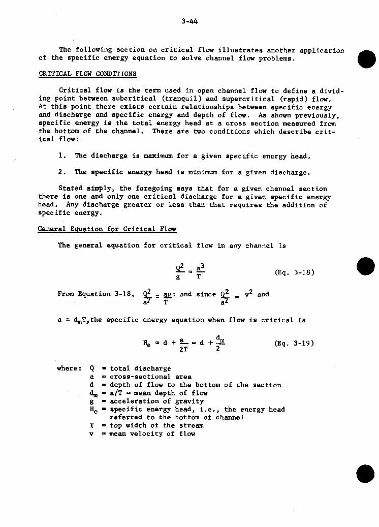
The general equation for crit ical flow i n any channel is

(Eq. 3-18)

From Equation 3-18, * = a~,:and s ince $ v2 and % T

a = d,,,T,the s p e c i f i c energy equation when flow i a c r i t i c a l is

(Eq. 3-19)

where: Q = t o t a l discharge a - cross-sec t iona l area d - depth of flow t o the bottom of the sec t ion d,= a / T - mean'depth of flow g - acce le ra t ion of grav i ty % - s p e c i f i c energy head, i.e., the energy head

r e fe r r ed t o the bottom of channel T = top width of the stream v - mean v e l o c i t y of flow

a

3-45

B A study of the specific energy diagram, Figure 3-12, w i l l give a more

thorough understanding of the relationship6 between discharge, energy, and depth when flow is c r i t i c a l .

Figure 3-12 The Speci f ic Cnergy Diagram

While studying th i s diagrm, consider the follmlng c r i t i c a l flow terms and the i r def ini t ions:

Cr i t ica l Dischaxne The maximum discharge for a given specific energy, or a diecharge

which occurs with minimum specific energy.

Cr i t ica l DepthThe depth of flaw at which the dlecharge is meximwn for a given

specific energy, or the depth a t which a given diecharge occur8 with minimum epecific energy.

Critica1 Velocity The mean velocity when the discharge f6 c r i t i c a l .

Critical SlopeThat d o p e which will sustain a given diecharge a t uniform, c r i t i c a l

depth i n a given channel.

Subcritical Flm Those conditions of flcw for which the depth i 6 greater than c r i t i c a l

and the velocity is lees than c r i t i c a l .

Supercritical Flm Thoae conditions of flow for which the depth is leas than crit ical-

and the velocity is greater than c r i t i c a l .

3-46

The curve shave t h e v a r i a t i o n of s p e c i f i c energy with depth of flaw for a constant Q i n a channel of a given croas sec t ion . Similar curves for any discharge at a s e c t i o n of any form may be obtained from Equation 3-17. Cer ta in poin ts , as i l l u s t r a t e d by t h i s curve, should be noted:

1.

2 .

3.

4.

5 .

I n a epec i f i c energy diagram the pressure head and v e l o c i t y head are shown graphica l ly . The pressure head, depth i n open channel flow, i e represented by the hor izonta l scale as the d i s t ance from the v e r t i c a l axis t o the line along which H, - d , t o the curve of constant Q.

For any discharge the re i s a minimum s p e c i f i c energy, and the depth of f l o w corresponding to t h i s minimum s p e c i f i c energy i s t h e c r i t i c a l depth. For any s p e c i f i c energy g r e a t e r than t h i s minimum t h e r e are two depths, sometime8 ca l l ed a l t e r n a t e s tages , of equal energy a t which the d i s charge may occur. One of these depths is i n the subc r i t ical range and the o ther ie in t he s u p e r c r i t i c a l range.

At depths of flow near t he cr i t ical f o r any discharge, a minor change i n s p e c i f i c energy w i l l cauee a much g r e a t e r change i n depths.

Through the major po r t ion of t he e u b c r i t i c a l range the v e l o c i t y head f o r any diecharge La r e l a t i v e l y small when compared t o s p e c i f i c energy, and changes i n depth are approximately equal to changes i n s p e c i f i c energy.

Through the s u p e r c r i t i c a l range the v e l o c i t y head for any discharge increases rapidly as depth decreases, and changes i n depth are assoc ia ted with much g r e a t e r changes i n s p e c i f i c energy.

I n s t a b i l i t y of Critical Flow

The i n s t a b i l i t y of uniform flow a t o r near crit ical depth is usual ly defined i n terms of cr i t ica l slope, sc.

sc = c r i t i c a l slope - t h a t slope which w i l l s u s t a i n a given discharge i n a given channel a t uniform, c r i t i c a l depth.

The cr i t ical slope, sc, is:

8, = 14.56 n2h (Eq. 3-20)7 7 3

Uniform flow a t ox near c r i t i c a l depth is unstable. This r e s u l t s from the f a c t t h a t the unique r e l a t ionsh ip between energy head and depth of flow which must exist i n c r i t i c a l flow is r e a d i l y disturbed by minor change6 i n energy. Those who have seen uniform flow at or near c r i t i c a l

- - - - -

3-47

depth have observed the uns tab le wavy sur face t h a t i s caused by apprec i a b l e changes i n depth r e s u l t i n g from minor changes i n energy. This uns tab le range i s defined as follows:

Unstable zone i n the range 0.7sc< s o < 1 . 3 s c

where<= the symbol for "is less than"

Because of t h e uns tab le flow, channels car ry ing uniform flow at or near c r i t i c a l depth should not be used unless the s i t u a t i o n allows no a l t e r n a t i v e . In this case allowance must be made i n design for t he height of the wave generated. Often when topography restricts the channel slope t he flow can be fmced i n t o s u b c r i t i c a l stable or s u p e r c r i t i c a l s t a b l e by varying the width of the channel.

Open Channel Problems

Example 3-19 Given : Trapezoidal sect'ion

n = 0.02 s = 0.006

To determine: Q i n c f s , and v i n fps

Solution: from Exhib i t 3-13

bd + zd2 8(2.5) f 2(2.5 2 = 1.695

= = rE=8 + Z ( 2 . 5 ) /-e n t e r Exhibit 3-14 with r = 1.695, s = 0.006, n = 0.02,

and read v = 8 .19 f p s

then Q = av = 32.5(8.19) = 266 c f s

Example 3-20 Given: Triangular s ec t ion

n = 0.025 s = 0.006

To determine: Q i n c f s and v i n fps

3-48

Solution: from Exhibit 3-13

enter Exhibit 3-14 with r = 1.455, s = 0.006, n =: 0,025 and read v = 5.91 f p s

then Q = av = 36(5.91) = 213 f p s

Example 3-21 Given: Trapezoidal section

Q = 300 cfs n = 0.02 s = 0.0009

To determine: d in ft. and v in ft/sec.

Solution: This can be solved by trial. F i r s t , assume a value for d and compute the values of a, p , r;.then from E x h i b i t 3-14 f i n d v and compute Q.

-Trial d -a E r v_ 9. 1 3.0 63.0 20.42 2.21 3.80 239.4

2 3.5 77.0 30.65 2.51 4.14 318.8

3 3.3 71.3 29.76 2.39 3.98 283.8

Plot d against Q for trial 2 and 3 and read d = 3.39 f t . , for Q = 300 c fs

r

3.5-

1 280- 290 300 310 320

Q

3 -49

B For those having much of t h i s work to do, t h e use of t a b l e s i n

King's Handbook, based on the equat ion K' =i QTJ , w i l l provide rap id d i r e c t so lu t ions , i . e . , b8/3 ,1/2

then K' = (300)(*02)= 0.146 (1370 ) ( .03 )

From the t a b l e of K ' va lues f o r 2:l sides and R1 = 0.146

-D = 0.226 b

D = (15)(0.226) = 3.39 f e e t

The same procedures can be followed i n so lv ing for t r i a n g u l a r sect ions.

7. WEIR FLOW

A weir is a notch of r egu la r form through which water flows. The s t r u c t u r e conta in ing the notch is also c a l l e d a w e i r . The edge over which the water flows i s the crest of t he w e i r . Two types of w e i r crests are common i n s o i l conservat ion work, sharp-crested weirs and broad-crested weirs.D

The sharp-crested w e i r i s used only t o measure the discharge of a channel or stream. The sharp edge causes the water t o sp r ing clear of the crest ,

Most hydraul ic s t r u c t u r e s i n s o i l conservat ion work have broad-crested w e i r s . The crest i s hor i zon ta l and long i n t h e d i r e c t i o n of flow so t h a t t he water l a y s on the crest r a t h e r than spr inging clear. The primary use of the broad-crested w e i r is f o r the con t ro l o f f lood flows, although water measurement can be incorporated as a secondary func t ion . Chapter 6 , S t ruc tu res , of t h i s manual desc r ibes i n d e t a i l i t s many app l i ca t ions .

Examples of t he two types of w e i r crest are shown i n F igure 3-13 and 3 - 1 4 .

Figure 3-13 Sharp-crested weir

3-50

Approachchannel -

Figure 3-14 Broad-crested weir

If the overflowing sheet of water (nappe) discharges into the a ir , as above, the weir has free discharge. If the discharge i s partially under water, as shown in Figure 3-15, the w e i r i s submerged or drowned.

Figure 3-15 Submerged weir

BASIC EQUATION

The basic equation for a l l weirs is:

Q = CLH3/2 (Eq. 3-21)

where :

Q = discharge H = measured head L = length of weir C = weir coeff ic ient

Corrections are required to include e f f ec t s of end contractions, velocity of approach and submergence.

3-51

D CONTRACTIONS

The w e i r i s contracted when the respect ive dis tances from the s ides and the bottom of the channel of approach t o the s ides and c r e s t of the w e i r are grea t enough t o allow the water f r e e lateral approach t o the c r e s t . I f the w e i r conforms t o the s ides of the approach channel above the crest and the channel s ides extend downstream beyond the c r e s t , thereby preventing lateral expansion of the nappe, the w e i r has end contract ions suppressed.

. End contract ions reduce the e f f e c t i v e length of a weir. To allow f o r end contractions, the length of w e i r i n the basic equation i s adjusted as follows :

L = L' - O.1NH (Eq. 3-22)

where :

L = e f f e c t i v e length of w e i r L' = measured length of w e i r N = number of contract ions

The above equation i s generally applied only f o r sharp-crested weirs i n s o i l conservation work. For most broad-crested weirs the end contract i o n s will be e i t h e r f u l l y or p a r t i a l l y suppressed. For drop spillways the basic formula can be used without modifying for contract ion e f f e c t .

D VF,LOCITY OF APPROACH

The ve loc i ty of approach is the average ve loc i ty i n the approach channel. It i s measured a t a dis tance of about 3 H upstream from the weir. The veloc i ty head is added t o the measured head t o determine the discharge. Theref ore :

Q = CL ("+&) (Eq. 3-23)

2 312

WE= COEFFICIENTS

Values of the w e i r c o e f f i c i e n t , C , var ies with the type of c r e s t used. Weir coef f ic ien ts f o r sharp-crested weirs normally used in s o i l Conservation work are given under the following sec t ion on water measurement. The weir coef f ic ien t f o r broad-crested weirs c m o n l y used i n s o i l conservation work is C = 3.1.

SUBMERGED FLOW

When a w e i r is submerged, Figure 3-15, the discharge w i l l be less than f o r the head i n f r e e flow. The reduction i n flow can be expressed i n ternis of the r a t i o of the upstream head, H i , t o the downstre& head, H2.

D

3-52

When the r a t i o of H2/Hi for sharp-cres ted weirs reaches 0.3 t o 0.4, t h e d ischarge may be reduced by 5 t o 10 pe rcen t . For H2/H1 r a t i o s of 0.6 t o 0.7, r educ t ions of 20 t o 40 pe rcen t may be expected.

There is no g r e a t r educ t ion i n d i scha rge for broad-cres ted weirs u n t i l the r a t i o of H;!/H1 reaches 0.67. Then t h e d ischarge reduces r a p i d l y as t h e submergence inc reases . For va lues of H2/H1 from 0.75 t o 0.85, reductions from 10 t o 30 pe rcen t occur .

When apprec iab le submergence is t o be encountered, accu ra t e d ischarge can be computed on ly through t h e use of r e f i n e d procedures .

8 . WATER MEASURING

The purpose of t h i s s e c t i o n is t o o u t l i n e t h e most commonly used water measuring methods. The hydrau l i c p r i n c i p l e and equat ion of flow i s given for most methods. For convenience, t h e s u b j e c t i s d iv ided i n t o open channel flow and p ipe flow.

OPEN CHANNELS

The following methods of measurement apply to flows i n open channels .

Orif ices

An o r i f i c e i s a h o l e of r e g u l a r form through which w a t e r flows.

Figure 3-16 Flnw through an o r i t ’ i c c

Flow through an o r i f i c e is i l l u s t r a t e d i n F igure 3-16. The o r i f i c e shown is sharp-edged; i.e., it has a sharp upstream edge so t h a t t h e w a t e r i n pass ing touches only a l ine. If the o r i f i c e d i scha rges into t h e a i r , i t is s a i d t o have f r e e d ischarge ; and i f it d i scha rges under water, i t i s s a i d t o be submerged. O r i f i c e s may be c i r c u l a r , square , r e c t a n g u l a r , or of m y o t h e r regular form.

3 - 5 3

T h e B e r n o u l l i e q u a t i o n w r i t t e n f r o m p o i n t 1 to p o i n t 2, F i g u r e 3 - 1 6 , is

a n d

" P o i n t 2, l o c a t e d w h e r e t h e j e t h a s c e a s e d to c o n t r a c t is k n o w n as t h e v e n a c o n t r a c t a . I t s p r e s s u r e is t h a t of t h e s u r r o u n d i n g f l u i d . F o r d i s - c h a r g e i n t o t h e a t m o s p h e r e P2 is t h e r e f o r e z e r o on t h e g a g e s c a l e . F o r l a r g e t a n k s , vl is so s m a l l t h a t it m a y be n e g l e c t e d . R e p l a c i n g P i / w w i t h h a n d d r o p p i n g t h e s u b s c r i p t of v 2 , t h e e q u a t i o n m a y n o w be w r i t t e n

v = & A h - h A )

N e g l e c t i n g e n e r g y l o s s e s , t h e v t , b e c o m e s

vt = G

e q u a t i o n f o r t h e t h e o r e t i c a l v e l o c i t y ,

T h e e n e r g y l o s s m a y be t a k e n c a r e of by a p p l y i n g a c o e f f i c i e n t of v e l o c i t y Cv to t h e t h e o r e t i c a l v e l o c i t y as f o l l o w s :

v = cv 4 2 g h

T h e d i s c h a r g e t h r o u g h an o r i f i c e is o b t a i n e d v e l o c i t y a n d t h e a r e a at t h e v e n a c o n t r a c t a . T h e t r a c t a , a 7 , is l e s s t h a n t h e a r e a of t h e o r i f i c e ,

( E q . 3 - 2 4 )

f r o m t h e p r o d u c t of t h e a r e a at t h e v e n a c o n - a. T h e r a t i o b e t w e e n

t h e t w o a G e a s is c a l l e d t h e c o e f f i c i e n t of c o n t r a c t i o n C c , T h e r e f o r e ,

a2 = Cca

a n d

Q Z a 2 v 2 = C c a C v x&

T h e p r o d u c t of Cc a n d Cv is c a l l e d t h e c o e f f i c i e n t of d i s c h a r g e C. E q u a t i o n f o r d i s c h a r g e m a y t h e r e f o r e be w r i t t e n

Q = Ca G ( E q . 3 - 2 5 )

3-54

The submerged o r i f i c e in Figure 3-17 is the type most o f t e n used in soil conservation w o r k .

Figure 3-17 Submerged o r i f i c e

As in the free discharge o r i f i c e , Equations 3-24 and 3-25 also a p p l y to the submerged o r i f i c e .

The c o e f f i c i e n t of discharge for submerged o r i f i c e s is approximately the same as that for free discharge orifices. The wide r a n g e in t y p e s of o r i f i c e s and gates, a s p e c i a l form of o r i f i c e , m a k e s it i m p r a c t i c a l to i n c l u d e tables of coefficients c o v e r i n g an a d e q u a t e r a n g e of c o n d i t i o n s . Manufacturers' publications are n o r m a l l y the best source of r e l i a b l e coefficients for v a r i o u s t y p e s o r i f i c e f l o w .

of g a t e s and o t h e r appurtenances involving

W e i r s

Sharp-crested w e i r s are used e x t e n s i v e l y for measuring the flow of water, T'he m o s t common types--rectangular, C i p o l l e t t i , and 90" V - n o t c h weirs--are s h o w n in Figure 3 - 1 8 .

S i d e s s l o p e I horizontal t o 4 v e r t i c a l

R e c t a n g u l a r W e i r Cipolletti W e i r

9 0 ° N o t c h W e i r

Figure 3-18 T y p e s of w e i r s

As g i v e n in the preceding s e c t i o n , Weir F l o w , the b a s i c e q u a t i o n is

Q= CLJIY2

0

, ’ e

3-55

Measurements made by means of a weir are accurate only when the weir is properly set and the head read at a point some distance above the crest so that the reading will not be affected by the downward curve of the water. See Figure 3-19. The weir should be at right angles to the stream at a point where the channel is straight, free from eddies and of sufficient width to produce full end contractions. The crest of the weir must be exactly level for the rectangular and Cipolletti types_ The bottom of the notch must be set above the bottom of the channel a height equal to at least twice the maximum head, preferably more. If a weir is to -continue to give reliable results, it must be maintained ip such a way as to preserve the above-mentioned conditions.

Point to Measure Depth (HI

Sharp- Crested Weir

Figure 3-19 Profile of a sharp-crested weir

3-56

Rectangular Contracted Weir A rectangular contracted weir has its crest and sides so far removed,

respectively, from the bottom and sides of the weir box or channel in which it is set, that full contraction, or reduced area of flow, is developed. See Figure 3-20.

,Point to Measure Depth (HI

Figure 3-20 Rectangular contracted weir

For the rectangular weir the coefficient, C, is 3.33. Allowing for the contractions

Q = 3 33 H3'2 (L-O 2H) . .

where:

Q =

L = H =

discharge in cubic feet per second neglecting velocity of approach the length of weir, in feet head on the weir in feet measured at a point no less than 4 H upstream from the weir.

Discharges may be taken from Exhibit 3-15.

Rectangular Suppressed Weir A rectangular suppressed weir has its crest so far removed from the

bottom of the approach channel that full crest contraction is developed. The sides of the weir coincide with the sides of the approach channel which extend downstream beyond the crest and prevent lateral expansion of the nappe. A suppressed weir in a flume drop is illustrated in Figure 3-21.

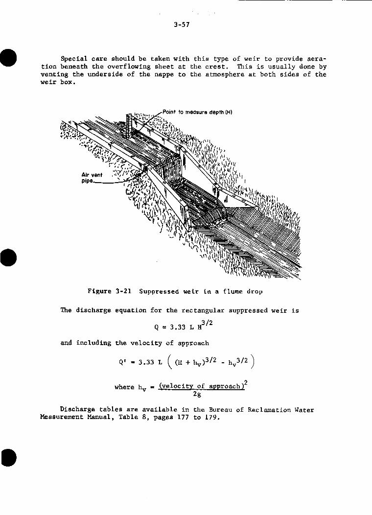
3-57

Special care should be taken with this type of weir to provide aera- tion beneath the overflowing sheet at the crest. This is usually done by venting the underside of the nappe to the atmosphere at both sides of the weir box.

Figure 3-21 Suppressed weir in a flume drop

The discharge equation for the rectangular suppressed weir is

Q = 3 33 I 1-13'2 l

and including the velocity of approach

Q' = 3.33 I (H + hv)31* - hv3i2

where hv = (velocity of approach) 2

2g

Discharge tables are available in the Bureau of Reclamation Water Measurement Manual, Table 8, pages 177 to 179.

3-58

Cipolletti Weir A Cipolletti weir, Figure 3-22, is trapezoidal in shape. Its crest

and sides, which are of thin plate, are so far removed from the bottom and sides of the approach channel as to develop full contraction of flow at the nappe. The sides incline outwardly at a slope of 1 to 4.

Since the Cipolletti weir is a contracted weir, it should be installed accordingly. Jlowever, its discharge is essentially as though its end contractions were suppressed. The effect of end contractions in reducing discharge has been overcome by sloping the sides of the weir.

Figure 3-22 Cipoll.etti =ir

The equation generally accepted for computing the discharge through Cipolletti weirs with complete contractions is:

Q = 3.367 I H312

The selected length of notch (L) should be at least 3H and preferably 4H or longer.

Discharges may be taken from Exhibit 3-16.

3 - 5 9

90' V - N o t c h Weir The c r e s t o f the 90° V - n o t c h weir c o n s i s t s o f a thin p l a t e , the s i d e s

o f the n o t c h b e i n g i n c l i n e d 45' from the vertical. This whir has a con- t r a c t e d n o t c h and all conditions for a c c u r a c y s t a t e d for the s t a n d a r d con- t r a c t e d rectangular weir a p p l y . The m i n i m u m d i s t a n c e from the side o f the weir t o the c h a n n e l bank s h o u l d b e m e a s u r e d h o r i z o n t a l l y from the p o i n t w h e r e the m a x i m u m w a t e r s u r f a c e intersects the edge o f the w e i r . The minimum b o t t o m d i s t a n c e s h o u l d b e m e a s u r e d b e t w e e n the p o i n t o f the n o t c h and the c h a n n e l f l o o r -

F i g u r e 3-23 90° V - n o t c h weir

The V - n o t c h w e i r , F i g u r e 3 - 2 3 , i s especially u s e f u l for measuring s m a l l discharges. The discharge equatioti used i s

Q = 2 5 2 H 2 * 4 7 .

w h e r e

H = v e r t i c a l d i s t a n c e i n feet b e t w e e n the elevation o f the v o r t e x o r l o w e s t part o f the n o t c h and the elevation o f the weir p o n d .

E x h i b i t 3-17 may b e used for determining the discharge.

3-60

Parshall Flume

With a Parshall flume, Figure 3-24, the discharge is obtained by measuring the loss in head caused by forcing a stream of water through the throat section of the flume, which has a depressed bottom.

Plan

ter surface s -- - __ --- z-z_= - . . . . . . . . _ _ _ . . - - - . . - -.

-------

k’igure 3-24 Parshall flume

3-61

There is no need of a pond above the Parshall flume as the velocity of approach has little effect on the'accuracy of the measurement. It uses a small amount of head and can have a high degree of submergence without having to make corrections in the free-flow formula. It does not clog readily with floating trash and keeps itself clean of sand and silt. It requires but one reading of head (Ha) for determining the discharge except in cases of extreme submergence when both Ha and Hb should be read.

Table 9-14, Chapter 9, Section 15, of the National Engineering Manual gives free-flow discharge values .for the Parshall flume.

Trapezoidal Fluine

The trapezoidal flume, Figure 3-25, obtains the discharge by measuring the loss in head caused by forcing a stream of water through the throat of a flume with a level bottom. See Figure 3-25.

An advantage of the trapezoidal flume is that the cross, section corre- sponds to the shape of the common irrigation channel, It is particularly suited for use in concrete lined irrigation channels.

The equation for discharge derived by Robinson and Chamberlain (Transactions of the ASAE, 1960) is

(Eq. 3-29)

where:

discharge, cfs area at the flume entrance, sq.ft. head at the entrance, ft. head at the throat, ft. discharge coefficient that includes the geometry of the structure

Further information on the trapezoidal flume can be found in USDA Agricultural Research Service Bulletin 41-140, dated March 1968.

Current Meter

Basically, the current meter is a wheel having several cups or vanes, This wheel is rotated by the action of the current and the speed of the rotating wheel indicates the velocity of the current, based on a rating table furnished by the manufacturer.

A zero station or reference point is established on one bank of the strem, and a tape is stretched across the stream for measuring horizontal distances. Soundings and current-meter readings are taken at verticals spaced at regular intervals, usually from 2 to 10 feet, depending on the width of the stream, Readings also should be made where there are abrupt changes in velocity or in the depth of flow,

3-62

Plan Vi0w

Profile Vi8w

End View

@I Throat Section

Figure 3-25 Trapezoidal flume

3 - 6 3

A connnon method u s e d to determine m e a n v e l o c i t y r e q u i r e s t h a t read- i n g s be taken at o n l y t w o points in e a c h vertical; namely, 0 . 2 a n d 0 . 8 of t h e sounded depth m e a s u r e d f r o m t h e water s u r f a c e . T h e average of these t w o r e a d i n g s is t h e m e a n v e l o c i t y in t h e vertical. Where t h e depth is t o o shallow t , o obtain t w o readings, o n e reading taken at 0 . 6 depth w i l l repre- s e n t t h e m e a n velocity.

T h e discharge of e a c h segment of stream between a d j a c e n t verticals is t h e product of t h e a r e a o$ t h e segment a n d t h e m e a n v e l o c i t y in t h e s e g m e n t . If d1 a n d d2 represent t h e depths of f l o w at t w o a d j a c e n t verticals, V I a n d v2 t h e r e s p e c t i v e m e a n v e l o c i t i e s in these v e r t i c a l s , a n d W t h e d i s t a n c e between t h e v e r t i c a l s , t h e n t h e discharge in t h a t p a r t of t h e cross section is c o m p u t e d as f o l l o w s :

Q = W c d 1 ; '2xv1 ; v 2 )

T h e total discharge of t h e stream is t h e s u m of s u c h computations f o r t h e entira cross s e c t i o n .

S e e Reference ( 1 ) f o r m o r e d e t a i l e d information.

Water-Stage R e c o r d e r

A water-stage r e c o r d e r c o m b i n e s a clock a n d an i n s t r u m e n t t h a t draws a graph representing t h e r i s e a n d f a l l of a water surface w i t h respect to time. Water-stage recorders a r e in c - o n u s e at permanent gaging stations.

Water-stage recorders a r e desirable under t h e following conditions:

1. T h e f l o w in t h e stream or channel f l u c t u a t e s r a p i d l y , a n d o c c a s i o n a l s t a f f - g a g e r e a d i n g s would n o t g i v e a satisfactory e s t i m a t e of d i s c h a r g e .

2. T h e gaging station is h a r d to g e t t o , or t h e available observers a r e n o t reliable.

3. There is a n e e d f o r c o n t i n u o u s records of f l o w f o r legal or technical purposes.

By t h e c o m b i n e d u s e of t h e s t a g e - d i s c h a r g e curve (Figure 3-26) a n d t h e water-stage recorder, a h y d r o g r a p h of t h e f l o w in a stream or channel m a y be 'plotted. A h y d r o g r a p h is a curve developed by p l o t t i n g discharge on a v e r t i c a l scale against t i m e plotted on a h o r i z o n t a l scale, I h e a r e a beneath t h e curve r e p r e s e n t s t h e volume of water passing t h e gaging station during a n y s e l e c t e d t i m e period.

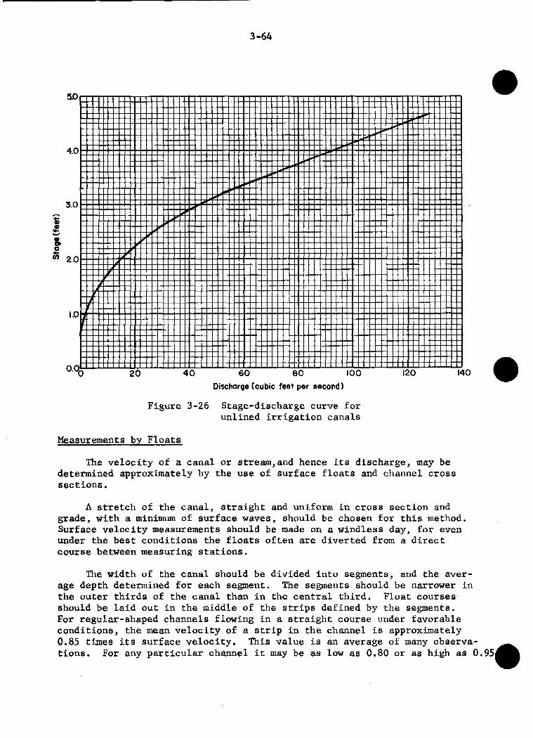
3-64

o.o~‘l”“““‘L”““““‘l”““““““““““ll””””””””~~~’.’ 20 40 60 60 IO0 I20 I40

D i s c h a r g e (cubic f e e t per s e c o n d )

Figure 3-26 Stage-discharge curve for unlined irrigation canals

Measurements by Floats

The velocity of a canal or stream,and hence its discharge, may be determined approximately by the use of surface floats and channel cross sections.

A stretch of the canal, straight and uniform in cross section and grade, with a minimum of surface waves, should be chosen for this method, Surface velocity measurements should be made on a windless day, for even under the best conditions the floats often are diverted from a direct course between measuring stations.

The width of the canal should be divided into segments, and the average depth determined for each segment. The segments should be narrower in the outer thirds of the canal than in the central third. Float courses' should be laid out in the middle of the strips defined by the segments. For regular-shaped channels flowing in a straight course under favorable conditions, the mean velocity of a strip in the channel is approximately 0.85 times its surface velocity. This value is an average of many observa- tions. For any particular channel it may be as low as 0.80 or as high as 0.95

3-65'

The velocity of the float in each str+p, after being adjusted to mean velocity, multiplied by the cross-sectional area of the strip, will give the discharge. The sum of the discharges of the strips is the total discharge. On small streams, rather than dividing the stream into segments a number of float runs can be made and an average of these used for surface velocity of the stream. The float method is an approximate and should be used only with its limitations in mind.

Slope-Area Method

The slope-area method consists of using the slope of the water in a uniform reach of channel, and the average cross-sectional area

the method

surface of that

reach, to give a rate of discharge. The discharge may be computed from Manning's Equation 3-16:

Q= _ ar213$3i2 1.486 n

A straight course of the channel should be chosen, at least 200 feet and preferably 1,000 feet in length, The course should be free of rapids, abrupt falls, sudden contractions, or expansions.

The slope of the water surface may be calculated by dividing the difference in the water surface elevations at the two ends of the course by the length of the course. If it is desired to develop a stage-discharge curve for the channel, gage points, carefully referenced to a common datum level, should be placed one on each bank of the channel and one in the center of the stream, in stilling-wells if possible;

In irregular channels, the area and the wetted perimeter at several cross sections is required and a mean value should be used in computing hydraulic radius.

Inasmuch as the proper selection of the roughness factor n for many streams is difficult, the discharge determined by the slope-area method is only approximate. Care must be taken to determine the slope and areas simultaneously when the water levels are changing. Various hydraulic text- books and handbooks provide tables to assist in the computation of discharges from the above field data.

Velocity-Head Rod

The velocity-head rod is a simple inexpensive rod that can be used to measure the approximate velocity in open channels, if depths and velocities are not too great. This infrequently'-used method is discussed in detail in Chapter 9, Section 15, SCS National Engineering tindbook.

3-66

PIPE FLOW

The following m e t h o d s may be used in d e t e r m i n i n g pipe flow:

O r i f i c e Flow

Pipe orifices, Figure 3-27, u s u a l l y are c i r c u l a r o r i f i c e s placed in or at the end of a horizontal pipe. The head on the o r i f i c e is m e a s u r e d with a manometer_

Where the o r i f i c e is placed in the pipe, the discharge will not be free and the head must be m e a s u r e d at points both u p s t r e a m and downstream from the o r i f i c e . For a f u r t h e r discussion of this type of o r i f i c e , refer to King's h a n d b o o k of H y d r a u l i c s ,

The pipe o r i f i c e c o m m o n l y used in measuring irrigation water and the discharge from wells within a range of 50 to 2,000 g a l l o n s per minute has the c i r c u l a r o r i f i c e l o c a t e d at the end of the pipe_

The pipe must be level. A glass-tube manometer is placed about 24 inches u p s t r e a m from should be closer than 4 the o r i f i c e d i a m e t e r to g r e a t e r than 0,83. The to flow full. The head c a r p e n t e r ' s rule.

the o r i f i c e . No e l b o w s , valves,-or other f i t t i n g s feet u p s t r e a m from the manometer. The ratio of the pipe d i a m e t e r should be no less than 0.50 nor ratio to be selected, h o w e v e r , must cause the pipe in the manometer is m e a s u r e d with an o r d i n a r y

MUST BE LEVEL

A pipe cap this way moy be used as the orifice plate-

Figure 3-27 Pipe o r i f i c e

3-67

D i s c h a r g e t h r o u g h t h e o r i f i c e is c o m p u t e d by E q u a t i o n 3-25, or it can be read d i r e c t l y from E x h i b i t 3-18.

where:

Q- C l =

o r i f i c e d i s c h a r g e in g a l l o n s p e r minute c o e f f i c i e n t which varies with t h e ratio of t h e o r i f i c e

a= g-

d i a m e t e r to t H e pipe d i a m e t e r as well as with a l l t h e other f a c t o r s a f f e c t i n g flow in o r i f i c e s . T h e value of t h e c o e f f i c i e n t (C)may be t & n fran Figure 3-28 c r o s s - s e c t i o n a l area of t h e o r i f i c e in square inches a c c e l e r a t i o n d u e to g r a v i t y - 32.2 feet p e r second p e r second

h= head on t h e o r i f i c e in Inches m e a s u r e d above i t s center

Q - CaJ2gh

Figure 3-28 O r i f i c e c o e f f i c i e n t s

3-68

California Pine Method

B, R. Vanleer developed a method for measuring the discharge from the open end of a partially-filled horizontal pipe discharging freely into the air. 'Ihis method can also be adapted to the measurement of discharge in small open channels where such flow can be diverted through a horizontal pipe flowing partially full and discharging freely into the air.

The method has four requirements for accurate results: 1) The discharge pipe must be level; 2) it must discharge partially full; 3) it must discharge freely into air; and 4) the velocity of approach must be a minimum. Figure 3-29 illustrates one method of meeting these requirements. Other designs may be possible. With such an arrangement, the only measurements necessary are the inside diameter of the pipe and the vertical dis- tanoe from the upper inside surface of the pipe to the surface of the flowing water at the outlet end of the pipe. me discharge may then be computed by the equation:

Q= (Eq. 3-30)

where Q - discharge in cubic feet per second a = distance, in feet, snzasured at the end of the pipe,

frcm the top of the inside surface of the pipe to the water surface

d - internal dieter of the pipe in feet.

This equat.ion was developed from experimental data for pipes 3 to 10 inches in diaeter. In tests made by the Soil Conservation Service it was discovered that for depths greater than one-half the diameter of the pipe, or a/d less than 0.5, the discharges did not follow the equation. Extreme care should therefore be taken in using the equation and tables for conditions where a/d is less than 0.5.

Flow

Figure 3-29 Measuring flow by the California pipe method

0 -

3-69

Tables 48 and 49 in the Water Measurement Manual, Bureau of Eeclama- tion, provide assistance for solvingethe equation for discharge.

Coordinate Method

In this method, coord%natea of the jet issuing from the end of a pipe are measured. The flw from pipes may be measured whether the pipe ia discharging vertically upward, horizontally, or at sane angle with the horizontal. Since the discharge pipe can be set in a horizontal position for measurement purpot3e8, there is no need here for a discussion of flw from pipe in an angular position.

Coordinate method6 are used to measure the flw from flwing wells (discharging vertically) and from small pqing plants (discharging hori- gontally). These methods have limited accuracy wing to the difficulty in making accurate measurements of the coordinates of tha jet. They should be used only where facilities for making more accurate maeurementa by other methoda are not available and where an error of up to 10 percent is permia- Bible.

Figure 3-30 Bequired meaeurementa to obtain flw from vertical pipes

To measure the flw frw pipes diecharging vertically upward, it is necessary to measure only the inside diameter of the pipe and the height of the jet above the pipe outlet (H), Figure 3-30. Exhibit 3-19 gives discharge values for pipe diameters up to 12 inches and jet heights up to 40 inches,

3-70

To measure the flow fran pipes discharging horizontally, it is neceB- eary to'meaeure both a horizontal ar~I a vertical distance from the top of the ineide of the pipe to a point on the top of the jet. gee Figure 3-31. These horizontal and vertical distances ere called X and Y ordinates, respectively.

Figure 3-31 Required measurements to obtain flow fra horizontal pipes

For reasonably accurate reeulte, the discharge pipe must be level and long enough to permit the water to fluw smoothly ae it iaeuets from the pipe. 0 Exhibit 3-20 gives dimcharge valuee for pipe diameters up to 6 inches where the ordinate X ie eelected to be 0, 6, 12, or 18 inches. For pipes flowing leee than 0.8 full at the end, the vertical distance Y can be measured at the end of the pipe where X - 0. Exhibit 3-20 is used to obtain the dia- charge. Exhibit 3-20 ia also applicable either to conditions of full flm or partial flow.

3-71

1 mill ion gallon (mg)

1 cubic foot

1 acre foot (amount of water required t o CoYer one ecre one foot drop)

m1s T I N S THIS CfVeS YOU THIS I I

.1337 cubic f a s t ( C U f t )

3,0689 ec re f e e t ( ac re - f t )

1,728 cubic inchor

7 . 4 0 gal lonr

43.560 cubic f e e t

325,850 ga 1 Ion8

c I 231 cubic inchem (cu in.) I

12 m

acra Inch..

MIGHT

1 ga l lon

1 cublc f o o t

8 . 3 3 wundr ( lb)

62.4 p o d 4

1 g r l l o n par ainucr ( g p )

1 million ~ a l l ~ n par 24 hour. (wd)

I 1 cubic foot por rocond

0.00223 cubic foot per roeond ( c f s )

1,440 g.llon* plr day (24 houri)

1.M7 cubic f e e t psr second

69 5 gallon. psr minute

7.48

448.8

66b,272

.992

gallon. per recond (gps)

ga l lon r p.r minuta

ga1lonr pmr day ( 2 4 hours)

A C ~ O inch p r hour

- 1/ - 2/ I n Arizona, C a l i f o r n i a , Montana, Nevada 4nd Oregon In Idaho, Kaneae, Nebrarke, New ~ x l c o , North Dakotr. South Dakota, and Utah

1.983

GO

so

38.4 T

Exhibit 3-1 Water volume, weight and F l o w equivalents

acro foot per day (2b houri)

minor ‘ I incher ( l e g a l value 2’)

m i n e r ‘I inchar (lmgal v a l w ?I)

miner ‘I incher ( i n Colorado)

1 m i n e r ’ u inch

35 .7 miner‘s inchem ( i n B r i t i s h Columbia)

11.25 gpm when equivalent t o 1/40 recond foot

9 gpa h e n equivalent t o 1/50 occond foot

3-72

Exhibit 3-2 Preraure diagrms and methods of computing hydrostatic loads (Ref. NEH Section 5 , ES-31)

(Sheet 1 of 2 )

3-73

Exhibit 3-2 Pressure diagrams and methods o f cmputinn hydrostatic loads (Ref. NEH Section 5 , E S - 3 1 )

(Sheet 2 of 2 )

3-74

$--J . . . .

. . . . . .

. . . .

. . . . . . . -

. . . . . . . . . . . .

. - . . j 1

2ao

2 0.0

15.0

iao

w ao 9.0

F

T.0

a*o

W 1.0 x 3

4.0

10

L.0

I.

I .o 1 .1 2.0 5.0 4 a SO 6.6 7.0 110 90 K,

THICKNESS OF BOARD IN INCHES

. . . . . . . .

. . . . . . , . . . . . . . . . . . . . . ........ "/,,1 ;, ,:.-.-..j.;.i.; . , . . . . . . . . . , , , , , , .

. , . . , . . ,

I .o 1.5 2.0 CORRECTION FACTOR

Exhibit 3-3 Required thickness of flashboards ( re f . Western Stares Engineering Handbook Section 6)

3-75

Exhibit 3-4 Head loss coefficients for circular and square conduits floving full ( R e f . NEH Section 5 , E S - 4 2 )

3-76

h

Exhibit 3-5

Discharge of circular pipes flowing

full.

:4anning'tr n

5 G.010

(Sh

eet 1 of 6)

Exhibit 3-5

Discharge of-circular pip

es

flow

ing

full.

Manning’s n

= 0.011

(Ref. N

ElI C

ec

tion

5, es-54>

(S

heet 2

of 6)

3-78 A!! *

Exhibit 3-5

Disch

arge of circula

r pip

es flowing fu

ll. (Sheet 3 of 6

) 'dlanning's

n - 0.012

3-79

Exhibit 3-5 D

ischarge of circular p

ipes flowing fu

ll. llanning's

(Sheet 4 Of 6

) n = 0.013

(Hef.

NEII Section 5, E

S-54)

Ex

hib

it 3-5 D

ischarge o

f circu

lar p

ipes flowing

full.

'Ianning's n

= 0

.01

4

(Sheet 5 of 6)

Exhibit 3-5

Disch

arge oi circciill- p

ipcs

flowing full.

t.!an

nin

g's

n

= <).u24 (S

heet 6 of 6

)

3 -84

1%-inch 1%-inch 2-inch

1.502 I D 1.720 I D 2.149 I D

Q Gallons per min

2%-inch 3-inch 3t-inch

2.601 I D 3.166 I D 3.620 I D

2 4 6 8

10

15 20 25 30 35 40 45 50

55 60 65 70 75 80 85 90 95

100

110 120 130 140 150 160 170 180 190 200

220 240 260 280 300 320 340 360 380 400

420 440 460 480 500

1-inch

1.189 I D

.15

.54 1.15 1.97 2.98

6.32 10.79 16.30 22.86

F r i c t i

.04

. 1 7

.37

.63

.95

2.03 3.46 5.22 7.32 9.75

12.46 15.51 18.87

22.48

I Head Lo

.02

.09

.19

.32

.49

1.04 1.78 . 2.70 3.78 5.03 6.46 8.02 9.75

11.64 13.64 15.85 18.19 20.65 23.28

Table based on Hazen-Williams equation - C1 = 150

i n Feet e r Hundr -7- .03 .06 . l l .16

.35

.60

.91 1.27 1.70 2.18 2.71 3.30

3.94 4.62 5.36 6.14 6.99 7.86 8.81 9.79

10.82 11.89

14.21 16.69 19.35 22.21

To find f r i c t i o n head loss in PVC or ABS pipe having a standard dimension r a t i o other than 21, t he values i n the t ab le should be mul t ip l ied by the ap- propr ia te conversion f ac to r shown below:

SDR No. 13.5

Conversion Factor

1.35 1 7 1.13 21 1.00 26 .91 32.5 .04 41 .785 51 .75

. 01

.02

.04

.06

.14

.23

.36

.50

.67

.86 1.07 1.30

1.54 1.81 2.10 2.42 2.75 3.10 3.47 3.85 4.25 4.69

5.59 6.56 7.63 8.73 9.94

11.20 12.51 13.90 15.39 16.91

20.19 23.73

Feet

.01

.02

.05

.09

.13

.19

.25

.32

.40

.49

.59

.69 ' .80

.92 1.06 1.19 1.33 1.48 1.64 1 .80

2.14 2.52 2.92 3.36 3.82 4.29 4.80 5.35 5.92 6.50

7 . 7 7 9.12

10.57 12.11 13.78 15.52 17.37 19.27 21.33 23.45

.01

.02

.04

.07

.10

.13

. 1 7

. 2 1

.25

.30

.36

.41

.47

.55

.62

.69

. 7 7

.85

.93

1.11 1.31 1.53 1.75 1.99 2.24 2.50 2.79 3.08 3.38

4.04 4.76 5.51 6.32 7.18 8.10 9.01

10.08 11.13 12.22

13.40 14.59 15.86 17.15 18.50

Q ;allons )er min.

2 4 6 8

10

15 20 25 30 35 40 45 50

55 60 65 70 75 80 85 90 95 100

110 120 130 140 150 160 170 180 190 200

220 240 26 0 280 300 320 340 360 380 400

420 440 460 480 500

Exhibi t 3-7 F r i c t i o n head loss i n semirigid p l a s t i c i r r i g a t i o n p i p e l i n e s manufactured of PVC or ABS compounds. Standard dimension r a t i o - SDR = 21. (Ref. SCS - Fort Worth, Texas, 1967)

S h e e t 1 of 5

3-85

5-inch 6-inch

5,033 ID 5.993 ID

Q Gallons per min.

8-inch 10-inch 12-inch

7.805 ID 9.728 ID 1 1 . ~ 3 8 ID

15 20 25 30 35 40 45 50

55 60 65 70 75 80 85 90 95

100

110 120 130 140 150 160 170 180 190 200

220 240 260 280 300 320 340 360 380 400

420 440 46 0 480 500 550 6 00

4-inch

k.072 I D

* 01 .02 .04 .05 .07 .09 .12 .14

.17

.20

.23 ,27 .31 .35 ,39 .43 .48 .52

. 6 3

.14

.05

.98 1.11 1.26 1.41 1.57 1 .73 1 .90

2.28 2.67 3.10 3.56 4 . 0 4 4.56 5.10 5.67 6.26 6 .90

7.55 8.23

9.67 10.42 12.44 14.61

8.94

.iction L

.01

.02

.02

.03

.04 . 05

.06

.07 ,08 -09 .I1 - 1 2 .14 .15 .17 .19

I22 .26 .30 .35 .40 .44 * 49 .55 .61 .67

.81

.95 1.10 1.26 1.43 1.62 1.82 2.02 2.22 2.45

2.69 2.92 3.18 3.44 3.70 4.42 5.21

Low in

.01 . 01 * 01 .02

.02

.03

.03 -06 .04 .05 .05 .w .07 .07

.09

.10

.12

.14

.16

.19

.21

.24

.26

.29

:M . 40 .46 .54 .61 .69 . 77 .86 .95

1.04

1.14 1.25 1.35 1.46 1.58 1.89 2.22

!et per Hu

. 01

.01 . 01 . 01

. 01

.01

.02

.02

.02

.03

.03

.04

.05

.05

.a -07 .07 . oa

.09 I10 . 12 .14 .17 .19 .21 .24 .26 -28

.31

.34

.37

.41

.43 - 52 .61

red Feet

p R lio. 13.5 17 21 26 32.5 41 51

.01

.01

. 01

.01

.01

.02

.02 * 02 .02

.03

.03

.04

.05

.05

.06 -07 -08 .09 .10

.10

. ll

.12

.14

.15

.18 * 21

b c t o r 1.32 1.13 1.00

.91

.785-

. 75

. a4

. 01 - 01 .01

. 01

.01

.02

.02 ,02 .03 .03 .03 .a5 .04

.05

.05

.06

.06

.w

.07

.09

Q Gallon8 per pin.

15 20 25 30 35 40 45 50

55 60 65 7 0 72 80 85 90 95

100

110 120 130 140 150 160 170 180 190 200

220 240 260 280 3 00 320 340 360 380 400

420 440 460 480 500 550 600

Exhibit 3-7 Frlctlon head loss i n ammirigid plart ie irrigation pipel ine8 manufactured of PVC or ABS compound#. Standard dlmenaion r a t i o - SDR - 21. (Ref. SCS - Fort Worth, Tsxaa, 1967)

Shee t 2 of 5

3-86

Q Gallons per min.

600 650 700 750 800 850 900 950

loo0

1050 1100 1150 1200 1250 1300 1350 1400 1450 1500

1600 1700 1803 1900 2003 2100 2203 2300 2400 2500

2600 2700 2800 2900 3000 3100 3200 3300 3400 3500

3600 3700 3800 3903 4003

4 - i LIC h

4.072 I D

14.61 16.94 19.45 22.08

SOP No. 13.5 17 21 26 32.5 41 51

S-i-cb

5.c33 ID

:iction L

5.21 6 . W 6.92 7.07 8.88 9.93

11.05 12.18 13.40

14.67 16.00 17.39 18.80 20.27 21.78

pact or 1.35 1.13 2 . 0 0

.91

.84

.75

.7a5

1 Loss in

2.22 2.58 2.96 3.36 3.78 4.24 4.71 5.21 5.73

6.27 6.83 7.41 8.02 8.66 9.32 9.99

10.66 11.40 12.13

13.68 15.29 16.99 18.81 20.G6 22.61 24.67

! e t per Hu

.61

.71

.81

.93 1.04 1.17 1.30 1 . M 1.58

1.73 1.88 2.05 2.21 2.39 2.57 2.76 2.95 3.16 3.3s

3.78 4.23 4.70 5 .,20 5.72 6.26 6.83 7.42 8.02 8.67

9.31

10.67 11.39 12.10 12.89 13.66 14.46 15.29 16.11

16.99 17.89

19.69 20.67

9.98

l a . 76

red Feet

.21

.24

.28 - 32

.36

.40 * 44 .49 .54

* 59 .6S .70 .76 * 82 .88 .95

1.01 1.08 1.15

1.30 1.45 1.62 1.79 1.97 2.15 2.34 2.55 2.76 2.97

3.20 3.43 3.67 3.92 4.17 4.43 4.71 4.97 5.27 5.56

5.85 6.17 6.47 6.79 7.11

~

* 09 .10 .12 .14 .16 .17 .19 .21 .23

.26

.28

.30

.33

.35

.37

.40

.43

.47

.50

.56

.62 I 7 0 . 7 7 .84 .93

1.01 1.10 1.19 1.29

1.39 1.49 1.59 1.69 1 .81 1.92 2.01 2.15 2.28 2.41

2.53 2.67 2 .80 2.94 3.03

4 Gal 1 ons per min.

~

600 650 700 150 800

900 950

1000

1050 1100 1150 1200 1250 1300 1350 1400 1450 1500

1600 1700 1800 1900 2000 2100 2200 2300 2400 2500

2600 2700 2800 2900 3000 3100 3200 3300 3400 3500

3600 3700 3800 3900 4000

a50

Bxhlbi t 3-7 PrLction h a d lor8 in m8mirigid plastic irrigation piprlimr unufacturrd of PWZ or ABS compoundm. Stand8rd dlwnrion ratio - SDR = 21. (Rmf. SCS - Fort Worth, Taxaa, 1967)

3-87

4-ipch 6 - i ~ ~ h 8-inccb lO-iacb l l - i ~ ~ h

3.736 ID 5.556 ID 7.382 ID 9.228 ID 11.074 ID

l c t i o a Led Xarm i n Feet Par &adred Pact

Q :allone per d n .

P GAlloar poo min.

15 20 25 30 35 40 45 so 55 60 65 70 75 a0 85 90 95

1 m

110 120 130 140 150 160 170 180 190 200

220 240 260

300 320 340 360 380 400

420 440 460 480 500 550 600

280

.02

.oQ

.w

.09

.12

.15

.18

.22

-27 .31 .36 .42 .47 .53 .60 .66 .73 .80

.96 1.13 1.31 1.50 1.70 1.92 2.15 2.39 2.64 2.90

3.46 4.07 4.72 5.41 6.15 6.93 7.76

9.53 10.48

11.47 12.50 13.58 14.69 15.84 18.90 22.21

8.62

Table baaed on B u e a - V i l l l ~ equation - C1 150.

. 01 . 01

.02

.03

.03

.w

.05

. 05 *a .07 .08 .09 . lo .ll * 11

.14 -16 19

.21

.25

.31

.35

.38

.42

.so

.59

.68

.78

.89 1.00 1.12 1.25

1.52

1*66 1.81 1.96 2.13 2.29 2.74 3.21

.2a

1.38

fa find friction h e 4 lor. In €W or N M pipe having atandard dirsPrloa r a t i o other than 21, the valuer In the table i b u l d be rul - t ip l ied by the appropriate cower- aim fuctor m h o l m be lw:

. 01

. 01

.02 . 01

.02

.02

.03

.03

.03 .w

. 05 * 05 .06 .Of .08 .09 .10 .ll

.13

.15

.17

.20 * 22 .25 .28 .31 .35 .38

.42

.45

.49

.53

.57

.69

.81

13.5 17 21 26 32.5 41 51

* 01 .02 .02 .02 -02 .03 .03 .03 .M

.M

. 05 '.ix .07 .08 .08 .09 . l l .12 I 13

-14 .15 .17 .18 .19 .23 .27

1.34 1.13 1.00

.91

.84

.785

.75

* 01

.02 * 02 .02 .03 .03 .03 .os .oc .05 .05

.a

.a

.07

.07 -0.9 .10 .ll

Exhibit 3-? Friction haad lor8 in remirigid pla8tic irrigation plpllimr manufactured of PVC or ABS coapoundr. Standard d b a a i o n ratio - 5061 - 21. (Uf. SCS - Fort Worth, Taxm, 1967)

15 20 25 30 35 40 45 so

55 60 65 70 75 80

90 95

100

110 120 130 140 150 160 170 180 190 200

220 240 260 280 300 320 340 360 380 400

420 440 W O 480 500 550 600

as

S&.t 4 of 5

3 -88

For PIP Pipe

Q ca110n1 per win.

650 7 0 0 750 800 850 900

LOOO

1050 1100 1150 l2OO 1250 1300 1350 1400 1450 1500

1600 1700 1800 1900 2oqo 2100 2200 2300 2400 2500

26M) 2 700 2800 2900 3000 3100 3200 3300 3400 3500

3600 3700 3800 3900 4000

950

4 - i ~ h

3.736 ID

C-iwcb

5.556 ID

gction Baql

3.73 4.28 4.86 5.47 6.13 6.81 7.53 8.28

9.- 9.87

10.72 11.60 12.51 €3.45 14.43 15.43 16.47 17.54

19.76 22.11 24.58

i&u% 13.5 17 21 26 32.5 41 ' 51

Pacrot 1.34 1.13 1.00

.91

.84

.785

.75

8-ioch

7.382 I D

pmr in F Be

7 93 1.07 1.22 1.37 1.53 1.71 1.89 2.07

1.27 2-47 2.69 2.91 3.13 3.37 3.61 3.87 4.13 4.39

4.95 5.54 6.16 6.81 7.49 8.19 8.93 9.70

10.49 11.32

12.17 13.05 13.96 14.90 15.86 16 * 85 17.88 18.92 20.00 21.10

22.23 23.39 24.57

lO-imh

9.228 I D

per Hundrec

.31

.36

.41

.46

.52

.58

.u

.70

.77

.83

.91

.98 1 . Q 1.14 1.22 1.30 1.39 1.48

1.67 1.87 2.09 2.29 2.52 2.76 3.01 3.27 3.54 3.82

4.10 4 .40 4.71 5.02 5.35 5.68 6.03 6.38 6 .74 7.11

7.50

8.28 8.69 9.11

7.89

12-inch

11.074 I D

feet

.13

.15

.17

.19 * 21 .24 .26 .29

.31

.34

.37

.40

.43 ,47 .50 .54 .57 .61

.69

.77

.85

.94 1.04 1.14 1 .24 1.35 1.46 1.57

1.69 1.81 1.94 2.07 2.20 2.34 2.40 2.62 2.71 2.93

3.08 3.24 3.41 3.58 3.75

Q Gallons per mln.

650 700 750 800 850 900 950

1000

1050 1100 1150 1200 1250 1300 1350 1400 1450 1500

1600 1700 1800 1900 2000 2100 2200 2300 2400 2500

2600 2700 2800 2900 3000 3100 3200 3300 3400 3500

3600 3700 3800 3900 4000

Exhibit 3-7 miction &Fd 1088 in @emirI&id pl8rtlc Irrigation p i p l i - 8 unuf8ctuted of P W or rllBs compoundr. Standard d b n r i o n ratio - 8DR - 21. (Ref. SCS - Fort Worth, Tmxar, 1967)

3-89

PIPE ENTRANCES INWARD PROJECTING PIPE

' HOODED INLET SLIGHTLY ROUNDED

K%

0.70

I .oo K,

0.23

SHARP-CORNERED

RETURN BEND L

STANDARD 90*- ELBOW

K,

2.20

PIPE BENDS

KBO

0.90

BELL MOUTH

STANDARD-TEE

W ..

LONG RADIUS ELBOW

K8

0.50

K,

0.04

KS,

1.80

KLR

0.60

Exhibit 3-8 Head loss coefficients for pipe entrances and bends (Sheet 1 of 2 )

3-90

WIDE OPEN

PIPE BENDS 450 ELBOW

T

K I RPRTIALLY CLOSED

1 ENLARGEMENTS AND CaTRACTIONS

SU-N ENLARGEMENT 1 K,, 1

SUDDEN CONTRMTION

B

GRAWAL ENLARGEMENT

n

K FACTORS FOR A 8rB SEE:

REFERENCE1 HANOBOOK OF HYDRAULICS

BY H.W. KING

PAGES 6 - 18 (FOURTH EDITION)

FOOT VALVE

GLOBE VALVE

0.40

10.00

ANGLE VALVE 15.00

GATE VALVE 10.20 I

FOR K FACTORS SEE: REFERENCE I

BY H. W. KING

PAGES 6 - 18 (FOURTH EDITION)

Exhibit 3-8 Head lor8 coefficient8 for pipe entrances and bends

- 3-91

( 1 ) (2)

- 8.

- 5. - c

--4. - -

- 3.

.------)

I

- e. %: € . a * a - 1.5 w - r 5 - 0

z - =-- t - x p: - 1.0 s - g - .a

W

a W ' I - .a

-.? .

-

- -5

(3) - 6.

- 5. r 6.

- 5.

- 4. - 4.

- - 3. - 3. - - - -

- - * --- - e, .- 2.

* - r *

-1.5 - 1.s - - * - c - - 1.0 - 1.0

- - .B - .B

- - - .8 - .8

- .r - .7

- .6 - .I -

.s - .s

/' /

m W s - c) z E g 3

k

k

c,

E

W = 0 s

LNTRANGE 40 0 TYPE

I06

- S6

- a4

- 7P

- ao

- 5 4

- 4 1 : / 4 0

-36

-33

- 30

- P? - 94

- e l

- 18

- I8

I-

L

10 I

6 I 4 i 3

t 1.0

Exhibit 3-9 Headwater depth for concrete pipe culverts with inlet control (Ref. Hyd. Eng. Cir. No. 5, USBPR, 19 65)

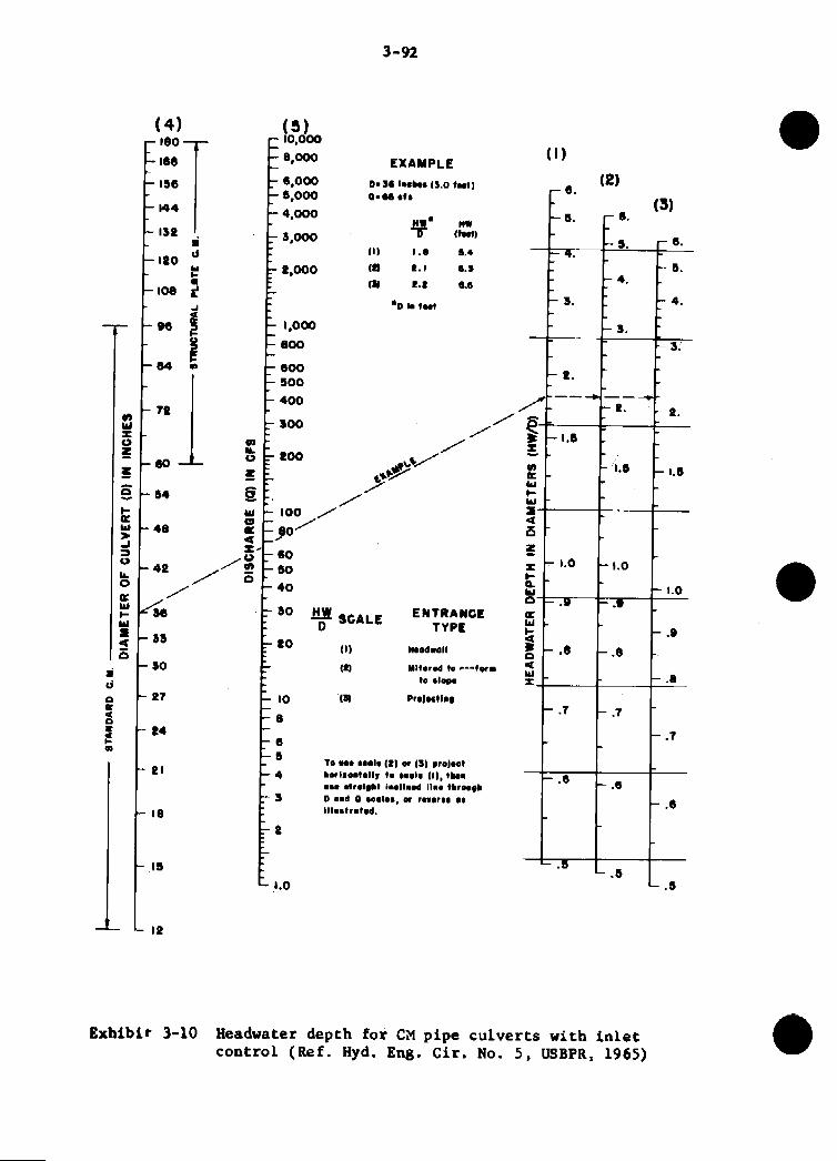
3-92

(4) "T - 144

-60 -.. 1

- 13P -1190

i J

t

-1- d

-me f - 3 -84 5

- 64

- 48

6,000 1:z 5,000

9,000 t 1,000

800

600 so0 400

100

40

t o

10

8

6 8 4

s

9

1.0

t 4

91

i e

IB

IP

LNTRAMGE TYPE

Exhibit 3-10 Headwater depth fox CM pipe culverts with i n l e t control (Ref. Hyd. Eng. Cir. No. 5, USBPR, 1965)

3-93

n - Y - 0 -

z ;

~ 0 0 0 0

-

- 1000

- 800

- 600

- 500

- 400

- 300

*

-

- ; PO0

w e - 4e-:

/* - 4P I

- 36 - 11 - 30

- Pt - 94

- 91

- 18

-18

-11

I L t

f a

I90

I08

91

04

V0

6e 60

rs4 c .

W (D a

e - a I.

Q

TI00

2' r , , y -60

-so

- 40

- SO

- 10

- 10 - 8

- 6

- 9

- 4

-

I

I"

,/- **€pi" <A

0 --

8

10 t 90

Exhibit 3-11 Head for concrete pipe culverts floving f u l l with outlet control n = 0.012 (Ref. Hyd. Eng. Cir. No. 5 , USBPR, 1965)

3-94

m - k - 0 -

t : -?

P 1 u c d 5r

-2000

r 1000 - - 800

- 600

- 500

-- 400

- 300

-

-- eoo

-

100

ZFeo *I

0 : E - r - E

t

g a

- I20

- ioe

- 91

- 84

- 72

- 66

- 60

- 34

- 4 8

42

e-36

,.-33

- 4 7

--- - "48

- e4

- E l

- I 8

- I 5

-19

2 -

!! Q

7.4

-.S

-.6 - -.e - - la

-

F - w - e W IL'

X -

r - 3

- c

Y -

o - 4 -

f w - 4

- 5

- 6

-80

2 - 5 0

O-40 - 0 . 3 1

- 30

- eo

-10 - - a - - 6

- 5

- 4

- 3

-P

Exhibit 3-12 Head for CM pipe culverts flowing full with outlet control No. 5 , USBPR, 1965)

n - 0.024 ( R e f . Hyd. Eng. Cir.

3-95

b k

h

9

k

'b Iy

I N

Exhibit 3-13

Elem

ent8 of channel sections (R

ef. NEH Section 5

, ES-33)

: M.0

am

px)S

M J

lS.0 -5

m w.0

CS.0

m.4

-m.0

IV.0

M.0

0.0 Q-

w.0

IS.0

d t . 0

I I . 0 8 P d

a.0

7.4

cIoDD.Io I.0

S.0 -s

L . 0

t.O

l.0

ao

Exhibit 3-14 Solution o f ?tanning'm formula for uniform flow (Ref. NEH Section 5 , E S - 5 4 )

Sheer 1 o f 4

3-97

t -

11.0

7.0 - -1 4.0 f -3 Dmp

- $

Exhibit 3-14 Solution of thnning'a formula for uniform flow (Ref. NEH Section 5 , ES-54) Sheet 2 of 4

3-98

. ' JJ

J a

:: bnpo d C k r t 5 - a m to a s r - am to 7.0 n - a m t o a070 v - a7 ID 16.0

I J . 0

It.0

,l.Y

m.0

9.0

8.4

7*0

4.0 4 f

9.0 4

4.0

'I -o.o*

3.0

c.0

I. 0

ao

0. t

E x h i b i t 3-14 Solut ion of Manning's formula for uniform flow ( R e f . NEH Section 5 , E S - 5 4 )

3 -99

P U T Of cwrt ~.o.o/o m 0.50 r .O .20 7.0 n . 0 . W M 0.07 Y' 16.0 10 W.0

E -0.0 aw

Exhibit 3-14 Solution of Manning's formula for uniform f l o w ( R e f . NEH Section 5 , ES-54)

S k e t 4 of 4

3-100

- Fed 0. 10 . 11 . 12

. 14

. 1s

. I6

. 17 . 18 . 19

.a0

.21 .n

. 24

. 26

. 27

. .28 . 29

.80

.81

. a2 . 33

. M

. la

. aa

. as

-8s .a6 .87 .a8 .m .40 .41 . 4 2 .48 . 4 4

.4b

. 46

. 4 7

. 4 8

. 4 9

. M )

.61

.52

.5a

.M

.sb

.66

.57

.MI

.59

.Bo '.61 .62 .u .64

I font

3nond-/sc 0. 11 . 12 . 14 . 16 . 17

. 19

. 23

. 25

. 2 7

.29

.a4

.a6

.40

. 4 a

. 4 6

.48 -60

. 68

.65

.5R

, a1

. a1

. a8

. a1 . aa

.MI . m . ?1

. 7 4

.77

.a

.I

.(18

.91

.M

.99 1. M 1. w 1. 08

1. 1 1 1. 15 1. 18 1. 21 1. 25

1. as 1. 81 1. 85 1. 88 1. 42

I. 45 1. 49 1. 52 1. be I. 80

.m

Exhibit 3-15

1.5 feet.

darond-Jrd 0. ItJ . 1R .!lo . 22 .2I

. 2 8

.81

.81

. 8 7 .on

. 42

. 4 7 .w

.M . 17

.8I

. w

.68

.72

.7a

.m

.84 .a

.92

. w 1. 00 1. 01 1. 08

1. 17

1. 21 1. 28 1. XI 1. 86 1. 40

1. u 1. 49 1. 64 1. 19 1. 64

1. ai3 1. 78 1. 78 1. & 1. 88

1. 98 a04 2. 08

2. 20 2 35 2 81 286

1. it

1. m

a 1s

2 4 a

disc ha^, Q, for oreat length, L, of-

2 feet ~

h o d - &

.26

. 28

. 86

. w ; 48 . 4 7 .61 . b s

.sQ .a -6u . ?2 . 77

.a

.86

.91

.MI 1. 03

1. 07 1. 12 1. 18 1. 18 1. I 1. 81 1. ro 1. 41 1. 61 1. 67

1. 8 1. 69 1. 7& 1. 81 1. gs 1. 04 9.00

a. 18 220

+ w

1. 46 1. a 2Bo

2 74 2. 81 9. 88

296

a. 10 8. 17

a d

. az

am

2.88 alro

a 6'1

a m

a m

Discharge for

1 feet

8Wond-jtd 0. 88 . a7

.47

. M

. 4 a

. w

.M

.70

.88

.89

.I 1. M 1. 00 1. 18

1. 28

1. 88 1. 48 1. 58

1. 61 1. 69 1. 77 1. 88 1. p1

1 M 2 11

s.!m

.7a

I. a1

9. Po 2 a7

a 413

a 74

ao8 a 12 a n a a1 x 4 1 8. C1 a 61 s. 78 ass a 09 4. 01 4. 16 4. !M 4. w 4. 47 4. 69 4. 6Q 4. 81

9.16 26s

*a 3.08

4. m

4 feet

Smcomti- mi

.bo

. h7

.64 . 71

. 79

.80 .w 1. 08 1. 11

1. 1Q 1. 28 1. a7 1. 46 1, 56

1. 6s 1. 76 1. 85 1. 9s 2 06

1. 18 2, 26

0. 48 2. 60 2. 71 9. 82

a d

a. a7

294 am a. 18

aso a. 42 a s4 a 67 a 80

a. ea 4. 06 4. 18 4. 82 4. 45

4. I 8 4. 72 4. 88 4. 88 6. 19

6. 49 5. 58 6. 70 5.8s

6. 00 6. 14 6. 29 B. 44 6.58

an

6 feet

Sarond-fttt 0. 62 .7a

. 93 1. 04

1. 15 1. 27 1. 89 1..52 1. 64

1. 78 1. 91 a 06 a. 19 2 BS

2. 48 2. 68 2 78 2. 93

.8a

ao8

a. 2s a 41 8. 58 3. 76 8. 92

4. 08 4. w e 44 4. 62 4. 80

4. w A 17 6. 86 6. 66 8. 76

6. 94 6. 14

6. 64 8.74

7. 15 7. 86 7. 57 7. 79

8.M)

a 34

a 95

a 22 8. 4a a 65 8.88

9. 10 9. 33 8. 66 9. 78 ia o

contracted rectangular

8 feet

* Strond- uut

. 9 7 1. LO 1. 24 1, 39

1. 51 1. 70 1. 86

2. 20

2, 55 2. 78 2. M a. It

0 . J

a. oa

a a7

a 81 a 51 a 71 a a2 4 13

4. 34 4. 66 4. 78 5. 01 6.' 24

6. 47 5. 70 5. 94 6. 18 8. 48

6.67

7. 18 7. 48 7. 68

7. 95 a 22 a 48

6. 9a

a 75 9. oa 9. ao 9. 58 9. $4 10. 1 10. 4

10. 7 11. 0 11. 8 11. 8 11. 9

12.6 12. 8 13. 1

la. 2

la. 4

weirs

10 feet

8econd-ftet 1, 05 1. 21 1. 88 1. 56 1. 74

1. 98 a ia a. a3 2. 58

a 19 a 4a a m a m

2. 7K

2. 97

4. 14 4. 88 4 65 4. 91 5. 17

5. 44 6. 71 6. 99 6. 27 8. 511

6.86 7. 14 7. 44 7. 74

U S 6 8. 87 8.88 9. a1 9. 89

9. OB 10. 8 10. 6 11. 0

11. 7 12. 0 12. 4 12. 7 13. 1

19. 8 14. D 14. 6 14. 9

16. a 15. 7 18. 1 16. 4. 16. 4

a OK

11. a

la. 4

( R e f . Parshall, R.L., Measuring Water in Irrigation Channels, U.S. Dept . Agr. Cir. 843, 1950) (Sheet

3-101

Head, HI

Fed 0. 66 .a . 07 .66 .69

.70 . 71

. 73 . 73 . 74

.76 .76 . 77 .78 .79

.80

.81

. 82

.83

.84

. 85

.86

.87 . 88 - 8 9 .go .91 .92 .93 .94

.95 - 9 6 .97 . 98 . 99

1. 00 1. 01 1. 02 1. 03 1. 04

1. 05 1. 06 1. 07 1. 08 1. 09

1. 10 1. 11 1, 12 1. 13 1. 14

1. 15 1. 16 1. 17 1. 18 1. 19

1 foot

scond-feet 1. 63 1. 67 1. 71 1. 74 1. 78

1. 82 1. 86

1. 92 1. 07

2. 01 2. 05 2. 09 2. 13 2. 17

2. 21 2. 25 2. 29 2. 33 2. 37

2. 41 2. 46 2. 50 2. 54 2. 58 2.' 62 2. 67 2. 71 2. 75 2. 79

2. 84 2. 88 2. 93 2. 97 3. 01

3. 06

1. m

...... __"_.. ....._

Exhib i t 3 -15

1.5 feet

Second-feel 2. 47 2. 53 2. 59 2. I34 2. 70

2. 76 2. 81 2. 87 2. 93 2. 99

3. 05 3. 11 3. 17 8. 23 3. 29

3. 35 3. 41 8. 47 3. 54 3. 60

a. 66 3. 72 3. 79 3. 85 3. 92 3. 98 4. 05 4. 11 4. 18 4. 24

4. 31 4. 37 4. 44 4. 51 4. 57

4. .64 4. 71 4. 78 4. 85 4. 92

4. 9s 5. 05 5. 12 5. 20 5. 26

5. 34 5. 41 5. 48 5. 55 5. 62

5. 09

5. 84 5. 91 5. 98

5.77

Discharge, Q, for crest length, L, of-

2 feet

Second-feel 3. 32 3. 40 3. 47 3. 56 3. 63

3. 71 3. 78 3. 86 3. 94 4. 02

4. 10 4. 18 4. 26 4. 34 4. 42

4. 51 4. 59 4. 67 4. 75 4. 84

4. 92 5. 01 5. 10 5. 18 5. 27 5. 35 5. 44 5. 53 5. 62 5. 71

5. 80 5. 89 5. 98 6. 07 6. 15

6. 25 6. 34 6. 43 6. 52 6. 62

6.71 0. 80 6. 90 6. 99 7. 09

7. 19 7. 28 7. 38 7. 47 7. 57

7. 66 7. 70 7. 86 7. 96 8. 06

3 feet

Second-feel 5. 03 5. 15 5. 26 5. 38 5. 49

5. 61 5. 73 5. 85 5. 97 6. 09

6. 21 6. 33 6. 45 6. 58 6. 70

6. 83 6. 95 7. 08 7. 21 7. 33

7. 46 7. 59 7. 72 7. 85 7. 99 8. 12 8. 25 8. 38 8. 52 8. 65

8. 79 8. 93 9. 06 9. 20 9. 34

9. 48 9. 62 9. 76 9. 90 10. 0

10. 2 10. 3 10. 5 10. 6 10. 8

10. 9 11. 0 11. 2 11. 3 11. 5

11. 6 11. 8 11. 9 12. 1 12. 2

4 feot

Second-feel 6. 75 6. 90 7. 05 7, 21 7. 36

7. 52 7. 68 7. 84 8. 00 8. 17

8. 33 8. 49 8. 66 8. 83

0. 16 9. 33 9. 50 9. 67 9. 84

10. 0 10. 2 10. 4 10. 5 10. 7 10. 9 11. 1 11. 2 11. 4 11. 6

11. 8 12. 0 12. 2 12. 3 12. 5

12. 7 12. 9 13. 1 13. 3 13. 5

13. 7 13. 8 14. 0 14. 2 14. 4

14. 6 14. 8 15. 0 15. 2 15. 4

15. G 15. 8 16. 0 16. 2 16. 4

a 99

. . .

6 feet -~ Second-fed

10. 2 10. 5 10. 7 10. 9 11. 2

11. 4 11. 7 11. 9 12. 2 12. 4

12. 7 12. 9 13. 2 13. 4 13. 7

13. 9 14. 2 14. 4 14. 7 15. 0

15. 2 15. 5 15. 7 16. 0 16. 3 16. 5 16. 8 17. 1 17. 4 17. 6

17. 9 18. 2 IS. 5 18. 8 19. 0

19. 3 19. 6 19. 9 20. 2 20. 5

20. 7 21. 0 21. 3 21. 6 21. 9

22. 2 22. 5 22. 8 23. 1 23. 4

23. 7 24. 0 24. 3 24. 6 24. 9

8 feet

Second-feel 13. 7 14. 0 14. 4 14. 7 15. 0

15. 3 15. 7 16. 0 16. 3 16. 6

17. 0 17. 3 17. 7 18. 0 18. 3

18.7 19. 0 19. 4 19. 7 20. 1

20. 4 20. 8 21. 1 21. 5 21. 9

22. 2 22. 0 23. 0 23. 3 23. 7

24. 1 24. 5 24. 8 25. 2 25. 6

26. 0 26. 4 20. 7 27. 1 27. 6

27. 9 28. 3 28. 7 29. 1 29. 5

29. 9 30. 3 30. 7 31. 1 31. 5

31. 9 32. 3 32. 7 33. 1 33. 0

10 feet

3scond-fed 17. 2 17. 6 18 0 18. 4 18. 8

19. 2 19. 6 20. 1 20. 5 20. 9

21. 3 21. 7 22. 2 22. 6 23. 0

23. 4 23. 9 21. 3 24. 8 25. 2

25. 7 26. 1 26. 6 27. 0 27. 5 27. 9 28. 4 28. 8 29. 3 29. 8

30. 2 30. 7 31. 2 31. 7 32. 2

32.6 - 33. 1 33. 6 34. 1 34. 6

35. 1 35. 6 36. 1 36. 6 37. 1

37. 6 38. 1 38.6 39. 1 39. 0

40. 1 40. 6 41. 2 41. 7 42. 2

Discharge f o r contracted rectangular weirs ( R e f . Parshall, R.L. , Xeasuring Water in Irrigation Channels, U . S . D e p t . Agr. Cir. 843 , 1950) (Sheet 2 of 3 )

3-102

Head, H I

Feet I. 20 1.21 1. 22. I. 23 1. 24

1. 25 1. 26 1. 27 1. 28 1. 29

1. 30 1. 31 1. 32 I. 33 1. 34

1. 35 1. 36 1. 37 1. 38 1, 39

1. 40 1. 41 1. 42 1. 43 1. 44

1. 45 1. 46 1. 47 '1. 48 1 . 49 1. 50

1 foot

?ecnnd-fec .......

.. -". ...... ...... ...... ...... ...... ....... ...... __."._ ...... ...... . . . . . . ...... ...... ...... ...... ...... ...... ....... ...... . " ~ - .. - ...... ......

_ _ _ " _ _

......

......

......

......

1.5 feet

Second-feat 6. 06

6. 20 6. 28

6. la

6. a5

6. 43 ........ - - - ........ ........ ........ .. ., . . . .

. ... . . . ,,

........

--.. , I I _

.... , ..

.........

........

........

........

........

........

........

........

Discharge. Q, for crest length, L, of-

2 feet

Second- eel

8. 26

8. 46 8. 56

8. 66

8 . 1 6

a 35

.......

.......

........

........

........

. . . . . . . . . . , _ "

........

........

........

.........

........

........

........

..-

........

........

........

........

. - - - - - -

........

........

........

........

........

3 feet -. Serond-feet

12. 1 12. 5 12. 7 12. 8 13. 0

13. 1 13. 3 13. 4 13. 0 13. 8

13. !) 14. 1 11. 2 14. 4 14. 6

14. 7 14. !I 15. 0 15. 2 15. 4

15. 5 15. 7 15. !I 10. 11 16. 2

10. 3 16. 5 16. 7 16. !I 17. 0 17. 2

.-

4 feet I 6 fcct . - , . . .

Second-Jeel 10. R 16. 8 17. 0 17. 2 17. 4

17. ti 17. !I 18. 1 18. 3 18. 5

18. 7 18. !) 111. 1 . 19. 3 l!). 6

I!). 8 20. 0 20. 2 20. 4 20. ti

20. n 21. 1 21. 3 21. 5 21. 7

22. 0 22. 2 22. 4 22. 6 22. 0 23. 1

Sec~onil-J~el 25. 2 25. 5 25. 8 26. 2 26. 5

2R. s 27. 1 27. 4 27. 7 28. 0

28. 3 28. 7 2!). 0 29. 3 2!). 6

30. 0 30. 3 30. 0 30. !) 31. 3

31. G 31. !) 32. 2 32. 6 32. !l

33. 2 33. 6 33. I) 34. 2 34. 6 34. 9

8 feet,

Serond-fed 31. 0 34. 4 34. 8 35. 2 35. 6

36. 1 36. 5 3B. !) 37. 3 37. 8

38. 2 38. 6 3!). 1 3!). 5 30. 9

40. 4 40. 8 41. 3 41. 7 42. 1

12. 6 43. 0 43. 5 43. n 44. 4

44. a 45. 3 45. 7 46. 2 46. 6 47. I

10 feet

Sccorrd-Jccl 42. 7 43. 2 43. A 44. 3 44. 8

45. 4 45. !I 46.4 47. 0 47. 5

48. 1 48. B 4!I. 2 411. 7 50. 3

50. 8 51. 4 51. !) 52. 5 53. 1

53. I3 54. 2 51. 7 55. 3 55. !I

50. 5 57. 0 57. li 58. 2 58. 8 5!). 3

1 Values of discharge for heads u to 0.20 foot (crest lengths 1, 1.5, 2, 3, and 4 fcct) do not follow thc formula, but are takeii directly from the calibration ourye. The Jsoharge for heads 0.10 to 1.5 feet for the 6-, 8-, and 10-foot weirs aro as cornpnt.rd by tlie formula 9=3.33 (L-0.211) n * r .

Exhibit 3-15 Discharge for contracted rectangular weirs (Ref . Parshall, R.L., Measuring Water in - Irrigation Channels, U.S. Dept. Agr. Cir. 8 4 3 , 1950)

(Sheet 3 of 3 )

3-103

0. 33

Bed, HI

0. 44 Feel 0. 10 . 11 . 12 . 13 . 14

.15

. 1 6

. 17

. 18 . 19

.20

. 2 1

. 22

. 23 . . 24

. 25

. 26

.27 - 2 8 . 2 9

. 30

. 31

. 32 . 33 . 34

. 3 5 36

. 37

. 38 - 39

. 40

. 4 1

. 4 2

. 43

. 4 4

. 4 5

. 4 6

.47

.4R - 4 9

. 50

. 5 1

. 52 , 53

- 5 5 . 56 - 5 7 . 58 .59

. 60

. 61

. 62

. 63

. 64

. 54

Exhibit

1 foot

:ermd-feel 0. 11 . 12 . 14 . 16 . 17 . 19 .21 .23 .25 . 28

. 30

. 32 - 3 5 .37 . 3 9

. 4 2

. 4 5

. 4 7

. 50

. 5 3

- 5 6 . 59 . 0 1 . 84 . 67

. 70 . 7 3 . 77 . 80 . 83

- 8 7 .90 . 93 - 97

I . 00

1. 04 1. 07 1. 11 1. 15 1. 18

1. 22 1. 26 1. 30 1. 34 1. 38

1. 42 1. 46 I . 50 1. 54 1. 58

1. ti2 1. 67 1. 71 1. 75 1. 80

3-16

1.6 feet

Serond-,feert 0. 16 . 18 .21 . 24 . 26

-29

. 36

. 39

. 42

. 4 5

. 48

. 52

. 55

. 5 9

. 63

. 87

. 70

. 74

. 79

. 83 - 87 . 9 1 . 95 1. 00 1. 04 1. 09 1. 13 1. 1x 1. 23

1. 28 1. 32 1. 37 1. 42 1. 47

1. 53 1. 58 1. 63 1. 68 1. 74

1. 79 1. 85 1. 90 1. 96 2. 02

2. 07 2. 13 2. 19 2. 25 2. 31

2. 37 2. 43 2. 49 2. 55 2. 62

. a2

Dieoharge, 8. for crest 1engt.h. L, of-

2 fect

Serond-fed 0. 23 . 26 - 2 9 . 32 .36

. 39

. 4 3

. 4 7

. 5 1

. 56

. 60

. 64

. 69

. 74

.79

. 84

. 8 9

. 94

. 99 1. 04

1. 10 1. 15 1. 21 1. 27 1. 32

1. 38 1. 44 1. 50 1. 57 1. 63

1. 69 1. 78 1. 82 1. 89 1. 95

2. 02 2. 09 2. 16 2. 23 2. 30

2. 37 2. 44 2. 51 2" 59 2. 66

2. 74 2. 81 2. 89 2. 97 3. 05

3. 13 3. 20 3. 28 3. 37 3. 45

. 38

. 4 3

. 4 8

. 6 4

. 59 . 85

. 71

.77

. 83

.90

. 9 7 1. 04 1. 1 1 1. 18

1. 25 1. 33 1. 40 1. 48 1. 56

1. 64 1. 73 1. 80 1. 89 1. 98 2. 07 2. 16 2. 25 2. 34 2. 43

2. 53 2.62 2. 72 2. 81 2. 91

3. 01 3. 11 3. 21 3. 32 3. 42

3. 53 3.64 3. 74 X 85 3. 96

4. 07 4. I8 4. 30 4. 41 4. 53

4. 64 4. 76 4. 88 5. 00 5. 12

.so

. 5 7

. 0 4

. 71

. 7 9

. 8 7 .. 96 1. 04 1. 12

1. 20 1. 29 1. 38 1. 47 1. 57

1. 07 1. 77 1. 87 1. 97 2. 08

2. 19 2. a0 2. 41 2. 52 2. 64

2. 75. 2. 87 2. 99 3. 11 3. 24

3. 36 3. 49 3. 01 3. 74 3. 87

4. 01 4. 14 4. 28 4. 41 4. 55

4. 69 4. 83 4. 97 6. 12 5. 26

5. 41 5. 56 5. 71 5. 86 6. 01

6. 17 6. 32 6. 47 6. 63 6. 70

Discharge for Cipolletti weirs

6 feet

Second-faat 0. 64 . 74 .84 . 96

1. 06

1. 17 1. 29 1. 41 1. 54 1. 67

1. 81 1. 94 208 2. 23 2. 38

2. 63 2 68 2.83 299 a 15

x a2 a 49 a 66 3. 83 4. 00 4. 18 4. 36 4. 56 4.73 4. 92

5. 11 5. 30 5. 50 5. 70 5. 90

6. 10 0. 30 6. 51 0. 72 6. 93

7. 14 7. 36 7. 57 7. 79 8.02

8.24 s 47 8. 69

9. 15

9. 39 9. 62 9. 86 10. 1 10. 3

s. 92

8 feet

Sccond-fad 0. 85 . 98

1. 12 1. 20 1. 41

1. 66 1. 72 1. 89 2. 06 2. 23

2.41 a 59 2 78 2 97 S 17

a 57 3. 78 3.98 4 21

a a7

4 4a 4. 06 4. 88 5. 11 5. 34

5. 58 5. 82 6. 06 6. 31 6. 66

6.81 7. 07 7. 33 7. 59 7. -80

8. 13

8. 88

9. 24

9. 52 9. 81 10. 1 10. 4

11. 0 11. 3 11. 6 11. 9 12. 2

12 5 12. 8 13. I 13.5 la 8

a 40

a w

10. 7.

10 feet

Second-fttt 1. 06 1. 23 1. 40 '1. 68 1. 73

1. 90 2. 15 2 36 2. 57 a 79

3.24 9 47

a 01

a 71 a m 4. 21 4. 46 4 72 4. 88 5. 20

5. 81 K 09 ti 38 6. 67

6. 97 7. 27 7. 58 7. 88

5. 5a

a20

a 52 a&p

9. a3

9. 10 9. 49

10. 2 10. 5 10. 8 11. 2 11. 6

11. 9 12. 3 12. 6 13. 0 la 4

la. 7 14. 1 14. 5 14.9 15. 3

15 0 10. 0 IS. 4 lK 8 17. 2

(Ref . Parshall, R.L. , Measuring water in Irrigation Channels, U . S . Dept. Agr. C i r . 8 4 3 , 1950) (Sheet 1 of 3 )

Head, HI

Fcct 0. 65 . 66 . 67 . 6 8 . 6 9

. 70

. 7 1

. 72

. 73

. 7 4

. 7 5

. 76

.77

. 78

. 70

. 80

. 81

.82

. 83 - 84

. 8 5

.86

.87

. 88

. a9

.w

.91

.92

. 94

. 9 5

.96

. 9 7

. 98

.99

1. 00 1. 01

1. 03 1. 04

1. 05 1. 06 1. 07 1. 0s 1. 09

1. 1u 1. 11 1. 12 1. 13 1. 14

1. 15 1. 16 1. 17 1. 18 1. I 9

. ga

I. oa

3-104

1 foot -I

Seconrl-feel 1. 84 1. 89 1. 93 1. 98 2. 02

2. 07 2. 12 2. 16 2. 21 2. 26

2. 31 2.-36 2. 41 2. 46 2. 51

2. 56 2. 61 2. 66 2. 71 2. 77

2. 82 2. 87 2. 93 2. 98 3. 04

3. 09 3. 15 3. 20 3. 26 3. 32

3. 37 3. 43 3. 49 3. 55 3. 61

3. 67 ...... ...... ...... ...... ...... - - -. ...... ......

.."_ -

......

......

......

......

......

...... ~--.". ...... _ _ _ - _ -

1.5 feet,

Serond-feet 2. 68 2. 75 2. 81 2. 87, 2. 94

3. 01 3. 07 3. 14 3. 21 3. 28

3. 35 3. 42 3. 49 3. 56 3. 63

3. 77 3. 84 3.92 3. 99

4. 07 4. 14 4. 22 4. 29 1. 37

4. 45 4. 53 4. 60 4. 68 4. 76

4. 84 4. 02 5. 00 5. 09 5. 17

5. 25

5. 42 5. 50 5. 59

5. 67 5. 76 5. 84 5. 93 6. 02

6. 11 6. 20 6. 29 6, 38 6. 47

0. 56 6. 85 0. 74 6. 83 6. 93

a. 70

5. a3

niscliarge, Q. for crcst Icnyth, L, of-

2 lcct

Serond-fed 3. s3 3. 61 3. 70 3. 79 3. 87

3. 05 4. 04 4. I3 4. 22 4. 31

4. 40 4. 49 4. 58 4. 67 4. 76

4. 85 4. 95 5. 04 5. 14 5. 23

5. 33

5. 52 5. 62 5. 72

5. 82 5. 92 R, 02 6. 13 6. 23

6. 33 6. 44 6. 55 0. 04 6. 75

6. 86 6. 96 7. 07 7. 18 7. 20

7. 40 7. 51 7. 62 7. 73 7. 84

7. 96 8. 07 8. 18 8. 20 8.41

5. 4a

a 53 8.65 8. 76 8. 88 a m

3 fcet

Serond-feel 5. 24 5 36 5. 48 5. 61 5. 73

5. 80 5. 99 6. 12 6. 24 6. 38

6. 51 6. 61 6. 77 6. 90 7. 04

7. 18 7. 31 7. 45 7.59 7. 73

7. 87 8. 01 8. 15

8. 44 a 30

a 59 a 73 8. 88 9. 03 9. 17

9. 32 9. 48 9. 02 g. 78 9. 93

YO. 1 10. 2 10. 4 10. 6 10. 7

lo. 9 I f . 0 1 1 . 2 11. 4 11. 5

11. 7- 11. 8 12. 0 12. 2 12. 3

12. 5 12. 7 12. 8 13. 0 13. 2

4 feet ...

Second-Jeel 6. 95 7. 11 7. 28 7. 44 7. 61

7. 77 7. 04 8. I 1 8. 28 8. 45

8. 62 8. 80 8. 97 9. 15 9. 33

9. 51 9. R!) 9. 87 10. 0 10. 2

10. 4 10. 6 10. 8 11. 0 11.2

11. 4 11. 6 11. 7 11. 0 12. 1

la. 3 12. 5 12. 7 12. 9 13. 1

13. 3 13. 5 13. 7 13. 9 14. 2

14. 4 14. 6 14. 8 15. 0 15. 2

15. 4 15. 6 15. 8 16. 0 16. 3

16. 5 16. 7 16. 9 17. 2 17. 4

-- ti feet

Sero id fce t , 10. 6 10. 8 11. 1 11. 3 11. 6

11. 8 12. 1 12. 3 12. 6 12. 9

13, 1 13. 4 13. 6 13. 0 14. 2

14. 5 14. 7 15. 0 15. 3 15. 6

15. 8 10. 1 18. 4 16. 7 17. 0

17. 2 17. 5 17. 8 18. 1. 18. 4

18. 7 19. 0 19. 3 19. 6 19. 9

20. 2 20. 5 20. 8 21. 1 21. 4

21. 7 22. 0

22. 7 23. 0

23. 3 23. 0 23. 9 24. 3 24. 6

24. 9 25. 2 25. 6 25. 9 26. 2

21. 4

8 feet --. .......

S u r o d J w l 14. 1 14. 4 14. 8 15. 1 15. 4

15. 8 16. 1 18. 5 16. 8 17. 1

17. 5 17. 8 18. 2 18. 6 18. 0

I!). 3

20. 0 20. 4 20. 7

21. I 21. 5 21. 9 22. 2 22. n 23. 0 23. 4 23. 8 24. 2 24. 5

24. 9 25. 3 25. 7 26. 1 26. 5

26. 9 27. 3 27. 7 28. 2 28. 6

29. 0 20. 4 29.8 30. 2 30. 6

31. 1 31. 5 31. 9 32. 4 32. 8

33. 2 33. 6 34. 1 34. 5 3.5, n

19. e

10 fcet

Serond-fcct 17. 6 18. I

18. 9 19. 3

19. 7 20. 1 20. 0 21. 0 21. 1

21. 0 22. a 22. I 23. 2 23. 6

24. I 24. 5 25. 0 25. 5 25. 0

20. 4 20. 9 27. 3 27. 8 28. 3

28. 7 29. 2 29. 7 30. 2 30. 7

31. 2 31. 7 32. 2 32. 7 33. 2

33. 7 34. 2 34. 7 35. 2 35. 7

36. 2 36. 7 37. 3

38. 3

38. 8 39. 4 39. 9 40. 4 41. 0

41. 5 42. 1 42. 6 43. 2 43. 7

la 5

57. R

Exhibit 3-16 Discharge for Cipolletti weirs (Ref. Parshall, R.L. , bleasuring Water in Irrigation Channels, U.S. Dep t . Agr . C'ir . 8 4 3 , 1950

3-105

as. 4 I a5.8

0

Head, HI

Feet 1. 20 1. 21 1. 22 1. 23 1. 24

1. 96 1. 26 1. 27 1. 28

1. 80 1. 81 1. 32 1. 33 1. 34

1. 36 1. as 1. a8 1. 89

1. 40 1. 41 1. 43 1. 48 1. 44

1. a9

1. ar

1. 46 1. 46 1. 47 1. 48 1. 49 1. 60

Discharge, Q, for creat length, L, of-

1.6 feet I 2f-t

Sscond- tat S r m d - f e d

7. 11 9. 24 7 . 0 a 1 9.12

9. 36 ? xx I 9.48 7. 40 9. fa

3 feet

Second-feet 18. d is. 5 13. 7 13. 9 14. 0

14. 2 14. 4 14. 6 14. 7 14. 9

16. 1

15.5 15. 6 15. 8

16.0 16. a 16. 4 16. 6 16. 8

16. 9 17. 1 17. 3 17. 5 17. 7

17. 9 la I

la 7 la 9

15. a

la 8 la s

4 feet

S t c d - f e e l 17. 6 17. 8 la o la a la 5

18 7 19. 0 19. 2 19. 4 19. 6

19. 9 ao. 1 30.8 a0.6 20.8

ai. 1 ai. a ai. 6

22 o 21. a

2 2 8 !a25 22.8 2a 0 23. a 2a. 5 as. s 24.0 a4 a 14 5 arL B

26.6

27. a 26. 9

27. 6 27. 9

28. 2 2R 6

29.3 28.6

29.9 ao. 3 30.6 31. 0 31. 3

31. 7

32. 4 32. 7

8 8 5 3 8 8

U. 6 34. 9

8&6 86. 0 a a 4 86. 7

2a 9

aa. o

aa. 1

a4 2

& a

87. 1

87. 6

88. 5 39. 0 39. 5

40. 4 40. 8 41. 3 41. 8

aa 1

aa. 9

43. 2 43. 7 48. a la. 7 44 1

44.6 46. 1 45. 6 46. 1 46. 5

47. 0 47. 5 4 8 0

49. 0 49. 5

4 8 5

10 feet

second- tut

44.8 41 J 45. 4 46. 9 46. 5

47. 1 47. 6 48.2 48. 8

49. 9 50.6 61. 1 51. 6 52. 2

62. 8 68. 4 6 4 0 54 6 65. 2

55.8 68.4 57. 0 57. 6

6 8 8 69. 4 60. 0 60. 6 61. 2 61. 8

49. a

58.2

I The dlsoharm for ha& 0.10 to 1.6 feet for the &, '8,- and l0-fmt weiru are w oomputed by the formula rom t,he calibration curve.

I- i~.am~mi~.

Exhibit 3-16 Discharge for Cipol le t t i weirs (Bef. Parshall, R . L . , Measuring Water in Irrigation Channels, U.S. Dept. Agr. Cir. 843, 1950)

(Sheet 3 o f 3)

3-106

H d . H

Feel

. l 6 . 17

. I 8

.19

a 15

. ao

. aa

.2a

.21

.24

.25

.a6 . a7

.28 . a9

,. a0 . a1 . a2 . aa .a4

. a5 . a6

. a7

. a9

.a8

.40

.41

.44

.46

.46

.4?

.48

.49

.4a

.4a

.M6

.068 ,065 ,072

. o6a

. 136

. 147

.169 . 171

. 184 . 191

. a l l ,225 .340

.256 . ara

.2ao ,808 . aa4

. a48 . aea .am . ma

.424

.446

.468

.491

.615

.sag

. 186

Hesd, H

Fed 0. 55 . b e .b7 .5# * 69

.efJ

.61 . 62

. w

.65

.66 .. 67 .a

.69

. 'lo

. 7 1

.72

. 7 4

. .75 .76 .77

.79

.80

.81

.84

.86

.M

.87

.88 . 89.

.80 ' . 91 .8a .9a .BI

. aa

.7a

.7a

.8a

.8a

Dieahurge, C

SOc0nd-f& 0. 564 ,580 . 617 ,644 . 072

.700

. '180 ,760 ,180 . a02

, 864 . 887 ,921 ,955 .MI1

1. 03 1. 06 1. 10 1. 14 1. 18

1. a2 1. 26 1. 80 1. 34 1. 39

1. 48 1. 52 1. 67 1. 61

1. 06 1. 71 1. 76 1. 81 1. 88

1. 43

1. 92 1. 97 2. 02 2. 08 a. is

Head. H

Fee1 0. 95 . 06 . 11'1 .Bs . w

1. M) 1. 01

1. 03 1. 04

1. 05 L 06 1. 07 1. 08 1. 09

1. 10 1. 11 1. 12 1. 13 1. 14

1. 15 1. 10 1. 17 1. 18 1. 19

1. oa

1. 20 1. a1 1. 22 1. 23 1. a4

1. a5

1. ae 1. a9

1. aa

1. 26 1. 27

1. 30 1. 31

1. 88 1. 34

DlmhSs. 4

S a c d Ed 2. l i a. 35 2. a i a a7 2. 43

2 49

a. 61 a m a. 74

a 55

a 81 2. 87 2!34 a 01 aoe a 15 a 22 aao a 217

a a2 a 69 a 67

a m

3.44

9 75

a 01 aeo 4. 07 4. 16 4. 24

I 33

4. 51 4b0 4 69

4. 4a

4 7a 4. 87 188 &MI 5.16

Exh ib it 3 - 1 7 Discharge for 90° v-notch weirs ( R e f . Parshall, R.L., Measuring Water in Irrigation Channels, U.S. Dept. Agr. Cir. 8 4 3 , 1950)

3-107

Head (inches 1

6 8

10 12 14 16 18 20 22 24 26 28 30 32 34 36 38 40 42 44 4.6 48 50 52 54 56 58 60 62 64 66 68 70

3-in. orlfice

LJ+. 108 122 133 146 157 167 178 187 197 205 214 222 230 239 246 254 260 266 272 278 284 290 296 302 307 313 317 323 326 333 338 343 349 -

6-in. Pipe

:.p.m.

82 94 104 11.4 123 132 140 148 156 164 171 177 183 189 195 200 205 210 214 219 224 229 234 238 243 24s 252 257 262 266 271 275 280

&in. orifice

G.p.m.

160 185 205 225 243 257 271 285 299 310 323 335 3-46 357 369 360 390 401 411 420 429 4-40 448 457 465 472 480 489 496 504 5u 520 525

8-in. a p e

G.p.m.

150 170 190 208 224 238 252 266 279 291 303 314 325 335 345 354 363 371 380 388 3% 405 413 421 429 437 445 453 ,461 469 475 483 491

5-in. orifice

6-in. Pipe

kJ+

305 350 393 430 465 495 524 548 572 596 620 a4 668 692 715 737 759 781. 800 820 837 855 872 888 904 919 934 948 961 974 988 L002 1016

8-in. pipe

G.p.m.

240 280 316 3.46 376 402 426 449 470 488 504 520 536 552 568 584 600 616 631 &5 659 672 686 700 714 727 739 751 763 775 787 799 811

6-in. orifice

&in. HP*

408 458 508 556 599 636 672 708 7-44 776 805 831 857 882 907 931 955 979 .001 .023 .045 .067 -089 .110 .UO .150 L 170 -190 ,209 1227 l245 -263 .280

10-in. pipe

G.p.m.

345 395 4.45 490 530 568 604 636 664 692 720 747 773 799 824 847 867 807 906 925 944 963 982 1000 1018 1036 1052 1068 1084 1099 11u 1127 1140

7-in. rrifice

10-in. pipe

G.p.m.

600 666 728 785 838 887 933 979

1022 1 W 1104 1143 1181 1218 1251 1281 u11 U41 U71 1401 1431 1461 1491 1520 15-48 1574 1598

8-1n. orifice

10-in. Pipe

G.p.m.

935 10c0 1120 1194 1266 1336 1404 1471 1529 1585 1641 1697 1753 1809 1865

Exhibit 3-18 Discharge from circular p i p e orifices w i t h free discharge (Ref. Layne Well Water Systems, Layne and B o w l e r , Inc. , Memphis, Tenn. , 1951)

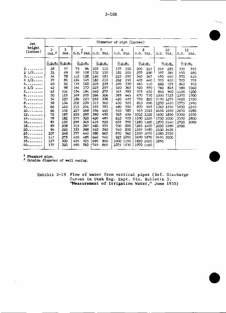
3 -108 .... ....

\

J e t height (inches )

2 ......... 2 l/2 ..... 3 ......... 3 1/2 ..... 4 ......... 4 1/2 .... 5 ......... 6 ......... 7 ......... 8 ......... 9 ......... 10 ........ 12 ........ 14 ........ 16 ........ 18 ........ 20 ........ 25 ........ 30 ........ 35 ........ 40 ........

2 Std . G.p.m.

28 31 34 37 40 42 45 50 54 58 -62 66 72 78 83 89 94 107 117 127 137

3 Std . - :.p.m 57 69 78 86 92 98 10.4 115 125 134 143 152 167 182 195 208 220 2a 275 300 320 .

4 0 . D . Std .

G.p.m.

75 86 95 108 112 128 124 145 135 160 144 173 154 184 169 205 186 223 202 239 215 254 227 268 255 295 275 320 295 345 315 367 333 388 377 440 420 Ce5 455 525 490 565

2 Standard pipe . Gutside diameter o f well casing .

Diameter of pipe (inches)

5 O.D. Std .

G.p.m.

103 115 132 150 160 183 163 210 205 235 225 257 240 275 266 306 293 336 315 360 335 383 356 405 390 450 420 485 455 520 480 555 510 590 580 665 640 740 695 800 745 865

6 3.D. S t d .

G.p.m.

137 150 182 205 225 250 262 293 295 330 320 365 345 395 385 445 420 485 450 520 480 550 510 585 565 650 610 705 655 755 700 800 740 850 830 960 925 1050

LOO0 1150 LO75 1230

8 O.D. Std .

G.p.m.

200 215 275 290 340 367 405 440 465 510 520 570 575 630 670 730 750 820 810 890 870 955 925 1015 1010 1120 1100 1220 1180 U O O 1265 1400 1335 1480 1520 1670 1690 1870 1820 2020 1970 2160

10 O.D. s ta .

G.p.m.

265 265 357 385 450 490 555 610 660 725 760 845 840 940 1000 1125 1150 1275 1270 1420 U60 1550 1450 1650 1600 1830 1730 2000 1870 2140 2000 2280 2100 2420 2380 2720 2650 3000 2850

12 O.D. Std .

G.p.m.

330 355 450 480 570 610 705 755 845 910 980 1060 1120 1200 1370 1500 1600 1730 1775 1950 1930 2140 2070 2280 2300 2550 2530 2800 2720 3000 2900

Exhibit 3-19 Flow of water from vertical p i p e s (Ref . Discharge Curves in Utah Eng . Expt . St.a. Bulletin 5 . “Measurement of Irrigation Water ,” June 1955)

3-109

Y (inches )

0.20 .30 .40 .50 .60 .70 .80 .90 1.00 1.20 1.40 1.60 1.80 2.00 2.20

3 .OO 3.30 3.60 3.90 4.20 4.50 4.80

WHENX = G

2 -inch

G.p.m.

18.3 17.6 16.7 15.4 13.7 9.5 6.0

Size of pipe (naminal diameter)

3-inch

C.p .m.

67.7 66.5 65.1 63.6 62.0 60.4 58.4 55 .7 53.1 46.9 40.5 31.9 24.0 17.3 11.8 7.3

4-inch

G.p .m. 180 175 171 166 161 156 150 145 139 128 115 102 90 77 64 52 41 32

13 24

G.p.m.

308 303 298 2 93 287 282 277 271 265 251 237 221 205 187 167 147 127 108 90 65 45 29

5 -inch

-

&inch

G.p.m.

530 518 506 494 482 470 458 446 422 398 373 347 321 295 270 246 223 200 167 137 111

86 64 45

Exhibit 3-20 Flow of water from horizontal pipes (Ref. Purdue Eng. Expt. Bulletin 32, "Measurement of pipe flow by the coordinate method," August 1928) (Sheet 1 of 3 )

3-110

Y (inches )

0.24 .36 .M .60 .72 .84 .96 1.08 1.20 1.80 2.40 3.00 3.60 4.20 4.80 5.40 6.00 6.60 7.20 7.80 8.40

.96 1.08 1.20 1.80 2.40 3.00 3.60 4.20 4.80 5.40 6.00 6.60 7.20 7.80

Exhibit

WHEN X = 6 INCHES

Size of pipe (naminal diameter) -

2-inch

G.D.Ul.

177 146 126 111 100

92 85 79 75 60 5 1 45 40 37 35 32 30 27 25 23 20

157 l4a 139 114 99 87 79 73 68 63 60 57 54 52

3-inch

G.p.m.

3 10 274 247 229 215 202 193 184 175 139 119 105 94 86 79 71 63 50 38 29

--I-._-

4 -inch

G.p.m.

548 503 462 435 404 377 355 337 319 265 229 206 188 169 151 133 116 99 83 69

WHEN X = 12 INCHES

5 -inch

G.p.m.

969 857 772 705 646 606 574 543 449 3 90 350 314 278 238 193 150 112

319 305 292 247 215 193 176 161 149 140 132 126 120 114

570 548 530 &4 395 359 332 305 287 269 256 242 233 224

1014 974 92 5 763 655 583 530 489 458 426 404 386 368 355

6-inch

G.p.m.

1243 11u 1019 947 $89 w4 808 772 660 583 525 476 43 1 386 332 247

~~

. .. -

1315 12' I 1655

5,?3 1344 772 710 673 633 597 574 5 . a 525

3-20 Flow of water from horizontal pipes (Ref, Purdue En&. Expt. Bulletin 32, "Measurement af p ipe flow by the coordinate method," August 1928) (Sheet 2 of 3 )

Y (inches)

1.80 2.40 3.00 3.60 4.20 4.80 5.40 6.00

1 6.60 7.20 7.80 8.40

3-111

WHEN X = 18 INCHES

2 -inch

G.p.m.

166 1-44 129 117 109 101 95 89 84 81 77 75

Size of pipe (nominal diameter)

3-inch

G,p .m. 346 305 274 251 233 220 206 197 187 180 172 166

4-inch

G.p.m.

624 557 503 4.62 431 404 382 3% 346 332 319 305

5 -inch

G.p.m.

1014 907 826 754 700 655 615 579 548 521 498 476

6-inch

G.p.m. 1400 1261 1153 1068 992 934 884 839 799 763 732 705

Exhibit 3-20 Flow of water from horizontal pipes (Ref. Purdue Eng. Expt. Bulletin 32, "Measurement of pipe flow by the coordinate method," August 1928) (Sheet 3 of 3 )

3-112

Chapter 3

References

1.

2 .

3 .

4 .

5.

6.

Handbook of Hydraulics, King & Brater, Fifth Edition

Hydraulic Charts f o r the Selection of Highway Culverts, Hydraulic Engineering Circular No. 5 , Bureau of Public Roads, Department of Transportation

Hydraulic and Excavation Tables, U. S. Department of Interior, Bureau of Reclamation

Hydraulic Tables, U. S. Department of Defense, Corps of Engineers

Chow, VenTe; Open-Channel Hydraulics, McGraw-Hill Book Co., Inc., 1959

National Engineering Handbook, Section 5, Hydraulics

In addition to the above references, liberal use was made of material from the following references:

a. Hydraulics Correspondence Course by George A. Lawrence, State Conservation Engineer, State of Utah

b. Utah State Engineering Handbook, Section 5 , Hydraulics

c . Vinnard, J. K.; Elementary Fluid Mechanics, John Wiley and Sons , Inc., 1948

chapter 3. · pdf fileengineering fieis manual chapter 3. hydraulics compiled by: william 5....

Documents