chapter 3 multivariate nonparametric regressionkooperberg.fhcrc.org/papers/2009xu.pdfchapter 3...

Chapter 3Multivariate Nonparametric Regression

Charles Kooperberg and Michael LeBlanc

As in many areas of biostatistics, oncological problems often have multivariate pre-dictors. While assuming a linear additive model is convenient and straightforward,it is often not satisfactory when the relation between the outcome measure and thepredictors is either nonlinear or nonadditive. In addition, when the number of predic-tors becomes (much) larger than the number of independent observations, as is thecase for many new genomic technologies, it is impossible to fit standard linear mod-els. In this chapter, we provide a brief overview of some multivariate nonparametricmethods, such as regression trees and splines, and we describe how those methodsare related to traditional linear models. Variable selection (discussed in Chapter 2)is a critical ingredient of the nonparametric regression methods discussed here; be-ing able to compute accurate prediction errors (Chapter 4) is of critical importancein nonparametric regression; when the number of predictors increases substantially,approaches such as bagging and boosting (Chapter 5) are often essential. There areclose connections between the methods discussed in Chapter 5 and some of themethods discussed in Section 3.8.2. In this chapter, we will briefly revisit those top-ics, but we refer to the respective chapters for more details. Support vector machines(Chapter 6), which are not discussed in this chapter, offer another approach to non-parametric regression.

We start this chapter by discussing an example that we will use throughout thechapter. In Section 3.2 we discuss linear and additive models. In Section 3.3 we gen-eralize these models by allowing for interaction effects. In Section 3.4 we discussbasis function expansions, which is a form in which many nonparametric regres-sion methods, such as regression trees (Section 3.5), splines (Section 3.6) and logicregression (Section 3.7) can be written. In Section 3.8 we discuss the situation inwhich the predictor space is high dimensional. We conclude the chapter with dis-cussing some issues pertinent to survival data (Section 3.9) and a brief general dis-cussion (Section 3.10).

C. KooperbergDivision of Public Health Sciences, Fred Hutchinson Cancer Research Center, 1100 Fairview AveN, M3-A410 Seattle, WA 98109-1024, USAemail: [email protected]

X. Li, R. Xu (eds.), High-Dimensional Data Analysis in Cancer Research, Applied 35Bioinformatics and Biostatistics in Cancer Research, DOI 10.1007/978-0-387-69765-9 3,c© Springer Science+Business Media LLC 2009

36 C. Kooperberg and M. LeBlanc

3.1 An Example

We illustrate the methods in this chapter using data from patients diagnosed withmultiple myeloma, a cancer of the plasma cells found in the bone marrow. Thedata were obtained from three consecutive clinical trials evaluating aggressivechemotherapy regiments in conjunction with autologous transplantation conductedat the Myeloma Institute for Research and Therapy, University of Arkansas for Med-ical Sciences (Barlogie et al., 2006). The outcome for patients with myeloma isknown to be variable and is associated with clinical and laboratory measures (Greippet al., 2005). In this data set, potential predictors include several laboratory measuresmeasured at the baseline of the trials, age, gender, and genomic features, includinga summary of cytogenetic abnormalities and approximately 350 single nucleotidepolymorphisms (SNPs) for candidate genes representing functionally relevant poly-morphisms playing a role in normal and abnormal cellular functions, inflammation,and immunity, as well as for some genes thought to be associated with differentialclinical outcome response to chemotherapy.

In most of our analysis we analyze the binary outcome whether there was dis-ease progression after 2 years, using the laboratory measures, age, and gender aspredictors. In Sections 3.7 and 3.8 we also analyze the SNP data; in Section 3.9 weanalyze time to progression and survival using a survival analysis approach.

3.2 Linear and Additive Models

Let Y be a numerical response, and let x = (x1, . . . ,xp)′ be a set of predictors span-ning a covariate space X . We assume that the regression model Y takes the form ofa generalized linear model

g(E(Y |x)) = η(x), (3.1)

where g(·) is some appropriate link function and

η(x) = β0 +k

∑i=1

βixi. (3.2)

In this chapter, we mostly assume that Y is a continuous random variable and thatg(·) is the identity function so that (3.1) is a linear regression model or that Y is abinary random variable and that g(·) is the logit function so that (3.1) is a logisticregression model, but most of the approaches that are discussed in this chapter arealso applicable to other generalized linear models. In Section 3.9, we discuss somemodifications that make these approaches applicable to survival data.

Estimation via the method of maximum likelihood (or least squares) is well es-tablished. Many nonparametric regression methods generalize the model in (3.2).

3 Multivariate Nonparametric Regression 37

In particular, we can replace the linear functions xi in (3.2) by smooth nonlinearfunctions fi(xi). Now (3.2) becomes

η(x) = β0 +k

∑i=1

fi(xi). (3.3)

The functions fi(·) are usually obtained by local linear regression (loess, e.g.,Loader, 1999) or smoothing splines (e.g., Green and Silverman, 1994). The model(3.3) is known as a generalized additive model (Hastie and Tibshirani, 1990).

3.2.1 Example Revisited

Of the 778 subjects with complete covariate data in the multiple myeloma data,171 subjects had progressed after 2 years while 570 subjects had not. Another 37subjects were censored sufficiently early that we chose not to include them in ouranalysis to retain a binary regression strategy. These 37 subjects are included inthe survival analysis (Section 3.9). We used nine predictors: age, gender, lactate de-hydrogenase (ldh), C-reactive protein (crp), hemoglobin, albumin, serum β2 mi-croglobulin (b2m), creatnine, and anyca (an indicator of cytogenetic abnormality).The transformed values of ldh, crp, b2m, and creatnine on the logarithmic scale wereused in the analysis. In a linear logistic regression model, anyca has a Z-statistic of4.8 (p = 10−6), log(b2m) has a Z-statistic of 2.7 (p = 0.007), and log(ldh), albumin,and gender are significant at levels between 0.02 and 0.04.

We then proceeded to fit a generalized additive model, using a smoothing splineto model each of the continuous predictors. We used the R-function gam(), whichselects the smoothing parameter using generalized cross-validation, and providesapproximate inference over the “significance” of the non-nonlinear components.Three predictors were deemed significantly nonlinear at p = 0.05: age, log(crp),and log(b2m), all at significance levels between 0.015 and 0.05. Note that thesesignificance levels are approximate, and they should be treated with caution. Themost interesting significant nonlinearity was probably in log(b2m). In Figure 3.1we show the fitted component with a band of width twice the approximate standarderrors. It appears that the effect of log(b2m) is only present when log(b2m) is above1, which is approximately the median in our data set.

3.3 Interactions

Nonadditive regression models (models for η(x) containing effects of interactionsbetween predictors) occur frequently in oncology. Such models may be needed be-cause additive models, as discussed above, may not provide an accurate fit to thedata, but they may also be of interest to answer specific questions. For example,models containing interactions may be used to identify groups of patients that are


−2 −1 0 1 2 3 4

−2

02

46

log(b2m)

f(lo

g(b2

m))

Fig. 3.1 The component of log(serum β2 microglobulin) in the generalized additive model forprogression after 2 years in the multiple myeloma data.

at especially high or low risk (e.g., LeBlanc et al., 2005), they may be of interest toidentify subgroup effects in clinical trials (e.g., Singer, 2005), or to identify gene ×environment interactions (e.g., Board on health sciences policy, 2002).

In the following several sections, we will discuss general models for interactionsin a regression context. There are, however, special cases in which dedicated meth-ods are more appropriate. For example, if the goal is to only identify patients atespecially high risk, we may not feel a need to model the risk (regression function)for patients at low risk accurately (LeBlanc et al., 2006). When we know that somepredictors are independent of each other, as is sometimes the case for gene × envi-ronment interactions or for nested case–control studies within clinical trials, moreefficient estimation algorithms are possible (Dai et al., 2008). We will not discussthese situations in this chapter.

The most straightforward interaction model is to include all linear interactions upto a particular level in model (3.2); for example, a model with two- and three-levelinteractions is

η(x) = β0 +k

∑i=1

βixi + ∑1≤i< j≤k

βi jxix j + ∑1≤i< j<l≤k

βi jlxix jxl .

It is clear that with this approach the number of coefficients becomes very largequickly. The problems that this causes are even worse when we generalize thesmooth model (3.3). This explosion of the size of the model is sometimes knownas the “curse of dimensionality,” and it can be formalized by establishing the con-vergence rates of parameters in such models under appropriate conditions (Stone,1994). Instead we may want to include only those interactions that are really neededto accurately model the regression function η(x). Often this is done using some formof stepwise regression. It turns out that approach can be generalized convenientlyusing a basis function approach.


3.4 Basis Function Expansions

The linear model (3.1) can also be used as the starting point for nonlinear, nonaddi-tive, multivariate regression methods. Assume that the regression function η(x) isin some p-dimensional linear space B(X ), and let B1(x), . . . ,Bp(x) be a basis forB(X ). Then we can write

η(x) =p

∑i=1

βiBi(x). (3.4)

For a given set of basis functions B1(·), . . . ,Bp(·) estimation in (3.4) is a straightfor-ward extension of (3.2).

Several nonparametric multivariate regression methodologies use a basis func-tion approach, but rather than fixing the space B(X ) these approaches selectthe space at the same time as the coefficients of the basis functions are esti-mated. Three of the methodologies that are discussed later in this chapter use thisapproach.

• Regression tree methods, such as classification and regression trees (CART,Breiman et al., 1984). The basis functions that are used for tree methods areindicator functions corresponding to rectangular regions of the predictor space.Tree methods are discussed in Section 3.5.

• Multivariate adaptive regression splines (MARS, Friedman, 1991) and relatedspline methods (e.g., Kooperberg et al., 1995; Stone et al., 1997). The basis func-tions that are used for MARS and related methods are piecewise polynomials(splines) and their tensor products. We discuss spline methods in Section 3.6.

• Logic regression (Ruczinski et al., 2003) is discussed in Section 3.7. The basisfunctions that are used for logic regression are Boolean combinations of binarypredictors.

Stepwise regression methods provide useful tools for model selection using ba-sis functions. As an example, suppose that we consider two linear spaces to modelη(x): a p-dimensional space Bp(X ) that is a sub-space of a (p+1)-dimensionalspace Bp+1(X ). After we fit model (3.4) using basis functions for the smaller spaceBp(X ) we can compute a score test (Rao statistic, Rao, 1973) to evaluate how muchbetter η(x) would be modeled if we would require that η(x) ∈ Bp+1(X ) instead.Similarly, after we fit model (3.4) using basis functions for the larger space Bp+1(X )we can compute a Wald statistic to evaluate how much worse η(x) would be mod-eled if we would require that η(x) ∈ Bp(X ). If these would be prespecified spacesthe score and Wald statistics could be compared with standard parametric distribu-tions, similar to what is done in stepwise variable selection methods (see Chapter 2).The adaptivity of these approaches does typically require other approaches to obtainsignificant levels and prediction errors though (see Chapter 4).

We can generalize this stepwise procedure to an algorithm for stepwise modelbuilding, that is used both in tree and in spline methods.


1. Start with modeling η(x)∈Bpa . A common situation is that p = 1 and B1

a consistsof only constant functions.

2. Stepwise addition: replace Bpa by a (p + 1)-dimensional space Bp+1

a of whichBp

a is a subspace by considering a (large) set of candidate spaces Bp+1a

that satisfy some method-dependent regularity conditions. Select the “best”Bp+1

a for example, by selecting the Bp+1a corresponding to the largest score

statistic.3. Continue adding dimensions until either a prespecified dimension p∗ is reached,

or until the improvement in the fit between successive models becomes verysmall.

4. Set Bp∗d = Bp∗

a .5. Proceed with stepwise deletion: replace Bp

d by a (p− 1)-dimensional subspaceBp−1

d that satisfies some method-dependent regularity conditions. Select the“best” Bp−1

d , for example, by selecting the candidate corresponding to the small-est Wald statistic.

6. Continue until p reaches some minimum dimension (e.g., p = 1).7. Out of all the linear spaces considered B1

a, . . . ,Bp∗a = Bp∗

d , . . . ,B1d , select one

either using some penalized likelihood like the Akaike information criterion(Akaike, 1974) or the Bayesian information criterion (BIC, Schwarz, 1978), oran honest method to estimate the prediction error, such as cross-validation.

3.5 Regression Tree Models

3.5.1 Background

Regression and classification trees are primarily known for their easy-to-understandgeometric representation. While a binary regression tree provides a simple descrip-tion of groups of subjects, the model can also be cast in a regression spline form sim-ilar to the methods presented in Section 3.6. The CART algorithm (Breiman et al.,1984) is probably the best-known implementation of tree-based methods in the sta-tistical literature and generally motivates the basics given in this section. There hasalso been extensive research of tree-structured methods in machine learning, forinstance the C4.5 algorithm of Quinlan (1993). When extended to survival data, re-gression trees have found a significant following in medicine because the sequenceof binary decisions leads to simple representation for prognostic groups of patientstreated in a similar fashion. Most tree-based methods for survival data have adoptedat least some aspects of the CART algorithm (Gordon and Olshen, 1985; Ciampiet al., 1986; Segal, 1988; LeBlanc and Crowley, 1993). Some recent examples insurvival analysis using regression trees include Greipp et al. (2005), London et al.(2005), Farag et al. (2006), and Gimotty et al. (2007).


3.5.2 Model Building

3.5.2.1 Model Basis Set as Partition Function

A tree model can be represented as a binary tree T , where the set of terminal nodes ˜Tcorresponds to the partition of the covariate space X into a number of M(˜T ) disjointsubsets. A tree model can also be expressed by a basis function representation

η(x) = ∑h∈˜T

ηhBh(x),

(compare with (3.4)) where Bh(x) = I{x ∈ Rh}, Rh is the region corresponding to aterminal node h, and ηh is a vector of parameters (e.g., a mean, a clinical responseprobability, or a higher-dimensional object such as a survival function S(t|η(x))corresponding to a terminal region. For instance, the survival function could be ofsemiparametric form S0(t)exp(η(x)) as in the proportional hazards model. We outlineimportant components of algorithms used to construct regression trees, includingspecifying the types of partitions that are permitted; rules to prune the tree back;and methods to choose model or tree size.

3.5.2.2 Splitting or Basis Selection

Trees represent a sequence of splits of the data or predictor space where each split isinduced by a rule of the form “x ∈ S” where S ⊂ X . Typically, splits are dependenton a single covariate, so we may have S = {x : x j ≤ c} for an ordered predictor, orS is a subset S ⊂ B = {v1,v2, ...,vr} of the r values of x j for categorical variables.

The tree model is grown in a forward stepwise fashion, similar to the stepwisealgorithm described in Section 3.4. Starting with the entire data set and predictorspace, each variable and potential split point is evaluated. The split point and vari-able that leads to the “best” split (as described below) is chosen. The data and thepredictor space are partitioned into two groups. The same algorithm is then recur-sively applied to each of the resulting groups. Therefore, at any point on the regres-sion tree, a split at a node h yields two nodes which can also be represented with thepair of basis functions

b+h( j)(x) = I{xh( j) ∈ Sh( j)} and b−h( j)(x) = I{xh( j) /∈ Sh( j)}.

Each step in the growing process geometrically replaces a current node h with a leftand right daughter nodes l(h) and r(h) or equivalently a current basis function Bh(x)for node h with the basis functions

Bl(h)(x) = Bh(x)b+h( j)(x) and Br(h)(x) = Bh(x)b−h( j)(x).

Most tree algorithms use error, likelihood, or partial likelihood (or score tests suchas the logrank test) to select split points (or knots). The improvement for a split atnode h into left and right daughter nodes can be represented by


G(h) = D(h)− [D(l(h))+D(r(h))],

where D(h) is the residual error at a node. For uncensored continuous responseproblems, D(h) is typically the mean residual sum of squares or mean absoluteerror or for binary data it is typically binomial deviance. For survival data, it wouldbe reasonable to use the deviance corresponding to the assumed survival model. Forinstance, the exponential model deviance for node h is

D(h) = ∑2

[

δi log

(

δi

λhti

)

− (δi −λhti)

]

,

where δi = 1 if the ith observation was a failure, and δi = 0 if the observation wascensored, and λh is the maximum likelihood estimate of the hazard rate in node h(Davis and Anderson, 1989). Alternatively G(h) can be an appropriate score teststatistic, for example the logrank test statistic.

Typically a large tree is grown to avoid missing structure and then pruned backusing a method described below.

3.5.3 Backwards Selection (Pruning)

Many stepwise regression methods utilize variations of backwards selection to selectmore simple models (see Section 3.4). The local nature of the tree-based methodsleads to a fast backwards method, called cost complexity pruning in the CART algo-rithm, for evaluating all possible submodels. The cost-complexity objective functionis defined as a penalized measure of fit

Dα(T ) = ∑h∈˜T

D(t)+αM(˜T ),

where α is a nonnegative complexity parameter, D(h) is the estimated cost or im-purity of a node, and M(˜T ) is the number of terminal nodes or constant regressionregions Rh. Therefore, the cost-complexity measure controls the trade-off betweenthe size or complexity of the tree, and how well the tree fits the data. Then, for anyvalue of α the goal is to find T (α): the tree that minimizes Dα(T ) among all prunedsubtrees of T . The algorithm finds the sequence of optimally pruned subtrees byrepeatedly deleting branches of the tree for which the average reduction in resid-ual error per split in the branch is small. The process yields a nested sequence ofoptimal subtrees T (α) = T (αl) = Tl for αl ≤ α < αl+1. The removal of a branchcan again be viewed in regression context as replacing each of the basis functionscorresponding to the pruned branch with the sum of the basis functions

Bl(x) = ∑h∈Ql

Bh(x)


where Ql represent the nodes in a branch rooted at node l. The final tree size isselected by resampling (often K-fold cross-validation is used), although some diffi-culties arise for semiparametric survival regression models.


Using the example data set and variables described earlier, we constructed a regres-sion tree to characterize the probability of death or progression within 2 years of reg-istration. Figure 3.2 show a large tree constructed on the available predictors. Beloweach terminal node is an estimate of the probability of progression or death. Sincethe tree likely over-fits the data, a pruned tree is selected using cost-complexitypruning and ten fold cross-validation of binomial deviance. The resulting treemodel is presented in Figure 3.3; it includes just two splits on variables serum β2

b2m<10.2

ldh<222

age<67.8

ldh<160

crp<25.3

albumin<3.6

0.235 0.560

0.2930.163 0.552

0.654 0.320

Fig. 3.2 An unpruned regression tree constructed to characterize 2-year progression probabilityfor the multiple myeloma data.

b2m<10.2

ldh<222

0.184 0.365

0.490

Fig. 3.3 A pruned regression tree constructed to characterize 2-year progression probability forthe multiple myeloma data.


microglobulin and lactate dehydrogenase and identifies three outcome groups. Sub-jects with serum β2 microglobulin ≥ 10.2 have the worst outcome with 49% havingeither progressed or died within 2 years.

3.5.5 Issues and Connections

An often cited limitation of regression trees is that they are piecewise constant func-tions when typically the underlying conditional distribution function of the outcomeis a smooth function of the predictors. If interest is in studying groups of patients,this is not really a problem, other than the difficulty in specifying a specific frac-tion of patients to be indicated by the prognostic rule. However, for predictionapplications the nonsmoothness does lead to reduced performance. Ensembles oftrees, through boosting, bagging, and Random Forests (Freund and Schapire, 1996;Breiman, 1996; Friedman et al., 2000) have been used to circumvent this discrete-ness at the cost of losing the simple decision rules. Alternatively, spline methodssuch as HARE or MARS described in Section 3.6 can lead to substantially improvedpredictions.

In part because of their nonsmoothness and the stepwise selection method, treesare subject to considerable variability. An important parameter to control variabilityis the minimum number of observations in a node (or uncensored observations in thecase of censored survival data). This issue connects to the importance of avoidingplacing knots in regression splines too close to the edge of the covariate distribution.Again, ensembles of trees have been used to reduce variability (sometimes dramati-cally) but again at the loss of the simple decision rule properties. Retaining decisionrule but somewhat smoother methods have been proposed, such as rule inductionvia the PRIM method (Friedman and Fisher, 1999).

3.6 Spline Models

3.6.1 One Dimensional

Spline models are primarily used for the approximation of smooth univariate andmultivariate functions. In univariate problems, splines are piecewise polynomialfunctions, that satisfy some regularity conditions. In particular, let t0 < t1 < · · ·< tKbe a set of K knots. A function f (x) is a cubic spline if in each of the intervals(tk−1, tk), k = 1, . . . ,K, the function f (x) is a cubic polynomial, and it is twice dif-ferentiable everywhere. Different spline models may have boundary restrictions forf (x) on the intervals (−∞, t0] and [tK ,∞), but when there are no boundary conditionsit is easy to see that these cubic spline functions form a linear space, with basis

1,x,x2,x3,(x− tk)3+, k = 0, . . . ,K, (3.5)


0 1 2 3 4 5 6

−1.

5−

0.5

0.0

0.5

1.0

1.5

−1.

0

f(x)

spline

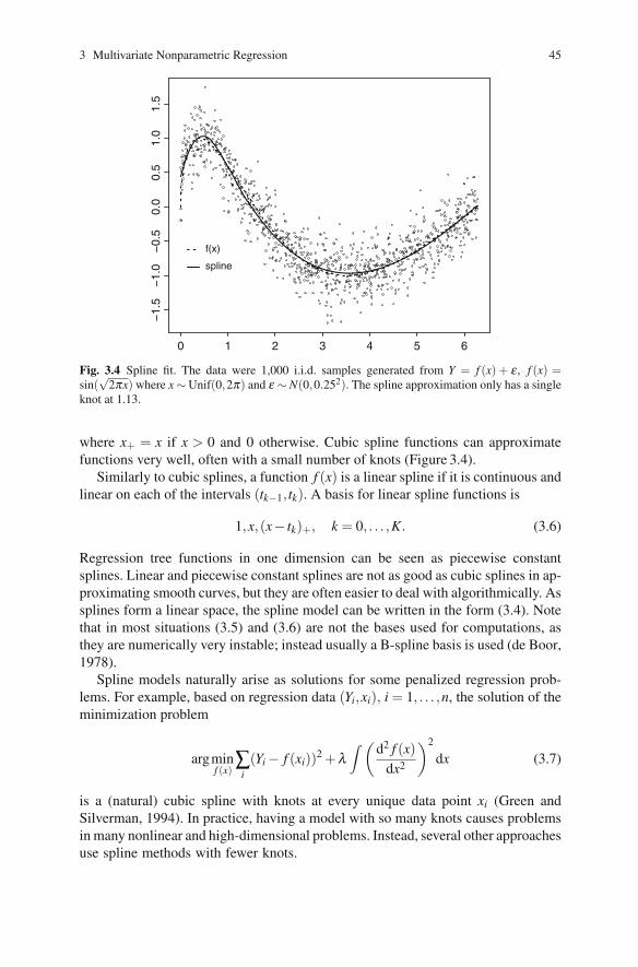
Fig. 3.4 Spline fit. The data were 1,000 i.i.d. samples generated from Y = f (x) + ε , f (x) =sin(

√2πx) where x ∼ Unif(0,2π) and ε ∼ N(0,0.252). The spline approximation only has a single

knot at 1.13.

where x+ = x if x > 0 and 0 otherwise. Cubic spline functions can approximatefunctions very well, often with a small number of knots (Figure 3.4).

Similarly to cubic splines, a function f (x) is a linear spline if it is continuous andlinear on each of the intervals (tk−1, tk). A basis for linear spline functions is

1,x,(x− tk)+, k = 0, . . . ,K. (3.6)

Regression tree functions in one dimension can be seen as piecewise constantsplines. Linear and piecewise constant splines are not as good as cubic splines in ap-proximating smooth curves, but they are often easier to deal with algorithmically. Assplines form a linear space, the spline model can be written in the form (3.4). Notethat in most situations (3.5) and (3.6) are not the bases used for computations, asthey are numerically very instable; instead usually a B-spline basis is used (de Boor,1978).

Spline models naturally arise as solutions for some penalized regression prob-lems. For example, based on regression data (Yi,xi), i = 1, . . . ,n, the solution of theminimization problem

argminf (x)

∑i(Yi − f (xi))2 +λ

∫(

d2 f (x)dx2

)2

dx (3.7)

is a (natural) cubic spline with knots at every unique data point xi (Green andSilverman, 1994). In practice, having a model with so many knots causes problemsin many nonlinear and high-dimensional problems. Instead, several other approachesuse spline methods with fewer knots.


• Instead of using n knots, express f (x) as a spline function with a fairly largenumber of knots, that is still much smaller than n, and then use a penalized op-timization like (3.7) (O’Sullivan, 1988; Eilers and Marx, 1996). This approachworks fairly well in more complicated one-dimensional problems, as well as forgeneralized additive models, in particular with automatic rules to select smooth-ing parameters.

• Use a much smaller number of pre-specified knots, and carry out estimation with-out penalty terms. The advantage is that the resulting problem is fully paramet-ric, and that inference is thus well established. Estimation problems are oftensmall (and easy). See Quantin et al. (1999) for an application in oncology. Thedisadvantage is that selection of the location of the knots can be arbitrary, andgeneralizations to nonadditive models are not immediate.

• A third alternative is to use a stepwise algorithm like the one described in Sec-tion 3.4 using knots and basis functions from (3.5). This approach was first usedin univariate regression by Smith (1982) and is behind algorithms like MARS(Friedman, 1991) for linear regression, HARE (Kooperberg et al., 1995) for sur-vival data, and Polyclass (Kooperberg et al., 1997) for logistic regression andclassification. We will discuss those in more detail for multivariate models be-low. See Polesel et al. (2005) for an application in oncology.

3.6.2 Higher-Dimensional Models

The common approach to using regression splines in higher dimensions is to usebasis functions that are tensor products of basis functions in one dimension. For ex-ample, if B1(x) = g1(xk) and B2(x) = g2(xl) are two basis functions that depend ona single predictor, then B3(x) = g1(xk)g2(xl) is a tensor product basis function thatdepends on two predictors. For high-dimensional problems, it is common to con-sider only a few selected lower-order interactions. This has a variety of advantages:(1) lower-dimensional components are typically easier to interpret, interactions inmodels that do not contain the corresponding main effects are particularly difficult tointerpret; (2) using all (higher order) tensor products of lower-order basis functionswould yield an extremely large number of basis functions and may cause numericalinstability, and (3) from a theoretical perspective, it has been established that splinefunctions have faster convergence rates if the largest order of interactions in modelsis small (Stone, 1994). The exact restrictions on when tensor product basis functionsare allowed in spline models differs from one methodology to the other: for exam-ple, MARS (Friedman, 1991) has fewer restrictions than HARE (Kooperberg et al.,1995), Polyclass, and Polymars (Kooperberg et al., 1997). Here we will describe thePolyclass algorithm for logistic regression as an example.

Assume that we have an i.i.d. sample of size n with a binary response vari-able Y and a p-dimensional vector of predictors x = (x1, . . .xp)′. Polyclass useslinear splines, and uses interactions involving at most two predictors (althoughthe generalization to higher-dimensional interactions is immediate). An allowable


linear space B(§) can have basis functions 1, xi, (xi − tki)+, xix j, (xi − tki)+x j, and(xi − tki)+(x j − tk j)+, with i �= j ∈ {1, . . . , p}, where the tki are knots in the range ofxi, with the additional conditions that

• B(x) = xix j can only be in B(§) if B(x) = xi and B(x) = x j are in B(§);• B(x) = (xi − tki)+ can only be in B(§) if B(x) = xi is in B(§);• B(x) = (xi − tki)+x j can only be in B(§) if B(x) = xix j and B(x) = (xi − tki)+ are

in B(§); and• B(x) = (xi − tki)+(x j − tk j)+ can only be in B(§) if B(x) = xi(x j − tk j)+ and

B(x) = (xi − tki)+x j are in B(§).The algorithm then proceeds with the stepwise algorithm in Section 3.4. The finalmodel is selected as the one that minimizes

AICα = −�(B(§);Yi,xi, i = 1, . . . ,n)+α p, (3.8)

where �(B(§);Yi,xi, i = 1, . . . ,n) is the fitted log-likelihood for one of the models (ofdimension p) that was considered, and α is a penalty parameter, or that maximizesthe cross-validated likelihood.


We applied the Polyclass methodology to the multiple myeloma data. The polyclassmodel with the default penalty parameter of α = logn ≈ 6.66 (3.8) only involvedthe two predictors log(b2m) and anyca in a linear fashion:

logit(P(progression)) = 2.19−0.99log(b2m)−0.50anyca.

The model with α = 4, while likely overfitting the data somewhat, is more interest-ing, as it also involves age, gender, log(ldh), log(creatinine), a knot in age, log(ldh),and log(b2m), and an interaction between age and gender. In Figure 3.5 we show acontour plot for the fitted 2-year progression probabilities as a function of creatinineand age, separately for men and women, when the other predictors are held at theirmedian values. The figure indicates that while older ages lead to quite similar pro-gression proportions, younger females tend to have higher risk than younger males.

3.7 Logic Regression

Logic regression is a generalized regression methodology that is particularly suitedfor situations in which (most) predictors are binary. Clearly this is the case whenpredictors are single nucleotide polymorphisms (SNPs), as is the case for themultiple myeloma data and many other oncological problems. The logic regressionmodel is


age

crea

tinin

e

40 50 60 70 40 50 60 70

13

1030

men

age

women

Fig. 3.5 Fitted 2-year progression probabilities for a Polyclass model selected with penalty α = 4as a function of creatinine and age, separately for men and women, when the other predictors areheld at their median values.

η(x) = β0 +m

∑i=1

βiLi(x). (3.9)

Each of the Li is a Boolean combination of binary predictors x j, j = 1, . . . ,J such as

Li = [(x7 and xc13) or x5],

where “1” equals “true,” “0” equals “false,” and c refers to the complement. Ad-ditional predictors Z or components to correct for population stratification can beincluded additively in model (3.9).

Logic regression is an adaptive algorithm which selects those logic terms Li thatminimize the residual sum of squares or maximize the log-likelihood correspondingto the model (3.9). Typically in logic regression the number of logic terms m is small(between 1 and 3), and the logic terms can be interpreted as “risk factors.” Theoptimization of the logic regression model is carried out using a greedy stepwisealgorithm or a stochastic simulated annealing algorithm.

For this simulated annealing algorithm it turns out to be very convenient to repre-sent a logic expression Li(x) in a logic tree form (Figure 3.6). During the simulatedannealing algorithm, at each step one of the logic trees is replaced by another logictree using one of the operations displayed in Figure 3.7. Based on the new tree thelikelihood of η(x) is evaluated. If the new model is an improvement over the exist-ing model the new model is retained; if the old model was better the new model isretained with a probability that depends on the difference between the old and newlog-likelihood and the stage of the algorithm: early on almost all new models are ac-cepted, while toward the end of the algorithm only improved models are accepted.


1 4

1 2 3 or

and and

or

Fig. 3.6 A logic tree representation of the Boolean expression (x1 ∧ xc2)∨ (x3 ∧ (xc

1 ∨ x4)). Logictrees are evaluated from the bottom up; white numbers on a black background denote thecomplement.

Possible Moves

4 3

1 or

and

Alternate Leaf

(a)

2 3

1 or

or

Alternate Operator

(b)

2 3

5 or

1 and

and

Grow Branch

(c)

2 3

1 or

and

Initial Tree

2 3

or

Prune Branch

(d)

3 6

2 and

1 or

and

Split Leaf

(e)

1 2

and

Delete Leaf

(f)

Fig. 3.7 Changes in logic regression trees considered during the simulated annealing algorithm.


We applied logic regression to the 348 SNPs of the multiple myeloma data, usingagain 2-year progression as the outcome. Each of the 348 SNPs was recoded as twobinary predictors corresponding to a dominant and a recessive effect. In Figure 3.8


0 1 2 3 4

800

850

900

950

model size

test

sco

res

01

1 1

1/2

2

2

Fig. 3.8 Cross-validation (test set) deviance for the logic regression analysis of the multiplemyeloma data. The white numbers in the black squares refer to the number of logic terms inthe logic regression model, the model size refers to the total number of leaves in these modelscombines.

we show the test set deviance from tenfold cross-validation of the logic regressionanalysis of this data. We note from this figure that based purely on deviance, noneof the models is better than the null-model. The model with two SNPs, however, hasa deviance that is not much worse than the null-model, and may thus be of interestfor further investigation. This model includes a logic regression term

rs4148737D∨ rs1143627Rc,

(rs1922242D was identical to rs4148737D) on this data. We will see the same SNPsappear in the analysis in the next section.

3.8 High-Dimensional Data

With the development of new genomic technologies, very high-dimensional datasets are now generated for oncological data. Data sets using gene expression datamay have data on tens of thousands of genes (e.g., Rosenwald et al., 2002), data setsfor whole genome association studies may have data on hundreds of thousands ofSNPs (e.g., Easton et al., 2007; Yeager et al., 2007). The traditional statistical para-digm, where the number of cases n is much larger than the number of predictors pno longer holds in this situation. Typical statistical methods for this type of data in-volve substantial amounts of model selection, as well as shrinkage of the parameterestimates.


3.8.1 Variable Selection and Shrinkage

In moderate to high-dimensional predictor settings it is desirable to have parsimo-nious or sparse representations of prediction models. In the previous sections wehave discussed stepwise basis function selection strategies. Alternatively, one caninvestigate smoother model selection methods.

3.8.2 LASSO and LARS

Consider the linear regression setting, where there are n independent observations(yi,xi1, . . . ,xik) of the response and k predictor variables. A technique proposed byTibshirani (1996) introduces an L1-penalty on the regression coefficients which leadsto both shrinkage and variable selection called least absolute shrinkage and selectionoperator (LASSO). This is in contrast to ridge regression (Hoerl and Kennard,1970) which minimizes the residual error subject to an L2-penalty which does notlead to variable selection. The LASSO estimate ˜β = (β1, . . . , ˜βm)′ is defined as theminimizer of

g(β ) =n

∑i=1

(yi −∑k

βkxik)2 +λ1 ∑ |βk|1,

where λ1 is a nonnegative penalty parameter. Often the response and predictors arestandardized so that ∑

iyi = 0 and ∑

ixik = 0 and ∑

ix2

ik = 1. This estimator has the

attractive property that as λ1 increases minimizing g(β ) with respect to β leadsto some of the βk set to zero and hence variable selection. For fixed λ1, for opti-mization quadratic programming techniques or alternatives more efficient methodsby Osborne et al. (2004) can be used. A related and highly efficient algorithm, theleast angle regression algorithm (LARS, Efron et al., 2004), leads to efficient esti-mation and links forward stage-wise methods and LASSO. LASSO and LARS arediscussed in more detail in Chapter 2.

LARS gives answers that are often close to LASSO; they are identical if thepredictors are orthogonal. However, the estimation algorithm aligns closely with theforward stepwise model building strategies described in earlier sections. An outlineof the algorithm is given below:

1. Start with r = y, β j = 0, j = 1, . . . , p. Assume that the x j are standardized.2. Find the predictor xk that is most correlated with r.3. Increase βk in the direction of sign(cor(r,xk)) until another predictor x j has equal

correlation to r as it does with xk. Put j in set of active predictors, S.4. Move (βk : k ∈ S) in the joint least squares direction for (xk : k ∈ S) until yet

another predictor has equal correlation with the current residual.5. Repeat Step 4 until cor(r,xk) = 0 for all k.


Note that the model can include at most min(p,n) variables. One strategy to alle-viate this potential problem is the “elastic net” proposed by Zou and Hastie (2005).The elastic net can be expressed as an optimization problem with the objective func-tion with both squared and absolute penalty terms

g(β ) =N

∑i=1

(yi −∑k

βkxik)2 +λ1 ∑ |βk|1 +λ2 ∑ |βk|2.

Their simulations show that the elastic net method leads to grouping of variableswhere strongly correlated variables are either in or removed from the model as thepenalty parameters λ1 and λ2 are increased.

Note, that in this section we have described these methods in terms of the originalpredictors xk; we could generalize to sets of regression spline or regression tree basisfunctions, B j(x), j = 1, . . . , p as described in the previous section.

3.8.3 Dedicated Methods

While the methods described above directly lead to dimension reduction, there are alarge number of other methods which can be viewed as two-stage procedures that atthe first stage reduce the set of original variables xi to a small number of combina-tions zi and then at the second phase uses those combinations in further regressionmodeling. Many of the techniques can be viewed as generalizations or parallels toeither principal components regression, which uses only the joint distribution of thexi at the first stage, or partial least squares which constructs linear combinations ofthe predictors but also guides the selection by also using the outcome Y .

For instance, many gene expression modeling applications in oncology haveused clustering of genes to derive predictor variables for association modeling.Jointly using outcome and expression was used by Hastie et al. (2001) and Det-tling and Buhlmann (2002) and others. An important consideration when using boththe joint distribution of outcome and predictors at the first stage is that appropriateassessment of prediction error and model fit is incorporated (for instance by cross-validation) and included in the modeling building.


We applied a generalization of the LARS regression method appropriate for binarydata (Park and Hastie, 2006) to the 2-year progression-free survival outcome, andthe multiple myeloma SNP data. Each of the SNPs was coded in dominant andrecessive form. In the Figure 3.9, we show the first few steps of the coefficient path.Three SNPs appear to enter the model early, “rs1143627R,” “rs2756109D,” and“rs703842R.” Note that the SNPs that were selected by logic regression entered


**********************

0.0 0.1 0.2 0.3

−0.

10−

0.08

−0.0

6−0

.04

−0.0

20.

000.

02

|β|

Sta

ndar

dize

d co

effic

ient

s

********************** ********************** ********************** ********************** **************** *

** * * *

********************** ***********************

*

***

***

** * ***

* **

** * * *

********************** *********************** * ** * ***

** * ***

* **

** * * *

********************** ********************** ********************** ********************** ********************** ********************** ********************** ********************** ********************** ********************** ********************** **************

***

** * * *

********************** *********************** * ***

***

** * ***

* **

** * * *

********************** ********************** ********************** ********************** ********************** ********************** ********************** *********************** * ** * *** ** * ***

* **

** * * *

********************** ********************** ********************** ********************** ********************** ********************** ********************** ********************** ********************** ********************** *********************** * ** *

***** * * ** * * *

** * * *

* * ** *

***** * * ** * * *

** * * *

*************** *

*** * * *

* *

***

***

** * ***

* **

** * * *

********************** ********************** ********************** ****************** * * * *********************** ********************** ********************** *********************** * ** * ***

** * ***

* **

** * * *

********************** *****************

** * * *

********************** **********************

rs1143627R

rs2756109D

rs703842R

rs2181874Rrs2808668R

rs238417D

51 SNPsrs2287499Drs4077829R

rs4645943D

rs1922242D/4148737Drs7252741Drs2853749R

1 2 3 4/5 67 8 9 10 11 12 1314

Fig. 3.9 Coefficient path for myeloma SNP data.

the model as the first, fourth, and fifth SNP. Cross-validating the model buildingprocess leads to the conclusion that the cross-validated estimates of deviance arerelatively flat with respect to model complexity and then start to increase for modelswith larger numbers of predictors. Therefore, there is not strong evidence that thecombination of SNPs are significantly associated with disease progression.

Often there is interest in assessing if genomic information adds to predictionbeyond traditional laboratory measures. This can be easily incorporated by adjust-ing for known myeloma clinical variables then fitting SNP data using the Park andHastie algorithm. This was done for the above example and while not unexpectedgiven the earlier analysis, it suggested no additional impact with SNP data on pre-diction over the laboratory variables previously described.

3.9 Survival Data

An important goal in survival regression analysis is to determine how the distribu-tion of survival times depends on the predictors. A complication in analyzing sur-vival data in the context of oncology trials is that typically not all patients have died(or progressed) by the time the analysis for the study is completed. Those patientsalive at the time of analysis are called censored.


We denote the true survival time as a positive random variable T , whose distri-bution may depend on a set of predictors x = (x1, . . . ,xk)′. Often it can be assumedthat the censoring mechanism is independent which facilitates likelihood construc-tion and inference. Let the observed data be denoted by (Ti,δi,xi), i = 1, . . . ,n.

While one can express the conditional survival distribution using an acceleratedfailure time specification which links the log(T ) to a linear model of the predictors,log(T ) = a+b′X +e, hazard function modeling is most often used. The conditionalhazard function is defined as

λ (t|x) = limΔ→0

P(t ≤ T < t +Δ |t ≤ T ;x)Δ

.

Here, we limit discussion to predictors which are real values measured at baseline; insome survival settings they may represent time-dependent functions, x1(t), . . . ,xk(t),as well. For instance, they may be measures of health status of the patient evolvingover time. The (conditional) hazard function can be interpreted as the probabilitythat someone dies in the next time interval of infinitesimal length Δ , given that heis alive at time t. It is convenient to specify models on the logarithm scale so wedenote the logarithm of the hazard function as

α(t|x) = logλ (t|x).

If one assumes an additive model on the log scale,

α(t|x) = f (t)+η(x)

implies a proportional hazards assumption which is a focus of the model of Cox(1972), which also assumes the baseline hazard function to be an unspecified non-parametric function. Estimation in that case utilizes the partial likelihood. Note thatη(x) can represent a simple linear model or more flexible models depending on a re-gression spline basis described in earlier sections. For instance, let B1(x), . . . ,Bp(x)be a basis for B(X ). Then we can write

η(x) =p

∑i=1

βiBi(x). (3.10)

Within the proportional hazards class, tree-based or logic regression models canbe used to characterize the basis section used in the above expression.

However, regression models can be more general. For instance, the HARE model(Kooperberg et al., 1995), can link both time and the predictors using a model spec-ified as

α(t|x) = ∑i

βiBi(t|x). (3.11)

The basis functions Bi(t|x) in HARE can depend solely on time or a predictor orboth on time and a predictor which allows specification on nonproportional hazards


models. The basis functions are selected with an algorithm similar to the Polyclassalgorithm in Section 3.6.2.

Modeling the full survival distribution is slightly more general than modelingwithin the proportional hazards framework. But there are also disadvantages: co-efficients in model (3.10) are interpretable as log-relative risk estimates, while thenonproportionality in (3.11) removes this interpretation. Computationally the partiallikelihood computations for (3.10) are much easier than the full likelihood compu-tations for (3.11), as these later require integrating the conditional survival functionfor every unique set of covariates x which, except for piecewise linear splines, be-comes very demanding.

We end this section by noting that a simple transformation of the survival timesmay facilitate modeling. Suppose that T is a continuous random variable havingdistribution function F . Then U = F(T ) has a standard uniform distribution andlog(U) = Λ(T ), where Λ represents the cumulative hazard function, has a standardexponential distribution and thus a constant hazard function. In the context of haz-ard function modeling with HARE, the regression model applied to survival timestransformed by the marginal cumulative hazard function tends to require fewerknots applied to the time variable allowing more focus on the impact of predictorson the (transformed) outcome. The overall transformation applied to the data can besemiparametric, for instance using a regression spline model for the hazard function(the HEFT method of Kooperberg et al., 1995) or non-parametric using the em-pirical cumulative hazard function estimate. This transformation can facilitate theuse of other flexible regression procedures utilizing exponential model likelihood,which typically allows for much faster computation than partial likelihood. Forinstance, after transforming the survival times by the cumulative hazard transfor-mation, the survival times may be sufficiently well approximated by an exponentialdistribution, so that a regression tree program based on the exponential likelihoodmay perform well.


The multiple myeloma data set included both overall survival and progression-freesurvival endpoint data. In this analysis, we consider all 778 subjects with com-plete covariate data. The HARE analysis of the time to progression is very similarto the Polyclass analysis presented in Section 3.6.3. The analysis of the survivaltime turned out more interesting, as it depended on serum β2 microglobulin, anyca,log(ldh), and age, and included a nonproportionality component for log(ldh). InFigure 3.10, we show the fitted hazard function for a person of age 56, with alog(b2m) of 1, no anyca, and log(ldh) values of 4, 5, and 6, which roughly cor-respond to the 25th, 50th, and 75th percentile of the log(ldh).


0 1 2 3

0.00

10.

003

0.01

0.03

0.1

log(LDH)=4log(LDH)=5log(LDH)=6

time (years)

haza

rd

Fig. 3.10 Fitted hazard functions for the HARE analysis of the multiple myeloma data.

3.10 Discussion

Many choices exist for flexible regression modeling of patient data from oncologystudies. Selection of appropriate methods, of course, depends on the goals in theparticular analysis. For instance, it could be best to characterize the risk of progres-sion as a smooth function of a single important prognostic variable or to develop amore general risk models using multiple predictors and variable selection. Adaptiveregression spline methods such as HARE are well suited to such problems. Alter-natively, one may want to characterize groups of patients or subjects, or identifyinteractions of binary predictor variables. Tree-based methods or logic regressionare two tools useful for such problems.

A common aspect of cancer data is that the strength of associations betweenpredictors and patient outcome is quite weak as demonstrated with the myelomadata. While sometimes it is useful to slightly overfit the data to suggest models thatmay be worth investigating further, in general we should prevent selecting regressionmodels that are not supported by the data. Therefore, using methods to obtain honestprediction error to help avoid over-fitting is critical.

References

Akaike, H. (1974). A new look at the statistical model identification. IEEE Transactions onAutomatic Control, 19:716–723.

Barlogie, B., Tricot, G., Rasmussen, E., Anaissie, E., van Rhee, F., Zangari, M., Fassas, A.,Hollmig, K., Pineda-Roman, M., Shaughnessy, J., Epstein, J., and Crowley, J. (2006). Totaltherapy 2 without thalidomide in comparison with total therapy 1: role of intensified inductionand posttransplantation consolidation therapies. Blood, 107:2633–2638.

Board on health sciences policy. (2002). Cancer and the Environment: Gene–Environment Inter-action. Institute of Medicine, National Academy Press, Washington D. C.


de Boor, C. (1978). A Practical Guide to Splines. Springer-Verlag, New York.Breiman, L. (1996). Bagging predictors. Machine Learning, 24:123–140.Breiman, L., Friedman, J. H., Olshen, R. A., and Stone, C. J. (1984). Classification and Regression

Trees. Wadsworth, Pacific Grove, California.Ciampi, A., Thiffault, J., Nakache, J. P., and Asselain, B. (1986). Stratification by stepwise re-

gression, correspondence analysis and recursive partition. Computational Statistics and DataAnalysis, 4:185–204.

Cox, D. R. (1972). Regression models and life tables (with discussion). Journal of the RoyalStatistical Society B, 34:187–220.

Dai, J. Y., LeBlanc, M., and Kooperberg, C. (2008). Semiparametric estimation exploiting covari-ate independence in two-phase randomized trials. Biometrics, May 12. [Epub ahead of print].

Davis, R. B. and Anderson, J. R. (1989). Exponential survival trees. Statistics in Medicine,8:947–961.

Dettling, M. and Buhlmann, P. (2002). Supervised clustering of genes. Genome Biology, 3:69.1–69.15.

Easton, D. F., Pooley, K. A., Dunning, A. M., Pharoah, P. D. P., Thompson, D., Ballinger, D. G.,Struewing, J. P., Morrison, J., Field, H., Luben, R., et al. (2007). Genome-wide associationstudy identifies novel breast cancer susceptibility loci. Nature, 447:1087–1093.

Efron, B., Hastie, T., Johnstone, I., and Tibshirani, R. (2004). Least angle regression. The Annalsof Statistics, 32:407–499.

Eilers, P. H. C. and Marx, B. D. (1996). Flexible smoothing with B-splines and penalties (withdiscussion). Statistical Science, 11:89–121.

Farag, S., Archer, K. K., Mrozek, K., Ruppert, A. S., Carroll, A. J., Vardiman, J. W., Pettenati,J., Baer, M. R., Qumsiyeh, M. B., Koduru, P. R., et al. (2006). Pretreatment cytogenetics add toother prognostic factors predicting complete remission and long-term outcome in patients 60years of age or older with acute myeloid leukemia: results from Cancer and Leukemia GroupB 8461. Blood, Jul. 1; 108(1):63–73.

Freund, Y. and Schapire, R. E. (1996). Experiments with a new boosting algorithm. InMachine Learning: Proceedings of the Tirteenth International Conference, pp. 148–156.Morgan Kauffman, San Francisco.

Friedman, J. H. (1991). Multivariate adaptive regression splines (with discussion). The Annals ofStatistics, 19:1–141.

Friedman, J. H. and Fisher, N. I. (1999). Bump-hunting for high dimensional data. Statistics andComputation, 9:123–143.

Friedman, J. H., Hastie, T., and Tibshirani, R. (2000). Additive logistic regression: A statisticalview of boosting (with discussion). The Annals of Statistics, 38:337–407.

Gimotty, P. A., Elder, D. E., Fraker, D. L., Botbyl, J., Sellers, K., Elenitsas, R., Ming, M. E.,Schuchter, L., Spitz, F. R., Czerniecki, B. J., and Guerry, D. (2007). Identification of high-riskpatients among those diagnosed with thin cutaneous melanomas. Journal of Clinical Oncology,25:1129–1134.

Gordon, L. and Olshen, R. A. (1985). Tree-structured survival analysis. Cancer Treatment Reports,69:1065–1069.

Green, P. J. and Silverman, B. W. (1994). Nonparametric Regression and Generalized LinearModels: a Roughness Penalty Approach. Chapman and Hall, London.

Greipp, P. R., San Miguel, J., Durie, B. G., Crowley, J. J., Barlogie, B., Blade, J., Boccadoro,M., Child, J. A., Avet-Loiseau, H., Kyle, R. A., et al. (2005). International staging system formultiple myeloma. Journal of Clinical Oncology, 23:3412–3420.

Hastie, T. J. and Tibshirani, R. J. (1990). Generalized Additive Models. Chapman and Hall,London.

Hastie, T., Tibshirani, R., Botstein, D., and Brown, P. (2001). Supervised harvesting of regressiontrees. Genome Biology, 2:3.1–3.12.

Hoerl, A. E. and Kennard, R. W. (1970). Ridge regression: biased estimation for nonorthogonalproblems. Technometrics, 12:55–67.


Kooperberg, C., Stone, C. J., and Truong, Y. K. (1995). Hazard regression. Journal of the AmericanStatistical Association, 90:78–94.

Kooperberg, C., Bose, S., and Stone, C. J. (1997). Polychotomous regression. Journal of theAmerican Statistical Association, 92:117–127.

LeBlanc, M. and Crowley, J. (1993). Survival trees by goodness of split. Journal of the AmericanStatistical Association, 88:457–467.

LeBlanc, M., Moon, J., and Crowley, J. (2005). Adaptive risk group refinement. Biometrics,61:370–378.

LeBlanc, M., Moon, J., and Kooperberg, C. (2006). Extreme regression. Biostatistics, 13:106–122.Loader, C. (1999). Local Regression and Likelihood. Springer-Verlag, New York.London, W. B., Castleberry, R. P., Matthay, K. K., Look, A. T., Seeger, R. C., Shimada, H., Thorner,

P., Broderu, G., Maris, J. M., Reynolds, C. P., and Cohn, S. L. (2005). Evidence for an age cutoffgreater than 365 days for neuroblastoma risk group stratification in the Children’s OncologyGroup. Journal of Clinical Oncology, 23:6459–6465.

Osborne, M. R., Presnell, B., and Turlach, B. A. (2004). On the LASSO and its dual. Journal ofComputational and Graphical Statistics, 9:319–337.

O’Sullivan, F. (1988). Fast computation of fully automated log-density and log-hazard estimators.SIAM Journal on Scientific and Statistical Computing, 9:363–379.

Park, M. Y. and Hastie, T. (2006). L1 regularization path models for generalized linear models.Journal of the Royal Statistical Society B, page in press.

Polesel, J., Dal Maso, L., Bagnardi, V., Zucchetto, A., Zambon, A., Levi, F., La Vecchia, C., andFraneschi, S. (2005). Estimating dose-response relationship between ethanol and risk of cancerusing regression spline models. International Journal of Cancer, 114:836–841.

Quantin, C., Abrahamowicz, M., Moreau, T., Bartlett, G., MacKenzie, T., Tazi, M. A., Lalonde, L.,and Faivre, J. (1999). Variation over time of the effects of prognostic factors in a population-based study of colon cancer: Comparison of statistical models. American Journal of Epidemi-ology, 150:1188–1200.

Quinlan, J. R. (1993). C4.5 Programs for Machine Learning. Morgan Kaufman, San Francisco,CA.

Rao, C. R. (1973). Linear Statistical Inference and Its Applications. John Wiley, New York.Rosenwald, A., Wright, G., Chan, W., Connors, J., Campo, D., Fisher, R., Gascoyne, R., Muller-

Hermelink, H., Smeland, E., Staudt, L., et al. (2002). Molecular diagnosis and clinicaloutcome prediction in diffuse large B-cell lymphoma. New England Journal of Medicine,346:1937–1947.

Ruczinski, I., Kooperberg, C., and LeBlanc, M. (2003). Logic regression. Journal of Computa-tional and Graphical Statistics, 12:475–511.

Schwarz, G. (1978). Estimating the dimension of a model. The Annals of Statistics, 6:461–464.Segal, M. R. (1988). Regression trees for censored data. Biometrics, 44:35–47.Singer, E. (2005). Personalized medicine prompts push to redesign clinical trials. Nature, 452:462.Smith, P. L. (1982). Curve fitting and modeling with splines using statistical variable selection

methods. Technical report, NASA, Langley Research Center, Hampla, Virginia.Stone, C. J. (1994). The use of polynomial splines and their tensor products in multivariate function

estimation (with discussion). The Annals of Statistics, 22:118–184.Stone, C. J., Hansen, M. H., Kooperberg, C., and Truong, Y. K. (1997). Polynomial splines and

their tensor products in extended linear modeling (with discussion). The Annals of Statistics,25:1371–1470.

Tibshirani, R. (1996). Regression shrinkage and selection via the lasso. Journal of the RoyalStatistical Society B, 58:267–288.

Yeager, M., Orr, N., Hayes, R. B., Jacobs, K. B., Kraft, P., Wacholder, S., Minichiello, M. J.,Fearnhead, P., Yu, K., Chatterjee, N., et al. (2007). Genome-wide association study of prostatecancer identifies a second risk locus at 8q24. Nature Genetics, 39:645–649.

Zou, H. and Hastie, T. (2005). Regularization and variable selection via the elastic net. Journal ofthe Royal Statistical Society B, 67:301–320.

chapter 3 multivariate nonparametric regressionkooperberg.fhcrc.org/papers/2009xu.pdfchapter 3...

Documents