chapter – 3 principle and methods of direct...
TRANSCRIPT

39
CHAPTER – 3
PRINCIPLE AND METHODS OF DIRECT TORQUE
CONTROL STRATEGY
3.1 INTRODUCTION
As discussed in chapter-1, Induction motor control methods are
divided into scalar and vector control. In scalar control, which is based on
relationships valid in steady state, only the magnitude and frequency of
voltage, current, and flux linkage space vectors are controlled. Consequently,
the scalar control does not act on space vector position during transients.
Contrarily, in vector control, not only the magnitude and frequency (angular
speed) but also the instantaneous positions of voltage, current, and flux space
vectors are controlled. Hence, the vector control acts on the positions of the
space vectors and provides their correct orientation both in steady state and
during transients. Vector control is a general control philosophy that is
implemented in many different ways. The most popular method known as
field-oriented control (FOC) gives very good induction motor performance. In
the vector control, the motor equations are transformed in a coordinate system
that rotates in synchronism with the rotor flux vector. These new coordinates
are called rotor field coordinates. In these coordinates, under constant rotor
flux amplitude, there is a linear relationship between control variables and
torque. Moreover, like in a separately excited dc motor, the reference for the
flux amplitude is reduced in the field-weakening region in order to limit the
stator voltage at high speed. Transformation of induction motor equations in
the field coordinates has a good physical basis because it corresponds to the
40
decoupled torque production in a separately excited dc motor. However, from
the theoretical point of view, other types of coordinate transformations are
selected to achieve decoupling and linearization of induction motor equations.
This has originated the methods which are nonlinear control techniques
(Bodson et al 1994.), (Pietrzak-David et al 2001), (Taylor et al 1994). Marino
et al 1996 have proposed a nonlinear transformation of the motor state
variables so that, in the new coordinates, the speed and rotor flux amplitude
are decoupled by feedback; the method is called feedback linearization
control (FLC) or input–output decoupling (Bodson et al 1994),
(Kazmierkowski, 2004), (Pietrzak-David, 2001). Krzeminski has proposed a
similar approach derived from a multi-scalar model of the induction motor. A
method based on the variation theory and energy shaping has been
investigated recently and is called passivity-based control (PBC) (Ortega,
1998). In this case, an induction motor is described in terms of the Euler–
Lagrange equations expressed in generalized coordinates. When, in the mid
1980s, there was a trend toward the standardization of the control systems on
the basis of the FOC philosophy, there appeared the innovative studies of
Depenbrock 1988, and of Takahashi 1986 and Noguchi 1999, which depart
from the idea of coordinate transformation and the analogy with dc motor
control. These innovators proposed to replace the decoupling control with the
bang-bang control, which meets very well with on–off operation of the
inverter semiconductor power devices. This control strategy is commonly
referred to as direct torque control (DTC).
3.2 PRINCIPLE OF CLASSICAL DTC STRATEGY
In principle, the DTC method selects one of the inverter’s six
voltage vectors and two zero vectors as shown in Figure 3.1 in order to keep
the stator flux and torque within a hysteresis band around the command or
reference flux and torque magnitudes. In this figure, the switching states of

41
Figure 3.1 Direct Torque Control Space Vectors
the inverters are also pointed out with the corresponding voltage vectors
based on the model of inverter as given in Figure 3.2. In this model, the ON
state of upper limb switches are represented by ‘1’ and the lower limb
switches are represented by ‘0’ and the same has been defined by Table 3.1.
Figure 3.2 Model of an inverter
42
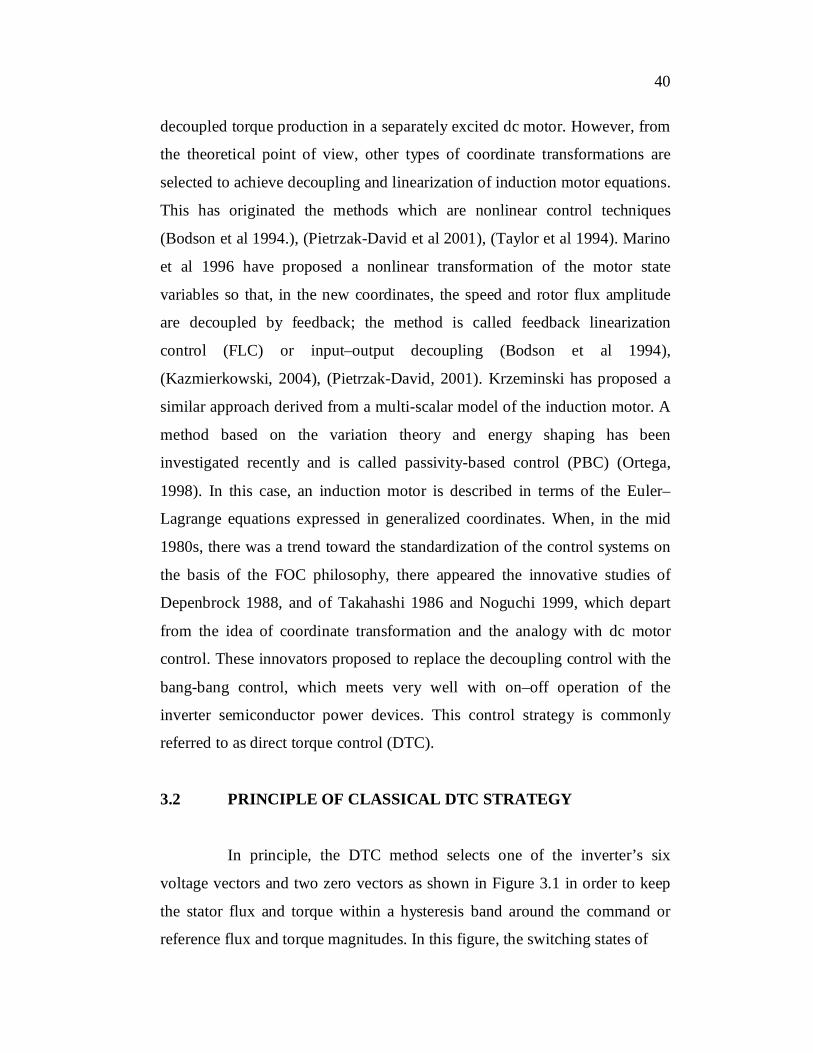
Table 3.1 Switching states of inverter
Voltage Vectors
Switching States
A B C
V0 0 0 0
V1 1 0 0
V2 1 1 0
V3 0 1 0
V4 0 1 1
V5 0 0 1
V6 1 0 1
V7 1 1 1
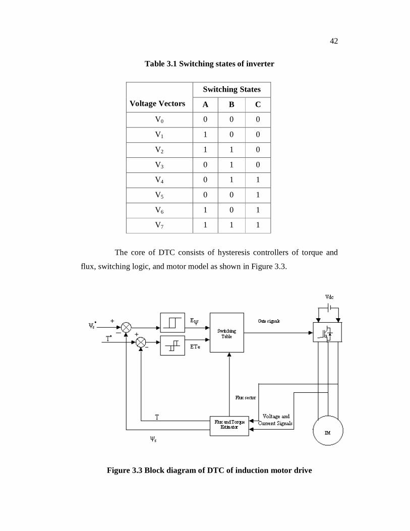
The core of DTC consists of hysteresis controllers of torque and
flux, switching logic, and motor model as shown in Figure 3.3.
Figure 3.3 Block diagram of DTC of induction motor drive

43
Figure 3.3 shows the basic schematic diagram of classical direct
torque control strategy of induction motor in which there are two different
loops corresponding to magnitudes of stator flux and torque provided. The
reference values of stator flux and torque are compared with the
corresponding actual values calculated by the motor model and the respective
errors are obtained. The resulting flux error is fed into the two level flux
hysteresis and torque error is fed into three level hysteresis controllers. The
outputs of torque and flux hysteresis controllers are combined together with
the position of stator flux and given as inputs to the switching state selection
table. The position of stator flux is divided into six different sectors. With
reference to the block diagram of DTC, the stator flux and torque errors tend
to be restricted within the hysteresis bands. The flux hysteresis band affects
basically the stator current distortion in terms lower order harmonics and
torque hysteresis band affects the switching frequency (Vas Peter, 1998). The
DTC requires the stator flux and torque estimations, which are performed by
means of two different phase currents and state of the inverter. However, flux
and torque estimations can also be performed using mechanical speed and two
stator phase currents. The switching logic defines the suitable voltage vector
based on torque and flux references. Table 3.2 shows the voltage vector
selection table. As described earlier, the flux controller is a two level
comparator while torque controller is a three level comparator.
The digitized output signals of the flux controller are defined as
1E for Hs * (3.1)
1E for Hs *
(3.2)

44
and those of the torque controller as
ETe=1 for eTe HTT * (3.3)
ETe= 0 for *TTe (3.4)
ETe= -1 for eTe HTT * (3.5)
where H is the flux tolerance band and
eTH is the torque tolerance band of
the hysteresis comparators. The digitized variables E , ETe and the stator flux
sector obtained from the angular position,
sd
sq
1tan , the appropriate
voltage vector is selected as shown in Table 3.2.
Table 3.2 Vector selection table
Sector
E ETe 1 2 3 4 5 6
↑
↑ V2 V3 V4 V5 V6 V1
0 V0 V0 V0 V0 V0 V0
↓ V6 V1 V2 V3 V4 V5
↓
↑ V3 V4 V5 V6 V1 V2
0 V0 V0 V0 V0 V0 V0
↓ V5 V6 V1 V2 V3 V4
3.3 STATOR FLUX AND TORQUE ESTIMATION
The direct torque control strategy does not require speed or rotor
position sensors. Stator flux and torque estimation based on the stator voltage
equations does not require speed or position information when stationary

45
coordinates are applied. Thus, from the state of the voltage source inverter
and having the instantaneous value of dc link voltage, phase voltage of the
motor is deduced. Once the voltage and current values are obtained, they are
transformed into d and q components by means of Park’s transformations.
Then the stator flux linkage in the final form is obtained as
dtRiv ssss (3.6)
The above equation is descretized as
ssss RivTs
zz
..1 1
1
(3.7)
The above equation is expressed in time domain as
11.1 kiRTkvTskk ssssss (3.8)
The d and q components of the above equation are
11.1 kiRTkvTskk sdsssdsdsd (3.9)
11.1 kiRTkvTskk sqsssqsqsq (3.10)
The stator voltage space vector components are derived from the
inverter internal switch settings. So, measurement of stator voltage is not
required. In practice, the calculation of d and q axes components of stator
voltage space phasor is done using dc link voltage value only. It should be
noted that a coordinate transformation is not required. However, the accuracy

46
of the estimation is limited due to the open loop integration that can lead to
large stator flux estimation errors.
3.4 METHODS OF DTC
In the classical DTC, there are several drawbacks. They are
summarized as follows:
(i) Sluggish or slow torque and flux response during start-up.
(ii) Large and small torque or flux errors are not distinguished
(iii) The same vectors are used during start-up, step changes and
steady state conditions.
In order to overcome the above mentioned drawbacks, the
following techniques are used:
(i) Modified switching table technique
(ii) Deadbeat control technique
(iii) Constant switching frequency technique
(iv) Intelligent control techniques
3.4.1 Modified switching table technique
Many modifications can be done in switching table aimed at
improving starting and overload conditions, very-low-speed operation, torque
ripple reduction, variable switching frequency functioning, and noise level
attenuation, (Kazmierkowski, 2004).

47
These are accomplished using the following methods
(i) Six sector table with variable zones (Category-I)
(ii) Twelve sector table (Category –II)
3.4.1.1 Six-sector table with variable zones (Category-I)
During starting and very-low-speed operation the basic switching
table -DTC scheme selects many times the zero voltage vectors resulting in
flux level reduction owing to the stator resistance drop. This drawback is
avoided by using either a dither signal (Kazmierkowski, 2004), (Noguchi,
1999) or a modified switching table in order to apply all the available voltage
vectors in appropriate sequence (Vas Peter, 1998). Table 3.3, shows the
comparison of operating zones of Classical DTC and Modified DTC and
look -up of table for this category is shown in Table 3.4.
Table 3.3 Comparison of operating zones of Classical DTC and
Modified DTC (Category-I)
Voltage Vectors Classical DTC DTC with changes of zones
(Category-I)
V1 +30 to -30 +0 to -60
V2 +90 to +30 +60 to 0
V3 +150 to +90 +120 to +60
V4 -150 to +150 +180 to +120
V5 -90 to -150 -120 to -180
V6 -30 to -90 -60 to -120

48
Table 3.4 Look-up Table for Category-I
Flux Torque S1 S2 S3 S4 S5 S6
Increase↑
Increase↑ V2 V3 V4 V5 V6 V1
Zero V0 V7 V0 V7 V0 V7
Decrease↓ V1 V2 V3 V4 V5 V6
Decrease↓
Increase↑ V4 V5 V6 V1 V2 V3
Zero V7 V0 V7 V0 V7 V0
Decrease↓ V5 V6 V1 V2 V3 V4
3.4.1.2 Twelve-sector table with variable zones (Category-II)
Stator flux locus is divided into twelve sectors instead of six sectors
in classical DTC. In this method all six active state voltage vectors are used
per sector. Unlike classical DTC, the alternative procedure is introduced. That
is, instead of just torque increase and torque decrease, small or slight increase
and decrease in torque are also introduced. Since, tangential voltage vector
component is very small, the small variation in torque should also be taken
into account. The look up table for this category is shown in Table 3.5.

49
Table 3.5 Look-up Table for Category-II
Flux Torque S1 S2 S3 S4 S5 S6 S7 S8 S9 S10 S11 S12
Increase
Increase V2 V3 V3 V4 V4 V5 V5 V6 V6 V1 V1 V2 Slightly Increase
V2* V2 V3
* V3 V4* V4 V5
* V5 V6* V6 V1
* V1
Slightly Decrease
V1 V1* V2 V2
* V3 V3* V4 V4
* V5 V5* V6 V6
*
Decrease V6 V1 V1 V2 V2 V3 V3 V4 V4 V5 V5 V6
Decrease
Increase V3 V4 V4 V5 V5 V6 V6 V1 V1 V2 V2 V3 Slightly Increase
V4 V4* V5 V5
* V6 V6* V1 V1
* V2 V2* V3 V3
*
Slightly Decrease
V7 V5 V0 V6 V7 V1 V0 V2 V7 V3 V0 V4
Decrease V5 V6 V6 V1 V1 V2 V2 V3 V3 V4 V4 V5
3.4.2 Deadbeat Control
The main idea behind a dead-beat DTC scheme is to force torque
and stator flux magnitude to achieve their reference values in one sampling
period by synthesizing a suitable stator voltage vector applied by Space
Vector Modulation. In this approach (Barbara, Robert, 2003), (Lee et al 2002)
the changes of torque and flux over one sampling period are at first predicted
from the motor equations, and then a quadratic equation is solved to obtain
the command value of stator voltage vector in stationary coordinates (Yang,
2002).
3.4.3 Constant Switching Frequency Approach
The inverter frequency is maintained constant and greater than the
sampling frequency, which will reduce the torque and flux ripple
dramatically. Different space vector modulation techniques are used in this
50
approach and no dead-beat control is applied (Jun Koo Kang, Seung Ki Sul,
1999), (Idris, Yatim, 2000).
3.4.4 Intelligent Methods (or) Artificial Intelligence Methods of DTC
Artificial Intelligence (AI) techniques are recently finding
widespread applications in science and engineering. AI is basically
embedding human intelligence in a machine so that a machine can think
intelligently like a human being. The AI computing techniques are classified
as (i) Hard computing (ii) Soft computing techniques. In this section,
principle and application of soft computing techniques such as Artificial
Neural Networks, Fuzzy Logic and Genetic Algorithms into DTC of
induction motor drive have been discussed.
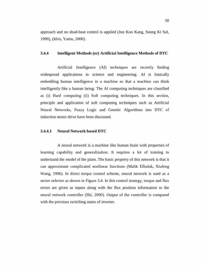
3.4.4.1 Neural Network based DTC
A neural network is a machine like human brain with properties of
learning capability and generalization. It requires a lot of training to
understand the model of the plant. The basic property of this network is that it
can approximate complicated nonlinear functions (Malik Elbuluk, Xiufeng
Wang, 1996). In direct torque control scheme, neural network is used as a
sector selector as shown in Figure 3.4. In this control strategy, torque and flux
errors are given as inputs along with the flux position information to the
neural network controller (Shi, 2000). Output of the controller is compared
with the previous switching states of inverter.

51
Artificial Neural Network (ANN) offers the following advantages
over other conventional DTC schemes for induction motors,
i) Reduction of the complexity of the controller;
ii) Reduction of the effects of motor parameter variations,
particularly in the stator-flux estimation;
iii) Improvement of controller time response, i.e., the ANN
controller uses only parallel processing of sums, products by
constant gains, and a set of well known non-linear functions
to reduce computation time.
iv) Improvement of drive robustness – ANN’s are fault tolerant
and can extract useful information from noisy signals
-
s
Te
IM Flux and Torque
Estimator Motor signals
Switching Table
Error
ANN
Flux sector
+ + +
-
- -
V1 V2 V3
+
+
-
Te*
s*
ETe
s
Vdc + -
Figure 3.4 Schematic of DTC using Neural-Network controller
3.4.4.1.1 Principles of Artificial Neural Networks
Feed forward artificial neural networks are universal approximators
of nonlinear functions (Malik Elbuluk, 1996). As such, the ANNs use a dense
interconnection of neurons that correspond to computing nodes. Each node

52
performs the multiplication of its input signals by constant weights, sums up
the results, maps the sum to a nonlinear function and the result is then
transferred to its output. The structure of neuron is shown in Figure 3.5 and
the mathematical model of a neuron is given by
N
iii bxy
1 (3.11)
where, Ni xxxx ,,, 21 are inputs from the previous layer neurons
Ni ,,, 21 are the corresponding weights, and ‘b’ is the bias of
the neuron. For a logarithmic sigmoidal activation function, the output is
given by
N
iii bx
e
y11
1
(3.12)
Neuron j
+1
th j
i
1
n j
threshold
m nj j
m 1j
x 1
x nj
x i
layer n-1
layer n
y jn 1
1+ ec jn y j
n
n
nm ij
n
n
n
n-1
n-1
n-1
i=1
n j+ th jm
ijn
ixn-1 jx n
Figure 3.5 Structure of Neuron
A feed forward neural network is organized in layers: an input
layer, one or more hidden layers, and an output layer. No computation is
performed in the input layer and the signals are directly supplied to the first
hidden layer through input layer. Hidden and output neurons generally have a

53
sigmoidal activation function. The knowledge in an ANN is acquired through
a learning algorithm, which performs the adaptation of weights of the network
iteratively until the error between the target vectors and output of network
falls below a certain error goal. The most popular learning algorithm for
multi-layer networks is the back propagation algorithm, which consists of a
forward and backward action. In the first, the signals are propagated through
the network layer by layer. An output vector is thus generated and subtracted
from the desired output vector. The resultant error vector is propagated
backward in the network and serves to adjust the weights in order to minimize
the output error. The back propagation training algorithm and its variants are
implemented by many general – purpose software packages such as the
neural-network toolbox in MATLAB (Howard Demutth, 1998), (William,
2001) and the neural-network development systems described by Bose (Bose,
1996). The time required to train an ANN depends on the size of the training
data set and training algorithm. An improved version of back propagation
algorithm with adaptive learning rate is proposed which permits a reduction
of the number of iterations. Figure 3.6 shows the proposed neural network for
DTC scheme in which, input, output and hidden layers are shown. The error
signals and stator flux angle are given to input layer. Switching state
information is taken from the output layer. Figure 3.7 shows the flowchart of
proposed neural network controller of DTC algorithm.
In p u t L ayer H id d e n lay er O u tp u t L ay er
E T e
E ψ e
θ
t1
t2
t3
Figure 3.6 Structure of Neural network proposed for DTC scheme

54
No
Start
Test the induction motor drive system with neural network controller and fix the neural
network input and output data
Calculate torque and flux errors
Is selection of switching state
acceptable?
Add the position of stator flux
Based on neural network input calculate expected neural network output
Add neural network input and calculate expected neural
network output to train data
Train the Neural network controller with new data
End
Yes
Figure 3.7 Flowchart for Neural Network based DTC of induction motor

55
3.4.4.2 Fuzzy Logic based DTC
This technique is based on applying switching state to the inverter
and the selected active state to achieve the torque and flux references values.
A null state is selected for the remaining switching period, which won't
change both the torque and the flux. Therefore, the switching state has to be
determined based on the values of torque error, flux error and stator flux
angle. Exact value of stator flux angle “θ” determines the position of stator
flux. The schematic of fuzzy logic direct torque control scheme for induction
motor drive is shown in Figure 3.8. Flowchart of the fuzzy control of DTC is
shown in Figure 3.9.
s
Te
Motor signals
Vdc + -
IM
Flux and Torque Estimator
Switching Table
Fuzzy Controller
Flux sector
+
-
Te*
- + s
*
ETe
s
Fuzzy
Fuzzy
Fuzzy
Figure 3.8 Schematic of fuzzy logic DTC

56
Start
Inputs – Torque value, flux value and Position of stator flux
Fuzzification
Decision Making Logic- Big or small
Defuzzification
Entire Control Process
Outputs – Torque value, flux value and Position of stator flux
If Output is equal
to Desired Value
Desired Voltage Vector from the inverter
Yes
No
Figure 3.9 Flowchart for Fuzzy Logic based DTC

57
The fuzzy output of torque, flux errors and stator flux angle are
given as input variables to fuzzy controller and output variable obtained from
the fuzzy controller is switching state of the inverter which is a crisp value
(Mir et al 1994), (Yang Xia et al 1997). The membership functions of input
variables such as torque error, stator flux error and stator flux angle are shown
in Figure 3.10 (a), (b) and (c) respectively.
(a)
(b)
(c)
Figure 3.10 Membership distributions for input variables (a) Torque
Error (b) Flux Error and (c) Stator Flux angle

58
3.4.4.2.1 Fuzzy Rules for Direct Torque Control Scheme
The fuzzy system comprises 12 groups of rules and each group
contains 15 rules. Each group represents the respective stator flux angle θ.
The rules are shown in Table 3.6 for stator flux angle θ1, θ2 and θ3. For every
combination of inputs and outputs, one rule is applied. Totally, there are
twelve-stator flux angles from 1 to 12 and 180 rules are formed. With the
help of them, corresponding switching state of the inverter is selected.
Table 3.6 Fuzzy Rules Developed for Direct Torque Control Technique
1 2 3
Eψ
ETe P Z N P Z N P Z N
PL V1 V2 V2 V2 V2 V3 V2 V3 V3
PS V2 V2 V3 V2 V3 V3 V3 V3 V4
ZE V0 V0 V0 V0 V0 V0 V0 V0 V0
NL V6 V0 V4 V6 V0 V5 V1 V0 V5
NS V6 V5 V5 V6 V6 V5 V1 V6 V6
From the rules, fuzzy inference equations are given as
),),(min( iteiii CEBEA (3.13)
nNinNi i ,min' (3.14)
180
1
'maxi
nNinN (3.15)

59
3.4.4.3 Adaptive Neuro-fuzzy based direct torque control method
Adaptive Neuro-fuzzy controller is a hybrid intelligent controller,
since it combines two intelligent systems, viz., neural networks and fuzzy
systems. The basic idea of combining is to design an architecture that uses
(i) The learning ability of a neural network to optimize its
parameters and
(ii) Fuzzy system to represent knowledge in an interpretable
manner
The drawbacks in both of the individual approaches, viz., the black
box behavior of neural networks and the problem in finding suitable
membership values for fuzzy systems can thus be avoided. Human expert
knowledge is used to build the initial structure of neuro-fuzzy controller. The
Adaptive Neuro-fuzzy Inference System (ANFIS) structure (Janj, Sun 1995)
is one of the advanced methods to combine fuzzy logic and artificial neural
networks. A neuro-fuzzy inference system contains rule base and data
(knowledge) base, fuzzification and defuzzification unit. The proposed
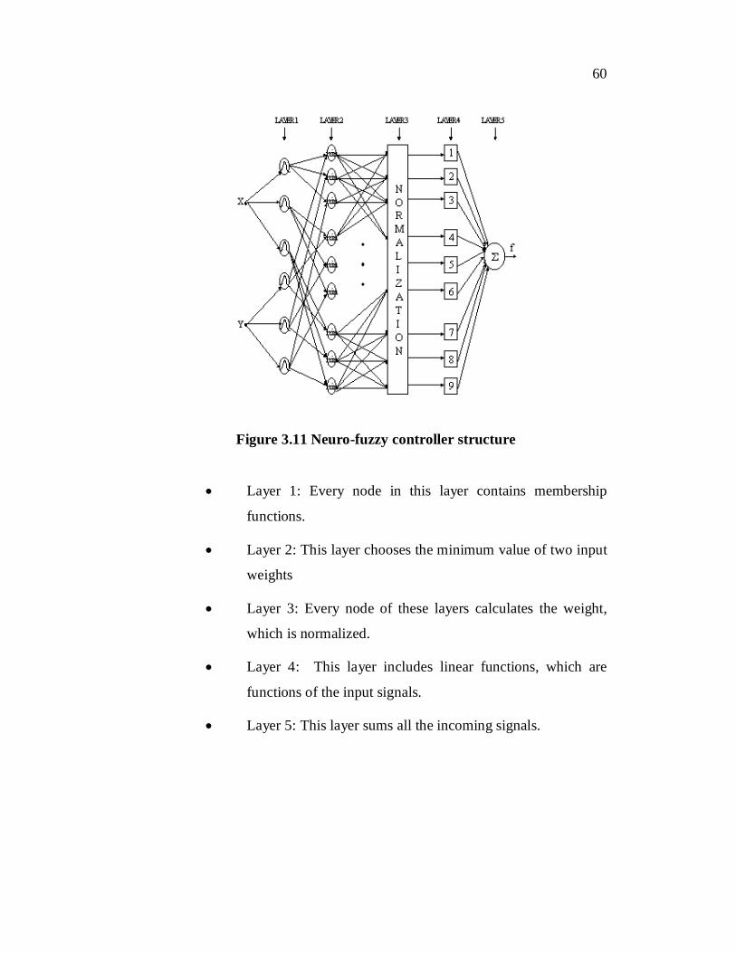
structure shown in Figure 3.11 contains five network layers (Grabowski et al
2000) as follows:
60
Figure 3.11 Neuro-fuzzy controller structure
Layer 1: Every node in this layer contains membership
functions.
Layer 2: This layer chooses the minimum value of two input
weights
Layer 3: Every node of these layers calculates the weight,
which is normalized.
Layer 4: This layer includes linear functions, which are
functions of the input signals.
Layer 5: This layer sums all the incoming signals.

61
In an ANFIS, a fuzzy inference system is designed systematically
using the neural network design method. Usually Sugeno method of
implication is used in an ANFIS (Bose, 2002). A fuzzy inference process
consists of the following five steps:
Fuzzification of input variables
Application of fuzzy operator in the antecedent part of the
rule
Implication from the antecedent to the consequent
Aggregation of consequents
Defuzzzification
In Figure 3.11, Layer 1 corresponds to fuzzification of input
variables and layer 2 corresponds to the application of fuzzy operator and the
layer 3 does the implication. Layer 4 and layer 5 both together aggregate the
rules. The output ‘f’ is then defuzzified to produce crisp output. During the
training of ANFIS, both the weights and membership functions are modified
using the back-propagation training algorithm.
The flux error Eψs and torque error ETe multiplied by suitable
weights are delivered to three membership functions in both inputs. The
membership functions for flux error (Eψs) and torque error (ETe) are chosen
to be bell-shaped and is shown in Figure 3.12.

62
Figure 3.12 Bell shaped membership functions for flux and torque errors
The block diagram of Direct-Torque Neuro-Fuzzy Control
(DTNFC) scheme is shown in Figure 3.13. The error signals, Eψs and ETe are
delivered to the Neuro-Fuzzy (NF) controller, which uses the information on
the position (θ) of the actual stator flux vector, to generate the signal that
selects the switching states and hence generates the Sa, Sb, Sc pulses to control
the switches in the inverter.

63
s
Te Motor signals
Vdc + -
IM
Flux and Torque Estimator
Switching Table
ANFIS Controller
Flux sector
+
- Te
*
- + s
*
ETe
s
Figure 3.13 Block diagram of Adaptive direct torque neuro-fuzzy
control method
3.4.4.4 Genetic algorithm based Direct Torque Control method
Genetic algorithms are stochastic global search algorithms. They
mimic processes observed in natural evolution and use a vocabulary borrowed
from the natural genetic. A GA considers individuals in a population quite
often called strings or chromosomes and must have the following
components:
i) A genetic representation for potential solution encoded as
strings or chromosomes.
ii) A way to create an initial population of potential solutions
iii) An evaluation function for rating solutions in terms of their
fitness
iv) Genetic operator that alter the composition of children

64
v) Values for various parameters that the genetic algorithm
uses (population size, probabilities of applying genetic
operators, etc.).
Given these five components, a genetic algorithm is constructed as follows:
i) Initialize a population of chromosomes.
ii) Evaluate each chromosome in the population.
iii) Select chromosomes in the population as parent
chromosomes to reproduce.
iv) Apply the genetic operators to the parent chromosomes to
produce children.
v) Evaluate the new chromosomes and insert them into the
population.
vi) If the termination condition is satisfied, stop and return the
best chromosome. If not go to step (iii).
For executing genetic algorithm to train the neural networks,
certain procedures were followed. Figure 3.16 shows the flowchart to execute
a genetic algorithm. It gives an algorithm to select the best chromosome from
the total population of chromosomes. To select best chromosome, parent
selection is important. Steps for parent selection are as summarized as
follows:
i) Selection of parents for reproduction is stochastic.
ii) Selection of parents with higher fitness value.
iii) Roulette wheel technique for parent selection. A roulette
wheel shown in Figure 3.14 has slots, which are sized
according to the fitness of each chromosome.
iv) Selection process is to spin the roulette wheel.

65
In Figure 3.14, 54321 ,,,, fffff are fitness of chromosomes 1, 2, 3, 4
and 5, respectively. If total number of chromosomes is 50, population size is
also 50. Therefore,
50ff pop Fitness of 50th chromosome (3.16)
Total fitness is given by, F= Sum of the fitness of the population
pop
jjevalF
1 (3.17)
Probability function for each chromosome is
popiFevalp ii ,,3,2,1,/ . Accumulative probability function for each
chromosome is
popipqi
jii ,,3,2,1,
1
(3.18)
f1f 2
f 3
f 4
f 5
f pop
Figure 3.14 Roulette Wheel

66
3.4.4.4.1 Neural Networks Trained By Genetic Algorithms
In neural networks, genetic algorithms are used to determine the
weights and threshold values. Figure 3.15 shows the structure of neural
networks trained using GA. The respective error vectors between the state
selector of conventional DTC and the neural networks outputs are 321 ,, eee . To
achieve minimum value of performance index, the groups of threshold values
and weights have to be determined.
t 1
t 2
t 3
r2
r1
+1 +1threshold threshold
u 1
u 2
e1
e 2
e 3
m 112
m 111
m 532m
351
th 11
12th
layer 1 layer 2
+
+
+
-
-
-
u 3
layer 3
r3
Figure 3.15 Structure of neural networks trained using GA
Performance index E (W) are given by:
jejeWEN
j
T 12
1 (3.19)
where: TT eeee 321 = error vectors
Symmetric positive definite matrix
N = Sample size
Implementation of the genetic algorithm described in this research
has three stages.

67
i) Fitness evaluation
Evaluate the individual fitness of a certain proportion of the
population
ii) Selector
Selector selects the best-ranking individuals to reproduce
iii) Breeding
The breeding function generally works by taking portions of each
solution and linking them together into a new one. Solutions are often
represented as strings, so generally, a breeding function will take fragments of
random lengths from each string and join them together to form a new string.
The genetic operators used in this work are quite different from the
classical ones used in (Malik Elbuluk, 1996).
The main differences between the proposed work and existing work
are described as follows:
(i) The real valued space are dealt, where a solution is coded as
a vector with floating point type components
(ii) Some genetic operators are non-uniform, that is, their action
depends on the age of the population.
The contents of the algorithm are listed below:

68
3.4.4.4.2 Chromosome Encoding
Let the total number of thresholds and weights of the neural
network shown in Figure 3.15 be packed in the n-dimensional vector W,
3821135
115
15
251
211
21 wwwmmthmmthW (3.20)
Here, W is the weights vector as a chromosome (individual). In
other words, each chromosome vector is coded as a vector of floating point
numbers of the same length. Each element is initially selected to be within the
desired domain.
3.4.4.4.3 Evaluation function
The evaluation function for chromosomes ‘w’ is
)(1
100)(WE
Weval
(3.21)
where, the chromosome vector w is a real weights vector, and E(w) is defined
by equation (3.19). The evaluation function is used to rate a chromosome in
terms of their “fitness”. Both binary and floating point encoding are used as
genetic operators to train the neural networks in DTC technique. The binary
operators are one point crossover, two points crossover and bit mutation. The
operators used for floating point encoding are different from classical ones.
They work in a real valued space. However, because of intuitive similarities,
they are divided into the standard classes of mutation and crossover groups.
Mutation groups used in this research are Uniform mutation (UM), Non-
Uniform Mutation (NUM) and Non- Uniform Arithmetical Mutation
(NUAM). Crossover groups are Two-Points Crossover (TPC) and Two-Points
Arithmetical Crossover (TPAC).

69
Initialize a population of chromosomes
Evaluate each chromosome in the population
Select chromosomes with higher evaluation in
population as potential parents
Evaluate the new chromosomes and insert them into new
population
Delete member of the population to make room for the new
chromosomes
Apply the genetic operators to the parent chromosome to produce
children
Stop
If Satisfied?
Return the best chromosome
Start
Yes
No
Figure 3.16 Flowchart for execution of a Genetic Algorithm
70
3.5 SIMULATION RESULTS AND DISCUSSIONS
A 3-phase 1 HP induction motor is used for simulation. The
parameters of the machine are determined experimentally and are given in the
Appendix -1. For the simulation of the viable torque control schemes, Voltage
source inverter (VSI) is employed. The simulations are carried out using
MATLAB / SIMULINK (William, 2001). Results obtained for viable torque
and flux control techniques such as conventional DTC, DTC using neural
networks, DTC using neural networks trained with genetic algorithm and
DTC using fuzzy logic have been discussed. Switching frequency of the
inverter taken for simulation was 10 kHz. Therefore, the sampling time taken
for simulation was 100μsec. Torque and flux reference values taken were
1 Nm and 1 web when torque and flux hysteresis values are 0.5 Nm and
0.02 web respectively. An index error has been used to quantify the error in
both the stator flux and torque responses. This index is the integral of the
square error (IE2), which is computed by means of the square error instead of
just the error. Errors obtained in control schemes have been compared with
each other. The error comparison is shown in Table 3.8.
3.5.1 Conventional Direct Torque Control Strategy
SIMULINK diagram of conventional DTC is shown in Figure 3.17.
This SIMULINK schematic consists of torque hysteresis controller, flux
hysteresis controller, sector selector, optimal switching logic, PWM inverter
and Motor model modules. Each module consists of its own subsystems.

71
Figure 3.17 SIMULINK Diagram of Conventional Direct Torque
Controller
Figure 3.18 shows the speed response of induction motor using
conventional DTC strategy. Figure 3.19 shows the position of stator flux.
Figure 3.20 shows the stator current of induction motor at the application of
conventional DTC strategy. At the application of conventional DTC strategy,
stator flux linkages in stationary frames of induction motor are shown in
Figure 3.21. The components of stator flux linkages in stationary reference
frame are sinusoidal and 90º phase displacement to each other. Locus of
stator flux is shown in Figure 3.22 and it is noticed that flux follows a circular
shape. Figure 3.23 shows the sector selector and it is used to identify the
sector in which stator flux positioned. The value of the sector steps up
periodically from zero to six and the duration of each step coincides with a
period of the each switching time. The sum of each switching time is equal to
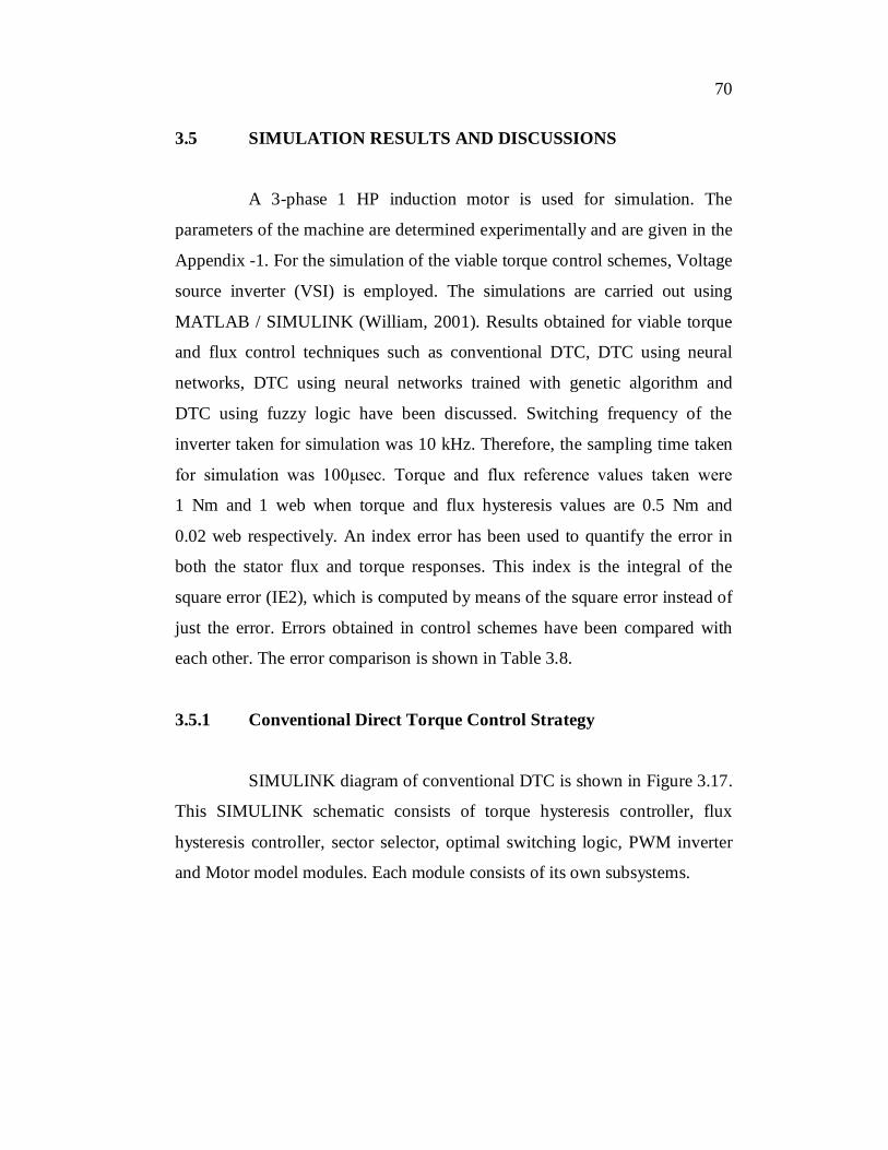
the total switching time at any point of time. Figure 3.24 shows the sector
selector and it is used to identify the sector when flux reversal happened.

72
Figure 3.18 Speed Response in Conventional DTC
0 0 . 0 5 0 . 1 0 . 1 5 0 . 2 0 . 2 5 0 . 3 0 . 3 5 0 . 4 0 . 4 5 0 . 50
0 . 1
0 . 2
0 . 3
0 . 4
0 . 5
0 . 6
0 . 7
0 . 8
0 . 9
1P o s it io n o f s t at o r f lu x
s (
pu)
t im e ( sec )
Figure 3.19 Position of stator flux

73
Figure 3.20 Stator currents of induction motor using conventional
Direct Torque controller
Figure 3.21 Stator flux linkages in stationary frames in induction motor
using conventional Direct Torque controller
Phase A
Phase B Phase C
d-flux q-flux

74
Figure 3.22 Locus of Stator Flux in Conventional DTC
Figure 3.23 Sector Identification
75
Figure 3.24 Sector Identification with field reversal
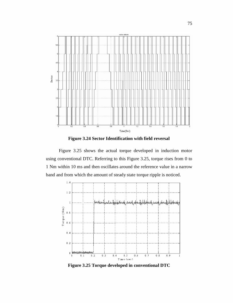
Figure 3.25 shows the actual torque developed in induction motor
using conventional DTC. Referring to this Figure 3.25, torque rises from 0 to
1 Nm within 10 ms and then oscillates around the reference value in a narrow
band and from which the amount of steady state torque ripple is noticed.
Figure 3.25 Torque developed in conventional DTC

76
3.5.2 Neural Network based Direct Torque Control Strategy
The neural network is trained using the MATLAB neural-networks
toolbox. This network consists of a three layer neural –network with three
input nodes connected to five log sigmoid neurons and three pure output
nodes connected to five log sigmoid neurons. The training strategy consists
the parallel recursive error prediction was chosen as a learning technique for
simulation purposes to update the weights of the neural network. The
algorithm was chosen because of its learning speed, robustness and high
learning capability. This algorithm is so powerful when complicated and
nonlinear functions are to be learned by the neural network. The neural
network structure mentioned previously was simulated using this algorithm
and using the hyperbolic tangent function
cx
cx
eecxxS
11
21tanh (3.22)
as the nonlinearity in the transfer functions of the hidden and output layers.
The parameter ‘c’ was fixed to one for all the cases. Small values of ‘c’ are
found to give larger weights and vice versa.
Simulation results were determined using an electromagnetic torque
and stator flux commands of 1 Nm and 1.0 Weber respectively. The switching
frequency of the inverter used by the simulations was 10 kHz. The neural
network frequency was chosen to give the system enough time to stabilize its
output. The data used to train the neural network have been determined by
direct simulation of DTC using a sampling frequency of 100 Hz.

77
Figure 3.26 shows the stator current of induction motor at the
application of neural network concept into direct torque control strategy.
Figure 3.27 shows the torque developed by the application of this strategy.
Figure 3.26 Stator three phase currents of induction motor using neural
network based Direct Torque control scheme
Figure 3.27 Torque developed using neural network based Direct Torque
control scheme
Phase A Phase B Phase C

78
3.5.3 Genetic Algorithm based Direct Torque Control Strategy
Neural network trained with genetic algorithm is implemented in
such a way that the total number of thresholds and weights of the neural
network be packed in n - dimensional vector ‘w’ as given in equation (3.23).
135
115
15
251
211
21 mmthmmthw (3.23)
where, th = threshold vector
m= weight vector
and n=38;
To represent the values of weights w, binary encoding or floating
point encoding is used as a chromosome. Genetic operators used for binary
representation are one point crossover, two-point crossover and bit mutation
and for floating point representation are two point arithmetical crossover,
uniform mutation, non-uniform mutation and non- uniform arithmetical
mutation. Table 3.7 shows the parameters used for simulation:
Table 3.7 Parameters used for Genetic Algorithm based DTC
Parameters used Binary
representation Floating point representation
Number of chromosomes 30 100
Crossover probability 0.8 0.9
Mutation probability 0.005 0.008
In binary encoding algorithm, Lower number of chromosomes was
used than floating point encoding algorithm. The performance of the system is
affected if number of chromosomes reduced. To improve the performance and

79
to overcome this drawback, the best member of each generation must be
copied into the succeeding generation. Crossover probability is chosen from
0.5 to 0.9. Convergence rate becomes slower with the higher crossover
probability values. Convergence rate should be in high bias level. Mutation
rate taken for simulation will make the convergence faster. In floating point-
encoding algorithm, non-uniform mutation and non-uniform arithmetic
mutation operators were introduced to prevent premature convergence. Fine
tuning capabilities of genetic algorithm were achieved by using these
operators and performance of the algorithm was also improved.
Figures 3.28 and 3.29 show the stator currents and Figures 3.30 and
3.31 show the actual torque developed in induction motor by the application
of Genetic Algorithm based DTC in which Figure 3.28 and 3.30 for binary
coding representation. Figures 3.29 and 3.31 represent the floating point
coding representations.
Figure 3.28 Stator three phase currents of induction motor using
Genetic Algorithm based Direct Torque control scheme
(Binary Coding)
Phase A Phase B Phase C

80
Figure 3.29 Stator three phase currents of induction motor using
Genetic Algorithm based Direct Torque control scheme
(Floating point Coding)
Figure 3.30 Torque developed using Direct Torque Neuro controller
trained by genetic algorithm (Binary coding representation)
Phase A Phase B Phase C

81
Figure 3.31 Torque developed using Direct Torque Neuro controller
trained by genetic algorithm (Floating Point coding
representation)
3.5.4 Fuzzy Logic based Direct Torque Control Strategy
Direct torque control of induction motor using fuzzy logic was also
simulated using the MATLAB / SIMULINK package. Fuzzy rules are formed
for twelve flux angle positions and membership functions were formed.
Simulations include all the possible 180 rules are carried out. Figure 3.32
shows the SIMULINK diagram of the direct torque fuzzy logic controller.
Figure 3.33 is the torque developed by fuzzy controller.

82
Figure 3.32 SIMULINK Diagram of Direct Torque Fuzzy Controller
Figure 3.33 Torque developed using Direct Torque fuzzy controller

83
3.5.5 Adaptive Neuro Fuzzy Inference System (ANFIS) based Direct
Torque Control Strategy
Figure 3.34 shows the SIMULINK diagram of ANFIS, which has
been used to select the appropriate voltage vectors from the information of
torque error, flux error and position of stator flux. Simulation of ANFIS based
direct torque controller is done in two stages
(i) A set of membership functions is chosen.
(ii) The input- output training data is used by ANFIS. It starts
making a clustering study of the data to obtain a concise and
significant representation of the system’s behavior. It is
important to note that the system has a good modeling if the
training set has enough representative, i.e., it has a good data
distribution to make possible to interpolate all necessary
values of the system. The clustering technique used was the
fuzzy c-means. After setting the number of clusters that are
estimated to compose the data, the cluster’s centers are
searched in an iterative way based on minimizing an
objective function.
Figure 3.34 Schematic of ANFIS based direct torque controller

84
Figure 3.35 shows the torque developed in induction motor using
ANFIS based direct torque control strategy.
Figure 3.35 Torque developed using Direct Torque neuro fuzzy controller
From the graphs of torque developed, it is cleared that the different
DTC strategies have a very good torque response that is the torque rises very
fast and reaches steady state value quickly.
From the Table 3.8, it is realized that the index errors for flux and
torque have been calculated for the different values of torque and speed in
terms of their respective nominal values.

85
Table 3.8 Errors obtained in various control strategies
Index Error (EI) Classical DTC DTC_NN DTC_NN_GA DTC_ Fuzzy
T=a*Tn =b*n Flux Torque Flux Torque Flux Torque Flux Torque
a = 100% b = 10% 2.53 e-3 0.189 2.2 e-3 0.165 1.97 e-3 0.156 2.74e-3 0.169
a = 50% b = 50% 2.57 e-3 0.068 0.53 e-3 0.025 0.68 e-3 0.023 0.88 e-3 0.033
a = 10% b = 10% 7.46 e-3 0.0367 1.58 e-3 0.0014 5.68 e-3 0.0015 0.14 e-3 0.00135
a = 100% b= 100% 2.46 e-3 0.297 2.1 e-3 0.263 2.33 e-3 0.31 2.55 e-3 0.251

86
3.6 CONCLUSION
In this chapter, principle and methods of torque control schemes
such as Neural network based direct torque control, Genetic algorithm based
direct torque control, Fuzzy logic based direct torque control and Neuro
Fuzzy based direct torque control have been evaluated for induction motor
drive and which have been compared with the conventional direct torque
control technique. Each strategy has individual advantages and limitations
are given in Table 3.9.

87
Table 3.9 Comparison of DTC Techniques
Sl. No.
Control Strategies Advantages Limitations
1. DTC using Neural Network
1. Many training methods such as Back propagation algorithm, parallel recursive method, Kalman filter method and adaptive neuron model methods are available.
2. The results obtained are very close to conventional DTC.
1. Training time required is more. 2. Affected by parameters of the machine changes.
2. DTC using Genetic Algorithm (Binary Representation)
1. It is not highly sensitive to parameter of the machine changes. 2. Gives precise results.
1. Accuracy is affected when domain size increases. 2. Difficult to design for handling non-trivial constraints.
3. DTC using Genetic Algorithm (Floating point Representation)
1. It is also used to improve the performance on numerical problems. 2. Capable of representing quite large domains. 3. In this representation, it is easier to design special tools for handling non-trivial constraints.
1. In floating point representation, the genetic operators needs careful designing to preserve the constraint.
4. DTC using Fuzzy Logic
1. Fuzzy logic does the resistance compensation in DTC at low speed region. 2. Provides more accuracy
1. Many rules are required to provide accuracy. 2. Computational time required is high.
5. DTC using Adaptive Neuro Fuzzy algorithm
1. Combines the advantages of both the neural network and fuzzy logic 2. Good response
1. Computational time required is high.