chapter 3 spectral -temporal variations of aod in the...
TRANSCRIPT

34
Chapter 3 Spectral -Temporal variations of AOD in the context of meteorological parameters at Kannur
Aerosols offer scattering centers to the incoming solar radiation in the
atmosphere. Measurements of AOD provide the simplest and effective method to
analyze the aerosol properties both qualitatively and quantitatively. The scattered
intensities of various wavelengths depend on the size of the particles, and hence the
spectral variations of AOD can effectively be used for estimating the size distribution of
particles and their seasonal variations (Ranjan et al., 2007). Currently, MICROTOPS II
offers a prominent sun photometer for direct retrieval of seasonal and annual variabilities
of AOD.
In this chapter, the diurnal and seasonal variations of AOD measured by using a
MICROTOPS II at five discrete wavelengths over Kannur during a period of three years
from November 2009 to May 2012 are discussed. The relative domination of fine mode
aerosols over coarse mode aerosols is analyzed using Angstrom power law. The
Angstrom parameters (α and β) are the simplest indicators commonly used to classify the
relative abundance of fine to coarse mode particles and turbidity of the atmosphere
(Angstrom, 1964; Iqbal, 1983). The Angstrom parameters derived from both the liner
and polynomial fit are analysed. This investigation reveals that AODs are strongly
influenced by seasonal variations at this site. One of the significant features of
observation is that AODs are quite higher in April (~0.401 at 440nm) and relatively low
during November-December (~0.208 at 440nm). Thus this observation throws light to

35
the mounting concentrations of particulate matter present in the atmosphere during the
co-ordination of fireworks associated with Vishu and temple festivals that are usually
celebrated in the month of April, which causes a dramatic rise in AOD. Moreover, the
AOD values measured at different geographical locations under the field campaign are
compared with those observed at Kannur.
3.1 Instrument used for the study
Spectral AOD measurements were made using a MICROTOPS II of Solar Light
Company, USA, and the details of the instrument are available in research publications
(Morys et al., 2001 ; Ichoku et al., 2002). It is a five channel hand held sun photometer to
measure the instantaneous aerosol optical depth from individual measurements of direct
solar flux, using a set of internal calibration constants. Internal baffles are integrated into
the device to eliminate internal reflections.
The MICROTOPS II used in this study has optical filters transmitting the
radiation centered at wavelengths of about 340, 440, 675, 870 and 1020 nm with a full
width at half maximum (FWHM): ±2 – 10 nm. Therefore, investigations of the spectral
variation of aerosol attenuation within the near UV, visible and near infrared regions
could be analyzed and are highly informative (Adeyewa and Balogun, 2003; Ranjan et
al., 2007). A sun target and pointing assembly is permanently attached to the optical
block. As the image of the sun is centered in the bull’s-eye of the sun target, all optical
channels are oriented directly at the solar disc. A small amount of circumsolar radiation
is also captured, but it makes little contribution to the signal. Radiation captured by the
collimator and band pass filters, produce electrical current that are proportional to the
radiant power. These signals are first amplified and then converted to a digital signal by
a high resolution A/D converter and are processed in series with high speed. AOD is

36
retrieved in MICROTOPS by validating the Beer Lambert’s law. The optical depth
resulting from Rayleigh scattering is always subtracted from the total optical depth to
obtain AOD. (Optical depth from other processes, such as O3 and NO2 absorption is
ignored in MICROTOPS II). AOD at a particular wavelength is computed as
AODλ = [ ln(V0λ) – ln (Vλ *SDCORR) / m] – τRλ * (P/P0) (1)
where lnV0λ is the AOD calibration constant, Vλ is the signal voltage in mV, SDCORR is
the mean earth-sun distance correction, m is the air mass and τRλ is the correction for the
Rayleigh’s scattering. P is the atmospheric pressure at the observation site and P0 that at
the ground level. MICROTOPS II stores two sets of calibration constants: the factory
calibrations (FC) and user calibrations (UC). The FC is programmed into the instrument
during the calibration process and any modifications are restricted for the user. The UC
are initially set to equal FC but can be individually modified from the instrument's
keypad. Values for AOD and irradiance are not stored in memory at the time of
measurement. Instead, the raw data in millivolt (mV) is stored and the AOD and
irradiance values are calculated based on the recorded voltage and user calibration
constant and the results are displayed. For a reliable performance the instrument must be
calibrated periodically; either by Langley technique or by inter-comparison with a newly
calibrated sun photometer.
3.2 Theoretical background
The chemical composition of aerosols and their size distribution are affected by
various transformation processes. But the resultant spectral aerosol extinction coefficient
is governed by a simple analytical relation (Angstrom, 1929)
extk b αλ−= (2)

37
where α is called the Angstrom parameter and b gives the value of aerosol extinction
coefficient at the wavelength 1 µm, and λ the wavelength in micrometers. The aerosol
extinction coefficient integrated along a vertical column of atmosphere with unit cross
section is the AOD.
( ) ( )0
,h
extk z dzτ λ λ= ∫ (3)
where ‘h’ is the top of the atmosphere altitude and z the height above the ground level.
Subsequently, angstrom extinction law can also be represented as
τ = β λ –α (4)
The wavelength exponent α describes the spectral behaviour of the optical depth and β is
a measure of the vertical column burden of aerosols and is equal to τ for λ = 1 µm.
Angstrom found that the value of α is close to 1.3 for average continental aerosols
(Angstrom, 1961) which was confirmed by other researchers (Junge, 1963) as well.
Values of α ≤ 1 indicate size distribution dominated by coarse mode aerosols that are
typically associated with the dust and sea salt while α ≥ 2 indicating size distribution,
dominated by fine mode aerosols produced from urban pollution and biomass burning
(Schuster et al., 2006; Eck et al., 1999). Different α values determined in various
spectral bands were already reported by various authors (Eck et al., 1999; Reid et al.,
1999). Even some of the studies revealed negative values of α obtained in the visible and
near-infrared region of the solar spectrum (Cachorro et al., 1987; Adeyewa and Balogun,
2003). However, this relationship does not hold good to all types of aerosols. (King and
Byrne, 1976; Tomasi et al., 1983).
AOD values in the shortwave spectral region (~0.3 – 4 µm) are necessary to compute
the aerosol shortwave radiative forcing. The AOD is usually measured only in discrete

38
spectral intervals using sun photometers because gas and water vapour absorption restrict
the measurements at all wavelengths of interest. Equation (4) yields
ln ln lnτ β α λ= − (5)
Equation (5) represents a straight line from which α and β can be determined.
2 2
1 1
ln ln ln lnd d τ λα τ λτ λ⎛ ⎞ ⎛ ⎞
= − = − ⎜ ⎟ ⎜ ⎟⎝ ⎠ ⎝ ⎠
(6)
in which τ1 and τ2 are the magnitudes of AODs measured at two different wavelengths λ1
and λ2. Thus, the value of α depends strongly on the wavelength region selected for its
determination.
It is shown that the size distribution of aerosols does not typically follow the
Junge law (Dubovik et al., 2002) but rather exhibit a bimodal distribution. Subsequently,
eqn. (5) deviates from the straight line and a second order polynomial fit between ln τ
and ln λ data is found to provide better correlation with the measured AOD. Hence apart
from a linear fit, we have employed second order polynomial fit of the form
( )22 1 0ln ln lna a aτ λ λ= + + (7)
where a terms are constants. As a parameter to quantify the curvature in the ln τ versus ln
λ graph, the second derivative of ln τa versus ln λ is utilized as it is related to the
derivative of α with respect to ln λ as (Eck et al., 1999).
( )2
ln lnln 2
lnd d d
d d adτ λ
α α λλ
′ = = = − (8)
The coefficient a2 accounts for the curvature often observed in sun photometer
measurements and this curvature provides more information regarding aerosol size.
Subsequently, a negative curvature indicates aerosol size distribution dominated by the
fine mode and positive curvature indicating size distribution with significant contribution
by the coarse mode aerosols (Schuster et al., 2006). The situation where a2=0

39
corresponds to a special case without curvature, and a1= - α. i.e. aerosol size distributions
without curvature follows Junge distribution. Further the angstrom exponent (modified)
α can be approximated to (a2 – a1) and this (a2 – a1) ≥ 2 corresponds to domination of fine
mode aerosols with size distribution (radii≤0.5µm) that are usually associated with urban
pollution and biomass burning, and (a2 –a1) ≤ 1 indicates a domination of coarse mode
particles (radii≥0.5µm) like sea salt and dust (Eck et al., 1999; O’Neil et al., 2001 ). In
terms of a2, negative a2 values indicates the domination of fine mode aerosols, whereas a2
values, close to zero indicate a bimodal aerosol distribution and a positive a2 value
represents the presence of significant fractions of coarse aerosols (Kaskaoutis and
Kambezidis 2006; Kaskaoutis et al., 2007).
3.3 Data collection and analysis
Experimental set up used for the present study is shown in the figure 3.1. For
taking observations MICROTOPS II was mounted on a tripod, in order to minimize the
sun targeting error. Initially the MICROTOPS settings like universal date and time,
geographic coordinates, altitudes and atmospheric pressure of the observation site were
made with the help of a GPS (Global Positioning System). AOD data were collected
daily from 09:00–17:00 hrs of IST at 30 minutes intervals from November 2009 to May
2012. Extreme care has been taken during the collection of AOD data to avoid the strong
seasonal effects such as strong wind, cloudy sky and drizzle. Five sets of measurements
were collected in quick succession to avoid any possible errors due to sun pointing
exactly at the centre of the bull’s eye of the instrument. If the two consecutive
measurements at an interval of 30 minutes were not found close in magnitude, producing
large differences in the AOD’s, the data set was rejected. The daily average was
calculated only for those days which had at least six clear observations.

40
Figure 3.1: MICROTOPS II used for the present study
During the months of June to October, especially in July, data could be collected only for
very few days due to cloudy sky conditions. Figure 3.2 shows the frequency distribution
of observation days on monthly basis. Monthly averaged AOD values were used for the
estimation of Angstrom coefficients α and β. The α and β values were calculated by
linear regression of ln λ and ln τ. The second order polynomial fit was also incorporated
to the lnτ vs lnλ points. The best fit was controlled by norm of residuals and R2 values,
and the corresponding α and β values were retained. Figure 3.3 shows a model linear fit
and polynomial fit between the ln τ versus ln λ points for the month of January 2010.
The norm of residuals for the polynomial fit is an order of magnitude less than that of
linear fit.

41
Month
N D J F M A M J J A S O N D J F M A M J J A S O N D J F M A M
Num
ber o
f day
s
0
2
4
6
8
10
12
14
16
2009 2010 2011 2012
Figure 3.2: Frequency distribution of observation days in monthly basis
Figure 3.3: A model linear and polynomial plot between ln λ - ln τ. Blue line and red line represent linear and polynomial fits (January 2010).

42
3.3.1 Calibration of the instrument
During the period of observation the instrument was calibrated at regular
intervals (Once in six months). The calibration was carried out at Paithalmala hill top
which is positioned at a height of 1472 m from the ground level, using standard Langly
technique. Readings were continuously recorded from 9.00 to 11:30 hrs at an interval of
15 minutes, to determine the calibration constant for each wavelength. The extent of
deviation of the calibration constant from the initially set values was found to be quite
marginal.
3.4. Air trajectory analysis
Air mass back trajectories ending at the observation site at 1.30 p.m. (IST)for
500, 1000 and 1500 m above the ground level was calculated by the HYSPLIT (HYbrid
Single-Particle Lagrangian Integrated Trajectory) model (Draxler and Rolph, 2003) and
the trajectory analysis is shown in the figure 3.4 The altitude levels were chosen
decisively to signify the atmospheric column which contributes the most towards the
loading of aerosols. The Air Resources Laboratory’s HYSPLIT model is a complete
system for computing sample air parcel trajectories, complex dispersion and deposition
simulations using particle approaches. The model calculation method is a hybrid between
the Lagrangian approaches, which uses a moving frame of reference as the air parcels
move from their initial location. The back trajectory analysis provides a three
dimensional (latitude, longitude and height) description of the path followed by air
masses as a function of time by using National Center for Environmental Prediction
(NECP) reanalysis wind, as input to the model. These trajectories help us to identify the

43
source regions. Hence they are immensely helpful in the investigation of aerosol
transport.
Figure 3.4: Backward air trajectories during January to December 2010 at Kannur using HYSPLIT model.
3.5. Observational site and general meteorology
A schematic representation of the location of the sampling site at Kannur
University Campus (KUC) (11.9oN, 75.4oE 5 m ASL) is shown in figure 3.5 (Praseed et
al., 2012b) This site is 15 km north from Kannur town, a location lying along the coastal
belt of Arabian sea in the west-coast region of the Indian subcontinent. This site is close
to the National Highway (NH 17) and the Arabian Sea, and 5 m above mean sea level. It
is a semi urban area with no major industrial activities except a few small scale industries
including plywood and mattress manufacturing units. The air distance to the sea shore is

44
4 km and that to the Western Ghats is 50 km. The land area of Kannur is about 3000 km2
with an average population density of 1000 per square kilometers. KUC is situated in an
open land to receive plenty of sunshine throughout the day without any shadows, and the
land is surrounded by a good amount of vegetation.
Figure 3.5: Observational site and surroundings
3.5.1. Meteorological scenario at the observational site
In Kannur, the prominent seasons are winter (December, January and February),
summer (March, April and May), Monsoon (June, July and August) and Post monsoon
(September, October and November). The meteorological parameters like wind speed,
temperature and relative humidity were collected from the local automatic weather
station, which is one of the stations of Meteorological and Oceanographic Satellite Data
Archival Centre (MOSDAC) established by the Indian Space Research Organization
(ISRO). Figure 3.6 shows the monthly mean variations of meteorological parameters like
wind speed, temperature, relative humidity and rainfall in Kannur during the period of
observation. The wind speed was high during the period from June to September and low

45
from December to March. The maximum average wind speed ranged from 2.4 to 5.9
km/hr and the minimum from 1.3 to 4 km/hr during the period of observation.
Jan Feb Mar Apr May Jun Jul Aug Sep Oct Nov Dec
Win
d sp
eed
(m/s
ec)
0
2
4
6
8
10
12
Tem
pera
ture
(oC
)
10
20
30
40
Jan Feb Mar Apr May Jun Jul Aug Sep Oct Nov Dec
Rel
ativ
e hu
mid
ity (%
)
40
50
60
70
80
90
100
Month
Rai
nfal
l (m
m)
0
100
200
300
400
500
600
700
(a)Max: temperatureMin: temperature
Max: wind speed Min: wind speed
Max: RH Min: RH Rain fall (b)
Figure 3.6: Monthly mean variations of maximum and minimum (a) wind speed, temperature (b) relative humidity and total rainfall during the period of study at KUC (2010).
During winter the average wind speed ranged from 1.5 to 3.8 m/s. The
temperature was high in the months March to May and was low during June through
August. The average monthly high temperature ranged from 29.6 to 37.1 oC and low

46
temperature ranged from 22.9 to 25.8 oC. The humidity was maximum during monsoon
and minimum in the winter months. The maximum monthly average relative humidity
ranged from 55.5% to 88.4% and minimum of 45% to 80% at this location. The
maximum rainfall was recorded during monsoon, while minimum was observed in
winter season. The most prominent meteorological feature at this location is the monsoon
rainfall occurring in two spells every year. The southwest monsoon is quite active during
the months of June, July and August. The intensity of summer is masked by the
southwest monsoon season over this region because of intense rainfall. About 80% of the
total rainfall occurs from June to August which constitutes the main monsoon season.
This is followed by the northeast monsoon in the middle of October, which lasts till the
middle of November. Hence September, October and early November are earmarked as
the post-monsoon season with some scattered showers accompanied by heavy thunder
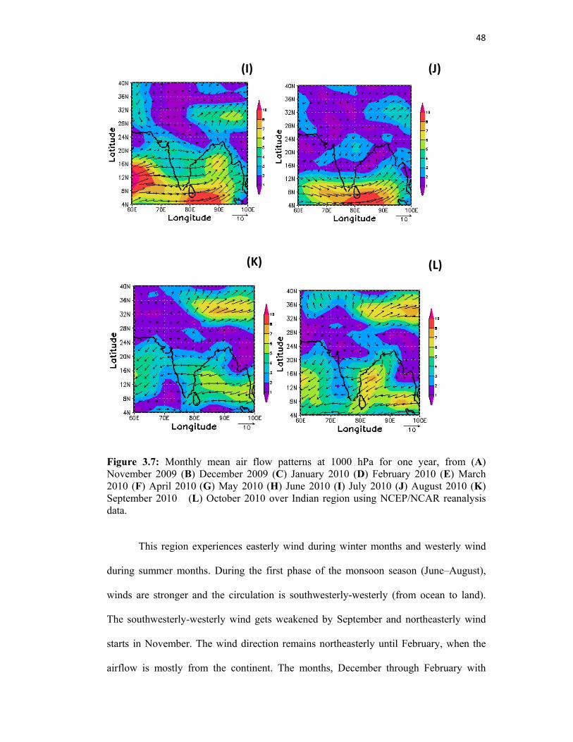
and lightning. Figure 3.7 shows the monthly mean air flow pattern at 1000 hPa in the
range 4°N-40°N latitude and 60°E to100°E longitude observed during the study period.
The wind pattern was obtained from the National Centers for Environmental Prediction/
National Center for Atmospheric Research (NCEP/NCAR) reanalysis data
(http://www.esrl.noaa.gov/psd/data/gridded/reanalysis/).
(B) (A)

47
(C) (D)
(F) (E)
(H) (G)
48
Figure 3.7: Monthly mean air flow patterns at 1000 hPa for one year, from (A) November 2009 (B) December 2009 (C) January 2010 (D) February 2010 (E) March 2010 (F) April 2010 (G) May 2010 (H) June 2010 (I) July 2010 (J) August 2010 (K) September 2010 (L) October 2010 over Indian region using NCEP/NCAR reanalysis data.
This region experiences easterly wind during winter months and westerly wind
during summer months. During the first phase of the monsoon season (June–August),
winds are stronger and the circulation is southwesterly-westerly (from ocean to land).
The southwesterly-westerly wind gets weakened by September and northeasterly wind
starts in November. The wind direction remains northeasterly until February, when the
airflow is mostly from the continent. The months, December through February with
(J) (I)
(L) (K)

49
meager rain and relatively low humidity constitute the winter season at this site, while
from March to May high convective movement persists and intense sun scorches the
surface. The period from December to March records the maximum sunshine hours of
more than 9.1 hours/day due to the clear sky and the minimum from June – August due
to cloudy sky conditions.
3.6 Results and discussion
About eighteen observations of AOD have been made on each clear sky day, in
between 09:00 hrs and 05:00 hrs. On most of the occasions, the measured AOD exhibit
diurnal variations, day to day variations and monthly variations.
3.6.1 Diurnal variations in AOD
The temporal variations in columnar AOD at different wavelengths observed on a
clear sky day (February 2010) are shown in figure 3.8 (a). It is found that the AOD at
lower wavelength is much higher than that obtained for higher wavelength. This
variation features can be attributed to the abundance of fine mode particles of continental
origin. It is also evident that the AOD shows a temporal variation with higher values in
the morning and late afternoon. It may be due to the high relative humidity as depicted in
figure 3.9. The peak observed in AOD during the mid-day hours could be attributed to
the local convective activity leading to change in aerosol particle number distributions.
Moreover, a sharp enhancement in AOD was found during 1530 hr (IST) at 340 nm,
which is due to the horizontal advection of pollution leading to higher aerosol column
content. On the other hand, a slight enhancement in AOD observed in other three
wavelengths (675, 870 and 1020 nm) found in the afternoon hours reveals the influence
of wind over this region. These results are in general agreement with those reported

50
earlier by different investigators at various coastal stations in India (Pinker et al., 1994;
Devara et al., 1996; Latha and Badarinath, 2005; Suresh and Elgar, 2005). In order to
validate our observation, the diurnal variation of direct solar flux at these wavelengths is
shown in figure 3.8(b).
Time (IST)
9 10 11 12 13 14 15 16 17
Aero
sol O
ptic
al D
epth
0.1
0.2
0.3
0.4
0.5
0.6
0.7(a)
(b)(b)
9 10 11 12 13 14 15 16 17
Sol
ar fl
ux (W
/m2 )
0
3
6
9
12
15
18340 nm 440 nm 675 nm870 nm 1020 nm
340 nm 440 nm 675 nm870 nm 1020 nm
Figure 3.8: Diurnal variation of (a) AOD (b) solar flux for different wavelengths
Since the observation site is away from National highway and industrial areas, the
aerosol variations are mainly influenced by the seasonal long range transport. This is

51
substantiated by air mass trajectory analysis which reveals that the observations were
influenced by both land and ocean in the month of February.
0
1
2
3
4
5
6
01234560
1
2
3
4
5
6
030
60
90
120
150180
210
240
270
300
330
(a)
2 4 6 8 10 12 14 16 18 20 22 24
Rel
ativ
e hu
mid
ity (%
)
40
45
50
55
60
(b)
Time (IST)2 4 6 8 10 12 14 16 18 20 22 24
Tem
pera
ture
(oC
)
21
24
27
30
33
36
(C)
Maximum RHMinimum RH
Maximum temperatureMinimum temperature
Figure 3.9: Diurnal variations of (a) maximum and minimum relative humidity (b) maximum and minimum temperature (c) wind speed and wind direction at Kannur in February 2010

52
The diurnal variation follows similar pattern in almost all the days. The variations for a
typical day on different months are depicted in figure 3.10.
January
9 10 11 12 13 14 15 16 170.0
0.1
0.2
0.3
0.4
0.5
0.6
0.7
February
9 10 11 12 13 14 15 16 170.0
0.1
0.2
0.3
0.4
0.5
0.6
0.7
March
9 10 11 12 13 14 15 16 170.0
0.1
0.2
0.3
0.4
0.5
0.6
0.7
April
9 10 11 12 13 14 15 16 17
Aero
sol O
ptic
al D
epth
0.0
0.1
0.2
0.3
0.4
0.5
0.6
0.7
May
9 10 11 12 13 14 15 16 170.0
0.1
0.2
0.3
0.4
0.5
0.6
0.7
September
9 10 11 12 13 14 15 16 17 180.0
0.1
0.2
0.3
0.4
0.5
0.6
0.7
October
9 10 11 12 13 14 15 16 170.0
0.1
0.2
0.3
0.4
0.5
0.6
0.7November
Time (IST)9 10 11 12 13 14 15 16 17
0.0
0.1
0.2
0.3
0.4
0.5
0.6
0.7
December
9 10 11 12 13 14 15 16 170.0
0.1
0.2
0.3
0.4
0.5
0.6
0.7
330 nm 440 nm675 nm 870 nm
1020 nm
340 nm 440 nm675 nm 870 nm
1020
340 nm 440 nm675 nm 870 nm
1020 nm
340 nm
440 nm
675 nm870 nm1020 nm
340 nm
440 nm
675 nm870 nm1020 nm
340 nm 440 nm
675 nm870 nm1020 nm
340 nm440 nm675 nm 870 nm
1020 nm
340 nm 440 nm675 nm 870 nm
1020 nm
340 nm
440 nm
675 nm
870 nm1020 nm
Figure 3.10: The diurnal variation in columnar AOD at different wavelengths observed on typical days in 2010
3.6.2. Monthly and seasonal variations in AOD
The monthly mean value and standard deviation of AOD at five wave lengths are
given in table 3.1. From the table, it is revealed that the mean values of AOD at all
wavelengths are high during April-May and low during November-December. It is
further observed that AODs were fairly high in summer (March-May), moderate in
monsoon (June-November) and low in post monsoon and winter seasons (December-
February).

53
Month & Year
AOD at different wavelengths (nm) Standard deviation of AOD at different wavelengths
340 440 675 870 1020 340 440 675 870 1020 Nov 09 0.337 0.208 0.131 0.098 0.09 0.022 0.021 0.021 0.021 0.020 Dec 09 0.365 0.205 0.132 0.09 0.081 0.027 0.027 0.050 0.025 0.026 Jan 10 0.420 0.293 0.196 0.159 0.146 0.032 0.025 0.020 0.019 0.018 Feb 10 0.428 0.260 0.195 0.122 0.108 0.038 0.026 0.022 0.018 0.012 Mar 10 0.466 0.274 0.221 0.133 0.120 0.040 0.030 0.025 0.021 0.020 Apr 10 0.512 0.401 0.308 0.162 0.129 0.080 0.055 0.043 0.041 0.032 May10 0.491 0.356 0.256 0.202 0.197 0.060 0.041 0.035 0.031 0.029 Jun 10 0.419 0.328 0.232 0.175 0.178 0.040 0.030 0.029 0.021 0.024 Aug 10 0.395 0.281 0.213 0.162 0.158 0.035 0.026 0.021 0.019 0.018 Sep 10 0.404 0.302 0.214 0.164 0.159 0.040 0.029 0.025 0.020 0.019 Oct 10 0.399 0.282 0.201 0.174 0.169 0.035 0.028 0.023 0.019 0.021 Nov 10 0.358 0.229 0.132 0.180 0.103 0.022 0.021 0.019 0.017 0.013 Dec 10 0.388 0.236 0.148 0.103 0.100 0.020 0.015 0.014 0.013 0.011 Jan 11 0.412 0.218 0.147 0.130 0.110 0.031 0.024 0.021 0.019 0.014 Feb 11 0.439 0.253 0.177 0.139 0.132 0.036 0.026 0.022 0.020 0.017 Mar 11 0.470 0.288 0.203 0.150 0.133 0.039 0.031 0.024 0.021 0.019 Apr 11 0.514 0.398 0.306 0.164 0.127 0.075 0.061 0.052 0.043 0.032 May 11 0.429 0.305 0.214 0.139 0.125 0.070 0.054 0.048 0.032 0.031 Jun 11 0.425 0.333 0.237 0.198 0.175 0.050 0.040 0.030 0.022 0.022 Aug 11 0.402 0.297 0.211 0.158 0.152 0.042 0.037 0.021 0.019 0.018 Sep 11 0.306 0.209 0.176 0.133 0.131 0.039 0.025 0.020 0.016 0.016 Oct 11 0.347 0.205 0.164 0.136 0.131 0.030 0.025 0.021 0.015 0.017 Nov 11 0.366 0.223 0.188 0.150 0.146 0.021 0.019 0.015 0.013 0.011 Dec 11 0.347 0.208 0.133 0.107 0.099 0.021 0.013 0.012 0.010 0.009 Jan 12 0.402 0.248 0.158 0.117 0.107 0.030 0.025 0.018 0.015 0.014 Feb 12 0.449 0.272 0.198 0.128 0.107 0.031 0.024 0.019 0.015 0.012 Mar 12 0.466 0.274 0.224 0.138 0.123 0.040 0.031 0.029 0.021 0.019 Apr 12 0.501 0.402 0.305 0.161 0.128 0.080 0.064 0.042 0.032 0.030 May 12 0.499 0.365 0.264 0.178 0.138 0.050 0.045 0.035 0.029 0.021
Table 3.1: Monthly mean aerosol optical depth with standard deviation
Monthly variations of AOD during the observation period and spectral average monthly
variation of AOD are depicted in figure 3.11 and 3.12 respectively. The vertical bars in
these figures represent one sigma standard deviation. Figure3.11 shows that the
minimum AOD is observed in December while the maximum is in April for all
wavelengths.

54
MonthN D J F M A M J J A S O N D J F M A M J J A S O N D J F M A M
Aer
osol
Opt
ical
Dep
th
0.0
0.2
0.4
0.6
0.8340nm440 nm
675 nm870 nm
1020 nm
2010 2011 20122009
Figure 3.11: Monthly variations in AOD with standard deviation
The average AOD at 340 nm is 0.38 ± 0.02 in winter, 0.48 ± 0.03 in summer, and 0.387
± 0.02 in monsoon. For 675 nm it is 0.148 ± 0.03 in winter, 0.244 ± 0.03 in summer,
0.206 ± 0.02 in monsoon whereas for 1020 nm it is 0.104 ± 0.02 in winter, 0.133 ± 0.04
in summer, 0.156 ± 0.05 in monsoon. Figure 3.13 shows the seasonal variation of aerosol
optical depth. The low value of AOD in post monsoon and winter seasons may be due to
the clear sky environment resulting in the settling of aerosols due to the rain washout
process. Moreover in winter months, the atmospheric boundary layer is shallow which
ensures a minimum mixing volume for the suspended particles. Since the humidity is
low, the marine aerosols cannot uptake water and grow in size. But in summer months,
the boundary layer height is higher and therefore pollutants have additional volume for
scattering and absorption of solar radiations passing through them. The influence of air
mass movement from the western side of this location indicates a strong marine
influence during pre-monsoon and monsoon seasons.

55
MonthN D J F M A M J J A S O N D J F M A M J J A S O N D J F M A M
Aer
osol
Opt
ical
Dep
th
0.0
0.1
0.2
0.3
0.4
Figure 3.12: Monthly spectral average variation of aerosol optical depth
The marine hygroscopic aerosols can uptake water and its subsequent growth in size
influences the intensity of solar and terrestrial radiations received on the surface
(Moorthy et al., 2005).
Wavelength300 400 500 600 700 800 900 1000 1100
Aer
osol
Opt
ical
Dep
th
0.0
0.1
0.2
0.3
0.4
0.5
0.6
0.7WinterSummer
MonsoonPost monsoon
Figure 3.13: Seasonal variations in aerosol optical depth

56
3.6.3 Monthly variations of Angstrom parameters α and β
Variations in the Angstrom parameters associated with light scattering by
aerosols are used to classify the abundance of fine and coarse mode particles. The
Ångström wavelength exponent α and turbidity coefficient β are derived from the ln τ –
ln λ plot, in which λ is expressed in µm. Monthly average values of α and β computed
from the linear fit and shown in table 3.2. The second order polynomial fit obtained
according to eqn (7) between ln τ and ln λ provides better agreement with measured
AODs rather than a linear fit. The norm of residuals for the polynomial fit is found to be
an order of magnitude less than that of the linear fit during the nine months from April to
January. Monthly average values of a2, a1 and α computed from the polynomial fit are
also shown in table 3.2. The ratios between AOD observed at 1020nm and at the other
four wavelengths (340nm, 440nm, 675 nm and 870nm) are shown in figure 3.14. Larger
ratios obtained for wavelengths 340, 440, 675 and 870nm during May-October indicate
the abundance of coarse mode particles.
MonthJan Feb Mar Apr May Jun Jul Aug Sep Oct Nov Dec
Rat
io o
f AO
D's
0.0
0.2
0.4
0.6
0.8
1.0
1.2
1.41020 nm/340 nm 1020 nm/440 nm1020 nm/675 nm 1020 nm/870 nm
Figure 3.14: Ratio of Aerosol optical depth

57
Month Linear fit Polynomial fit α β R2 (a1) (a2) α = (a2 –a1) β R2
Nov 09 1.11 0.08 0.96 -0.45 0.67 1.116 0.08 0.99 Dec 09 1.3 0.078 0.97 -0.83 0.45 1.276 0.082 0.98 Jan 10 1.26 0.09 0.96 -0.55 0.66 1.21 0.10 0.99 Feb 10 1.21 0.11 0.96 -1.15 0.05 1.20 0.11 0.94 Mar 10 1.18 0.12 0.94 -1.14 0.04 1.18 0.12 0.92 Apr 10 1.25 0.15 0.91 -2.23 -0.94 1.30 0.13 0.96 May 10 0.74 0.20 0.91 -0.29 0.5 0.78 0.20 0.98 Jun 10 0.72 0.18 0.91 -0.33 0.44 0.77 0.18 0.97 Aug10 0.67 0.16 0.93 -0.39 0.33 0.72 0.16 0.96 Sep 10 0.76 0.17 0.93 -0.38 0.43 0.80 0.17 0.98 Oct 10 0.68 0.17 0.87 -0.15 0.60 0.75 0.17 0.99 Nov 10 1.14 0.09 0.96 -0.34 0.76 1.09 0.10 0.99 Dec 10 1.23 0.09 0.96 -0.62 0.58 1.19 0.09 0.99 Jan 11 1.1 0.11 0.87 -0.09 0.96 1.04 0.11 0.95 Feb 11 1.05 0.12 0.93 -0.24 0.87 1.11 0.12 0.98 Mar 11 1.11 0.13 0.97 -0.74 0.34 1.08 0.13 0.98 Apr 11 1.24 0.15 0.91 -2.24 -0.95 1.29 0.13 0.96 May 11 1.11 0.13 0.09 -1.21 -0.10 1.106 0.12 0.98 Jun11 0.88 0.17 0.91 -0.89 0.001 0.885 0.16 0.86 Aug11 0.90 0.15 0.98 -0.65 0.23 0.883 0.15 0.99 Sep11 0.75 0.14 0.93 -0.39 0.33 0.72 0.13 0.92 Oct11 0.83 0.12 0.89 -0.01 0.77 0.78 0.13 0.94
Nov 11 0.78 0.14 0.88 -0.11 0.62 0.78 0.14 0.92 Dec 11 1.11 0.09 0.95 -0.35 0.73 1.07 0.11 0.91 Jan 12 1.18 0.13 0.98 -0.64 0.52 1.15 0.10 0.99 Feb 12 1.24 0.11 0.97 -1.2 0.06 1.24 0.11 0.96 Mar 12 1.19 0.13 0.94 -1.05 0.09 1.13 0.13 0.94 Apr 12 1.23 0.14 0.91 -2.27 -0.97 1.3 0.13 0.96 May12 1.12 0.14 0.98 -1.54 -0.36 1.144 0.14 0.99
Table 3.2: Monthly means value of wavelength exponent (α) and the turbidity coefficient (β) using linear fit and polynomial fit.
The (a2-a1) values can be approximated to alpha values as suggested by Eck et al.,
(1999) which is fruitfully validated by the correlation analysis (Praseed et al., 2012b). It
is found that there exists a strong correlation (R2 = 0.92) between (a2-a1) values and α
values retrieved from linear fit as shown in figure 3.15.

58
correlation coefficient (R2) =0.92
alpha0.6 0.8 1.0 1.2 1.4 1.6 1.8
(a2-
a 1)
0.6
0.8
1.0
1.2
1.4
1.6
Figure 3.15: Correlation between (a2-a1) and α
The monthly variations of α and β are shown in figure 3.16 and this reveals an inverse
relationship between α and β values.
MonthN D J F M A M J J A S O N D J F M A M J J A S O N D J F M A M
Ang
stro
m p
aram
eter
(α)
0.0
0.2
0.4
0.6
0.8
1.0
1.2
1.4
1.6
Turbidity factor ( β)
0.00
0.05
0.10
0.15
0.20
0.25Alpha Beta
Figure 3.16: Seasonal variations of α and β

59
Such a trend has been reported from many other observational sites in India and
elsewhere (Dani et al., 2003; Devara et al., 2005; Satheesh et al., 2006; Xin et al., 2007;
Madhanvan et al., 2008, Ganesh et al., 2008; Kumar et al., 2009; Sharma et al., 2011).
During the observation period, it was found that angstrom wavelength exponent α varies
in between 0.7 and 1.3.
The polynomial fit between lnτ and lnλ provides further microscopic insight into
aerosol size distribution. Significant variation was observed in a1 and a2 values (table
3.2); a1 varies from -0.15 to -2.23 and a2 values range from -0.94 to 0.76. In most of the
cases the coefficient a2 was positive, implying the dominance of coarse mode aerosols. A
negative value of a2 represents the domination of fine mode aerosols, and was observed
for the month of April-May. Similar negative curvatures were reported from the tropical
Indian coastal station Vishakhapatnam, during pre monsoon and summer monsoon
periods (Madhavan et al., 2008). The polynomial fit analysis indicates that the region is
influenced by both fine and coarse mode aerosols during February and March. But the
concentration of fine mode aerosol dominates during April and it continues till monsoon
activities are strengthened. Consequently during monsoon seasons this location is under
strong marine influence and the aerosols are mainly coarse in nature.
The air mass trajectory estimated using the HYSPLIT model during the period of
observation are shown figure 3.4 of section 3.4 From this, it is obvious that the air mass
movement during winter (December through February) and summer (March and April) is
from east of this site, and during monsoon (June to August) and post monsoon
(September to Early November) is from the western Arabian Sea. Further, during both
winter and summer seasons, long range transport of continental air mass contributes to
the observed AOD values, as the air masses appear to originate from the eastern part of

60
Kannur. Hence, it is presumed that this region is influenced by the transport of pollutants
from industrialised region during winter and summer. As the experimental site is far
from the industrial sources, the occurrence of fine-mode aerosol particles, on most of the
observation days, could be due to long-range transport of aerosols from distant source
regions. During the monsoon and post monsoon seasons, the movement of air mass
trajectories originated over the Arabian Sea. As the air mass passed over the Arabian
Sea, marine aerosols which are coarse in nature dominated at the lower level. Thus the
air trajectory analysis further validates our conclusion regarding the seasonal variation of
aerosols
3.6.4 Analysis of abrupt enhancement of AOD in festival occasions
During our three year long period of observations, it was found that the variations
in AODs were smooth, except during the months of April and May. Analysis of the
results further revealed a sudden change in AOD, alpha and beta values during the
burning of crackers associated with Vishu festival. Variations of AOD on pre and post
Vishu episode is shown in the figure 3.17. The increase was found to be more in the
lower wavelength region. The month April is earmarked with celebrations of festivals in
Kannur District. Moreover, Vishu a major festival in Kerala falls on 14th or 15th of April
every year. In north Kerala Vishu is celebrated with coordinated fireworks starting from
the eve of Vishu to 2-3 days after it. Such continuous fireworks from majority of houses,
public places and temples impair air quality (Attri et al., 2001) Nishanth et al., (2012a)
reported the enhancement of organic and inorganic particulate matter in the atmosphere
as a result of Vishu episode over Kannur. The variation of AOD and particle size
distribution before and after Vishu festival was precisely analyzed with the aid of second
order polynomial fit to ln λ versus ln τ graph.

61
Wavelength (nm)300 400 500 600 700 800 900 1000
Aer
osol
Opt
ical
Dep
th
0.1
0.2
0.3
0.4
0.5
0.6Pre-Vishu Post-Vishu
Figure 3.17: Variation of aerosol optical depth in the Vishu episode
Table 3.3 shows the mean AOD, alpha and beta values, coefficient of variation (C.V.)
(standard deviation/mean), calculated value of Students t test and one tailed p value
during the pre-Vishu and post Vishu days.
Event Wavelength (nm)
Alpha Beta 340 440 625 870 1020
Pre-Vishu 0.438 0.269 0.185 0.146 0.136 1.02 0.1305
Post-Vishu 0.523 0.387 0.296 0.158 0.14 1.28 0.143
C.V(pre-Vishu) 0.033 0.042 0.066 0.086 0.083 0.081 0.090
C.V(post-Vishu) 0.074 0.065 0.091 0.137 0.118 0.055 0.086
Value of ‘t’ -5.04 -10.5 -9.2 -1.1 -0.05 -6.04 -1.90
P value (one tailed) 0.00035 1.13E-06 2.91E-06 0.135 0.029 7.36E-05 0.041
Table 3.3: The mean AOD, alpha and beta values, coefficient of variation, calculated value of Students t test and one tailed p value in the pre-Vishu and post Vishu days

62
The positive curvature in the pre-phase (figure 3.18) and negative curvature in the post-
phase of Vishu (figure 3.19) indicates the domination of fine mode aerosols over coarse
mode during firework festivals.
Figure 3.18: ln λ vs ln τ (pre-Vishu) norm of residuals for linar fit is 0.18 and for polynomial fit=0.082
Figure 3.19: ln λ vs ln τ (post-Vishu) norm of residuals for linar fit is 0.28 and for polynomial fit is 0.18

63
This change in curvature may be due to the injection of fine mode particulate matter in to
the air. Nishanth et al., (2012a) has reported an increase of PM10 from 56 µg m-3 to 118
µg m-3 as a consequence of firework burning in April 2011. Student’s t-test value and
one tailed-p value reveals that, the enhancement of AOD in lower wavelength region is
statistically significant to 95% confidence level. The higher value of coefficient of
variation indicates that the aerosol variability is quite pronounced in the post Vishu
period. The smoke from fireworks comprising mainly of fine particles that can cause
respiratory problems and serious health issues (Uno et al., 1984).
3.7 AOD measurements in other geographical locations
Aerosol characteristics vary with geographical locations as well. The
concentration may vary over urban, rural, coastal and high altitude locations because of
the geography of the environment. In this section we present the results of the field
campaign measurements using MICROTOPS II over Ootty, a high altitude station in
south India; Trivandrum, a coastal site and Ahmadabad an urban site surrounded by
adjacent industrial areas.
Ootty, (11.3oN, 76.7oE) is a hill station at an altitude of 2240m above MSL,
generally lying in the boundary layer during day time and getting transformed into a
region of free troposphere during night time. The observation site Doddabetta peak, the
highest in the Nilagiri Mountains, is free from industrial and anthropogenic activities.
Hence a free troposphere exists here which is free from hectic convective activities. The
temperature is relatively low throughout the year, with average high temperature ranging
from 17-20oC and low temperature between 3-10oC. The average rain fall is about
1250mm with drizzling throughout the year and the weather is quite pleasant in March.

64
The AOD measurements were conducted during the second week of February 2011 since
the maximum number of clear sky days is available in February.
Ponmudi (8.72oN, 77.15oE) another pristine location, is a hill station lying 61 km
North East of Trivandrum city at an altitude of 1100 m. This hill region is a part of
Western Ghat Mountains and is now transformed into a tourist spot in the state. As a part
of exploring air quality over Trivandrum, AOD measurements were carried out at
Ponmudi, in the month of March 2011.
Trivandrum (8.54oN, 77oE) the capital city of Kerala State is located on South
West coast of India which is close to the extreme south of the Indian subcontinent. The
city has a tropical climate and therefore this location does not experience distinct
seasons. The maximum mean temperature is about 34oC and minimum 21oC. Being a
coastal site the humidity is high which rise to about 90% during monsoon seasons. The
city enjoys about 1700 mm of rain per year. North East monsoon is more active at
Trivandrum compared to other regions of Kerala. December-February is the winter
season with coldest months, while March-May is the hottest period. The observations
were carried out near Veli, 12 km away from Trivandrum city in the second week of
March 2011.
AOD measurements were carried out at Kannur town, the headquarters of Kannur
District. The observation site was on the top of Science Park which is 500m away from
the Arabian Sea shore, and close to the National highway (NH 17). The measurements
were carried out in the fourth week of March 2011.
Ahmadabad (23.2oN, 72.53oE) 55 m above MSL is located on the banks of
Sabarmathi river in Gujarat State and the AOD were measured at Physical Research
Laboratory Campus. The city is surrounded by sandy and dry area. The weather is hot
through the months of March-June. The average summer maximum temperature goes up
65
to 40oC and minimum 26oC, and during November - February the average maximum
temperature is about 30oC and minimum 14oC. The average rainfall over this location is
about 900 mm. It is polluted by adjacent industrial areas and textiles mills. The
measurements were carried out during the first week of April 2011.
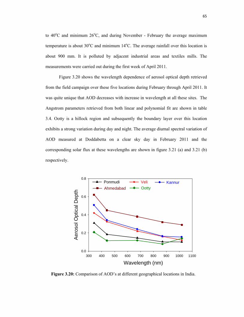
Figure 3.20 shows the wavelength dependence of aerosol optical depth retrieved
from the field campaign over these five locations during February through April 2011. It
was quite unique that AOD decreases with increase in wavelength at all these sites. The
Angstrom parameters retrieved from both linear and polynomial fit are shown in table
3.4. Ootty is a hillock region and subsequently the boundary layer over this location
exhibits a strong variation during day and night. The average diurnal spectral variation of
AOD measured at Doddabetta on a clear sky day in February 2011 and the
corresponding solar flux at these wavelengths are shown in figure 3.21 (a) and 3.21 (b)
respectively.
Wavelength (nm)300 400 500 600 700 800 900 1000 1100
Aer
osol
Opt
ical
Dep
th
0.0
0.2
0.4
0.6
0.8Ponmudi Veli KannurAhmedabad Ootty
Figure 3.20: Comparison of AOD’s at different geographical locations in India.

66
The AODs’ are quite low compared to that measured at KUC. It is further noticed that
the AOD at 340 nm shows a dramatic increase in the afternoon due to the intense
convective actives on the valley which induces a vertical air mass movement. Hence the
asymmetry between the FN and AN AOD’s is the highest in Ootty. Likewise, the
enhancement of AOD in higher wavelengths is quite pronounced at this site due to the
presence of fog in the atmosphere. The higher value of AOD at 1020 nm indicates the
abundance of coarse aerosols over this region. One of the special observations found is
the enhancement of AOD at 1020 nm over the AODs at 440, 675 and 870 nm. This is an
indication of low level clouds and haze over this hill station throughout the day. The
reason for higher magnitudes of AODs observed in the afternoon may be attributed to the
long range transport of aerosols from surrounding valley.
Backward air trajectory at Ooty (February 2011) during forenoon and after noon are
shown in the figure 3.22 (a) and 3.22 (b) respectively.
Date Place Linear fit Polynomial fit
α β R2 (a1) (a2) α =
(a2–a1) β R2
14th Feb Ootty 0.49 0.09 0.55 14th Mar Ponmudi 0.97 0.11 0.96 -0.55 0.43 0.98 0.10 0.96 16th Mar Veli (Tvm.) 1.09 0.13 0.98 -1.52 -0.39 1.13 0.13 0.99 28th Mar Kannur 1.27 0.15 0.97 -0.86 0.39 1.25 0.15 0.97 5th April Ahmedabad 0.64 0.29 0.96 -0.45 0.17 0.62 0.31 0.96
Table 3.4: Angstrom parameters (α and β at different locations in India)
At Veli (Trivandrum), the coastal site which is free from hectic anthropogenic activities,
the aerosol loading is higher (β=0.13) than that at Ponmudi, the hill station 61 km east of
Trivandrum city. The low negative value of a2 (-0.39) is an indication of equal
contribution of both fine and accumulation mode. Being the air mass flow is from the

67
eastern side, (figure 2.23.a) it has to travel a long distance over the land before reaching
the observation site. Thus this air flow through the thickly populated regions can
contribute to fine and accumulation mode aerosol through secondary production
mechanism in the warm and humid tropical environment. Ponmudi a high altitude site
has a clean atmosphere. But the recent tourist activities and rapid urbanization induce
possible threats to the air quality.
(a)
9 10 11 12 13 14 15 16 17
Aer
osol
Opt
ical
Dep
th (A
OD
)
0.00
0.05
0.10
0.15
0.20
0.25
0.30
0.35
(b)
Time (IST)9 10 11 12 13 14 15 16 17
Sol
ar fl
ux (W
/m2 )
0
3
6
9
12
15
18
21
340 nm 440 nm 675 nm 870 nm 1020 nm
340 nm 440 nm 675 nm 870 nm 1020 nm
Figure 3.21: Diurnal variation of (a) AOD and (b) solar flux for different wavelengths at Ooty

68
Figure 3.22: Air mass trajectory analysis at Ootty (a) Forenoon (b) Afternoon
Figure 3.23: Air mass trajectory analysis (a) at Veli (b) at Ponmudi
The aerosol loading at Ponmudi is low (β = 0.11) as compared to Trivandrum. The air
trajectory analysis (figure 3.23.b) further shows that the long range transport is from the
eastern side and air mass travels comparatively short distance over land mass before
reaching the observation site. The relatively high values of α (1.27) and a2 value of 0.39,
observed over Kannur town indicate a slight abundance of fine mode aerosols of
anthropogenic origin over coarse mode. This may be due to vehicular emission and fine
dust particles produced due to the deteriorated road conditions. The air trajectory
analysis (figure 3.24a) indicates that the region has a mixed influence of land and ocean.

69
At low level, near the surface, the air mass flow is from the Arabian Sea, which brings
marine aerosols over this region, whereas at 1500m altitude, the effluents is mainly from
the land, which brings industrial pollutants to this region. The low positive a2 value
clearly validates the presence of bimodal aerosol. As we presumed, Ahmadabad shows
high aerosol concentration owing to its industrial developments. The high β value (0.31)
is an indication of dense aerosol loading whereas the low α value (0.64) designate coarse
mode particles.
Figure 3.24: Air mass trajectory analysis (a) at Kannur town (b) Ahmadabad
The dust particles and pollution transported (figure 3.24b) from nearby industrial areas
may further deteriorate the air quality of this region. The conversion of fine to
accumulation mode dust particles, due to secondary production mechanisms can be the
main contributors of coarse aerosols. Thus the results of the field campaign indicate, low
values of AOD over Ootty, and very high value over Ahmadabad, and moderate value
over Trivandrum as expected. The high value of AOD found over Kannur town than at
KUC is really disturbing; and shows the influence of vehicular emission and local
industries on aerosol concentration.