chapter 32 - home | w. w. norton & company chapter 32 trade unions ii: collective bargaining and...
TRANSCRIPT

1
chapter 32Trade Unions II: Collective
Bargaining and Strikes
In Chapter 18, we provided a largely informal account of trade union behavior. There, the focus was on understanding the determinants of union density and the impact of unions on labor-market outcomes
(in particular, their effect on earnings, employment, worker productiv-ity, and profitability). In this one, we shift gears by presenting a more comprehensive microeconomic analysis of their behavior.1 As we shall see, this approach provides penetrating insights into both the nature of collective bargaining agreements and the reasons that the bargain-ing process occasionally breaks down, resulting in a strike, lockout, or some other form of industrial action.
In 2007, there were only 20 work stoppages in the United States, that involved more than 1,000 workers. In fact, the vast majority of negotia-tions between unions and employers are peaceable enough, leading to the successful hammering out of a contractual agreement between the two parties. This observation sets the stage for the material presented in Sections 32.1 and 32.2, in which we discuss the forces that shape the form of these agreements.
In Section 32.3, we then discuss strikes and lockouts. Despite their rarity, industrial disputes are often extremely disruptive for all parties involved: employers, workers, and customers. For instance the 2004–2005 lockout led to the cancellation of the entire ice hockey season and left countless numbers of despondent fans in its wake. Likewise, mem-bers of the traveling public were no doubt miffed to learn that, while they were stuck at home, their luggage was enjoying an extended vaca-tion in Hawaii—as a result of the Christmas 2004 industrial dispute by US Airway’s baggage handlers.
In the United States, many disputes legally must be resolved via a process of arbitration, which is the subject matter of Section 32.4. Arbi-tration is an especially common practice among public-sector unions,
L e a r n i n g O b j e c t i v e s
By reading this chapter, you should be able to:
• Understand the concept of a union contract and the nature of a union’s objectives.
• Recognize the basic tenets of the monopoly union model, and both the efficient contracting and strongly efficient contract-ing hypotheses.
• Understand the stylized facts concerning changes in the incidence of industrial disputes in the United States.
• Understand the Hicks paradox and be able to explain why strikes (and other forms of industrial action) may represent individually rational investments in information.
• Recognize why the inherent nature of the professional sports industry provides such fertile grounds for industrial disputes of one sort or another.
88147_WEB_ONLY_32_001-040_r2_ra.indd 1 5/17/11 12:00:01 PM

2 Chapter 32: Trade Unions II: Collective Bargaining and Strikes
since the law often prohibits strikes and lockouts. Section 32.5 closes by applying the material to help explain the rocky industrial-relations landscape of the profes-sional sports industry in the United States.
32.1 The Collective Bargaining EnvironmentUnions and firms engage in collective bargaining in order to hammer out an agreement on the terms of the contract that will govern their relationship over a prescribed interval of time (usually between 1 and 3 years). The principal goal of this and the next section is to identify the factors that determine the form of these agreements.2
Union ContractsUnion contracts vary in their complexity. At one extreme, some contracts are only 1 page long, and at the other some are over 800 pages long!3 Contracts can deal with almost any aspect of the employment relationship that firms or work-ers deem to be significant.4 Some deal with obvious concerns (such as wages and working conditions), while other provisions deal with less obvious ones such as the number of towels the firm is obliged to provide in the restrooms.
Be this as it may, we shall focus on the case in which the generic contract, v, includes only two items and takes the following simple form: v = (w, L), where w is the wage, and L is the level of union employment. (We refer to particular contracts by the uppercase letters A, B, C, and so on.) The focus on these two items reflects their first-order importance: put simply, workers care mostly about what they earn and whether they are employed! Of course, as just noted, unions and firms negotiate over many different items: the length of the shift, job secu-rity, health benefits, working conditions, and, of course, the number of towels in the restrooms. Nevertheless, equipped with a solid understanding of the choices of w and L, it is a relatively simple matter to extend the analysis to include these additional elements.
Union ObjectivesWhat does labor want? Samuel Gompers replied as follows:5
Labor wants more schoolhouses and less jails; more books and less arsenals; more learning and less vice; more constant work and less crime; more leisure and less greed; more justice and less revenge; in fact, more of the opportunities to cultivate our better natures.
As is apparent from this quotation (which is as relevant today as it was over 100 years ago), unions pursue a variety of goals: economic, social, and political.
88147_WEB_ONLY_32_001-040_r2_ra.indd 2 5/17/11 12:00:01 PM

32.1: The Collective Bargaining Environment 3
In the interests of simplicity, however, in this chapter we focus exclusively on their economic objectives.
Let’s consider a union that bargains on behalf of L work-ers and assume that union leaders are benevolent: they act in the interests of the union membership rather than pur-suing their own goals.6 Each member of the union derives utility, u, from consumption, c, according to u = u(c).
The relationship u(c) is assumed to be both increas-ing and concave in c (indicative of the diminishing marginal utility of consumption). Let’s assume that the union values each worker’s utility, u(c), and the level of union employment, L (which determines the union’s strength). We consider the simplest formulation in which the union’s utility, denoted U, equals the total util-ity of all L of its members:7
U = U(c, L) = L · u(c) (32.1)
In the interests of simplicity let’s assume that $w = $c, which implies each worker’s income, $w, equals his expenditures on consumption, $c. This is a reasonable enough approximation for most union workers since their earnings are their only source of income and hence consumption. In turn, this implies that the union’s utility can be written U = L · u(w). Figure 32.1 depicts the union’s preferences. The level of union employment, L, is depicted along the horizontal axis and the wage, $w (which equals each worker’s consumption level, $c) along the vertical one. Notice that each point in the figure corresponds to a particular contract v, so point A corresponds to the contract A = (w0 , L0).
Each of the indifference curves represents the locus of contracts that provides the union with the same level of utility. The negative slope of each curve is stan-dard and indicates the fact that the unions regards both L and w as goods. As shown, the union’s utility increases in the direction indicated by the arrow: it prefers both a greater level of employment and a greater wage for each of its members.8
The union and the firm negotiate over the terms of the contract, v = (w, L). The union’s objective is to select a contract, v, that maximizes its utility, U. Neverthe-less, a variety of constraints impede its choices. They arise from the party facing it on the other side of the bargaining table: the employer. It seeks to pursue its own profit-maximizing goals and operates within an environment that punishes failure with bankruptcy.
The Constraints: The EmployerFor simplicity, let’s consider a profit-maximizing firm that is a perfect competitor in the product market. Let p denote the product price and y = f (L) the production function. The firm’s profits are then π(w, L) ≡ p · f (L) − w · L.
U1
U2
U0
LL0
Greater utility
A w0
A = (w0, L0)
$w
FigUrE 32.1 Union Preferences
88147_WEB_ONLY_32_001-040_r2_ra.indd 3 5/17/11 12:00:02 PM

4 Chapter 32: Trade Unions II: Collective Bargaining and Strikes
In what follows, let MRPL denote the mar-ginal revenue product of labor. From now- familiar arguments, we know that the MRPL decreases with the level of employment, L, and that, under perfectly competitive condi-tions, the MRPL schedule is the firm’s labor-demand schedule.9
In Figure 32.2, we depict the firm’s MRPL schedule, together with an assortment of isoprofit curves. As the name perhaps sug-gests, each isoprofit curve represents a locus of contracts, v = (w, L), that generate an iden-tical level of profits $π.
The shape of each isoprofit schedule fol-lows from the fact that, for each given wage, the MRPL schedule governs the firm’s profit- maximizing employment level. To see why this is so, suppose that the wage is w0. As shown, the firm’s profits are maximized
at point A, where its optimal employment level is L0 and its maximized profits are π2. Because L0 maximizes the firm’s profits, given the wage w0 , it follows that any other employment level must lower them.
Accordingly, let π1 < π2 denote the profits that accrue to the firm if it chooses the employment level L′ (any value will do). This leads to point B, which lies on the isoprofit curve π1. Again starting at L0 (and holding the wage con-stant at w0), now suppose that we progressively increase the level of employment. For a suitable increase (as shown at L″) we can drive down the firm’s profits to exactly π1, which leads to point C on the isoprofit schedule π1. Finally, again starting from point A, now suppose that we gradually increase the wage and allow the firm to adjust its optimal level of employment (this exercise results in a movement along the MRPL schedule). As the wage increases, the firm’s maxi-mized profits gradually decline. As shown, its profits are driven down to exactly π1 at the wage w1. This exercise leads to point D on the isoprofit schedule π1. By connecting points B, D, and C we then arrive at the isoprofit schedule π1. Exactly the same principles that underlie the derivation of this isoprofit schedule apply to them all.
As indicated, the firm’s profits increase in the direction of the arrow; ceteris pari-bus, the lower the wage the greater the firm’s profits. The isoprofit locus π0 = 0 is particularly noteworthy since the firm’s profits are precisely zero. It represents the upper limit of what is achievable by the union. Pushing the firm any further kills the golden goose because the firm becomes insolvent.
Figure 32.2 also depicts the competitive wage, wc , which is the wage available to union workers elsewhere in the economy. Notice that at this wage the firm would,
LL0 Lc
w0
w1
wc
$w
MRPL
D
E
F
CB A
Greater
profi
ts
Union Employment
L′ L″
π0 = 0
π2
π2
π1
FigUrE 32.2 The Firm’s Isoprofit Curves
88147_WEB_ONLY_32_001-040_r2_ra.indd 4 5/17/11 12:00:03 PM
32.1: The Collective Bargaining Environment 5
in the absence of the union, maximize its profits by choosing the level of employ-ment Lc—as shown at point F, which lies on the labor-demand schedule.
More will be said about the competitive wage, wc , later. Suffice it to say, wc rep-resents the lower limit on the union’s contractual agreement. If the firm tries to force the union to agree to a wage that is less than this value, then individual union members can do better by seeking employment elsewhere—thus quitting both the union and the firm.
A comparison of Figures 32.1 and 32.2 immediately reveals the conflict of in-terest that arises between the union and the firm. Loosely speaking, the union seeks a contractual agreement that lies as far as possible in the northeast direction (to maximize its utility) and the firm, for its part, seeks one that lies in the oppo-site southeast direction (to maximize its profits). Yet, the two parties must reach a compromise, lest a strike or lockout ensue.
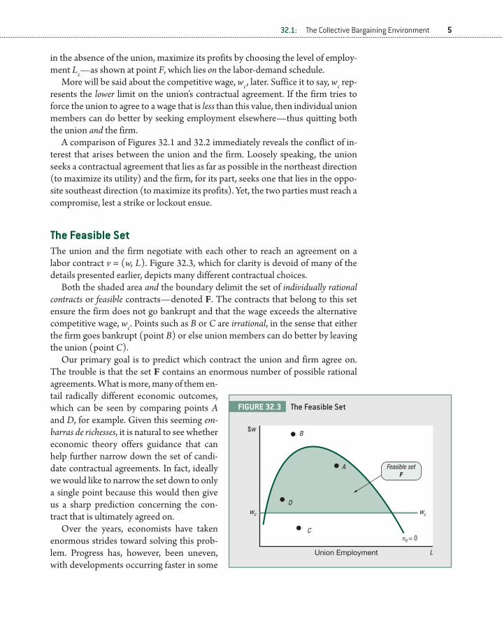
The Feasible SetThe union and the firm negotiate with each other to reach an agreement on a labor contract v = (w, L). Figure 32.3, which for clarity is devoid of many of the details presented earlier, depicts many different contractual choices.
Both the shaded area and the boundary delimit the set of individually rational contracts or feasible contracts—denoted F. The contracts that belong to this set ensure the firm does not go bankrupt and that the wage exceeds the alternative competitive wage, wc. Points such as B or C are irrational, in the sense that either the firm goes bankrupt (point B) or else union members can do better by leaving the union (point C).
Our primary goal is to predict which contract the union and firm agree on. The trouble is that the set F contains an enormous number of possible rational agreements. What is more, many of them en-tail radically different economic outcomes, which can be seen by comparing points A and D, for example. Given this seeming em-barras de richesses, it is natural to see whether economic theory offers guidance that can help further narrow down the set of candi-date contractual agreements. In fact, ideally we would like to narrow the set down to only a single point because this would then give us a sharp prediction concerning the con-tract that is ultimately agreed on.
Over the years, economists have taken enormous strides toward solving this prob-lem. Progress has, however, been uneven, with developments occurring faster in some
L
wc
$w
D
C
B
A
Union Employment
π0 = 0
wc
Feasible setF
FigUrE 32.3 The Feasible Set
88147_WEB_ONLY_32_001-040_r2_ra.indd 5 5/17/11 12:00:03 PM

6 Chapter 32: Trade Unions II: Collective Bargaining and Strikes
areas than in others. In fact, with the benefit of hindsight, it is evident that much of the terminology that remains in common use today is less than ideal. In what follows, we will try and alert the reader to potential difficulties.
32.2 The Contractual AgreementLet’s begin by considering the case of the so-called monopoly union model, since this was the one first studied by economists.
Monopoly Unions. In the case of a monopoly union, the negotiation process over the contract v = (w, L) is as described in Assumption 32.1.
A S S U M p T i O n 32 .1
Monopoly Unions(a) The union sets the wage, $w.(b) The firm responds to the union wage by choosing the level of employment, L.(c) After each party has made its decision, no further negotiations take place,
and the agreed contract v = (w, L) is implemented.
The union is a monopolist: it picks the wage, and the firm responds by choosing the number of union members to hire.
The union’s monopoly power stems from its control of the labor that is sup-plied by its members in general and its ability to withhold this supply from the
firm in particular.10 The union is assumed to be aware of the fact that the higher it sets the wage the lower is the firm’s demand for its labor. The trouble is that the union cares about both the wage and the level of employment.
Figure 32.4 depicts the monopoly union model’s solution. To understand the message it conveys, suppose that the union sets the wage w0 and that the firm responds by pick-ing the profit-maximizing level of employ-ment L0. As shown, this leads to the contract A = (w0 , L0), which provides the union with utility U0. Can the union do better than this outcome?
It can indeed! To see how, suppose that instead it sets the wage equal to wm and that the firm responds by picking the level of
LL0 LcLm
w0
wc
wm
$w
MRPL
M
C
B
A
UmU0
Union Employment
π0 = 0
πm
πm
D
FigUrE 32.4 The Monopoly Union
88147_WEB_ONLY_32_001-040_r2_ra.indd 6 5/17/11 12:00:04 PM

32.2: The Contractual Agreement 7
employment Lm. As shown, this leads to the contract M = (wm , Lm), which pro-vides the union an even greater level of utility: Um > U0.
Hence selecting w0 cannot be optimal from the union’s perspective because it is dominated by wm. Moreover, it is easy to see from the figure that, starting from wm , if the union either raises or lowers the wage, then its utility declines. This fact establishes that wm maximizes the union’s utility. Notice the solution is character-ized by a tangency condition: the union’s highest attainable indifference curve, Um , is tangent to the firm’s labor-demand schedule MRPL.
It follows that, according to the monopoly union model, the union and firm are predicted to agree to the contract M = (wm , Lm). As shown, the wage exceeds the competitive wage wm > wc , and the level of union employment is lower than that which would prevail in a competitive market, Lm < Lc.
Despite the simplicity, the monopoly union model suffers from certain fundamental—some would argue fatal—problems. The basic concern is rooted in Assumption 32.1c, which ruled out further negotiations after the firm picks its level of employment. Suppose, instead, that the firm can propose an alter-native contract to the union—and that no further negotiations take place after that. Can the firm make an offer that the union will find acceptable? The answer is that it can!
To see how, notice that all of the points in the interior of the green shaded lens MB are feasible contractual agreements that increase the well-being of both the firm and the union—when compared to point M. Consequently, the ability of the firm to make a counteroffer is sufficient to dislodge M as the solution to the union–firm bargaining problem. The basic concern for the monopoly union model is that it is entirely plausible to believe that unions and firms can and do make these kinds of offers and counteroffers as they bargain with each other.
If the monopoly model is implausible, are there other criteria that can be used to narrow down the set of possible bargaining agreements? Fortunately there are, and they form the subject matter of the rest of this section.
Efficient Contracts. A contract, v = (w, L), is simply a wage-employment com-bination. The precise characterization of an efficient contract is given in Defini-tion 32.1.11
DEFiniTiOn 32.1: Efficient ContractsAn efficient contract v = (w, L) is a contract that possesses the following two properties:(a) w ≥ wc and π(w, L) ≥ 0.(b) Every other feasible contract, v′ = (w′, L′), strictly lowers the utility of the union, the
profits of the firm, or both.
Condition 32.1a ensures the contract is potentially acceptable to both parties. For example, if π(w, L) < 0, then it is better for the firm to shut down rather than to accept the terms of the deal. Part (b) precludes the existence of some other
88147_WEB_ONLY_32_001-040_r2_ra.indd 7 5/17/11 12:00:04 PM

8 Chapter 32: Trade Unions II: Collective Bargaining and Strikes
contract that benefits one party without hurting the other. This latter point is the essence of the efficient-contracting approach. It ensures that if the firm and the union agree to some contract P, then there is no further scope for them to negoti-ate an even better deal that increases both their welfare levels.
The nature of the problem that is inherent in the monopoly union model fol-lows immediately from these remarks and from Definition 32.1. As shown in Figure 32.1, the agreed contract, M, is not efficient. Although it satisfies condi-tion (a) of Definition 32.1, it fails condition (b) because the contract represented by point D, for example, makes both the firm and the union better off.
Figure 32.5 depicts the feasible bargaining set, F, the union’s indifference curves, and the firm’s isoprofit curves. The contract curve, depicted by the line XY, plays an important role in the economic analysis of bargaining. As shown, it consists of the locus of tangency points between the firm’s isoprofit curves and the union’s indifference curves that lie either within the feasible bargaining set F or lie on its boundary (such as X and Y).
The importance of the contract curve XY stems from the remarkable facts that (i) every efficient contract lies along the contract curve and (ii) every con-tract that lies on the contract curve is efficient. In other words, the contract curve XY and the set of efficient contracts are essentially one and the same!12 Verifying part (i) of the claim is simple enough. Points that lie off the contract curve cannot be efficient. To see why, consider the generic contract represented by point D in the figure: it is feasible but lies off of the contract curve. It is easy enough to see, however, that this contract is not efficient for all of the contracts that lie within the
lens DBEA are also feasible and they increase both the firm’s profits and the union’s utility.
To see why claim (ii) is correct (every point on the contract curve is an efficient contract), consider, for example, the speci-men contract A depicted in the figure. There are potentially two ways of moving away from this point: movements along or off the contract curve. Evidently, movements along the contract curve strictly lower either the utility of the union or reduce the firm’s prof-its. Yet, it is readily seen that movements off the contract curve—such as to point D—do precisely the same thing. Thus, relative to point A, every other point in F makes either the firm or the union worse off, implying that point A is an efficient contract. Yet, what ap-plies to the specimen contract A applies with equal force to any other contract that lies on the contract curve XY.
L
wc
$w
DY
E
F
X
B
A
Union Employment
π0 = 0The contract curve
Isoprofit curves
Indifference curves
MRPL
FigUrE 32.5 The Contract Curve
88147_WEB_ONLY_32_001-040_r2_ra.indd 8 5/17/11 12:00:05 PM

32.2: The Contractual Agreement 9
The contract curve may be positively sloped, negatively sloped, and may even possess both positively sloped and negatively sloped segments (as in the case illustrated). Notice, however, the union’s indifference curves are negatively sloped and that the firm’s isoprofit curves are negatively sloped only to the right of the labor-demand curve. Consequently, the points of tangency between these sets of curves—and hence the contract curve itself—must lie to the right of the labor-demand curve MRPL.
This latter observation leads to one of the central predictions of the theory of efficient union contracts—namely, given any wage w, the profit-maximizing level of employment (which is governed by the MRPL schedule) is lower than that agreed under an efficient contract (which is governed by the contract curve XY). This excess employment prediction of the model is often invoked to explain union practices that fall under the general rubric of featherbedding.13 A short list of such practices includes the following:
Manning levels Manning levels are the requirement that a certain number of union members must be employed to perform a prescribed task.
Inflexible work practices There are many different instances of inflexible work practices. One of the most notorious of them is in which a union member is assigned to perform a narrow set of duties. For example, a mechanic might be assigned to the task of maintaining and repairing a particular piece of equip-ment in a steel plant. Consequently, if some other machine breaks down, the mechanic might be barred from repairing it—even if he or she is currently idle and is perfectly capable of doing so.
Unnecessary work In the early 1960s, over 30,000 firemen (the ones with the shovels not the yellow hats) were employed in America’s diesel powered railways—a remnant from the days of the coal-powered steam engine.
Taking stock, by focusing on efficient contracts the set of possible bargain-ing agreements collapses to the contract curve XY. Still, there are many—an infinity—of different contracts that lie along this curve. In Appendix 32.A we show how economic theory can help us predict which one will be chosen. For the moment, let’s turn our attention to the concept of strongly efficient contracts.
Strongly Efficient Contracts. Given that every efficient contract lies on the con-tract curve XY, the reader (understandably) may be quite flabbergasted to learn of the existence of strongly efficient contracts—which do not. In essence, the notion of strongly efficient contracts arises from two considerations: (i) a reevalu-ation of whether the union’s objective, U(c, L) = u(c) · L, is a reasonable one and (ii) the admission of a richer set of contracts.
As for point (i), recall that L is the level of union employment. An alternative viewpoint is that the union does not care about the level of employment per se; instead, it cares about the consumption of each of its members and its total
88147_WEB_ONLY_32_001-040_r2_ra.indd 9 5/17/11 12:00:05 PM

10 Chapter 32: Trade Unions II: Collective Bargaining and Strikes
membership (as distinct from their employ-ment). Put another way, if each of its 10,000 members has an income of $50,000, then the union may be indifferent concerning the details of how many of them are actually em-ployed.14 Figure 32.6 is used to explain the basic principles.
Once again, let’s consider a situation in which the firm and the union must negotiate a con tract. Likewise, there is an alternative competitive sector that offers the constant wage wc. In the figure, let’s strip away many details and simply depict the contract curve, XY, together with the monopoly union con tract, M, and the competitive—supply equals demand—outcome C.
To begin with, assume that the union and the firm agree to the efficient contract at point A in the figure (any point on XY will do). The contract lies on the contract curve and is characterized by the agreement (w0 , L0). Given this contract, the firm’s wage
bill—that is, the total amount paid by the firm to all of the members of the union—is given by $B0 = w0 · L0 , which equals the size of the rectangle formed by the areas I + II + III.
The basic idea behind a strongly efficient contract hinges on point 2 men-tioned earlier, which concerns the richness of the contract that is offered. In particular, we are now going to suppose that the firm (or the union) proposes a richer contract that includes more terms and takes advantage of employment op-portunities available in the competitive labor market.15 Moreover, the new offer is going to strictly increase the firm’s profits and not reduce the utility of any union member.
With this in mind, suppose that the firm first proposes reducing the level of employment from L0 to the competitive level Lc , and that it also proposes that those who are displaced work in the competitive industry at the wage of wc. As things stand, this would, of course, certainly attract the ire of the union because those union members who lose their jobs suffer an evident reduction in their incomes.
Pressing on, suppose, however, that the firm also proposes that (1) it will main-tain the wage at w0 for all employees, and (2) it will provide displaced workers with a top-up severance package of s0 = w0 − wc (see point E in the figure). In other words, the firm is proposing the new richer contract v = (w0 , L0 , s0), which now includes a provision for the severance payment, s0. Under the new contract, the
LLc L0
wc
w0
$w
Union Employment
MRPL
M
Y
C
S
II
III
X
Contract curve
Strongly efficient contracts
AE
I
π0 = 0
FigUrE 32.6 Strongly Efficient Contracts
88147_WEB_ONLY_32_001-040_r2_ra.indd 10 5/17/11 12:00:06 PM

32.2: The Contractual Agreement 11
utility of every union member remains unchanged.16 The firm’s new wage bill, B1 equals:
B1 = w0 · Lc + s0 · (L0 − Lc ) = w0 · Lc + (w0 − wc ) · (L0 − Lc ) (32.2)
Upon simple rearrangement Equation 32.2 gives:
B1 = B0 − wc · (L0 − Lc ) < B0 (32.3)
Hence the firm’s new proposed contract offer reduces its labor costs: B1 < B0. In fact, its costs decline by an amount equal to the area I + II depicted in the figure (the area III equals the value of severance payments made to those workers who are laid off).
Nevertheless, the proposed reduction in employment also lowers the firm’s revenues. They decline by an amount that equals the area I in the figure, which corresponds to the area under the MRPL schedule (i.e., the area under the firm’s labor-demand curve). But it is easy to see that the firm’s costs (areas I + II) decline by more than its revenues (area I). It follows that the proposed richer contract increases the firm’s profits by an amount that is equal in size to the area II.17
In short, the new contract strictly increases the firm’s profits and leaves the util-ity of every union member unchanged. Granted, the union may then propose a counteroffer to raise the utility of all of its members but, regardless of the details, we are clearly onto something! Specifically, starting at any point on the contract curve XY both the firm and every union member can be made strictly better off by moving to an appropriate point on the line CS, which is vertical, and, on exten-sion, runs through the competitive employment level Lc. The line CS is called the locus of strongly efficient contracts.
Some interesting predictions emerge from the strongly efficient contracting model. First, suppose the union’s bargaining power increases (following, for ex-ample, a favorable change in the legal environment), which allows it to negoti-ate a higher wage for its members. According to the strongly efficient contracting model, this change has no effect whatsoever on the level of employment, which remains fixed at the competitive level Lc. Second, with the level of employment pinned down at Lc , the firm’s revenues are also pinned down at R = p · f (Lc ). It follows that every additional $1 the firm pays to the union leads to an equal and opposite $1 decrease in its profits.
Each of the three union models presented in this section has quite distinct implications that can be used as a basis for empirically distinguishing them. Let MH, EH, SH stand for, respectively, the monopoly union hypothesis, efficient contracting hypothesis, and strongly efficient contracting hypothesis. Trammel-ing together the consequences of the discussion up to this point leads to the fol-lowing testable hypotheses: Bargaining power An increase in union bargaining power has no effect on wages
or employment under MH, raises the wage and affects employment under EH, and raises the wage but does not change employment under SH.18
88147_WEB_ONLY_32_001-040_r2_ra.indd 11 5/17/11 12:00:06 PM

12 Chapter 32: Trade Unions II: Collective Bargaining and Strikes
Stock-market value Following a ceteris paribus increase in the wage, the stock value of the firm declines under all three of the hypotheses. Nevertheless, only in the case of SH does each $1 increase in the earnings of union members re-duce the stock market value of the firm by precisely $1.19
The alternative wage A small exogenous increase in the competitive wage wc has no effect on the firm’s employment level under MH or EH, but reduces it under SH.Many studies have sought to empirically distinguish among the alternative hy-
potheses just described.20 A preponderance of the evidence indicates that union contracts tend to lie off the labor-demand curve—a finding that is potentially consistent with some form of efficient contracting (whether of the strong or weak varieties). As for distinguishing between EH and SH, here the evidence is rather mixed. However, some tests that are based on changes in the stock market value of unionized firms do point to the existence of strongly efficient contractual agreements.21
In this section, we have circumscribed the set of individually rational contrac-tual agreements. Nevertheless, despite the progress, a glaring problem remains to be solved. Only the monopoly union model predicts which contract the union and the firm will actually agree on. The efficient and strongly efficient contracting models only delimit a range of possible agreements that, respectively, lie along the XY and CS loci. The trouble is that no criteria have yet been advanced to isolate which one of these many possible contracts the union and the firm will ultimately choose. (This important topic is discussed in Appendix 32.A.)
32.3 Strikes and LockoutsA scab is a two-legged animal with a corkscrew soul, a waterlogged brain, a combination backbone of jelly and glue. Where others have hearts, he carries a tumor of rotten principles.
—Jack London
So far, we have examined only the situation in which the bargaining process runs smoothly: the firm and union managed to successfully negotiate a contract with-out actually exercising their respective threat options of a strike, lockout, or some other form of industrial action. Happily, the vast majority of contractual nego-tiations between firms and unions culminate in this rather salutary outcome. For example, Kennan (1986) reports that 85% of contract negotiations do not involve strikes.22
Nevertheless, strikes obviously do occur and some of them are crippling. It is therefore important for economists and policy makers to understand their root causes. Figure 32.7 depicts the pattern of industrial disputes that occurred in the United States over the period 1947–2007, which involved more than
88147_WEB_ONLY_32_001-040_r2_ra.indd 12 5/17/11 12:00:06 PM

32.3: Strikes and Lockouts 13
1,000 workers. The marked decline in strike activity is readily apparent. In 2007, there were only 20 work stoppages that involved 1,000 workers or more; this compares with the much greater figure of approximately 400 in 1974. In fact, in 2007, only 189,000 workers—representing a tiny 0.01% of the labor force—were involved in a strike.
Despite the rather low intensity of strike activity in the United States, strikes are still the most important weapon in the union’s arsenal, representing, as it were, its nuclear option. In the next subsection, we discuss the economic theory of strikes and in the one that follows, the evidence that sheds light on the determinants of strike activity.
Strikes and Lockouts: TheoryFrom an economic viewpoint, strikes—like wars—are something of an enigma.23 For instance, suppose that a union and a firm ultimately agree to a wage of $22 per hour after a 3-month-long strike. This situation immediately begs the following question: why didn’t they immediately agree to the $22 per hour and avoid the strike altogether? Surely, by doing so the firm could have avoided losing perhaps millions of dollars worth of revenues, and the individual union members could have avoided forfeiting their wages over the period. In other words, as observed by John Hicks over 70 years ago, strikes are palpably inefficient.24 After the fact, it is clear to everyone that the firm and the union could have made themselves better off by reaching an immediate agreement. Their failure to do so has become known as the Hicks paradox.
The Hicksian Model. How then do we resolve the Hicks paradox, allowing us to explain why strikes occur? Hicks himself proposed an answer based on mistakes being made during the bargaining process.25 Figure 32.8 depicts the idea underly-ing his argument. The wage is depicted along the vertical axis and the duration of the strike along the horizontal one. The curve, CC, is the employer’s concession curve, which is its maximum offer at each point during the strike. Notice that at the start of the dispute, t = 0, the firm is willing to agree to only the low wage wf 0. It might have plenty of unsold inventories that it can use to satisfy its customers’ demands. Yet, when these inventories are exhausted, delays will occur and some of its dissatisfied customers may permanently switch to other suppliers. As this occurs, the costs of the strike gradually rise, the firm begins to soften its bargain-ing stance, and it raises its acceptable wage offer accordingly.26
100
0
200
300
400
500
1950 1960 1970 1980 1990 2000 2010
Number of workstoppages idling
1000 or moreworkers
2007
FigUrE 32.7 U.S. Industrial Disputes: 1947–2007
Source: U.S. Bureau of Labor Statistics 2008. Data are available at www.bls .gov/wsp/ (accessed May 3, 2009).
88147_WEB_ONLY_32_001-040_r2_ra.indd 13 5/17/11 12:00:07 PM

14 Chapter 32: Trade Unions II: Collective Bargaining and Strikes
The schedule RR is the union’s resis-tance curve. It depicts the lowest wage that is acceptable to the union. Initially, at t = 0, the union may be rather truculent in its wage demands, calling for the high wage wu 0. However, as the strike progresses, the union slowly moderates its wage demands. One reason, of course, is that, deprived of their earnings, individual union members begin to suffer financially, which lowers their esprit de corps and undermines the cohesion of the group. Another is that the union may fear that the firm will hire permanent replacement workers. This could not only jeopardize the existence of the union itself but also lead to the loss of everyone’s job.
To understand how the model works, suppose that an inept union leader places an offer w0 on the bargaining table and threat-
ens a strike if it is not accepted. The basic prediction of the model is that a strike will ensue. Furthermore, it will continue until the CC schedule intersects the RR schedule. At this point the union’s minimally acceptable wage offer equals the max-imum wage the firm is willing to pay. As shown, this occurs at point E, indicating that the strike is settled after a period of t* days and with a wage agreement of w*.
The framework predicts that changes in the environment that shift either the resistance curve, RR, or the concession curve, CC, will affect both the wage agree-ment and the duration of the strike. For example, the payment of unemployment benefits to strikers reduces the costs to individual union members of the strike. As a result, the RR schedule shifts upward to R′R′. In turn, this increases the duration of the strike and the final wage offer (see point E′). In contrast, any change that strengthens the hand of the employer shifts the CC curve down (not illustrated), leading to a lower wage and a shorter strike duration.
While the Hicksian approach does possess several merits, it also possesses an important deficiency. The merits are easy enough to see. The framework is rela-tively simple; furthermore, it provides economists with a tractable framework for predicting the effects of an assortment of changes on the duration of strikes. The deficiency, however, is that the Hicksian framework fails to address the Hicks paradox! Both parties know that they will ultimately agree on the wage w*, and on efficiency grounds, they should agree on it immediately rather than enduring a lengthy strike. Yet, once the strike commences, it proceeds and ends in accor-dance with the underlying RR and CC schedules.
Undoubtedly, some strikes do result from mistakes occurring during the bar-gaining process. Nevertheless, the trouble with adhering to this viewpoint is that
w0
t0
wu0
wf 0
$w
t
Employer’sconcession
curve
Union’sresistance
curve
w*
t* t* ′
R ′
R
E ′
E
R ′
R
C
C
Strike Duration
FigUrE 32.8 Hicks Model of Strike Duration
88147_WEB_ONLY_32_001-040_r2_ra.indd 14 5/17/11 12:00:07 PM

32.3: Strikes and Lockouts 15
it then becomes very difficult to explain the evidence that points to various pat-terns of strike activity. For example, the number of strikes tends to be procyclical—rising in booms and falling in recessions. Is it therefore reasonable to suppose that the union leadership also exhibits such procyclical tendencies in their mistakes? Likewise, the incidence of strikes is greater in some industries than in others. According to the Hicksian framework, this is because mistakes are more likely in the former industries than in the latter. But why is this so?
In recent years, economists have devoted much intellectual effort in an attempt to resolve these and other such questions. The basic theme that has emerged is that disputes appear to result from informational asymmetries between the bargain-ing parties.27 These asymmetries imply that unions may be unsure of the position of the employer’s concession curve and that, likewise, the firm may not know the true position of the union’s resistance curve.28
Asymmetric information. The body of work that has emphasized informational asymmetries between workers and firms has led to deep insights into the proxi-mate causes of labor disputes. Kennan and Wilson (1993) have eloquently sum-marized the essence of economic approach as,
[D]elays and failures to agree are inefficient ex post only from the privileged view of hindsight. . . . [B]argaining is substantially a process of communica-tion necessitated by initial differences in information known to the parties sep-arately. Thus delay may be required to convey private information credibly. For instance, willingness to endure a strike might be the only convincing evidence that the firm is unable to pay a high wage.29
As this quotation makes clear, although strikes are inefficient they are only so ex post—that is, with the benefit of hindsight. From this vantage point, negotiators are not irrational error-prone buffoons, whose blunders lead to a failure to con-summate beneficial deals. On the contrary, they are fully rational and use strikes as an effective investment in valuable information.
Most asymmetric information models emphasize the union’s uncertainty about the firm’s true financial position and hence the firm’s actual ability to meet the union’s wage demands. This assumption is, of course, often perfectly reason-able: Management is typically much better informed about the firm’s prospects than the union.30 Model 32.1 is designed to show precisely how unions can use strikes to elicit information.31
M O D E L 32 .1
Strikes and Asymmetric information(a) A firm and a union must negotiate a wage that will extend over one period.(b) The true state of demand at the firm is either high (H) or low (L). In each
state, the firm’s revenues are, respectively, $RH and $RL, with $RH > $RL.
88147_WEB_ONLY_32_001-040_r2_ra.indd 15 5/17/11 12:00:07 PM

16 Chapter 32: Trade Unions II: Collective Bargaining and Strikes
(c) Initially, only the firm is appraised of the true state. Based on its past experi-ence, the union knows that the probability that the state is good is p.
(d) The firm begins the negotiation process by, perhaps inaccurately, reporting its financial position to the union. If it reports the state is good, then the firm pays the (exogenous) wage $wH, and if it reports that it is bad, then it pays $wL, where:
$RH > $wH > $RL = $wL (32.4)
To help us first get our bearings, the framework begins by ignoring the possibil-ity of a strike threat altogether (but this will be remedied shortly)! It is intended to capture the situation in which the firm and the union are sitting down in face-to-face negotiations with each other and in which the firm must announce the state of business conditions it anticipates will pertain over the period of interest. It does, however, capture an essential feature of the real-world bargaining process: the existence of a significant informational asymmetry between the union and the firm.
Critically, in part (c) of Model 32.1, although the firm knows whether busi-ness conditions are good or bad, the union does not. Notice that, as things stand, the union can never determine whether the firm is telling the truth or is lying when it announces the state of business conditions in part (d). Given this, it is readily seen that (regardless of the truth of the matter) it is always in the firm’s best interests to assert that the state is bad because it then gets to pay the low wage $wL. (The wages $wH and $wL are treated as exogenously given in the inter-ests of simplicity.)
Now let us change the model in only one respect by allowing for the possibility of a strike. Suppose that everything remains the same in Model 32.1 except that now we impose Assumption 32.2.
A S S U M p T i O n 32 . 2
Union BehaviorAt the very beginning of the period the union makes clear to the firm that(a) If the firm announces the good state, it will not strike and it will agree to
the wage $wH .(b) If the firm announces the bad state, then it will strike for a fraction 1 − γ
of the period.
Notice, from Assumption 32.2b, the effect of the strike is that the firm’s rev-enues and the union’s wages are only γ of what they would otherwise have been without one. For example, if the period corresponds to a year and if the strike lasts for 3 months, then γ = 3/4. Can the union choose a strike length 1 − γ that makes it better off? It happens that there are circumstances under which it can.
88147_WEB_ONLY_32_001-040_r2_ra.indd 16 5/17/11 12:00:07 PM
32.3: Strikes and Lockouts 17
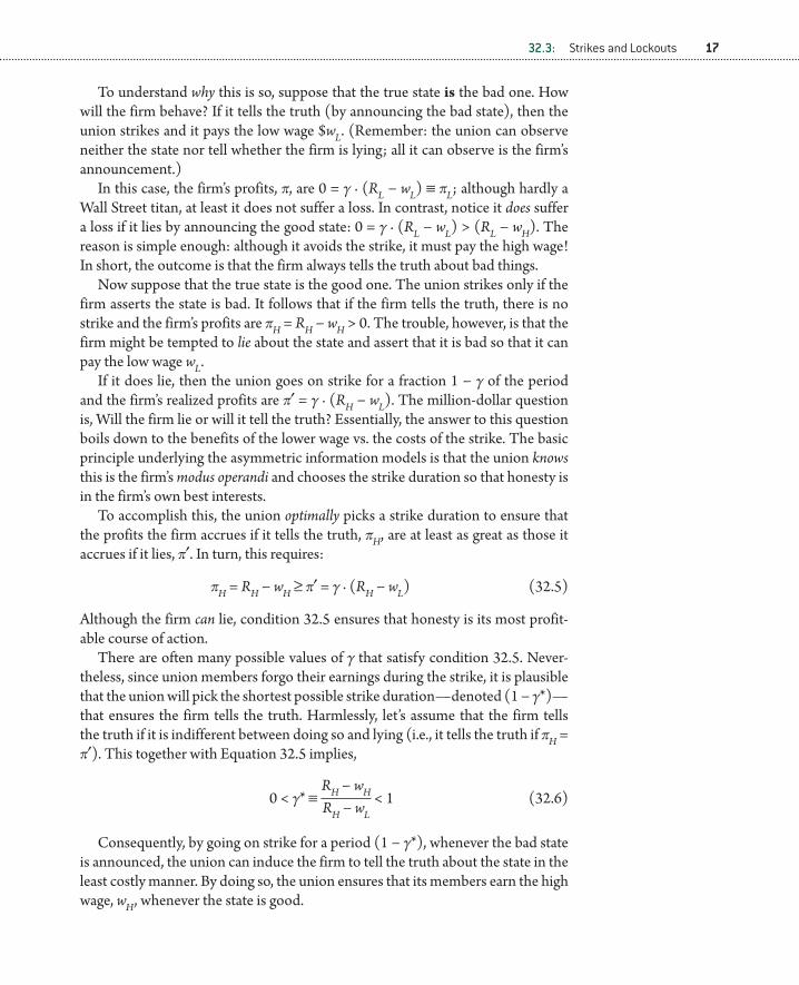
To understand why this is so, suppose that the true state is the bad one. How will the firm behave? If it tells the truth (by announcing the bad state), then the union strikes and it pays the low wage $wL. (Remember: the union can observe neither the state nor tell whether the firm is lying; all it can observe is the firm’s announcement.)
In this case, the firm’s profits, π, are 0 = γ · (RL − wL) ≡ πL; although hardly a Wall Street titan, at least it does not suffer a loss. In contrast, notice it does suffer a loss if it lies by announcing the good state: 0 = γ · (RL − wL) > (RL − wH). The reason is simple enough: although it avoids the strike, it must pay the high wage! In short, the outcome is that the firm always tells the truth about bad things.
Now suppose that the true state is the good one. The union strikes only if the firm asserts the state is bad. It follows that if the firm tells the truth, there is no strike and the firm’s profits are πH = RH − wH > 0. The trouble, however, is that the firm might be tempted to lie about the state and assert that it is bad so that it can pay the low wage wL.
If it does lie, then the union goes on strike for a fraction 1 − γ of the period and the firm’s realized profits are π′ = γ · (RH − wL). The million-dollar question is, Will the firm lie or will it tell the truth? Essentially, the answer to this question boils down to the benefits of the lower wage vs. the costs of the strike. The basic principle underlying the asymmetric information models is that the union knows this is the firm’s modus operandi and chooses the strike duration so that honesty is in the firm’s own best interests.
To accomplish this, the union optimally picks a strike duration to ensure that the profits the firm accrues if it tells the truth, πH, are at least as great as those it accrues if it lies, π′. In turn, this requires:
πH = RH − wH ≥ π′ = γ · (RH − wL) (32.5)
Although the firm can lie, condition 32.5 ensures that honesty is its most profit-able course of action.
There are often many possible values of γ that satisfy condition 32.5. Never-theless, since union members forgo their earnings during the strike, it is plausible that the union will pick the shortest possible strike duration—denoted (1 − γ*)—that ensures the firm tells the truth. Harmlessly, let’s assume that the firm tells the truth if it is indifferent between doing so and lying (i.e., it tells the truth if πH = π′). This together with Equation 32.5 implies,
0 < γ* ≡ RH − wH
RH − wL < 1 (32.6)
Consequently, by going on strike for a period (1 − γ*), whenever the bad state is announced, the union can induce the firm to tell the truth about the state in the least costly manner. By doing so, the union ensures that its members earn the high wage, wH , whenever the state is good.
88147_WEB_ONLY_32_001-040_r2_ra.indd 17 5/17/11 12:00:08 PM

18 Chapter 32: Trade Unions II: Collective Bargaining and Strikes
Be that as it may, an important issue remains to be addressed. Put quite simply, is it all worth it? After all, the union has the option of not going on strike, accept-ing the firm will lie about the good state, and permitting its members to earn wL without the disrupting effects of strikes. Intuitively, the answer to this question depends on both the frequency of strikes required to induce the firm to tell the truth; the duration of the strike, 1 − γ*; and the resulting wage gain, $(wH − wL).
More concretely, with the strike threat, union members earn $wH in the good state and γ* · wL in the bad one (because the union goes on strike). Since the prob-ability of the good state is p and the probability of the bad one is (1 − p), it follows that the expected—or average—earnings of the typical union member are:
average ratings = (1 − p) · γ* · wL + p · wH (32.7)
If the bad state is very unlikely, so p is close to one, then the union is strictly better off using the strike threat. The reason is that, in this case, the threat is rarely carried out and it enables the union to almost always secure the high wage, $wH , as opposed to the low wage, $wL. In contrast, if the bad state is very likely, so that p is close to zero, then the strike threat may not be worthwhile because the union must strike very frequently to force the firm to pay the high wage, $wH , on those rare occasions when the state is actually good.
There are many variants of this basic asymmetric information framework. For example, it can be adapted to explain the incidence of lockouts.32 In this setting, lockouts occur because the firm is unsure about the actual extent of the union’s cohesion under adverse circumstances. Here a lockout represents a rational in-vestment in information by the firm about the union’s cohesion.
Some of the most important recent advances in the area have extended the framework to accommodate a broader set of union sanctions, such as holdouts rather than strikes.33 A holdout means that union members continue to work after their contract expires but under the terms of the original agreement. A holdout can impose substantial costs on the firm. In contrast to a strike, the firm must continue to pay workers. Moreover, the union can lower the firm’s overall produc-tivity by conducting a work-to-rule.
From the perspective of the union’s members, a holdout confers an obvious benefit vis-à-vis a strike because they do not forgo their wages during it. More-over, the firm cannot readily call on outside replacement workers because there is no strike to break. One aspect of a holdout that is especially interesting is that unions can use it as a delay tactic to acquire information about the true state of demand in the industry. More specifically, the union can observe the outcomes of agreements made by other unions and firms in the industry. For example, if the union sees that other similar firms and unions are reaching agreements that call for a very modest wage increase, then it is more liable to believe the claims made by the firm that times are indeed hard.
Other information models—perhaps the most notable being the seminal paper by Ashenfelter and Johnson (1969)—emphasize the informational asymmetries
88147_WEB_ONLY_32_001-040_r2_ra.indd 18 5/17/11 12:00:08 PM
32.3: Strikes and Lockouts 19
that arise within the union itself. The basic idea is that union leaders are interested in seeking reelection but union members seek the best deal possible from the firm and so want a tough leadership. Here wimpy union leaders may call a strike even if they know it has little chance of being effective. The reason is that by doing so they send a signal to their rank and file membership that they are tough. In contrast, if they did not call a strike, then the union membership may suspect that they were sold out by a weak leadership and vote them out of office at the first opportunity.
The Strike ThreatThe strength of the union strike threat is influenced by the legal environment. Some laws prohibit strikes and lockouts altogether. This is particularly so for public unions, where disagreements must be resolved through a process of arbi-tration. Moreover, under the provisions of the 1947 Taft-Hartley Act, the federal government has the authority to call for an 80-day cooling off period, during which time industrial action is illegal. This power was used by President Bush in 2001 to prevent a threatened walkout by Northwest Airline’s mechanics. Other laws circumscribe the actions legally available to unions. For example, the 1959 Landrum- Griffin Act places strict limitations on the actions available to disinter-ested third-party unions. In particular, the law prohibits secondary sympathy ac-tions, which is a serious impediment to both the scope and the effectiveness of the union strike threat.
As for the firm itself, there are a variety of strategies that it can use to reduce the cost of the strike and hence to vitiate the power of the union. One method is for it to accumulate inventories, which it can use to service the demand of its customers during the course of a strike. In this case, the collective action by the union gains traction only after the firm’s inventories are fully depleted. Yet, if the firm pos-sesses a large enough stock of them, this process may take an inordinate amount of time from the perspective of the rank and file union membership who, after all, must make do without a paycheck for the duration of the strike. An alternative tack is for management and the firm’s nonunion employees to keep the plant run-ning while the strike is in progress. An extension of this strategy is for the firm to hire replacement workers.34
In 1981, during the air-traffic controllers strike, then President Reagan used precisely this strategy. His actions sent shock waves through the already delicate strata of U.S. industrial relations that continue to reverberate even to this day. After a summer of strikes initiated by PATCO (the air-traffic controllers union), the president’s patience evidently wore quite thin. Rather than continuing the ne-gotiation process, he fired every member of the union and hired nonunion work-ers in their place. The outcome of this action was that the strike was broken and the union itself was extirpated.35
Clearly, the use of replacement workers reduces the union’s strike threat be-cause the firm can continue to produce output during the dispute (thus lowering
88147_WEB_ONLY_32_001-040_r2_ra.indd 19 5/17/11 12:00:08 PM

20 Chapter 32: Trade Unions II: Collective Bargaining and Strikes
the short-run costs of the strike). Nevertheless, there is evidence that this strat-egy has unpleasant long-run ramifications. In fact, the use of replacement workers may poison the industrial-relation’s climate between the firm and its employees for many years following the conclusion of the strike. Economic Application 32.1 provides evidence of this fatal possibility.
The threat that the firm might use replacement workers implies that the union leadership is less likely to call a strike (lest both they and the union’s members lose their jobs) and is more likely to call for some other form of industrial action—such as a costly holdout.
Nevertheless, if a strike is called, then one implication of the asymmetric infor-mation model is that the use of replacement workers may well increase its dura-tion and hence its severity.36 Recall that the model itself is based on the idea that strikes afford a means whereby the union can induce the firm to tell the truth about the state of business conditions (in particular, the occurrence of the bad state).
In essence, the union keeps the firm honest by punishing it whenever it an-nounces a bad state. However, if the firm can use replacement workers to lower the costs it bears if there is a strike, then ceteris paribus it is less likely that it will tell the truth about the actual state of demand. As a consequence, the union must increase the duration of any strikes it does call for. This may be its only (legal) option for raising the costs of the strike, and inducing the firm to, once again, tell the truth.37
Strikes: The EvidenceKennan and Wilson (1990) articulate the following five stylized facts concerning strike activity in the United States:
1) Strikes are rare. The probability of a strike is about 15 percent, when ne-gotiating a contract to last 3 years. 2) The median strike duration is about 21 days. Although there is an 85 percent chance of settlement before a strike begins, during a strike the probability of settlement is only about 3 percent per day. 3) The settlement probability decreases as the strike goes on. . . . 4) The probability of a strike rises when the economy improves, but strike duration falls. Thus strike incidence is procyclical, but duration is countercy-clical. 5) There is little apparent relationship between strike duration and the terms of settlement.38
Asymmetric information models invoke informational differences between unions and employers to explain strikes and other industrial disputes. The snag is that data which are unavailable to either the union or the firm are almost surely also unavailable to economists in their endeavors to test various hypotheses about union behavior. Fortunately, a number of very useful proxy—or stand in— variables can be observed and hence used as the basis of empirical work.39
88147_WEB_ONLY_32_001-040_r2_ra.indd 20 5/17/11 12:00:08 PM

32.3: Strikes and Lockouts 21
ECOnOMiC AppLiCATiOn 32.1Strikes, Scabs, and Tread SeparationsIn August of 2000, Firestone and Ford jointly announced the recall of over 14 mil-lion tires, many of which were fitted on the Ford Explorer. Subsequently, in Sep-tember of that year, the National Highway Traffic and Safety Administration (NHTSA) issued an advisory concerning several other types of tires produced by Firestone. The NHTSA reported that these tires were under investigation as the cause of 217 fatalities and over 800 injuries. The most common type of failure was a sudden blowout of the tire at high speeds, which was caused by a detach-ment of the rubber tread from the tire’s steel belt. Three of Firestone’s 11 plants—including the Decatur plant in Illinois, which was later identified as responsible for the production of many of the defective tires—previously had been afflicted by a severe strike that began in July 1994.
The strike itself was precipitated by management’s demands for the elimina-tion of the industrywide system of pattern bargaining, a change in the shift sys-tem, and the cutting of pay for new hires by 30%. Almost immediately after the strike began—which involved some 4,200 union members—the firm hired re-placement workers to keep production running.
The private lawsuits and congressional hearings that followed in the aftermath of the highway tragedies generated an exquisite amount of data. As a result, the event has provided economists with an extraordinary portal through which they can closely view the internal workings of the firm and delineate the effects of a deterioration of worker-management relations on product quality.
In an interesting study, Krueger and Mas (2004) collected and used the data generated by the incident to determine what part, if any, the deterioration in worker-management relations at Firestone played in causing the defective tires. The several possible candidate hypotheses that account for the production problems experienced by Firestone can be grouped into two basic categories: those that stress engineering defects and those that stress problems with the labor input.
The hypotheses that stress the failures occurred because of engineering flaws include
Basic design problems in the Ford Explorer and in the tire itself. The use of one or more defective batches of materials. Incorrect instructions were given as to the appropriate tire inflation pressure.
Those that stress the failures occurred because of potential problems with the labor input include
The implementation of a longer shift led to worker fatigue and made workers more prone to errors.
Replacement workers were less skilled than experienced union workers.
88147_WEB_ONLY_32_001-040_r2_ra.indd 21 5/17/11 12:00:08 PM

22 Chapter 32: Trade Unions II: Collective Bargaining and Strikes
Union workers responded to the dispute and the use of replacement workers by reducing their effort.Krueger and Mas (2004) find that tire quality did decline substantially
at those plants that had experienced strikes. Moreover, they present compel-ling evidence that the decline in product quality resulted from the souring of relations between the firm and its employees. In particular, by carefully exam-ining the date of production of tires, they find that productivity declined sub-stantially during the hostile months before the strike commenced and before replacement workers were hired. In addition, product quality declined during the period when many replacement workers and returning strikers worked side by side.
In addition to the tragic fatalities and injuries that occurred, the outcome of the tire fiasco was that the company’s stock value declined by over a half—from $16 billion to $7.5 billion; its top management was either replaced or fired; and the Decatur plant was closed in December 2001. This serves as a salutary reminder indeed, of the critical importance for productive efficiency of the existence of a harmonious relationship between workers and firms. n
A commonly used asymmetric-information proxy is the state of overall de-mand in the economy. During a downturn, it is more likely that the typical firm has experienced a negative demand shock. According to the basic asymmetric information model (in which strikes only occur if the firm announces the state is bad), this implies there will be an increase in strike activity during downturns. Although the evidence is a little more mixed on this, Harrison and Stewart (1994) find that strike duration is countercyclical (i.e., it is longer during recessions than in booms). Similarly, Vroman (1989) finds that the duration of strikes is greater during periods of high unemployment.
Another commonly used proxy is the variability of the stock value of the firm, which reflects increased uncertainty by investors—and presumably unions too—concerning the firm’s true value. An increase in stock price variability is indicative of an increase in the importance of informational asymmetries, which is predicted to increase the incidence of strikes. Tracy (1986, 1987) tests the empirical validity of this hypothesis and confirms it is indeed the case.
Several studies have examined the effects of uncompensated inflation on the in-cidence of strikes. Here the idea is that fluctuations in the inflation rate lead to fluctuations in the value of the real wage. Both Vroman (1989) and Cramton and Tracy (1994a) find that an increase in inflation variability leads to an increase in strike activity. Economic models that emphasize holdouts offer an interesting interpretation of this evidence: a sudden increase in the rate of inflation reduces the real value of the contract wage, which reduces the relative benefits of a holdout vis-à-vis strike. As a result, an increase in inflation is predicted to shift the nature of industrial disputes from holdouts to strikes—a finding that could account for the positive strike-inflation relationship just noted.
88147_WEB_ONLY_32_001-040_r2_ra.indd 22 5/17/11 12:00:08 PM

32.4: Arbitration 23
Finally, a number of papers have attempted to measure the costs of strikes by examining their effects on the firms’ stock market values. DiNardo and Hallock (2002) consider the market’s responses to major strikes that occurred in the pe-riod 1925–1937. They find that strikes had large negative effects on the value of firms, suggesting that they imposed substantial costs on firms. Becker and Olson (1986) have found that a strike involving at least 1,000 workers reduces share-holder wealth by 4.1%.
Although these findings are suggestive of the losses accruing from strike ac-tivity, they may overstate them. The reason is that, according to the asymmetric information model presented earlier, strikes arise because of the privileged infor-mation employers possess concerning the firm’s true value. Moreover, the main prediction of these models is that strikes are most liable to occur when the firm learns that it has experienced a negative shock. In this setting, it is easy to see that a strike can also signal the firm’s bad news to investors, who react accord-ingly. In other words, the observed reduction in the firm’s stock-market valuation could simply reflect the fact that the strike makes investors aware of the firm’s true (lower) value.
32.4 ArbitrationThe inherently messy nature of the praxis of industrial relations implies that, from time to time, disputes will invariably arise between employers and unions. Some of them may stem from grievances over the course of a given contract, such as when the firm is accused of unfairly discharging workers who belong to the union. Other disputes arise when the current contract is due to expire and a new one must be agreed on. As we showed in the last section, sometimes tensions may even escalate to the point where the union calls a strike or the firm stages a lockout.
In many instances, however, strikes and lockouts are simply not a legal option. Instead, if the dispute cannot be resolved peaceably between the two parties, then it must be resolved through the intervention of some neutral third party via a process of arbitration. Arbitration procedures have always been extremely common—indeed mandatory—among public sector unions. However, they are also becoming increasingly so among private-sector unions through the volun-tary agreement of no-strike clauses. These clauses contractually prohibit strikes (and lockouts) during the lifetime of the contract, but allow them once the con-tract expires.40 In exchange for giving up the right to strike, the employer usually compensates the union by agreeing to an assortment of concessions, such as the implementation of elaborate grievance procedures that are triggered if a union member is disciplined or fired.
In the event of a dispute, the resolution process itself can involve several stages. The most basic stage is through mediation. In this process, if the union and firm cannot resolve the dispute themselves, they call on a mediator (whom they both
88147_WEB_ONLY_32_001-040_r2_ra.indd 23 5/17/11 12:00:08 PM

24 Chapter 32: Trade Unions II: Collective Bargaining and Strikes
regard as a disinterested third party). The mediator then proposes various op-tions designed to facilitate a settlement. The union and firm are free to accept or disregard the mediator’s proposals. They can even use them as a basis for further negotiation and then reach an accord of their own choosing.
If the process of mediation is unsuccessful, then the two parties can sometimes call on a neutral third party to initiate a fact-finding mission. The third party col-lects information from both the union and the firm regarding the parameters of the dispute. He or she then crafts a settlement proposal. The proposal may adum-brate the outcome of an arbitration process; however, it is nonbinding so that it can be vetoed by either of the parties involved in the dispute.
The ultimate stage of the dispute resolution process is arbitration. In some instances, the union and firm may agree to arbitration so as to bring about closure to an apparently intractable dispute. In others, however, the two parties are legally bound to settle the dispute via this procedure. In essence, arbitration is akin to the fact-finding process just mentioned—with one crucial difference: the two par-ties are legally obligated to accept the arbitrator’s ruling. While there are a vast num-ber of different possible arbitration arrangements, basically two types are used in practice: conventional arbitration (CA) and final offer arbitration (FOA).41
Both of these mechanisms involve the union and firm (essentially) each writ-ing a separate report that delimits the nature of the dispute (as they see it) and a proposal regarding what they deem to be a fair and reasonable resolution. Under CA the arbitrator looks at both reports, collects data, and interviews the parties involved. The arbitrator then uses the information he or she collects to craft a binding settlement. Under FOA the arbitrator follows the same steps, except that he or she is obliged to choose either the union’s or the firm’s (unamended) settle-ment proposal.
Regardless of the details, the aim of arbitration is to quickly reach a reasonable and effective resolution of the dispute. To accomplish this, it is essential that the firm and the union are provided with the right incentives to truthfully reveal the information that they possess. After all, the arbitrator’s decision can be only as good as the information he or she is given. Consequently, if the union and the firm dissemble and fail to reveal (and misreport) what they know, there is the possibil-ity that the arbitrator may arrive at a very poor decision indeed. The snag is that there are strong grounds for suspecting that the arbitration mechanism provides both the union and the firm with incentives to act strategically against each other, by misrepresenting what they know, so as to influence the arbitrator. The outcome of this horseplay is that arbitration my inadvertently chill the dispute resolution process, rather than promote it. The incentives to truthfully reveal information differ quite markedly between the two arbitration mechanisms just outlined. We begin by discussing the incentives under CA.
Compulsory Arbitration (CA). Suppose that the union and the firm believe that the arbitrator uses a split the difference rule under CA. (Arbitrators may choose
88147_WEB_ONLY_32_001-040_r2_ra.indd 24 5/17/11 12:00:08 PM

32.4: Arbitration 25
this rule because they believe that this rule enhances the chance that they will subsequently be rehired to arbitrate other disputes.) Suppose that the union and the firm are each contemplating proposing a wage of $30 per hour and $20 per hour, respectively. Moreover, suppose that everyone believes that the arbitrator will split the difference and accordingly pick a wage of $25 per hour. It is easy to see that this behavior engenders a powerful incentive for misrepresentation.
For example, if the arbitrator blindly follows the rule, then the union could do better by proposing $40 per hour and even better by proposing $50 (and so on). Likewise, it is in the firm’s best interest to propose the lowest possible wage. The outcome of this process of strategic exaggeration is that the reports produced by the union and the firm may be extremely garbled and as a consequence contain little useful information. As a result of this dissembling behavior, CA may chill rather than promote productive negotiations between the two parties. Moreover, since the information that is provided to the arbitrator is extremely jumbled, he or she may make a very poor quality decision.
Final Offer Arbitration (FOA). Partly in response to the problems just mentioned with CA, Stevens (1966) proposed the idea of final offer arbitration. The idea behind this scheme is that it is supposed to eliminate the gaming that occurs, be-tween the union and the firm, under CA—thus, improving the flow of informa-tion. If this is true, then FOA offers a more productive means of settling disputes. In the simplest setting, the arbitrator looks at the evidence and forms some view as to what he or she regards as an idealized settlement. The resulting incentives for the parties to distort information are quite different from those that arise when using a CA mechanism.
To see this, suppose that the union and the firm are again contemplating pro-posing the wage offers $30 and $20, respectively. Furthermore, suppose that they believe that based on the evidence they have provided, the arbitrator has formu-lated an idealized settlement of (say) $25. In this case, it is in both the union’s and firm’s best interests to make a proposal that is close to $25. Indeed, suppose that the union expects that the firm will propose a wage of $20. In this case, the union could craftily propose $29 (rather than $30). The reason is plain enough to see: the union’s offer will be accepted, since it is closer to the target $25 than is the firm’s offer of $20. Yet the firm is no passive dummy either. Rather, suspecting that this is what the union will do, it could propose a wage of $22. This would clinch the deal. However, the union would then worry that the firm is planning to do this (and so on and so forth). The bottom line is that ultimately both parties converge to the same offer of $25 and truthfully reveal the information they possess to the arbitrator.
While this seems all well and fine on paper, there are some potentially devastat-ing problems that arise in practice. The most acute of them concerns the deter-mination of the arbitrator’s idealized settlement of $25. As observed by Gibbons (1988), this value is not exogenous because of the arbitrator’s own vested interest
88147_WEB_ONLY_32_001-040_r2_ra.indd 25 5/17/11 12:00:08 PM

26 Chapter 32: Trade Unions II: Collective Bargaining and Strikes
in being rehired in the future. Instead, it will be affected by the proposals made by the bargaining parties. Thus although FOA does not induce the arbitrator to follow a simple split the difference rule, it may lead him or her to arrive at a com-promise idealized settlement: one that lies between the union’s and the firm’s two proposals. As a result, the firm and union may, once again, be motivated to act strategically to influence the arbitrator’s idealized settlement. Hence, just as was the case for conventional arbitration, FOA provides incentives for the two parties to misrepresent their information.
32.5 Labor Disputes in professional SportsStrikes, lockouts, and other disputes seemingly are becoming an increasingly prevalent feature of the industrial landscape of the professional sports industry in North America. In their wake they leave millions of distraught fans who vow they will never patronize their beloved sport again. Table 32.1 presents the details of the major strikes (S) and lockouts (L) that have occurred in three major North American professional sports over the last 25 years or so: Major League Baseball (MLB), the National Football League (NFL), and the National Hockey League (NHL).
Economic theory offers valuable insights into the causes of these disputes. In-deed, according to the material presented in Section 32.3, strikes and lockouts are predicted to occur if important informational asymmetries emerge between em-ployers and unions. Lockouts offer a means whereby employers can better ascer-tain the position of the union’s concession curve, and strikes provide unions with a means of assessing the employer’s profitability. On this score, one of the reasons that industrial action is taken with a striking regularity (no pun intended) is that the unique nature of the professional sports industry means that employers have few tools at their disposal to deter strikes, and the costs of a strike (or lockout) appear to be transitory.
Indeed, as we have seen, strikes are more likely to occur (i) the lower the firm’s inventory holdings, (ii) the lower the long-run cost of the strike (to workers and
TABLE 32.1Major Work Stoppages in MLB, the NFL, and NHL
MLB NFL NHL
Industrial Games Industrial Games Industrial Games Year† Event Canceled Year Event Canceled Year Event Canceled
1981 (50) S 712 1982 (57) S 98 1994 (103) L 442
1994–1995 (232) S 920 1987 (24) S 56 2004–2005 L Season†Number in parenthesis refers to the duration of the strike, in days.Source: Schmidt and Berri (2004), table 1, p. 345.
88147_WEB_ONLY_32_001-040_r2_ra.indd 26 5/17/11 12:00:09 PM

32.5: Labor Disputes in Professional Sports 27
the firm), and (iii) the greater the difficulty with which the firm can break a strike by hiring replacement workers.
The basic triumvirate of findings just mentioned bodes very poorly for the fu-ture of the professional sports industry. Employers have no inventories; for ex-ample, it is ridiculous to imagine that the owners of the Dallas Cowboys have a game or two up their sleeves that they can use in the event of an NFL strike. As for the long-run costs of the strike to the league or players’ union, while fans certainly protested they will abandon their beloved sport, they apparently protesteth too much. Schmidt and Berri (2004) find that none of the sports stoppages reported in Table 32.1 had any discernable permanent effect on attendance. (Similar find-ings are reported in Schmidt and Berri (2002), who focus exclusively on MLB.) Finally, although the owners could presumably hire replacement workers, this can hardly be viewed as a credible option. After all, fans want to see their favorite athletes compete rather than a few hams picked more or less randomly off the streets.
As for the economic impact of strikes and lockouts on the local economies of those cities that host a professional sports team, Coates and Humphreys (2001) find, using data from the National Basketball Association (NBA), they are— contrary to commonly made claims—very small. The authors conjecture that this is because, during the strike, fans substitute toward other activities that are available in the city.
Of course, not all disputes end with a strike or lockout, and in many instances the league and the players’ union attempt to reach a settlement via arbitration. Economic Application 32.2 examines how final offer arbitration (FOA) is used in MLB to resolve contractual difficulties.
ECOnOMiC AppLiCATiOn 32.2Final Offer Arbitration: The Case of Major League BaseballThe salaries of Major League players are determined in the following manner. First, professional league players are bound to their club for a period of 6 years. Second, for the first 3 years of their contract, their bargaining is limited in scope to negotiating exclusively with their own team, under more or less monop-sonistic conditions. Third, after 6 years have elapsed they become free agents and can sell their labor services to the highest bidder. The result of free agency is usually a pronounced increase in players’ earnings. Finally, during the initial 3- to 6-year window, although they are bound to their club, they may unilaterally adopt to have their salary determined through FOA. If they do so, then the arbitra-tor must determine the appropriate wage for the player, and his or her decision is final.
In trying to influence the arbitrator’s position, the team has an incentive to emphasize the low monopsonistic wage. For their part, players have every incen-tive to stress the stellar earnings available to them under free agency. The basic
88147_WEB_ONLY_32_001-040_r2_ra.indd 27 5/17/11 12:00:09 PM

28 Chapter 32: Trade Unions II: Collective Bargaining and Strikes
theoretical prediction is that the arbitrator’s preferred position reflects a compro-mise between these two viewpoints.
Marburger (2004) tests this hypothesis using Major League Baseball FOA of-fers over the period 1986–2002. His main finding is that there is strong evidence that final offers are indeed strategically formulated around the preferred award. Moreover, the preferred award is itself a weighted average of the player’s salary in the previous season and the average free agent salary.
More broadly, these findings suggest that great care must be exercised in de-signing robust arbitration schemes. More specifically, although FOA was de-signed to eliminate the dissembling of information that arises under CA (because of arbitrator compromise), it may remain a potent force under FOA. n
Summary Economists have formulated several alterna-
tive models for understanding the nature of the collective bargaining agreements reached between employers and unions.
Under the monopoly union model, the union picks the wage and the firm responds by se-lecting its profit maximizing level of employ-ment. The outcome is unique, and the level of employment is inefficiently low.
The efficient contract curve is the locus of indi-vidually rational wage-employment contracts that obtain at the points of tangency between the union’s indifference curves and the firm’s isoprofit curves. All of the points on the con-tract curve lie to the right of the labor-demand curve.
Strongly efficient contracts are agreements that fully exploit all economic opportunities, in-cluding those available to union workers from employment with alternative employers. The strongly efficient contract curve is vertical (in wage-employment space), and passes through the competitive level of employment.
Both the efficient and strongly efficient con-tract curves include an infinite number of possible wage-employment combinations. Bar-gaining theory sheds light on which of the many possible outcomes will materialize.
Strikes are relatively rare. Modern economics views them as an investment in information that permits the union to gather valuable infor-mation about the firm’s true state of demand.
ProblemSp1. What are the principal differences between the monopoly union, efficient contracting, and strongly efficient contracting approaches?
p2. The MRP is MRP = 100 − 2 · L and the union’s utility is U = w · L. What is the outcome predicted by the monopoly union model?
p3. The MRP is $MRP = 100 − 2 · L and the com petitive wage is wc = $30. Suppose that the firm and the union have negotiated the efficient contract $w = 40 and L = 40. How much would they jointly gain by instead choosing a strongly efficient contract?
88147_WEB_ONLY_32_001-040_r2_ra.indd 28 5/17/11 12:00:09 PM

Notes 29
Hint: The area under the MRP schedule between any two levels of employment L1 > L0 equals (L1 − L0 ) · (100 + L0 − L1).
p4. Are strikes irrational?
p5. Let τ denote the duration of the strike, in years. Assume that the employer’s concession curve, CC, is $w = 2 · exp [τ] and that the union’s resistance curve (RR) is $w = 4 · exp [− τ]. A union leader puts an offer of $3 to the firm. Does a strike ensue? If so, how long does it last and what is the final wage offer?
Now suppose that just before the negotiations, Congress passed a law that allowed striking union members to receive welfare benefits and that, as a result, the union’s resistance curve shifted to $w = 8 · exp [− τ]. What explains this shift, and what happens to the length of a strike, if one occurs?
Hint: ln 2 ≈ 0.69.
p6. Consider a situation in which an employer is better informed about the true state of demand than is the union. The facts are as follows: There are two states good (g) and bad (b), and the probability of the good state is p; the firm’s revenues (per worker) are $Rg = 110 in the good state and $Rb = $30 in the
bad one; and the wage agreement is wg = $90 if the firm announces the good state, and it is wb = $30 if it announces the bad one.
(a) Suppose that the firm and the union agreed to a no-strike clause. What is the outcome in this environ-ment (in particular: What is the wage that pertains in each state? What are the firm’s expected profits? What are the expected earnings of the typical union member?)
(b) Now suppose that if the firm announces the bad state (i.e., business conditions are bad) the union works for only a fraction γ of the period and strikes for the remaining (1 − γ).
(c) Can the union use the strike threat to induce honesty on the part of the firm about the true state of business conditions? What is the shortest strike dura-tion that will accomplish this goal?
(d) If the probability of the good state is p = 0.1, does the union gain from the strike threat?
p7. What are the principal economic reasons for the rocky industrial relations witnessed in the profes-sional sports industry?
NoteS 1. I appreciate comments from Peter Crampton and
Joel Tracy that led to substantial improvements in this chapter. Naturally, I’m responsible for any re-maining deficiencies.
2. Section 32.3 considers the case in which bargain-ing reaches an impasse, leading to a strike or a lockout.
3. See http://library.albany.edu/speccoll/document inglabor/bargaining.htm (accessed May 5, 2010).
4. Some elements of the employment relationship are so complicated that they cannot be written down in a formal legal language—legalese. In this case, the union and the firm might arrive at an implicit understanding of what constitutes reason-able behavior.
5. Samuel Gompers (1850–1924) was the first presi-dent of the American Federation of Labor (AFL). His reply is often cynically shortened to “more.”
6. Understanding the potential conflicts of interest that arise between unions and their members is a very difficult problem; Cai (2000) has made im-portant progress along this dimension.
7. Farber and Saks (1980) show how union prefer-ences can be derived from the preferences of in-dividual union members. They apply their model to understand the bargaining objectives of the United Mine Workers (UMW). See also Farber (1986). Dunlop (1944) was one of the first stud-ies in this area. He suggested that unions are in-terested in maximizing the wage bill, implying that U = w · L.
88147_WEB_ONLY_32_001-040_r2_ra.indd 29 5/17/11 12:00:09 PM

30 Chapter 32: Trade Unions II: Collective Bargaining and Strikes
8. The convexity of each indifference curve stems from the assumed diminishing marginal utility of individual consumption.
9. Recall that in a competitive environment, MRPL = p · MPL, where MPL is the marginal product of labor.
10. Oswald (1982) offers a detailed analysis of this model. Notice that, according to assumption 32.1a, the union sets a unique wage, w. In more complicated models, the union is viewed as a discriminating monopolist and can set many dif-ferent wages. See, for example, Frank (1985) and Kuhn (1988).
11. McDonald and Solow (1981) formalized the efficient-contracting model.
12. That is, a contract is efficient if and only if it lies on the contract curve.
13. See Johnson (1990) who not only discusses feath-erbedding in general but also studies the bargain-ing process that leads to the incorporation of these rules into union contracts in particular.
14. According to Definition 32.1, the criterion used to judge whether an outcome is efficient depends on having the correct measures of employer and union well-being.
15. Recall that union members care only about their consumption and not where they work.
16. To see this, notice that those who are retained continue to earn $w0. Those who are laid off earn the competitive wage, $wc , and they receive the severance payment s0. It follows from the defini-tion of s0 that their income is wc + s0 = w0 , which is identical to their predisplacement incomes.
17. Notice that the firm (and union) always want to set L = Lc. Any other choice leaves unexploited opportunities for raising the firm’s profits, like those depicted in region II.
18. Under MH the union already has all of the bar-gaining power, so it cannot increase any further. Under EH and SH an increase in bargaining power leads to a movement along the pertinent contract curve.
19. Clark (1984) and Voos and Mishel (1986) study the broader effects of unions on profits.
20. For example, see Pencavel (1984), MaCurdy and Pencavel (1986), Brown and Ashenfelter (1986), Eberts and Stone (1986), Card (1986), Christo-fides and Oswald (1992), Hendricks and Kahn (1991), and Wessels (1991).
21. See, for example, Abowd (1989).
22. As Gu and Kuhn (1998) report, holdouts—that is, the continuation of negotiations beyond the contract expiry date—are far more common.
23. In what follows, we focus on strikes. The same basic arguments, however, hold for lockouts, in which case it is the firm that strikes the union.
24. Hicks (1966; first published in 1932).
25. Schnell and Gramm (1987) test whether bargain-ing units learn from their mistakes by investigating whether strike experience has a negative— teetotaler—effect on a union’s future strike procliv-ities. Using a large data set, they find that the expe-rience of a strike is sobering. A union’s future strike incidence declines by about 50% after a strike.
26. Coles and Hildreth (2000) provide a formal model that examines the strategic role played by inventories in the bargaining process. In Great Britain, before the passage of the 1982 Employ-ment Act, union truculence prevented firms from moving their inventories across picket lines during a strike. However, the act removed these impedi-ments. The authors present evidence indicating that the passage of the act led to a relative decline in the union wage.
27. There are many papers devoted to understanding the role of informational asymmetries. Ashen-felter and Johnson (1969) is one of the earliest. This section draws from the excellent surveys by Kennan (1986), Card (1990), and Kennan and Wilson (1993).
28. Indeed, this position was articulated by Hicks (1966, pp. 146–147) himself, “The strike arises from the divergence of estimates, . . . the . . . ignorance by one side of the others dispositions.”
88147_WEB_ONLY_32_001-040_r2_ra.indd 30 5/17/11 12:00:09 PM
29. Kennan and Wilson (1993), p. 46.
30. For instance, the firm’s management may learn the good news that a customer is planning to place a multimillion-dollar order next year. Alternatively, it could learn the bad news that an existing large customer intends to switch to a different firm.
31. The model is a simplified version of the one pre-sented in Forsythe, Kennan, and Sopher (1991).
32. Important recent work emphasizes the ability of unions to undertake other forms of industrial ac-tion, such as holdouts. During a holdout, individ-ual union members continue to work after their contract expires, but with less zest and diligence. See for example, Cramton and Tracy (1994a, 1994b) and Gu and Kuhn (1998).
33. See Cramton and Tracy (1994a, 1994b, 2003) and Gu and Kuhn (1998).
34. The use by employers of replacement workers is nothing new in the United States. Rosenbloom (1998) examines the role of strikebreakers using data from over 2,000 separate strikes that occurred between 1881 and 1894.
35. Cramton and Tracy (1998) estimate that the in-creased use of replacement workers, since the early 1980s, has significantly reduced the number of strikes.
36. Cramton and Tracy (1998) find that the in-creased willingness of employers to use replace-ment workers during a strike has led to a switch in union tactics. They report that while the number of strikes decreased by about 50% between 1970 and 1996, the number of holdouts almost tripled. They also find that the use of replacement workers leads to a greater number of disputes.
37. Schnell and Gramm (1994) analyze strike data between 1985 and 1989. They find that employ-ers’ use of replacement workers during a strike is associated with longer strikes than otherwise would have occurred.
38. Kennan and Wilson (1990), p. 406.
39. The following discussion draws from Cramton and Tracy (2003).
40. These agreements are particularly common in sit-uations in which time is of the essence, such as in construction projects, and even among unionized teaching assistants.
41. A number of papers have explored the economics of arbitration. See, for example, Ashenfelter and Bloom (1984), Ashenfelter and Hyslop (2001), Bloom and Cavanagh (1986), Crawford (1981), Currie (1994) and Farber (1981).
42. In this section, we consider only strongly efficient contracts. The arguments presented here apply with equal force to efficient contracts that lie on the contract curve XY.
43. John Nash (of A Beautiful Mind fame) was awarded the Nobel Prize in economics in 1994 for his pio-neering work in game theory.
44. An alternative and equally valid approach is to as-sume that the firm hires less qualified replacement workers, in which case πa equals its profits from doing so.
45. In a similar ilk, no (sane) person would write her-self a check for a million dollars and claim she was wealthy.
46. Svejnar (1986) offers econometric evidence on the economic forces that determine precisely where along the contract curve XY the union and firm reach an agreement. He finds that, although there is considerable dispersion, several of the union-firm units he looks at have 50% bargaining weight. His results also provide limited support for the presence of strongly efficient contracts. See also Doiron (1992).
47. The exposition follows that given in Sutton (1986).
48. Groundhog Day is a (1993) film starring Bill Murray. In it he visits Punxsutawney, Pennsylva-nia, and is caught in a time warp, where he lives the same day over and over again.
Notes 31
88147_WEB_ONLY_32_001-040_r2_ra.indd 31 5/17/11 12:00:09 PM

32 Chapter 32: Trade Unions II: Collective Bargaining and Strikes
refereNceSAbowd, John M. (1989). “The Effect of Wage Bargains
on the Stock Market Value of the Firm.” American Economic Review 79(4): 774–800.
Ashenfelter, Orley, and David E. Bloom. (1984). “Models of Arbitrator Behavior: Theory and Evi-dence.” American Economic Review 74(1): 111–124.
Ashenfelter, Orley, and Dean Hyslop. (2001). “Mea-suring the Effect of Arbitration on Wage Levels: The Case of Police Officers.” Industrial and Labor Relations Review 54(2): 316–328.
Ashenfelter, Orley, and George E. Johnson. (1969). “Bargaining Theory, Trade Unions, and Industrial Strike Activity.” American Economic Review 59(1): 35–49.
Becker, Brian E., and Craig A. Olson. (1986). “The Impact of Strikes on Shareholder Equity.” Industrial and Labor Relations Review 39(3): 425–438.
Bloom, David E., and Christopher L. Cavanagh. (1986). “An Analysis of the Selection of Arbitrators.” American Economic Review 76(3): 408–422.
Brown, James N., and Orley Ashenfelter. (1986). “Testing the Efficiency of Employment Contracts.” Journal of Political Economy 94(3): S40–S87.
Cai, Hongbin. (2000). “Bargaining on Behalf of a Constituency.” Journal of Economic Theory 92(2): 234–273.
Card, David. (1986). “Efficient Contracts with Costly Adjustment: Short-run Employment Determination for Airline Mechanics.” American Economic Review 76(5): 1045–1071.
———. (1990). “Strikes and Bargaining: A Survey of the Recent Empirical Literature.” American Economic Review 80(2): 410–415.
Christofides, Louis N., and Andrew J. Oswald. (1992). “Real Wage Determination and Rent-Sharing in Collective Bargaining Agreements.” Quarterly Journal of Economics 107(3): 985–1002.
Clark, Kim B. (1984). “Unionization and Firm Perfor-mance: The Impact on Profits, Growth, and Produc-tivity.” American Economic Review 74(5): 893–919.
Coates, Dennis, and Brad R. Humphreys. (2001). “The Economic Consequences of Professional Sports Strikes and Lockouts.” Southern Economic Journal 67(3): 737–747.
Coles, Melvyn, and Andrew K. Hildreth. (2000). “Wage Bargaining, Inventories, and Union Legisla-tion.” Review of Economic Studies 67(2): 273–293.
Cramton, Peter C., and Joseph S. Tracy. (1994a). “The Determinants of U.S. Labor Disputes.” Journal of Labor Economics 12(2): 180–209.
———. (1994b). “Wage Bargaining with Time-Varying Threats.” Journal of Labor Economics 12(4): 594–617.
———. (1998). “The Use of Replacement Workers in Union Contract Negotiations: The U.S. Experience, 1980–1989.” Journal of Labor Economics 16(4): 667–701.
———. (2003). “Unions, Bargaining and Strikes.” In International Handbook of Trade Unions. Ed. John T. Addison and Claus Schnabel. Cheltenham, UK: Edgar Allen.
Crawford, Vincent P. (1981). “Arbitration and Conflict Resolution in Labor-Management Bargaining.” American Economic Review 71(2): 205–210.
Currie, Janet. (1994). “Arbitrator Behavior and the Variances of Arbitrated and Negotiated Wage Settle-ments.” Journal of Labor Economics 12(1): 29–40.
DiNardo, John, and Kevin F. Hallock. (2002). “When Unions ʻMattered’: The Impact of Strikes on Fi-nancial Markets, 1925–1937.” Industrial and Labor Relations Review 55(2): 219–233.
Doiron, Denise J. (1992). “Bargaining Power and Wage-Employment Contracts in a Unionized Indus-try.” International Economic Review 33(3): 583–606.
Dunlop, John T. (1944). Wage Determination Under Trade Unions. New York: MacMillan.
Eberts, Randall W., and Joe A. Stone. (1986). “On the Contract Curve: A Test of Alternative Models of Collective Bargaining.” Journal of Labor Economics 4(1): 66–81.
88147_WEB_ONLY_32_001-040_r2_ra.indd 32 5/17/11 12:00:10 PM

Farber, Henry S. (1981). “Splitting-the-Difference in Interest Arbitration.” Industrial and Labor Relations Review 35(1): 70–77.
———. (1986). “The Analysis of Union Behavior.” In Handbook of Labor Economics. Vol. 2. Ed. Orley Ashenfelter and Richard Layard. Amsterdam, North Holland: Elsevier, pp. 1039–1089.
Farber, Henry S., and Daniel H. Saks. (1980). “Why Workers Want Unions: The Role of Relative Wages and Job Characteristics.” Journal of Political Economy 88(2): 349–369.
Forsythe, Robert, John Kennan, and Barry Sopher. (1991). “An Experimental Analysis of Strikes in Bargaining Games with One-Sided Private Informa-tion.” American Economic Review 81(1): 253–278.
Frank, Jeff. (1985). “Trade Union Efficiency and Over-employment with Seniority Wage Scales.” Economic Journal 95(380): 1021–1034.
Gibbons, Robert. (1988). “Learning In Equilibrium Models of Arbitration.” American Economic Review 78(5): 896–912.
Gu, Wulong, and Peter Kuhn. (1998). “A Theory of Holdouts in Wage Bargaining.” American Economic Review 88(3): 428–449.
Harrison, Alan, and Mark Stewart. (1994). “Is Strike Behavior Cyclical?” Journal of Labor Economics 12(4): 524–553.
Hendricks, Wallace E., and Lawrence M. Kahn. (1991). “Efficiency Wages, Monopoly Unions and Efficient Bargaining.” Economic Journal 101(408): 1149–1162.
Hicks, John R. (1966). The Theory of Wages. 2nd ed. New York: St. Martin’s Press.
Johnson, George E. (1990). “Work Rules, Feather-bedding, and Pareto-optimal Union-Management Bargaining.” Journal of Labor Economics 8(1): S237–S259.
Kennan, John. (1986). “The Economics of Strikes.” In Handbook of Labor Economics. Vol. 2. Ed. Orley Ashenfelter and Richard Layard. Amsterdam, North Holland: Elsevier, pp. 1091–1137.
Kennan, John, and Robert Wilson. (1990). “Can Strategic Bargaining Models Explain Collective Bargaining Data?” American Economic Review 80(2): 405–409.
———. (1993). “Bargaining with Private Information.” Journal of Economic Literature 31(1): 45–104.
Krueger, Alan B., and Alexandre Mas. (2004). “Strikes, Scabs, and Tread Separations: Labor Strife and the Production of Defective Bridgestone/Firestone Tires.” Journal of Political Economy 112(2): 253–289.
Kuhn, Peter. (1988). “A Nonuniform Pricing Model of Union Wages and Employment.” Journal of Political Economy 96(3): 473–508.
MaCurdy, Thomas E., and John H. Pencavel. (1986). “Testing between Competing Models of Wage and Employment Determination in Unionized Markets.” Journal of Political Economy 94(3, Part 2): S3–S39.
Marburger, Daniel R. (2004). “Arbitrator Compromise in Final Offer Arbitration: Evidence from Major League Baseball.” Economic Inquiry 42(1): 60–68.
McDonald, Ian M., and Robert M. Solow. (1981). “Wage Bargaining and Employment.” American Economic Review 71(5): 896–908.
Nash, John Jr. (1950). “The Bargaining Problem.” Econometrica 18(1): 155–162.
Oswald, Andrew J. (1982). “The Microeconomic Theory of the Trade Union.” Economic Journal 92(367): 576–595.
Pencavel, John H. (1984). “The Tradeoff be-tween Wages and Employment in Trade Union Objectives.” Quarterly Journal of Economics 99(2): 215–231.
Rosenbloom, Joshua L. (1998). “Strikebreaking and the Labor Market in the United States, 1881–1894.” Journal of Economic History 58(1): 183–205.
Rubinstein, Ariel. (1982). “Perfect Equilibrium in a Bargaining Model.” Econometrica 50(1): 97–109.
———. (2002). “The Impact of the 1981 and 1994–1995 Strikes on Major League Baseball Attendance: A Time-Series Analysis.” Applied Economics 34(4): 471–478.
References 33
88147_WEB_ONLY_32_001-040_r2_ra.indd 33 5/17/11 12:00:10 PM

34 Chapter 32: Trade Unions II: Collective Bargaining and Strikes
Schmidt, Martin B., and David J. Berri. (2004). “The Impact of Labor Strikes on Consumer Demand: An Application to Professional Sports.” American Economic Review 94(1): 344–357.
Schnell, John F., and Cynthia L. Gramm. (1987). “Learning by Striking: Estimates of the Teetotaler Effect.” Journal of Labor Economics 5(2): 221–241.
———. (1994). “The Empirical Relations between Employers’ Striker Replacement Strategies and Strike Duration.” Industrial and Labor Relations Review 47(2): 189–206.
Stevens, C. M. (1966). “Is Compulsory Arbitration Compatible with Bargaining?” Industrial Relations 5(1): 38–50.
Sutton, John. (1986). “Non-Cooperative Bargain-ing Theory: An Introduction.” Review of Economic Studies 53(5): 709–724.
Svejnar, Jan. (1986). “Bargaining Power, Fear of Disagreement, and Wage Settlements: Theory
and Empirical Evidence from U.S. Industry.” Econometrica 54(5): 1055–1078.
Tracy, Joseph S. (1986). “An Investigation into the Determinants of U.S. Strike Activity.” American Economic Review 76(3): 423–436.
———. (1987). “An Empirical Test of an Asymmet-ric Information Model of Strikes.” Journal of Labor Economics 5(2): 149–173.
Voos, Paula B., and Lawrence R. Mishel. (1986). “The Union Impact on Profits: Evidence from Industry Price-Cost Margin Data.” Journal of Labor Economics 4(1): 105–133.
Vroman, Susan B. (1989). “A Longitudinal Analysis of Strike Activity in U.S. Manufacturing: 1957–1984.” American Economic Review 79(4): 816–826.
Wessels, Walter J. (1991). “Do Unions Contract for Added Employment?,” Industrial and Labor Relations Review 45(1): 181–193.
88147_WEB_ONLY_32_001-040_r2_ra.indd 34 5/17/11 12:00:10 PM
Appendix 32.A: Collective Bargaining Agreements 35
Appendix 32.A Collective Bargaining AgreementsIn the text, we characterized the set of strongly efficient contracts as points that lie along the contract curve (line) CS shown in Figure 32.6.42 It is fair to say, however, that as things currently stand, we have only scotched the snake, not killed it. The reason is that there are many—indeed an infinite number—of these contracts that lie along the CS locus.
Of course, economists ideally would like to determine which of the many pos-sible contracts is the one that is actually agreed on between the union and the firm. Only then can they predict, for example, the wage and employment levels that arise from collective bargaining and relate them to other variables of eco-nomic interest.
It is useful to think of movements along the contract curve CS as a tug of war between the union and the firm. The union wants to pull the final agreement as close as possible to point S; for its part, the firm wants to pull it as close as pos-sible to point C. For a long time, economists argued that the actual outcome is indeterminate, depending on the relative bargaining power of both parties. Yet, since economists were somewhat clueless regarding the difficult problem of how to model this, an impasse resulted: it was impossible to predict the specific con-tractual agreement with any degree of confidence.
Over the years, however, revolutionary advances have taken place in bargain-ing theory. Economists now possess the tools that enable them to model and hence crystallize the relatively elusive concept of bargaining power itself. The first ma-jor advance came with the publication of John Nash’s (1955) paper, which laid the foundations of what is known as cooperative bargaining theory.43 The second, with the publication of Ariel Rubinstein’s (1982) seminal paper, laid the foun-dations of noncooperative bargaining theory. The key difference between the two approaches is that cooperative bargaining theory suppresses details con-cerning the bargaining process itself and, instead, proposes conditions that any reasonable bargaining agreement must satisfy. In contrast, noncooperative bar-gaining theory imposes fewer restrictions on the bargaining agreement, but goes to great lengths to specify the procedures the parties follow during their negotiations. The differences between the two approaches are best understood by seeing them in action.
The nash Bargaining Solution. Consider a union and a firm that are bargain-ing over which strongly efficient contract is acceptable to them. Model 32.2, de-scribes the details.
Part (a) of Model 32.2 reasserts the focus on strongly efficient contracts. Al-though the assumption that Lc ≡ 1 is designed to simplify the arithmetic, it might at first sight seem a little mysterious. It does not mean that the firm hires only one worker. Instead, it means that the firm hires one labor unit. These sorts of normalizations occur all the time. For example, the reader probably already says,
88147_WEB_ONLY_32_001-040_r2_ra.indd 35 5/17/11 12:00:10 PM
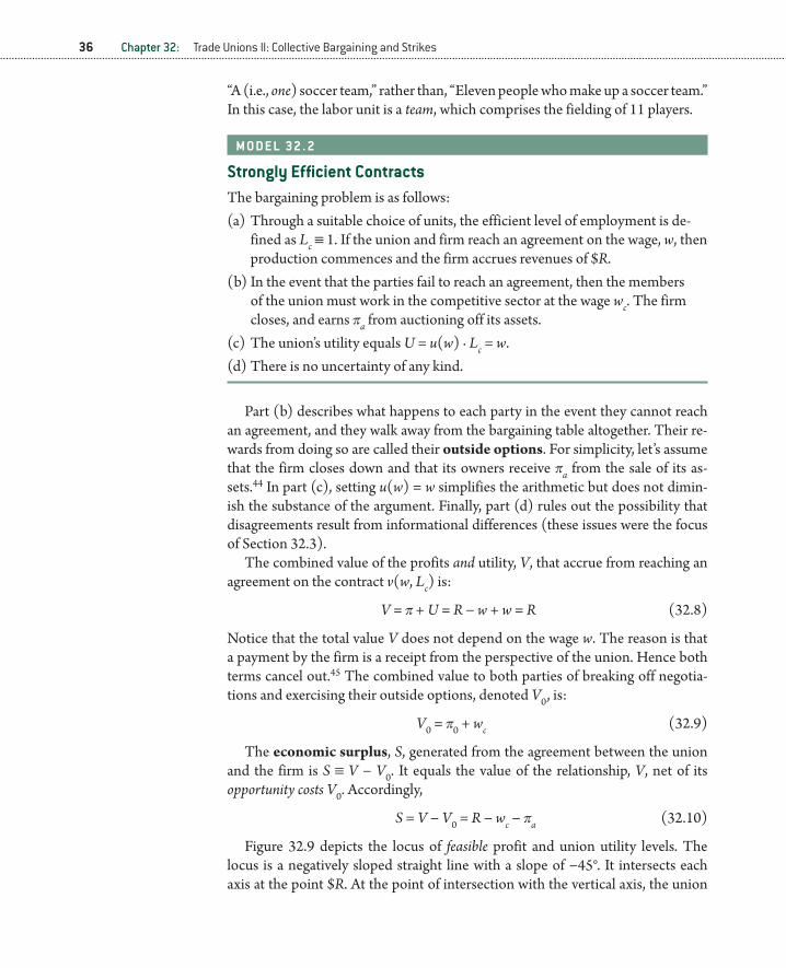
36 Chapter 32: Trade Unions II: Collective Bargaining and Strikes
“A (i.e., one) soccer team,” rather than, “Eleven people who make up a soccer team.” In this case, the labor unit is a team, which comprises the fielding of 11 players.
M O D E L 32 . 2
Strongly Efficient ContractsThe bargaining problem is as follows:(a) Through a suitable choice of units, the efficient level of employment is de-
fined as Lc ≡ 1. If the union and firm reach an agreement on the wage, w, then production commences and the firm accrues revenues of $R.
(b) In the event that the parties fail to reach an agreement, then the members of the union must work in the competitive sector at the wage wc. The firm closes, and earns πa from auctioning off its assets.
(c) The union’s utility equals U = u(w) · Lc = w.(d) There is no uncertainty of any kind.
Part (b) describes what happens to each party in the event they cannot reach an agreement, and they walk away from the bargaining table altogether. Their re-wards from doing so are called their outside options. For simplicity, let’s assume that the firm closes down and that its owners receive πa from the sale of its as-sets.44 In part (c), setting u(w) = w simplifies the arithmetic but does not dimin-ish the substance of the argument. Finally, part (d) rules out the possibility that disagreements result from informational differences (these issues were the focus of Section 32.3).
The combined value of the profits and utility, V, that accrue from reaching an agreement on the contract v(w, Lc) is:
V = π + U = R − w + w = R (32.8)
Notice that the total value V does not depend on the wage w. The reason is that a payment by the firm is a receipt from the perspective of the union. Hence both terms cancel out.45 The combined value to both parties of breaking off negotia-tions and exercising their outside options, denoted V0 , is:
V0 = π0 + wc (32.9)
The economic surplus, S, generated from the agreement between the union and the firm is S ≡ V − V0. It equals the value of the relationship, V, net of its opportunity costs V0. Accordingly,
S = V − V0 = R − wc − πa (32.10)
Figure 32.9 depicts the locus of feasible profit and union utility levels. The locus is a negatively sloped straight line with a slope of −45°. It intersects each axis at the point $R. At the point of intersection with the vertical axis, the union
88147_WEB_ONLY_32_001-040_r2_ra.indd 36 5/17/11 12:00:10 PM

Appendix 32.A: Collective Bargaining Agreements 37
accrues all of the revenues generated by the firm and divides them equally among all of its members.
Although points that lie inside the fron-tier are feasible, they are inefficient. The rea-son is that given any such point (such as A), then both parties can be made better off by moving onto the frontier itself.
Rather than reaching an agreement, both parties always have the option of walking away and exercising their outside options. In the figure, their outside options are depicted at point B. Since neither the union nor the firm would rationally agree to a deal that makes them worse off than their respective outside options, then the set of agreements that are individually rational for both the union and the firm lie both on and inside the shaded triangle BCD. Of these points, only those that lie on the frontier CD are both ra-tional and efficient.
The goal of an efficient bargain is to move the parties from the status quo point B to some point on the frontier CD. How is this to be done? According to the Nash bargaining solution, it is accomplished in the following way. The parties each get their outside options plus a given fraction of the surplus, S. More specifically, let 0 ≤ β ≤ 1 denote the fraction of the surplus that goes to the union and the remaining fraction 1 − β that goes to the firm. For instance, β = 1
2 corre-sponds to a 50–50 split. Thus, according to the Nash bargain, the wage agreement (denoted $w*) is given by:
w* = wc + β · S = wc + β · (R − wc − πa ) (32.11)
Rearranging this expression and solving for the wage, w* gives:
w* = wc · (1 − β) + β · (R − πa ) (32.12)
From this it is easy to see that β does indeed capture the union’s bargaining power. Notice that if β = 1, then the union has all of the bargaining power. In this case w* = (R − πa), indicating that the union membership captures all of the firm’s rents R − πa (this corresponds to point C in the figure). In contrast, if β = 0, then the union has none of the bargaining power. In this case, the firm is able to drive the wage down to w* = wc—which is the same as each union member’s outside option (see point D).46 Point E in the figure corresponds to the case in which β = 12 , which represents a 50–50 split of the surplus S. Notice that for this value of β, the agree-ment point E is located at the midpoint of the efficient bargaining locus CE.
A
B
C
D
E
πa π*
Symmetricbargain: β = ½
Individually rationalagreements
πProfits
$w
wc
w*
R
REfficient bargains
FigUrE 32.9 The Bargaining Frontier
88147_WEB_ONLY_32_001-040_r2_ra.indd 37 5/17/11 12:00:11 PM

38 Chapter 32: Trade Unions II: Collective Bargaining and Strikes
The model generates several interesting predictions regarding the properties of the wage agreement $w*. In particular, an increase in the firm’s rents, measured by R − πa raises the wage. This is consistent with the finding that unions form—and union wages are greatest—in highly concentrated industries (such as in the steel industry) where industry rents are the greatest. Finally, an increase in the alter-native (competitive) wage $wc is predicted to raise the union wage. This finding has an interesting implication for the effects of changes in the minimum wage. To see why, suppose that the alternative wage, $wc , equals the federal minimum wage. Given this, it is easy to see why unions lobby so forcefully to increase it: by doing so they increase their own wage $w*.
The rubinstein Bargaining ModelPatience is bitter, but its fruit is sweet.
—Phaedrus
There can be little doubt that the Rubinstein (1982) bargaining model represents one of the most significant advances in economic theory over the past 50 years or so. It enjoys myriad applications in economics in general and labor economics in particular. Although a formal analysis of the model is somewhat technical and daunting, it is possible to go far with little. Consequently, the aim of this section is to spell out the essentials of the approach. Model 32.3 describes the basic bargain-ing problem.47 The application to the trade unions follows.
Part (a) of Model 32.3 describes the essence of the bargaining problem and part (b) the means whereby an agreement is reached.
M O D E L 32 . 3
The rubinstein Bargaining ModelThe bargaining game is as follows:(a) Two individuals, Dougal (D) and Betsy (B), must agree on how to split a
cake. Let s denote Dougal’s share and 1 − s Betsy’s.(b) Every period, one of them gets to make a proposal regarding the division of
the cake. The other can respond by saying yes (Y) or no (N) to the offer. If yes, then the negotiations stop, and they divide and consume the cake. If no, then the negotiations continue.
(c) The negotiation process is one in which each of them gets to make an offer in turn. Dougal gets to make the first offer at date t = 0.
(d) Both Dougal and Betsy are equally impatient, preferring cake today rather than cake tomorrow. Indeed, each of them values receiving a share, s, of the cake next period at only δ · s, where δ < 1.
88147_WEB_ONLY_32_001-040_r2_ra.indd 38 5/17/11 12:00:11 PM

Appendix 32.A: Collective Bargaining Agreements 39
Assumption (c) can be relaxed in a variety of ways. For example, at each stage Dougal and Betsy could toss a coin to see who gets to make the offer. The assump-tion is that δ < 1 puts fire under their feet to quickly reach an agreement. Notice that for very small values of δ, close to zero, Dougal and Betsy are very impatient: they each place almost zero weight on consuming cake tomorrow. In reality, it is entirely plausible that Dougal and Betsy will differ in the extent of their impa-tience (i.e., have different δ’s). This possibility is included easily enough.
There are four things that must be understood before analyzing this model. First, the bargaining process could go on forever. Second, neither Betsy nor Dou-gal become bored, or otherwise frustrated, during the course of the negotiations. Third, they do not get insulted and storm off in protest if the offer is very small. Finally, they will accept an offer if they are just indifferent between doing so and continuing with the bargaining process. Together, these comments and the as-sumptions of the model imply that Dougal and Betsy live in a world characterized, essentially, by the Groundhog Day principle.48 The idea is that no matter how long they have been negotiating, the future always looks the same to them when it is their turn to make an offer.
With this in mind, the actual analysis is relatively straightforward. Suppose that it is date t = 2, and Dougal’s turn to make an offer. Let M denote Dougal’s expected value from participating in the game from that point onward. This captures his beliefs about how the bargaining process will unfold, and what he will ultimately get from his bargaining efforts. Now consider date t = 1, where it is Betsy’s turn. She knows that by offering Dougal δM he will accept her offer (rather than waiting to make his own offer). This gives Betsy 1 − δM. Now roll back the clock to t = 0—the beginning of the negotiation process. Dougal knows if he offers Betsy δ(1 − δM) she will accept the offer (rather than waiting to make her own). Once again, since the size of the cake is 1, then Dougal can secure the remaining 1 − δ(1 − δM) of it. Finally, the Groundhog Day principle implies that the outlook is always the same for Dougal, whenever it is his turn to make an offer, so that M = 1 − δ(1 − δM). Solving this gives the solution for M, denoted s*—which is Dougal’s equilibrium share. It is s* = 1/(1 + δ). Thus the solution to the Rubinstein bargaining problem is one in which (1) agreement is reached immediately and (2) Dougal gets s* = 1/(1 + δ) of the cake. (Betsy gets the remaining 1 − s* of it.)
Ultimately, the solution possesses a beautiful simplicity. It also captures an as-pect of the bargaining process that is very intuitive: the bargain struck depends on the degree of impatience (measured by δ). Thus if both Dougal and Betsy are extremely patient (so that δ 1), then s* = 12 , implying they share the cake equally. In contrast, if they are both desperately impatient (so that δ 0), then s* = 0— indicating that Betsy gets none of it. Intuitively, Betsy’s utter impatience—and the fact that Dougal gets to make the first offer—is her undoing. For Betsy, the
88147_WEB_ONLY_32_001-040_r2_ra.indd 39 5/17/11 12:00:11 PM

40 Chapter 32: Trade Unions II: Collective Bargaining and Strikes
ecstacy of consuming a mere crumb today, compares with the agony of having to wait until tomorrow to do so.
Returning now to the problem of determining the wage agreement in Model 32.2, the principles that apply to splitting a cake, apply with equal force to splitting $1, or for that matter to splitting $S, where S is the economic surplus defined earlier in Equation 32.10. Consequently, replace Dougal with the union and Betsy with the firm.
With this relabeling, no new analysis is called for to determine the union wage w*. Thus, according to the Rubinstein model, the union captures s* of the surplus, S. The only emendation called for is to replace β with s* in Equation 32.12 to yield:
w* = wc · (1 − s*) + s* · (R − πa ) (32.13)
However, notice that unlike the Nash bargaining solution, where the value of β is simply exogenously given, here the value of s* is endogenous: it equals 1/(1 + δ), which depends on each player’s impatience δ.
88147_WEB_ONLY_32_001-040_r2_ra.indd 40 5/17/11 12:00:11 PM