chapter 3.9 fundamentals of continuous casting:...

Making, Shaping, and Treating of Steel, 11th Ed., A. Cramb, ed., AISE Steel Found., 2000.

CHAPTER 3.9 FUNDAMENTALS OF CONTINUOUS CASTING:

MODELING

Brian G. Thomas

Professor of Mechanical Engineering

University of Illinois, Urbana, IL 61801

The high cost of empirical investigation in an operating steel plant makes it prudent to

use all available tools in designing, trouble-shooting and optimizing the process.

Physical modeling, such as using water to simulate molten steel, enables significant

insights into the flow behavior of liquid steel processes. The complexity of the

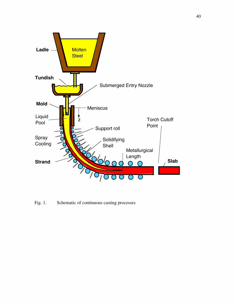
continuous casting process and the phenomena which govern it, illustrated in Figs. 1 and

2, make it difficult to model. However, with the increasing power of computer hardware

and software, mathematical modeling is becoming an important tool to understand all

aspects of the process.

1. Physical Models

Previous understanding of fluid flow in continuous casting has come about mainly

through experiments using physical water models. This technique is a useful way to test

and understand the effects of new configurations before implementing them in the

process. A full-scale model has the important additional benefit of providing operator

training and understanding.

Construction of a physical model is based on satisfying certain similitude criteria between

the model and actual process by matching both the geometry and the force balances that

govern the important phenomena of interest.[1-4] Some of the forces important to flow

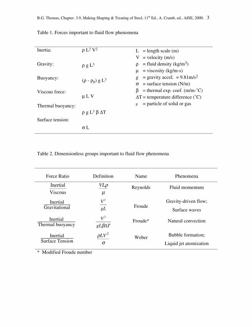
phenomena are listed in Table 1. To reproduce the molten steel flow pattern with a water

model, all of the ratios between the dominant forces must be the same in both systems.

Making, Shaping, and Treating of Steel, 11th Ed., A. Cramb, ed., AISE Steel Found., 2000.

This ensures that velocity ratios between the model and the steel process are the same at

every location. Table 2 shows some of the important force ratios in continuous casting

flows, which define dimensionless groups. The size of a dimensionless group indicates

the relative importance of two forces. Very small or very large groups can be ignored,

but all dimensionless groups of intermediate size in the steel process must be matched in

the physical model.

An appropriate geometry scale and fluid must be chosen to achieve these matches. It is

fortunate that water and steel have very similar kinematic viscosities (µ/ρ). Thus,

Reynolds and Froude numbers can be matched simultaneously by constructing a full

scale water model. Satisfying these two criteria is sufficient to achieve reasonable

accuracy in modeling isothermal single-phase flow systems, such as the continuous

casting nozzle and mold, which has been done with great success. A full-scale model has

the extra benefit of easy testing of plant components and operator training. Actually, a

water model of any geometric scale produces reasonable results for most of these flow

systems, so long as the velocities in both systems are high enough to produce fully

turbulent flow and very high Reynolds numbers. Because flow through the tundish and

mold nozzles are gravity driven, the Froude number is usually satisfied in any water

model of these systems where the hydraulic heads and geometries are all scaled by the

same amount.

Physical models sometimes must satisfy heat similitude criteria. In physical flow models

of steady flow in ladles and tundishes, for example, thermal buoyancy is large relative to

the dominant inertial-driven flow, as indicated by the size of the modified Froude

number, which therefore must be kept the same in the model as in the steel system. In

ladles, where velocities are difficult to estimate, it is convenient to examine the square of

the Reynolds number divided by the modified Froude number, which is called the

Grashof number. Inertia is dominant in the mold, so thermal buoyancy can be ignored

there. The relative magnitude of the thermal buoyancy forces can be matched in a full-

scale hot water model, for example, by controlling temperatures and heat losses such that

β∆T is the same in both model and caster. This is not easy, however, as the phenomena

B.G. Thomas, Chapter. 3.9, Making Shaping & Treating of Steel, 11th Ed., A. Cramb, ed., AISE, 2000. 3

Table 1. Forces important to fluid flow phenomena

Inertia:

Gravity:

Buoyancy:

Viscous force:

Thermal buoyancy:

Surface tension:

ρ L2 V2

ρ g L3

(ρ - ρp) g L3

µ L V

ρ g L3 β ∆T

σ L

L = length scale (m)V = velocity (m/s)ρ = fluid density (kg/m3)µ = viscosity (kg/m-s)g = gravity accel. = 9.81m/s2

σ = surface tension (N/m)β = thermal exp. coef. (m/m-˚C)∆T = temperature difference (˚C)p = particle of solid or gas

Table 2. Dimensionless groups important to fluid flow phenomena

Force Ratio Definition Name Phenomena

Inertial

Viscous

VLρµ

Reynolds Fluid momentum

InertialGravitational

V

gL

2

FroudeGravity-driven flow;

Surface waves

InertialThermal buoyancy

V

gL T

2

β∆Froude* Natural convection

InertialSurface Tension

ρσ

LV 2Weber Bubble formation;

Liquid jet atomization

* Modified Froude number


which govern heat losses depend on properties such as the fluid conductivity and specific

heat and the vessel wall conductivity, which are different in the model and the steel

vessel. In other systems, such as those involving low velocities, transients, or

solidification, simultaneously satisfying the many other similitude criteria important for

heat transfer is virtually impossible.

When physical flow models are used to study other phenomena, other force ratios must

be satisfied in addition to those already mentioned. For the study of inclusion particle

movement, for example, it is important to match the force ratios involving inertia, drag,

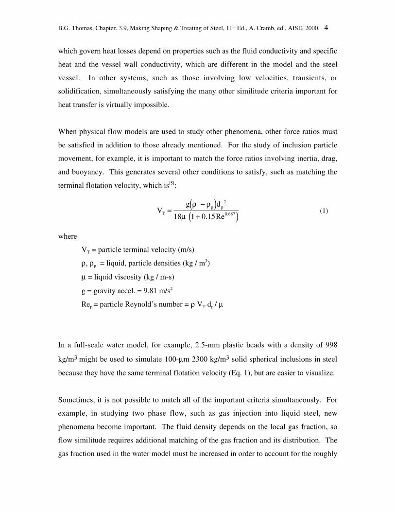
and buoyancy. This generates several other conditions to satisfy, such as matching the

terminal flotation velocity, which is[5]:

Vg d

T

p p=−( )

+( )ρ ρ

µ

2

0 68718 1 0 15. Re . (1)

where

VT = particle terminal velocity (m/s)

ρ, ρp = liquid, particle densities (kg / m3)

µ = liquid viscosity (kg / m-s)

g = gravity accel. = 9.81 m/s2

Rep = particle Reynold’s number = ρ VT dp / µ

In a full-scale water model, for example, 2.5-mm plastic beads with a density of 998

kg/m3 might be used to simulate 100-µm 2300 kg/m3 solid spherical inclusions in steel

because they have the same terminal flotation velocity (Eq. 1), but are easier to visualize.

Sometimes, it is not possible to match all of the important criteria simultaneously. For

example, in studying two phase flow, such as gas injection into liquid steel, new

phenomena become important. The fluid density depends on the local gas fraction, so

flow similitude requires additional matching of the gas fraction and its distribution. The

gas fraction used in the water model must be increased in order to account for the roughly


five-fold gas expansion that occurs when cold gas is injected into hot steel. Adjustments

must also be made for the local pressure, which also affects this expansion. In addition to

matching the gas fraction, the bubble size should be the same, so force ratios involving

surface tension, such as the Weber number, should also be matched. In attempting to

achieve this, it may be necessary to deviate from geometric similitude at the injection

point and to wax the model surfaces to modify the contact angles, in order to control the

initial bubble size. If gas momentum is important, such as for high gas injection rates,

then the ratio of the gas and liquid densities must also be the same. For this, helium in

water is a reasonable match for argon in steel. In many cases, it is extremely difficult to

simultaneously match all of the important force ratios. To the extent that this can be

approximately achieved, water modeling can reveal accurate insights into the real

process.

To quantify and visualize the flow, several different methods may be used. The easiest is

to inject innocuous amounts of gas, tracer beads, or die into the flow for direct

observation or photography. Quantitative mixing studies can measure concentration

profiles of other tracers, such as die with colorimetry measurement, salt solution with

electrical conductivity, or acid with pH tracking.[4] For all of these, it is important to

consider the relative densities of the tracer and the fluid. Accurate velocity

measurements, including turbulence measurements, may be obtained with hot wire

anemometry,[6] high speed videography with image analysis, particle image velocimetry

(PIV)[7, 8] or laser doppler velocimetry (LDV).[9] Depending on the phenomena of interest,

other parameters may be measured, such as pressure and level fluctuations on the top

surface.[10]

As an example, Fig. 3 shows the flow modeled in the mold region of a continuous thin-

slab caster.[11] The right side visualizes the flow using die tracer in a full-scale physical

water model. This particular caster features a 3-port nozzle that directs some of the flow

downward in order to stabilize the flow pattern from transient fluctuations and to

dissipate some of the momentum to lessen surface turbulence. The symmetrical left side


shows results from the other important analysis tool: computational modeling, which is

discussed in the next section.

2. Computational Models

In recent years, decreasing computational costs and increasing power of commercial

modeling packages is making it easier to apply mathematical models as an additional tool

to understand complex materials processes such as the continuous casting of steel.

Computational models have the advantage of easy extension to other phenomena such as

heat transfer, particle motion, and two-phase flow, which is difficult with isothermal

water models. They are also capable of more faithful representation of the flow

conditions experienced by the steel. For example, there is no need for the physical

bottom that interferes with the flow exiting a strand water model and the presence of the

moving solidifying shell can be taken into account.

Models can now simulate most of the phenomena important to continuous casting, which

include:

• fully-turbulent, transient fluid motion in a complex geometry (inlet nozzle and strand

liquid pool), affected by argon gas bubbles, thermal and solutal buoyancies

• thermodynamic reactions within and between the powder and steel phases

• flow and heat transport within the liquid and solid flux layers, which float on the top

surface of the steel

• dynamic motion of the free liquid surfaces and interfaces, including the effects of

surface tension, oscillation and gravity-induced waves, and flow in several phases

• transport of superheat through the turbulent molten steel

• transport of solute (including intermixing during a grade change)

• transport of complex-geometry inclusions through the liquid, including the effects of

buoyancy, turbulent interactions, and possible entrapment of the inclusions on nozzle

walls, gas bubbles, solidifying steel walls, and the top surface


• thermal, fluid, and mechanical interactions in the meniscus region between the

solidifying meniscus, solid slag rim, infiltrating molten flux, liquid steel, powder

layers, and inclusion particles.

• heat transport through the solidifying steel shell, the interface between shell and

mold, (which contains powder layers and growing air gaps) and the copper mold.

• mass transport of powder down the gap between shell and mold

• distortion and wear of the mold walls and support rolls

• nucleation of solid crystals, both in the melt and against mold walls

• solidification of the steel shell, including the growth of dendrites, grains and

microstructures, phase transformations, precipitate formation, and microsegregation

• shrinkage of the solidifying steel shell, due to thermal contraction, phase

transformations, and internal stresses

• stress generation within the solidifying steel shell, due to external forces, (mold

friction, bulging between the support rolls, withdrawal, gravity) thermal strains,

creep, and plasticity (which varies with temperature, grade, and cooling rate)

• crack formation

• coupled segregation, on both microscopic and macroscopic scales

The staggering complexity of this process makes it impossible to model all of these

phenomena together at once. Thus, it is necessary to make reasonable assumptions and to

uncouple or neglect the less-important phenomena. Quantitative modeling requires

incorporation of all of the phenomena that affect the specific issue of interest, so every

model needs a specific purpose. Once the governing equations have been chosen, they

are generally discretized and solved using finite-difference or finite-element methods. It

is important that adequate numerical validation be conducted. Numerical errors

commonly arise from too course a computational domain or incomplete convergence

when solving the nonlinear equations. Solving a known test problem and conducting

mesh refinement studies to achieve grid independent solutions are important ways to help

validate the model. Finally, a model must be checked against experimental

measurements on both the laboratory and plant scales before it can be trusted to make

quantitative predictions of the real process for a parametric study.


2.1 Heat Transfer and Solidification

Models to predict temperature and growth of the solidifying steel shell are used for basic

design, trouble shooting, and control of the continuous casting process.[12] These models

solve the transient heat conduction equation,

∂∂

ρ ∂∂

ρ ∂∂

∂∂t

Hx

v Hx

kT

xQ

ii

ieff

i

( ) + ( ) = ( ) + (2)

where ∂/∂t = differentiation with respect to time (s-1)

ρ = density (kg/m3)

H = enthalpy or heat content (J/kg)

xi = coordinate direction, x,y, or z (m)

vi = velocity component in xi direction (m/s)

keff = temperature-dependent effective thermal conductivity (W/m-K)

T = temperature field (K)

Q = heat sources (W/m3)

i = coordinate direction index which, when appearing twice in a term,

implies the summation of all three possible terms.

An appropriate boundary condition must be provided to define heat input to every portion

of the domain boundary, in addition to an initial condition (usually fixing temperature to

the pouring temperature). Latent heat evolution and heat capacity are incorporated into

the constitutive equation that must also be supplied to relate temperature with enthalpy.

Axial heat conduction can be ignored in models of steel continuous casting because it is

small relative to axial advection, as indicated by the small Peclet number (casting-speed

multiplied by shell thickness divided by thermal diffusivity). Thus, Lagrangian models

of a horizontal slice through the strand have been employed with great success for

steel.[13] These models drop the second term in Eq. 2 because velocity is zero in this

reference frame. The transient term is still included, even if the shell is withdrawn from


the bottom of the mold at a casting speed that matches the inflow of metal so the process

is assumed to operate at steady state.

Heat transfer in the mold region is controlled by :

• convection of liquid superheat to the shell surface

• solidification (latent heat evolution in the mushy zone)

• conduction through the solid shell

• the size and properties of the interface between the shell and the mold

• conduction through the copper mold

• convection to the mold cooling water

By far the most dominant of these is heat conduction across the interface between the

surface of the solidifying shell and the mold, although the solid shell also becomes

significant lower down. The greatest difficulty in accurate heat flow modeling is

determination of the heat transfer across this gap, qgap, which varies with time and

position depending on its thickness and the properties of the gas or lubricating flux layers

that fill it.

q hk

dT Tgap rad

gap

gapshell mold= +

−( )0 0 (3)

where qgap = local heat flux (W/m2)

hrad = radiation heat transfer coefficient across the gap (W/m2K)

kgap = effective thermal conductivity of the gap material (W/mK)

dgap = gap thickness (m)

T0shell = surface temperature of solidifying steel shell (K)

T0mold = hot face surface temperature of copper mold (K)

Usually, qgap is specified only as a function of distance down the mold, in order to match

a given set of mold thermocouple data.[14] However, where metal shrinkage is not

matched by taper of the mold walls, an air gap can form, especially in the corners. This


greatly reduces the heat flow locally. More complex models simulate the mold, interface,

and shell together, and use shrinkage models to predict the gap size.[15-17] This may allow

the predictions to be more generalized.

Mold heat flow models can feature a detailed treatment of the interface.[18-23] Some

include heat, mass, and momentum balances on the flux in the gap and the effect of shell

surface imperfections (oscillation marks) on heat flow and flux consumption.[23] This is

useful in steel slab casting operations with mold flux, for example, because hrad and kgap

both drop as the flux crystallizes and must be modeled properly in order to predict the

corresponding drop in heat transfer. The coupled effect of flow in the molten metal on

delivering superheat to the inside of the shell and thereby retarding solidification can also

be modeled quantitatively.[23, 24] Mold heat flow models can be used to identify deviations

from normal operation and thus predict quality problems such as impending breakouts or

surface depressions in time to take corrective action.

During the initial fraction of a second of solidification at the meniscus, a slight

undercooling of the liquid is required before nucleation of solid crystals can start. The

nuclei rapidly grow into dendrites, which evolve into grains and microstructures. These

phenomena can be modeled using microstructure models such as the cellular automata[25]

and phase field[26] methods. The latter requires coupling with the concentration field on a

very small scale so is very computationally intensive.

Below the mold, air mist and water spray cooling extract heat from the surface of the

strand. With the help of model calculations, cooling rates can be designed to avoid

detrimental surface temperature fluctuations. Online open-loop dynamic cooling models

can be employed to control the spray flow rates in order to ensure uniform surface

cooling even during transients, such as the temporary drop in casting speed required

during a nozzle or ladle change.[27]

The strand core eventually becomes fully solidified when it reaches the “metallurgical

length”. Heat flow models which extend below the mold are needed for basic machine


design to ensure that the last support roll and torch cutter are positioned beyond the

metallurgical length for the highest casting speed. A heat flow model can also be used to

trouble-shoot defects. For example, the location of a misaligned support roll that may be

generating internal hot-tear cracks can be identified by matching the position of the start

of the crack beneath the strand surface with the location of solidification front down the

caster calculated with a calibrated model.

2.2 Fluid Flow Models

Mathematical models of fluid flow can be applied to many different aspects of the

continuous casting process, including ladles, tundishes, nozzles, and molds.[12, 28] A

typical model solves the following continuity equation and Navier Stokes equations for

incompressible Newtonian fluids, which are based on conserving mass (one equation)

and momentum (three equations) at every point in a computational domain.[29, 30]

∂∂

v

xi

i

= 0 (4)

∂∂ ρ ∂

∂ ρ ∂∂

∂∂ µ ∂

∂∂∂ α ρ

tv

xv v P

x xvx

vx

T T g Fji

i ji i

effi

j

j

ij j+ = − + +

+ − +( )0

(5)

where ∂/∂t = differentiation with respect to time (s-1)


vi = velocity component in xi direction (m/s)


P = pressure field (N/m2)

µeff = effective viscosity (kg/m-s)

T = temperature field (K)

T0 = initial temperature (K)

α = thermal expansion coefficient, (m/m-K)

gj = magnitude of gravity in j direction (m/s2)

Fj = other body forces (eg. from eletromagnetic forces)


i, j = coordinate direction indices; which when repeated in a term, implies the

summation of all three possible terms.

The second last term in Eq. 5 accounts for the effect of thermal convection on the flow.

The last term accounts for other body forces, such as due to the application of

eletromagnetic fields. The solution of these equations yields the pressure and velocity

components at every point in the domain, which generally should be three dimensional.

At the high flow rates involved in these processes, these models must incorporate

turbulent fluid flow. The simplest, yet most computationally demanding, way to do this

is to use a fine enough grid (mesh) to capture all of the turbulent eddies and their motion

with time. This method, known as “direct numerical simulation”, was used to produce

the instantaneous velocity field in the mold cavity of a continuous steel slab caster shown

in Fig. 4.[7] The 30 seconds of flow simulated to achieve these results on a 1.5 million-

node mesh required 30 days of computation on an Origin 2000 supercomputer. The

calculations are compared with particle image velocimetry measurements of the flow in a

water model, shown on the right side of Fig. 4. These calculations reveal structures in the

flow pattern that are important to transient events such as the intermittent capture of

inclusion particles.

To achieve more computationally-efficient results, turbulence is usually modeled on a

courser grid using a time-averaged approximation, such as the K - ε model,[31] which

averages out the effect of turbulence using an increased effective viscosity field, µeff.

µ µ µ µ ρεµeff t C

K= + = +0 0

2

(6)

where µo , µt = laminar and turbulent viscosity fields (kg/m-s)

ρ = fluid density (kg/m3)

Cµ = empirical constant = 0.09

K = turbulent kinetic energy field, m2/s2

ε = turbulent dissipation field, m2/s3


This approach requires solving two additional partial differential equations for the

transport of turbulent kinetic energy and its dissipation:

ρ ∂∂

∂∂

µσ

∂∂

µ∂∂

∂∂

∂∂

ρεvK

x x

K

x

v

x

v

x

v

xjj j

t

K jt

j

i

i

j

j

i

=

+ +

− (7)

ρ ∂ε∂

∂∂

µσ

∂ε∂

µ ε ∂∂

∂∂

∂∂

ε ρεε

vx x x

CK

v

x

v

x

v

xC

Kjj j

t

jt

j

i

i

j

j

i

=

+ +

−1 2 (8)

where ∂/∂xi = differentiation with respect to coordinate direction x,y, or z (m)

K = turbulent kinetic energy field, m2/s2

ε = turbulent dissipation field, m2/s3


µt = turbulent viscosity (kg/m-s)

vi = velocity component in x, y, or z direction (m/s)

σK, σε = empirical constants (1.0, 1.3)

C1, C2 = empirical constants (1.44, 1.92)

i, j = coordinate direction indices; which when repeated in a term, implies the

summation of all three possible terms.

This approach generally uses special “wall functions” as the boundary conditions, in

order to achieve reasonable accuracy on a course grid.[31-33] Alternatively, a “low

Reynold’s number” turbulence model can be used, which models the boundary layer is a

more general way, but requires a finer mesh at the walls.[9, 34] An intermediate method

between direct numerical simulation and K-ε turbulence models, called “large eddy

simulation” uses a turbulence model only at the sub-grid scale.[35]

Most previous flow models have used the finite difference method, owing to the

availability of very fast and efficient solution methods.[36] Popular general-purpose codes

of this type include CFX,[37] FLUENT,[38] and PHOENICS.[39] Special-purpose codes of

this type include MAGMASOFT[40] and PHYSICA[41], which also solve for solidification


and temperature evolution in castings, coupled with mold filling. The finite element

method, such as used in FIDAP,[42] can also be applied and has the advantage of being

more easily adapted to arbitrary geometries, although it takes longer to execute. Special-

purpose codes of this type include PROCAST[43] and CAFE[44], which are popular for

investment casting processes.

Flow in the mold is of great interest because it influences many important phenomena,

which have far-reaching consequences on strand quality. Some of these phenomena are

illustrated in Fig. 2. They include the dissipation of superheat by the liquid jet impinging

upon the solidifying shell (and temperature at the meniscus), the flow and entrainment of

the top surface powder layers, top-surface contour and level fluctuations, and the

entrapment of subsurface inclusions and gas bubbles. Design compromises are needed to

simultaneously satisfy the contradictory requirements for avoiding each of these defect

mechanisms.

It is important to extend the simulation as far upstream as necessary to provide adequate

inlet boundary conditions for the domain of interest. For example, flow calculations in

the mold should be preceded by calculations of flow through the submerged entry nozzle.

This provides the velocities entering the mold in addition to the turbulence parameters, K,

and ε. Nozzle geometry greatly affects the flow in the mold and is easy to change, so is

an important subject for modeling.

The flow pattern changes radically with increasing argon injection rate, which requires

the solution of additional equations for the gas phase, and knowledge of the bubble size.[6, 37, 45] The flow pattern and mixing can also be altered by the application of

electromagnetic forces, which can either brake or stir the liquid. This can be modeled by

solving the Maxwell, Ohm, and charge conservation equations for electromagnetic forces

simultaneously with the flow model equations.[46] The great complexity which these

phenomena add to the coupled model equations make these calculations uncertain and a

subject of ongoing research.


2.3. Superheat Dissipation

An important task of the flow pattern is to deliver molten steel to the meniscus region that

has enough superheat during the critical first stages of solidification. Superheat is the

sensible heat contained in the liquid metal above the liquidus temperature and is

dissipated mainly in the mold.

The transport and removal of superheat is modeled by solving Eq. 2 using the velocities

found from the flow model (Eqs. 4-8). The effective thermal conductivity of the liquid is

proportional to the effective viscosity, which can be found from the turbulence

parameters (K and ε). The solidification front, which forms the boundary to the liquid

domain, can be treated in different ways. Many researchers model flow and solidification

as a coupled problem on a fixed grid.[25, 47, 48] Although very flexible, this approach is

subject to convergence difficulties and requires a fine grid to resolve the thin porous

mushy zone next to the thin shell.

An alternative approach for columnar solidification of a thin shell, such as found in the

mold for the continuous casting of steel, is to treat the boundary as a rough wall fixed at

the liquidus temperature using thermal wall laws.[49] Fig. 5 compares calculations using

this approach with measured temperatures in the liquid pool.[50] Incorporating the effects

of argon on the flow pattern were very important in achieving the reasonable agreement

observed. This figure shows that the temperature drops almost to the liquidus by mold

exit, indicating that most of the superheat is dissipated in the mold. Most of this heat is

delivered to the narrow face where the jet impinges, which is important to shell

solidification.[51]

The coldest regions are found at the meniscus at the top corners near the narrow face and

near the SEN. This is a concern because it could lead to freezing of the meniscus, and

encourage solidification of a thick slag rim. This could lead to quality problems such as

deep oscillation marks, cracks and other surface defects. In the extreme, the steel surface

can solidify a solid bridge between the SEN and the shell against the mold wall, which


often causes a breakout. To avoid these problems, flow must reach the surface quickly.

These calculations should be used, for example, to help design nozzle port geometries

that do not direct the flow too deep.

5. Top Surface Powder / Flux Layer Behavior

The flow of steel in the upper mold may influence the top surface powder layers, which

are very important to steel quality. Mold powder is added periodically to the top surface

of the steel. It sinters and melts to form a protective liquid flux layer, which helps to trap

impurities and inclusions. This liquid is drawn into the gap between the shell and mold

during oscillation, where it acts as a lubricant and helps to make heat transfer more

uniform. These phenomena are difficult to measure or to accurately simulate with a

physical model, so are worthy of mathematical modeling.

Fig. 6 shows results from a 3-D finite-element model of heat transfer and fluid flow in the

powder and flux layers, based on solving Eqs. 2, 4 and 5.[52] The bottom of the model

domain is the steel / flux interface. Its shape is imposed based on measurements in an

operating caster. Alternatively, this interface shape can be calculated by solving

additional equations to satisfy the force balance at the interface, which involves the

pressure in the two phases, shear forces from the moving fluids, surface tension, and

gravity.[53] For the conditions in this figure, the momentum of the flow up the narrow

face has raised the level of the interface there. The shear stress along the interface is

determined through coupled calculations with the 3-D steady flow model. The model

features different temperature-dependent flux properties for the interior, where the flux

viscosity during sintering before melting, compared with the region near the narrow face

mold walls, where the flux resolidifies to form a solid rim.

When molten steel flows rapidly along the steel / flux interface, it induces motion in the

flux layer. If the interface velocity becomes too high, then the liquid flux can be sheared

away from the interface, become entrained in the steel jet, and be sent deep into the liquid

pool to become trapped in the solidifying shell as a harmful inclusion. If the interface


velocity increases further, then the interface standing wave becomes unstable, and huge

level fluctuations contribute to further problems.

The thickness of the beneficial liquid flux layer is also very important. As shown in the

model calculations in Fig. 6, the liquid flux layer may become dangerously thin near the

narrow face if the steel flow tends to drag the liquid towards the center. This shortage of

flux feeding into the gap can lead to air gaps, reduced, non-uniform heat flow, thinning of

the shell, and longitudinal surface cracks. Quantifying these phenomena requires

modeling of both the steel flow and flux layers.

6. Motion and Entrapment of Inclusions and Gas Bubbles

The jets of molten steel exiting the nozzle may carry argon bubbles and inclusions such

as alumina into the mold cavity. These particles may create defects if they become

entrapped in the solidifying shell. Particle trajectories can be calculated using the

Langrangian particle tracking method, which solves a transport equation for each particle

as it travels through a previously-calculated velocity field.[34, 54, 55]

The force balance on each particle includes buoyancy and drag force relative to the

molten steel. The effects of turbulent motion can be modeled crudely from a K-ε flow

field by adding a random velocity fluctuation at each step, whose magnitude varies with

the local turbulent kinetic energy level. To obtain significant statistics, the trajectories of

several hundred individual particles should be calculated, using different starting points.

The bubbles collect inclusions, and inclusion clusters collide, so their size and shape

distributions evolve with time, which affects their drag and flotation velocities and

importance. Models are being developed to include these effects.[55]

Fig. 7 shows the trajectories of several particles moving through a steady flow field,

calculated using the K-ε model.[55] This simulation features particle trajectory tracking

that incorporates the influence of turbulence by giving a random velocity component to


the velocity at each time step in the calculation, in proportion to the local turbulence

level.

Most of the argon bubbles circulate in the upper mold area and float out to the top

surface. A few might be trapped at the meniscus if there is a solidification hook, and lead

to surface defects. A few small bubbles manage to penetrate into the lower recirculation

zone, where they move similarly to large inclusion clusters. Particles in this lower region

tend to move slowly in large spirals, while they float towards the inner radius of the slab.

When they eventually touch the solidifying shell in this deep region, entrapment is more

likely on the inside radius. Trapped argon bubbles elongate during rolling and in low-

strength steel, may expand during subsequent annealing processes to create costly surface

blisters and “pencil pipe" defects. Transient models are likely to yield further insights

into the complex and important phenomena of inclusion entrapment.

7. Composition Variation During Grade Changes

Large composition differences can arise through the thickness and along the length of the

final product due to intermixing after a change in steel grade during continuous casting.

Steel producers need to optimize casting conditions and grade sequences to minimize the

amount of steel downgraded or scrapped due to this intermixing. In addition, the

unintentional sale of intermixed product must be avoided. To do this requires knowledge

of the location and extent of the intermixed region and how it is affected by grade

specifications and casting conditions.

Models to predict intermixing must first simulate composition change in both the tundish

and in the liquid core of the strand as a function of time. This can be done using simple

lumped mixing-box models and / or by solving the mass diffusion equation in the flowing

liquid:

∂∂

∂∂

∂∂

∂∂

Ct

v Cx x

D Cxi

i ieff

i

+ = ( )(9)


In this equation, the composition, C, ranges between the old grade concentration of 0 and

the new grade concentration of 1. This dimensionless concept is useful because alloying

elements intermix essentially equally, owing to the much greater importance of turbulent

convection over laminar diffusion. In order to predict the final composition distribution

within the final product, a further model must account for the cessation of intermixing

after the shell has solidified.

Fig. 8 shows example composition distributions in a continuous cast slab calculated using

such a model.[56, 57] To ensure accuracy, extensive verification and calibration must be

undertaken for each submodel.[57] The tundish mixing submodel must be calibrated to

match chemical analysis of steel samples taken from the mold in the nozzle port exit

streams, or with tracer studies using full-scale water models. Accuracy of a simplified

strand submodel is demonstrated in Fig. 8 through comparison both with composition

measurements in a solidified slab and with a full 3-D model (Eq. 4).

The results in Fig. 8 clearly show the important difference between centerline and surface

composition. New grade penetrates deeply into the liquid cavity and contaminates the

old grade along the centerline. Old grade lingers in the tundish and mold cavity to

contaminate the surface composition of the new grade. This difference is particularly

evident in small tundish, thick-mold operations, where mixing in the strand is dominant.

Intermix models such as this one are in use at many steel companies. The model can be

enhanced to serve as an on-line tool by outputting for each grade change, the critical

distances which define the length of intermixed steel product which falls outside the

given composition specifications for the old and new grades.[57] In addition, it can be

applied off-line to perform parametric studies to evaluate the relative effects on the

amount of intermixed steel for different intermixing operations and for different

operating conditions using a standard ladle-exchange operation.[58] Finally, it can be used

to optimize scheduling and casting operation to minimize cost.


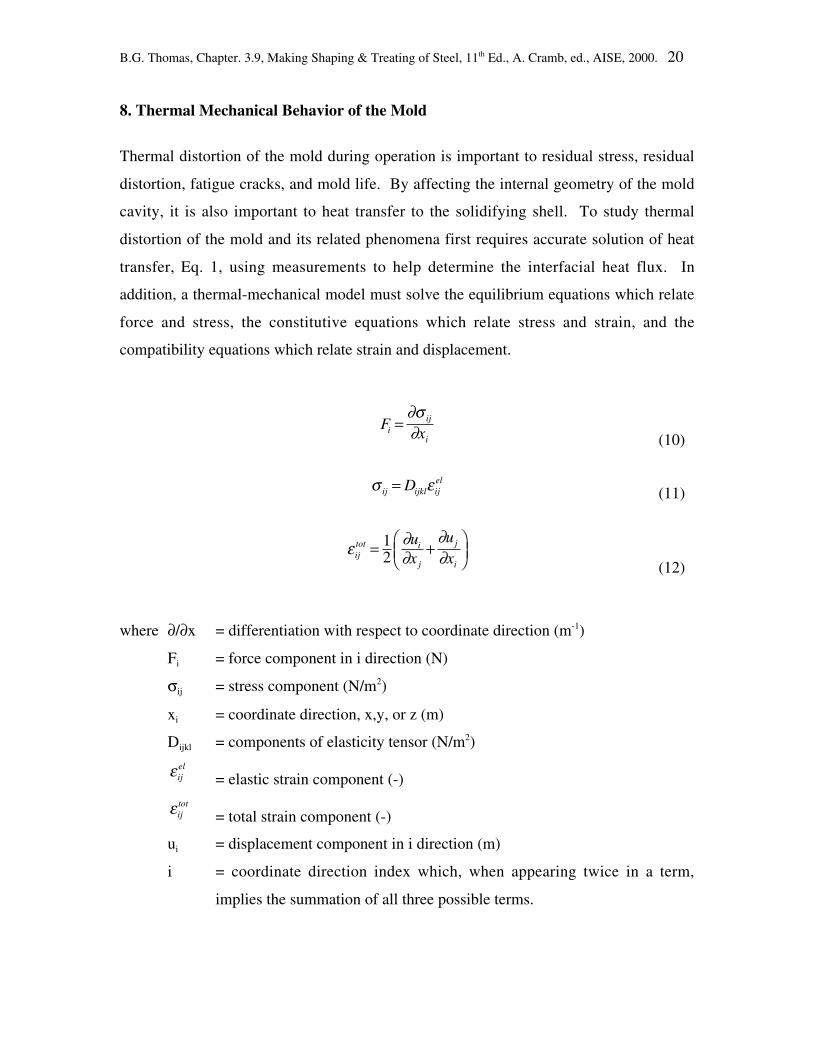
8. Thermal Mechanical Behavior of the Mold

Thermal distortion of the mold during operation is important to residual stress, residual

distortion, fatigue cracks, and mold life. By affecting the internal geometry of the mold

cavity, it is also important to heat transfer to the solidifying shell. To study thermal

distortion of the mold and its related phenomena first requires accurate solution of heat

transfer, Eq. 1, using measurements to help determine the interfacial heat flux. In

addition, a thermal-mechanical model must solve the equilibrium equations which relate

force and stress, the constitutive equations which relate stress and strain, and the

compatibility equations which relate strain and displacement.

Fxi

ij

i

=∂σ∂ (10)

σ εij ijkl ijelD= (11)

ε ∂∂

∂∂ij

tot i

j

j

i

ux

ux

= +

12

(12)

where ∂/∂x = differentiation with respect to coordinate direction (m-1)

Fi = force component in i direction (N)

σij = stress component (N/m2)


Dijkl = components of elasticity tensor (N/m2)

ε ijel

= elastic strain component (-)

ε ijtot

= total strain component (-)

ui = displacement component in i direction (m)

i = coordinate direction index which, when appearing twice in a term,

implies the summation of all three possible terms.


Thermal strain is found from the temperatures calculated in the heat transfer model and

accounts for the difference between the elastic and total strain. Further details are found

elsewhere.

In order to match the measured distortion, models should incorporate all of the important

geometric features of the mold, which often includes the four copper plates with their

water slots, reinforced steel water box assemblies, and tightened bolts. Three-

dimensional elastic-plastic-creep finite element models have been developed for slabs[59]

and thin slabs[60, 61] using the commercial finite-element package ABAQUS,[62] which is

well-suited to this nonlinear thermal stress problem. Their four-piece construction makes

slab molds behave very differently from a single-piece bloom or billet molds, which have

also been studied using thermal stress models.[63]

Fig. 9 illustrates typical temperature contours and the displaced shape calculated in one

quarter of the mold under steady operating conditions.[61] The hot exterior of each copper

plate attempts to expand, but is constrained by its colder interior and the cold, stiff, steel

water jacket. This makes each plate bend in towards the solidifying steel. Maximum

inward distortions of more than one millimeter are predicted just above the center of the

mold faces, and below the location of highest temperature, which is found just below the

meniscus.

The narrow face is free to rotate away from the wide face and contact only along a thin

vertical line at the front corner of the hot face. This hot edge must transmit all of the

clamping forces, so is prone to accelerated wear and crushing, especially during

automatic width changes. If steel enters the gaps formed by this mechanism, this can

lead to finning defects or even a sticker breakout. In addition, the widefaces may be

gouged, leading to longitudinal cracks and other surface defects.

The high compressive stress due to constrained thermal expansion induces creep in the

hot exterior of the copper plates which face the steel. This relaxes the stresses during


operation, but allows residual tensile stress to develop during cooling. Over time, these

cyclic thermal stresses and creep build up significant distortion of the mold plates. This

can contribute greatly to remachining requirements and reduced mold life. Under

adverse conditions, this stress could lead to cracking of the copper plates. The distortion

predictions are important for designing mold taper to avoid detrimental air gap formation.

These practical concerns can be investigated with quantitative modeling studies of the

effects of different process and mold design variables on mold temperature, distortion,

creep and residual stress. This type of stress model application will become more

important in the future to optimize the design of the new molds being developed for

continuous thin-slab and strip casting. For example, thermal distortion of the rolls during

operation of a twin-roll strip caster is on the same order as the section thickness of the

steel product.

9. Thermal Mechanical Behavior of the Shell

The solidifying shell is prone to a variety of distortion, cracking, and segregation

problems, owing to its creep at elevated temperature, combined with metallurgical

embrittlement and thermal stress. To start to investigate these problems, models are

being developed to simulate coupled fluid flow, thermal and mechanical behavior of the

solidifying steel shell during continuous casting.[17, 60, 64] The thermal-mechanical solution

procedure is documented elsewhere.[65] In addition to solving Eqs. 2, 3, 10, 11, and 12,

further constitutive equations are needed to characterize the inelastic creep and plastic

strains as a function of stress, temperature, and structure in order to accurately

incorporate the mechanical properties of the material. For example,[66]

ε̇ σ εεε

pn nQ

T= C exp [ a ] p

−

− (12)

where: ε̇p = inelastic strain rate (s-1)

σ = stress (MPa)

εp = inelastic strain (structure parameter)


T = temperature (K)

C,Q,aε,nc,n = empirical constants

Constitutive equations such as these are a subject of ongoing research because the

equations are difficult to develop, especially for complex loading conditions involving

stress reversals, the numerical methods to evaluate them are prone to instability, and the

experimental measurements they are based upon are difficult to conduct.

Thermal-mechanical models can be applied to predict the evolution of temperature,

stress, and deformation of the solidifying shell while in the mold for both billets[15] and

slabs.[16, 67-70] In this region, these phenomena are intimately coupled because the

shrinkage of the shell affects heat transfer across the air gap, which complicates the

calculation procedure. An example of the predicted temperature contours and distorted

shape of a transverse region near the corner is compared in Fig. 10 with measurements of

a breakout shell from an operating steel caster.[16] This model tracks the behavior of a

two-dimensional slice through the strand as it moves downward at the casting speed

through the mold and upper spray zones. It consists of separate finite-element models of

heat flow and stress generation that are step-wise coupled through the size of the

interfacial gap. The heat transfer model was calibrated using thermocouple

measurements down the centerline of the wideface for typical conditions. Shrinkage

predictions from the stress model are used to find the air gap thickness needed in Eq. 3 in

order to extend the calculations around the mold perimeter. The model includes the

effect of mold distortion on the air gaps, and superheat delivery from the flowing jet of

steel, calculated in separate models. The stress model includes ferrostatic pressure from

the molten steel on the inside of the shell and calculates intermittent contact between the

shell and the mold. It also features a temperature-dependent elastic modulus and an

elastic-viscoplastic constitutive equation that includes the effects of temperature,

composition, phase transformations and stress state on the local inelastic creep rate.

Efficient numerical algorithms are needed to integrate the equations.


As expected, good agreement is obtained in the region of good contact along the

wideface, where calibration was done. Near the corner along the narrow face, steel

shrinkage is seen to exceed the mold taper, which was insufficient. Thus, an air gap is

predicted. This air gap lowers heat extraction from the shell in the off-corner region of

the narrow face. When combined with high superheat delivery from the bifurcated

nozzle directed at this location, shell growth is greatly reduced locally. Just below the

mold, this thin region along the off-corner narrow-face shell caused the breakout.

Near the center of the narrow face, creep of the shell under ferrostatic pressure from the

liquid is seen to maintain contact with the mold, so much less thinning is observed. This

illustrates the tremendous effect that superheat has on slowing shell growth, if there is a

problem which lowers heat flow.

Fig. 11 presents sample distributions of temperature and stress through the thickness of

the shell, calculated with this model.[70] To achieve reasonable accuracy, a very fine mesh

and small time steps are needed. The temperature profile is almost linear through the

shell. The stress profile shows that the shell surface is in compression. This is because,

in the absence of friction with the mold, the surface layer solidifies and cools stress free.

As each inner layer solidifies, it cools and tries to shrink, while the surface temperature

remains relatively constant. The slab is constrained to remain planar, so complementary

subsurface tension and surface compression stresses are produced. To maintain force

equilibrium, note that the average stress through the shell thickness is zero. It is

significant that the maximum tensile stress is found near the solidification front. This

generic subsurface tensile stress is responsible for hot tear cracks, when accompanied by

metallurgical embrittlement.

Thermal-mechanical models such as this one can be applied to predict ideal mold

taper[71], to prevent breakouts such as the one discussed here[24] and to understand the

cause of other problems such as surface depressions[72] and longitudinal cracks. When

combined with transient temperature, flow and pressure calculations in the slag layers,


such models can simulate phenomena at the meniscus such as oscillation mark

formation.[73]

Computational models also can be applied to calculate thermomechanical behavior of the

solidifying shell below the mold. Models can investigate shell bulging between the

support rolls due to ferrostatic-pressure induced creep,[74-78] and the stresses induced

during unbending.[79] These models are important for the design of spray systems and

rolls in order to avoid internal hot tear cracks and centerline segregation. These models

face great numerical challenges because the phenomena are generally three dimensional

and transient, the constitutive equations are highly nonlinear, and the mechanical

behavior in one region (eg. the mold) may be coupled with the behavior very far away

(eg. unbending rolls).

10. Crack Formation

Although obviously of great interest, crack formation is particularly difficult to model

directly and is rarely attempted. Very small strains (on the order of 1%) can start hot tear

cracks at the grain boundaries if liquid metal is unable to feed through the secondary

dendrite arms to accommodate the shrinkage. Strain localization may occur on both the

small scale (when residual elements segregate to the grain boundaries) and on a larger

scale (within surface depressions or hot spots). Later sources of tensile stress, including

constraint due to friction and sticking, unsteady cooling below the mold, withdrawal

forces, bulging between support rolls, and unbending all worsen strain concentration and

promote crack growth. Microstructure, grain size and segregation are extremely

complex, so modeling of these phenomena is generally done independently of the stress

model. Of even greater difficulty for computational modeling is the great difference in

scale between these microstructural phenomena relative to the size of the casting, where

the important macroscopic temperature and stress fields develop.

Considering this complexity, the results of macroscopic thermal-stress models are linked

to the microstructural phenomena that control crack initiation and propagation through


the use of fracture criteria. To predict hot-tear cracks, most fracture criteria identify a

critical amount of inelastic strain (eg. 1 – 3.8%) accumulated over a critical range of

liquid fraction, fL, such as 0.01< fL <0.2 [80, 81]. Recent work suggests that the fracture

criterion should consider the inelastic strain rate, which is important during liquid feeding

through a permeable region of dendrite arms in the mushy zone.[82] Careful experiments

are needed to develop these fracture criteria by applying stress during solidification.[83] [84,

85] There experiments are difficult to control so detailed modeling of the experiment itself

is becoming necessary, in order to extract more fundamental material properties such as

fracture criteria.

11. Centerline Segregation

Macrosegregation near the centerline of the solidified slab is detrimental to product

properties, particularly for highly alloyed steels, which experience the most segregation.

Centerline segregation can be reduced and even avoided through careful application of

eletromagnetic forces, and soft reduction, where the slab is rolled or quenched just before

it is fully solidified. Computational modeling would be useful to help understand and

optimize these practices.

Centerline segregation is a very difficult problem to simulate, because such a wide range

of coupled phenomena must be properly modelled. Bulging between the rolls and

solidification shrinkage together drive the fluid flow necessary for macrosegregation, so

fluid flow, solidification heat transfer, and stresses must all be modeled accurately

(including Eqs. 2, 4, 5, 10, 12, and 13). The microstructure is also important, as equiaxed

crystals behave differently than columnar grains, so must also be modeled. This is

complicated by the convection of crystals in the molten pool in the strand, which depends

on both flow from the nozzle and thermal / solutal convection. Increasing superheat

tends to worsen segregation, so the details of mold superheat transfer must also be

properly modeled. Naturally, Eq. 8 must be solved for each important alloying element

on both the microstructural scale (between dendrite arms), with the help of

microsegregation software such as THERMOCALC,[86] and on the macroscopic scale


(from surface to center of the strand), using advanced computations.[48, 87] The diffusion

coefficients and partition coefficients needed for this calculation are not currently known

with sufficient accuracy. Finally, the application of eletromagnetic and roll forces

generate additional modeling complexity. Although the task appears overwhelming,

steps are being taken to model this important problem.[88, 89]

Much further work is needed to understand and quantify these phenomena and to apply

the results to optimize the continuous casting process. In striving towards these goals, the

importance of combining modeling and experiments together cannot be overemphasized.

Conclusion

The final test of a model is if the results can be implemented into practice and

improvements can be achieved, such as the avoidance of defects in the steel product.

Plant trials are ultimately needed for this implementation. Trials should be conducted on

the basis of insights supplied from all available sources, including physical models,

mathematical models, literature, and previous experience.

As increasing computational power continues to advance the capabilities of numerical

simulation tools, modeling should play an increasing role in future advances to high-

technology processes such as the continuous casting of steel. Modeling can augment

traditional research methods in generating and quantifying the understanding needed to

improve any aspect of the process. Areas where advanced computational modeling

should play a crucial role in future improvements include transient flow simulation, mold

flux behavior, taper design, online quality prediction and control, especially for new

problems and processes such as high speed billet casting, thin slab casting, and strip

casting.

Future advances to the continuous casting process will not come from either models,

experiments, or plant trials. They will come from ideas generated by people who


understand the process and the problems. This understanding is rooted in knowledge,

which can be confirmed, deepened, and quantified by tools which include computational

models. As our computational tools continue to improve, they should grow in

importance in fulfilling this important role, leading to future process advances.


List of Figures

Fig. 1. Schematic of continuous casting processes

Fig. 2. Schematic of phenomena in the mold region of a steel slab caster

Fig. 3. Flow in a thin slab casting mold visualized using a) K-ε computer simulation

b) water model with die injection [11]

Fig. 4. Instantaneous flow pattern in a slab casting mold comparing LES simulation (left)

and PIV measurement (right) [7]

Fig. 5. Temperature distribution in mold showing superheat dissipation [50]

Fig. 6. Comparison of measured and predicted melt-interface positions [52]

Fig. 7. Sample trajectories of 0.3 mm argon bubbles with turbulent motion [55]

Fig. 8. Predicted composition distribution in a steel slab cast during a grade change

compared with experiments [57]

Fig. 9. Distorted shape of thin slab casting mold during operation (50 X

magnification) with temperature contours (˚C) [61]

Fig. 10. Comparison between predicted and measured shell thickness in a horizontal

(x-y) section through the corner of a continuous-cast steel breakout shell [16]

Fig. 11. Typical Temperature and Stress distributions through shell thickness [70]


References

1. J. Szekely, J.W. Evans and J.K. Brimacombe, The Mathematical and Physical

Modeling of Primary Metals Processing Operations, (New York, NY: John Wiley

& Sons, 1987).

2. J. Szekely and N. Themelis, Rate Phenomena in Process Metallurgy, (New York,

NY: Wiley-Interscience, 1971), 515-597.

3. R.I.L. Guthrie, Engineering in Process Metallurgy, (Oxford, UK: Clarendon Press,

1992), 528.

4. L.J. Heaslip and J. Schade, "Physical Modeling and Visualization of Liquid Steel

Flow Behavior During Continuous Casting," Iron & Steelmaker, 26 (1) (1999), 33-

41.

5. S.L. Lee, "Particle Drag in a Dilute Turbulent Two-Phase Suspension Flow,"

Journal of Multiphase Flow, 13 (2) (1987), 247.

6. B.G. Thomas, X. Huang and R.C. Sussman, "Simulation of Argon Gas Flow

Effects in a Continuous Slab Caster," Metall. Trans. B, 25B (4) (1994), 527-547.

7. S. Sivaramakrishnan, H. Bai, B.G. Thomas, P. Vanka, P. Dauby, M. Assar,

"Transient Flow Structures in Continuous Cast Steel," in Ironmaking Conference

Proceedings, 59, (Pittsburgh, PA: ISS, Warrendale, PA, 2000), 541-557.

8. M.B. Assar, P.H. Dauby and G.D. Lawson, "Opening the Black Box: PIV and

MFC Measurements in a Continuous Caster Mold," in Steelmaking Conference

Proceedings, 83, (ISS, Warrendale, PA, 2000), 397-411.

9. X.K. Lan, J.M. Khodadadi and F. Shen, "Evaluation of Six k- Turbulence Model

Predictions of Flowin a Continuous Casting Billet-Mold Water Model Using Laser

Doppler Velocimetry Measurements," Metall. Mater. Trans., 28B (2) (1997), 321-

332.


10. J. Herbertson, Q.L. He, P.J. Flint, R.B. Mahapatra, "Modelling of Metal Delivery

to Continuous Casting Moulds," in Steelmaking Conf. Proceedings, 74, (ISS,

Warrendale, PA, 1991), 171-185.

11. B.G. Thomas, R. O'Malley, T. Shi, Y. Meng, D. Creech, D. Stone, "Validation of

Fluid Flow and Solidification Simulation of a Continuous Thin Slab Caster," in

Modeling of Casting, Welding, and Advanced Solidification Processes, IX,

(Aachen, Germany, August 20-25, 2000: Shaker Verlag GmbH, Aachen, Germany,

2000), 769-776.

12. B.G. Thomas, "Mathematical Modeling of the Continuous Slab Casting Mold : A

State of the Art Review," in 74th Steelmaking Conference Proceedings, 74, (ISS,

Warrendale, PA, 1991), 105-118.

13. J. Lait, J.K. Brimacombe and F. Weinberg, "Mathematical Modelling of Heat Flow

in the Continuous Casting of Steel," Ironmaking and Steelmaking, 2 (1974), 90-98.

14. R.B. Mahapatra, J.K. Brimacombe and I.V. Samarasekera, "Mold Behavior and its

Influence on Quality in the Continuous Casting of Slabs: Part I. Industiral Trials,

Mold Temperature Measurements, and Mathematical Modelling," Metallurgical

Transactions B, 22B (December) (1991), 861-874.

15. J.E. Kelly, K.P. Michalek, T.G. O'Connor, B.G. Thomas, J.A. Dantzig, "Initial

Development of Thermal and Stress Fields in Continuously Cast Steel Billets,"

Metallurgical Transactions A, 19A (10) (1988), 2589-2602.

16. A. Moitra and B.G. Thomas, "Application of a Thermo-Mechanical Finite Element

Model of Steel Shell Behavior in the Continuous Slab Casting Mold," in

Steelmaking Proceedings, 76, (Dallas, TX: Iron and Steel Society, 1993), 657-667.

17. J.-E. Lee, T.-J. Yeo, K.H. Oh, J.-K. Yoon, U.-S. Yoon, "Prediction of Cracks in

Continuously Cast Beam Blank through Fully Coupled Analysis of Fluid Flow,

Heat Transfer and Deformation behavior of Solidifying Shell," Metall. Mater.

Trans. A, 31A (1) (2000), 225 - 237.


18. R. Bommaraju and E. Saad, "Mathematical modelling of lubrication capacity of

mold fluxes," in Steelmaking Proceedings, 73, (Warrendale, PA: Iron and Steel

Society, 1990), 281-296.

19. B.G. Thomas and B. Ho, "Spread Sheet Model of Continuous Casting," J.

Engineering Industry, 118 (1) (1996), 37-44.

20. B. Ho, "Characterization of Interfacial Heat Transfer in the Continuous Slab

Casting Process" (Masters Thesis, University of Illinois at Urbana-Champaign,

1992).

21. J.A. DiLellio and G.W. Young, "An Asymptotic Model of the Mold Region in a

Continuous Steel Caster," Metall. Mater. Trans., 26B (6) (1995), 1225-1241.

22. B.G. Thomas, D. Lui and B. Ho, "Effect of Transverse and Oscillation Marks on

Heat Transfer in the Continuous Casting Mold," in Applications of Sensors in

Materials Processing, V. Viswanathan, ed. (Orlando, FL: TMS, Warrendale, PA,

1997), 117-142.

23. B.G. Thomas, B. Ho and G. Li, "Heat Flow Model of the Continuous Slab Casting

Mold, Interface, and Shell," in Alex McLean Symposium Proceedings, Toronto,

(Warrendale, PA: Iron and Steel Society, 1998), 177-193.

24. G.D. Lawson, S.C. Sander, W.H. Emling, A. Moitra, B.G. Thomas, "Prevention of

Shell Thinning Breakouts Associated with Widening Width Changes," in

Steelmaking Conference Proceedings, 77, (Warrendale, PA: Iron and Steel

Society, 1994), 329-336.

25. C.-A. Gandin, T. Jalanti and M. Rappaz, "Modeling of Dendritic Grain Structures,"

in Modeling of Casting, Welding, and Advanced Solidification Processes, VIII,

B.G. Thomas and C. Beckermann, eds., (TMS, Warrendale, PA, 1998), 363-374.

26. I. Steinbach and G.J. Schmitz, "Direct Numerical Simulation of Solidification

Structure using the Phase Field Method," in Modeling of Casting, Welding, and

Advanced Solidification Processes, VIII, B.G. Thomas and C. Beckermann, eds.,

(TMS, Warrendale, PA, 1998), 521-532.


27. R.A. Hardin, K. Liu and C. Beckermann, "Development of a Model for Transient

Simulation and Control of a Continuous Steel Slab Caster," in Materials

Processing in the Computer Age, 3, (Minerals, Metals, & Materials Society,

Warrendale, PA, 2000), 61-74.

28. J. Szekely and R.T. Yadoya, "The Physical and Mathematical Modelling of the

Flow Field in teh Mold Region of Continuous casitng Units. Part II. Computer

Solution of the Turbulent Flow Equations," Metall. Mater. Trans., 4 (1973), 1379.

29. S.V. Patankar, Numerical Heat Transfer and Fluid Flow, (New York, NY:

McGraw Hill, 1980).

30. S.V. Patankar and B.D. Spalding, "A calculation procedure for heat, mass and

momentum transer in three-dimensional parabolic flows," Int. J. Heat Mass

Transfer, 15 (1992), 1787-1806.

31. B.E. Launder and D.B. Spalding, "Numerical Computation of Turbulent Flows,"

Computer Methods in Applied Mechanics and Engr, 13 (1974), 269-289.

32. B.G. Thomas and F.M. Najjar, "Finite-Element Modeling of Turbulent Fluid Flow

and Heat Transfer in Continuous Casting," Applied Mathematical Modeling, 15

(1991), 226-243.

33. D.E. Hershey, B.G. Thomas and F.M. Najjar, "Turbulent Flow through Bifurcated

Nozzles," International Journal for Numerical Methods in Fluids, 17 (1993), 23-47.

34. M.R. Aboutalebi, M. Hasan and R.I.L. Guthrie, "Coupled Turbulent Flow, Heat,

and Solute Transport in Continuous Casting Processes," Metall. Mater. Trans., 26B

(4) (1995), 731-744.

35. J. Smagorinsky, "General Circulation Experiments With the Primitive Equations"

(Report, Weather Bureau: Washington, 1963), 99-121.

36. N.C. Markatos, "Computational fluid flow capabilities and software," Ironmaking

and Steelmaking, 16 (4) (1989), 266-273.


37. "CFX 4.2," (AEA Technology, 1700 N. Highland Rd., Suite 400, Pittsburgh, PA

15241, 1998 ).

38. "FLUENT 5.1," (Fluent Inc., Lebanon, New Hampshire, 2000 ).

39. "PHOENICS," (CHAM, Wimbledon Village, London, UK, 2000 ).

40. E. Flender, "MAGMASOFT," (Magma Gmbh, Aachen, Germany, 2000 ).

41. M. Cross, "PHYSICA," (Computing & Math Sciences, Maritime Greenwich

University, Greenwich, UK, 2000 ).

42. M.S. Engleman, "FIDAP 8.5," (Fluent, Inc., 500 Davis Ave., Suite 400, Evanston,

IL 60201, 2000 ).

43. M. Sammonds, "PROCAST," (UES Software, 175 Admiral Cochrane Dr.,

Annapolis, MD, 2000 ).

44. P. Thevoz, "CAFE," (CALCOM, EPFL, Lausanne, Switzerland, 2000 ).

45. N. Bessho, R. Yoda, H. Yamasaki, T. Fujii, T. Nozaki, "Numerical Analysis of

Fluid Flow in the Continuous Casting Mold by a Bubble Dispersion Model," Iron

and Steelmaker, 18 (4) (1991), 39-44.

46. T. Ishii, S.S. Sazhin and M. Makhlouf, "Numerical prediction of

magnetohydrodynamic flow in continuous casting process," Ironmaking and

Steelmaking, 23 (3) (1996), 267-272.

47. V.R. Voller, A.D. Brent and C. Prakash, "The Modelling of Heat, Mass and Solute

Transport in Solidification Systems," Applied Mathematical Modelling, 32 (1989),

1719-1731.

48. M.C. Schneider and C. Beckermann, "The Formation of Macrosegregation by

Multicomponent Thermosolutal Convection during the Solidification of Steel,"

Metall. Mater. Trans. A, 26A (1995), 2373-2388.


49. X. Huang, B.G. Thomas and F.M. Najjar, "Modeling Superheat Removal during

Continuous Casting of Steel Slabs," Metallurgical Transactions B, 23B (6) (1992),

339-356.

50. B.G. Thomas, "Continuous Casting of Steel, Chap. 15," in Modeling and

Simulation for Casting and Solidification: Theory and Applications, O. Yu, ed.

(Marcel Dekker, New York, 2000).

51. H. Nakato, M. Ozawa, K. Kinoshita, Y. Habu, T. Emi, "Factors Affecting the

Formation of Shell and Longitudinal Cracks in Mold during High Speed

Continuous Casting of Slabs," Trans. Iron Steel Inst. Japan, 24 (11) (1984), 957-

965.

52. R. McDavid and B.G. Thomas, "Flow and Thermal Behavior of the Top-Surface

Flux/ Powder Layers in Continuous Casting Molds," Metallurgical Transactions B,

27B (4) (1996), 672-685.

53. G.A. Panaras, A. Theodorakakos and G. Bergeles, "Numerical Investigation of the

Free Surface in a continuous Steel Casting Mold Model," Metall. Mater. Trans. B,

29B (5) (1998), 1117-1126.

54. R.C. Sussman, M. Burns, X. Huang, B.G. Thomas, "Inclusion Particle Behavior in

a Continuous Slab Casting Mold," in 10th Process Technology Conference Proc.,

10, (Toronto, Canada: Iron and Steel Society, Warrendale, PA, 1992), 291-304.

55. B.G. Thomas, A. Dennisov and H. Bai, "Behavior of Argon Bubbles during

Continuous Casting of Steel," in Steelmaking Conference Proceedings, 80,

(Chicago, IL: ISS, Warrendale, PA., 1997), 375-384.

56. X. Huang and B.G. Thomas, "Modeling of Steel Grade Transition in Continuous

Slab Casting Processes," Metallurgical Transactions, 24B (1993), 379-393.

57. X. Huang and B.G. Thomas, "Intermixing Model of Continuous Casting During a

Grade Transition," Metallurgical Transactions B, 27B (4) (1996), 617-632.

58. B.G. Thomas, "Modeling Study of Intermixing in Tundish and Strand during a

Continuous-Casting Grade Transition," ISS Transactions, 24 (12) (1997), 83-96.


59. B.G. Thomas, G. Li, A. Moitra, D. Habing, "Analysis of Thermal and Mechanical

Behavior of Copper Molds during Continuous Casting of Steel Slabs," Iron and

Steelmaker (ISS Transactions), 25 (10) (1998), 125-143.

60. T. O'Conner and J. Dantzig, "Modeling the Thin Slab Continuous Casting Mold,"

Metall. Mater. Trans., 25B (4) (1994), 443-457.

61. J.-K. Park, I.V. Samarasekera, B.G. Thomas, U.-S. Yoon, "Analysis of Thermal

and Mechanical Behavior of Copper Mould During Thin Slab Casting," in

Steelmaking Conference Proceedings, 83, (ISS, Warrendale, PA:, 2000), 9-21.

62. "ABAQUS 5.8," (Hibbitt, Karlsson & Sorensen, Inc., 1080 Main Street,

Pawtucket, Rhode Island 02860, 1999 ).

63. I.V. Samarasekera, D.L. Anderson and J.K. Brimacombe, "The Thermal Distortion

of Continuous Casting Billet Molds," Metallurgical Transactions B, 13B (March)

(1982), 91-104.

64. A. Cristallini, M.R. Ridolfi, A. Spaccarotella, R. Capotosti, G. Flemming, J.

Sucker, "Advanced Process Modeling of CSP Funnel Design for Thin Slab Casting

of High Alloyed Steels," in Seminario de Aceria of the Instituto Argentino de

Siderurgia (IAS) Proceedings, (IAS, Buones Aires, Argentina, 1999), 468-477.

65. J.A. Dantzig, "Thermal stress development in metal casting processes,"

Metallurgical Science and Technology, 7 (3) (1989), 133-178.

66. P. Kozlowski, B.G. Thomas, J. Azzi, H. Wang, "Simple Constitutive Equations for

Steel at High Temperature," Metallurgical Transactions A, 23A (March) (1992),

903-918.

67. K. Sorimachi and J.K. Brimacombe, "Improvements in mathematical modelling of

stresses in continuous casting of steel," Ironmaking and Steelmaking, (4) (1977),

240-245.

68. K. Kinoshita, H. Kitaoka and T. Emi, "Influence of Casting Conditions on the

Solidification of Steel Melt in Continuous Casting Mold," Tetsu-to-Hagane, 67 (1)

(1981), 93-102.


69. I. Ohnaka and Y. Yashima, "Stress Analysis of Steel Shell Solidifying in

Continuous Casting Mold," in Modeling of Casting and Welding Processes IV, 4,

(Minerals, Metals, and Materials Society, Warrendale, PA, 1988), 385-394.

70. B.G. Thomas and J.T. Parkman, "Simulation of Thermal Mechanical Behavior

during Initial Solidification," in Thermec 97 Internat. Conf. on Thermomechanical

Processing of Steel and Other Materials, 2, T. Chandra, ed. (Wollongong,

Australia: TMS, 1997), 2279-2285.

71. B.G. Thomas, A. Moitra and W.R. Storkman, "Optimizing Taper in Continuous

Slab Casting Molds Using Mathematical Models," in Proceedings, 6th

International Iron and Steel Congress, 3, (Nagoya, Japan: Iron & Steel Inst. Japan,

Tokyo, 1990), 348-355.

72. B.G. Thomas, A. Moitra and R. McDavid, "Simulation of Longitudinal Off-Corner

Depressions in Continuously-Cast Steel Slabs," ISS Transactions, 23 (4) (1996),

57-70.

73. K. Schwerdtfeger and H. Sha, "Depth of Oscillation Marks Forming in Continuous

Casting of Steel," Metallurgical and Materials Transactions A, in press (1999),

74. A. Palmaers, A. Etienne and J. Mignon, "Calculation of the Mechanical and

Thermal Stresses in Continuously Cast Strands, in german," Stahl und Eisen, 99

(19) (1979), 1039-1050.

75. J.B. Dalin and J.L. Chenot, "Finite element computation of bulging in continuously

cast steel with a viscoplastic model," International Journal for Numerical Methods

in Engineering, 25 (1988), 147-163.

76. B. Barber and A. Perkins, "Strand Deformation in continuous casting," Ironmaking

and Steelmaking, 16 (6) (1989), 406-411.

77. K. Okamura and H. Kawashima, "Calculation of Bulging Strain and its

Application to Prediction of Internal Cracks in Continuously Cast Slabs," in Proc.

Int. Conf. Comp. Ass. Mat. Design Proc. Simul., (ISIJ, Tokyo, 1993), 129-134.


78. L. Yu, "Bulging in Continuous Cast Steel Slabs" (M.S. Thesis, University of

Illinois, 2000).

79. M. Uehara, I.V. Samarasekera and J.K. Brimacombe, "Mathematical modelling fo

unbending of continuously cast steel slabs," Ironmaking and Steelmaking, 13 (3)

(1986), 138.

80. T.W. Clyne and G.J. Davies, "The influence of composition on solidification

cracking susceptibiltity in binary alloy systems," Br. Foundrymen, 74 (4) (1981),

65-73.

81. A. Yamanaka, K. Nakajima and K. Okamura, "Critical strain for internal crack

formation in continuous casting," Ironmaking and Steelmaking, 22 (6) (1995), 508-

512.

82. M. Rappaz, J.-M. Drezet and M. Gremaud, "A New Hot-Tearing Criterion,"

Metall. Mater. Trans. A, 30A (2) (1999), 449-455.

83. T. Matsumiya, M. Ito, H. Kajioka, S. Yamaguchi, Y. Nakamura, "An Evaluation of

Critical Strain for Internal Crack Formation in Continuously Cast Slabs,"

Transactions of the Iron and Steel Institute of Japan, 26 (1986), 540-546.

84. C. Bernhard, H. Hiebler and M.M. Wolf, "Experimental simulation of subsurface

crack formation in continuous casting," Rev. Metall., march (2000), 333-344.

85. C.H. Yu, M. Suzuki, H. Shibata, T. Emi, "Simulation of Crack Formation on

Solidifying Steel Sheel in Continuous Casting Mold," ISIJ International, 36

(1996), S159-S162.

86. B. Sundman, B. Jansson and J.O. Anderson, "The Thermo-Calc Databank

System," CALPHAD 9, 2 (1985), 153-190.

87. C.Y. Wang and C. Beckermann, "Equiaxed Dendritic Solidification with

Convection," Metall. Mater. Trans. A, 27A (9) (1996), 2754-2764.


88. T. Kajitani, J.-M. Drezet and M. Rappaz, "Numerical simulation of deformation-

induced segregation in continuous casting of steel," Metall. Mater. Trans., (2001),

in press.

89. G. Lesoult and S. Sella, Solid State Phenomena, 3 (1988), 167-178.

40

Ladle

Tundish

Submerged Entry Nozzle

Mold

SprayCooling

Torch Cutoff Point

Molten Steel

Slab

Metallurgical Length

Liquid Pool

Strand

Solidifying Shell

Meniscus

z

Support roll

Fig. 1. Schematic of continuous casting processes

41

Water

Spray

Molten Steel Pool

Solidifying Steel Shell

Flux Rim

Submerged Entry Nozzle

SupportRoll

Roll Contact

Ferrostatic Pressure

Bulging

Roll

Nozzle

Nozzle

coppermold

Liquid Flux

Air Gap

Flux Powder

jet

nozzle portargon

bubbles

Inclusion particles and bubbles

Resolidified Flux

Contact Resistances

Oscillation Mark

entrainment

CL

Fig. 2. Schematic of phenomena in the mold region of a steel slab caster

42

a) b)

Fig. 3. Flow in a thin slab casting mold visualized using a) K-ε computer simulationb) water model with die injection [11]

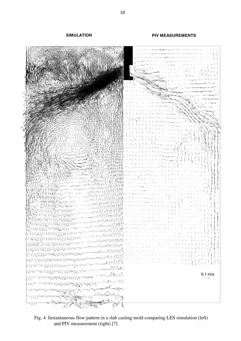
SIMULATION PIV MEASUREMENTS

0.1 m/s

Fig. 4 Instantaneous flow pattern in a slab casting mold comparing LES simulation (left) and PIV measurement (right) [7]

18

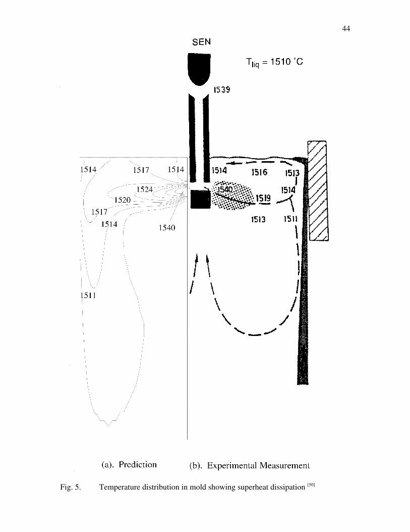
44

Fig. 5. Temperature distribution in mold showing superheat dissipation [50]

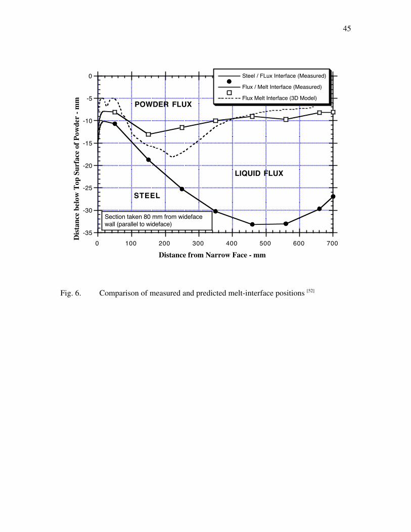
45

-35

-30

-25

-20

-15

-10

-5

0

0 100 200 300 400 500 600 700

Steel / FLux Interface (Measured)

Flux / Melt Interface (Measured)

Flux Melt Interface (3D Model)

Dis

tanc

e be

low

Top

Sur

face

of

Pow

der

- m

m

Distance from Narrow Face - mm

Section taken 80 mm from wideface wall (parallel to wideface)

STEEL

LIQUID FLUX

POWDER FLUX

Fig. 6. Comparison of measured and predicted melt-interface positions [52]

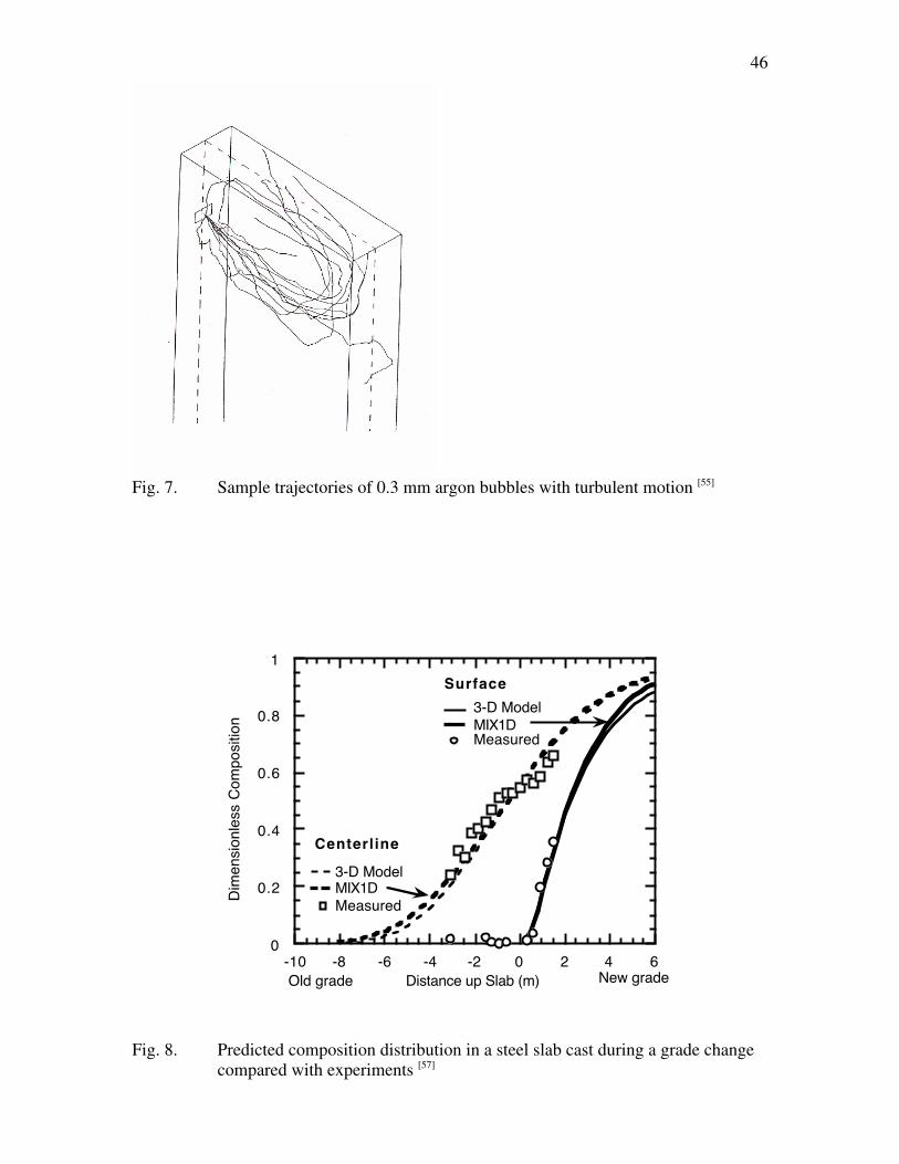
46

Fig. 7. Sample trajectories of 0.3 mm argon bubbles with turbulent motion [55]

0

0.2

0.4

0.6

0.8

1

-10 -8 -6 -4 -2 0 2 4 6

Dim

ensi

onle

ss C

ompo

sitio

n

Distance up Slab (m)

MIX1D3-D Model

Measured

Surface

3-D ModelMIX1DMeasured

Centerline

New gradeOld grade

Fig. 8. Predicted composition distribution in a steel slab cast during a grade changecompared with experiments [57]

47

138o

411o

356o

302o

247o

247o

Fig. 9. Distorted shape of thin slab casting mold during operation (50 Xmagnification) with temperature contours (˚C) [61]

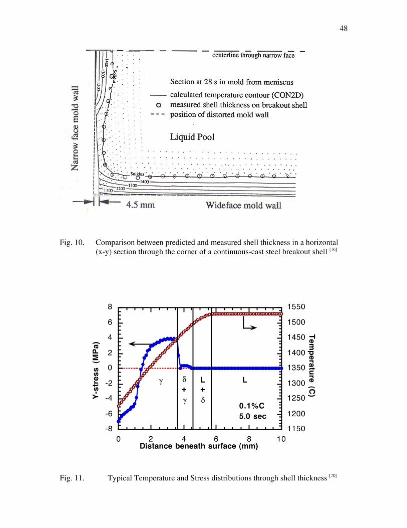
48

Fig. 10. Comparison between predicted and measured shell thickness in a horizontal(x-y) section through the corner of a continuous-cast steel breakout shell [16]

-8

-6

-4

-2

0

2

4

6

8

1150

1200

1250

1300

1350

1400

1450

1500

1550

0 2 4 6 8 10

Y-s

tres

s (M

Pa)

Tem

peratu

re (C)

Distance beneath surface (mm)

L+δ

δ+γ

γ L

0.1%C5.0 sec

Fig. 11. Typical Temperature and Stress distributions through shell thickness [70]

chapter 3.9 fundamentals of continuous casting:...

Documents