chapter 4 – data mining a short introductionlsir minin… · · 2007-02-053 ©2006/7, karl...

1

©2006/7, Karl Aberer, EPFL-IC, Laboratoire de systèmes d'informations répartis Data Mining - 1

Chapter 4 – Data MiningA Short Introduction

2


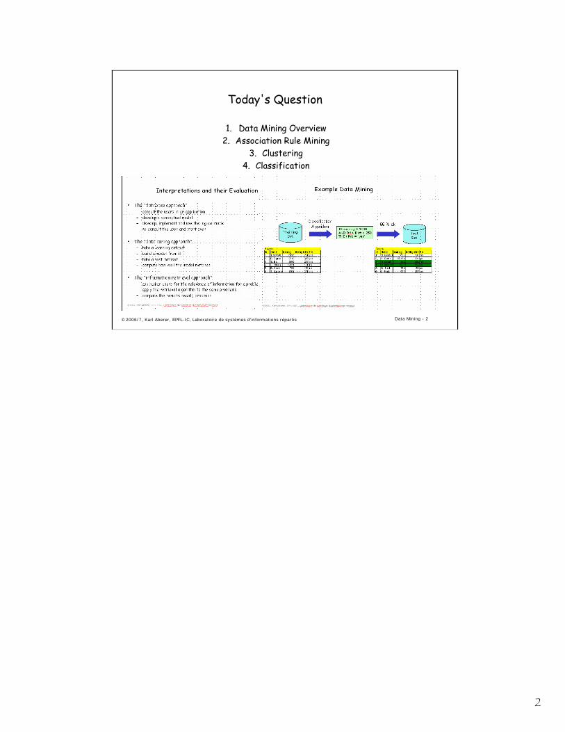
Today's Question

1. Data Mining Overview2. Association Rule Mining

3. Clustering4. Classification

3


1. Data Mining Overview

• Data acquisition and data storage result in huge databases– Supermarket and credit card transactions (market analysis)– Scientific data– Web analysis (browsing behavior, advanced information retrieval)

• Definition

Data mining is the analysis of large observational data sets to find unsuspected relationships and to summarize the data in novel ways that are both understandable and useful for the data owner

• Extraction of information from data

The wide-spread use of distributed information systems leads to the construction of large data collections in business, science and on the Web. These data collections contain a wealth of information, that however needs to be discovered. Businesses can learn from their transaction data more about the behavior of their customers and therefore can improve their business by exploiting this knowledge. Science can obtain from observational data (e.g. satellite data) new insights on research questions. Web usage information can be analyzed and exploited to optimize information access. Data mining provides methods that allow to extract from large data collections unknown relationships among the data items that are useful for decision making. Thus data mining generates novel, unsuspected interpretations of data.

4


The Classical Example: Association Rule Mining

• Market basket analysis– Given a database of purchase transactions and for each transaction a list of

purchased items– Find rules that correlate a set of items occurring in a list with another set of

items

• Example– 98% of people who purchase tires and auto accessories also get automotive

services done– 60% of people who buy diapers also buy a beer– 90% of people who buy Neal Stephenson's "Snow Crash" at amazone also buy

"Cryptonomicon"– etc.

The classical example of a data mining problem is "market basket analysis". Stores gather information on what items are purchased by their customers. The hope is, by finding out what products are frequently purchased jointly (i.e. are associated with each other), being able to optimize the marketing of the products (e.g. the layout of the store) by better targeting certain groups of customers. A famous example was the discovery that people who buy diapers also frequently buy beers (probably exhausted fathers of small children). Therefore nowadays one finds frequently beer close to diapers (and of course also chips close to beer) in supermarkets. Similarly, amazon exploits this type of associations in order to propose to their customers books that are likely to match their interests.This problem was the starting point for one of the best known data mining techniques: association rule mining.

5


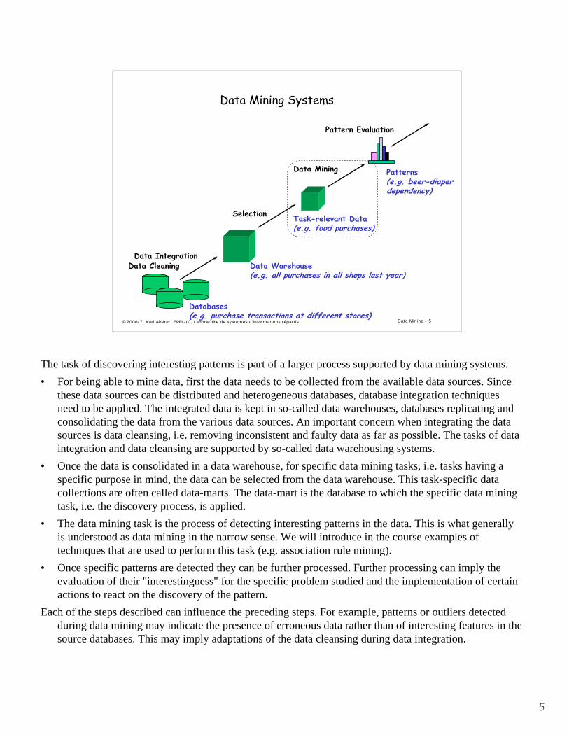
Data Mining Systems

Data CleaningData Integration

Databases (e.g. purchase transactions at different stores)

Data Warehouse (e.g. all purchases in all shops last year)

Task-relevant Data(e.g. food purchases)

Selection

Data Mining

Pattern Evaluation

Patterns(e.g. beer-diaper dependency)

The task of discovering interesting patterns is part of a larger process supported by data mining systems.• For being able to mine data, first the data needs to be collected from the available data sources. Since

these data sources can be distributed and heterogeneous databases, database integration techniques need to be applied. The integrated data is kept in so-called data warehouses, databases replicating and consolidating the data from the various data sources. An important concern when integrating the data sources is data cleansing, i.e. removing inconsistent and faulty data as far as possible. The tasks of data integration and data cleansing are supported by so-called data warehousing systems.

• Once the data is consolidated in a data warehouse, for specific data mining tasks, i.e. tasks having a specific purpose in mind, the data can be selected from the data warehouse. This task-specific data collections are often called data-marts. The data-mart is the database to which the specific data mining task, i.e. the discovery process, is applied.

• The data mining task is the process of detecting interesting patterns in the data. This is what generally is understood as data mining in the narrow sense. We will introduce in the course examples of techniques that are used to perform this task (e.g. association rule mining).

• Once specific patterns are detected they can be further processed. Further processing can imply the evaluation of their "interestingness" for the specific problem studied and the implementation of certain actions to react on the discovery of the pattern.

Each of the steps described can influence the preceding steps. For example, patterns or outliers detected during data mining may indicate the presence of erroneous data rather than of interesting features in the source databases. This may imply adaptations of the data cleansing during data integration.

6


Data Mining Techniques

Discovering Patterns and Rules"customers who by diapers buy also beer"

Descriptive ModellingGlobal description of the data

"we have three types of customers"

Predictive ModellingBuild a global function to predict values

for unknown variables from values ofknown variables

"male customers buying diapers buy beer, whereas female don't"

Retrieval by Content Find data that is similar to a pattern

Exploratory Data AnalysisNo idea what looking for

Interactive and visual tools

Local

Global

Data mining techniques can be classified according to the goals they pursue and the results they provide. A basic distinction is made among techniques that provide a global statement on the data, in the form of summaries and globally applicable rules, or that provide local statements only, in the form of rare patterns or exceptional dependencies in the data.The example of association rule mining is a typical case of discovering local patterns. The rules obtained are unexpected (unprobable) patterns and typically relate to small parts of the database only.Techniques for providing global statements on the data are further distinguished into techniques that are used to "simply" describe the data and into techniques that allow to make predictions on data if partial data is known. Descriptive modeling techniques provide compact summaries of the databases, for example, by identifying clusters of similar data items. Predictive modeling techniques provide globally applicable rules for the database, for example, allowing to predict properties of data items, if some of their properties are known.Information retrieval is usually also considered as a special case of data mining, where given patterns are searched for in the database. Finally, exploratory data analysis is used when no clear idea exists, what is being sought for in the database. It may serve as a preprocessing step for more specific data mining tasks.

7


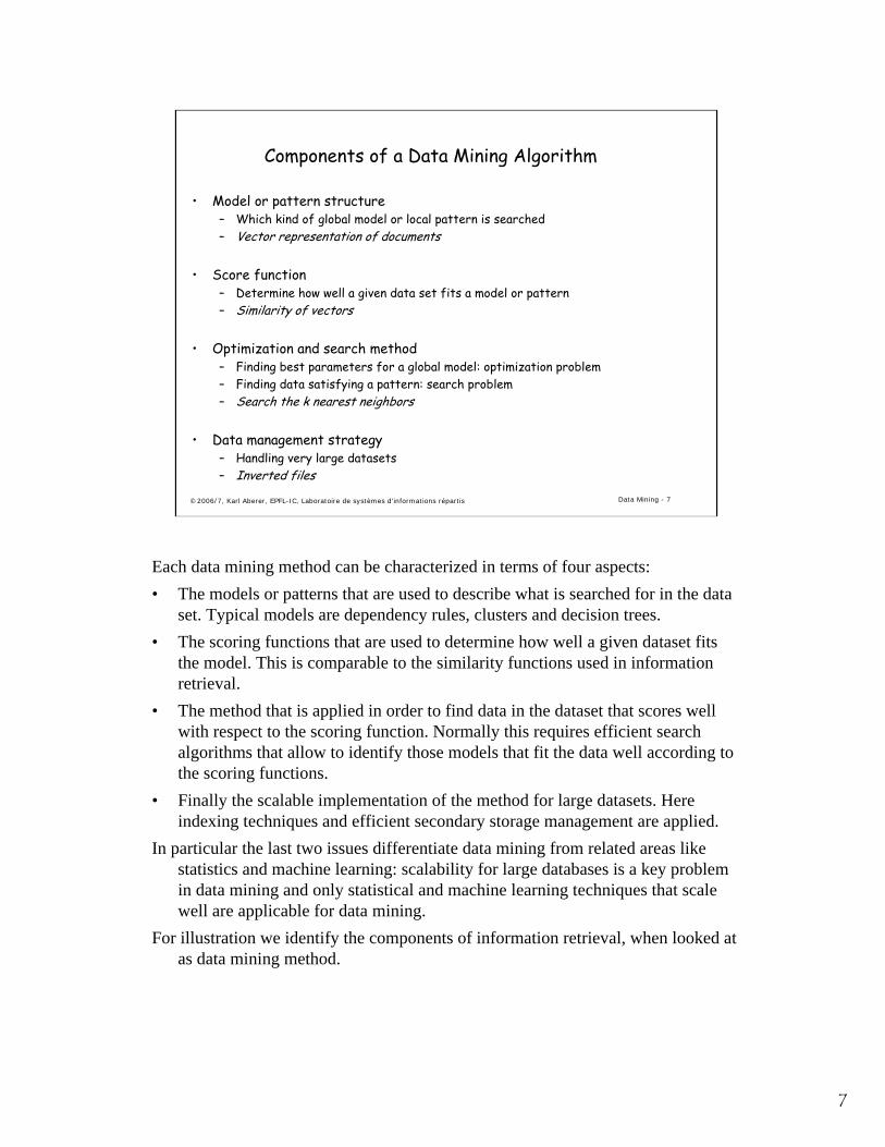
Components of a Data Mining Algorithm

• Model or pattern structure– Which kind of global model or local pattern is searched– Vector representation of documents

• Score function– Determine how well a given data set fits a model or pattern– Similarity of vectors

• Optimization and search method– Finding best parameters for a global model: optimization problem– Finding data satisfying a pattern: search problem– Search the k nearest neighbors

• Data management strategy– Handling very large datasets– Inverted files

Each data mining method can be characterized in terms of four aspects:• The models or patterns that are used to describe what is searched for in the data

set. Typical models are dependency rules, clusters and decision trees.• The scoring functions that are used to determine how well a given dataset fits

the model. This is comparable to the similarity functions used in information retrieval.

• The method that is applied in order to find data in the dataset that scores well with respect to the scoring function. Normally this requires efficient search algorithms that allow to identify those models that fit the data well according to the scoring functions.

• Finally the scalable implementation of the method for large datasets. Here indexing techniques and efficient secondary storage management are applied.

In particular the last two issues differentiate data mining from related areas like statistics and machine learning: scalability for large databases is a key problem in data mining and only statistical and machine learning techniques that scale well are applicable for data mining.

For illustration we identify the components of information retrieval, when looked at as data mining method.

8


Summary

• What is the purpose of data mining ?

• Which preprocessing steps are required for a data mining task ?

• Which are the four aspects that characterize a data mining method ?

• What is the difference between classification and prediction ?

• Explain of how information retrieval can be characterized as a data mining method ?

9


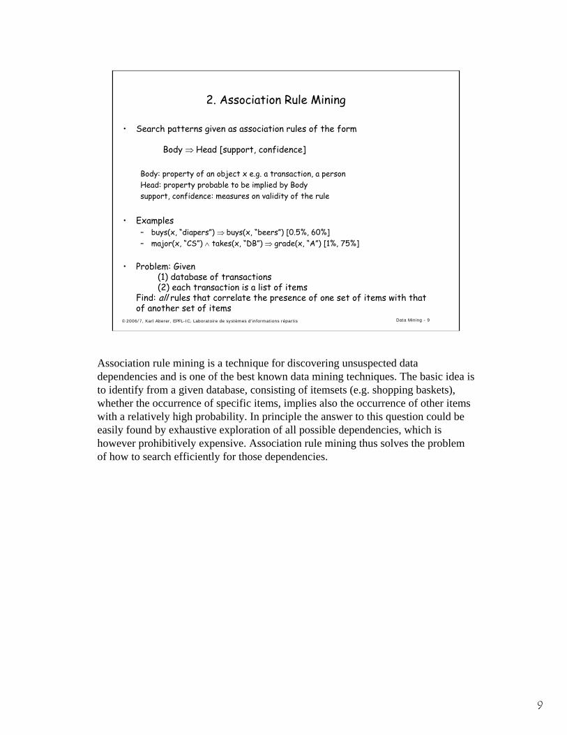
2. Association Rule Mining

• Search patterns given as association rules of the form

Body ⇒ Head [support, confidence]

Body: property of an object x e.g. a transaction, a personHead: property probable to be implied by Bodysupport, confidence: measures on validity of the rule

• Examples – buys(x, “diapers”) ⇒ buys(x, “beers”) [0.5%, 60%]– major(x, “CS”) ∧ takes(x, “DB”) ⇒ grade(x, “A”) [1%, 75%]

• Problem: Given(1) database of transactions(2) each transaction is a list of items

Find: all rules that correlate the presence of one set of items with that of another set of items

Association rule mining is a technique for discovering unsuspected data dependencies and is one of the best known data mining techniques. The basic idea is to identify from a given database, consisting of itemsets (e.g. shopping baskets), whether the occurrence of specific items, implies also the occurrence of other items with a relatively high probability. In principle the answer to this question could be easily found by exhaustive exploration of all possible dependencies, which is however prohibitively expensive. Association rule mining thus solves the problem of how to search efficiently for those dependencies.

10


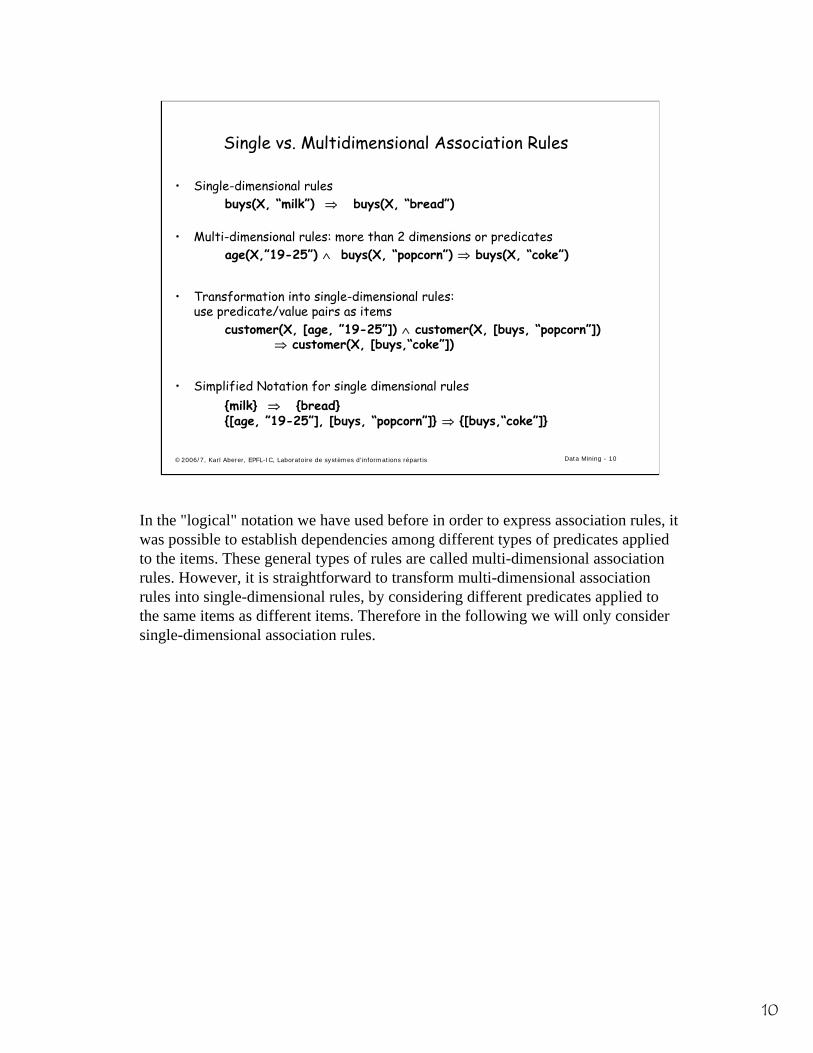
Single vs. Multidimensional Association Rules

• Single-dimensional rulesbuys(X, “milk”) ⇒ buys(X, “bread”)

• Multi-dimensional rules: more than 2 dimensions or predicatesage(X,”19-25”) ∧ buys(X, “popcorn”) ⇒ buys(X, “coke”)

• Transformation into single-dimensional rules: use predicate/value pairs as items

customer(X, [age, ”19-25”]) ∧ customer(X, [buys, “popcorn”]) ⇒ customer(X, [buys,“coke”])

• Simplified Notation for single dimensional rules{milk} ⇒ {bread}{[age, ”19-25”], [buys, “popcorn”]} ⇒ {[buys,“coke”]}

In the "logical" notation we have used before in order to express association rules, it was possible to establish dependencies among different types of predicates applied to the items. These general types of rules are called multi-dimensional association rules. However, it is straightforward to transform multi-dimensional association rules into single-dimensional rules, by considering different predicates applied to the same items as different items. Therefore in the following we will only consider single-dimensional association rules.

11


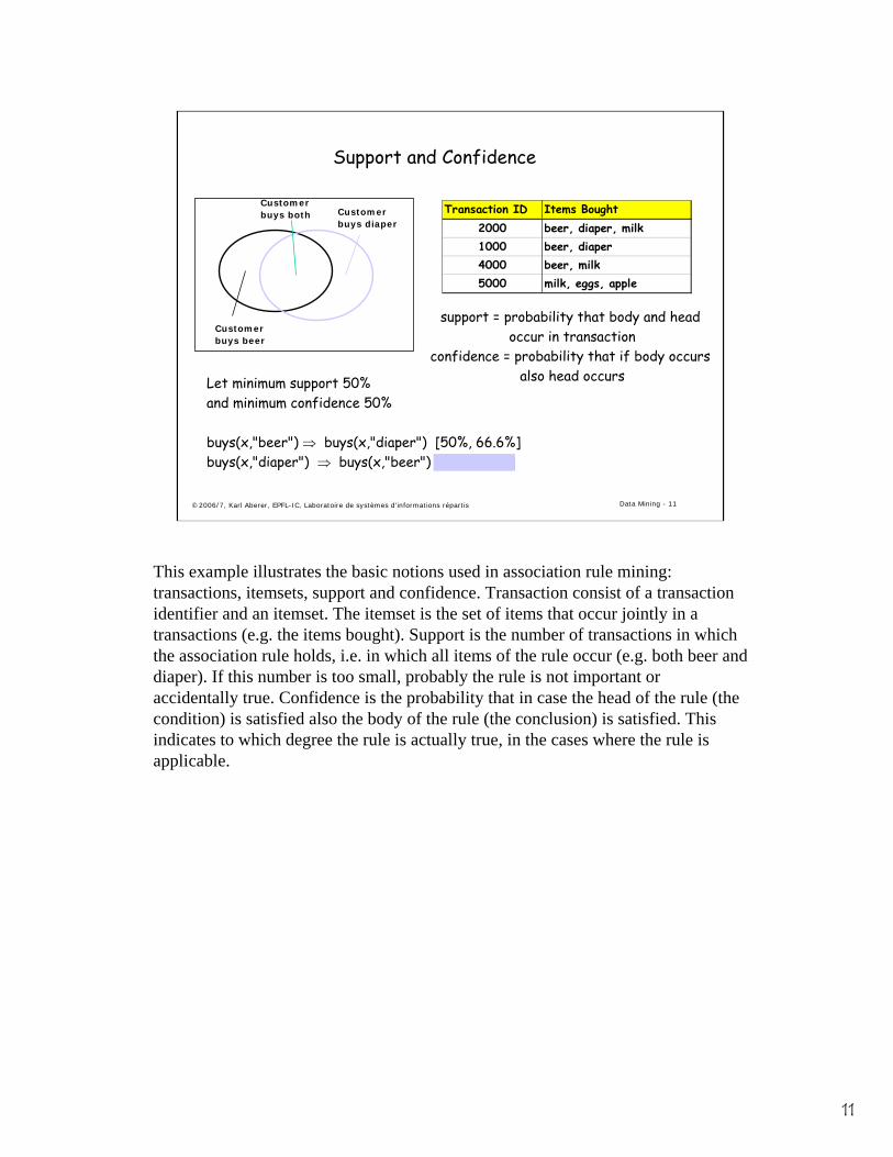
Support and Confidence

Let minimum support 50% and minimum confidence 50%

buys(x,"beer") ⇒ buys(x,"diaper") [50%, 66.6%]buys(x,"diaper") ⇒ buys(x,"beer") [50%, 100%]

Customerbuys diaper

Customerbuys both

Customerbuys beer

Transaction ID Items Bought2000 beer, diaper, milk1000 beer, diaper4000 beer, milk5000 milk, eggs, apple

support = probability that body and head occur in transaction

confidence = probability that if body occurs also head occurs

This example illustrates the basic notions used in association rule mining: transactions, itemsets, support and confidence. Transaction consist of a transaction identifier and an itemset. The itemset is the set of items that occur jointly in a transactions (e.g. the items bought). Support is the number of transactions in which the association rule holds, i.e. in which all items of the rule occur (e.g. both beer and diaper). If this number is too small, probably the rule is not important or accidentally true. Confidence is the probability that in case the head of the rule (the condition) is satisfied also the body of the rule (the conclusion) is satisfied. This indicates to which degree the rule is actually true, in the cases where the rule is applicable.

12


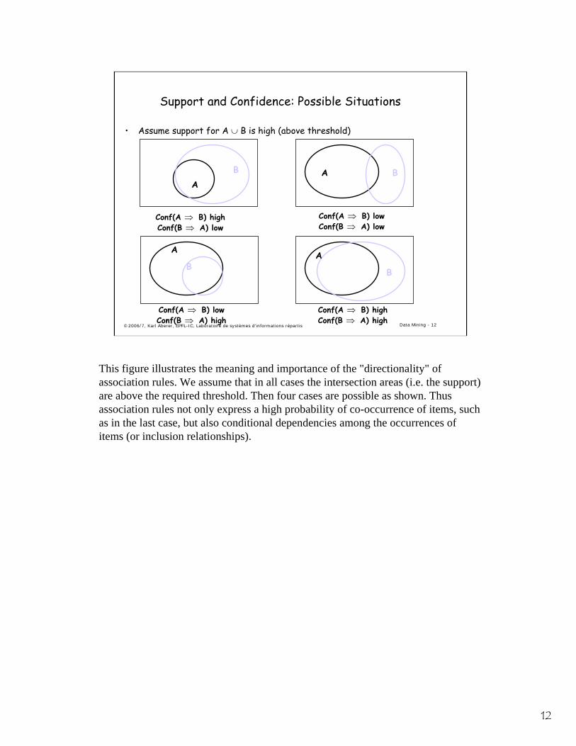
Support and Confidence: Possible Situations

• Assume support for A ∪ B is high (above threshold)

Conf(A ⇒ B) highConf(B ⇒ A) low

AB

B B

B

A A

A

Conf(A ⇒ B) lowConf(B ⇒ A) low

Conf(A ⇒ B) highConf(B ⇒ A) high

Conf(A ⇒ B) lowConf(B ⇒ A) high

This figure illustrates the meaning and importance of the "directionality" of association rules. We assume that in all cases the intersection areas (i.e. the support) are above the required threshold. Then four cases are possible as shown. Thus association rules not only express a high probability of co-occurrence of items, such as in the last case, but also conditional dependencies among the occurrences of items (or inclusion relationships).

13


Definition of Association Rules

Example: Items I = {apple, beer, diaper, eggs, milk}Transaction (2000, {beer, diaper, milk})Association rule {beer} ⇒ {diaper} [0.5, 0.66]

Terminology and NotationSet of all items I, subset of I is called itemsetTransaction (tid, T), T ⊆ I itemset, transaction identifier tidSet of all transactions D (database), Transaction T ∈ D

Definition of Association Rules A ⇒ B [s, c]A, B itemsets (A, B ⊆ I)A ∩ B emptysupport s = probability that a transaction contains A ∪ B

= P(A ∪ B)confidence c = conditional probability that a transaction having A

also contains B = P(B|A)

This is a summary of the basic notations and notions used in association rule mining.

14


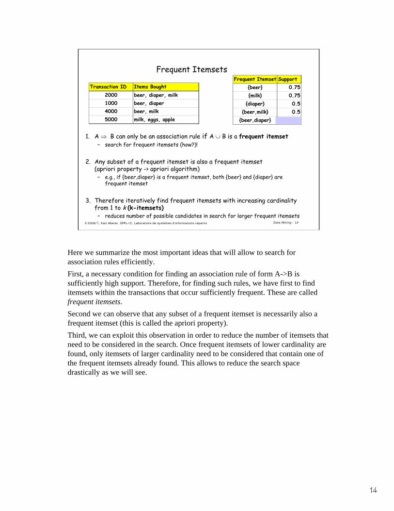
Frequent Itemsets

1. A ⇒ B can only be an association rule if A ∪ B is a frequent itemset– search for frequent itemsets (how?)!

2. Any subset of a frequent itemset is also a frequent itemset(apriori property -> apriori algorithm)– e.g., if {beer,diaper} is a frequent itemset, both {beer} and {diaper} are

frequent itemset

3. Therefore iteratively find frequent itemsets with increasing cardinality from 1 to k (k-itemsets)– reduces number of possible candidates in search for larger frequent itemsets

Transaction ID Items Bought2000 beer, diaper, milk1000 beer, diaper4000 beer, milk5000 milk, eggs, apple

Frequent Itemset Support{beer} 0.75{milk} 0.75

{diaper} 0.5{beer,milk} 0.5

{beer,diaper} 0.5

Here we summarize the most important ideas that will allow to search for association rules efficiently.First, a necessary condition for finding an association rule of form A->B is sufficiently high support. Therefore, for finding such rules, we have first to find itemsets within the transactions that occur sufficiently frequent. These are called frequent itemsets. Second we can observe that any subset of a frequent itemset is necessarily also a frequent itemset (this is called the apriori property). Third, we can exploit this observation in order to reduce the number of itemsets that need to be considered in the search. Once frequent itemsets of lower cardinality are found, only itemsets of larger cardinality need to be considered that contain one of the frequent itemsets already found. This allows to reduce the search space drastically as we will see.

15


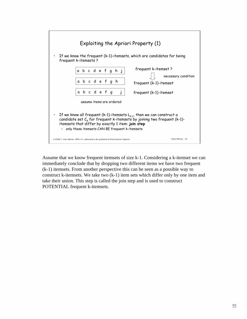
Exploiting the Apriori Property (1)

• If we know the frequent (k-1)-itemsets, which are candidates for being frequent k-itemsets ?

• If we know all frequent (k-1)-itemsets Lk-1, then we can construct a candidate set Ck for frequent k-itemsets by joining two frequent (k-1)-itemsets that differ by exactly 1 item: join step– only these itemsets CAN BE frequent k-itemsets

a b c d e f g h j

a b c d e f g h

a b c d e f g j

frequent k-itemset ?

frequent (k-1)-itemset

frequent (k-1)-itemset

necessary condition

assume items are ordered

Assume that we know frequent itemsets of size k-1. Considering a k-itemset we can immediately conclude that by dropping two different items we have two frequent (k-1) itemsets. From another perspective this can be seen as a possible way to construct k-itemsets. We take two (k-1) item sets which differ only by one item and take their union. This step is called the join step and is used to construct POTENTIAL frequent k-itemsets.

16


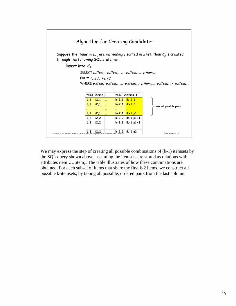
Algorithm for Creating Candidates

• Suppose the items in Lk-1 are increasingly sorted in a list, then Ck is created through the following SQL statement

insert into Ck

SELECT p.item1, p.item2, …, p.itemk-1, q.itemk-1

FROM Lk-1 p, Lk-1 qWHERE p.item1=q.item1, …, p.itemk-2=q.itemk-2, p.itemk-1 < q.itemk-1

item1 item2 … itemk-2 itemk-1i1,1 i2,1 … ik-2,1 ik-1,1i1,1 i2,1 … ik-2,1 ik-1,2… … … … …i1,1 i2,1 … ik-2,1 ik-1,p1i1,2 i2,2 ik-2,2 ik-1,p1+1i1,2 i2,2 ik-2,2 ik-1,p1+2… … … … …i1,2 i2,2 ik-2,2 ik-1,p2

take all possible pairs

We may express the step of creating all possible combinations of (k-1) itemsets by the SQL query shown above, assuming the itemsets are stored as relations with attributes item1,…,itemk. The table illustrates of how these combinations are obtained. For each subset of items that share the first k-2 items, we construct all possible k-itemsets, by taking all possible, ordered pairs from the last column.

17


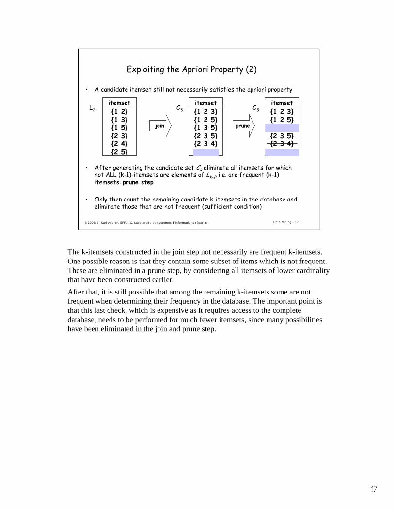
Exploiting the Apriori Property (2)

• A candidate itemset still not necessarily satisfies the apriori property

• After generating the candidate set Ck eliminate all itemsets for which not ALL (k-1)-itemsets are elements of Lk-1, i.e. are frequent (k-1) itemsets: prune step

• Only then count the remaining candidate k-itemsets in the database and eliminate those that are not frequent (sufficient condition)

L2 C3 {1 2 3}{1 2 5}{1 3 5}{2 3 5}{2 3 4}{2 4 5}

itemset{1 2}{1 3}{1 5}{2 3}{2 4}{2 5}

itemset

join prune

C3 {1 2 3}{1 2 5}{1 3 5}{2 3 5}{2 3 4}{2 4 5}

itemset

The k-itemsets constructed in the join step not necessarily are frequent k-itemsets. One possible reason is that they contain some subset of items which is not frequent. These are eliminated in a prune step, by considering all itemsets of lower cardinality that have been constructed earlier.After that, it is still possible that among the remaining k-itemsets some are not frequent when determining their frequency in the database. The important point is that this last check, which is expensive as it requires access to the complete database, needs to be performed for much fewer itemsets, since many possibilities have been eliminated in the join and prune step.

18


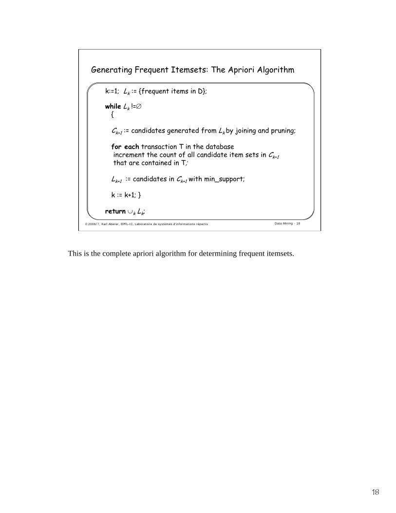
Generating Frequent Itemsets: The Apriori Algorithm

k:=1; Lk := {frequent items in D};

while Lk !=∅{

Ck+1 := candidates generated from Lk by joining and pruning;

for each transaction T in the databaseincrement the count of all candidate item sets in Ck+1that are contained in T;

Lk+1 := candidates in Ck+1 with min_support;

k := k+1; }

return ∪k Lk;

This is the complete apriori algorithm for determining frequent itemsets.

19


Example

TID Items100 1 3 4200 2 3 5300 1 2 3 5400 2 5

Database Ditemset sup.

{1} 2{2} 3{3} 3{4} 1{5} 3

itemset sup.{1} 2{2} 3{3} 3{5} 3

Scan D

C1 L1

itemset{1 2}{1 3}{1 5}{2 3}{2 5}{3 5}

itemset sup{1 2} 1{1 3} 2{1 5} 1{2 3} 2{2 5} 3{3 5} 2

itemset sup{1 3} 2{2 3} 2{2 5} 3{3 5} 2

L2 C2 C2

Scan D

C3 L3

itemset{2 3 5}

Scan D itemset sup{2 3 5} 2

min_support = 2

Notice in this example of how the scan steps (when determining the frequency with respect to the database) eliminates certain items. Notice that in this example pruning does not apply.

20


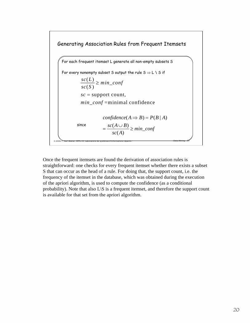
For each frequent itemset L generate all non-empty subsets S

For every nonempty subset S output the rule S ⇒ L \ S if

since

Generating Association Rules from Frequent Itemsets

( )( )

support count,=minimal confidence

sc L min_confsc Sscmin_conf

≥

=

( ) ( | )( )

( )

confidence A B P B Asc A B min_conf

sc A

⇒ =∪

= ≥

Once the frequent itemsets are found the derivation of association rules is straightforward: one checks for every frequent itemset whether there exists a subset S that can occur as the head of a rule. For doing that, the support count, i.e. the frequency of the itemset in the database, which was obtained during the execution of the apriori algorithm, is used to compute the confidence (as a conditional probability). Note that also L\S is a frequent itemset, and therefore the support count is available for that set from the apriori algorithm.

21


Example

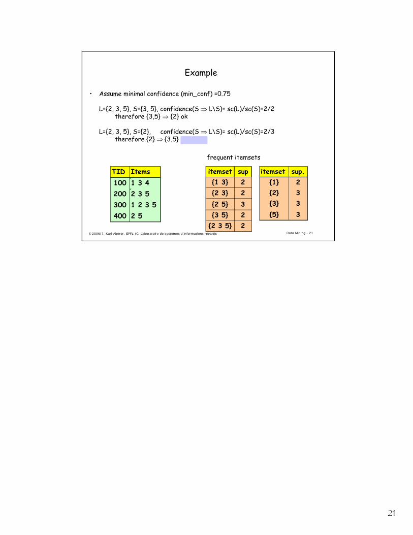
• Assume minimal confidence (min_conf) =0.75

L={2, 3, 5}, S={3, 5}, confidence(S ⇒ L\S)= sc(L)/sc(S)=2/2 therefore {3,5} ⇒ {2} ok

L={2, 3, 5}, S={2}, confidence(S ⇒ L\S)= sc(L)/sc(S)=2/3 therefore {2} ⇒ {3,5} not ok

itemset sup{1 3} 2{2 3} 2{2 5} 3{3 5} 2

{2 3 5} 2

TID Items100 1 3 4200 2 3 5300 1 2 3 5400 2 5

itemset sup.{1} 2{2} 3{3} 3{5} 3

frequent itemsets

22


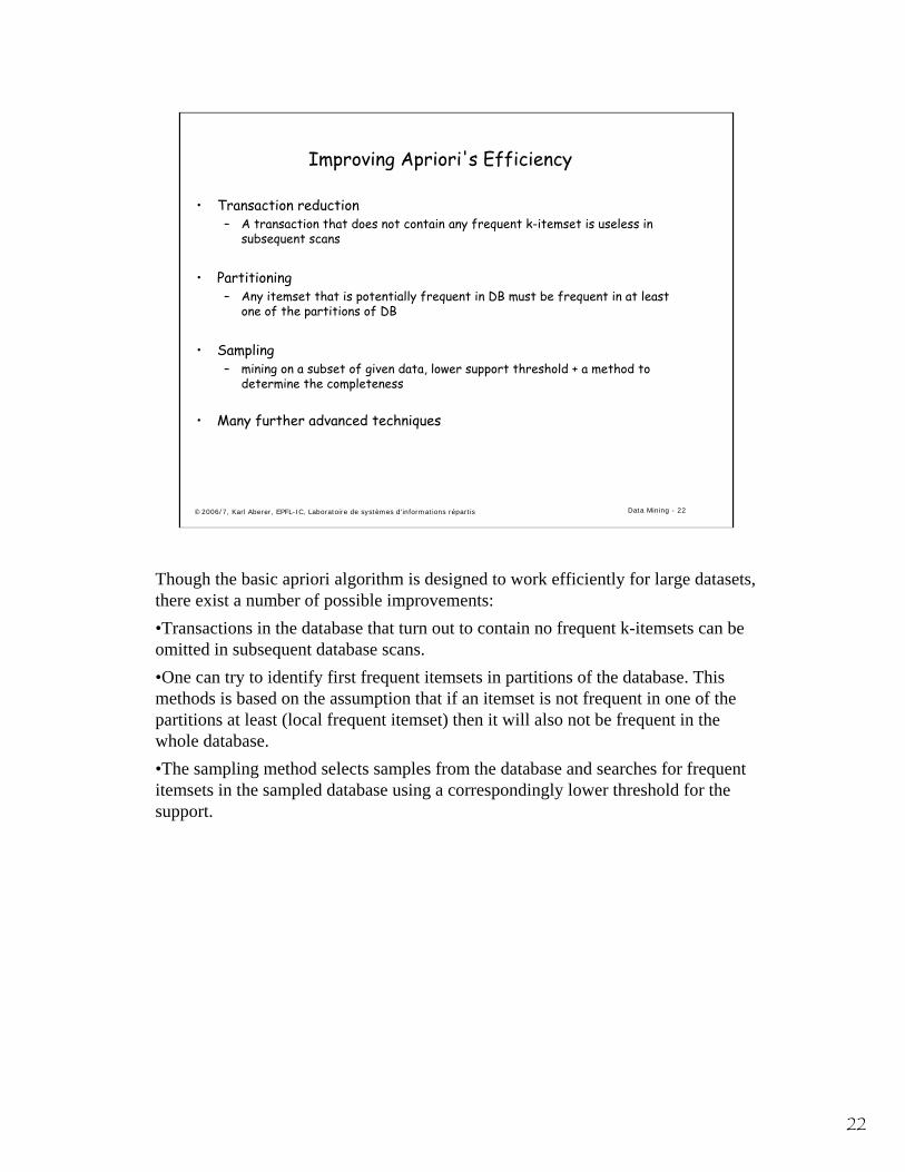
Improving Apriori's Efficiency

• Transaction reduction– A transaction that does not contain any frequent k-itemset is useless in

subsequent scans

• Partitioning– Any itemset that is potentially frequent in DB must be frequent in at least

one of the partitions of DB

• Sampling– mining on a subset of given data, lower support threshold + a method to

determine the completeness

• Many further advanced techniques

Though the basic apriori algorithm is designed to work efficiently for large datasets, there exist a number of possible improvements:•Transactions in the database that turn out to contain no frequent k-itemsets can be omitted in subsequent database scans.•One can try to identify first frequent itemsets in partitions of the database. This methods is based on the assumption that if an itemset is not frequent in one of the partitions at least (local frequent itemset) then it will also not be frequent in the whole database.•The sampling method selects samples from the database and searches for frequent itemsets in the sampled database using a correspondingly lower threshold for the support.

23


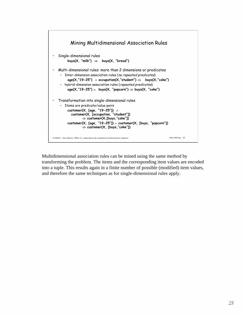
Mining Multidimensional Association Rules

• Single-dimensional rulesbuys(X, “milk”) ⇒ buys(X, “bread”)

• Multi-dimensional rules: more than 2 dimensions or predicates– Inter-dimension association rules (no repeated predicates)

age(X,”19-25”) ∧ occupation(X,“student”) ⇒ buys(X,“coke”)– hybrid-dimension association rules (repeated predicates)

age(X,”19-25”) ∧ buys(X, “popcorn”) ⇒ buys(X, “coke”)

• Transformation into single-dimensional rules– Items are predicate/value pairs

customer(X, [age, ”19-25”]) ∧customer(X, [occupation, “student”])

⇒ customer(X,[buys,“coke”])customer(X, [age, ”19-25”]) ∧ customer(X, [buys, “popcorn”])

⇒ customer(X, [buys,“coke”])

Multidimensional association rules can be mined using the same method by transforming the problem. The items and the corresponding item values are encoded into a tuple. This results again in a finite number of possible (modified) item values, and therefore the same techniques as for single-dimensional rules apply.

24


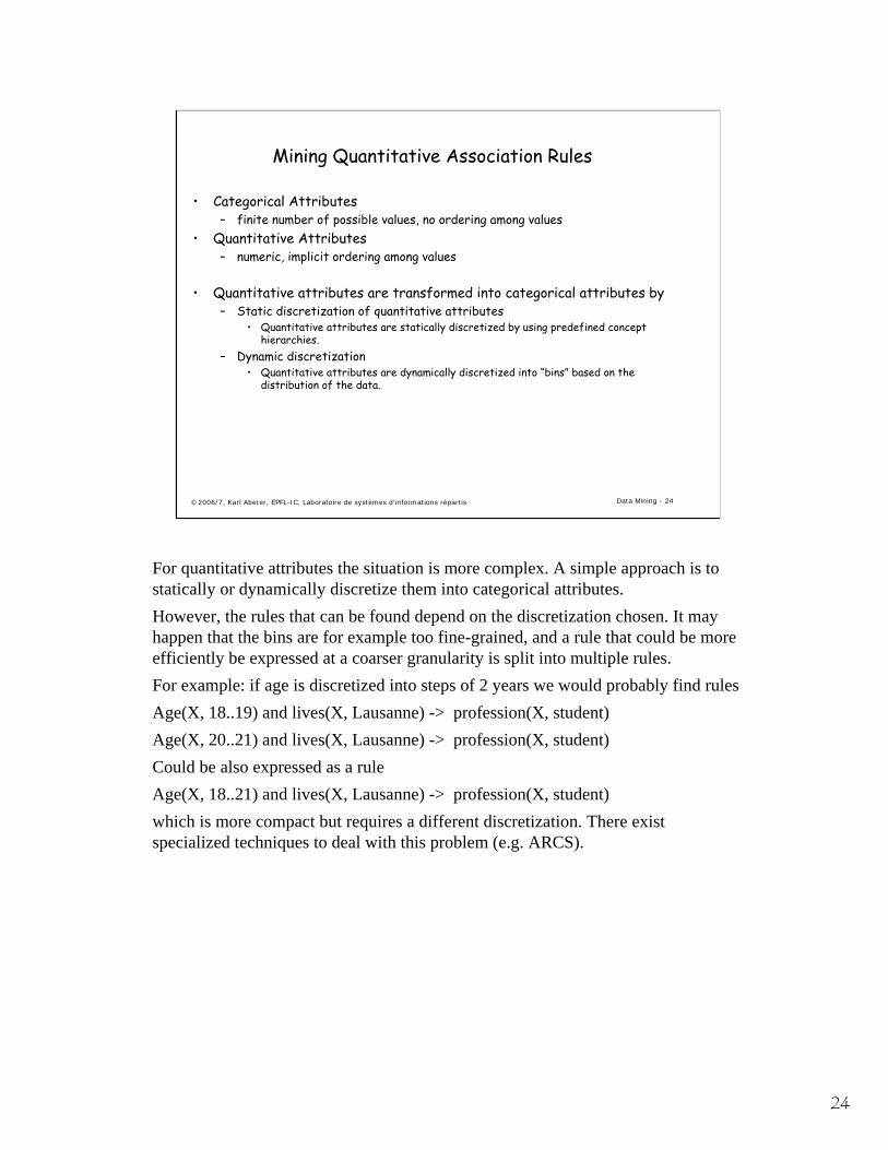
Mining Quantitative Association Rules

• Categorical Attributes– finite number of possible values, no ordering among values

• Quantitative Attributes– numeric, implicit ordering among values

• Quantitative attributes are transformed into categorical attributes by– Static discretization of quantitative attributes

• Quantitative attributes are statically discretized by using predefined concept hierarchies.

– Dynamic discretization• Quantitative attributes are dynamically discretized into “bins” based on the

distribution of the data.

For quantitative attributes the situation is more complex. A simple approach is to statically or dynamically discretize them into categorical attributes.However, the rules that can be found depend on the discretization chosen. It may happen that the bins are for example too fine-grained, and a rule that could be more efficiently be expressed at a coarser granularity is split into multiple rules.For example: if age is discretized into steps of 2 years we would probably find rulesAge(X, 18..19) and lives(X, Lausanne) -> profession(X, student)Age(X, 20..21) and lives(X, Lausanne) -> profession(X, student)Could be also expressed as a ruleAge(X, 18..21) and lives(X, Lausanne) -> profession(X, student)which is more compact but requires a different discretization. There exist specialized techniques to deal with this problem (e.g. ARCS).

25


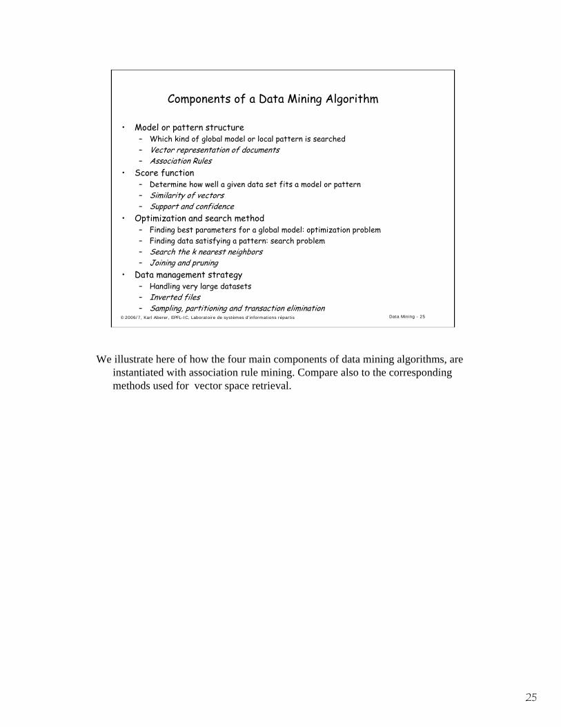
Components of a Data Mining Algorithm

• Model or pattern structure– Which kind of global model or local pattern is searched– Vector representation of documents– Association Rules

• Score function– Determine how well a given data set fits a model or pattern– Similarity of vectors– Support and confidence

• Optimization and search method– Finding best parameters for a global model: optimization problem– Finding data satisfying a pattern: search problem– Search the k nearest neighbors– Joining and pruning

• Data management strategy– Handling very large datasets– Inverted files– Sampling, partitioning and transaction elimination

We illustrate here of how the four main components of data mining algorithms, are instantiated with association rule mining. Compare also to the corresponding methods used for vector space retrieval.

26


Summary

• What is the meaning of support and confidence for an association rule ?

• Is a high support for A ∪ B a sufficient condition for A->B or B->A being an association rule ?

• Which properties on association rules and itemsets does the apriori algorithm exploit ?

• Which candidate itemsets can in the apriori algorithm be eliminated in the pruning step and which during the database scan ?

• How often is a database scanned when executing apriori ?

• How are association rules derived from frequent itemsets ?

27


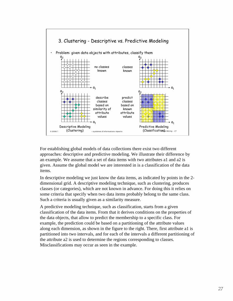
3. Clustering - Descriptive vs. Predictive Modeling

• Problem: given data objects with attributes, classify them

a1

a2

a1

a2

describeclasses

based onsimilarity of

attributevalues

a1

a2

no classesknown

Descriptive Modeling(Clustering)

classesknown

predictclasses

based onknown

attributevalues

a1

a2

Predictive Modeling(Classification)

For establishing global models of data collections there exist two different approaches: descriptive and predictive modeling. We illustrate their difference by an example. We assume that a set of data items with two attributes a1 and a2 is given. Assume the global model we are interested in is a classification of the data items. In descriptive modeling we just know the data items, as indicated by points in the 2-dimensional grid. A descriptive modeling technique, such as clustering, produces classes (or categories), which are not known in advance. For doing this it relies on some criteria that specify when two data items probably belong to the same class. Such a criteria is usually given as a similarity measure.A predictive modeling technique, such as classification, starts from a given classification of the data items. From that it derives conditions on the properties of the data objects, that allow to predict the membership to a specific class. For example, the prediction could be based on a partitioning of the attribute valuesalong each dimension, as shown in the figure to the right. There, first attribute a1 is partitioned into two intervals, and for each of the intervals a different partitioning of the attribute a2 is used to determine the regions corresponding to classes.Misclassifications may occur as seen in the example.

28


Clustering

• Model: Clusters of objects• Cluster: a collection of data objects

– Similar to one another within the same cluster– Dissimilar to the objects in other clusters

• Clustering is unsupervised classification– no predefined classes

• Typical use– As a stand-alone tool to get insight into data distribution – As a preprocessing step for other algorithms

• Typical applications– WWW

• Document classification• Cluster Weblog data to discover groups of similar access patterns

– Economic Science (especially market research)– Pattern Recognition, Spatial Data Analysis, Image Processing

Both clustering and classification aim at partitioning a dataset into subsets that bear similar characteristics. Different to classification clustering does not assume any prior knowledge, which are the classes/clusters to be searched for. There exist no class label attributes, that would tell which classes exist. Thus clustering serves in particular for exploratory data anlaysis with little or no prior knowledge.One important application of clustering we have in fact already introduced in information retrieval.The basic problem of information retrieval, i.e. find a set of documents matching a query, can be interpreted as a clustering problem, where the goal is to find two clusters of documents, namely the cluster of relevant ones and the cluster of non-relevant ones. In the tf-idf scheme in fact the tf-measure served to measure intra-cluster similarity for the two document clusters, whereas the idf-measure served to measure inter-cluster dissimilarity of the document clusters.Clustering has important applications on the Web in order to extract information from large data collections, both document collections and transactional data. Clustering is also an important tool in scientific data analysis and has, for example, a long tradition in image processing and related areas. Data mining frequently adopts techiques from these areas and extends them to make them applicable for analysing large data sets.

29


Clustering Problem

• Given: database D with N d-dimensional data items

• Find: partitioning into k clusters and noise

• A good clustering method will produce high quality clusters with– high intra-class similarity– low inter-class similarity

• The quality of a clustering result depends on both the similarity measure used by the method and its implementation

In its simplest formulation the clustering problem can be described in a way analogous to the vector space retrieval model. Given a database of data items that are represented by d-dimensional vectors (feature vectors), then partition the database into k clusters. Popular similarity measures include Euclidean distance and Manhattan distance.

30


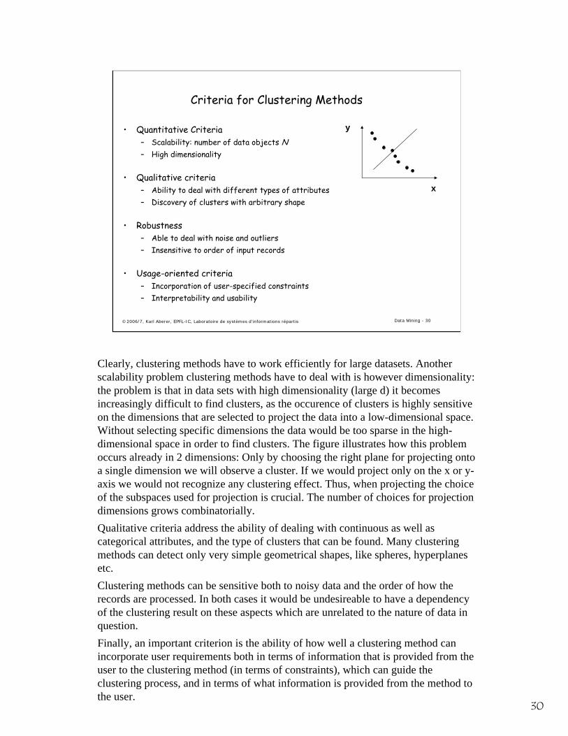
Criteria for Clustering Methods

• Quantitative Criteria– Scalability: number of data objects N– High dimensionality

• Qualitative criteria– Ability to deal with different types of attributes– Discovery of clusters with arbitrary shape

• Robustness– Able to deal with noise and outliers– Insensitive to order of input records

• Usage-oriented criteria– Incorporation of user-specified constraints– Interpretability and usability

x

y

Clearly, clustering methods have to work efficiently for large datasets. Another scalability problem clustering methods have to deal with is however dimensionality: the problem is that in data sets with high dimensionality (large d) it becomes increasingly difficult to find clusters, as the occurence of clusters is highly sensitive on the dimensions that are selected to project the data into a low-dimensional space. Without selecting specific dimensions the data would be too sparse in the high-dimensional space in order to find clusters. The figure illustrates how this problem occurs already in 2 dimensions: Only by choosing the right plane for projecting onto a single dimension we will observe a cluster. If we would project only on the x or y-axis we would not recognize any clustering effect. Thus, when projecting the choice of the subspaces used for projection is crucial. The number of choices for projection dimensions grows combinatorially.Qualitative criteria address the ability of dealing with continuous as well as categorical attributes, and the type of clusters that can be found. Many clustering methods can detect only very simple geometrical shapes, like spheres, hyperplanes etc.Clustering methods can be sensitive both to noisy data and the order of how the records are processed. In both cases it would be undesireable to have a dependency of the clustering result on these aspects which are unrelated to the nature of data in question.Finally, an important criterion is the ability of how well a clustering method can incorporate user requirements both in terms of information that is provided from the user to the clustering method (in terms of constraints), which can guide the clustering process, and in terms of what information is provided from the method to the user.

31


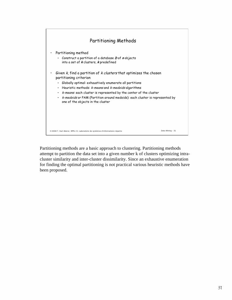
Partitioning Methods

• Partitioning method– Construct a partition of a database D of n objects

into a set of k clusters, k predefined

• Given k, find a partition of k clusters that optimizes the chosen partitioning criterion– Globally optimal: exhaustively enumerate all partitions– Heuristic methods: k-means and k-medoids algorithms– k-means: each cluster is represented by the center of the cluster– k-medoids or PAM (Partition around medoids): each cluster is represented by

one of the objects in the cluster

Partitioning methods are a basic approach to clustering. Partitioning methodsattempt to partition the data set into a given number k of clusters optimizing intra-cluster similarity and inter-cluster dissimilarity. Since an exhaustive enumerationfor finding the optimal partitioning is not practical various heuristic methods have been proposed.

32


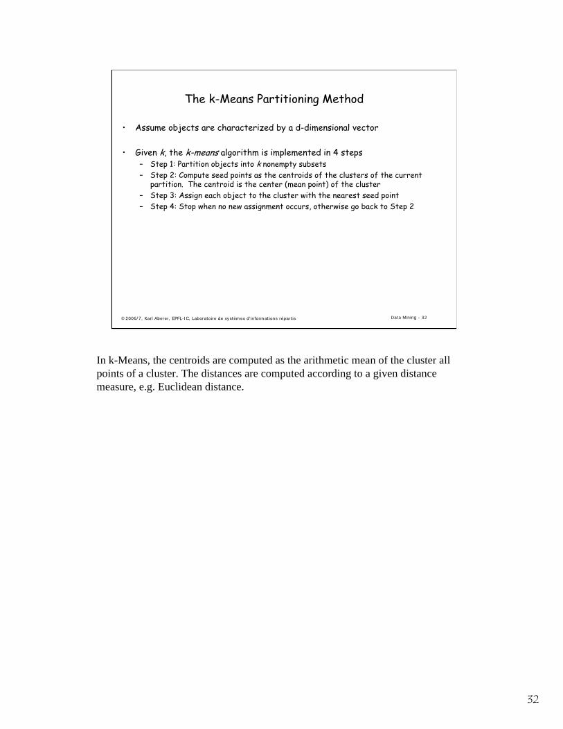
The k-Means Partitioning Method

• Assume objects are characterized by a d-dimensional vector

• Given k, the k-means algorithm is implemented in 4 steps– Step 1: Partition objects into k nonempty subsets– Step 2: Compute seed points as the centroids of the clusters of the current

partition. The centroid is the center (mean point) of the cluster– Step 3: Assign each object to the cluster with the nearest seed point– Step 4: Stop when no new assignment occurs, otherwise go back to Step 2

In k-Means, the centroids are computed as the arithmetic mean of the cluster all points of a cluster. The distances are computed according to a given distance measure, e.g. Euclidean distance.

33


Example

0

1

2

3

4

5

6

7

8

9

10

0 1 2 3 4 5 6 7 8 9 100

1

2

3

4

5

6

7

8

9

10

0 1 2 3 4 5 6 7 8 9 10

0

1

2

3

4

5

6

7

8

9

10

0 1 2 3 4 5 6 7 8 9 100

1

2

3

4

5

6

7

8

9

10

0 1 2 3 4 5 6 7 8 9 10

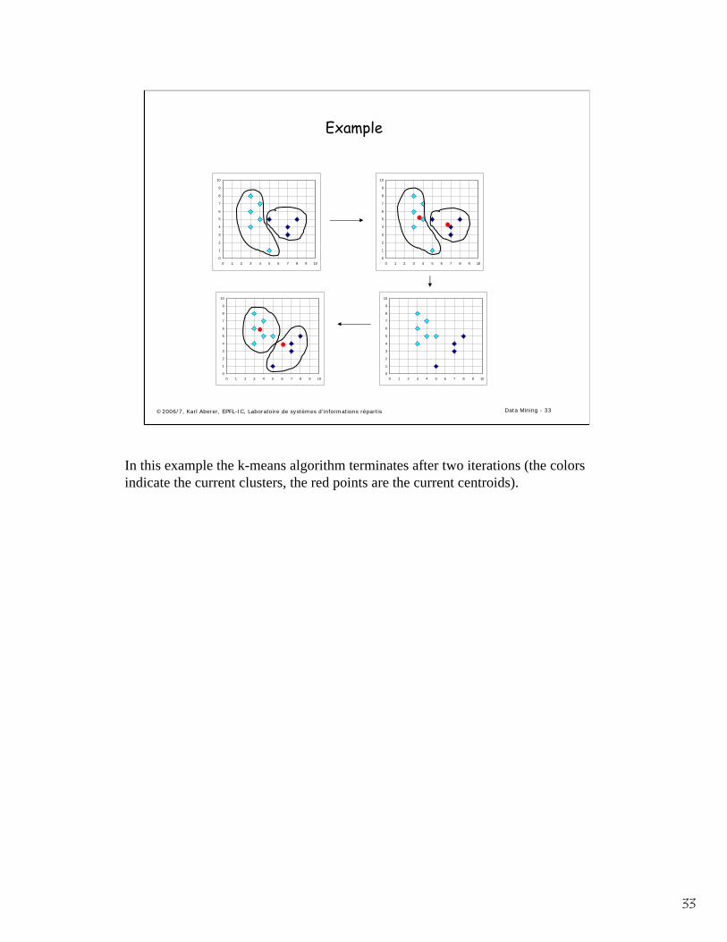
In this example the k-means algorithm terminates after two iterations (the colors indicate the current clusters, the red points are the current centroids).

34


Properties of k-Means

• Strengths– Relatively efficient: O(tkn), where n is # objects, k is # clusters, and t is #

iterations. Normally, k, t << n.– Often terminates at a local optimum, depending on seed point– The global optimum may be found using techniques such as: deterministic

annealing and genetic algorithms

• Weaknesses– Applicable only when mean is defined, therefore not applicable to categorical

data– Need to specify k, the number of clusters, in advance– Unable to handle noisy data and outliers– Not suitable to discover clusters with non-convex shapes

This assessment follows the list of criteria for evaluating clustering methods that we have introduced earlier.

35


4. Classification

• Data: tuples with multiple categorical and quantitative attributes and at least one categorical attribute (the class label attribute)

• Classification– Predicts categorical class labels– Classifies data (constructs a model) based on a training set and the values

(class labels) in a class label attribute – Uses the model in classifying new data

• Prediction/Regression– models continuous-valued functions, i.e., predicts unknown or missing values

• Typical Applications– credit approval, target marketing, medical diagnosis, treatment effectiveness

analysis

Classification creates a GLOBAL model, that is used for PREDICTING the class label of unknown data. The predicted class label is a CATEGORICAL attribute. Classification is clearly useful in many decision problems, where for a given data item a decision is to be made (which depends on the class to which the data item belongs).

36


Classification Process

• Model: describing a set of predetermined classes– Each tuple/sample is assumed to belong to a predefined class based on its

attribute values– The class is determined by the class label attribute– The set of tuples used for model construction: training set– The model is represented as classification rules, decision trees, or

mathematical formulae

• Model usage: for classifying future or unknown data– Estimate accuracy of the model using a test set – Test set is independent of training set, otherwise over-fitting will occur– The known label of the test set sample is compared with the classified result

from the model– Accuracy rate is the percentage of test set samples that are correctly

classified by the model

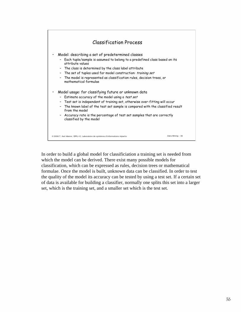
In order to build a global model for classificiation a training set is needed from which the model can be derived. There exist many possible models for classification, which can be expressed as rules, decision trees or mathematical formulae. Once the model is built, unknown data can be classified. In order to test the quality of the model its accuracy can be tested by using a test set. If a certain set of data is available for building a classifier, normally one splits this set into a larger set, which is the training set, and a smaller set which is the test set.

37


Classification: Training

TrainingSet

NAME RANK YEARS TENUREDMike Assistant Prof 3 noMary Assistant Prof 7 yesBill Professor 2 yesJim Associate Prof 7 yesDave Assistant Prof 6 noAnne Associate Prof 3 no

ClassificationAlgorithms

IF rank = ‘professor’OR years > 6THEN tenured = ‘yes’

Classifier(Model)

class label

In classification the classes are known and given by so-called class label attributes. For the given data collection TENURED would be the class label attribute. The goal of classification is to determine rules on the other attributes that allow to predict the class label attribute, as the one shown right on the bottom.

38


Classification: Model Usage

Classifier

TestSet

NAME RANK YEARS TENUREDTom Assistant Prof 2 noMerlisa Associate Prof 7 noGeorge Professor 5 yesJoseph Assistant Prof 7 yes

Unseen Data

(Jeff, Professor, 4)

Tenured?

YES

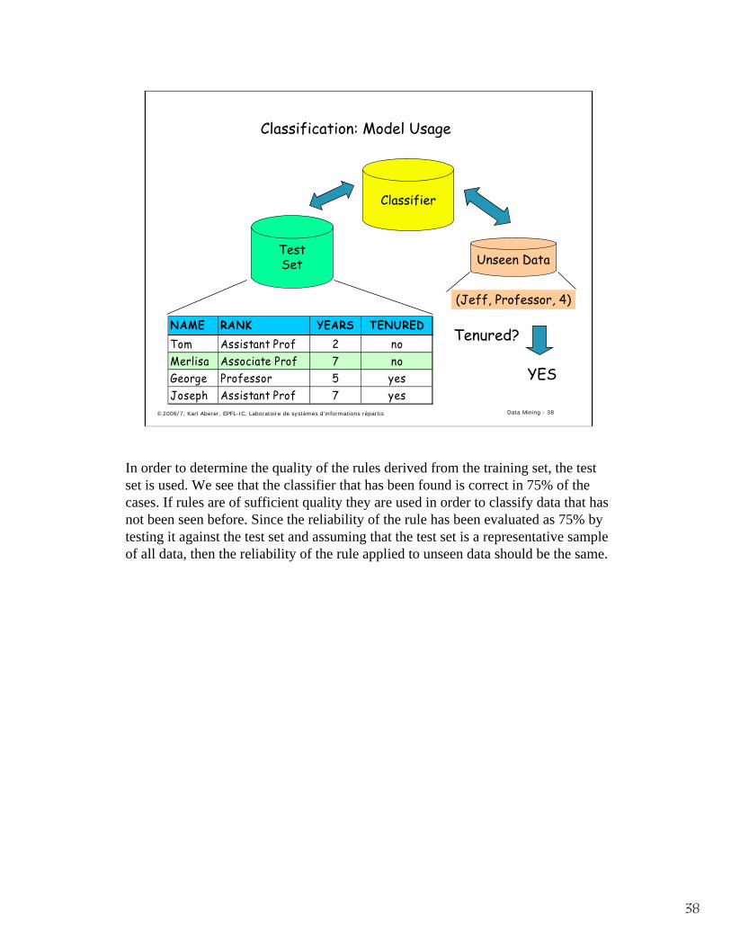
In order to determine the quality of the rules derived from the training set, the test set is used. We see that the classifier that has been found is correct in 75% of the cases. If rules are of sufficient quality they are used in order to classify data that has not been seen before. Since the reliability of the rule has been evaluated as 75% by testing it against the test set and assuming that the test set is a representative sample of all data, then the reliability of the rule applied to unseen data should be the same.

39


Criteria for Classification Methods

• Predictive accuracy

• Speed and scalability– time to construct the model– time to use the model– efficiency in disk-resident databases

• Robustness– handling noise and missing values

• Interpretability– understanding and insight provided by the model

• Goodness of rules– decision tree size– compactness of classification rules

40


Classification by Decision Tree Induction

• Decision tree – A flow-chart-like tree structure– Internal node denotes a test on a single attribute– Branch represents an outcome of the test– Leaf nodes represent class labels or class distribution

• Decision tree generation consists of two phases– Tree construction

• At start, all the training samples are at the root• Partition samples recursively based on selected attributes

– Tree pruning• Identify and remove branches that reflect noise or outliers

• Use of decision tree: Classifying an unknown sample– Test the attribute values of the sample against the decision tree

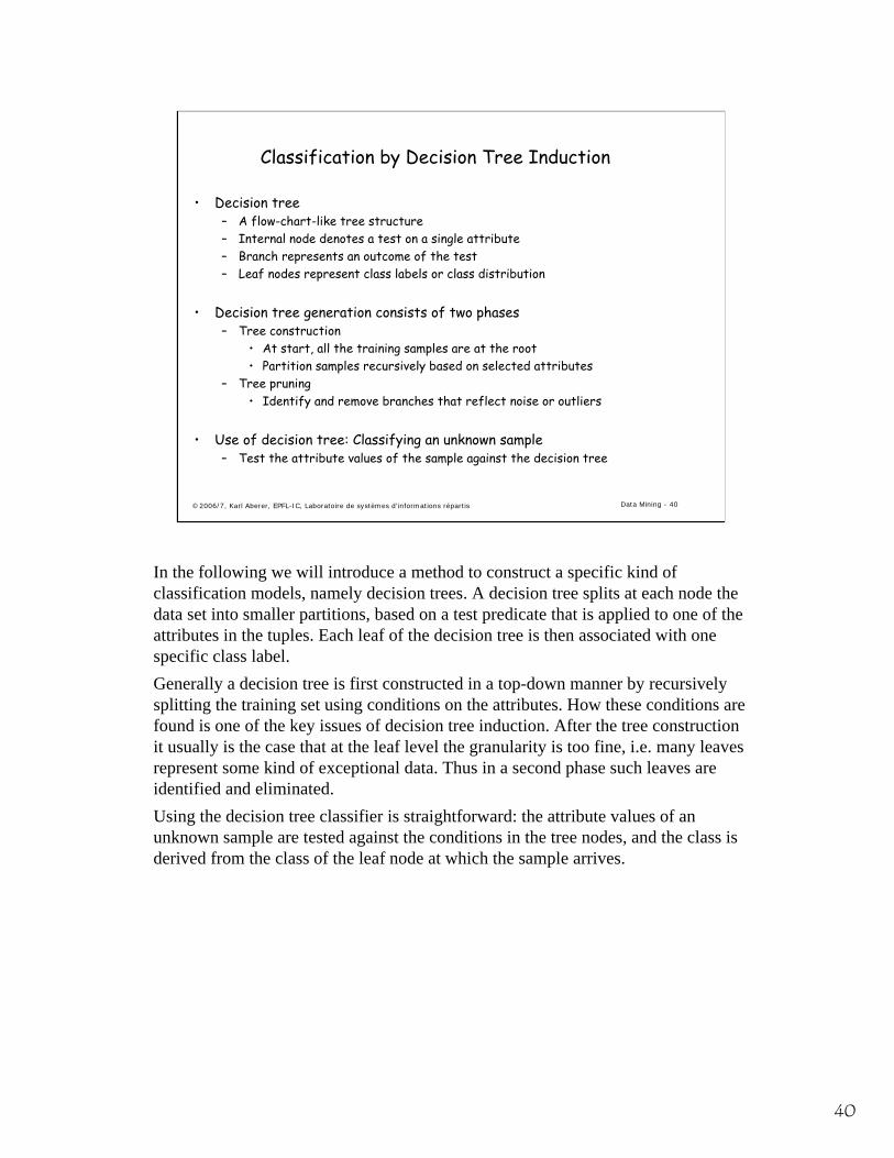
In the following we will introduce a method to construct a specific kind of classification models, namely decision trees. A decision tree splits at each node the data set into smaller partitions, based on a test predicate that is applied to one of the attributes in the tuples. Each leaf of the decision tree is then associated with one specific class label.Generally a decision tree is first constructed in a top-down manner by recursively splitting the training set using conditions on the attributes. How these conditions are found is one of the key issues of decision tree induction. After the tree construction it usually is the case that at the leaf level the granularity is too fine, i.e. many leaves represent some kind of exceptional data. Thus in a second phase such leaves are identified and eliminated.Using the decision tree classifier is straightforward: the attribute values of an unknown sample are tested against the conditions in the tree nodes, and the class is derived from the class of the leaf node at which the sample arrives.

41


Classification by Decision Tree Induction

buys_computer ?

age income student credit_rating buys_computer

<=30 high no fair no

<=30 high no excellent no

31…40 high no fair yes

>40 medium no fair yes

>40 low yes fair yes

>40 low yes excellent no

31…40 low yes excellent yes

<=30 medium no fair no

<=30 low yes fair yes

>40 medium yes fair yes

<=30 medium yes excellent yes

31…40 medium no excellent yes

31…40 high yes fair yes

>40 medium no excellent no

age?

overcast

student? credit rating?

no yes fairexcellent

<=30 >40

no noyes yes

yes

30..40

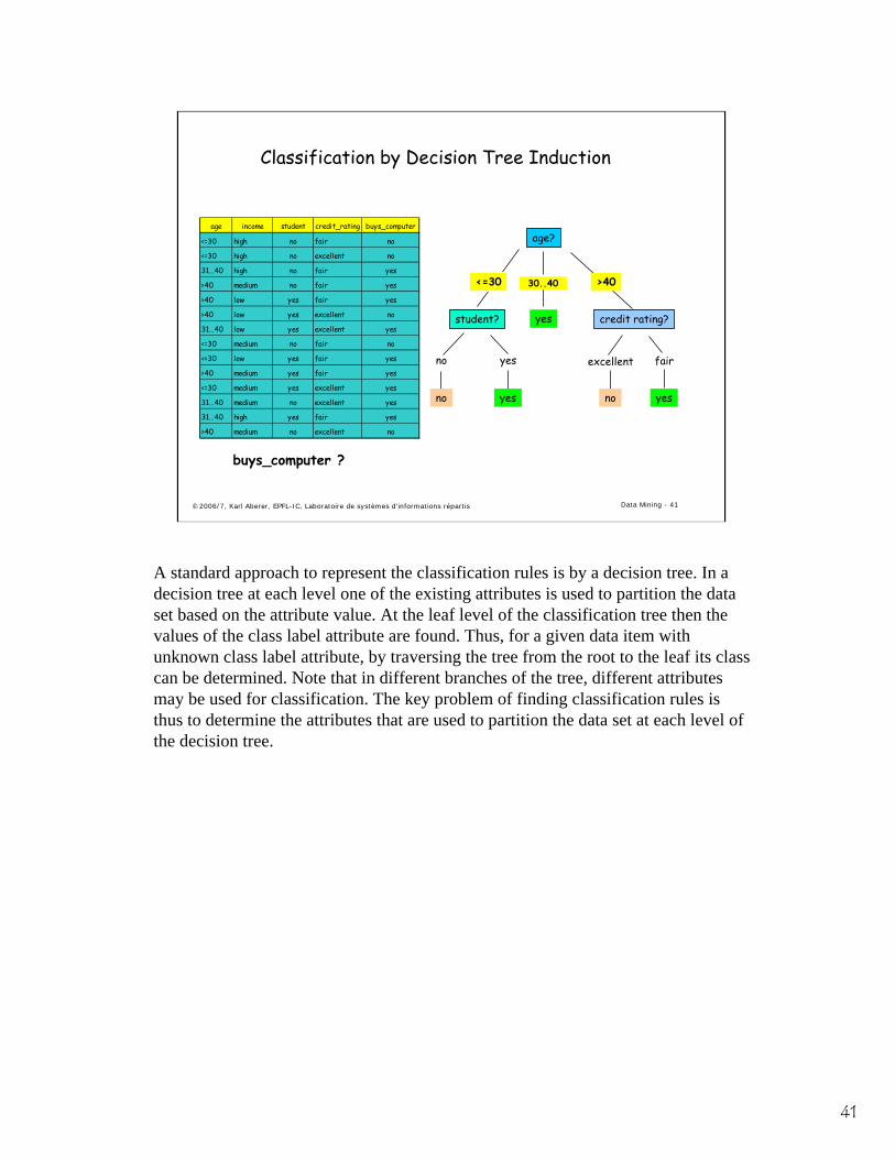
A standard approach to represent the classification rules is by a decision tree. In a decision tree at each level one of the existing attributes is used to partition the data set based on the attribute value. At the leaf level of the classification tree then the values of the class label attribute are found. Thus, for a given data item with unknown class label attribute, by traversing the tree from the root to the leaf its class can be determined. Note that in different branches of the tree, different attributes may be used for classification. The key problem of finding classification rules is thus to determine the attributes that are used to partition the data set at each level of the decision tree.

42


Algorithm for Decision Tree Construction

• Basic algorithm for categorical attributes (greedy)– Tree is constructed in a top-down recursive divide-and-conquer manner– At start, all the training samples are at the root– Examples are partitioned recursively based on test attributes– Test attributes are selected on the basis of a heuristic or statistical

measure (e.g., information gain)

• Conditions for stopping partitioning– All samples for a given node belong to the same class– There are no remaining attributes for further partitioning – majority voting

is employed for classifying the leaf– There are no samples left

• Attribute Selection Measure– Information Gain (ID3/C4.5)

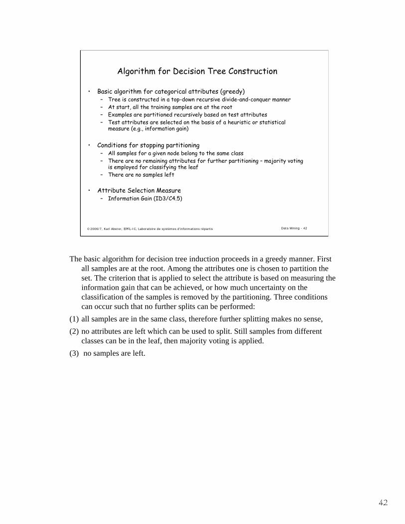
The basic algorithm for decision tree induction proceeds in a greedy manner. First all samples are at the root. Among the attributes one is chosen to partition the set. The criterion that is applied to select the attribute is based on measuring the information gain that can be achieved, or how much uncertainty on the classification of the samples is removed by the partitioning. Three conditions can occur such that no further splits can be performed:

(1) all samples are in the same class, therefore further splitting makes no sense, (2) no attributes are left which can be used to split. Still samples from different

classes can be in the leaf, then majority voting is applied.(3) no samples are left.

43


Which Attribute to Split ?

Maximize Information Gain

Class P: buys_computer = “yes”Class N: buys_computer = “no”I(p, n) = I(9, 5) =0.940 np

nnp

nnp

pnp

pnpI++

−++

−= 22 loglog),(

The amount of information, needed to decide if an arbitrary sample in S belongs to P or N

Attribute A partitions S into {S1, S2 , …, Sv} If Si contains pi examples of P and ni examples of N, the expected information needed to classify objects in all subtrees Si is

∑= +

+=

ν

1),()(

iii

ii npInpnpAE

The encoding information that would be gained by branching on A

)(),()( AEnpIAG ain −=

age pi ni I(pi, ni)<=30 2 3 0.97130…40 4 0 0>40 3 2 0.971

69.0)2,3(145

)0,4(144)3,2(

145)(

=+

+=

I

IIageE

048.0)_(151.0)(029.0)(

===

ratingcreditGainstudentGainincomeGain( ) ( , ) ( ) 0.250Gain age I p n E age= − =

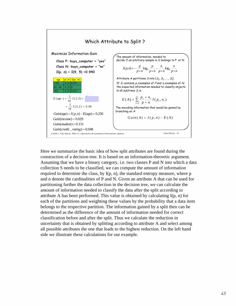
Here we summarize the basic idea of how split attributes are found during the construction of a decision tree. It is based on an information-theoretic argument. Assuming that we have a binary category, i.e. two classes P and N into which a data collection S needs to be classified, we can compute the amount of information required to determine the class, by I(p, n), the standard entropy measure, where p and n denote the cardinalities of P and N. Given an attribute A that can be used for partitioning further the data collection in the decision tree, we can calculate the amount of information needed to classify the data after the split according to attribute A has been performed. This value is obtained by calculating I(p, n) for each of the partitions and weighting these values by the probability that a data item belongs to the respective partition. The information gained by a split then can be determined as the difference of the amount of information needed for correct classification before and after the split. Thus we calculate the reduction in uncertainty that is obtained by splitting according to attribute A and select among all possible attributes the one that leads to the highest reduction. On the left hand side we illustrate these calculations for our example.

44


Pruning

• Classification reflects "noise" in the data– Remove subtrees that are overclassifying

• Apply Principle of Minimum Description Length (MDL)– Find tree that encodes the training set with minimal cost– Total encoding cost: cost(M, D)– Cost of encoding data D given a model M: cost(D | M)– Cost of encoding model M: cost(M)

cost(M, D) = cost(D | M) + cost(M)

• Measuring cost– For data: count misclassifications– For model: assume an appropriate encoding of the tree

It is important to recognize that for a test dataset a classifier may overspecialize and capture noise in the data rather than general properties. One possiblity to limit overspecialization would be to stop the partitioning of tree nodes when some criteria is met (e.g. number of samples assigned to the leaf node). However, in general it is difficult to find a suitable criterion. Another alternative is to first built the fully grown classification tree, and then in a second phase prune those subtrees that do not contribute to an efficient classification scheme. Efficiency can be measured in that case as follows: if the effort in order to specify a class (the implicit description of the class extension) exceeds the effort to enumerate all class members (the explicit description of the class extension), then the subtree is overclassifying and non-optimal. This is called the priniciple of minimum description length. To measure the description cost a suitable metrics for the encoding cost, both for trees and data sets is required. For trees this can be done by suitably counting the various structural elements needed to encode the tree (nodes, test predicates), whereas for explicit classification, it is sufficient to count the number of misclassifications that occur in a tree node.

45


Extracting Classification Rules from Trees

• Represent the knowledge in the form of IF-THEN rules– One rule is created for each path from the root to a leaf– Each attribute-value pair along a path forms a conjunction– The leaf node holds the class prediction

• Rules are easier for humans to understand

• ExampleIF age = “<=30” AND student = “no”

THEN buys_computer = “no”IF age = “<=30” AND student = “yes”

THEN buys_computer = “yes”IF age = “31…40”

THEN buys_computer = “yes”IF age = “>40” AND credit_rating = “excellent”

THEN buys_computer = “yes”IF age = “>40” AND credit_rating = “fair”

THEN buys_computer = “no”

A decision tree can also be seen as an implicit description of classification rules. Classification rules represent the classification knowledge as IF-THEN rules and are easier to understand for human users. They can be easily extracted from the classification tree as described.

46


Decision Tree Construction with Continuous Attributes

• Binary decision trees– For continuous attributes A a split is

defined by val(A) < X– For categorical attributes A a split is

defined by a subset X ⊆ domain(A)

• Determining continuous attribute splits– Sorting the data according to attribute

value– Determine the value of X which maximizes

information gain by scanning through the data items

continuous categorical class

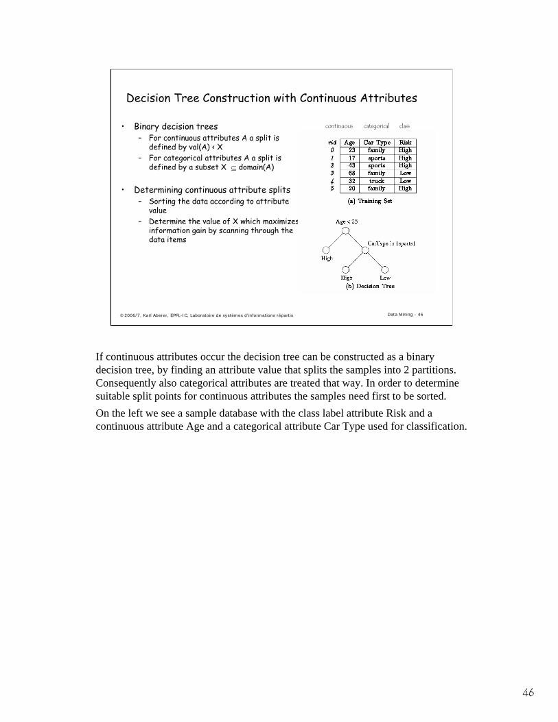
If continuous attributes occur the decision tree can be constructed as a binary decision tree, by finding an attribute value that splits the samples into 2 partitions. Consequently also categorical attributes are treated that way. In order to determine suitable split points for continuous attributes the samples need first to be sorted.On the left we see a sample database with the class label attribute Risk and a continuous attribute Age and a categorical attribute Car Type used for classification.

47


Example

I(p, n) = I(4, 2) =0.918

E(A) = 0 + ½ I(1, 2) =0.459

splitting to {sports} and {family, truck}E(A) = 0 + 2/3 I(2, 2) =0.666

Gain = I(p, n) – E(A) = 0.251

Gain = I(p, n) – E(A) = 0.459

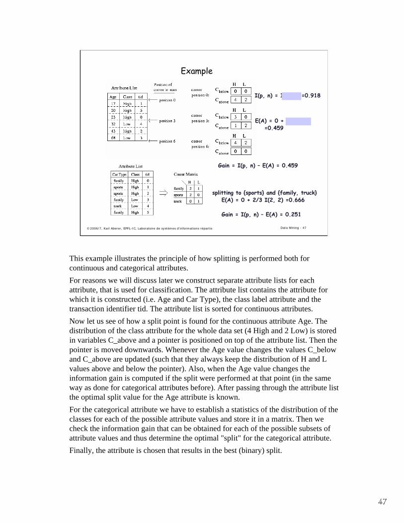
This example illustrates the principle of how splitting is performed both for continuous and categorical attributes.For reasons we will discuss later we construct separate attribute lists for each attribute, that is used for classification. The attribute list contains the attribute for which it is constructed (i.e. Age and Car Type), the class label attribute and the transaction identifier tid. The attribute list is sorted for continuous attributes. Now let us see of how a split point is found for the continuous attribute Age. The distribution of the class attribute for the whole data set (4 High and 2 Low) is stored in variables C_above and a pointer is positioned on top of the attribute list. Then the pointer is moved downwards. Whenever the Age value changes the values C_below and C_above are updated (such that they always keep the distribution of H and L values above and below the pointer). Also, when the Age value changes the information gain is computed if the split were performed at that point (in the same way as done for categorical attributes before). After passing through the attribute list the optimal split value for the Age attribute is known.For the categorical attribute we have to establish a statistics of the distribution of the classes for each of the possible attribute values and store it in a matrix. Then we check the information gain that can be obtained for each of the possible subsets of attribute values and thus determine the optimal "split" for the categorical attribute.Finally, the attribute is chosen that results in the best (binary) split.

48


Scalability

• Naive implementation– At each step the data set is split and associated with its tree node

• Problem with naive implementation– For evaluating which attribute to split data needs to be sorted according to

these attributes– Becomes dominating cost

• Idea: Presorting of data and maintaining order throughout treeconstruction– Requires separate sorted attribute tables for each attribute– Attribute selected for split: splitting attribute table straightforward– Build Hash Table associating TIDs of selected data items with partitions– Select data from other attribute tables by scanning and probing the hash

table

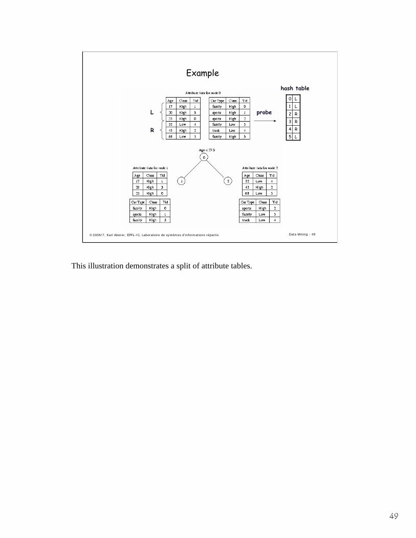
If we would associate the complete table of samples with the nodes of the classification tree during its induction, we would have to re-sort the table constantly, when searching for split points for different continuous attributes. This would become for large databases the dominating cost in the algorithm. For that reason the attribute values are stored in separate tables (as we have already seen in the example before) which are sorted once at the beginning. After a split the order in the attribute tables can be maintained:

(1) For the attribute table on which the split occurs the table needs just to be cut into two pieces.

(2) For the other tables a scan is performed, after building a hash table of the TIDs is constructed for associating the TIDs with their partition. During the scan the hash table is probed in order to redirect the tuples to their proper partition. The order of the attribute table is maintained during that process.

Remark: this is a similar idea as was employed in the construction of inverted files !

49


Example

R3

R4

L5

R2

L1

L0

probeL

R

hash table

This illustration demonstrates a split of attribute tables.

50


Summary

• What is the difference between clustering and classification ?

• What is the difference between model construction, model test and model usage in classification ?

• Which criterion is used to select an optimal attribute for partitioning a node in the decision tree ?

• How are clusters characterized ?

• When is the k-Means algorithm terminating ?

51


References

• Textbook– Jiawei Han, Data Mining: concepts and techniques, Morgan Kaufman, 2000,

ISBN 1-55860-489-8

• Some relevant research literatue– R. Agrawal, T. Imielinski, and A. Swami. Mining association rules between

sets of items in large databases. SIGMOD'93, 207-216, Washington, D.C.

52


Looking back

• Part 1: Semi-structured data management– How to model and process structured data from the Web– Model known, processing centralized

• Part 2: Distributed data management– How to process structured data in a physically distributed system– Model known, processing distributed

• Part 3: Information retrieval and data mining– How to extract models from unstructured content– Model unknown, processing centralized

• Part 4?

53


The Exam

• Date and Place: Monday, 26th of February from 14:15 – 17:15 (CO010, CO2, CO3)

• Two midterm exams and one final exam (written)– midterms contribute 25% each to final grade, if improvement

• Conceptual questions and practical problems– will assume you attended the lecture– will assume you did the programming exercises– examples from earlier years (exercises, exams) provided for preparation

• Support: Lecture Slides + Exercises + Handwritten Notes

54


… and finally

… thanks for the attention,… for all questions and observations,

and good luck for the future!

chapter 4 – data mining a short introductionlsir minin… · · 2007-02-053 ©2006/7, karl...

Documents