chapter 4 geophysical investigations -...
TRANSCRIPT
59
CHAPTER – 4
GEOPHYSICAL INVESTIGATIONS
4.1 Introduction
Electrical resistivity methods of geophysical prospecting are well established and
the most important method for groundwater investigations. The electrical resistivity
method is one that has been widely used because of the theoretical, operational and
interpretational ease. The advantages of electrical methods also include control over
depth of investigation, portability of the equipment, availability of wide range of simple
and elegant interpretation techniques, and the related software etc. Direct current (D.C.)
resistivity (electrical resistivity) techniques measure earth resistivity by driving a D.C.
signal into the ground and measuring the resulting potentials (voltages) created in the
earth. From the data obtained, the electrical properties of the earth (the geoelectric
section) can be derived. In turn, from those electrical properties we can infer the
geological characteristics of the earth.
In geophysical and geotechnical literature, the terms “electrical resistivity” and
“D.C. resistivity” are used synonymously. Several geological parameters which affect
earth resistivity (and its reciprocal, conductivity) include clay content, soil or formation
porosity and degree of water saturation.
The theory and practice of this method for groundwater investigations is well
documented by Bhattacharya and Patra (1968) and Parasinis (1973). The interpretation of
resistivity data and its application to groundwater studies has been given in detail by
Zohdy (1965 and 1975). D.C resistivity techniques may be used in the profiling mode
(Wenner surveys) to map lateral changes and identify near-vertical features or they may
be used in the sounding mode (Schlumberger array) to determine depths to geoelectric
horizons (Ex. depth to water table). Both profiling and vertical electrical sounding (VES)
has been successfully applied to various geological formations by (Flathe 1955; Ogilvy
1967; Ogilvy et al. 1980; Zohdy et al. 1974). Common applications of the D.C resistivity
method include delineation of aggregate deposits for quarry operations, estimating depth
60
to water table and bedrock or to other geoelectric boundaries, mapping and/or detecting
other geologic features (Verma et al. 1980).
4.2 Electrical properties of geological formation
The electrical resistivity of a geological formation is physical characteristic,
determines the flow of electric current in the formation. Resistivity varies with texture of
the rock nature of mineralization and conductivity of electrolyte contained within the
rock (Parkhomenko et al. 1967). Resistivity not only changes from formation to
formation but even within a particular formation (Sharma 1997). Resistivity increases
with grain size and tends to maximum when the grains are coarse (Sharma and Rao
1962), also when the rock is fine grained and compact. The resistivity drastically reduces
with increase in clay content and which are commonly dispersed throughout as coatings
on grains or disseminated masses or as thin layers or lenses. In saturated rocks, low
resistivity can be due to increased clay content or salinity. Hence, the resistivity surveys
are the best suited for delineation of clay or saline zone.
Further, combining resistivity data with insitu total dissolved solids (TDS) or
electrical conductivity measurements in wells can help identify shallow contaminated
zones. A combination of Hydrogeological, geophysical and geochemical investigations
can be very effective in the detection of contaminant migration (Sankaran et al. 2005).
Detection of contamination due to mine seepage, oil field leakage and hazardous waste
disposal were discussed by Warner 1969; Kelly 1976; Urish 1983; Mazac et al. 1987;
Ebraheem et al. 1990 and 1996 and Barker et al. 1981. Similarly, in the present study also
attempt has been made to trace the extent of pollution due to industries and anthropogenic
activities within the study area based on the resistivity methods.
4.3 Electrical Resistivity Method
In resistivity method of electrical prospecting, an electric field is artificially
created in the ground by means of either galvanic batteries (DC) or low frequency AC
generators. The energizing current is sent in to the ground by means of two grounded
electrodes, called the current electrodes designated as „A‟ and „B‟ placed at two selected
points. The potential in the area is measured by another two more grounded electrodes
61
called the potential electrodes designated as „M‟ and „N‟. Electrical resistivity is defined
as the resistance offered by a unit cube of material for the flow of current through its
normal surface. If „L‟ is the length of the conductor and „A‟ is its cross-sectional area,
then the resistance (R) is defined as
R=L/A
In MKS system the unit of resistivity is Ohm-meter(W-m). The reciprocal of
resistivity is called conductivity and denoted by σ, the unit of conductivity is mho/meter.
4.3.1 Apparent resistivity
For a homogeneous and isotropic conducting medium ρ is independent of the
position of electrodes on the surface and electrode configuration while measuring the
potential difference between any two points in a four-electrode array comprising a pair of
current and potential electrodes. Hence, it is designated as true resistivity of the medium
(Bhattacharya and Patra 1968 and Sharma 1997). For heterogeneous medium, the
resistivity is called the apparent resistivity. The apparent resistivity of geologic formation
is equal to the true resistivity of fictitious homogeneous and isotropic medium in which,
for a given electrode configuration and current strength, I, the measured potential
difference ∆V is equal to that for the given heterogeneous and anisotropic medium. The
apparent resistivity depends upon the geometry and resistivity of the elements
constituting the given geologic medium.
a = K (∆V/I)
Where K is the geometrical factor having the dimension of length (m). Resistivity
of rock formations varies over a wide range; depending on mineral constituents of rock,
density, porosity, pore size and shape, water content, quality of water and temperature.
There is no fixed limit for resistivity of various rocks; igneous and metamorphic rocks
yield values in the range of 102 to 108 Ω-m; sedimentary and unconsolidated rocks vary
between 1 to 104 Ω-m.
62
4.3.2 Resistivity measurements
Generally, for measuring the resistivities of the subsurface formations, four
electrodes namely two current electrodes A and B and two potential electrodes M and N
are required. There are different electrode arrangements for measuring the potential
difference, which are uniquely used for different purposes in exploration techniques
(Keller and Frishknecht, 1966). The most popular among them are Wenner (1915) and
Schlumberger (1920).
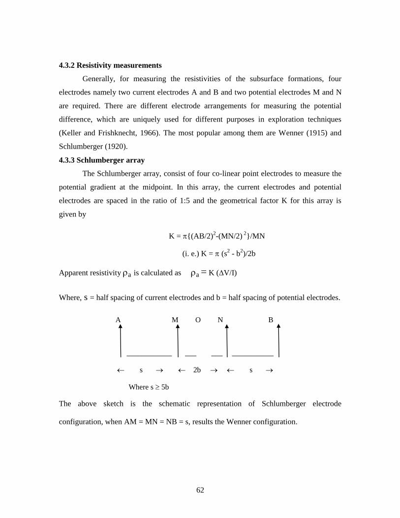
4.3.3 Schlumberger array
The Schlumberger array, consist of four co-linear point electrodes to measure the
potential gradient at the midpoint. In this array, the current electrodes and potential
electrodes are spaced in the ratio of 1:5 and the geometrical factor K for this array is
given by
K = {(AB/2)2-(MN/2)
2}/MN
(i. e.) K = (s2 - b
2)/2b
Apparent resistivity a is calculated as a = K (∆V/I)
Where, s = half spacing of current electrodes and b = half spacing of potential electrodes.
A M O N B
____________ ___ ___ ___________
s 2b s
Where s 5b
The above sketch is the schematic representation of Schlumberger electrode
configuration, when AM = MN = NB = s, results the Wenner configuration.
63
4.4 Vertical electrical sounding (VES)
Resistivity sounding is the study of resistivity variation with depth for fixed center
i.e. vertical investigations of subsurface geological layers. It is also called as vertical
electrical sounding (VES). This method gives the information about depth and thickness
of various subsurface layers and their potential for groundwater exploitation. Since the
fraction of total current flows at a depth varies with the current electrodes separations, the
field procedure is to use a fixed center with an expanding spread. The Wenner and
Schlumberger arrays are particularly suited to this technique, where in Schlumberger
array has some specific advantages. There are always some naturally developing potential
(self-potential, SP) in the ground, which have to be eliminated and nullified. Thus, in
such electrode configuration, the potential difference for a selected value of AB/2 is
measured and in turn, the festivities are obtained. The resistivities are plotted against
AB/2 on a double log graph. A log-log plot of the apparent resistivity versus current
electrode spacing (AB/2) is commonly referred to as the “sounding curve”. Resistivity
data is generally interpreted using the “modeling” process. A hypothetical model of the
earth and its resistivity structure (geoelectric section) is generated. The theoretical
electrical resistivity response over that model is then calculated and compared with the
observed field response. The differences between the observed and the calculated are
then adjusted to create a response, which very closely fits the observed data. When this
iterative process is automated, it is referred to as “iterative inversion” or “optimization”.
The product from a D.C resistivity survey or VES is generally a “geoelectric”
cross section showing thickness and resistivities of all the geoelectric units or layers. If
borehole data or a conceptual geologic model is available, then a geologic identity can be
assigned to the geoelectric units. A two dimensional geoelectric section may be made up
of a series of one-dimensional soundings joined together, which yield the required
subsurface information.
4.5 Multi-electrode resistivity imaging (MERI)
The improvement of resistivity methods using multi-electrode arrays has led to an
important growth of electrical imaging for subsurface surveys (Griffith et al. 1990;
Griffith and Barker 1993). The multi-electrode resistivity technique is now fairly well
64
established with respect to theory, practical application and interpretation techniques
(Barker 1981; Dahlin 1993; Loke and Barker 1996a, 1996b). Electrical sounding (1-D
vertical) and electrical profiling (1-D lateral) are routinely used for groundwater
investigations and are well described in standard geophysical text such as Battacharya
and Patra (1968), Grant and West (1965), Dobrin (1976), Reynolds (1997), Koefoed
(1979), Maillet (1947) and Telford et al. (1990). A detail picture of the subsurface can be
obtained by combining the sounding and profiling data to give two-dimensional (2-D)
cross sections, which in turn can be combined to give a 3-D model of the ground. Multi
electrode resistivity imaging techniques (Dahlin 1993) is a combination of both sounding
and profiling which has been used as a complimentary to traditional electrical resistivity
methods in this work. Such surveys are usually carried out using a large number of
electrodes, say 24 or more, connected to a multi core cable. A laptop microcomputer
together with an electrode-switching unit is used to automatically select the relevant four
electrodes for each measurement. Apparent resistivity measurements are recorded
sequentially sweeping any quadripole (current and potential electrodes) within the multi
electrode array. As a result, high-definition pseudo sections with dense sampling of
apparent resistivity variation at shallow depth (10-100 m) are obtained in a short time. It
allows the detailed interpretation of 2-D resistivity distribution in the ground (Loke and
Barker 1996a). A resistivity meter SYSCAL Junior Switch (made in France) has been
used in the present case with 48 electrodes connected to the meter through a multi-core
cable having unit electrode spacing of 5 meters.
4.6 Field investigations
In general, electrical investigations particularly vertical electrical soundings and
multi-electrode resistivity imaging are conducted to determine the depth to Bedrock,
groundwater potential zones and sources of groundwater pollution. Some of the
significant applications are lateral differentiation of permeable formations from
impermeable or less permeable formations and vertical distribution of various layers. 25
vertical electrical soundings (VES) were carried out at selected locations within the study
area in order to decipher the subsurface conditions (Figure 4.1). The VES were carried
out using a NGRI make D.C Resistivity meter where in the current and potential readings
are displayed for calculating the resistance. Cast iron stakes as current electrodes and
65
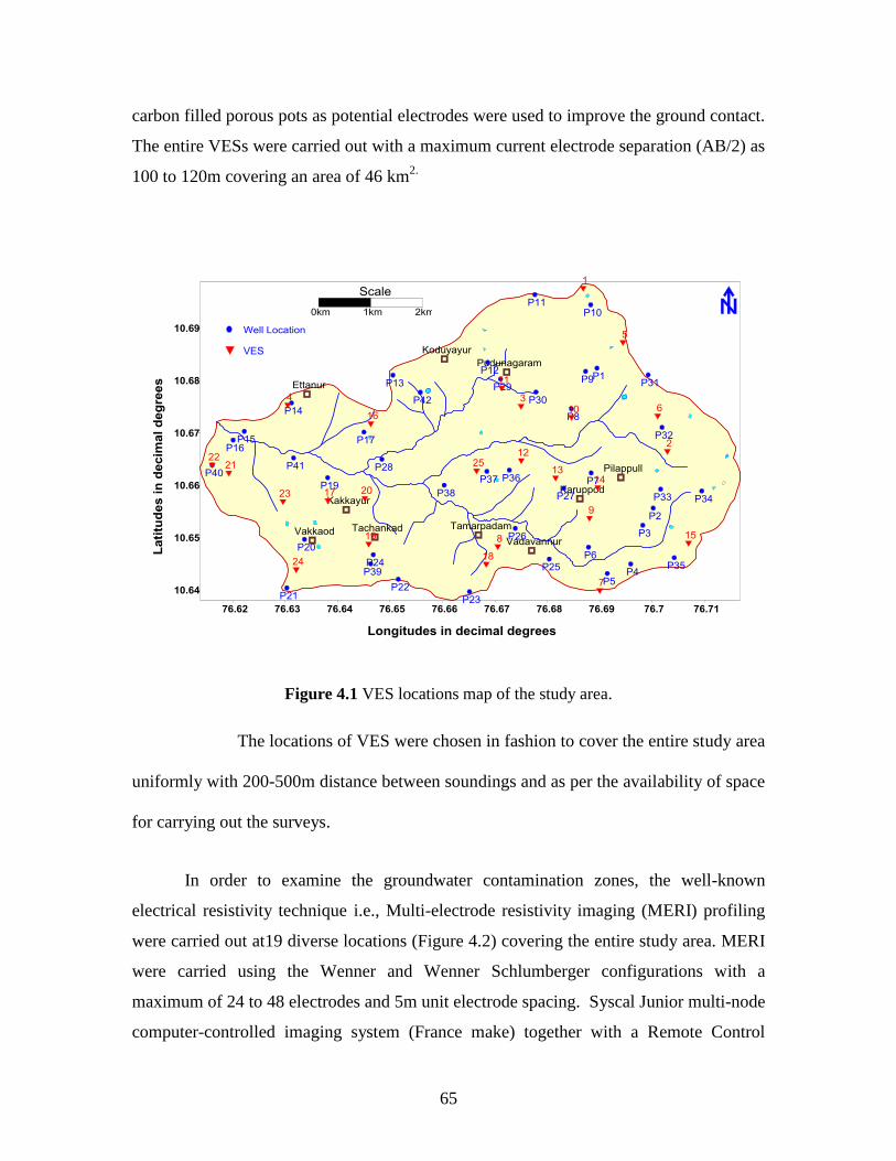
carbon filled porous pots as potential electrodes were used to improve the ground contact.
The entire VESs were carried out with a maximum current electrode separation (AB/2) as
100 to 120m covering an area of 46 km2.
Figure 4.1 VES locations map of the study area.
The locations of VES were chosen in fashion to cover the entire study area
uniformly with 200-500m distance between soundings and as per the availability of space
for carrying out the surveys.
In order to examine the groundwater contamination zones, the well-known
electrical resistivity technique i.e., Multi-electrode resistivity imaging (MERI) profiling
were carried out at19 diverse locations (Figure 4.2) covering the entire study area. MERI
were carried using the Wenner and Wenner Schlumberger configurations with a
maximum of 24 to 48 electrodes and 5m unit electrode spacing. Syscal Junior multi-node
computer-controlled imaging system (France make) together with a Remote Control
66
Module was used. All surveys were done using 0.4 m length of stainless steel electrodes,
which were planted to a depth of 0.3 m. Each electrode was watered to ensure good
contact with the ground. This was done most effectively by withdrawing the electrode
from the ground, filling the hole with water and replanting the electrode. The survey lines
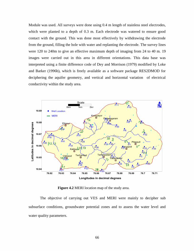
were 120 to 240m to give an effective maximum depth of imaging from 24 to 40 m. 19
images were carried out in this area in different orientations. This data base was
interpreted using a finite difference code of Dey and Morrison (1979) modified by Loke
and Barker (1996b), which is freely available as a software package RES2DMOD for
deciphering the aquifer geometry, and vertical and horizontal variation of electrical
conductivity within the study area.
Figure 4.2 MERI location map of the study area.
The objective of carrying out VES and MERI were mainly to decipher sub
subsurface conditions, groundwater potential zones and to assess the water level and
water quality parameters.
67
4.7 Interpretation procedures
4.7.1 Vertical electrical sounding (VES)
There are four basic type of sounding curve depending on the resistivity
distribution with depth. If ρ1, ρ2 and ρ
3 are the resistivity of the subsurface layers with ρ
1
at the top followed by ρ2 and ρ
3
i. ρ1 < ρ2 < ρ3 is defined as A-type
ii. ρ1 <ρ2 > ρ3 is defined as K-type
iii. ρ1 > ρ2 < ρ3 is defined as H-type
iv. ρ1 > ρ2 > ρ3 is defined as Q-type
The VES data was analyzed initially with the curve matching using various
master curve manuals (Stefenesco 1930; Compagnie Generale de Geophysique 1963;
Orellana and Mooney 1966; Rijkswaterstatt 1969) for obtaining the initial models.
Iterative inversion algorithms developed by Gupta Sarma, (1982), Zohdy (1974) are
available using different inversion codes. The sounding curves were interpreted using the
software IP2WIN and RESIST88 (Vender Velpan 1988) a program based on the steepest
decent method. The interpreted results were compared with the groundwater quality of
monitoring bore wells at maximum locations.
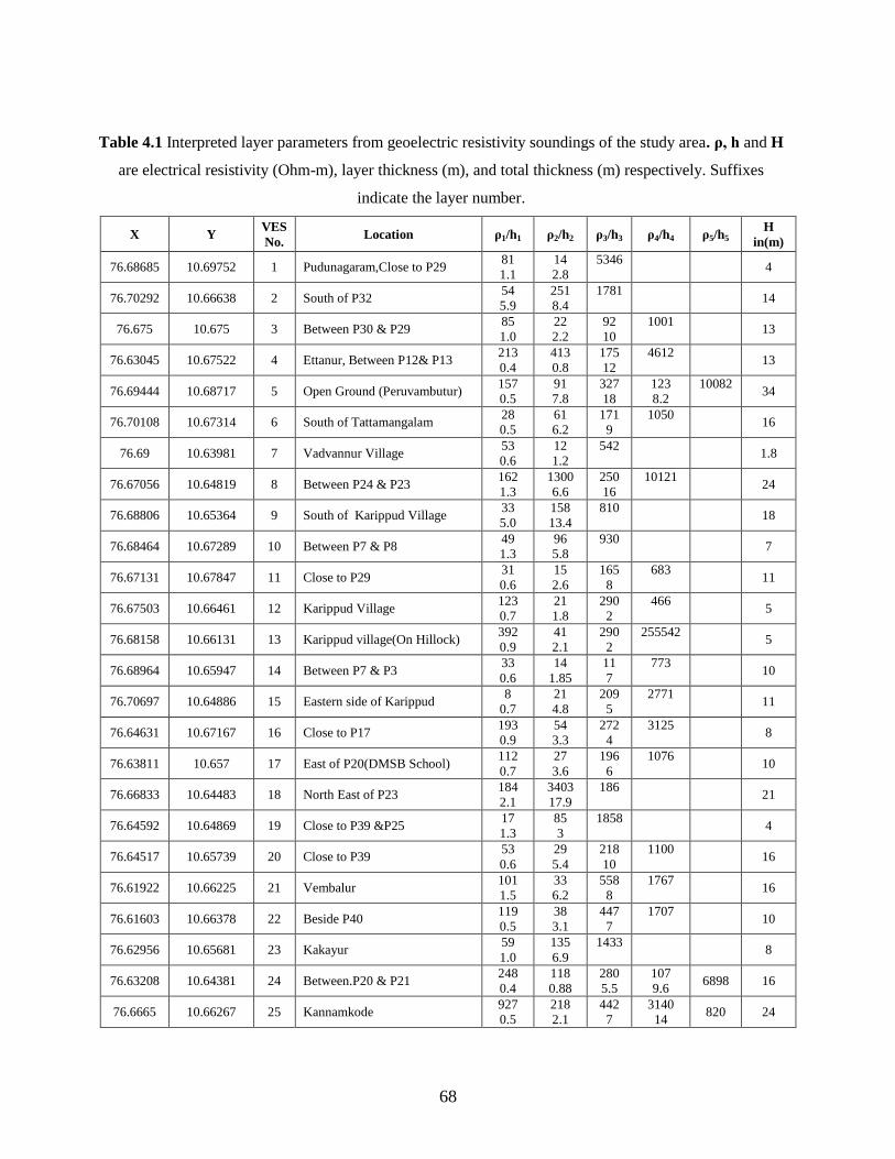
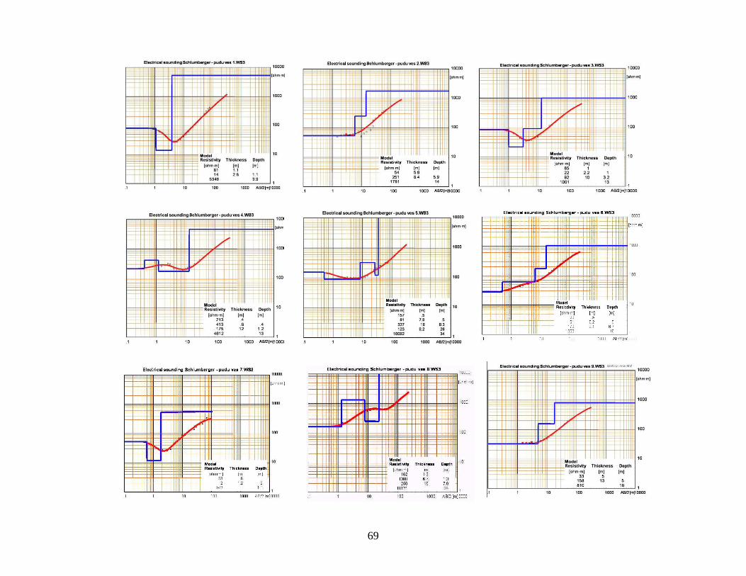
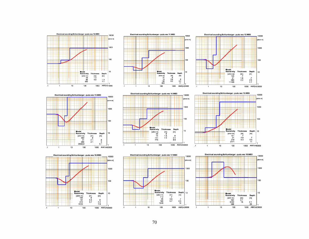
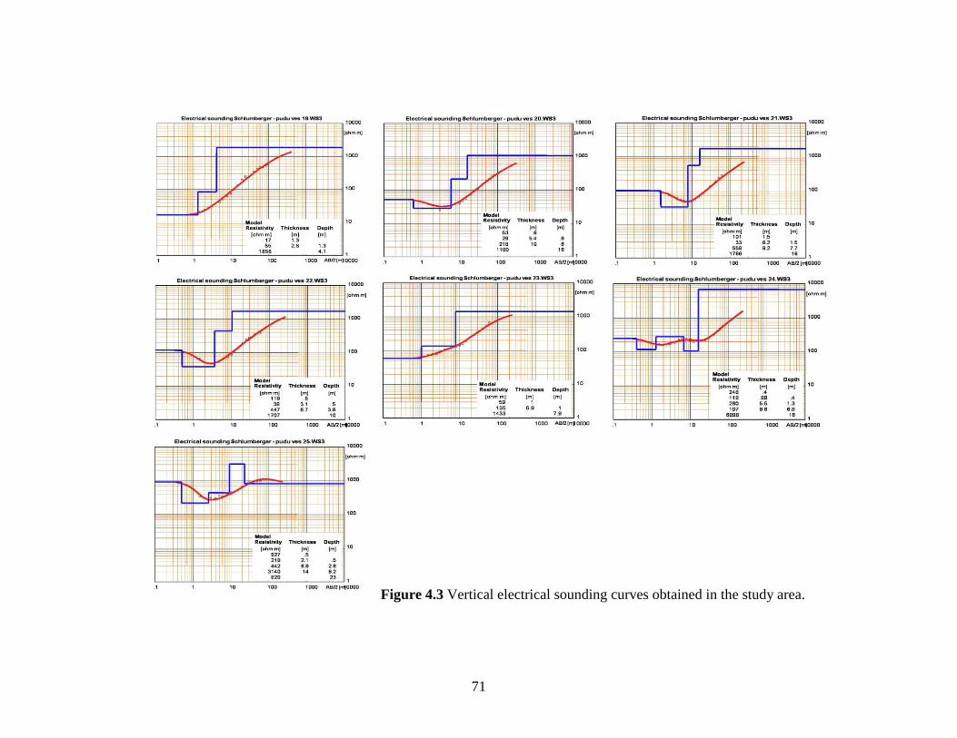
Table 4.1 gives the interpreted layer parameters (layer thickness and electrical
resistivity) of 25 VES. Typical sounding curves obtained in the study area, are shown in
Figure 4.3. The curves shows maximum of three layers. The maximum depth of
information of 34m is obtained at VES 5 and these values area well correlated with the
borehole lithologs drilled close to the observation wells. Majority of the sounding curves
are found as „H‟ type. Based on the VES locations VES Profile A-Al
is prepared covering
the VES locations from west to east in the study area.
68
Table 4.1 Interpreted layer parameters from geoelectric resistivity soundings of the study area. ρ, h and H
are electrical resistivity (Ohm-m), layer thickness (m), and total thickness (m) respectively. Suffixes
indicate the layer number.
X Y VES
No. Location ρ1/h1 ρ2/h2 ρ3/h3 ρ4/h4 ρ5/h5
H
in(m)
76.68685 10.69752 1 Pudunagaram,Close to P29 81
1.1
14
2.8
5346
4
76.70292 10.66638 2 South of P32 54
5.9
251
8.4
1781
14
76.675 10.675 3 Between P30 & P29 85
1.0
22
2.2
92
10
1001
13
76.63045 10.67522 4 Ettanur, Between P12& P13 213
0.4
413
0.8
175
12
4612
13
76.69444 10.68717 5 Open Ground (Peruvambutur) 157
0.5
91
7.8
327
18
123
8.2
10082
34
76.70108 10.67314 6 South of Tattamangalam 28
0.5
61
6.2
171
9
1050
16
76.69 10.63981 7 Vadvannur Village 53
0.6
12
1.2
542
1.8
76.67056 10.64819 8 Between P24 & P23 162
1.3
1300
6.6
250
16
10121
24
76.68806 10.65364 9 South of Karippud Village 33
5.0
158
13.4
810
18
76.68464 10.67289 10 Between P7 & P8 49
1.3
96
5.8
930
7
76.67131 10.67847 11 Close to P29 31
0.6
15
2.6
165
8
683
11
76.67503 10.66461 12 Karippud Village 123
0.7
21
1.8
290
2
466
5
76.68158 10.66131 13 Karippud village(On Hillock) 392
0.9
41
2.1
290
2
255542
5
76.68964 10.65947 14 Between P7 & P3 33
0.6
14
1.85
11
7
773
10
76.70697 10.64886 15 Eastern side of Karippud 8
0.7
21
4.8
209
5
2771
11
76.64631 10.67167 16 Close to P17 193
0.9
54
3.3
272
4
3125
8
76.63811 10.657 17 East of P20(DMSB School) 112
0.7
27
3.6
196
6
1076
10
76.66833 10.64483 18 North East of P23 184
2.1
3403
17.9
186
21
76.64592 10.64869 19 Close to P39 &P25 17
1.3
85
3
1858
4
76.64517 10.65739 20 Close to P39 53
0.6
29
5.4
218
10
1100
16
76.61922 10.66225 21 Vembalur 101
1.5
33
6.2
558
8
1767
16
76.61603 10.66378 22 Beside P40 119
0.5
38
3.1
447
7
1707
10
76.62956 10.65681 23 Kakayur 59
1.0
135
6.9
1433
8
76.63208 10.64381 24 Between.P20 & P21 248
0.4
118
0.88
280
5.5
107
9.6 6898 16
76.6665 10.66267 25 Kannamkode 927
0.5
218
2.1
442
7
3140
14 820 24
69
70
71
Figure 4.3 Vertical electrical sounding curves obtained in the study area.
72
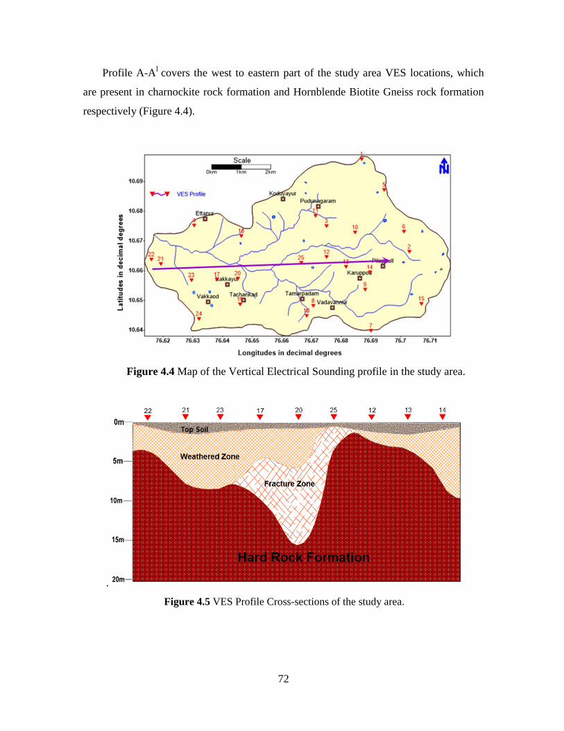
Profile A-Al covers the west to eastern part of the study area VES locations, which
are present in charnockite rock formation and Hornblende Biotite Gneiss rock formation
respectively (Figure 4.4).
Figure 4.4 Map of the Vertical Electrical Sounding profile in the study area.
.
Figure 4.5 VES Profile Cross-sections of the study area.
73
Based on the VES data interpretation it is found that the top soil zone present up to
2 m depth with the resistivity value 8-50 Ω-m and the depth to hard rock varies from 4 to
16m. The shallow hard rock was found in the upstream area at depth of 3m. The thickness
of weathering is more than 6m. In addition, weathered zone thickness is found to be
increased in the middle and downstream (west) of the study area with the resistivity value
20-100 Ω-m, which is bearing fresh groundwater with Total Dissolved Solids (TDS)
value from 100-1000 mg/l. Moreover, it is acting as a potential zone for the wells.
Fractured zone was encountered in middle portion of the study area at depth of 2 to 15m
with the resistivity 150-220 Ω-m (Figure 4.5). The bore wells up to 40m in this region are
found with 3-5 inch of yield.
4.8 Multi-electrode resistivity imaging (MERI)
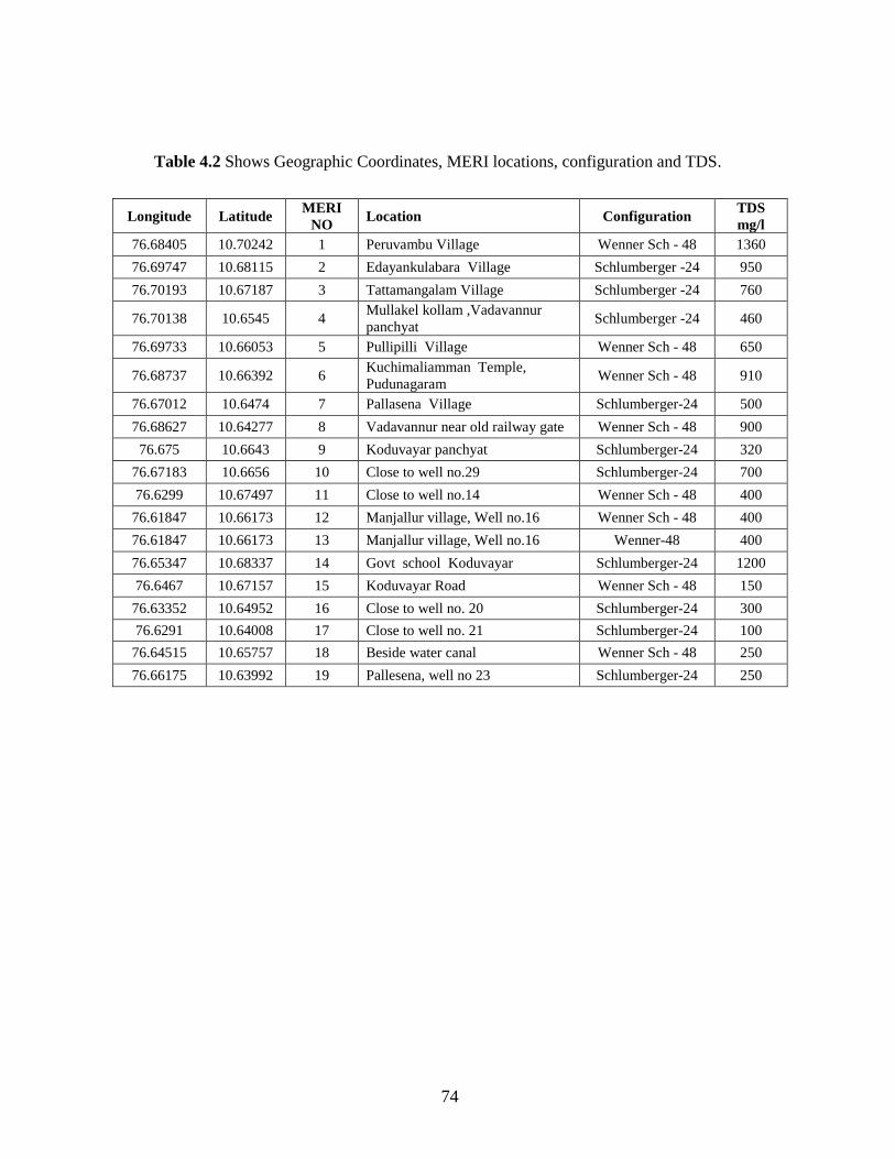
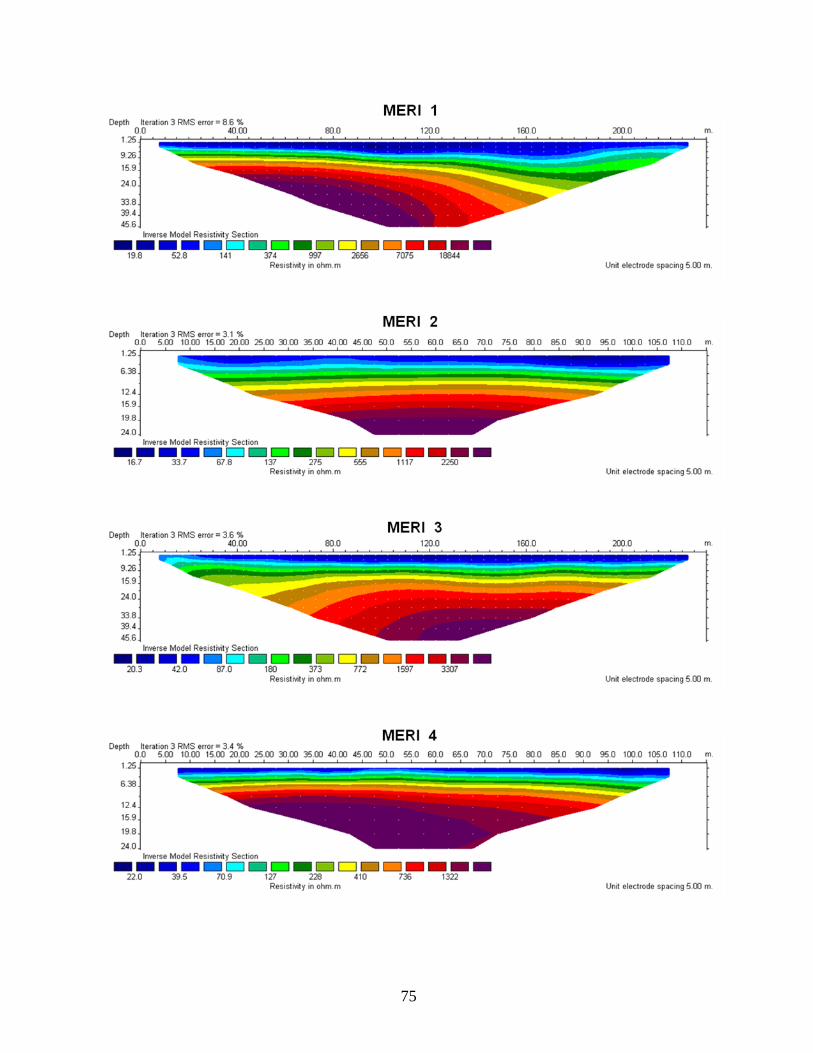
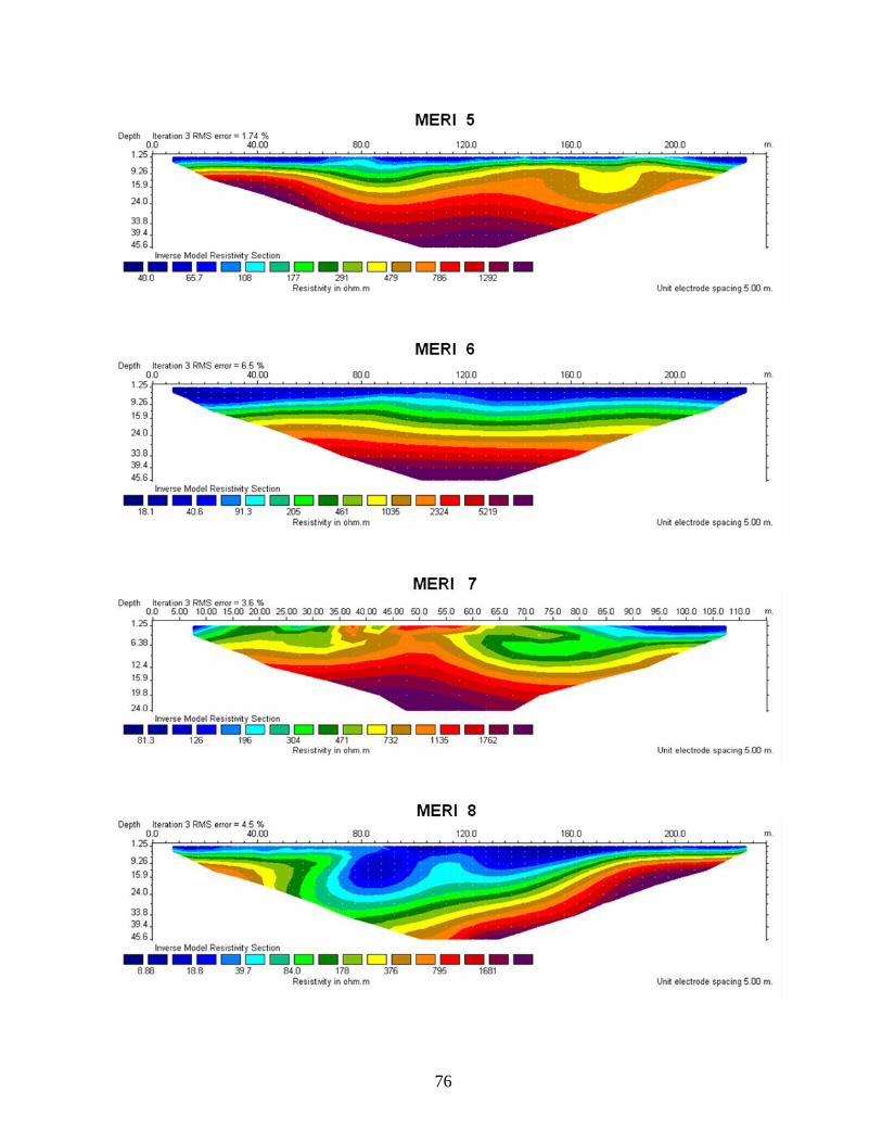
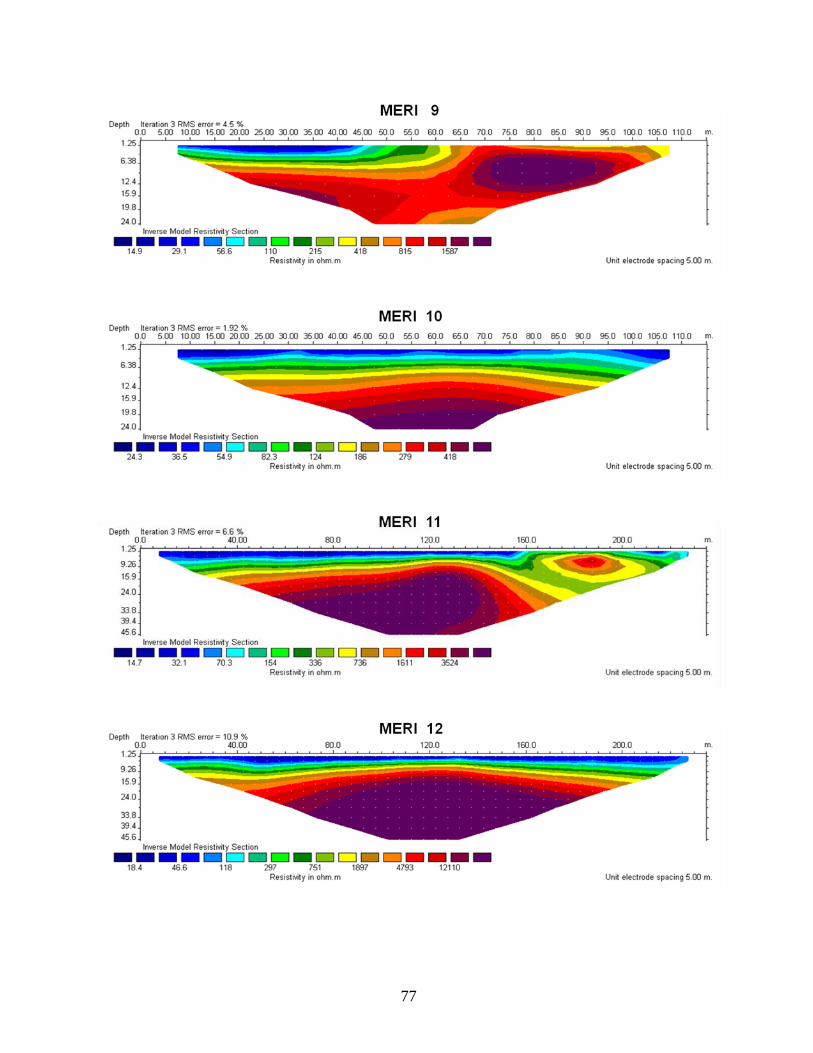
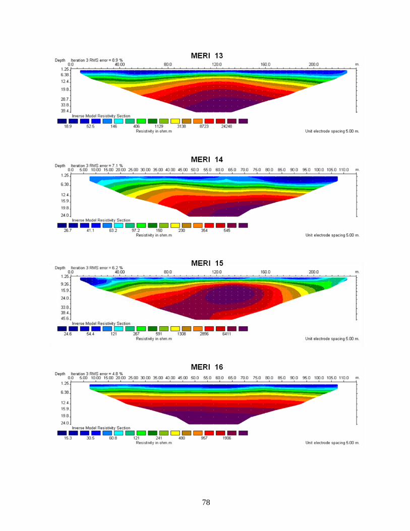
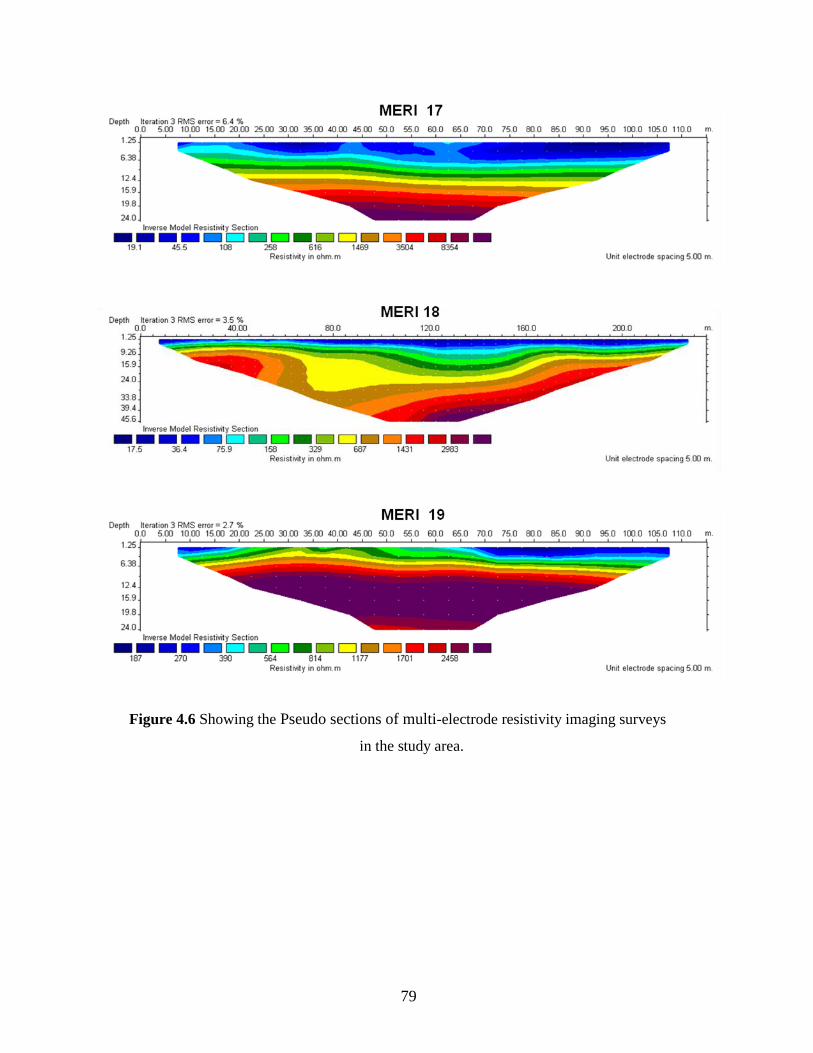
Table 4.2 presents the detail information of MERI surveys in the study area. The
details indicate location, geo-coordinates, configuration and number of electrodes used.
The software known as RES2DINV is used to prepare the „Inverse Model Resistivity
Sections‟ and the Iteration RMS error (route mean square) were observed to be below 10.
During process/interpretation of the raw data, an option called „Exterminate bad datum
points‟ was used to reduce the RMS error. The MERI images (Figure 4.6) shows 2D
images of inverse model resistivity sections with label indicating resistivity ranges in
various color. Due to the wide resistivity ranges, the color code of resistivity range is kept
specific to the images.
74
Table 4.2 Shows Geographic Coordinates, MERI locations, configuration and TDS.
Longitude Latitude MERI
NO Location Configuration
TDS
mg/l
76.68405 10.70242 1 Peruvambu Village Wenner Sch - 48 1360
76.69747 10.68115 2 Edayankulabara Village Schlumberger -24 950
76.70193 10.67187 3 Tattamangalam Village Schlumberger -24 760
76.70138 10.6545 4 Mullakel kollam ,Vadavannur
panchyat Schlumberger -24 460
76.69733 10.66053 5 Pullipilli Village Wenner Sch - 48 650
76.68737 10.66392 6 Kuchimaliamman Temple,
Pudunagaram Wenner Sch - 48 910
76.67012 10.6474 7 Pallasena Village Schlumberger-24 500
76.68627 10.64277 8 Vadavannur near old railway gate Wenner Sch - 48 900
76.675 10.6643 9 Koduvayar panchyat Schlumberger-24 320
76.67183 10.6656 10 Close to well no.29 Schlumberger-24 700
76.6299 10.67497 11 Close to well no.14 Wenner Sch - 48 400
76.61847 10.66173 12 Manjallur village, Well no.16 Wenner Sch - 48 400
76.61847 10.66173 13 Manjallur village, Well no.16 Wenner-48 400
76.65347 10.68337 14 Govt school Koduvayar Schlumberger-24 1200
76.6467 10.67157 15 Koduvayar Road Wenner Sch - 48 150
76.63352 10.64952 16 Close to well no. 20 Schlumberger-24 300
76.6291 10.64008 17 Close to well no. 21 Schlumberger-24 100
76.64515 10.65757 18 Beside water canal Wenner Sch - 48 250
76.66175 10.63992 19 Pallesena, well no 23 Schlumberger-24 250
75
76
77
78
79
Figure 4.6 Showing the Pseudo sections of multi-electrode resistivity imaging surveys
in the study area.
80
Possible drilling locations have been suggested based on resistivity data for the deeper
bore wells for lithology collection and slim holes for moisture measurement studies.
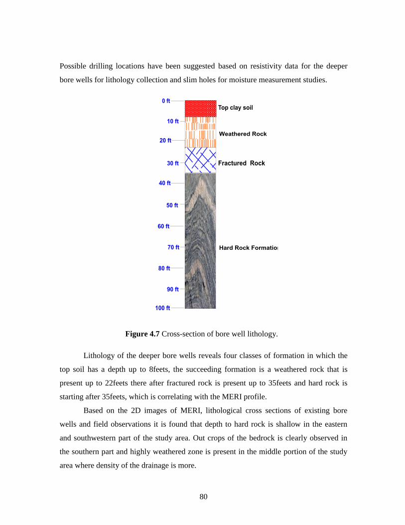
Figure 4.7 Cross-section of bore well lithology.
Lithology of the deeper bore wells reveals four classes of formation in which the
top soil has a depth up to 8feets, the succeeding formation is a weathered rock that is
present up to 22feets there after fractured rock is present up to 35feets and hard rock is
starting after 35feets, which is correlating with the MERI profile.
Based on the 2D images of MERI, lithological cross sections of existing bore
wells and field observations it is found that depth to hard rock is shallow in the eastern
and southwestern part of the study area. Out crops of the bedrock is clearly observed in
the southern part and highly weathered zone is present in the middle portion of the study
area where density of the drainage is more.
81
4.9 Summary
Based on geophysical investigations supported by hydrochemical data the
following important inferences were made in conceptualizing the aquifer system and to
demarcate groundwater potential zones and subsurface conditions.
Geophysical investigations VES, MERI and drilling lithologs, revealed the general
lithology of the study area.
The VES curves shows maximum of three layers and maximum depth of
information of 12m is obtained. Majority of the sounding curves are found as „H‟
type.
Based on the VES data interpretation it is found that the top soil zones present up
to 2 m depth with the resistivity value 8-50 Ω-m. Moreover, the depth to hard rock
varies from 4 to 16m.
The shallow hard rock was found in the upstream area at depth of 3m. Out crops
of the bedrock is clearly observed in the southern portion of the area. Fractured
zone was encountered in middle portion of the study area at depth of 2 to 15m
with the resistivity 150-220 Ω-m.
Weathered zone thickness is found to be increased in the middle and downstream
(west) of the study area with the resistivity value 20-100 Ω-m and thickness of
weathering is more than 6m where density of the drainage is more. In addition, it
is acting as a potential zone for the wells to bearing fresh groundwater.
Lithology of the deeper bore wells reveals four classes of formation in which the
top soil has a depth up to 8feets, the succeeding formation is a weathered rock that
is present up to 22feet there after fractured rock is present up to 35feet and hard
rock is encountered after 35feet, which is correlates with the MERI profile.
82
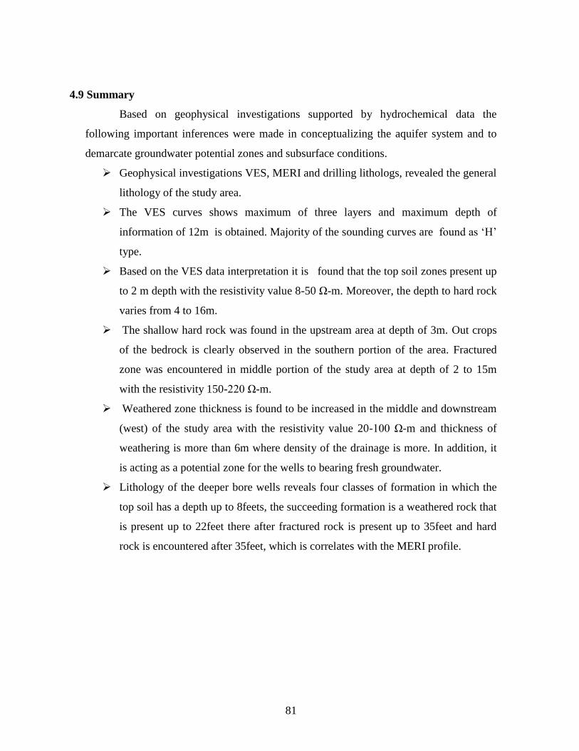
Plate 4.1 Vertical Electrical Sounding in the paddy field in the study area.
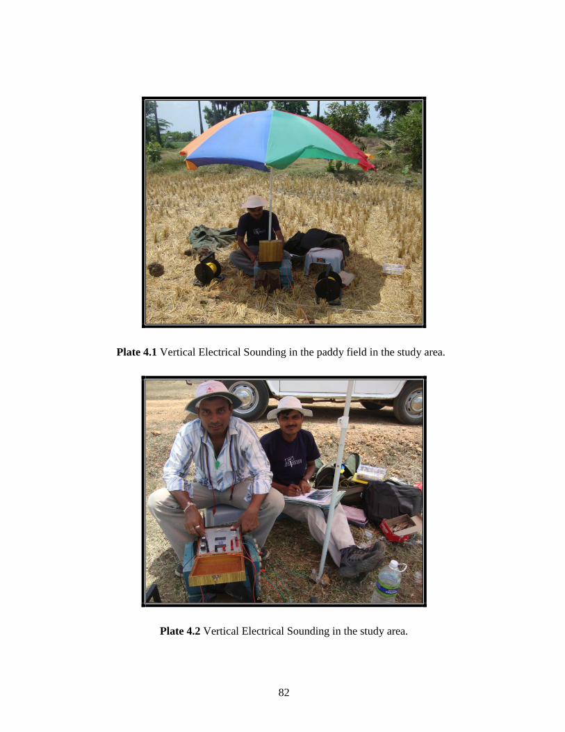
Plate 4.2 Vertical Electrical Sounding in the study area.
83
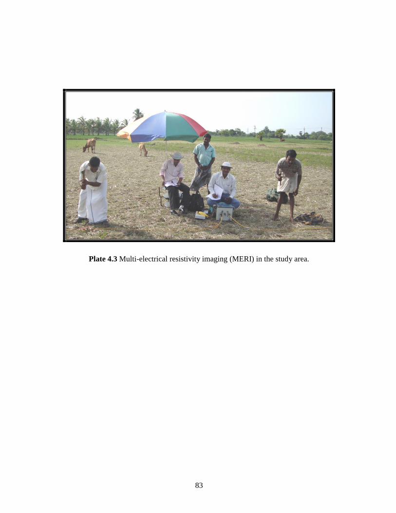
Plate 4.3 Multi-electrical resistivity imaging (MERI) in the study area.