chapter 4. interpolation interpolation - texas a&m …dallen/m609_05c/chapter4.pdf · 1 chapter...
TRANSCRIPT
1
Chapter 4. Interpolation
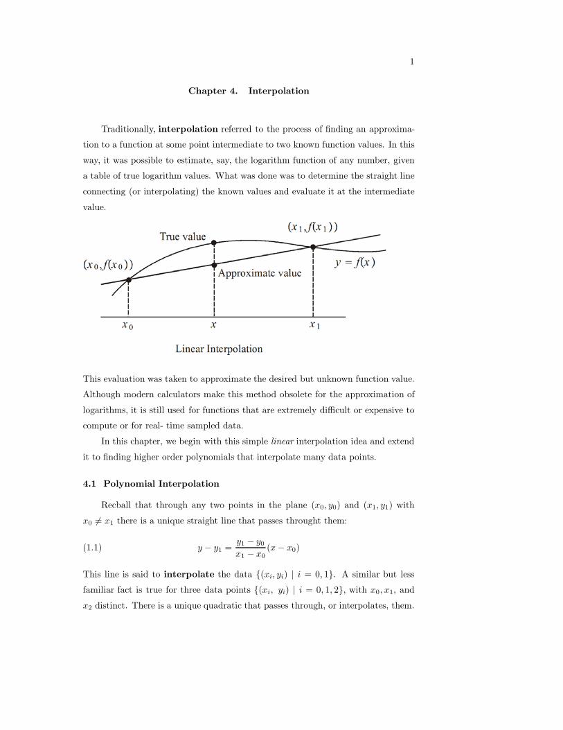
Traditionally, interpolation referred to the process of finding an approxima-
tion to a function at some point intermediate to two known function values. In this
way, it was possible to estimate, say, the logarithm function of any number, given
a table of true logarithm values. What was done was to determine the straight line
connecting (or interpolating) the known values and evaluate it at the intermediate
value.
This evaluation was taken to approximate the desired but unknown function value.
Although modern calculators make this method obsolete for the approximation of
logarithms, it is still used for functions that are extremely difficult or expensive to
compute or for real- time sampled data.
In this chapter, we begin with this simple linear interpolation idea and extend
it to finding higher order polynomials that interpolate many data points.
4.1 Polynomial Interpolation
Recball that through any two points in the plane (x0, y0) and (x1, y1) with
x0 �= x1 there is a unique straight line that passes throught them:
(1.1) y − y1 =y1 − y0
x1 − x0(x − x0)
This line is said to interpolate the data {(xi, yi) | i = 0, 1}. A similar but less
familiar fact is true for three data points {(xi, yi) | i = 0, 1, 2}, with x0, x1, and
x2 distinct. There is a unique quadratic that passes through, or interpolates, them.
4.1 Polynomial Interpolation 2
Finding this quadratic and higher order polymomials for more data points is the
subject of this chapter. To begin let us make our notions precise.
Given n+1 data points {(xi, yi) | i = 0, 1, . . . , n} with all xi, i = 0, 1, . . . , n
distinct. In many texts the values xi, i = 0, 1, . . . , n are called the nodes. A
function F (x) that satifies the conditions
(1.2) F (xi) = yi, i = 0, 1, . . . , n
is said to interpolate the data. The process of finding F (x) is called interpolation
and F (x) is called an interpolating function. If F (x) = p(x) is a polynomial then
p(x) is called an interpolating polynomial. For all of the sections of this chap-
ter, except the last, we will be concerned with the determination of interpolating
polynomials. In order that a unique solution exist to the problem of finding inter-
polating polynomials we add in the interpolation problem below the extra condition
that the polynomial be of smallest possible degree.
Interpolation Problem. Given n + 1 data points {(xi, yi) | i = 0, 1, . . . , n}with xi, i = 0, 1, . . . , n distinct. Find a polynomial of smallest possible degree
that interpolates the data; that is, satisfies (1.2).
Five relevant questions immediately arise.
1. Does such an interpolating polynomial exist? And if so,
2. How can it be determined?
3. What is its degree?
4. Is it unique?
5. Suppose the data are sampled. That is, suppose there is an underlying function
f(x) for which yi = f(xi), i = 0, 1, . . . , n. Can we estimate the error of
approximation
f(x) − p(x)
for values of x �= xi, i = 0, 1, . . . , n?
It is easy to see that an interpolating polynomial exists. To show this we proceed by
induction. First of all, in the case n = 0 (one data point), the 0th degree polynomial
4.1 Polynomial Interpolation 3
y = y0 interpolates (x0, y0). For two data points {(xi, yi), i = 0, 1}, the polynomial
of 1st degree (a linear function) was constructed in (1.1) above. Now suppose
that a polynomial pn−1(x) of degree n − 1 interpolates the data {(xi, yi), i =
0, 1, . . . , n− 1}. Define
(1.3) pn(x) = pn−1(x) + cn(x − x0)(x − x1) · · · (x − xn−1)
Then pn(x) also interpolates the data {(xi, yi), i = 0, 1, . . . , n − 1}. Since all the
xi, i = 0, 1, . . . , n are distinct we can solve the equation
pn(xn) = pn−1(xn) + cn(xn − x0)(xn − x1) · · · (xn − xn−1) = yn
for c. Thus
(1.4) cn =yn − pn−1(xn)
(xn − x0)(xn − x1) · · · (xn − xn−1)
Constructed in this way the interpolating polynomial has the form
(1.5)
pn(x) = c0 + c1(x−x0)+ c2(x−x0)(x−x1)+ · · ·+ cn(x−x0)(x−x1) · · · (x−xn−1)
with the coefficients c0, c1, . . . , cn computed inductively. Importantly, it has degree
at most n. In fact, the degree of pn(x) can be strictly less that n. For example,
observe that the three data points (0,1), (1,2), and (2,3) are interpolated by the
polynomial of degree 1, y = x + 1. (For correct mathematical interpretation, how-
ever, this linear polynomial is also to be considered quadratic.) As we show in the
following example, formulas (1.3) and (1.4) can be used to construct the interpolat-
ing polynomial. But more efficient methods, such as Newton’s Forward Difference
Method, are derived in the next section.
Example 1.1. Use formulas (1.3) and (1.4) to interpolate the data (1,3), (2,5),
and (3,1).
Solution. First we use formula (1.1) to write a formula for the degree 1 that
interpolates (1,3) and (2,5). It is
y − 3 =5 − 32 − 1
(x − 1)
= 2x− 2
y = 2x + 1 (= p1(x)
4.1 Polynomial Interpolation 4
From (1.3) we see that p2(x) has the form
p2(x) = p1(x) + c2(x − 1)(x − 2)
= 2x + 1 + c(x − 1)(x − 2)
Substitute x = 3 into p2(x) above and solve
p2(3) = 2(3) + 1 + c2(3 − 1)(3 − 2) = 1
c2 =−6
(2)(1)= −3
So,p2(x) = 2x + 1 − 3(x − 1)(x − 2)
= 2x + 1 − 3(x2 − 3x + 2)
= −3x2 + 11x − 5
Notice that the degree is 2, one less that the number of data points. There are
many interpolating polynomials that interpolate a given set of data. For example,
the cubic polynomial
p(x) = −3x2 + 11x − 5 + a(x − 1)(x − 2)(x − 3)
interpolates the data of Example 1 for every value of a. But what is true is that there
exists a unique polynomial of degree n that interpolates {(xi, yi), i = 0, 1, . . . , n}.To show this we require the following fact: Every non zero polynomial of degree n
has at most n zeros*. So, if p(x) and q(x) are two polynomials, each of at most
degree n that interpolate the data {(xi, yi), i = 0, 1, . . . , n}, then the difference
r(x) = p(x) − q(x)
is also a polynomial of at most degree n for which r(xi) = 0, i = 0, 1, . . . , n. That
is, r(x) has n + 1 zeros. This cannot happen unless r(x) = 0 for all x. And this
means, of course, that r(x) is the zero polynomial. Let us summarize the discussion
above in the following
Theorem. Given the n + 1 data points {(xi, yi), i = 0, 1, . . . , n}, with
xi, i = 0, 1, . . . , n distinct. Then there exists a unique polynomial p(x) of degree
n that interpolates the data.
* If the nth degree polynomial has a nonzero coefficient multiplying xn, then it
has exactly n zeros. See, Section (2.3).
4.1 Polynomial Interpolation 5
This theorem implies that if the same data {(xi, yi), i = 0, 1, . . . , n} is
interpolated by two polynomials, both of at most degree n, then they must be the
same, even though they may have different forms.
Thus, we have answered the first four of the basic questions above. There is a
polynomial of degree at most n that interpolates the data {(xi, yi), i = 0, 1, . . . , n},and formulas (1.3) and (1.4) can be used to find it. The fifth question will be
answered in Section 4.3.
4.1 Polynomial Interpolation 6
Exercises 4.1
In Problems 1-6 evaluate the given polynomial at the given x-coordinates.
1. p(x) = 1 + 3(x − 2) x = 2, 4
2. p(x) = 3 + 12(x− 23), x = 23, 43
3. p(x) = 4 + 2(x − 5) − 3(x − 5)(x + 1), x = 5, −1, 2
4. p(x) = −3.1 + 3.5(x− 1.3) + 2.0(x− 1.3)(x− 2.7), x = 1.3, 3.7, 8.1
5. p(x) = 2.1+6.0(x+2.1)+0.5(x+2.1)(x+1.7)−1.7(x+2.1)(x+1.7)(x−3.3),
x = −2.1,−1.7, 3.3, 8.9
6. p(x) = 1.9(x− 4.1) + 2.0(x− 4.1)(x + 2.2) + 1.8x(x− 4.1)(x + 2.2),
x = 4.1,−2.2, 01.8
In Problems 6-14 use formulas (1.3) and (1.4) to find the interpolating polynomial
for the given data.
7. (0,1), (1,2), (2,5)
8. (2,-5), (-1,-8), (0,-11)
9. (-1,4), (0,3), (1,8), (2,31)
10. (1.30, -2.0), ( -1.20, 2.5), ( 3.40, 23.2), ( 4.90, 192.454)
11. (6.1, 5.6), (4.7, 5.9), (2.9, 29.0), (-1.2, 183)
12. ( .10, 4.0), ( .24, 4.42), ( 5.60, 79.46), ( 7.10, 193.07)
13. ( -2 , 1 ), ( -1 , 3 ), ( 0 , 7 ), ( 1 , 25 ), ( 2 , 93 )
14. ( -4 , -2 ), ( -1 , -5 ), ( 3 , 190), ( 5, 367 ), ( 6 , 898 )
In Problems 15-20 find the interpolating polynomial for the data {(xi, f(xi), i =
0, 1, . . . , n} where f(x) and {xi, i = 0, 1, . . . , n} are given.
15. f(x) = ex, x = −1, 0, 1.
16. f(x) = sin x, x = π/6, π/4, π/2.
17. f(x) =1
x2 + 1, x = 1, 2, 3.
18. f(x) =1
x + 2, x = −1, 0, 1.
7
19. f(x) =x2 + 1x + 1
, x = −.5, 0, .5, 1.
20. f(x) = 3x3 − 2x2 + x − 5, x = −1, 0, 1 , 2.
21. Find the quadratic polynomial p2(x) that interpolates the function f(x) =
3x2 + 2x − 2 at x = 0, 1, and 2. Now simplify p2(x). What do you observe?
22. The most common form of a polynomial of nth degree is
qn(x) = a0 + a1x + a2x2 + · · ·+ anxn.
Determine an (n + 1) × (n + 1) linear system of equations in the variables
a0, a1, . . . , an whose solution make qn(x) a solution of the interpolation problem
for the data
{(xi, yi), i = 0, 1, . . . , n}.
Computer Exercises
I. Write a computer program that uses formulas (1.3) and (1.4) to determine the
interpolating polynomial of a given set of data. Input the value n, and the
data. Check to see if the x−coordinates are distinct. Output the coefficients
c0, c1, . . . , cn.
Applications. Use program I to interpolate the data sets given below.
Data sets to be inserted
II. From formula (1.5) we can define an (n + 1) × (n + 1) lower triangular linear
system of equations for the coefficients c0, c1, . . . , cn.
c0 = y0
c0 + c1(x1 − x0) = y1
c0 + c1(x2 − x0) + c2(x2 − x0)(x2 − x1) = y2
...
c0 + c1(xn − x0) + c2(xn − x0)(xn − x1) + · · ·+ cn(xn − x0) · · · (xn − xn−1) = yn
This system can be solved by back substitution. Write a program to find
c0, c1, . . . , cn from this system using back substitution.
4.2 Lagrange and Newton Methods
4.2 Lagrange and Newton Methods 8
Two methods, the Lagrange and the Newton methods, are presented in this sec-
tion. Basically, they are different in scope. The Lagrange Method, while rarely used
in practice, is very useful for proving various facts about interpolating polynomials.
The Newton Method is in general use today, because it is simple to implement,
simple to update with new data, and is computationally, the most efficient.
The Lagrange Method
Consider just three data points (x0, y0), (x1, y1), and (x2, y2). We know from
the previous section that there is a quadratic that interpolates this data. Define
the three basis functions
(2.1)
�2,0(x) =(x − x1)(x − x2)
(x0 − x1)(x0 − x2)
�2,1(x) =(x − x0)(x − x2)
(x1 − x0)(x1 − x2)
�2,2(x) =(x − x0)(x − x1)
(x2 − x0)(x2 − x1)
Observe that �2,0(x) interpolates the data (x0, 1), (x1, 0), and (x2, 0). Then y0�2,0(x)
interpolates the data (x0, y0), (x1, 0), and (x2, 0). Similarly y1�2,1(x) interpo-
lates the data (x0, 0), (x1, y1), and (x2, 0), and y2�2,2(x) interpolates the data
(x0, 0), (x1, 0), and (x2, y2). Now define
(2.2) p2(x) = y0�2,0(x) + y1�2,1(x) + y2�2,2(x).
By summing we see that p2(x), which has degree at most two, interpolates the
given data (xi, yi), i = 0, 1, 2. Written as above, p2(x) is called the Lagrange
interpolating polynomial of the three given data points.
Example 2.1. Determine the Lagrange interpolating polynomial of the data
(1,3), (2,5), and (3,1).
Solution. We have
�2,0(x) =(x − 2)(x − 3)(1 − 2)(1 − 3)
=12(x − 2)(x − 3)
�2,1(x) =(x − 1)(x − 3)(2 − 1)(2 − 3)
= −(x − 1)(x − 3)
�2,2(x) =(x − 1)(x − 2)(3 − 1)(3 − 2)
=12(x − 1)(x − 2)
4.2 Lagrange and Newton Methods 9
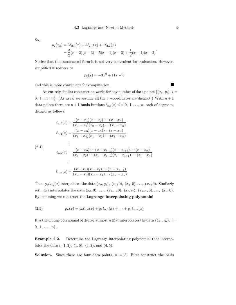
So,p2(xx) = 3�2,0(x) + 5�2,1(x) + 1�2,2(x)
=32(x − 2)(x − 3) − 5(x − 1)(x − 3) +
12(x − 1)(x − 2)
.
Notice that the constructed form it is not very convenient for evaluation. However,
simplified it reduces to
p2(x) = −3x2 + 11x − 5
and this is more convenient for computation.
An entirely similar construction works for any number of data points {(xi, yi), i =
0, 1, . . . , n}. (As usual we assume all the x -coordinates are distinct.) With n + 1
data points there are n +1 basis funtions �n,i(x), i = 0, 1, . . . , n, each of degree n,
defined as follows:
(2.4)
�n,0(x) =(x − x1)(x − x2) · · · (x − xn)
(x0 − x1)(x0 − x2) · · · (x0 − xn)
�n,1(x) =(x − x0)(x − x2) · · · (x − xn)
(x1 − x0)(x1 − x2) · · · (x1 − xn)...
�n,i(x) =(x − x0) · · · (x − xi−1)(x − xi+1) · · · (x − xn)
(xi − x0) · · · (xi − xi−1)(xi − xi+1) · · · (xi − xn)...
�n,n(x) =(x − x0)(x − x1) · · · (x − xn−1)(xn − x0)(xn − x1) · · · (xn − xn)
Then y0�n,0(x) interpolates the data (x0, y0), (x1, 0), (x2, 0), . . . , (xn, 0). Similarly
yi�n,i(x) interpolates the data (x0, 0), . . . , (xi−1, 0), (xi, yi), (xi+1, 0), . . . , (xn, 0).
By summing we construct the Lagrange interpolating polynomial
(2.5) pn(x) = y0�n,0(x) + y1�n,1(x) + · · ·+ yn�n,n(x)
It is the unique polynomial of degree at most n that interpolates the data {(xi, yi), i =
0, 1, . . . , n}.
Example 2.2. Determine the Lagrange interpolating polynomial that interpo-
lates the data (−1, 2), (1, 0), (3, 2), and (4, 5).
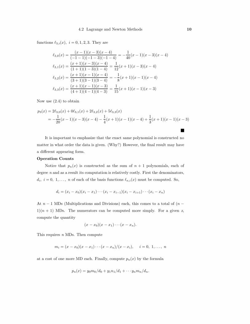
Solution. Since there are four data points, n = 3. First construct the basis
4.2 Lagrange and Newton Methods 10
functions �3,i(x), i = 0, 1, 2, 3. They are
�3,0(x) =(x − 1)(x − 3)(x − 4)
(−1 − 1)(−1 − 3)(−1 − 4)= − 1
40(x − 1)(x − 3)(x − 4)
�3,1(x) =(x + 1)(x − 3)(x − 4)(1 + 1)(1 − 3)(1 − 4)
=112
(x + 1)(x − 3)(x − 4)
�3,2(x) =(x + 1)(x − 1)(x − 4)(3 + 1)(3 − 1)(3 − 4)
= −18(x + 1)(x − 1)(x − 4)
�3,3(x) =(x + 1)(x − 1)(x − 3)(4 + 1)(4 − 1)(4 − 3)
=115
(x + 1)(x − 1)(x − 3)
Now use (2.4) to obtain
p3(x) = 2�3,0(x) + 0�3,1(x) + 2�3,2(x) + 5�3,3(x)
= − 120
(x − 1)(x − 3)(x − 4) − 14(x + 1)(x − 1)(x − 4) +
13(x + 1)(x − 1)(x − 3)
It is important to emphasize that the exact same polynomial is constructed no
matter in what order the data is given. (Why?) However, the final result may have
a different appearing form.
Operation Counts
Notice that pn(x) is constructed as the sum of n + 1 polynomials, each of
degree n and as a result its computation is relatively costly. First the denominators,
di, i = 0, 1, . . . , n of each of the basis functions �n,i(x) must be computed. So,
di = (xi − x0)(xi − x1) · · · (xi − xi−1)(xi − xi+1) · · · (xi − xn)
At n − 1 MDs (Multiplications and Divisions) each, this comes to a total of (n −1)(n + 1) MDs. The numerators can be computed more simply. For a given x,
compute the quantity
(x − x0)(x − x1) · · · (x − xn).
This requires n MDs. Then compute
mi = (x − x0)(x − x1) · · · (x − xn)/(x − xi), i = 0, 1, . . . , n
at a cost of one more MD each. Finally, compute pn(x) by the formula
pn(x) = y0m0/d0 + y1n1/d1 + · · ·ynmn/dn.
4.2 Lagrange and Newton Methods 11
This takes 2n+2 MDs. The total MDs is thus (n−1)(n+1)+n+(n+1)+(2n+2) =
n2 + 4n + 2 MDs. Note, however, that once the denominators di, i = 0, 1, . . . , n
and the factors yi/di, i = 0, 1, . . . , n have be calculated and stored, the net number
of MDs for each evaluation of pn(x) is only 3n+2 MDs. As we shall see, this is still
relatively costly.
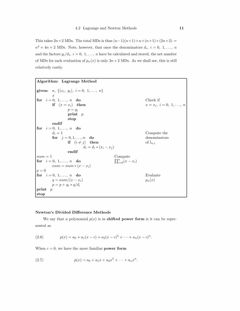
Algorithm: Lagrange Method
given: n, {(xi, yi), i = 0, 1, . . . , n}x
for i = 0, 1, . . . , n do Check ifif (x = xi) then x = xi, i = 0, 1, . . . , n
p = yi
print pstop
endiffor i = 0, 1, . . . , n do
di = 1 Compute thefor j = 0, 1, . . . , n do denominators
if (i �= j) then of ln,i
di = di ∗ (xi − xj)endif
num = 1 Computefor i = 0, 1, . . . , n do
∏ni=0(x − xi)
num = num ∗ (x − xi)p = 0for i = 0, 1, . . . , n do Evaluate
q = num/(x − xi) pn(x)p = p + yi ∗ q/di
print pstop
Newton’s Divided Difference Methods
We say that a polynomial p(x) is in shifted power form is it can be repre-
sented as
(2.6) p(x) = a0 + a1(x − c) + a2(x − c)2 + · · ·+ an(x − c)n.
When c = 0, we have the more familiar power form
(2.7) p(x) = a0 + a1x + a2x2 + · · ·+ anxn.
4.2 Lagrange and Newton Methods 12
Both forms occur in practice, especially when applying Taylor’s Theorem (see Sec-
tion 1.3). Another form, especially useful for constructing interpolating polyno-
mials, has already been encountered in Section 4.1. Called Newton’s form, it
requires n + 1 points xi, i = 0, 1, . . . , n, and has the form
(2.8)
p(x) = a0 +a1(x−x0)+a2(x−x0)(x−x1)+ · · ·+an(x−x0)(x−x1) · · · (x−xn−1).
If all the values xi, i = 0, 1, . . . , n are equal to c, then Newton’s form and the
shifted power form are the same. One important fact about all these forms is that
they can be computed using nested multiplication, which for (2.6), has the form
(2.9)
p(x) = [· · · [[an(x−xn−1)+an−1 ](x−xn−2)+an−2](x−xn−3)+· · ·+a1(x−x0)]+a0.
For example, the cubic 2x3 + 5x2 − 4x + 7 has the nested form
((2x + 5)x − 4)x + 7.
It is easy to see that the total number of MDs required for one evaluation of p(x)
is n.
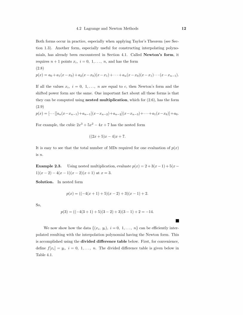
Example 2.3. Using nested multiplication, evaluate p(x) = 2 +3(x− 1)+5(x−1)(x − 2) − 4(x − 1)(x − 2)(x + 1) at x = 3.
Solution. In nested form
p(x) = ((−4(x + 1) + 5)(x − 2) + 3)(x − 1) + 2.
So,
p(3) = ((−4(3 + 1) + 5)(3 − 2) + 3)(3 − 1) + 2 = −14.
We now show how the data {(xi, yi), i = 0, 1, . . . , n} can be efficiently inter-
polated resulting with the interpolation polynomial having the Newton form. This
is accomplished using the divided difference table below. First, for convenience,
define f [xi] = yi, i = 0, 1, . . . , n. The divided difference table is given below in
Table 4.1.
4.2 Lagrange and Newton Methods 13
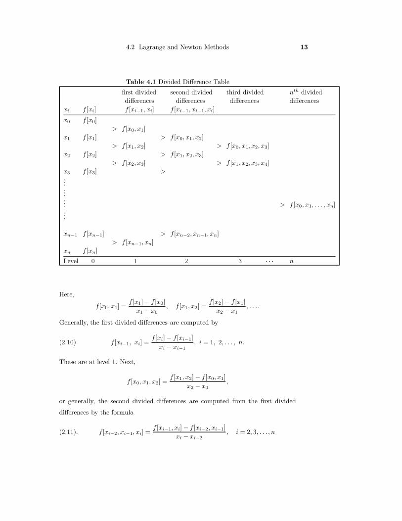
Table 4.1 Divided Difference Table
first divided second divided third divided nth divideddifferences differences differences differences
xi f [xi] f [xi−1, xi] f [xi−1, xi−1, xi]
x0 f [x0]> f [x0, x1]
x1 f [x1] > f [x0, x1, x2]> f [x1, x2] > f [x0, x1, x2, x3]
x2 f [x2] > f [x1, x2, x3]> f [x2, x3] > f [x1, x2, x3, x4]
x3 f [x3] >......... > f [x0, x1, . . . , xn]...
xn−1 f [xn−1] > f [xn−2, xn−1, xn]> f [xn−1, xn]
xn f [xn]
Level 0 1 2 3 · · · n
Here,
f [x0, x1] =f [x1] − f [x0]
x1 − x0, f [x1, x2] =
f [x2] − f [x1]x2 − x1
, . . . .
Generally, the first divided differences are computed by
(2.10) f [xi−1, xi] =f [xi] − f [xi−1]
xi − xi−1, i = 1, 2, . . . , n.
These are at level 1. Next,
f [x0, x1, x2] =f [x1, x2] − f [x0, x1]
x2 − x0,
or generally, the second divided differences are computed from the first divided
differences by the formula
(2.11). f [xi−2, xi−1, xi] =f [xi−1, xi] − f [xi−2, xi−1]
xi − xi−2, i = 2, 3, . . . , n
4.2 Lagrange and Newton Methods 14
These are at level 2. Successive divided differences are computed similarly; the level
k divided differences are computed from the formula
(2.12).
f [xi−k, xi−k+1, . . . , xi] =f [xi−k+1, . . . , xi] − f [xi−k, . . . , xi−1]
xi − xi−k, i = k, k+1 . . . , n
At each successive level there is one less divided difference than at the previous
level. At the nth, and last level, there is the single divided difference given by
f [x0, x1, . . . , xn] =f [x1, x2, . . . , xn] − f [x0, x2, . . . , xn−1]
xn − x0.myeqno
Note also that f [xi−k, xi−k+1, . . . , xi] depends only on the data points (xi−k, yi−k), . . . , (xi, yi).
There are several ways to use the divided difference table (Table 4.1) to de-
termine the interpolating polynomial. For example, by using the upper diagonal
of the table, we obtain the coefficients of the Newton forward difference formula as
follows. In (2.6) take
(2.13)
⎧⎪⎪⎪⎪⎪⎪⎪⎪⎨⎪⎪⎪⎪⎪⎪⎪⎪⎩
a0 = f [x0]a1 = f [x0, x1]...ai = f [x0, x1, . . . , xi]...an = f [x0, x1, . . . , xn]
Precisely, we have
Newton forward difference formula
Given the data {(xi, yi), i = 0, 1, . . . , n}, the Newton forward difference formula
is given by
(2.14)pn(x) = f [x0] + f [x0, x1](x− x0) + f [x0, x1, x2](x − x0)(x − x1)
+ · · ·+ f [x0, x1, . . . , xn](x− x0)(x − x1) · · · (x − xn−1)
where the coefficients f [x0, x1, . . . , xi], i = 0, 1, . . . , n are represented in Table
4.1 and computed from formula (2.11).
Specifically, (2.13) is called the Newton forward difference formula. Remember that,
although the Newton forward difference formula and the Lagrange interpolating
4.2 Lagrange and Newton Methods 15
polynomials for the same data may look different, they are exactly the same! This
is a consequence of the uniqueness result from Section 4.1, or alternatively, expand
them out to power form and note that the coefficients are the same.
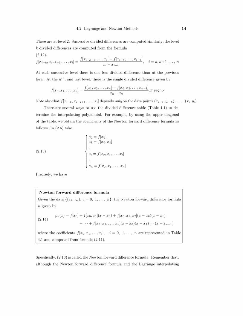
Example 2.4. Find the Newton forward difference formula for the data given in
Example 4.1.
Solution. Form the divided difference table
xi f [xi] f [xi−1, xi] f [xi−1, xi−1, xi]1 3
>5 − 32 − 1
= 2
2 5 >−4 − 23 − 1
= −3
>1 − 53 − 2
= −43 1
The coefficients 3, 2, and −3 are taken from the upper diagonal of the table. So
p2(x) = f [x0] + f [x0, x1](x − x0) + f [x0, x1, x2](x− x0)(x − x1)
= 3 + 2(x − 1) − 3(x − 1)(x − 2).
Simplification yields p2(x) = −3x2 + 11x− 5.
The term forward in the name of the Newton forward difference formula serves
to distinguish it from another, equivalent, interpolation polynomial. Called the
Newton backward difference formula it is given by
Newton backward difference formula
Given the data {(xi, yi), i = 0, 1, . . . , n}, the Newton backward difference formula
is given by
(2.15)pn(x) = f [xn] + f [xn−1, xn](x − xn) + f [xn−2, xn−1, xn](x− xn)(x − xn−1)
+ · · ·+ f [x0, x1, . . . , xn](x− xn)(x − xn−1) · · · (x − x1)
where the coefficients f [xi, xi+1, . . . , xn], i = 0, 1, . . . , n are represented in Table
4.1 and computed by (2.11).
Specifically, (2.14) is called the Newton backward difference formula. The coeffi-
cients are taken from the lower diagonal of the finite difference table. Therefore,
4.2 Lagrange and Newton Methods 16
it should be clear that the Newton backward difference formula is the same as the
Newton forward difference formula if the data were arranged in reverse order. For
the data of the previous example, the Newton backward difference formula has
coefficients 1, −4, and −3, yielding
p2(x) = 1 − 4(x − 3) − 3(x − 3)(x − 2)
Note that both the Newton forward and backward difference formulas are de-
noted by the same symbol, pn(x). Why?
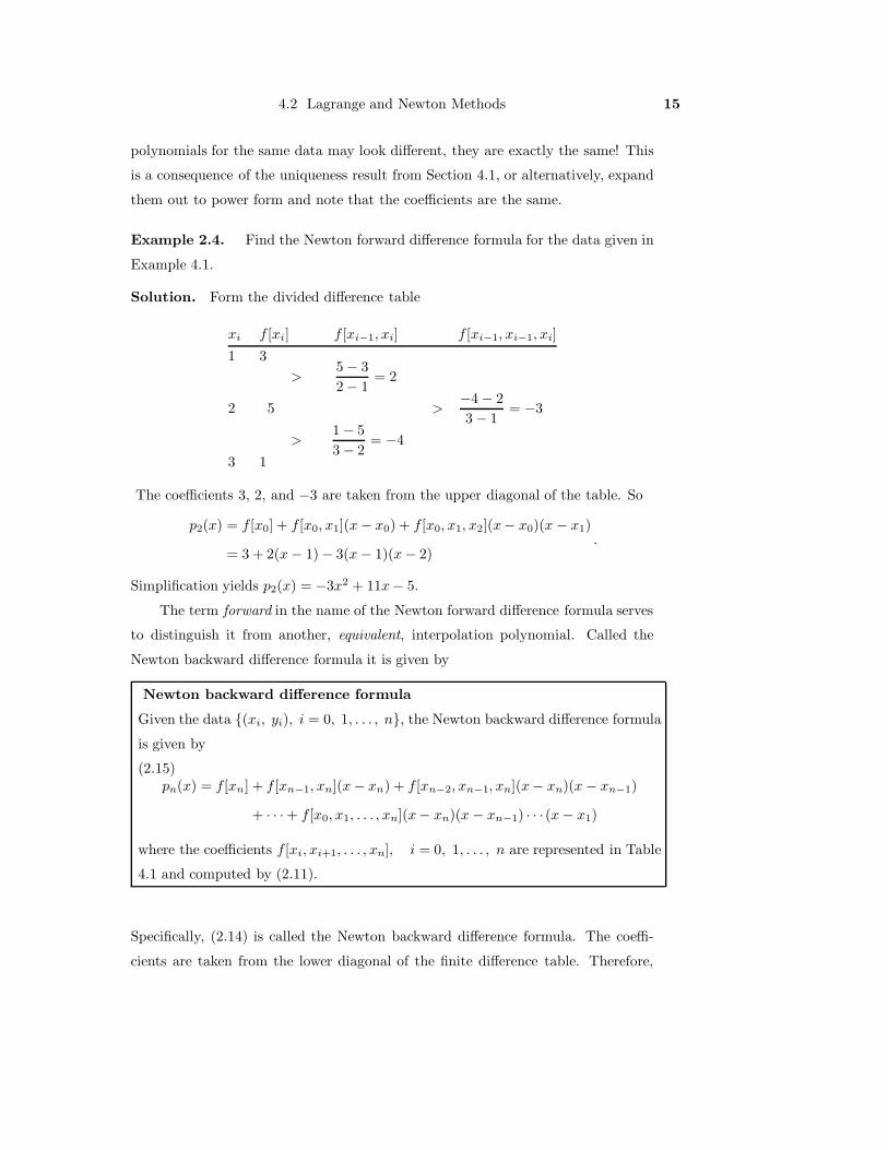
Example 2.5. Determine the Newton forward and backward difference polyno-
mials for the data in Example 4.2.
Solution. Form the divided difference table
xi f [xi] f [xi−1, xi] f [xi−1, xi−1, xi] f [x0, x1, x2, x3]
-1 2>
0 − 21 − (−1)
= −1
1 0 >1 − (−1)3 − (−1)
=12
>2 − 03 − 1
= 1 >23 − 1
2
4 − (−1)=
130
3 2 >3 − 14 − 1
=23
>5 − 24 − 3
= 34 5
The Newton forward difference formula is
p3(x) = 2 − (x + 1) +12(x + 1)(x − 1) +
130
(x + 1)(x − 1)(x − 3)
and the Newton backward difference formula is
p3(x) = 5 + 3(x − 4) +23(x − 4)(x − 3) +
130
(x − 4)(x − 3)(x − 1)
In the next example we consider data of the form (xi, f(xi)), i = 0, 1, . . . , n
where f(x) is some given function.
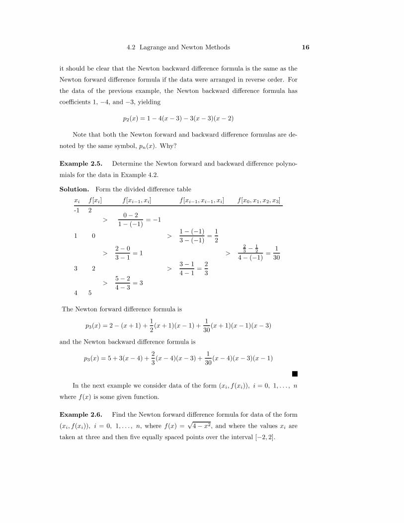
Example 2.6. Find the Newton forward difference formula for data of the form
(xi, f(xi)), i = 0, 1, . . . , n, where f(x) =√
4 − x2, and where the values xi are
taken at three and then five equally spaced points over the interval [−2, 2].
4.2 Lagrange and Newton Methods 17
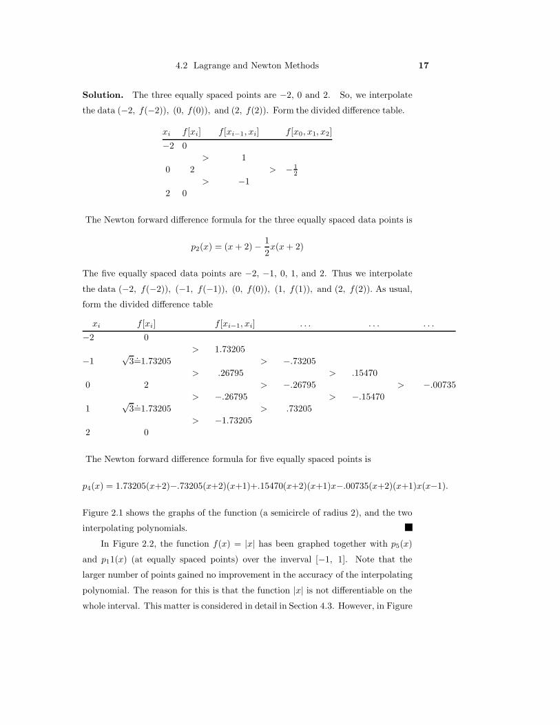
Solution. The three equally spaced points are −2, 0 and 2. So, we interpolate
the data (−2, f(−2)), (0, f(0)), and (2, f(2)). Form the divided difference table.
xi f [xi] f [xi−1, xi] f [x0, x1, x2]
−2 0> 1
0 2 > −12
> −12 0
The Newton forward difference formula for the three equally spaced data points is
p2(x) = (x + 2) − 12x(x + 2)
The five equally spaced data points are −2, −1, 0, 1, and 2. Thus we interpolate
the data (−2, f(−2)), (−1, f(−1)), (0, f(0)), (1, f(1)), and (2, f(2)). As usual,
form the divided difference table
xi f [xi] f [xi−1, xi] . . . . . . . . .
−2 0> 1.73205
−1√
3=̇1.73205 > −.73205> .26795 > .15470
0 2 > −.26795 > −.00735> −.26795 > −.15470
1√
3=̇1.73205 > .73205> −1.73205
2 0
The Newton forward difference formula for five equally spaced points is
p4(x) = 1.73205(x+2)−.73205(x+2)(x+1)+.15470(x+2)(x+1)x−.00735(x+2)(x+1)x(x−1).
Figure 2.1 shows the graphs of the function (a semicircle of radius 2), and the two
interpolating polynomials.
In Figure 2.2, the function f(x) = |x| has been graphed together with p5(x)
and p11(x) (at equally spaced points) over the inverval [−1, 1]. Note that the
larger number of points gained no improvement in the accuracy of the interpolating
polynomial. The reason for this is that the function |x| is not differentiable on the
whole interval. This matter is considered in detail in Section 4.3. However, in Figure

4.2 Lagrange and Newton Methods 18
2.3, the highly differentiable function f(x) = 3x2−sin 9x has been graphed together
with p5(x), p6(x), and p7(x) (at equally spaced points) over the interval [0,1]. Here
the approximants become better with an increasing number of points. Indeed, from
the methods of the next section it will become apparant that limn→∞ pn(x) = f(x),
for equally spaced points.
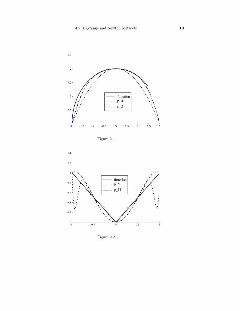
4.2 Lagrange and Newton Methods 19
Figure 2.1
Figure 2.2
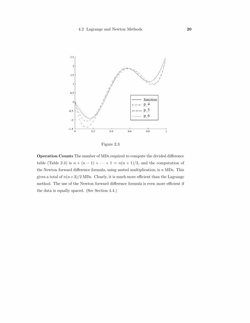
4.2 Lagrange and Newton Methods 20
Figure 2.3
Operation Counts The number of MDs required to compute the divided difference
table (Table 2.4) is n + (n − 1) + · · · + 1 = n(n + 1)/2, and the computation of
the Newton forward difference formula, using nested multiplication, is n MDs. This
gives a total of n(n+3)/2 MDs. Clearly, it is much more efficient than the Lagrange
method. The use of the Newton forward difference formula is even more efficient if
the data is equally spaced. (See Section 4.4.)

4.2 Lagrange and Newton Methods 21
4.2 Lagrange and Newton Methods 22
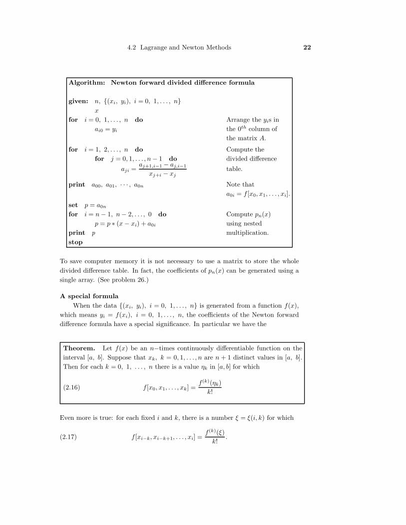
Algorithm: Newton forward divided difference formula
given: n, {(xi, yi), i = 0, 1, . . . , n}x
for i = 0, 1, . . . , n do Arrange the yis inai0 = yi the 0th column of
the matrix A.
for i = 1, 2, . . . , n do Compute thefor j = 0, 1, . . . , n − 1 do divided difference
aji =aj+1,i−1 − aj,i−1
xj+i − xjtable.
print a00, a01, · · · , a0n Note thata0i = f [x0, x1, . . . , xi].
set p = a0n
for i = n − 1, n − 2, . . . , 0 do Compute pn(x)p = p ∗ (x − xi) + a0i using nested
print p multiplication.stop
To save computer memory it is not necessary to use a matrix to store the wholedivided difference table. In fact, the coefficients of pn(x) can be generated using asingle array. (See problem 26.)
A special formulaWhen the data {(xi, yi), i = 0, 1, . . . , n} is generated from a function f(x),
which means yi = f(xi), i = 0, 1, . . . , n, the coefficients of the Newton forwarddifference formula have a special significance. In particular we have the
Theorem. Let f(x) be an n−times continuously differentiable function on theinterval [a, b]. Suppose that xk, k = 0, 1, . . . , n are n + 1 distinct values in [a, b].Then for each k = 0, 1, . . . , n there is a value ηk in [a, b] for which
(2.16) f [x0, x1, . . . , xk] =f(k)(ηk)
k!
Even more is true: for each fixed i and k, there is a number ξ = ξ(i, k) for which
(2.17) f [xi−k, xi−k+1, . . . , xi] =f(k)(ξ)
k!.
4.2 Lagrange and Newton Methods 23
See problem 27.This theorem, which will be proved in the next section, shows that the Newton
forward difference formula is similar the the Taylor Theorem, though the deriva-tives are evaluated at different points. It also shows that if the function f(x) is apolynomial of degree k, and k < n, then all the coefficients
(2.18) f [x0, x1, . . . , xk+1] = f [x0, x1, . . . , xk+2] = · · · = f [x0, x1, . . . , xn] = 0
4.2 Lagrange and Newton Methods 24
Exercises 4.2
In problems 1-6 find the Lagrange interpolating polynomial for the given data.
1. (0,1) (2,1) (3,2).
2. (−1, 1) (−2, 0) (2, 3).
3. (−1,−2) (0,−1) (1, 0) (2, 1).
4. (−5,−2) (−3, 1) (1, 7) (2, 1).
5. (4, 1) (2, 3) (−1, 2) (−3,−3).
6. (−1,−1) (6, 2) (4,−1) (1,−1).
In problems 7-12 find the coefficients of the Newton forward difference formula forthe given set of data.
7. (4, 5) (2, 3) (1,−1)
8. (−3, 3) (−1,−9) (4, 31)
9. (−2,−3) (−1,−7) (1,−9) (2, 65)
10. (−6, 1) (−1, 6) (1, 22) (5, 342)
11. (0,−1) (1, 0) (2,−1) (3, 2) (4, 15)
12. (−1, 5) (1, 13) (3, 45) (5, 53) (4, 25)
In problems 13-18 find the coefficients of the Newton backward difference formula.
13. (5,−2) (3, 4) (1, 2)
14. (1,−26) (−2, 1) (−1,−4) (4, 1)
15. (−4, 91) (−2,−3) (2, 1) (4, 3)
16. (−2, 10) (−1, 9) (0,−10) (9,−1)
17. (−1,−9) (0, 24) (1, 7) (2,−6) (8, 0)
18. (−2,−161) (−1,−89) (2,−5) (3,−1) (4, 1)
19. Find the Newton backward difference formula for the data {(kπ, sin kπ), i =0, 1, . . . , 7.
20. Find the Newton forward difference formula for the data {(k, k2), i = 0, 1, . . . , 6.
21. Suppose that p(x) is any polynomial of degree n, and that xi, i = 0, 1, . . . , n
are any n+1 distinct points. Show that the Newton forward difference formulapn(x) that interpolates the data {(xi, p(xi)), i = 0, 1, . . . , n} is equal to p(x)for all x.
4.2 Lagrange and Newton Methods 25
22. Given q(x), a polynomial of degree three. Suppose we interpolate five points{(xi, q(xi), i = 0, 1, . . . , 4}, where all the xis are distinct. Explain why infourth level divided difference f [x0, x1, . . . , x4] = 0.
23. Suppose you are given six points (xi, yi), i = 0, 1, . . . , 5, with all the xis aredistinct, and that there is a quadratic q(x) for which yi = q(xi), i = 0, 1, . . . , 6.How can the divided difference table be used to test this?
24. Suppose the data {(xi, yi), i = 0, 1, . . . , n} is given, and that {(x′i, y
′i), i =
0, 1, . . . , n} represents the exact same set of points. Show that if the divideddifference table is computed for both sets of data, then
f [x0, x1, . . . , xn] = f [x′1, x
′2, . . . , x
′n]
25. Find a formula to numerically compute the derivative of a polynomial pn(x) inNewton’s form. (See, formula (2.6))
26. Find an algorithm to compute the coefficients of the Newton forward differenceformula using only the two original data arrays. (Of course, the original y-datawill be lost.)
27. Verify formula (2.17).
28. Suppose that f(x) is a polynomial of degree k, and that xi, i = 0, 1, . . . , n arearbitrary and distinct. Show that if k < n, then (2.18) holds. (Note that theinterval [a, b] need not be specified because polynomials are defined for all x.
Computer ExercisesI Write a computer program to compute the coefficients of the Newton forward
difference formula for a given arbitrary set of data, and then to evaluate thepolynomial at specified points.
Applications: Use Program I to interpolate the following data.
1. (−32.00, 30.42) (19.00, 42.44) (20.00, 31.18)
2. (−12.15, 12.64) (−8.64, 6.76) (−7.02, 6.17) (−.54, 13.47) (.00,−10.14)(8.91, .81)
3. (−37.50, 12.64) (−30.75,−33.48) (−3.75, 7.56) (−3.00, 9.04)(−1.50, 32.53) (.00,−14.53) (.75, 21.38) (12.00,−30.72)
4. (−18.50, 9.69) (−14.80, 2.09) (−7.40,−1.26) (−2.96,−8.62) (1.85,−6.60)(2.96,−7.99) (10.36,−15.94) (11.47,−7.85) (12.95,−16.71) (16.28, 12.59)
5. Use Program I to interpolate the data {(2πk/8, sin 2πk/8), k = 0, 1, 2, . . . , 8}and then evaluate pn(x) at π/3. Compute also sin π/3.
4.2 Lagrange and Newton Methods 26
6. Use Program I to interpolate the data {(k, ek), k = 0, 1, 2, . . . , 6} and thenevaluate pn(x) at x = 5.5 and x = 8. Compute also e5.5 and e8.
II. Write a computer program to compute the coefficients of the Newtonbackward difference formula for a given arbitrary set of data, andthen to evaluate the polynomial at specified points. Applications:Use Program II to interpolate the following data.
Data to be inserted
III. Modify Program I to interpolate a given function at a specified set of orderednodes xi, i = 0, 1, . . . , n, and then to evaluate the interpolating polynomialat ten intermediate points to each pair [xi, xi+1]. Determine and print themaximum deviation from the polynomial to the function at these points.Applications: Use Program III to interpolate the given functions.
1. f(x) = 1/(1 + 5x2), xi = cos 2i+112 π, i = 0, 1, . . . , 5.
2. f(x) = 1/(1 + 5x2), xi = −1 + i10 , i = 0, 1, . . . , 10.
3. f(x) = |x|, xi = −2 + 2i8 , i = 0, 1, . . . , 8.
4. f(x) = 4x2 + sin 9x, xi = i2
64 , i = 0, 1, . . . , 8.
5. f(x) = 4x2 + sin 9x, xi = i8 , i = 0, 1, . . . , 8.
6. f(x) = 12(e−x − e−2x), xi = i10 , i = 0, 1, . . . , 10.
27
4.3 Error of the Interpolating Polynomial
In this section we suppose the data has the form {(xi, f(xi), i = 0, 1, . . . , n},for some given function f(x) that is n + 1—times continuously differentiable over
some interval. A natural question to ask is this: if pn(x) is the interpolating poly-
nomial for this data, and x is given, what is the difference
(3.1) f(x) − pn(x)
(Recall, Section 4.1, question 5.) We call this the error of approximation at x.
It is natural to expect this error to depend on three factors:
1. The given nodes, xi, i = 0, 1, . . . , n.
2. The selected value of x.
3. Properties of the function f(x).
For example, the further the value x is from the nodes, xi, i = 0, 1, . . . , n, the
greater the error of approximation might be. Or, the more the function oscillates,
the less representative of the function the data {(xi, f(xi), i = 0, 1, . . . , n} will
be and hence the greater the error of approximation. All of this is reflected in the
following theorem
Theorem. Error of Approximation. Assume that f(x) is continuous on the
interval [a, b] and (n + 1)−times continuously differentiable over (a, b), and that
the nodes xi, i = 0, 1, . . . , n are in [a, b]. Let pn(x) be the unique polynomial of
degree ≤ n that interpolates the data {(xi, f(xi), i = 0, 1, . . . , n}. Let x be some
fixed value in [a, b]. Then there is a value ξ in the smallest interval I that contains
the points {x, x0, x1, . . . , xn} for which
(3.2) f(x) − pn(x) =f(n+1)(ξ)(n + 1)!
(x − x0)(x − x1) · · · (x − xn)
where f(n+1)(x) denotes the (n + 1)st derivative of f(x).
4.3 Error of the Interpolating Polynomial 28
To verify this theorem we need a generalized version of Rolle’s theorem. First recall
the basic version of Rolle’s theorem: Suppose that g(x) is continuous on [a, b] and
differentiable on (a, b). If g(a) = g(b) = 0, then there is a value ξ in (a, b) for which
g′(ξ) = 0. This theorem generalizes to the situation when g(x) is zero at several
places in [a, b] as follows:
Theorem. Generalized Rolle’s Theorem. Suppose that g(x) is continuous
on [a, b] and (k + 1)− times continuously differentiable on (a, b). Suppose there
are k + 1 points xi, i = 0, 1, . . . , k in [a, b] at which g(x) is zero. That is,
g(xi) = 0, i = 0, 1, . . . , k. Then there is a number ξ in the smallest interval I that
contains the points xi, i = 0, 1, . . . , k at which
g(k)(ξ) = 0.
The proof of this theorem is really quite simple. First define the function
(3.3)
g(t) = f(t) − pn(t) −[
f(x) − pn(x)(x − x0)(x − x1) · · · (x − xn)
](t − x0)(t − x1) · · · (t − xn).
Note that g(t) is a function of the variable t — the number x is fixed! As a function
of t, we see that for t = xi,
g(xi) = f(xi) − pn(xi) −[
f(x) − pn(x)(x − x0)(x − x1) · · · (x − xn)
](xi − x0)(xi − x1) · · · (xi − xn)
= f(xi) − f(xi) −[
f(x) − pn(x)(x − x0)(x − x1) · · · (x − xn)
]· 0
= 0
for each xi, i = 0, 1, . . . , n. In addition, for t = x,
g(x) = f(x) − pn(x) −[
f(x) − pn(x)(x − x0)(x − x1) · · · (x − xn)
](x − x0)(x − x1) · · · (x − xn)
= f(x) − pn(x) − [f(x) − pn(x)]
= 0
Thus g(t) is zero at the n +2 points {x, x0, x1, . . . , xn}. By generalized Rolle’s theorem there must be a value
ξ in I, the smallest interval containing {x, x0, x1, . . . , xn} so that g(n+1)(ξ) = 0. Now compute the (n + 1)st
derivative of g(t).
dn+1
dtn+1g(t) =
dn+1
dtn+1f(t) − dn+1
dtn+1pn(t) −
[f(x) − pn(x)
(x − x0)(x − x1) · · · (x − xn)
]dn+1
dtn+1[(t − x0)(t − x1) · · · (t − xn)]
4.3 Error of the Interpolating Polynomial 29
Since pn(x) has degree ≤ n, dn+1
dtn+1 pn(t) = 0, for all t. On the other hand, the term
(t − x0)(t − x1) · · · (t − xn) is a polynomial of degree n + 1, which if expanded to
power form is
(t − x0)(t − x1) · · · (t − xn) = tn+1 + bntn + · · ·+ b0︸ ︷︷ ︸lower order terms
The (n + 1)st derivative of the lower order terms is 0. (Why?) Hence,
dn+1
dtn+1[(t − x0)(t − x1) · · · (t − xn)] =
dn+1
dtn+1tn+1 = (n + 1)!
Now evaluate at t = ξ obtained from the generalized Rolle’s theorem to get
0 = g(n+1)(ξ) = f(n+1)(ξ) −[
f(x) − pn(x)(x − x0)(x − x1) · · · (x − xn)
](n + 1)!
Finally, solving for f(x) − pn(x) we obtain the theorem
f(x) − pn(x) =f(n+1)(ξ)(n + 1)!
(x − x0)(x − x1) · · · (x − xn).
Example 3.1. Suppose f(x)+ex is to be interpolated at the points 0, 14, 1
2, 3
4, and 1.
What is the error of approximation at x = 13?
Solution. Five data points gives n = 4. Apply (3.2) with f(x) = ex. Then
f(5)(x) = ex. There exists some value ξ = ξ(13 ) such that
(3.4)e
13 − p4(
13) =
eξ
5!( 13−0)( 1
3− 14 )( 1
3− 12 )( 1
3− 34 )( 1
3−1)
=eξ
5!320125
As should be clear from (3.4) this error formula is not completely satisfactory,
because the number is ξ not explicitly known. All that is known is that ξ ε (0, 1).
This situation is almost identical to what happens in the Taylor theorem with
remainder. (See Chapter 1, Section 3.) By replacing the number f(n+1)(ξ) by
its maximum absolute value over the relevant interval I, we obtain a computable
estimate. Thus from (3.2) we have the more computable estimate
(3.5) |f(x) − pn(x)| ≤ maxξεI
∣∣f(n+1)(ξ)(n + 1)!
∣∣(x − x0)(x − x1) · · · (x − xn)|.
4.3 Error of the Interpolating Polynomial 30
Thus, for example, using (3.5) in (3.4) we obtain
(3.6)|e 1
3 − p4( 13 )| ≤ max
ξε(0,1)
∣∣eξ
5!
∣∣320125
=e1
5!320125
=̇.0000298
Still, the estimate (3.6) is not entirely satisfactory, because to use it the quantity
(x−x0)(x−x1) · · · (x−xn) must be calculated. Something simpler is desirable, and
when the nodes are equally spaced this product can be simply estimated. Recall,
that the n + 1 nodes are equally spaced over [a, b] if for h = (b − a)/n
(3.7)
x0 = a
x1 = a + h
...
xi = a + ih
...
xn = a + nh = b
It can be shown (See problem 11) that if x is in [a, b] then
(3.8) |(x − x0)(x − x1) · · · (x − xn)| ≤ 1
4hn+1n!
Putting the inequalities (3.4) and (3.8) together, we have
Error estimate for equally spaced data.
Suppose f(x) is continuous on [a, b] and n+1-times continuously differentiable over
the interval (a, b). If f(x) is interpolated at n + 1−equally spaced nodes given by
(3.7), where h = (b − a)/n, then, for any xε[a, b]
(3.9) |f(x) − pn(x)| ≤ hn+1
4(n + 1)max
ξε(a, b)|f(n+1)(ξ)|
Note that the factor1
n + 1in (3.9) comes from the multiplication of
1(n + 1)!
in (3.5)
by n! in (3.8). The error estimate (3.9) gives the maximum error possible. In most
cases the actual error is less. But note, with arbitrary nodes xi, i = 0, 1, . . . , n,
this estimate does not hold. We complete Example 3.1 in
4.3 Error of the Interpolating Polynomial 31
Example 3.2. Find an estimate for the error of approximation at any x in [0, 1]
incurred by interpolating ex at five equally spaced points in [0,1].
Solution. Here a = 0 and b = 1; so h = 1/4. As noted above f(5)(x) = ex is an
increasing function. Thus
maxξε(0, 1)
|f(5)(ξ)| = maxξε(0, 1)
eξ = e1 = e.
From (3.7),
|f(x) − p4(x)| ≤ (14 )5
4(5)e=̇.000133.
The approximation is quite good. The actual error is even smaller, about 5× 10⁻⁵.
The estimate (3.7) can also be used to determine how many equally spaced
point are required for an interpolating function to be accurate up to a specified
tolerance, say ε. This is accomplished by determining n so that the right hand side
of (3.7) is less than ε. That is,
To find the number of equally spaced points required for the error of interpolation
to be less than ε, solve the inequality
(3.10)hn+1
4(n + 1)max
ξε(a,b)|f(n+1)(ξ)| < ε.
for n.
Example 3.3. Given f(x) = 1x on [2, 4]. How many equally spaced points are
required so that the interpolating polynomial has an error of approximation less
than 10−5 on [2, 4]?
Solution. Since a = 2 and b = 4, h = (4 − 2)/n = 2/n. By (3.10), it is required
to solve the inequality
( 2n )n+1
4(n + 1)max
ξε(2, 4)|f(n+1)(ξ)| < 10−5.
4.3 Error of the Interpolating Polynomial 32
for n. The derivatives of f(x) =1x
are
f ′(x) = − 1x2
f ′′(x) =2x3
f ′′′(x) =−2 · 3
x4
...
f(n+1)(x) = (−1)n+1 (n + 1)!xn+2
Since the functions |f(n+1)(x)| are all decreasing, the maximum occurs at x = 2,
the left endpoint of the interval. Substitute in (3.10) above to get
( 2n )n+1
4(n + 1)(n + 1)!2n+2
< 10−5.
This simplifies ton!
8nn+1< 10−5
This inequality is difficult to solve for n directly, but we can construct a table of
values as follows:
nn!
8nn+1
8 3.7551× 10⁻⁵
9 1.3009× 10⁻⁵
10 4.5630× 10⁻⁶ < 10−5
The tolerance is met if 11 (= 10 + 1) equally spaced points are used.
Example 3.4. Consider f(x) = x−12 over the interval [1,3]. How many equally
spaced points are required for the error of interpolation to be less than 10−7?
Solution. Here a = 1 and b = 3; thus h = 2/n. Now compute the derivatives.
f(x) = x−12
f ′(x) = −12x−3
2
f ′′(x) =1 · 322
x− 52
f ′′′(x) = −1 · 3 · 523
x− 72
...
f(n+1)(x) = (−1)n+1 1 · 3 · 5 · · · (2n + 1)2n+1
x−2n+32
4.3 Error of the Interpolating Polynomial 33
Since the functions |f(n+1)(x)| are all decreasing, the maxima occur at x = 1.
Substituting all this into (3.10) we need to solve the equation
(2/n)n+1
4(n + 1)1 · 3 · 5 · · · (2n + 1)
2n+1=
(1/n)n
4n(n + 1)1 · 3 · 5 · · · (2n + 1) < 10−7
As in the previous example, construct a table:
n(1/n)n
4n(n + 1)1 · 3 · 5 · · · (2n + 1)
9 .00005910 .00002311 .000009 < 10−5
Hence, the tolerance is met if 12 (= 11 + 1) equally spaced points are used.
A special example
The foregoing discussion leads us to belive that the error of approximation for
an interpolating polynomial pn(x) to a given function f(x) can be made as small
as desired provided we use a sufficiently large number of equally spaced points.
The surprise is that this is not so. For some functions the error of approximation
increases with the number of equally spaced points. The best known example of
such a function is
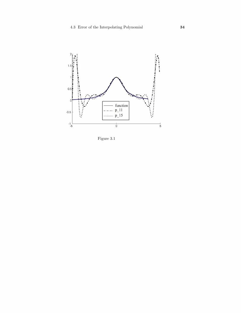
f(x) =1
1 + x2, −5 ≤ x ≤ 5.
In Figure 3.1 below we graph pn(x) for several values of n. Note that toward the
endpoints of the interval the error of approximation f(x) − pn(x) increases with n.
The reason for this is that the magnitudes of the derivatives become larger much
faster than the factors hn+1/(4(n + 1)) get small. Ways to avoid this have been
developed. It turns out that equally spaced data, though simple to compute, are the
wrong nodes to use. Indeed, other types of standard nodes will work. For example,
the Chebyshev points, which on [0,1] are defined by
(3.11) xn,i = cos2i + 12n + 2
π, i = i = 0, 1, . . . , n
can be used to approximate 1/(x2 + 1). The subscript n merely serves to indicate
that there is an infinite family of Chebyshev points, one for each value of n. However,
to prove that these nodes produce better results for this function would take us
beyond the scope of this book. The interested reader may consult the book by
Conte and de Boor [ ] for further information.
4.3 Error of the Interpolating Polynomial 34
Figure 3.1
4.3 Error of the Interpolating Polynomial 35
Exercises 4.3
In exercizes 1-8, for the given function and interval, determine the number of equally
spaced points that are required for the error of approximation of the interpolating
polynomial to be less than the given ε.
1. f(x) = sin 2x, [0, π], ε = 10−4
2. f(x) = cos 4x, [−π, π], ε = 10−5
3. f(x) = e2x, [1, 6], ε = 10−6
4. f(x) = e−x, [−4, 1], ε = 10−4
5. f(x) = 3 sin 2x− 2 cos 3x, [0, 2π], ε = 10−5
6. f(x) = 6 sin x − 5 sin 2x, [π, 3π], ε = 10−5
7. f(x) = 3√
x + 1, [1/2, 3/2], ε = 10−6
8. f(x) =√
3x, [1, 3], ε = 10−5
9. To illustrate how the size of the interval [a, b] and the magnitude of the deriva-
tives of the function f(x) affect the number of points needed to accurately
approximate the function, consider interpolating the function f(x) = sin cx,
over [a, b] with equally spaced points, where c, a, and b are given below. How
many equally spaced points are required to interpolate this function in order
that the error of approximation be less than ε = 10−5?
( a) c= 1, intervals [0,1], [0,5], and [0,10]
( b) c= 5, intervals [0,1], [0,5], and [0,10]
( c) c=10, intervals [0,1], [0,5], and [0,10]
10. At the end of Example 3.2 it was stated that the actual error of approximation
by the interpolating polynomial p4(x) was about 5 × 10⁻⁵. Outline a scheme
for determining this. (Do not actually do it!)
11. Give a verification of (3.8). (Hint. First find the subinterval(s) in which the left
hand side can be the biggest, and then find exactly where in those subintervals
the maximum occurs.)
12. Prove Generalized Rolle’s Theorem. (Hint. Use Rolle’s Theorem and mathe-
matical induction.)
36
4.4 Interpolation with Equally Spaced Data
In Section 4.2 the Newton forward and backward difference formulas were con-
structed for any type of data. However, naturally occuring or computed data if
often equally spaced. And as we noted in the previous section, the special case of
equally spaced data was somewhat simpler to work with. In this section we show
that for equally spaced data, the divided difference table becomes much simpler.
Moreover, the Newton forward and difference polynomials are simpler and cheaper
to compute. The key point is this: if the nodes are all equally spaced then the
denominators in each level of the divided difference table are simply calculated and
therefore need not be computed initially. Recall that the n + 1 nodes are called
equally spaced over [a, b] if for h = (b − a)/n
(4.1)
x0 = a
x1 = a + h
...
xi = a + ih
...
xn = a + nh = b
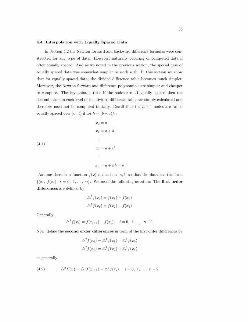
Assume there is a function f(x) defined on [a, b] so that the data has the form
{(xi, f(xi), i = 0, 1, . . . , n}. We need the following notation: The first order
differences are defined by
�1f(x0) = f(x1) − f(x0)
�1f(x1) = f(x2) − f(x1)
Generally,
�1f(xi) = f(xi+1) − f(xi), i = 0, 1, . . . , n − 1
Now, define the second order differences in term of the first order differences by
�2f(x0) = �1f(x1) −�1f(x0)
�2f(x1) = �1f(x2) −�1f(x1)
or generally
(4.2) �2f(xi) = �1f(xi+1) −�1f(xi), i = 0, 1, . . . , n − 2
4.4 Interpolation with Equally Spaced Data 37
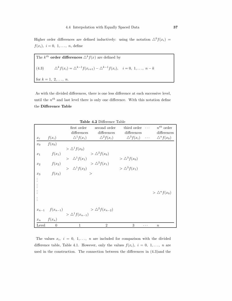
Higher order differences are defined inductively: using the notation �0f(xi) =
f(xi), i = 0, 1, . . . , n, define
The kth order differences �kf(x) are defined by
(4.3) �kf(xi) = �k−1f(xi+1) −�k−1f(xi), i = 0, 1, . . . , n − k
for k = 1, 2, . . . , n.
As with the divided differences, there is one less difference at each successive level,
until the nth and last level there is only one difference. With this notation define
the Difference Table
Table 4.2 Difference Table
first order second order third order · · · nth orderdifferences differences differences differences
xi f(xi) �1f(xi) �2f(xi) �3f(xi) · · · �nf(x0)
x0 f(x0)> �1f(x0)
x1 f(x1) > �2f(x0)> �1f(x1) > �3f(x0)
x2 f(x2) > �2f(x1)> �1f(x2) > �3f(x1)
x3 f(x3) >......... > �nf(x0)...
xn−1 f(xn−1) > �2f(xn−2)> �1f(xn−1)
xn f(xn)
Level 0 1 2 3 · · · n
The values xi, i = 0, 1, . . . , n are included for comparison with the divided
difference table, Table 4.1. However, only the values f(xi), i = 0, 1, . . . , n are
used in the construction. The connection between the differences in (4.3)and the
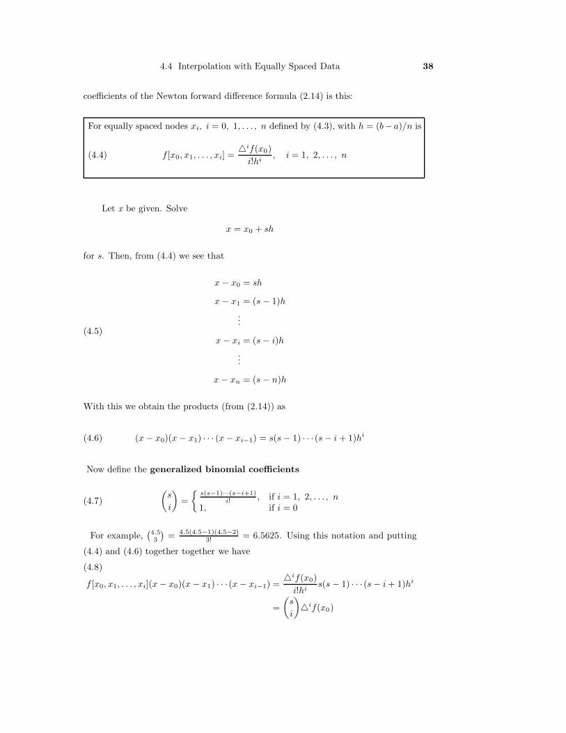
4.4 Interpolation with Equally Spaced Data 38
coefficients of the Newton forward difference formula (2.14) is this:
For equally spaced nodes xi, i = 0, 1, . . . , n defined by (4.3), with h = (b− a)/n is
(4.4) f [x0, x1, . . . , xi] =�if(x0)
i!hi, i = 1, 2, . . . , n
Let x be given. Solve
x = x0 + sh
for s. Then, from (4.4) we see that
(4.5)
x − x0 = sh
x − x1 = (s − 1)h...
x − xi = (s − i)h...
x − xn = (s − n)h
With this we obtain the products (from (2.14)) as
(4.6) (x − x0)(x − x1) · · · (x − xi−1) = s(s − 1) · · · (s − i + 1)hi
Now define the generalized binomial coefficients
(4.7)(
s
i
)=
{s(s−1)···(s−i+1)
i!, if i = 1, 2, . . . , n
1, if i = 0
For example,(4.53
)= 4.5(4.5−1)(4.5−2)
3!= 6.5625. Using this notation and putting
(4.4) and (4.6) together together we have
(4.8)
f [x0, x1, . . . , xi](x − x0)(x − x1) · · · (x − xi−1) =�if(x0)
i!his(s − 1) · · · (s − i + 1)hi
=(
s
i
)�if(x0)
4.4 Interpolation with Equally Spaced Data 39
Finally, with x = a + sh, the Newton forward difference formula has the form
The Newton forward difference formula for equally spaced data.
Given the equally spaced nodes given by (4.5), with x = a + sh, and with the gen-
eralized binomial coefficients given by (4.7), the Newton forward difference formula
is
(4.9) pn(x) = pn(a + sh) =n∑
i=0
(s
i
)�if(x0)
Note that in (4.9) the difference h has completely disappeared.
For equally spaced data the number of MD’s is especially small. The evaluation
of (4.9) requires only n + 1 MDs, once the numbers(
s
i
)have been evaluated, and
these values can be generated recursively, with 2 MDs for each. See problem .
Moreover, the difference table requires no MDs at all!
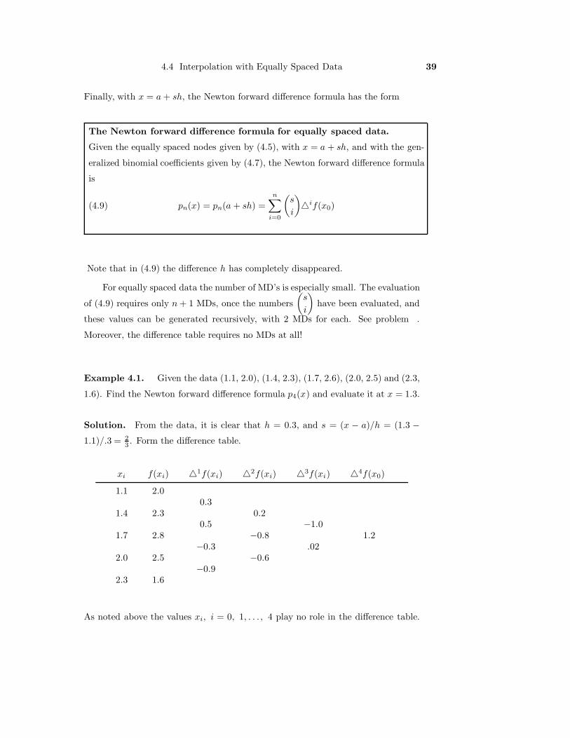
Example 4.1. Given the data (1.1, 2.0), (1.4, 2.3), (1.7, 2.6), (2.0, 2.5) and (2.3,
1.6). Find the Newton forward difference formula p4(x) and evaluate it at x = 1.3.
Solution. From the data, it is clear that h = 0.3, and s = (x − a)/h = (1.3 −1.1)/.3 = 2
3. Form the difference table.
xi f(xi) �1f(xi) �2f(xi) �3f(xi) �4f(x0)
1.1 2.00.3
1.4 2.3 0.20.5 −1.0
1.7 2.8 −0.8 1.2−0.3 .02
2.0 2.5 −0.6−0.9
2.3 1.6
As noted above the values xi, i = 0, 1, . . . , 4 play no role in the difference table.
4.4 Interpolation with Equally Spaced Data 40
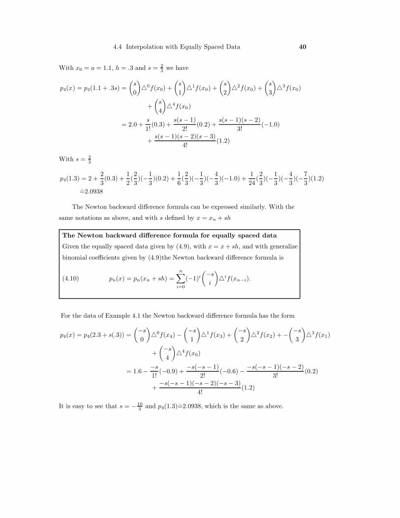
With x0 = a = 1.1, h = .3 and s = 23 we have
p4(x) = p4(1.1 + .3s) =(
s
0
)�0f(x0) +
(s
1
)�1f(x0) +
(s
2
)�2f(x0) +
(s
3
)�3f(x0)
+(
s
4
)�4f(x0)
= 2.0 +s
1!(0.3) +
s(s − 1)2!
(0.2) +s(s − 1)(s − 2)
3!(−1.0)
+s(s − 1)(s− 2)(s − 3)
4!(1.2)
With s = 23
p4(1.3) = 2 +23(0.3) +
12(23)(−1
3)(0.2) +
16(23)(−1
3)(−4
3)(−1.0) +
124
(23)(−1
3)(−4
3)(−7
3)(1.2)
=̇2.0938
The Newton backward difference formula can be expressed similarly. With the
same notations as above, and with s defined by x = xn + sh
The Newton backward difference formula for equally spaced data
Given the equally spaced data given by (4.9), with x = x + sh, and with generalize
binomial coefficients given by (4.9)the Newton backward difference formula is
(4.10) pn(x) = pn(xn + sh) =n∑
i=0
(−1)i
(−s
i
)�if(xn−i).
For the data of Example 4.1 the Newton backward difference formula has the form
p4(x) = p4(2.3 + s(.3)) =(−s
0
)�0f(x4) −
(−s
1
)�1f(x3) +
(−s
2
)�2f(x2) + −
(−s
3
)�3f(x1)
+(−s
4
)�4f(x0)
= 1.6− −s
1!(−0.9) +
−s(−s − 1)2!
(−0.6) − −s(−s − 1)(−s − 2)3!
(0.2)
+−s(−s − 1)(−s − 2)(−s − 3)
4!(1.2)
It is easy to see that s = −103 and p4(1.3)=̇2.0938, which is the same as above.
4.4 Interpolation with Equally Spaced Data 41
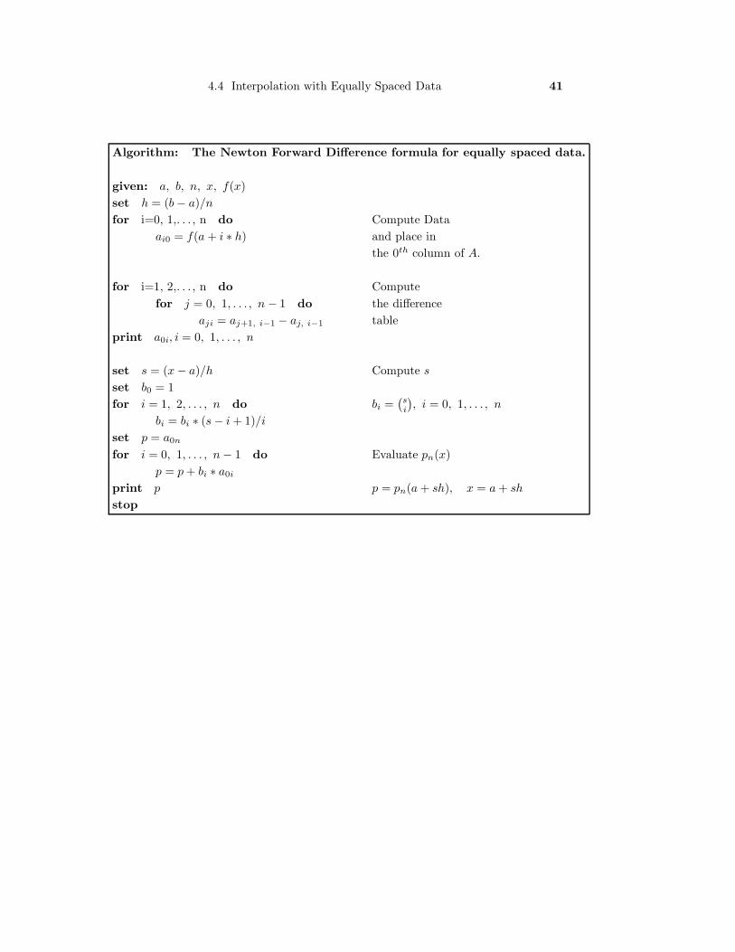
Algorithm: The Newton Forward Difference formula for equally spaced data.
given: a, b, n, x, f(x)set h = (b − a)/n
for i=0, 1,. . . , n do Compute Dataai0 = f(a + i ∗ h) and place in
the 0th column of A.
for i=1, 2,. . . , n do Computefor j = 0, 1, . . . , n − 1 do the difference
aji = aj+1, i−1 − aj, i−1 tableprint a0i, i = 0, 1, . . . , n
set s = (x − a)/h Compute s
set b0 = 1for i = 1, 2, . . . , n do bi =
(si
), i = 0, 1, . . . , n
bi = bi ∗ (s − i + 1)/i
set p = a0n
for i = 0, 1, . . . , n − 1 do Evaluate pn(x)p = p + bi ∗ a0i
print p p = pn(a + sh), x = a + sh
stop
4.4 Interpolation with Equally Spaced Data 42
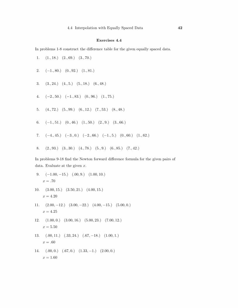
Exercises 4.4
In problems 1-8 construct the difference table for the given equally spaced data.
1. (1., 18.) (2., 69.) (3., 70.)
2. (−1., 80.) (0., 92.) (1., 81.)
3. (3., 24.) (4., 5.) (5., 18.) (6., 48.)
4. (−2., 50.) (−1., 83.) (0., 96.) (1., 75.)
5. (4., 72.) (5., 99.) (6., 12.) (7., 53.) (8., 48.)
6. (−1., 51.) (0., 46.) (1., 50.) (2., 9.) (3., 66.)
7. (−4., 45.) (−3., 0.) (−2., 66.) (−1., 5.) (0., 60.) (1., 62.)
8. (2., 93.) (3., 30.) (4., 78.) (5., 9.) (6., 85.) (7., 42.)
In problems 9-18 find the Newton forward difference formula for the given pairs of
data. Evaluate at the given x.
9. (−1.00,−15.) (.00, 9.) (1.00, 10.)
x = .70
10. (3.00, 15.) (3.50, 21.) (4.00, 15.)
x = 4.20
11. (2.00,−12.) (3.00,−22.) (4.00,−15.) (5.00, 0.)
x = 4.25
12. (1.00, 0.) (3.00, 16.) (5.00, 23.) (7.00, 12.)
x = 5.50
13. (.00, 11.) (.33, 24.) (.67,−18.) (1.00, 1.)
x = .60
14. (.00, 0.) (.67, 0.) (1.33,−1.) (2.00, 0.)
x = 1.60
4.4 Interpolation with Equally Spaced Data 43
15. (.00,−20.) (.70, 8.) (1.40,−2.) (2.10,−24.)
x = 1.60
16. (−3.00, 8.) (−2.01,−22.) (−1.02, 5.) (−.03, 6.)
x = .00
17. (1.00, 21.) (2.00,−9.) (3.00, 14.) (4.00,−20.) (5.00, 17.)
x = 3.80
18. (−2.00,−3.) (−1.00,−24.) (.00, 4.) (1.00, 15.) (2.00, 2.)
x = −1.40
In problem 19-26 find the Newton backward difference formula for the given data.
Evaluate at the given value of x.
19. (3.00,−15.) (5.00, 9.) (7.00, 10.)
x = 5.50
20. (.00, 15.) (1.00, 21.) (2.00, 15.)
x = 1.50
21. (1.00,−12.) (2.00,−22.) (3.00,−15.) (4.00, 0.)
x = 2.50
22. (−3.00, 0.) (−1.00, 16.) (1.00, 23.) (3.00, 12.)
x = .50
23. (.00, 11.) (1.00, 24.) (2.00,−18.) (3.00, 1.) (4.00, 0.)
x = 1.60
24. (3.00, 0.) (5.00,−1.) (7.00, 0.) (9.00,−20.) (11.00, 8.)
x = 2.00
25. (1.00,−2.) (1.25,−24.) (1.50, 8.) (1.75,−22.) (2.00, 5.)
x = 1.60
26. (−5.00, 6.) (−2.50, 21.) (.00,−9.) (2.50, 14.) (5.00,−20.)
x = 3.50
27. Find the Newton forward difference formula for the equally spaced data given
by
{(i/5, sin 2πi/5), i = 0, 1, . . . , 5}. Evaluate at x = .70.
4.4 Interpolation with Equally Spaced Data 44
28. Find the Newton forward difference formula for the equally spaced data given
by
{(i/4, cos 2πi/4), i = 0, 1, . . . , 4}. Evaluate at x = .30.
29. Find the Newton forward difference formula for the equally spaced data given
by
1.7 to 2.1 ,with h = .1 and f(x) = e2x. Evaluate at x = 1.60.
30. Find the Newton forward difference formula for the equally spaced data given
by
−2.0 to 3.0 ,with h = 1. and f(x) = e−3x. Evaluate at x = −1.50.
31. Find the Newton forward difference formula for the equally spaced data given
by
1.0 to 3.0, with h = .5 and f(x) = lnx. Evaluate at x = 1.40.
32. Find the Newton forward difference formula for the equally spaced data given
by
−1.0 to 1.0. with h = .5 and f(x) = 11+25x2 . Evaluate at x = .90.
33. Show what simplifications can be made the the Lagrange interpolating poly-
nomial for equally spaced data.
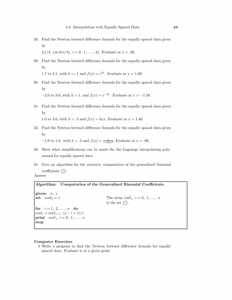
34. Give an algorithm for the recursive computation of the generalized binomial
coefficients(si
).
Answer
Algorithm: Computation of the Generalized Binomial Coefficients
given: n, sset coef0 = 1 The array coef i, i = 0, 1, . . . , n
is the set(si
).
for i = 1, 2, . . . , n docoef i = coef i−1 · (s − i + 1)/iprint coef i, i = 0, 1, . . . , nstop
Computer ExercisesI Write a program to find the Newton forward difference formula for equally
spaced data. Evaluate it at a given point.

4.4 Interpolation with Equally Spaced Data 45
Applications.
Data to be inserted
II Write a program to find the Newton backward difference formula for equallyspaced data. Evaluate it at a given point.Applications.
Data to be inserted
46
4.5 Interpolation with Cubic Splines
When dealing with large volumes of data, or when the interpolating polynomial
exibits large internodal fluctuations, standard Newton or Lagrange interpolation
may not be the best way to approximate functions. In this section we introduce an
alternative method for approximating functions.
In some ways, this new method is based more upon the idea of representing a
function in the sense of description, than that of interpolation per se. Moreover,
this alternative is simple in concept, really no more difficult that the connect the dot
drawings for children. We continue to use polynomials, but the new feature is that
a distinct polynomials are computed for each successive pair of nodes. For example,
in Figure 5.1 (a) and (b), observe that the data is represented on the graphs by
straight lines. This first, Figure 5.1(a), is commonly called a bar graph. Widely
used in industry and government, it is an effective means of simply representing
data without any hint of trends. It is ususally used when data has been summed,
averaged, or otherwise lumped together over various time periods. The second,
Figure 5.1(b), shows data points connected by straight lines. Graphs of this sort
are usually used when the some interpretation of the function at internodal points
is desired. The 30-day Dow-Jones stock averages are reported in this way. Both
graphs have the common feature that between nodes the curve is a polynomial, of
degree 0 in Figure 5.1(a) and degree 1 in Figure 5.1(b). Note that a different line
is used between successive nodes. Both these curves are called piecewise linear
polynomials although the first is also called a piecewise constant curve. Another
way to describe the difference between them is that in Figure 5.1(b) the straight
lines are selected to match, or be equal, at the nodes, while in (a) this is not required.
So when developing this alternative method we must decide what degree polynomial
to use between nodes, and how well the ”pieced together” polynomials must match
up at the nodes.
Let us make our notions precise. Suppose we are given the data {(xi, yi), i =
0, 1, . . . , n}, where we assume now and thoughout this section that x0 < x1 < x2 <
· · · < xn. Suppose that S0(x) is a polynomial defined on [x0, x1) which satisfies
S0(x0) = y0. Similarly, let Si(x) i = 1, 2, . . . , n − 1, denote polynomials defined
4.5 Interpolation with Cubic Splines 47
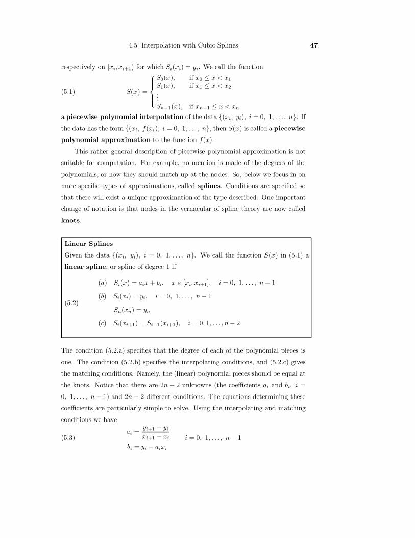
respectively on [xi, xi+1) for which Si(xi) = yi. We call the function
(5.1) S(x) =
⎧⎪⎪⎨⎪⎪⎩
S0(x), if x0 ≤ x < x1
S1(x), if x1 ≤ x < x2
...Sn−1(x), if xn−1 ≤ x < xn
a piecewise polynomial interpolation of the data {(xi, yi), i = 0, 1, . . . , n}. If
the data has the form {(xi, f(xi), i = 0, 1, . . . , n}, then S(x) is called a piecewise
polynomial approximation to the function f(x).
This rather general description of piecewise polynomial approximation is not
suitable for computation. For example, no mention is made of the degrees of the
polynomials, or how they should match up at the nodes. So, below we focus in on
more specific types of approximations, called splines. Conditions are specified so
that there will exist a unique approximation of the type described. One important
change of notation is that nodes in the vernacular of spline theory are now called
knots.
Linear Splines
Given the data {(xi, yi), i = 0, 1, . . . , n}. We call the function S(x) in (5.1) a
linear spline, or spline of degree 1 if
(5.2)
(a) Si(x) = aix + bi, x ε [xi, xi+1], i = 0, 1, . . . , n − 1
(b) Si(xi) = yi, i = 0, 1, . . . , n − 1
Sn(xn) = yn
(c) Si(xi+1) = Si+1(xi+1), i = 0, 1, . . . , n− 2
The condition (5.2.a) specifies that the degree of each of the polynomial pieces is
one. The condition (5.2.b) specifies the interpolating conditions, and (5.2.c) gives
the matching conditions. Namely, the (linear) polynomial pieces should be equal at
the knots. Notice that there are 2n − 2 unknowns (the coefficients ai and bi, i =
0, 1, . . . , n − 1) and 2n − 2 different conditions. The equations determining these
coefficients are particularly simple to solve. Using the interpolating and matching
conditions we have
(5.3)ai =
yi+1 − yi
xi+1 − xi
bi = yi − aixi
i = 0, 1, . . . , n − 1
4.5 Interpolation with Cubic Splines 48
The equations (5.3) completely determine the linear spline. Moreover, it is unique.
As indicated above, for some applications linear splines are good enough. If, for
example, the data is only known approximately, very little more can be achieved
by using higher order polynomials. An example of a linear spline is given by Figure
5.1b.
Example 5.1. Find the linear spline that interpolates the data (−1, 2), (1, 4), (2, 4),
and (3,1). Graph the spline and evaluate it at x = 2.5.
Solution. The number of data points is four. So, with n = 3, we see that there
are three linear pieces to determine, S0(x), S1(x), and S2(x). From (5.3) we have
that
a0 =4 − 2
1 − (−1)= 2
a1 =4 − 42 − 1
= 0
a2 =1 − 43 − 2
= −3
b0 = 2 − 2(−1) = 4
b1 = 4 − 0(1) = 4
b2 = 4 − (−3)(2) = 10
Thus
S0(x) = 2x + 4
S1(x) = 4
S2(x) = −3x + 10
Since x = 2.5 lies between x2 = 2 and x3 = 3, we compute S(2.5) using S2(x).
S2(2.5) = −3(2.5) + 10 = 2.5
The graph is shown in Figure 5.2.
More important from the viewpoint of approximation accuracy and visual ap-
pearance are the cubic splines, which are defined below.
4.5 Interpolation with Cubic Splines 49
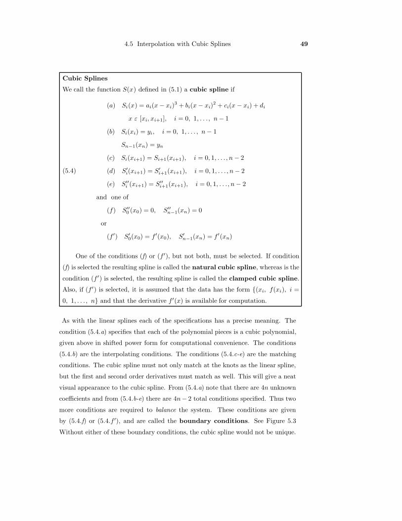
Cubic Splines
We call the function S(x) defined in (5.1) a cubic spline if
(5.4)
(a) Si(x) = ai(x − xi)3 + bi(x − xi)2 + ci(x − xi) + di
x ε [xi, xi+1], i = 0, 1, . . . , n − 1
(b) Si(xi) = yi, i = 0, 1, . . . , n − 1
Sn−1(xn) = yn
(c) Si(xi+1) = Si+1(xi+1), i = 0, 1, . . . , n − 2
(d) S′i(xi+1) = S′
i+1(xi+1), i = 0, 1, . . . , n − 2
(e) S′′i (xi+1) = S′′
i+1(xi+1), i = 0, 1, . . . , n − 2
and one of
(f) S′′0 (x0) = 0, S′′
n−1(xn) = 0
or
(f ′) S′0(x0) = f ′(x0), S′
n−1(xn) = f ′(xn)
One of the conditions (f) or (f ′), but not both, must be selected. If condition
(f) is selected the resulting spline is called the natural cubic spline, whereas is the
condition (f ′) is selected, the resulting spline is called the clamped cubic spline.
Also, if (f ′) is selected, it is assumed that the data has the form {(xi, f(xi), i =
0, 1, . . . , n} and that the derivative f ′(x) is available for computation.
As with the linear splines each of the specifications has a precise meaning. The
condition (5.4.a) specifies that each of the polynomial pieces is a cubic polynomial,
given above in shifted power form for computational convenience. The conditions
(5.4.b) are the interpolating conditions. The conditions (5.4.c-e) are the matching
conditions. The cubic spline must not only match at the knots as the linear spline,
but the first and second order derivatives must match as well. This will give a neat
visual appearance to the cubic spline. From (5.4.a) note that there are 4n unknown
coefficients and from (5.4.b-e) there are 4n− 2 total conditions specified. Thus two
more conditions are required to balance the system. These conditions are given
by (5.4.f) or (5.4.f ′), and are called the boundary conditions. See Figure 5.3
Without either of these boundary conditions, the cubic spline would not be unique.
4.5 Interpolation with Cubic Splines 50
We state the following theorem, without proof.
Theorem. The natural or clamped cubic spline defined above is unique.
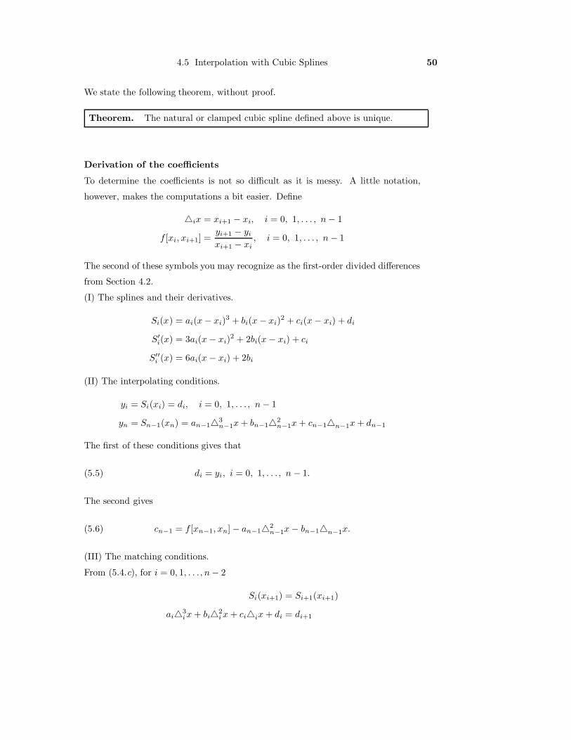
Derivation of the coefficients
To determine the coefficients is not so difficult as it is messy. A little notation,
however, makes the computations a bit easier. Define
�ix = xi+1 − xi, i = 0, 1, . . . , n − 1
f [xi, xi+1] =yi+1 − yi
xi+1 − xi, i = 0, 1, . . . , n − 1
The second of these symbols you may recognize as the first-order divided differences
from Section 4.2.
(I) The splines and their derivatives.
Si(x) = ai(x − xi)3 + bi(x − xi)2 + ci(x − xi) + di
S′i(x) = 3ai(x − xi)2 + 2bi(x − xi) + ci
S′′i (x) = 6ai(x − xi) + 2bi
(II) The interpolating conditions.
yi = Si(xi) = di, i = 0, 1, . . . , n − 1
yn = Sn−1(xn) = an−1�3n−1x + bn−1�2
n−1x + cn−1�n−1x + dn−1
The first of these conditions gives that
(5.5) di = yi, i = 0, 1, . . . , n − 1.
The second gives
(5.6) cn−1 = f [xn−1, xn] − an−1�2n−1x − bn−1�n−1x.
(III) The matching conditions.
From (5.4.c), for i = 0, 1, . . . , n − 2
Si(xi+1) = Si+1(xi+1)
ai�3i x + bi�2
i x + ci�ix + di = di+1
4.5 Interpolation with Cubic Splines 51
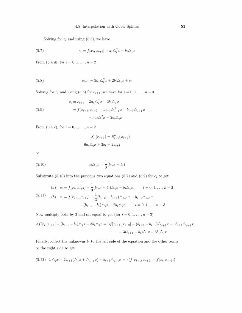
Solving for ci and using (5.5), we have
(5.7) ci = f [xi, xi+1] − ai�2i x − bi�ix
From (5.4.d), for i = 0, 1, . . . , n − 2
(5.8) ci+1 = 3ai�2i x + 2bi�ix + ci
Solving for ci and using (5.8) for ci+1, we have for i = 0, 1, . . . , n− 3
(5.9)
ci = ci+1 − 3ai�2i x − 2bi�ix
= f [xi+1, xi+2] − ai+1�2i+1x − bi+1�i+1x
− 3ai�2i x − 2bi�ix
From (5.4.e), for i = 0, 1, . . . , n − 2
S′′i (xi+1) = S′′
i+1(xi+1)
6ai�ix + 2bi = 2bi+1
or
(5.10) ai�ix =13(bi+1 − bi)
Substitute (5.10) into the previous two equations (5.7) and (5.9) for ci to get
(5.11)
(a) ci = f [xi, xi+1] − 13(bi+1 − bi)�ix − bi�ix, i = 0, 1, . . . , n− 2
(b) ci = f [xi+1, xi+2] − 13(bi+2 − bi+1)�i+1x − bi+1�i+1x
− (bi+1 − bi)�ix − 2bi�ix, i = 0, 1, . . . , n − 3
Now multiply both by 3 and set equal to get (for i = 0, 1, . . . , n − 3)
3f [xi, xi+1]− (bi+1 − bi)�ix − 3bi�ix = 3f [xi+1, xi+2] − (bi+2 − bi+1)�i+1x − 3bi+1�i+1x
− 3(bi+1 − bi)�ix − 6bi�ix
Finally, collect the unknowns bi to the left side of the equation and the other terms
to the right side to get
(5.12) bi�ix + 2bi+1(�ix + �i+1x) + bi+2�i+1x = 3(f [xi+1, xi+2] − f [xi, xi+1])
4.5 Interpolation with Cubic Splines 52
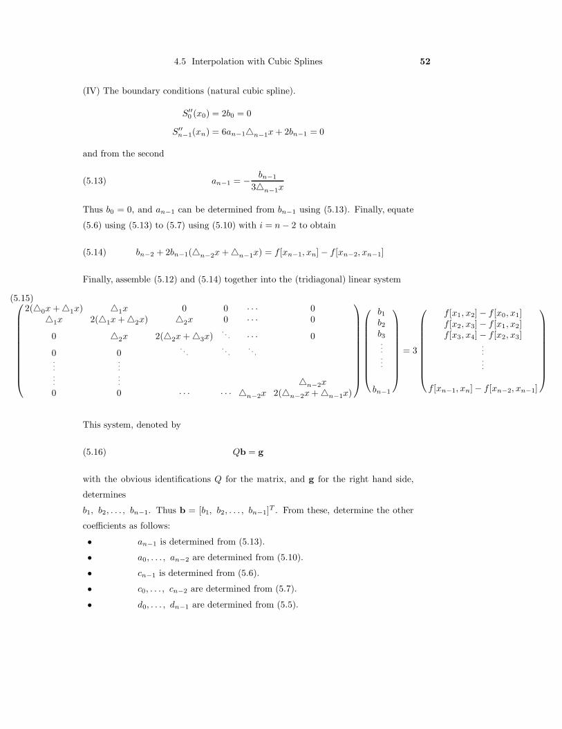
(IV) The boundary conditions (natural cubic spline).
S′′0 (x0) = 2b0 = 0
S′′n−1(xn) = 6an−1�n−1x + 2bn−1 = 0
and from the second
(5.13) an−1 = − bn−1
3�n−1x
Thus b0 = 0, and an−1 can be determined from bn−1 using (5.13). Finally, equate
(5.6) using (5.13) to (5.7) using (5.10) with i = n − 2 to obtain
(5.14) bn−2 + 2bn−1(�n−2x + �n−1x) = f [xn−1, xn] − f [xn−2, xn−1]
Finally, assemble (5.12) and (5.14) together into the (tridiagonal) linear system
(5.15)⎛⎜⎜⎜⎜⎜⎜⎜⎜⎜⎜⎜⎝
2(�0x + �1x) �1x 0 0 · · · 0�1x 2(�1x + �2x) �2x 0 · · · 0
0 �2x 2(�2x + �3x). . . · · · 0
0 0. . .
. . .. . .
.
.
....
.
.
.... �n−2x
0 0 · · · · · · �n−2x 2(�n−2x + �n−1x)
⎞⎟⎟⎟⎟⎟⎟⎟⎟⎟⎟⎟⎠
⎛⎜⎜⎜⎜⎜⎜⎜⎜⎜⎝
b1
b2
b3......
bn−1
⎞⎟⎟⎟⎟⎟⎟⎟⎟⎟⎠
= 3
⎛⎜⎜⎜⎜⎜⎜⎜⎜⎜⎝
f [x1, x2] − f [x0, x1]f [x2, x3] − f [x1, x2]f [x3, x4] − f [x2, x3]
.
.
.
.
.
.
f [xn−1, xn]− f [xn−2, xn−1]
⎞⎟⎟⎟⎟⎟⎟⎟⎟⎟⎠
This system, denoted by
(5.16) Qb = g
with the obvious identifications Q for the matrix, and g for the right hand side,
determines
b1, b2, . . . , bn−1. Thus b = [b1, b2, . . . , bn−1]T . From these, determine the other
coefficients as follows:
• an−1 is determined from (5.13).
• a0, . . . , an−2 are determined from (5.10).
• cn−1 is determined from (5.6).
• c0, . . . , cn−2 are determined from (5.7).
• d0, . . . , dn−1 are determined from (5.5).
4.5 Interpolation with Cubic Splines 53
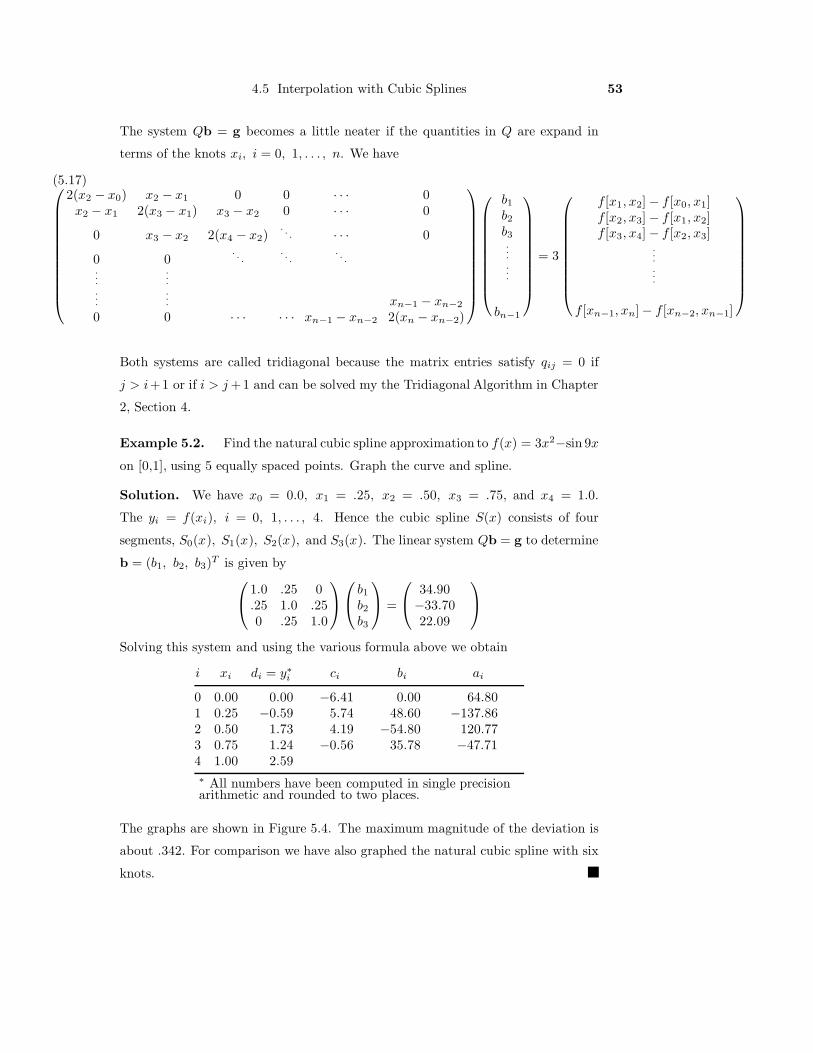
The system Qb = g becomes a little neater if the quantities in Q are expand in
terms of the knots xi, i = 0, 1, . . . , n. We have
(5.17)⎛⎜⎜⎜⎜⎜⎜⎜⎜⎜⎜⎜⎝
2(x2 − x0) x2 − x1 0 0 · · · 0x2 − x1 2(x3 − x1) x3 − x2 0 · · · 0
0 x3 − x2 2(x4 − x2). . . · · · 0
0 0. . .
. . .. . .
.
.
....
.
.
.... xn−1 − xn−2
0 0 · · · · · · xn−1 − xn−2 2(xn − xn−2)
⎞⎟⎟⎟⎟⎟⎟⎟⎟⎟⎟⎟⎠
⎛⎜⎜⎜⎜⎜⎜⎜⎜⎜⎝
b1
b2
b3......
bn−1
⎞⎟⎟⎟⎟⎟⎟⎟⎟⎟⎠
= 3
⎛⎜⎜⎜⎜⎜⎜⎜⎜⎜⎝
f [x1, x2] − f [x0, x1]f [x2, x3] − f [x1, x2]f [x3, x4] − f [x2, x3]
.
.
.
.
.
.
f [xn−1, xn]− f [xn−2, xn−1]
⎞⎟⎟⎟⎟⎟⎟⎟⎟⎟⎠
Both systems are called tridiagonal because the matrix entries satisfy qij = 0 if
j > i+1 or if i > j +1 and can be solved my the Tridiagonal Algorithm in Chapter
2, Section 4.
Example 5.2. Find the natural cubic spline approximation to f(x) = 3x2−sin 9x
on [0,1], using 5 equally spaced points. Graph the curve and spline.
Solution. We have x0 = 0.0, x1 = .25, x2 = .50, x3 = .75, and x4 = 1.0.
The yi = f(xi), i = 0, 1, . . . , 4. Hence the cubic spline S(x) consists of four
segments, S0(x), S1(x), S2(x), and S3(x). The linear system Qb = g to determine
b = (b1, b2, b3)T is given by⎛⎝ 1.0 .25 0
.25 1.0 .250 .25 1.0
⎞⎠
⎛⎝ b1
b2
b3
⎞⎠ =
⎛⎝ 34.90
−33.7022.09
⎞⎠
Solving this system and using the various formula above we obtain
i xi di = y∗i ci bi ai
0 0.00 0.00 −6.41 0.00 64.801 0.25 −0.59 5.74 48.60 −137.862 0.50 1.73 4.19 −54.80 120.773 0.75 1.24 −0.56 35.78 −47.714 1.00 2.59∗ All numbers have been computed in single precisionarithmetic and rounded to two places.
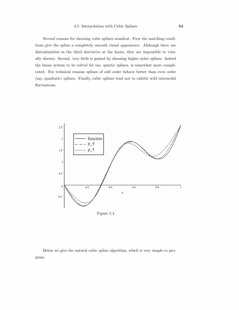
The graphs are shown in Figure 5.4. The maximum magnitude of the deviation is
about .342. For comparison we have also graphed the natural cubic spline with six
knots.
4.5 Interpolation with Cubic Splines 54
Several reasons for choosing cubic splines standout. First the matching condi-
tions give the spline a completely smooth visual appearence. Although there are
discontinuities in the third derivative at the knots, they are impossible to visu-
ally discern. Second, very little is gained by choosing higher order splines. Indeed
the linear system to be solved for say, quartic splines, is somewhat more compli-
cated. For technical reasons splines of odd order behave better than even order
(say, quadratic) splines. Finally, cubic splines tend not to exhibit wild internodal
fluctuations.
Figure 5.4
Below we give the natural cubic spline algorithm, which is very simple to pro-
gram.
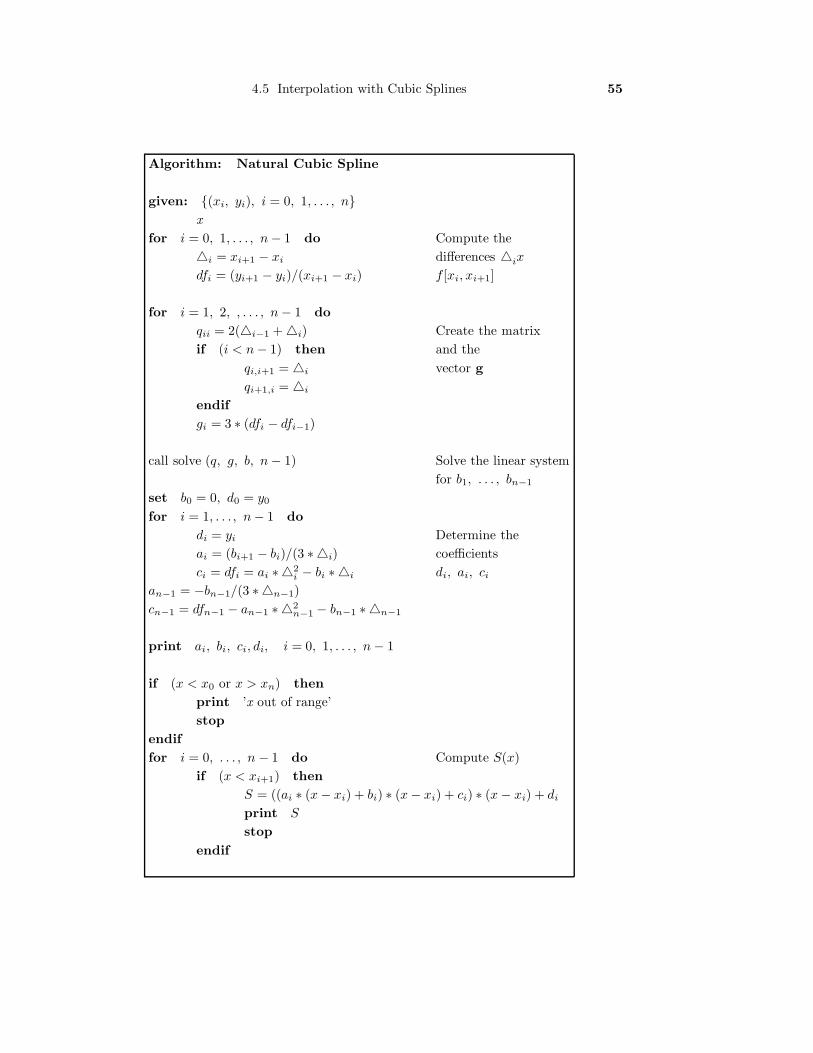
4.5 Interpolation with Cubic Splines 55
Algorithm: Natural Cubic Spline
given: {(xi, yi), i = 0, 1, . . . , n}x
for i = 0, 1, . . . , n − 1 do Compute the�i = xi+1 − xi differences �ix
dfi = (yi+1 − yi)/(xi+1 − xi) f [xi, xi+1]
for i = 1, 2, , . . . , n − 1 doqii = 2(�i−1 + �i) Create the matrixif (i < n − 1) then and the
qi,i+1 = �i vector gqi+1,i = �i
endifgi = 3 ∗ (dfi − dfi−1)
call solve (q, g, b, n − 1) Solve the linear systemfor b1, . . . , bn−1
set b0 = 0, d0 = y0
for i = 1, . . . , n − 1 dodi = yi Determine theai = (bi+1 − bi)/(3 ∗ �i) coefficientsci = dfi = ai ∗ �2
i − bi ∗ �i di, ai, ci
an−1 = −bn−1/(3 ∗ �n−1)cn−1 = dfn−1 − an−1 ∗ �2
n−1 − bn−1 ∗ �n−1
print ai, bi, ci, di, i = 0, 1, . . . , n − 1
if (x < x0 or x > xn) thenprint ’x out of range’stop
endiffor i = 0, . . . , n − 1 do Compute S(x)
if (x < xi+1) thenS = ((ai ∗ (x − xi) + bi) ∗ (x − xi) + ci) ∗ (x − xi) + di
print S
stopendif

4.5 Interpolation with Cubic Splines 56
In the cubic spline algorithm above, the system can be replace by the tridiagonal
algorithm from Chapter 3.
4.5 Interpolation with Cubic Splines 57
Exercises 4.5
In problems 1-6 determine the linear splines that interpolates the given data.
1. (1, 0) (2,−3) (3,−1) (4, 1)
2. (−2, 0) (0, 10) (1, 13) (2, 10)
3. (0, 0) (2,−6) (3,−6) (5,−6) (7, 2)
4. (−3, 0) (−1, 6) (0, 8) (4, 28) (6, 20)
5. (−2, 0) (−1, 0) (0, 0) (1, 0) (2, 0) (3,−4)
6. (−4, 0) (−2, 0) (−1,−5) (2, 1) (3,−4) (5,−2)
In problems 7-12 determine the coefficients of the natural cubic spline that inter-
polates the given data.
7. (0, 1) (1, 1) (2,−3)
8. (−1,−1) (1, 17) (3, 99)
9. (1, 0) (2,−1) (3,−5) (4,−6)
10. (−2, 2) (0, 12) (2, 46) (4, 56)
11. (0, 0) (2, 0) (4, 0) (6,−16) (8,−96)
12. (−2, 1) (−1,−1) (0,−5) (1,−19) (2,−43)
13. Find the matrix Q when the data is equally spaced. (Assume that xi+1 − xi =
h, i = 0, 1, . . . , n − 1.)
14. Define the linear spline the same as (5.2) replacing (5.2a) with Si(x) = ai(x −xi) + bi over the same range of x and i. Determine the coefficients ai, bi, i =
0, 1, . . . , n − 1.
15. If the data has the form {(xi, f(xi), i = 0, 1, . . . , n}, where f(x) is a cubic,
then is the natural cubic spline the same as f(x) itself? Same question for the
clamped cubic spline.
16. If the data has the form {(xi, f(xi), i = 0, 1, . . . , n}, where f(x) is linear,
then is the natural cubic spline the same as f(x) itself?
17. Explain why the natural cubic spline may not be the best way to approximate
the curve of a projectile shot into the air.

4.5 Interpolation with Cubic Splines 58
Computer Exercises
I Write a program to determine the natural cubic spline to the given the data
{(xi, yi), i = 0, 1, . . . , n} S(x) at a given point x.
Data to be inserted
II Modify the program (I) to determine the natural cubic spline to the given the
data
{(xi, f(xi), i = 0, 1, . . . , n} for some given function f(x) and then to evaluate
the spline at ten equally spaced points between each knot and determine the
maximum deviation between the spline and the function with respect to these
points.
Data to be inserted