chapter 4 quantum entanglement - caltech theoretical particle

Chapter 4

Quantum Entanglement

4.1 Nonseparability of EPR pairs

4.1.1 Hidden quantum information

The deep ways that quantum information differs from classical informationinvolve the properties, implications, and uses of quantum entanglement. Re-call from §2.4.1 that a bipartite pure state is entangled if its Schmidt numberis greater than one. Entangled states are interesting because they exhibitcorrelations that have no classical analog. We will begin the study of thesecorrelations in this chapter.

Recall, for example, the maximally entangled state of two qubits definedin §3.4.1:

|φ+〉AB =1√2(|00〉AB + |11〉AB). (4.1)

“Maximally entangled” means that when we trace over qubit B to find thedensity operator ρA of qubit A, we obtain a multiple of the identity operator

ρA = trB(|φ+〉AB AB〈φ+) =1

21A, (4.2)

(and similarly ρB = 121B). This means that if we measure spin A along

any axis, the result is completely random – we find spin up with probability1/2 and spin down with probability 1/2. Therefore, if we perform any localmeasurement of A or B, we acquire no information about the preparation ofthe state, instead we merely generate a random bit. This situation contrasts

1

2 CHAPTER 4. QUANTUM ENTANGLEMENT

sharply with case of a single qubit in a pure state; there we can store a bit bypreparing, say, either | ↑n〉 or | ↓n〉, and we can recover that bit reliably bymeasuring along the n-axis. With two qubits, we ought to be able to storetwo bits, but in the state |φ+〉AB this information is hidden; at least, we can’tacquire it by measuring A or B.

In fact, |φ+〉 is one member of a basis of four mutually orthogonal statesfor the two qubits, all of which are maximally entangled — the basis

|φ±〉 =1√2(|00〉 ± |11〉),

|ψ±〉 =1√2(|01〉 ± |10〉), (4.3)

introduced in §3.4.1. We can choose to prepare one of these four states, thusencoding two bits in the state of the two-qubit system. One bit is the paritybit (|φ〉 or |ψ〉) – are the two spins aligned or antialigned? The other isthe phase bit (+ or −) – what superposition was chosen of the two statesof like parity. Of course, we can recover the information by performingan orthogonal measurement that projects onto the {|φ+〉, |φ−〉, |ψ+〉, |ψ−〉}basis. But if the two qubits are distantly separated, we cannot acquire thisinformation locally; that is, by measuring A or measuring B.

What we can do locally is manipulate this information. Suppose thatAlice has access to qubit A, but not qubit B. She may apply σ3 to herqubit, flipping the relative phase of |0〉A and |1〉A. This action flips the phasebit stored in the entangled state:

|φ+〉 ↔ |φ−〉,|ψ+〉 ↔ |ψ−〉. (4.4)

On the other hand, she can apply σ1, which flips her spin (|0〉A ↔ |1〉A), andalso flips the parity bit of the entangled state:

|φ+〉 ↔ |ψ+〉,|φ−〉 ↔ −|ψ−〉. (4.5)

Bob can manipulate the entangled state similarly. In fact, as we discussedin §2.4, either Alice or Bob can perform a local unitary transformation thatchanges one maximally entangled state to any other maximally entangled

4.1. NONSEPARABILITY OF EPR PAIRS 3

state.1 What their local unitary transformations cannot do is alter ρA =ρB = 1

21 – the information they are manipulating is information that neither

one can read.But now suppose that Alice and Bob are able to exchange (classical)

messages about their measurement outcomes; together, then, they can learnabout how their measurements are correlated. The entangled basis states areconveniently characterized as the simultaneous eigenstates of two commutingobservables:

σ(A)1 σ

(B)1 ,

σ(A)3 σ

(B)3 ; (4.6)

the eigenvalue of σ(A)3 σ

(B)3 is the parity bit, and the eigenvalue of σ

(A)1 σ

(B)1 is

the phase bit. Since these operators commute, they can in principle be mea-sured simultaneously. But they cannot be measured simultaneously if Aliceand Bob perform localized measurements. Alice and Bob could both chooseto measure their spins along the z-axis, preparing a simultaneous eigenstateof σ

(A)3 and σ

(B)3 . Since σ

(A)3 and σ

(B)3 both commute with the parity operator

σ(A)3 σ

(B)3 , their orthogonal measurements do not disturb the parity bit, and

they can combine their results to infer the parity bit. But σ(A)3 and σ

(B)3 do

not commute with phase operator σ(A)1 σ

(B)1 , so their measurement disturbs

the phase bit. On the other hand, they could both choose to measure theirspins along the x-axis; then they would learn the phase bit at the cost ofdisturbing the parity bit. But they can’t have it both ways. To have hope ofacquiring the parity bit without disturbing the phase bit, they would need tolearn about the product σ

(A)3 σ

(B)3 without finding out anything about σ

(A)3

and σ(B)3 separately. That cannot be done locally.

Now let us bring Alice and Bob together, so that they can operate ontheir qubits jointly. How might they acquire both the parity bit and thephase bit of their pair? By applying an appropriate unitary transformation,they can rotate the entangled basis {|φ±〉, |ψ±〉} to the unentangled basis{|00〉, |01〉, |10〉, |11〉}. Then they can measure qubits A and B separately toacquire the bits they seek. How is this transformation constructed?

1But of course, this does not suffice to perform an arbitrary unitary transformation onthe four-dimensional space HA⊗HB , which contains states that are not maximally entan-gled. The maximally entangled states are not a subspace – a superposition of maximallyentangled states typically is not maximally entangled.


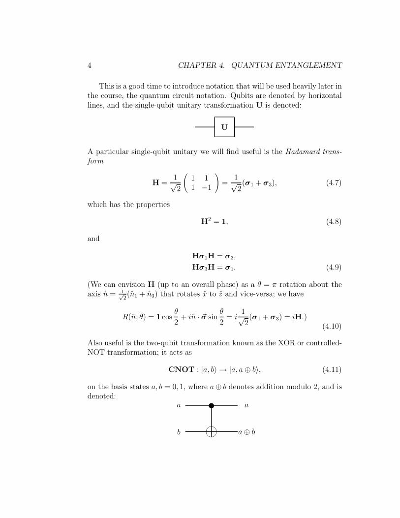
This is a good time to introduce notation that will be used heavily later inthe course, the quantum circuit notation. Qubits are denoted by horizontallines, and the single-qubit unitary transformation U is denoted:

U

A particular single-qubit unitary we will find useful is the Hadamard trans-form

H =1√2

(

1 11 −1

)

=1√2(σ1 + σ3), (4.7)

which has the properties

H2 = 1, (4.8)

and

Hσ1H = σ3,

Hσ3H = σ1. (4.9)

(We can envision H (up to an overall phase) as a θ = π rotation about theaxis n = 1√

2(n1 + n3) that rotates x to z and vice-versa; we have

R(n, θ) = 1 cosθ

2+ in · ~σ sin

θ

2= i

1√2(σ1 + σ3) = iH.)

(4.10)

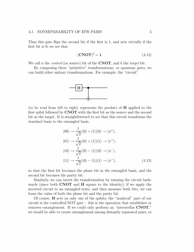
Also useful is the two-qubit transformation known as the XOR or controlled-NOT transformation; it acts as

CNOT : |a, b〉 → |a, a⊕ b〉, (4.11)

on the basis states a, b = 0, 1, where a⊕ b denotes addition modulo 2, and isdenoted:

a

b

w

� ��

a⊕ b

a


Thus this gate flips the second bit if the first is 1, and acts trivially if thefirst bit is 0; we see that

(CNOT)2 = 1. (4.12)

We call a the control (or source) bit of the CNOT, and b the target bit.By composing these “primitive” transformations, or quantum gates, we

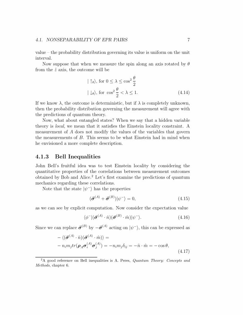
can build other unitary transformations. For example, the “circuit”

H u

i

(to be read from left to right) represents the product of H applied to thefirst qubit followed by CNOT with the first bit as the source and the secondbit as the target. It is straightforward to see that this circuit transforms thestandard basis to the entangled basis,

|00〉 → 1√2(|0〉 + |1〉)|0〉 → |φ+〉,

|01〉 → 1√2(|0〉 + |1〉)|1〉 → |ψ+〉,

|10〉 → 1√2(|0〉 − |1〉)|0〉 → |φ−〉,

|11〉 → 1√2(|0〉 − |1〉)|1〉 → |ψ−〉, (4.13)

so that the first bit becomes the phase bit in the entangled basis, and thesecond bit becomes the parity bit.

Similarly, we can invert the transformation by running the circuit back-wards (since both CNOT and H square to the identity); if we apply theinverted circuit to an entangled state, and then measure both bits, we canlearn the value of both the phase bit and the parity bit.

Of course, H acts on only one of the qubits; the “nonlocal” part of ourcircuit is the controlled-NOT gate – this is the operation that establishes orremoves entanglement. If we could only perform an “interstellar CNOT,”we would be able to create entanglement among distantly separated pairs, or


extract the information encoded in entanglement. But we can’t. To do itsjob, the CNOT gate must act on its target without revealing the value ofits source. Local operations and classical communication will not suffice.

4.1.2 Einstein locality and hidden variables

Einstein was disturbed by quantum entanglement. Eventually, he along withPodolsky and Rosen sharpened their discomfort into what they regarded asa paradox. As later reinterpreted by Bohm, the situation they described isreally the same as that discussed in §2.5.3. Given a maximally entangledstate of two qubits shared by Alice and Bob, Alice can choose one of severalpossible measurements to perform on her spin that will realize different pos-sible ensemble interpretations of Bob’s density matrix; for example, she canprepare either σ1 or σ3 eigenstates.

We have seen that Alice and Bob are unable to exploit this phenomenonfor faster-than-light communication. Einstein knew this but he was stilldissatisfied. He felt that in order to be considered a complete descriptionof physical reality a theory should meet a stronger criterion, that might becalled Einstein locality:

Suppose that A and B are spacelike separated systems. Then ina complete description of physical reality an action performed onsystem A must not modify the description of system B.

But if A and B are entangled, a measurement of A is performed and aparticular outcome is known to have been obtained, then the density matrixof B does change. Therefore, by Einstein’s criterion, the description of aquantum system by a wavefunction cannot be considered complete.

Einstein seemed to envision a more complete description that would re-move the indeterminacy of quantum mechanics. A class of theories with thisfeature are called local hidden-variable theories. In a hidden variable the-ory, measurement is actually fundamentally deterministic, but appears to beprobabilistic because some degrees of freedom are not precisely known. Forexample, perhaps when a spin is prepared in what quantum theory woulddescribe as the pure state | ↑z〉, there is actually a deeper theory in whichthe state prepared is parametrized as (z, λ) where λ (0 ≤ λ ≤ 1) is thehidden variable. Suppose that with present-day experimental technique, wehave no control over λ, so when we prepare the spin state, λ might take any


value – the probability distribution governing its value is uniform on the unitinterval.

Now suppose that when we measure the spin along an axis rotated by θfrom the z axis, the outcome will be

| ↑θ〉, for 0 ≤ λ ≤ cos2 θ

2

| ↓θ〉, for cos2 θ

2< λ ≤ 1. (4.14)

If we know λ, the outcome is deterministic, but if λ is completely unknown,then the probability distribution governing the measurement will agree withthe predictions of quantum theory.

Now, what about entangled states? When we say that a hidden variabletheory is local, we mean that it satisfies the Einstein locality constraint. Ameasurement of A does not modify the values of the variables that governthe measurements of B. This seems to be what Einstein had in mind whenhe envisioned a more complete description.

4.1.3 Bell Inequalities

John Bell’s fruitful idea was to test Einstein locality by considering thequantitative properties of the correlations between measurement outcomesobtained by Bob and Alice.2 Let’s first examine the predictions of quantummechanics regarding these correlations.

Note that the state |ψ−〉 has the properties

(~σ(A) + ~σ(B))|ψ−〉 = 0, (4.15)

as we can see by explicit computation. Now consider the expectation value

〈φ−|(~σ(A) · n)(~σ(B) · m)|ψ−〉. (4.16)

Since we can replace ~σ(B) by −~σ(A) acting on |ψ−〉, this can be expressed as

− 〈(~σ(A) · n)(~σ(A) · m)〉 =

− nimjtr(ρAσ(A)i σ

(A)j ) = −nimjδij = −n · m = − cos θ,

(4.17)

2A good reference on Bell inequalities is A. Peres, Quantum Theory: Concepts and

Methods, chapter 6.


where θ is the angle between the axes n and m. Thus we find that themeasurement outcomes are always perfectly anticorrelated when we measureboth spins along the same axis n, and we have also obtained a more generalresult that applies when the two axes are different. Since the projectionoperator onto the spin up (spin down) states along n is E(n,±) = 1

2(1±n·~σ),

we also obtain

〈ψ−|E(A)(n,+)E(B)(m,+)|ψ−〉

= 〈ψ−|E(A)(n,−)E(B)(m,−)|ψ−〉 =1

4(1 − cos θ),

〈ψ−|E(A)(n,+)E(B)(m,−)|ψ−〉

= 〈ψ−|E(A)(n,−)E(B)(m,+)|ψ−〉 =1

4(1 + cos θ); (4.18)

The probability that the outcomes are opposite is 12(1+cos θ), and the prob-

ability that the outcomes are the same is 12(1 − cos θ).

Now suppose Alice will measure her spin along one of the three axes inthe x− z plane,

n1 = (0, 0, 1)

n2 =

(√3

2, 0,−1

2

)

n3 =

(

−√

3

2, 0,−1

2

)

. (4.19)

Once she performs the measurement, she disturbs the state of the spin, soshe won’t have a chance to find out what would have happened if she hadmeasured along a different axis. Or will she? If she shares the state |ψ−〉with Bob, then Bob can help her. If Bob measures along, say, n2, and sendsthe result to Alice, then Alice knows what would have happened if she hadmeasured along n2, since the results are perfectly anticorrelated. Now she cango ahead and measure along n1 as well. According to quantum mechanics,the probability that measuring along n1, and n2 give the same result is

Psame =1

2(1 − cos θ) =

1

4. (4.20)

(We have cos θ = 1/2 because Bob measures along −n2 to obtain Alice’sresult for measuring along n2). In the same way, Alice and Bob can work


together to determine outcomes for the measurement of Alice’s spin alongany two of the axes n1, n2, and n3.

It is as though three coins are resting on a table; each coin has either theheads (H) or tails (T) side facing up, but the coins are covered, at first, sowe don’t know which. It is possible to reveal two of the coins (measure thespin along two of the axes) to see if they are H or T , but then the third coinalways disappears before we get a chance to uncover it (we can’t measure thespin along the third axis).

Now suppose that there are actually local hidden variables that providea complete description of this system, and the quantum correlations are toarise from a probability distribution governing the hidden variables. Then,in this context, the Bell inequality is the statement

Psame(1, 2) + Psame(1, 3) + Psame(2, 3) ≥ 1, (4.21)

where Psame(i, j) denotes the probability that coins i and j have the samevalue (HH or TT ). This is satisfied by any probability distribution for thethree coins because no matter what the values of the coins, there will alwaysbe two that are the same. But in quantum mechanics,

Psame(1, 2) + Psame(1, 3) + Psame(2, 3) = 3 · 1

4=

3

4< 1.

(4.22)

We have found that the correlations predicted by quantum theory are incom-patible with the local hidden variable hypothesis.

What are the implications? To some people, the peculiar correlationsunmasked by Bell’s theorem call out for a deeper explanation than quantummechanics seems to provide. They see the EPR phenomenon as a harbingerof new physics awaiting discovery. But they may be wrong. We have beenwaiting over 60 years since EPR, and so far no new physics.

Perhaps we have learned that it can be dangerous to reason about whatmight have happened, but didn’t actually happen. (Of course, we do thisall the time in our everyday lives, and we usually get away with it, butsometimes it gets us into trouble.) I claimed that Alice knew what wouldhappen when she measured along n2, because Bob measured along n2, andevery time we have ever checked, their measurement outcomes are alwaysperfectly anticorrelated. But Alice did not measure along n2; she measuredalong n1 instead. We got into trouble by trying to assign probabilities to theoutcomes of measurements along n1, n2, and n3, even though we can only


perform one of those measurements. This turned out to lead to mathematicalinconsistencies, so we had better not do it. From this viewpoint we haveaffirmed Bohr’s principle of complementary — we are forbidden to considersimultaneously the possible outcomes of two mutually exclusive experiments.

Another common attitude is that the violations of the Bell inequalities(confirmed experimentally) have exposed an essential nonlocality built intothe quantum description of Nature. One who espouses this view has implic-itly rejected the complementarity principle. If we do insist on talking aboutoutcomes of mutually exclusive experiments then we are forced to concludethat Alice’s choice of measurement actually exerted a subtle influence on theoutcome of Bob’s measurement. This is what is meant by the “nonlocality”of quantum theory.

By ruling out local hidden variables, Bell demolished Einstein’s dreamthat the indeterminacy of quantum theory could be eradicated by adoptinga more complete, yet still local, description of Nature. If we accept localityas an inviolable principle, then we are forced to accept randomness as anunavoidable and intrinsic feature of quantum measurement, rather than aconsequence of incomplete knowledge.

The human mind seems to be poorly equipped to grasp the correlationsexhibited by entangled quantum states, and so we speak of the weirdnessof quantum theory. But whatever your attitude, experiment forces you toaccept the existence of the weird correlations among the measurement out-comes. There is no big mystery about how the correlations were established– we saw that it was necessary for Alice and Bob to get together at somepoint to create entanglement among their qubits. The novelty is that, evenwhen A and B are distantly separated, we cannot accurately regard A andB as two separate qubits, and use classical information to characterize howthey are correlated. They are more than just correlated, they are a singleinseparable entity. They are entangled.

4.1.4 Photons

Experiments that test the Bell inequality are done with entangled photons,not with spin−1

2objects. What are the quantum-mechanical predictions for

photons?Suppose, for example, that an excited atom emits two photons that come

out back to back, with vanishing angular momentum and even parity. If |x〉and |y〉 are horizontal and vertical linear polarization states of the photon,


then we have seen that

|+〉 =1√2(|x〉 + i|y〉),

|−〉 =1√2(i|x〉+ |y〉), (4.23)

are the eigenstates of helicity (angular momentum along the axis of propaga-tion z. For two photons, one propagating in the +z direction, and the otherin the −z direction, the states

|+〉A|−〉B|−〉A|+〉B (4.24)

are invariant under rotations about z. (The photons have opposite values ofJz, but the same helicity, since they are propagating in opposite directions.)Under a reflection in the y − z plane, the polarization states are modifiedaccording to

|x〉 → −|x〉, |+〉 → +i|−〉,|y〉 → |y〉, |−〉 → −i|+〉; (4.25)

therefore, the parity eigenstates are entangled states

1√2(|+〉A|−〉B ± |−〉A|+〉B). (4.26)

The state with Jz = 0 and even parity, then, expressed in terms of the linearpolarization states, is

− i√2(|+〉A|−〉B + |−〉A|+〉B)

=1√2(|xx〉AB + |yy〉AB)n = |φ+〉AB . (4.27)

Because of invariance under rotations about z, the state has this form irre-spective of how we orient the x and y axes.

We can use a polarization analyzer to measure the linear polarization ofeither photon along any axis in the xy plane. Let |x(θ)〉 and |y(θ)〉 denote


the linear polarization eigenstates along axes rotated by angle θ relative tothe canonical x and y axes. We may define an operator (the analog of ~σ · n)

τ (θ) = |x(θ)〉〈x(θ)| − |y(θ)〉〈y(θ)|, (4.28)

which has these polarization states as eigenstates with respective eigenvalues±1. Since

|x(θ)〉 =

(

cos θsin θ

)

, |y(θ)〉 =

(

− sin θcos θ

)

, (4.29)

in the |x〉, |y〉 basis, we can easily compute the expectation value

AB〈φ+|τ (A)(θ1)τ(B)(θ2)|φ+〉AB . (4.30)

Using rotational invariance:

= AB〈φ+|τ (A)(0)τ (B)(θ2 − θ1)|φ+〉AB

=1

2B〈x|τ (B)(θ2 − θ1)|x〉B − 1

2B〈y|τ (B)(θ2 − θ1)|y〉B

= cos2(θ2 − θ1) − sin2(θ2 − θ1) = cos[2(θ2 − θ1)]. (4.31)

(For spin-12

objects, we would obtain

AB〈φ+|(~σ(A) · n1)(~σ(B) · n2) = n1 · n2 = cos(θ2 − θ1); (4.32)

the argument of the cosine is different than in the case of photons, becausethe half angle θ/2 appears in the formula analogous to eq. (4.29).)

4.1.5 More Bell inequalities

So far, we have considered only one (particularly interesting) case of the Bellinequality. Here we will generalize the result.

Consider a correlated pair of photons, A and B. We may choose tomeasure the polarization of photon A along either one of two axes, α or α′.The corresponding observables are denoted

a = τ (A)(α)

a′ = τ (A)(α′). (4.33)


Similarly, we may choose to measure photon B along either axis β or axis β ′;the corresponding observables are

b = τ (B)(β)

b = τ (B)(β ′). (4.34)

We will, to begin with, consider the special case α′ = β ′ ≡ γ.Now, if we make the local hidden variable hypothesis, what can be in-

fer about the correlations among these observables? We’ll assume that theprediction of quantum mechanics is satisfied if we measure a′ and b′, namely

〈a′b′〉 = 〈τ (B)(γ)τ (B)(γ)〉 = 1; (4.35)

when we measure both photons along the same axes, the outcomes alwaysagree. Therefore, these two observables have exactly the same functionaldependence on the hidden variables – they are really the same observable,with we will denote c.

Now, let a, b, and c be any three observables with the properties

a, b, c = ±1; (4.36)

i.e., they are functions of the hidden variables that take only the two values±1. These functions satisfy the identity

a(b − c) = ab(1 − bc). (4.37)

(We can easily verify the identity by considering the cases b − c = 0, 2,−2.)Now we take expectation values by integrating over the hidden variables,weighted by a nonnegative probability distribution:

〈ab〉 − 〈ac〉 = 〈ab(1 − bc)〉. (4.38)

Furthermore, since ab = ±1, and 1 − bc is nonnegative, we have

|〈ab(1 − bc)〉|≤ |〈1 − bc〉| = 1 − 〈bc〉. (4.39)

We conclude that

|〈ab〉 − 〈ac〉| ≤ 1 − 〈bc〉. (4.40)


This is the Bell inequality.To make contact with our earlier discussion, consider a pair of spin-1

2

objects in the state |φ+〉, where α, β, γ are separated by successive 60o angles.Then quantum mechanics predicts

〈ab〉 =1

2

〈bc〉 =1

2

〈ac〉 = −1

2, (4.41)

which violates the Bell inequality:

1 =1

2+

1

26≤ 1 − 1

2=

1

2. (4.42)

For photons, to obtain the same violation, we halve the angles, so α, β, γ areseparated by 30o angles.

Return now to the more general case α′ 6= β ′. We readily see thata,a′, b, b′ = ±1 implies that

(a + a′)b − (a − a′)b′ = ±2, (4.43)

(by considering the two cases a + a′ = 0 and a − a′ = 0), or

〈ab〉 + 〈a′b〉 + 〈a′b′〉 − 〈ab′〉 = 〈θ〉, (4.44)

where θ = ±2. Evidently

|〈θ〉| ≤ 2, (4.45)

so that

|〈ab〉 + 〈a′b〉 + 〈a′b′〉 − 〈ab′〉| ≤ 2. (4.46)

This result is called the CHSH (Clauser-Horne-Shimony-Holt) inequality. Tosee that quantum mechanics violates it, consider the case for photons whereα, β, α′, β ′ are separated by successive 22.5◦ angles, so that the quantum-mechanical predictions are

〈ab〉 = 〈a′b〉 = 〈a′b′〉 = cosπ

4=

1√2,

〈ab′〉 = cos3π

4= − 1√

2, (4.47)


while

2√

2 6≤ 2. (4.48)

4.1.6 Maximal violation

We can see that the case just considered (α, β, α′, β ′ separated by successive22.5o angles) provides the largest possible quantum mechanical violation ofthe CHSH inequality. In quantum theory, suppose that a,a′, b, b′ are ob-servables that satisfy

a2 = a′2 = b2 = b′2 = 1, (4.49)

and

0 = [a, b] = [a, b′] = [a′, b] = [a′, b′]. (4.50)

Let

C = ab + a′b + a′b′ − ab′. (4.51)

Then

C2 = 4 + aba′b′ − a′bab′ + a′b′ab − ab′a′b. (4.52)

(You can check that the other terms cancel)

= 4 + [a,a′][b, b′]. (4.53)

The sup norm ‖ M ‖ of a bounded operator M is defined by

‖ M ‖= sup

|ψ〉

(

‖ M|ψ〉 ‖‖ |ψ〉 ‖

)

; (4.54)

it is easy to verify that the sup norm has the properties

‖ MN ‖ ≤‖ M ‖‖ N ‖,‖ M + N ‖ ≤‖ M ‖ + ‖ N ‖, (4.55)

and therefore

‖ [M,N] ‖≤‖ MN ‖ + ‖ NM ‖≤ 2 ‖ M ‖‖ N ‖ . (4.56)


We conclude that

‖ C2 ‖≤ 4 + 4 ‖ a ‖ · ‖ a′ ‖ · ‖ b ‖ · ‖ b′ ‖= 8, (4.57)

or

‖ C ‖≤ 2√

2 (4.58)

(Cirel’son’s inequality). Thus, the expectation value of C cannot exceed2√

2, precisely the value that we found to be attained in the case whereα, β, α′, β ′ are separated by successive 22.5o angles. The violation of theCHSH inequality that we found is the largest violation allowed by quantumtheory.

4.1.7 The Aspect experiment

The CHSH inequality was convincingly tested for the first time by Aspectand collaborators in 1982. Two entangled photons were produced in the de-cay of an excited calcium atom, and each photon was directed by a switchto one of two polarization analyzers, chosen pseudo-randomly. The photonswere detected about 12m apart, corresponding to a light travel time of about40 ns. This time was considerably longer than either the cycle time of theswitch, or the difference in the times of arrival of the two photons. There-fore the “decision” about which observable to measure was made after thephotons were already in flight, and the events that selected the axes for themeasurement of photons A and B were spacelike separated. The results wereconsistent with the quantum predictions, and violated the CHSH inequal-ity by five standard deviations. Since Aspect, many other experiments haveconfirmed this finding.

4.1.8 Nonmaximal entanglement

So far, we have considered the Bell inequality violations predicted by quan-tum theory for a maximally entangled state such as |φ+〉. But what aboutmore general states such as

|φ〉 = α|00〉 + β|11〉? (4.59)

(Any pure state of two qubits can be expressed this way in the Schmidt basis;by adopting suitable phase conventions, we may assume that α and β arereal and nonnegative.)


Consider first the extreme case of separable pure states, for which

〈ab〉 = 〈a〉〈b〉. (4.60)

In this case, it is clear that no Bell inequality violation can occur, becausewe have already seen that a (local) hidden variable theory does exist thatcorrectly reproduces the predictions of quantum theory for a pure state of asingle qubit. Returning to the spin-1

2notation, suppose that we measure the

spin of each particle along an axis n = (sin θ, 0, cos θ) in the xz plane. Then

a = (σ(A) · n1) =

(

cos θ1 sin θ1

sin θ1 − cos θ1

)(A)

,

b = (σ(B) · n2) =

(

cos θ2 sin θ2

sin θ2 − cos θ2

)(B)

, (4.61)

so that quantum mechanics predicts

〈ab〉 = 〈φ|ab|φ〉= cos θ1 cos θ2 + 2αβ sin θ1 sin θ2 (4.62)

(and we recover cos(θ1−θ2) in the maximally entangled case α = β = 1/√

2).Now let us consider, for simplicity, the (nonoptimal!) special case

θA = 0, θ′A =π

2, θ′B = −θB, (4.63)

so that the quantum predictions are:

〈ab〉 = cos θB = 〈ab′〉〈a′b〉 = 2αβ sin θB = −〈a′b′〉 (4.64)

Plugging into the CHSH inequality, we obtain

| cos θB − 2αβ sin θB| ≤ 1, (4.65)

and we easily see that violations occur for θB close to 0 or π. Expanding tolinear order in θB, the left hand side is

' 1 − 2αβθB, (4.66)

which surely exceeds 1 for θB negative and small.We have shown, then, that any entangled pure state of two qubits violates

some Bell inequality. It is not hard to generalize the argument to an arbitrarybipartite pure state. For bipartite pure states, then, “entangled” is equivalentto “Bell-inequality violating.” For bipartite mixed states, however, we willsee shortly that the situation is more subtle.


4.2 Uses of Entanglement

After Bell’s work, quantum entanglement became a subject of intensive studyamong those interested in the foundations of quantum theory. But morerecently (starting less than ten years ago), entanglement has come to beviewed not just as a tool for exposing the weirdness of quantum mechanics,but as a potentially valuable resource. By exploiting entangled quantumstates, we can perform tasks that are otherwise difficult or impossible.

4.2.1 Dense coding

Our first example is an application of entanglement to communication. Alicewants to send messages to Bob. She might send classical bits (like dots anddashes in Morse code), but let’s suppose that Alice and Bob are linked bya quantum channel. For example, Alice can prepare qubits (like photons) inany polarization state she pleases, and send them to Bob, who measures thepolarization along the axis of his choice. Is there any advantage to sendingqubits instead of classical bits?

In principle, if their quantum channel has perfect fidelity, and Alice andBob perform the preparation and measurement with perfect efficiency, thenthey are no worse off using qubits instead of classical bits. Alice can prepare,say, either | ↑z〉 or | ↓z〉, and Bob can measure along z to infer the choiceshe made. This way, Alice can send one classical bit with each qubit. Butin fact, that is the best she can do. Sending one qubit at a time, no matterhow she prepares it and no matter how Bob measures it, no more than oneclassical bit can be carried by each qubit. (This statement is a special caseof a bound proved by Kholevo (1973) on the classical information capacityof a quantum channel.)

But now, let’s change the rules a bit – let’s suppose that Alice and Bobshare an entangled pair of qubits in the state |φ+〉AB . The pair was preparedlast year; one qubit was shipped to Alice and the other to Bob, anticipatingthat the shared entanglement would come in handy someday. Now, use ofthe quantum channel is very expensive, so Alice can afford to send only onequbit to Bob. Yet it is of the utmost importance for Alice to send Bob twoclassical bits of information.

Fortunately, Alice remembers about the entangled state |φ+〉AB that sheshares with Bob, and she carries out a protocol that she and Bob had ar-ranged for just such an emergency. On her member of the entangled pair,

4.2. USES OF ENTANGLEMENT 19

she can perform one of four possible unitary transformations:

1) 1 (she does nothing),

2) σ1 (180o rotation about x-axis),

3) σ2 (180o rotation about y-axis),

4) σ3 (180o rotation about z-axis).

As we have seen, by doing so, she transforms |φ+〉AB to one of 4 mutuallyorthogonal states:

1) |φ+〉AB ,

2) |ψ+〉AB ,

3) |ψ−〉AB ,

4) |φ−〉AB .

Now, she sends her qubit to Bob, who receives it and then performs an or-thogonal collective measurement on the pair that projects onto the maximallyentangled basis. The measurement outcome unambiguously distinguishes thefour possible actions that Alice could have performed. Therefore the singlequbit sent from Alice to Bob has successfully carried 2 bits of classical infor-mation! Hence this procedure is called “dense coding.”

A nice feature of this protocol is that, if the message is highly confidential,Alice need not worry that an eavesdropper will intercept the transmittedqubit and decipher her message. The transmitted qubit has density matrixρA = 1

21A, and so carries no information at all. All the information is in

the correlations between qubits A and B, and this information is inaccessibleunless the adversary is able to obtain both members of the entangled pair.(Of course, the adversary can “jam” the channel, preventing the informationbut reaching Bob.)

From one point of view, Alice and Bob really did need to use the channeltwice to exchange two bits of information – a qubit had to be transmitted forthem to establish their entangled pair in the first place. (In effect, Alice hasmerely sent to Bob two qubits chosen to be in one of the four mutually or-thogonal entangled states.) But the first transmission could have taken placea long time ago. The point is that when an emergency arose and two bits


had to be sent immediately while only one use of the channel was possible,Alice and Bob could exploit the pre-existing entanglement to communicatemore efficiently. They used entanglement as a resource.

4.2.2 EPR Quantum Key Distribution

Everyone has secrets, including Alice and Bob. Alice needs to send a highlyprivate message to Bob, but Alice and Bob have a very nosy friend, Eve, whothey know will try to listen in. Can they communicate with assurance thatEve is unable to eavesdrop?

Obviously, they should use some kind of code. Trouble is, aside frombeing very nosy, Eve is also very smart. Alice and Bob are not confidentthat they are clever enough to devise a code that Eve cannot break.

Except there is one coding scheme that is surely unbreakable. If Aliceand Bob share a private key, a string of random bits known only to them,then Alice can convert her message to ASCII (a string of bits no longer thanthe key) add each bit of her message (module 2) to the corresponding bit ofthe key, and send the result to Bob. Receiving this string, Bob adds the keyto it to extract Alice’s message.

This scheme is secure because even if Eve should intercept the transmis-sion, she will not learn anything because the transmitted string itself carriesno information – the message is encoded in a correlation between the trans-mitted string and the key (which Eve doesn’t know).

There is still a problem, though, because Alice and Bob need to establisha shared random key, and they must ensure that Eve can’t know the key.They could meet to exchange the key, but that might be impractical. Theycould entrust a third party to transport the key, but what if the intermediaryis secretly in cahoots with Eve? They could use “public key” distributionprotocols, but these are not guaranteed to be secure.

Can Alice and Bob exploit quantum information (and specifically entan-glement) to solve the key exchange problem? They can! This observationis the basis of what is sometimes called “quantum cryptography.” But sincequantum mechanics is really used for key exchange rather than for encoding,it is more properly called “quantum key distribution.”

Let’s suppose that Alice and Bob share a supply of entangled pairs, eachprepared in the state |ψ−〉. To establish a shared private key, they may carryout this protocol.


For each qubit in her/his possession, Alice and Bob decide to measureeither σ1 or σ3. The decision is pseudo-random, each choice occuring withprobability 1/2. Then, after the measurements are performed, both Aliceand Bob publicly announce what observables they measured, but do notreveal the outcomes they obtained. For those cases (about half) in whichthey measured their qubits along different axes, their results are discarded(as Alice and Bob obtained uncorrelated outcomes). For those cases in whichthey measured along the same axis, their results, though random, are perfectly(anti-)correlated. Hence, they have established a shared random key.

But, is this protocol really invulnerable to a sneaky attack by Eve? Inparticular, Eve might have clandestinely tampered with the pairs at sometime and in the past. Then the pairs that Alice and Bob possess might be(unbeknownst to Alice and Bob) not perfect |ψ−〉’s, but rather pairs that areentangled with qubits in Eve’s possession. Eve can then wait until Alice andBob make their public announcements, and proceed to measure her qubitsin a manner designed to acquire maximal information about the results thatAlice and Bob obtained. Alice and Bob must protect themselves against thistype of attack.

If Eve has indeed tampered with Alice’s and Bob’s pairs, then the mostgeneral possible state for an AB pair and a set of E qubits has the form

|Υ〉ABE = |00〉AB |e00〉E + |01〉AB |e01〉E+ |10〉AB |e10〉E + |11〉AB |e11〉E . (4.67)

But now recall that the defining property or |ψ−〉 is that it is an eigenstate

with eigenvalue −1 of both σ(A)1 σ

(B)1 and σ

(A)3 σ

(B)3 . Suppose that A and B

are able to verify that the pairs in their possession have this property. Tosatisfy σ

(A)3 σ

(B)3 = −1, we must have

|Υ〉AB = |01〉AB |e01〉E + |10〉AB |e10〉E , (4.68)

and to also satisfy σ(A)1 σ

(B)1 = −1, we must have

|Υ〉ABE =1√2(|01〉 − |10〉)|e〉E = |ψ−〉|e〉. (4.69)

We see that it is possible for the AB pairs to be eigenstates of σ(A)1 σ

(B)1

and σ(A)3 σ

(B)3 only if they are completely unentangled with Eve’s qubits.


Therefore, Eve will not be able to learn anything about Alice’s and Bob’smeasurement results by measuring her qubits. The random key is secure.

To verify the properties σ(A)1 σ

(B)1 = −1 = σ

(A)3 σ

(B)3 , Alice and Bob can

sacrifice a portion of their shared key, and publicly compare their measure-ment outcomes. They should find that their results are indeed perfectlycorrelated. If so they will have high statistical confidence that Eve is unableto intercept the key. If not, they have detected Eve’s nefarious activity. Theymay then discard the key, and make a fresh attempt to establish a securekey.

As I have just presented it, the quantum key distribution protocol seemsto require entangled pairs shared by Alice and Bob, but this is not reallyso. We might imagine that Alice prepares the |ψ−〉 pairs herself, and thenmeasures one qubit in each pair before sending the other to Bob. This iscompletely equivalent to a scheme in which Alice prepares one of the fourstates

| ↑z〉, | ↓z〉, | ↑x〉, | ↓x〉, (4.70)

(chosen at random, each occuring with probability 1/4) and sends the qubitto Bob. Bob’s measurement and the verification are then carried out asbefore. This scheme (known as BB84 in quantum key distribution jargon) isjust as secure as the entanglement-based scheme.3

Another intriguing variation is called the “time-reversed EPR” scheme.Here both Alice and Bob prepare one of the four states in eq. (4.70), andthey both send their qubits to Charlie. Then Charlie performs a Bell mea-surement on the pair, orthogonally projecting out one of |φ±〉|ψ±〉, and hepublicly announces the result. Since all four of these states are simultaneouseigenstates of σ

(A)1 σ

(B)1 and σ

(A)3 σ

(B)3 , when Alice and Bob both prepared

their spins along the same axis (as they do about half the time) they sharea single bit.4 Of course, Charlie could be allied with Eve, but Alice and Bobcan verify that Charlie has acquired no information as before, by compar-ing a portion of their key. This scheme has the advantage that Charlie could

3Except that in the EPR scheme, Alice and Bob can wait until just before they need totalk to generate the key, thus reducing the risk that Eve might at some point burglarizeAlice’s safe to learn what states Alice prepared (and so infer the key).

4Until Charlie does his measurement, the states prepared by Bob and Alice are to-tally uncorrelated. A definite correlation (or anti-correlation) is established after Charlieperforms his measurement.


operate a central switching station by storing qubits received from many par-ties, and then perform his Bell measurement when two of the parties requesta secure communication link. A secure key can be established even if thequantum communication line is down temporarily, as long as both partieshad the foresight to send their qubits to Charlie on an earlier occasion (whenthe quantum channel was open.)

So far, we have made the unrealistic assumption that the quantum com-munication channel is perfect, but of course in the real world errors willoccur. Therefore even if Eve has been up to no mischief, Alice and Bobwill sometimes find that their verification test will fail. But how are they todistinguish errors due to imperfections of the channel from errors that occurbecause Eve has been eavesdropping?

To address this problem, Alice and Bob must enhance their protocol intwo ways. First they must implement (classical) error correction to reducethe effective error rate. For example, to establish each bit of their sharedkey they could actually exchange a block of three random bits. If the threebits are not all the same, Alice can inform Bob which of the three is differentthan the other two; Bob can flip that bit in his block, and then use majorityvoting to determine a bit value for the block. This way, Alice and Bob sharethe same key bit even if an error occured for one bit in the block of three.

However, error correction alone does not suffice to ensure that Eve hasacquired negligible information about the key – error correction must besupplemented by (classical) privacy amplification. For example, after per-forming error correction so that they are confident that they share the samekey, Alice and Bob might extract a bit of “superkey” as the parity of n keybits. To know anything about the parity of n bits, Eve would need to knowsomething about each of the bits. Therefore, the parity bit is considerablymore secure, on the average, than each of the individual key bits.

If the error rate of the channel is low enough, one can hope to show thatquantum key distribution, supplemented by error correction and privacy am-plification, is invulnerable to any attack that Eve might muster (in the sensethat the information acquired by Eve can be guaranteed to be arbitrarilysmall). Whether this has been established is, at the moment, a matter ofcontroversy.


4.2.3 No cloning

The security of quantum key distribution is based on an essential differencebetween quantum information and classical information. It is not possibleto acquire information that distinguishes between nonorthogonal quantumstates without disturbing the states.

For example, in the BB84 protocol, Alice sends to Bob any one of the fourstates | ↑z〉| ↓z〉| ↑x〉| ↓x〉, and Alice and Bob are able to verify that none oftheir states are perturbed by Eve’s attempt at eavesdropping. Suppose, moregenerally, that |ϕ〉 and |ψ〉 are two nonorthogonal states in H (〈ψ|ϕ〉 6= 0)and that a unitary transformation U is applied to H ⊗HE (where HE is aHilbert space accessible to Eve) that leaves both |ψ〉 and |ϕ〉 undisturbed.Then

U : |ψ〉 ⊗ |0〉E → |ψ〉 ⊗ |e〉E ,|ϕ〉 ⊗ |0〉E → |ϕ〉 ⊗ |f〉E , (4.71)

and unitarity implies that

〈ψ|φ〉 = (E〈0| ⊗ 〈ψ|)(|ϕ〉 ⊗ |0〉E)

= (E〈e| ⊗ 〈ψ|)(|ϕ〉 ⊗ |f〉E)

= 〈ψ|ϕ〉E〈e|f〉E . (4.72)

Hence, for 〈ψ|ϕ〉 6= 0, we have E〈e|f〉E = 1, and therefore since the statesare normalized, |e〉 = |f〉. This means that no measurement in HE canreveal any information that distinguishes |ψ〉 from |ϕ〉. In the BB84 casethis argument shows that the state in HE will be the same irrespective ofwhich of the four states | ↑z〉, | ↓z〉, | ↑x〉, | ↓x〉 is sent by Alice, and thereforeEve learns nothing about the key shared by Alice and Bob. On the otherhand, if Alice is sending to Bob one of the two orthogonal states | ↑z〉 or | ↓z〉,there is nothing to prevent Eve from acquiring a copy of the information (aswith classical bits).

We have noted earlier that if we have many identical copies of a qubit,then it is possible to measure the mean value of noncommuting observableslike σ1,σ2, and σ3 to completely determine the density matrix of the qubit.Inherent in the conclusion that nonorthogonal state cannot be distinguishedwithout disturbing them, then, is the implicit provision that it is not possibleto make a perfect copy of a qubit. (If we could, we would make as many copiesas we need to find 〈σ1〉, 〈σ2〉, and 〈σ3〉 to any specified accuracy.) Let’s now


make this point explicit: there is no such thing as a perfect quantum Xeroxmachine.

Orthogonal quantum states (like classical information) can be reliablycopied. For example, the unitary transformation that acts as

U : |0〉A|0〉B → |0〉A|0〉B|1〉A|0〉B → |1〉A|1〉B , (4.73)

copies the first qubit onto the second if the first qubit is in one of the states|0〉A or |1〉A. But if instead the first qubit is in the state |ψ〉 = a|0〉A + b|1〉A,then

U : (a|0〉A + b|1〉A)|0〉B→ a|0〉A|0〉B + b|1〉A|1〉B. (4.74)

Thus is not the state |ψ〉⊗|ψ〉 (a tensor product of the original and the copy);rather it is something very different – an entangled state of the two qubits.

To consider the most general possible quantum Xerox machine, we allowthe full Hilbert space to be larger than the tensor product of the space of theoriginal and the space of the copy. Then the most general “copying” unitarytransformation acts as

U : |ψ〉A|0〉B |0〉E → |ψ〉A|ψ〉B|e〉E|ϕ〉A|0〉B |0〉E → |ϕ〉A|ϕ〉B|f〉E . (4.75)

Unitarity then implies that

A〈ψ|ϕ〉A = A〈ψ|ϕ〉A B〈ψ|ϕ〉B E〈e|f〉E ; (4.76)

therefore, if 〈ψ|ϕ〉 6= 0, then

1 = 〈ψ|ϕ〉 E〈e|f〉E . (4.77)

Since the states are normalized, we conclude that

|〈ψ|ϕ〉| = 1, (4.78)

so that |ψ〉 and |ϕ〉 actually represent the same ray. No unitary machine canmake a copy of both |ϕ〉 and |ψ〉 if |ϕ〉 and |ψ〉 are distinct, nonorthogonalstates. This result is called the no-cloning theorem.


4.2.4 Quantum teleportation

In dense coding, we saw a case where quantum information could be exploitedto enhance the transmission of classical information. Now let’s address aclosely related issue: Can we use classical information to realize transmissionof quantum information?

Alice has a qubit, but she doesn’t know it’s state. Bob needs this qubitdesperately. But that darn quantum channel is down again! Alice can sendonly classical information to Bob.

She could try measuring ~σ · n, projecting her qubit to either | ↑n〉 or | ↓n〉.She could send the measurement outcome to Bob who could then proceed toprepare the state Alice found. But you showed in a homework exercise thatBob’s qubit will not be a perfect copy of Alice’s; on the average we’ll have

F = |B〈 · |ψ〉A|2 =2

3, (4.79)

Thus is a better fidelity than could have been achieved (F = 12) if Bob had

merely chosen a state at random, but it is not nearly as good as the fidelitythat Bob requires.

But then Alice and Bob recall that they share some entangled pairs; whynot use the entanglement as a resource? They carry out this protocol: Aliceunites the unknown qubit |ψ〉C she wants to send to Bob with her memberof a |φ+〉AB pair that she shares with Bob. On these two qubits she performsBell measurement, projecting onto one of the four states |φ±〉CA, |ψ±〉CA. Shesends her measurement outcome (two bits of classical information) to Bobover the classical channel. Receiving this information, Bob performs one offour operations on his qubit |·〉B:

|φ+〉CA → 1B

|ψ+〉CA → σ(B)1

|ψ−〉CA → σ(B)2

|φ−〉CA → σ(B)3 . (4.80)

This action transforms his qubit (his member of the |φ+〉AB pair that heinitially shared with Alice) into a perfect copy of |ψ〉C ! This magic trick iscalled quantum teleportation.

It is a curious procedure. Initially, Bob’s qubit |·〉B is completely unentan-gled with the unknown qubit |ψ〉C, but Alice’s Bell measurement establishes


a correlation between A and C . The measurement outcome is in fact com-pletely random, as you’ll see in a moment, so Alice (and Bob) actually acquireno information at all about |ψ〉 by making this measurement.

How then does the quantum state manage to travel from Alice to Bob?It is a bit puzzling. On the one hand, we can hardly say that the twoclassical bits that were transmitted carried this information – the bits wererandom. So we are tempted to say that the shared entangled pair made theteleportation possible. But remember that the entangled pair was actuallyprepared last year, long before Alice ever dreamed that she would be sendingthe qubit to Bob ...

We should also note that the teleportation procedure is fully consistentwith the no-cloning theorem. True, a copy of the state |ψ〉 appeared in Bob’shands. But the original |ψ〉C had to be destroyed by Alice’s measurementbefore the copy could be created.

How does it work? We merely note that for |ψ〉 = a|0〉 + b|1〉, we maywrite

|ψ〉C|φ+〉AB = (a|0〉C + b|1〉C)1√2(|00〉AB + |11〉AB)

=1√2(a|000〉CAB + a|011〉CAB + b|100〉CAB + b|111〉CAB )

=1

2a(|φ+〉CA + |φ−〉CA)|0〉B +

1

2a(|ψ+〉CA + |ψ−〉CA)|1〉B

+1

2b(|ψ+〉CA − |ψ−〉CA)|0〉B +

1

2b(|φ+〉CA − |φ−〉CA)|1〉B

=1

2|φ+〉CA(a|0〉B + b|1〉B)

+1

2|ψ+〉CA(a|1〉B + b|0〉B)

+1

2|ψ−〉CA(a|1〉B − b|0〉B)

+1

2|φ−〉CA(a|0〉B − b|1〉B)

=1

2|φ+〉CA|ψ〉B +

1

2|ψ+〉CAσ1|ψ〉B

+1

2|ψ−〉CA(−iσ2)|ψ〉B +

1

2|φ−〉CAσ3|ψ〉B. (4.81)

Thus we see that when we perform the Bell measurement on qubits C and


A, all four outcomes are equally likely, and that the actions prescribed inEq. (4.80) will restore Bob’s qubit to the initial state |ψ〉.

chapter 4 quantum entanglement - caltech theoretical particle

Documents