chapter 4 read this chapter together with unit four in...
TRANSCRIPT
Chapter 4 Read this chapter together with unit four in the study guide
Consumer Choice
Copyright © 2012 Pearson Education. All rights reserved. 4 - 2
Topics
1. Preferences.
2. Utility.
3. Budget Constraint.
4. Constrained Consumer Choice.
5. Behavioral Economics.
Copyright © 2012 Pearson Education. All rights reserved. 4 - 3
Premises of Consumer Behavior
• Individual preferences determine the amount of pleasure people derive from the goods and services they consume.
• Consumers face constraints or limits on their choices.
• Consumers maximize their well-being or pleasure from consumption, subject to the constraints they face.

Copyright © 2012 Pearson Education. All rights reserved. 4 - 4
Your first test ……
Date: 3/3/14 Time: AT 17:15-18.30 Venue: SECTION A
Copyright © 2012 Pearson Education. All rights reserved. 4 - 5
Properties of Consumer Preferences
• Completeness - when facing a choice between any two bundles of goods, a consumer can rank them so that one and only one of the following relationships is true: The consumer prefers the first bundle to the second, prefers the second to the first, or is indifferent between them.

Copyright © 2012 Pearson Education. All rights reserved. 4 - 6
Properties of Consumer Preferences (cont.)
• Transitivity - a consumer’s preferences over bundles is consistent in the sense that, if the consumer weakly prefers Bundle z to Bundle y (likes z at least as much as y) and weakly prefers Bundle y to Bundle x, the consumer also weakly prefers Bundle z to Bundle x.
Copyright © 2012 Pearson Education. All rights reserved. 4 - 7
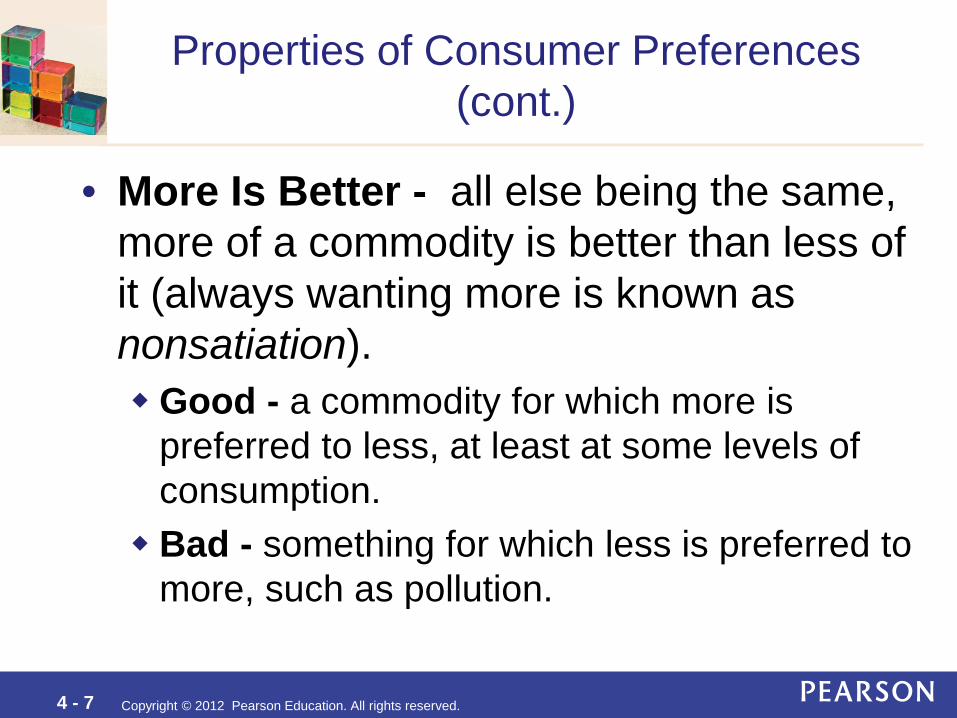
Properties of Consumer Preferences (cont.)
• More Is Better - all else being the same, more of a commodity is better than less of it (always wanting more is known as nonsatiation). Good - a commodity for which more is
preferred to less, at least at some levels of consumption. Bad - something for which less is preferred to
more, such as pollution.
Copyright © 2012 Pearson Education. All rights reserved. 4 - 8
Preference Maps
• Indifference curve - the set of all bundles of goods that a consumer views as being equally desirable. Indifference map - a complete set of
indifference curves that summarize a consumer’s tastes or preferences.
Copyright © 2012 Pearson Education. All rights reserved. 4 - 9
Lisa prefers bundle e to any bundle in area B
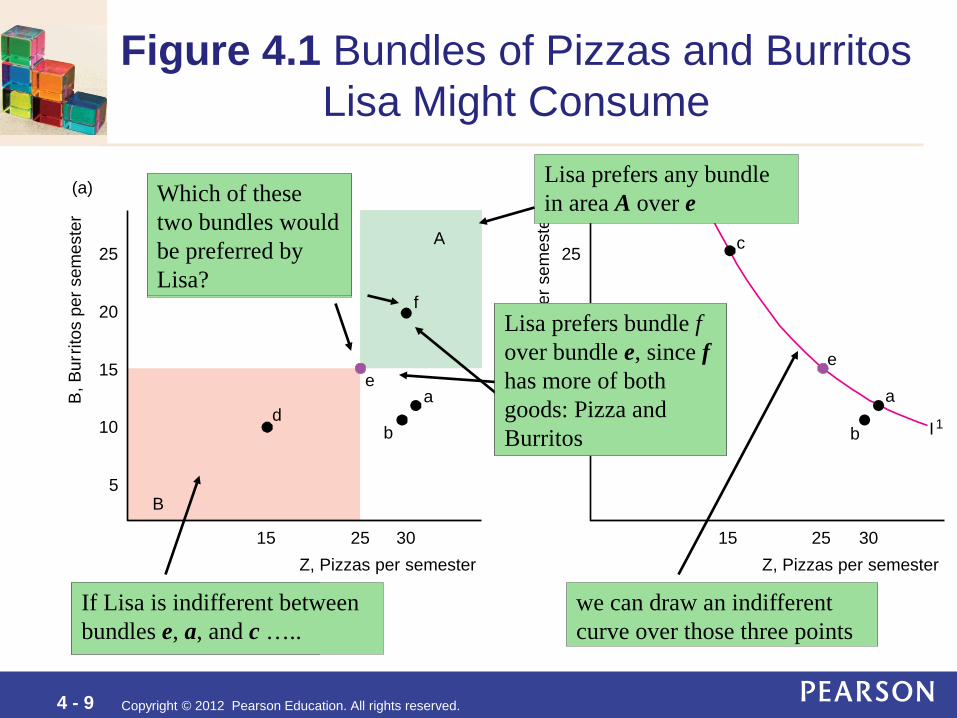
Figure 4.1 Bundles of Pizzas and Burritos Lisa Might Consume
B , B
ur r it
os p
er s
emes
ter
(a)
30 25 15 Z , Pizzas per semester
25
20
15
10
5
d a
b
e
c
f
A
B
B , B
ur r it
os p
er s
emes
ter
(b)
30 25 15 Z , Pizzas per semester
25
20
15
10
a
b I 1
e
c
Which of these two bundles would be preferred by Lisa?
Lisa prefers bundle e over bundle d, since e has more of both goods: Pizza and Burritos
Which of these two bundles would be preferred by Lisa?
Lisa prefers bundle f over bundle e, since f has more of both goods: Pizza and Burritos
Lisa prefers any bundle in area A over e
If Lisa is indifferent between bundles e, a, and c …..
we can draw an indifferent curve over those three points
Copyright © 2012 Pearson Education. All rights reserved. 4 - 10
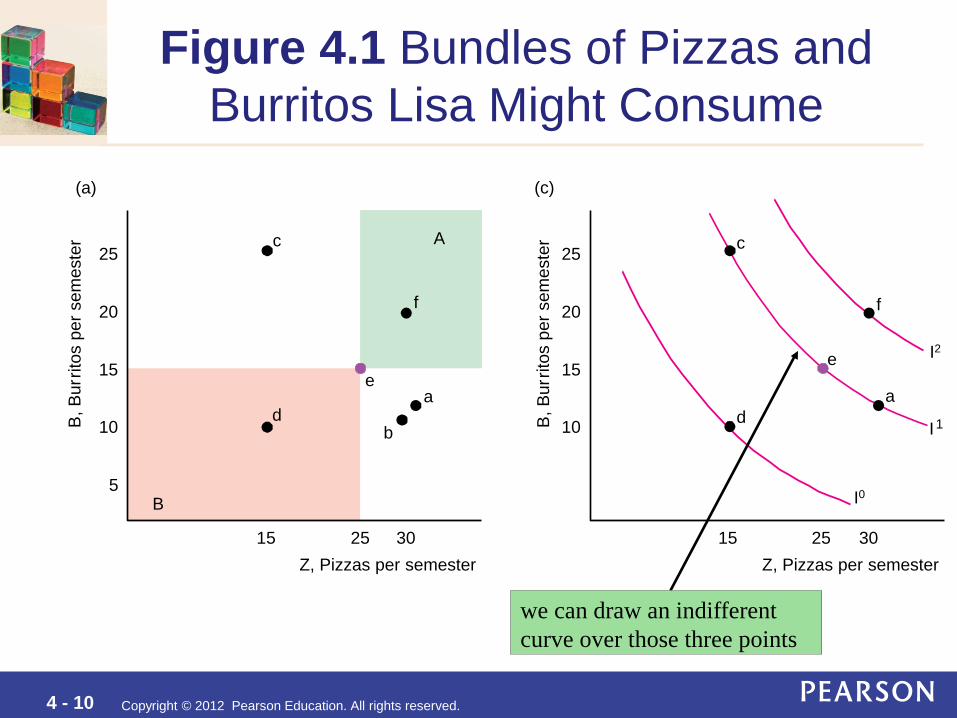
Figure 4.1 Bundles of Pizzas and Burritos Lisa Might Consume
B , B
ur r it
os p
er s
emes
ter
(a)
30 25 15 Z , Pizzas per semester
25
20
15
10
5
d a
b
e
c
f
A
B
B , B
ur r it
os p
er s
emes
ter
(c)
30 25 15 Z , Pizzas per semester
25
20
15
10 d a
I 1
e
c
f
we can draw an indifferent curve over those three points
I2
I0

Copyright © 2012 Pearson Education. All rights reserved. 4 - 11
Properties of Indifference Maps
1. Bundles on indifference curves farther from the origin are preferred to those on indifference curves closer to the origin.
2. There is an indifference curve through every possible bundle.
3. Indifference curves cannot cross. 4. Indifference curves slope downward.
Copyright © 2012 Pearson Education. All rights reserved. 4 - 12
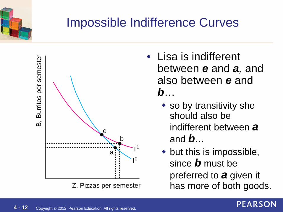
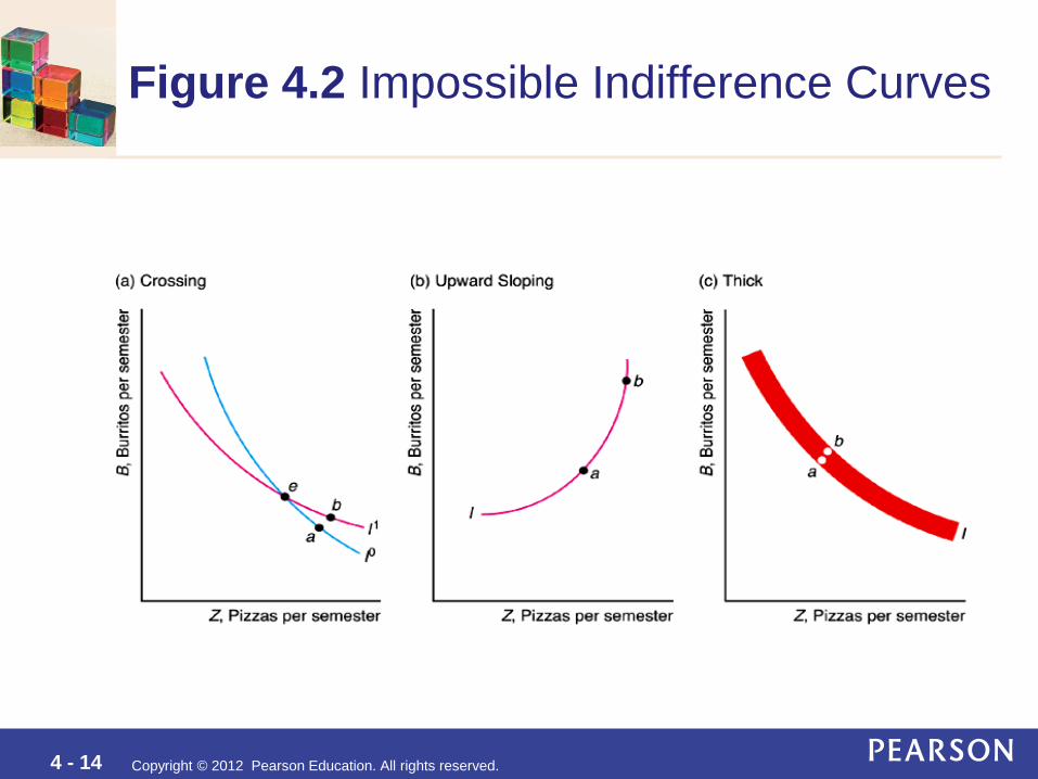
Impossible Indifference Curves
• Lisa is indifferent between e and a, and also between e and b… so by transitivity she
should also be indifferent between a and b…
but this is impossible, since b must be preferred to a given it has more of both goods.
B , B
ur r it
os p
er s
emes
ter
Z , Pizzas per semester
I 1
I 0 a
b e
Copyright © 2012 Pearson Education. All rights reserved. 4 - 13
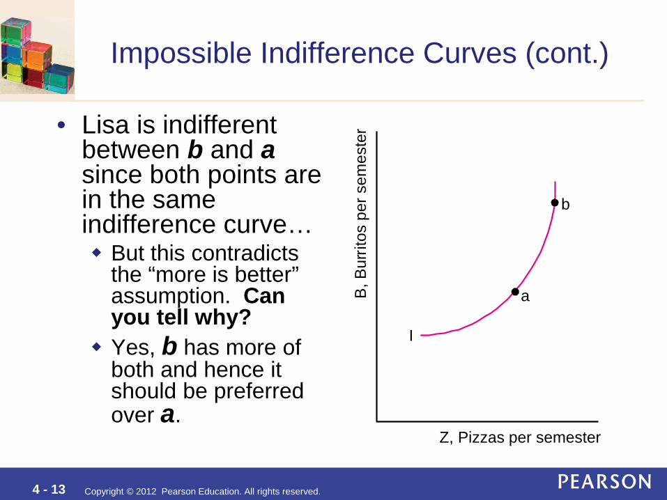
Impossible Indifference Curves (cont.)
• Lisa is indifferent between b and a since both points are in the same indifference curve… But this contradicts
the “more is better” assumption. Can you tell why?
Yes, b has more of both and hence it should be preferred over a.
B , B
ur r it
os p
er s
emes
ter
Z , Pizzas per semester
I
a
b
Copyright © 2012 Pearson Education. All rights reserved. 4 - 14
Figure 4.2 Impossible Indifference Curves

Copyright © 2012 Pearson Education. All rights reserved. 4 - 15
Solved Problem 4.1
• Can indifference curves be thick? • Answer: Draw an indifference curve that is at least two
bundles thick, and show that a preference property is violated

Copyright © 2012 Pearson Education. All rights reserved. 4 - 16
Solved Problem 4.1
• Consumer is indifferent between b and a since both points are in the same indifference curve… But this contradicts the
“more is better” assumption since b has more of both and hence it should be preferred over a.
B , B
ur r it
os p
er s
emes
ter
a
b
Z , Pizzas per semester
I
Copyright © 2012 Pearson Education. All rights reserved. 4 - 17
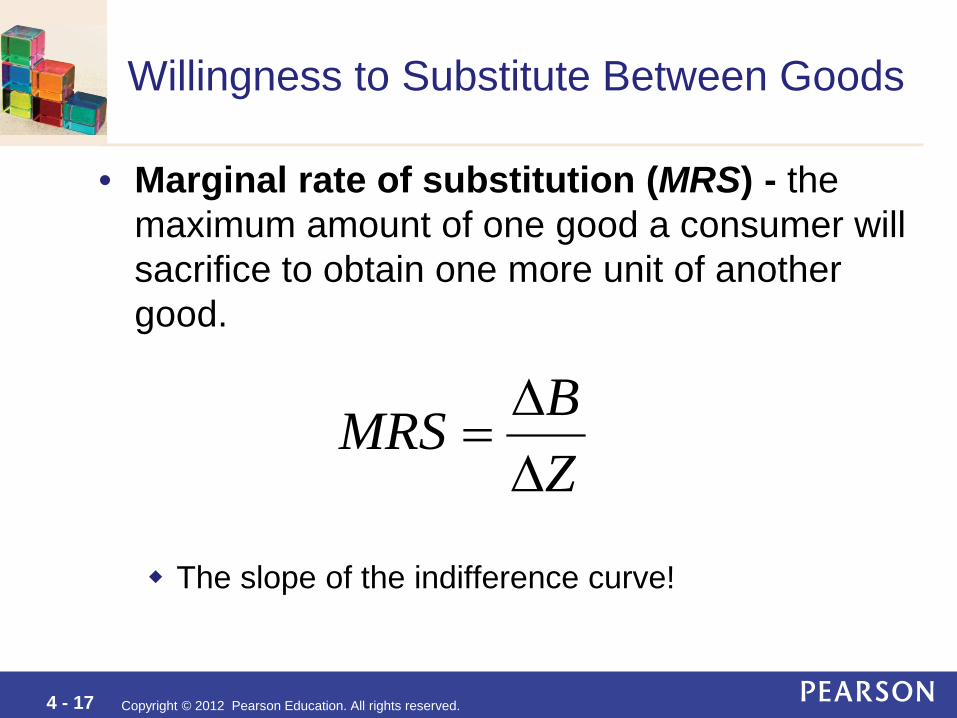
Willingness to Substitute Between Goods
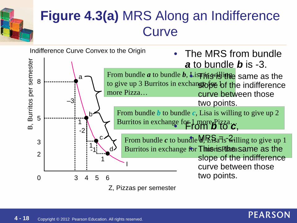
• Marginal rate of substitution (MRS) - the maximum amount of one good a consumer will sacrifice to obtain one more unit of another good. The slope of the indifference curve!
ZBMRS
∆∆
=
Copyright © 2012 Pearson Education. All rights reserved. 4 - 18
From bundle b to bundle c, Lisa is willing to give up 2 Burritos in exchange for 1 more Pizza…
From bundle c to bundle d, Lisa is willing to give up 1 Burritos in exchange for 1 more Pizza…
From bundle a to bundle b, Lisa is willing to give up 3 Burritos in exchange for 1 more Pizza…
Figure 4.3(a) MRS Along an Indifference Curve
B , B
ur r it
os p
er s
emes
ter
Indifference Curve Convex to the Origin
5
3
8
1
-1 1
1 2
0
-2
–3
3 4 5 6 Z , Pizzas per semester
a
b
c
d
I
• The MRS from bundle a to bundle b is -3. This is the same as the
slope of the indifference curve between those two points.
• From b to c, MRS = -2. This is the same as the
slope of the indifference curve between those two points.
Copyright © 2012 Pearson Education. All rights reserved. 4 - 19
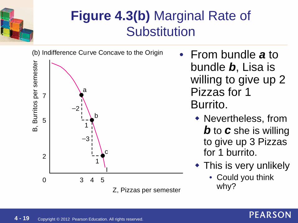
Figure 4.3(b) Marginal Rate of Substitution
• From bundle a to bundle b, Lisa is willing to give up 2 Pizzas for 1 Burrito. Nevertheless, from
b to c she is willing to give up 3 Pizzas for 1 burrito.
This is very unlikely • Could you think
why?
B , B
ur r it
os p
er s
emes
ter
(b) Indif f erence Cu r v e Conc a v e to the O r igin
5
7
1
1
2
0
– 2
– 3
3 4 5 Z , Pizzas per semester
a
b
c
I

Copyright © 2012 Pearson Education. All rights reserved. 4 - 20
Diminishing Marginal Rate of Substitution
• The marginal rate of substitution approaches zero as we move down and to the right along an indifference curve.
• Discussion: could you imagine a good that does not exhibit this property?

Copyright © 2012 Pearson Education. All rights reserved. 4 - 21 Copyright © 2012 Pearson Addison-Wesley. All rights reserved.
Curvature of Indifference Curves
• Casual observation suggests that most people’s indifference curves are convex.
• Special Cases: Perfect substitutes - goods that a consumer is
completely indifferent as to which to consume. Perfect complements - goods that a consumer is
interested in consuming only in fixed proportions.

Copyright © 2012 Pearson Education. All rights reserved. 4 - 22
Figure 4.4(a) Perfect Substitutes
• Bill views Coke and Pepsi as perfect substitutes: can you tell how his indifference curves would look like? Straight, parallel lines
with an MRS (slope) of −1.
Bill is willing to exchange one can of Coke for one can of Pepsi.
Co k
e , C
ans
per w
eek
1 2 3 4 P epsi, Cans per w eek
1
0
2
3
4
I 1 I 2 I 3 I 4

Copyright © 2012 Pearson Education. All rights reserved. 4 - 23
Figure 4.4(b) Perfect Complements Ic
e cr
eam
, Sco
ops
per w
eek
1 2 3 Pi e , Slices per w eek
1
2
3
0
I 1
I 2
I 3
a
d
e c
b
If she has only one piece of pie, she gets as much pleasure from it and one scoop of ice cream, a, as from it and two
scoops, d, or as from it and
three scoops, e.

Copyright © 2012 Pearson Education. All rights reserved. 4 - 24
Figure 4.4(c) Imperfect Substitutes
• The standard-shaped, convex indifference curve in panel lies between these two extreme examples. Convex indifference
curves show that a consumer views two goods as imperfect substitutes.
B , B
ur r it
os p
er s
emes
ter
Z , Pizzas per semester
I
Copyright © 2012 Pearson Education. All rights reserved. 4 - 25
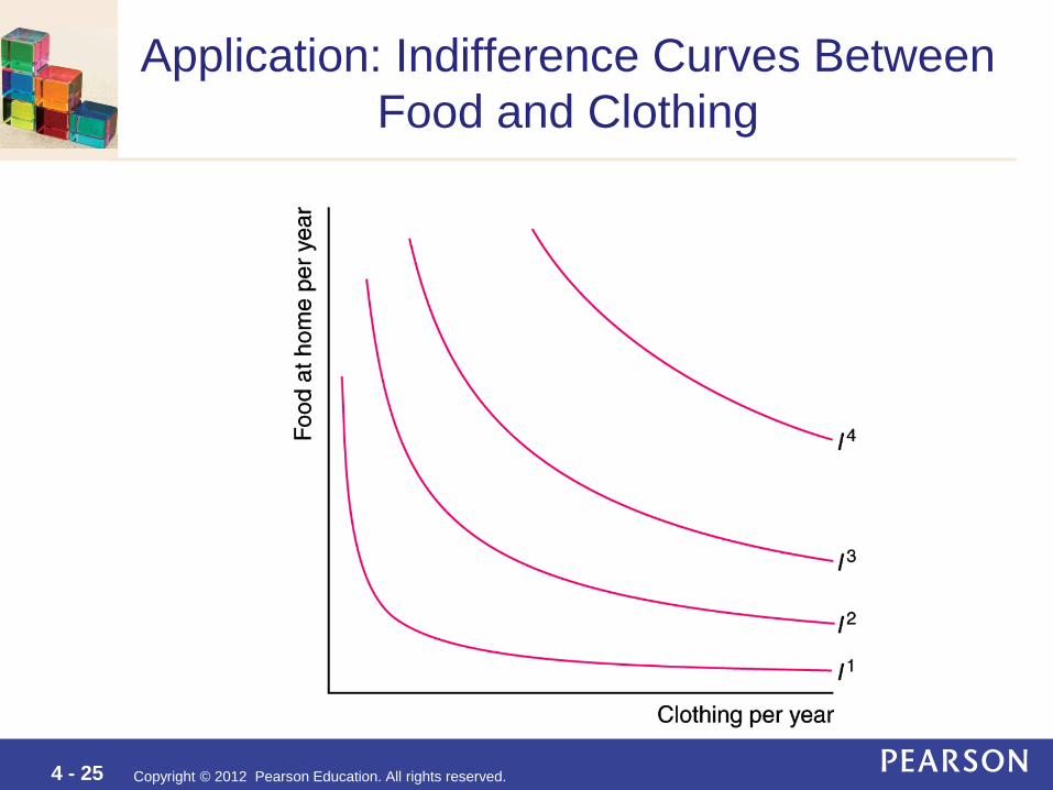
Application: Indifference Curves Between Food and Clothing
Copyright © 2012 Pearson Education. All rights reserved. 4 - 26
Problems: Constructing Indifference Curves
1. Don is altruistic. Show the possible shape of his indifference curves between charity and all other goods.
2. Miguel considers tickets to the Houston Grand Opera and to Houston Astros baseball games to be perfect substitutes. Show his preference map.
3. If Joe views two candy bars and one piece of cake as perfect substitutes, what is his marginal rate of substitution between candy bars and cake?
Copyright © 2012 Pearson Education. All rights reserved. 4 - 27
Utility
• Utility - a set of numerical values that reflect the relative rankings of various bundles of goods.
• Utility function - the relationship between utility values and every possible bundle of goods:
U(Z, B)
Copyright © 2012 Pearson Education. All rights reserved. 4 - 28 Copyright © 2012 Pearson Addison-Wesley. All rights reserved.
Utility Function: Example
BZBZU =),(
Copyright © 2012 Pearson Education. All rights reserved. 4 - 29
Ordinal Preferences
• If we only know a consumer’s relative ranking of bundles, the measure of pleasure is ordinal. Tells us the relative ranking of two things but
not how much more one rank is than another (letter grades).
• A cardinal measure is one by which absolute comparisons between ranks may be made (money).
Copyright © 2012 Pearson Education. All rights reserved. 4 - 30
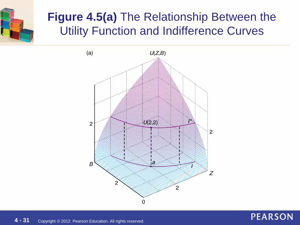
Utility and Indifference Curves
• An indifference curve consists of all those bundles that correspond to a particular level of utility.
• If Lisa’s utility function is U(Z, B), then an indifference curve is given by
Copyright © 2012 Pearson Education. All rights reserved. 4 - 31
Figure 4.5(a) The Relationship Between the Utility Function and Indifference Curves
Copyright © 2012 Pearson Education. All rights reserved. 4 - 32
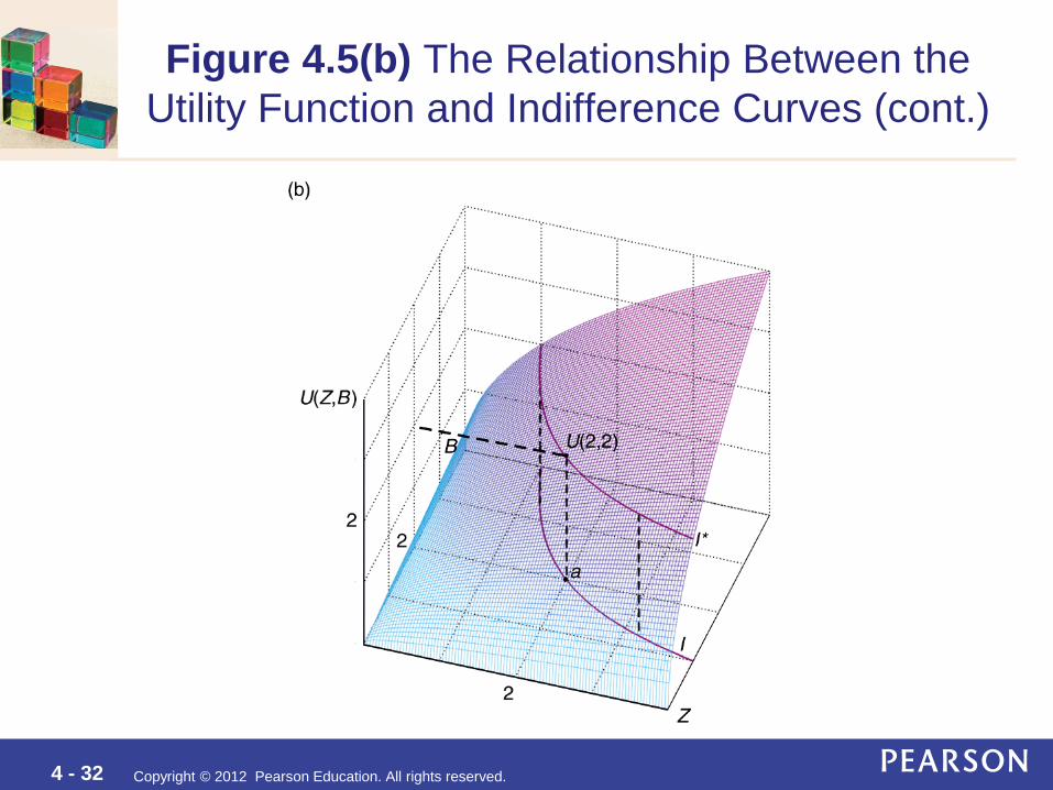
Figure 4.5(b) The Relationship Between the Utility Function and Indifference Curves (cont.)

Copyright © 2012 Pearson Education. All rights reserved. 4 - 33
Marginal Utility
• Marginal utility - the extra utility that a consumer gets from consuming the last unit of a good. the slope of the utility function as we hold the
quantity of the other good constant.
• Marginal utility of good Z is:
ZUMUZ ∆
∆=

Copyright © 2012 Pearson Education. All rights reserved. 4 - 34
Figure 4.6 Utility and Marginal
Utility • As Lisa consumes
more pizza, holding her consumption of burritos constant at 10, her total utility, U, increases… and her marginal
utility of pizza, MUZ, decreases (though it remains positive).
• Marginal utility is the
slope of the utility function as we hold the quantity of the other good constant.
MU
Z , M
argi
nal u
tility
of p
izza
MU Z
10 9 8 7 6 5 4 3 2 1 Z , Pizzas per semester
0
130
(b) Marginal Utility
20
U , U
tils
∆U = 20
Utility function, U (10, Z )
∆Z = 1
10 9 8 7 6 5 4 3 2 1 Z , Pizzas per semester
0
350
250
(a) Utility
230 ZUMUZ ∆
∆=
Copyright © 2012 Pearson Education. All rights reserved. 4 - 35
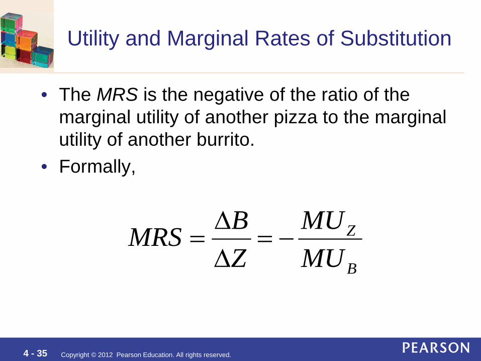
Utility and Marginal Rates of Substitution
• The MRS is the negative of the ratio of the marginal utility of another pizza to the marginal utility of another burrito.
• Formally,
B
Z
MUMU
ZBMRS −=
∆∆
=

Copyright © 2012 Pearson Education. All rights reserved. 4 - 36
Budget Constraint
• Budget line (or budget constraint) - the bundles of goods that can be bought if the entire budget is spent on those goods at given prices.
• Opportunity set - all the bundles a consumer can buy, including all the bundles inside the budget constraint and on the budget constraint.
Copyright © 2012 Pearson Education. All rights reserved. 4 - 37
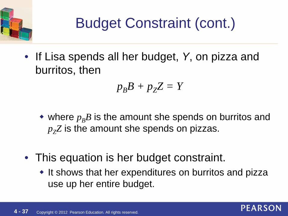
Budget Constraint (cont.)
• If Lisa spends all her budget, Y, on pizza and burritos, then
pBB + pZZ = Y
where pBB is the amount she spends on burritos and pZZ is the amount she spends on pizzas.
• This equation is her budget constraint. It shows that her expenditures on burritos and pizza
use up her entire budget.
Copyright © 2012 Pearson Education. All rights reserved. 4 - 38
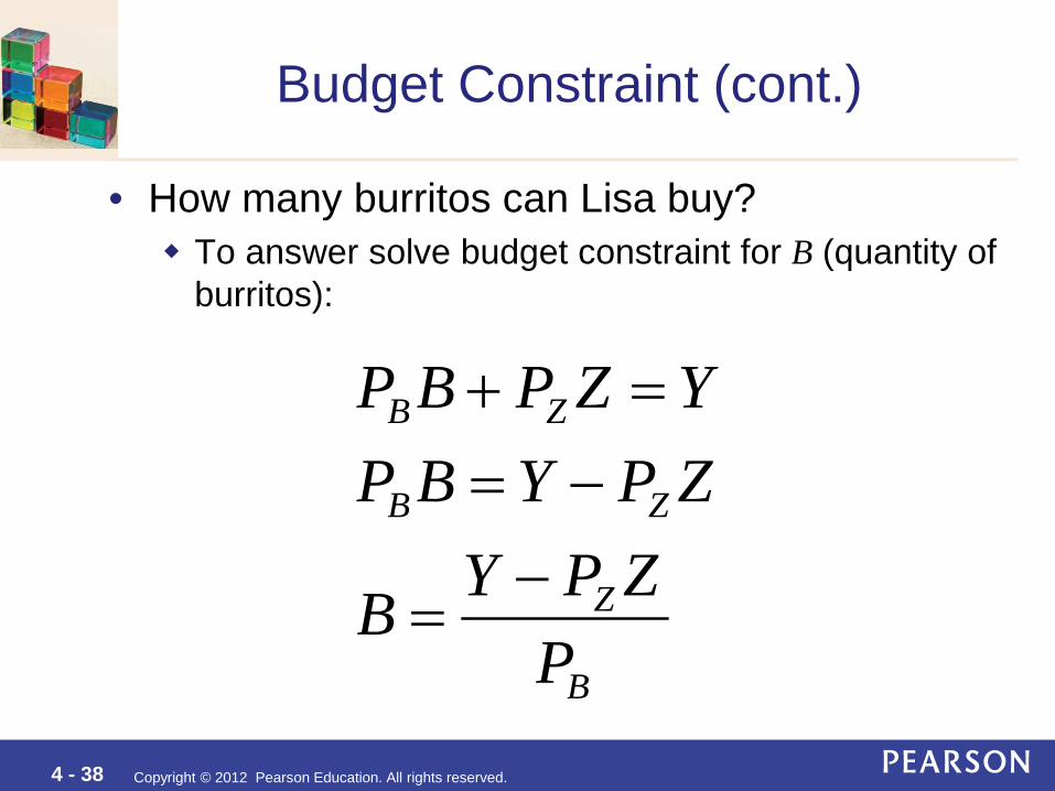
Budget Constraint (cont.)
• How many burritos can Lisa buy? To answer solve budget constraint for B (quantity of
burritos):
B
Z
ZB
ZB
PZPYB
ZPYBPYZPBP
−=
−==+
Copyright © 2012 Pearson Education. All rights reserved. 4 - 39
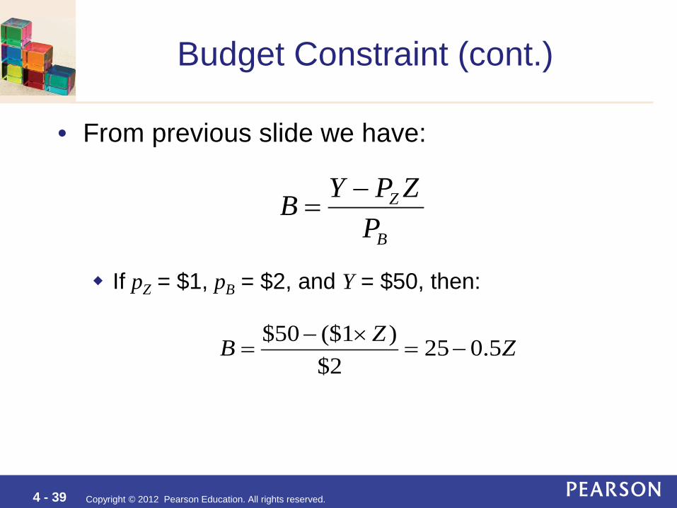
Budget Constraint (cont.)
• From previous slide we have: If pZ = $1, pB = $2, and Y = $50, then:
B
Z
PZPYB −
=
$50 ($1 ) 25 0.5$2
ZB Z− ×= = −

Copyright © 2012 Pearson Education. All rights reserved. 4 - 40
Table 4.1 Allocations of a $50 Budget Between Burritos and Pizza

Copyright © 2012 Pearson Education. All rights reserved. 4 - 41
Figure 4.7 Budget Constraint
From previous slide we have that if:
– pZ = $1, pB = $2, and Y = $50, then the budget constraint, L1, is:
$50 ($1 ) 25 0.5$2
ZB Z− ×= = −
B , B
ur r it
os p
er s
emes
ter
Opportunity set
50 = Y / p Z
L 1
25 = Y / p B
20
10
10 0 30 Z , Pizzas per semester
a
b
c
d
Amount of Burritos consumed if all income is allocated for Burritos.
Amount of Pizza consumed if all income is allocated for Pizza.

Copyright © 2012 Pearson Education. All rights reserved. 4 - 42
The Slope of the Budget Constraint
• We have seen that the budget constraint for Lisa is given by the following equation: The slope of the budget line is also called the marginal rate of
transformation (MRT) • rate at which Lisa can trade burritos for pizza in the marketplace
ZPP
PYB
B
Z
B
−=
Slope = ∆ B/∆ Z = MRT
Copyright © 2012 Pearson Education. All rights reserved. 4 - 43
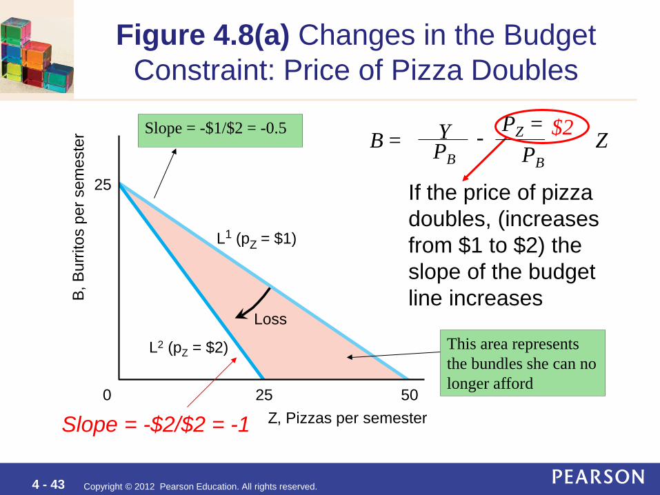
Figure 4.8(a) Changes in the Budget Constraint: Price of Pizza Doubles
B , B
ur r it
os p
er s
emes
ter
Loss
50
L 1 ( p Z = $1)
L2 (pZ = $2)
25
25 0 Z , Pizzas per semester
B = Y PB
- PZ = $1 PB
Z
If the price of pizza doubles, (increases from $1 to $2) the slope of the budget line increases
This area represents the bundles she can no longer afford
$2 Slope = -$1/$2 = -0.5
Slope = -$2/$2 = -1

Copyright © 2012 Pearson Education. All rights reserved. 4 - 44
Figure 4.8(b) Changes in the Budget Constraint: Income Doubles
Gain
L 3 ( Y = $100)
L 1 ( Y = $50)
0
B = $50 PB
- PZ PB
Z
If Lisa’s income increases by $50 the budget line shifts to the right (with the same slope!)
$100
This area represents the new consumption bundles she can now afford!!!
100 50 Z , Pizzas per semester
B, B
urrit
os p
er s
emes
ter
50
25
Copyright © 2012 Pearson Education. All rights reserved. 4 - 45
Solved Problem 4.3
• A government rations water, setting a quota on how much a consumer can purchase. If a consumer can afford to buy 12 thousand gallons a month but the government restricts purchases to no more than 10 thousand gallons a month, how does the consumer’s opportunity set change?

Copyright © 2012 Pearson Education. All rights reserved. 4 - 46
Solved Problem 4.3

Copyright © 2012 Pearson Education. All rights reserved. 4 - 47
Constrained Consumer Choice
• Given information on Lisa’s preferences and her budget, we can determine her optimal bundle.
• Her optimal bundle is the bundle out of all the bundles that she can afford that gives her the most pleasure.
Copyright © 2012 Pearson Education. All rights reserved. 4 - 48
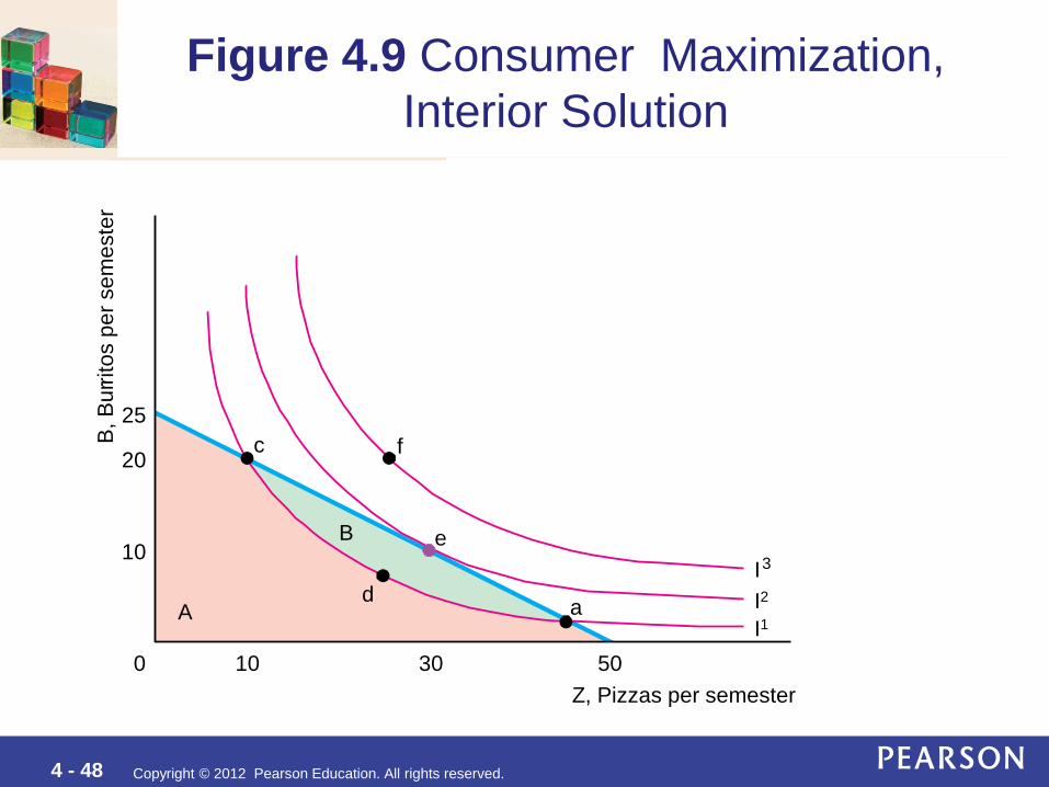
Figure 4.9 Consumer Maximization, Interior Solution
• Would Lisa be able to consume any bundle along I3 (i.e. bundle f)? No! Lisa does not have
enough income to afford any bundle along I3
B , B
ur r it
os p
er s
emes
ter
10
20
25
50 30 10 0 Z , Pizzas per semester
I1 I2
I 3
d
f c
e
a A
B
Would Lisa be able to consume any bundle along I1? Yes; she could afford bundles
d, c, and a. Nevertheless, there are other
affordable bundles that should be preferred and affordable. For instance bundle e
Bundle e is called a consumer’s optimum. If Lisa is consuming this
bundle, she has no incentive to change her behavior by substituting one good for another.
Copyright © 2012 Pearson Education. All rights reserved. 4 - 49
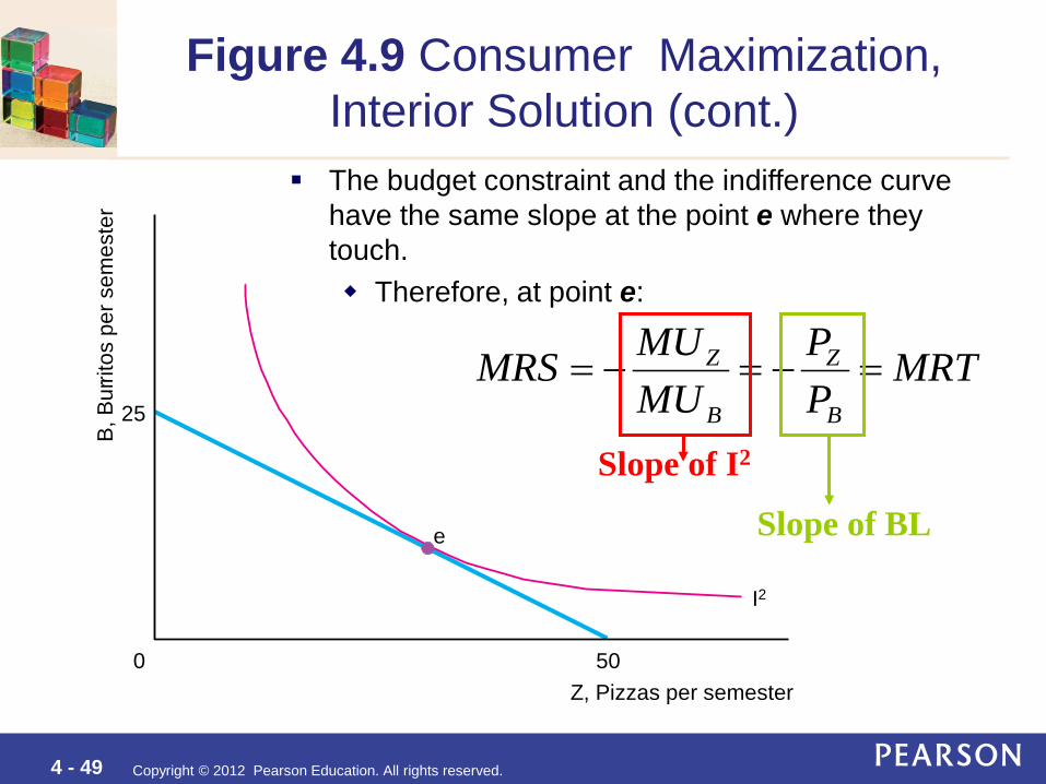
The budget constraint and the indifference curve have the same slope at the point e where they touch. Therefore, at point e:
Slope of I2
Figure 4.9 Consumer Maximization, Interior Solution (cont.)
B , B
ur r it
os p
er s
emes
ter
25
50 0 Z , Pizzas per semester
I2
e
MRTPP
MUMUMRS
B
Z
B
Z =−=−=
Slope of BL

Copyright © 2012 Pearson Education. All rights reserved. 4 - 50
Figure 4.10 Consumer Maximization, Corner Solution
B , B
ur r it
os p
er s
emes
ter
Budget line
25
50 Z , Pizzas per semester
I 1
I 2
I 3
e

Copyright © 2012 Pearson Education. All rights reserved. 4 - 51
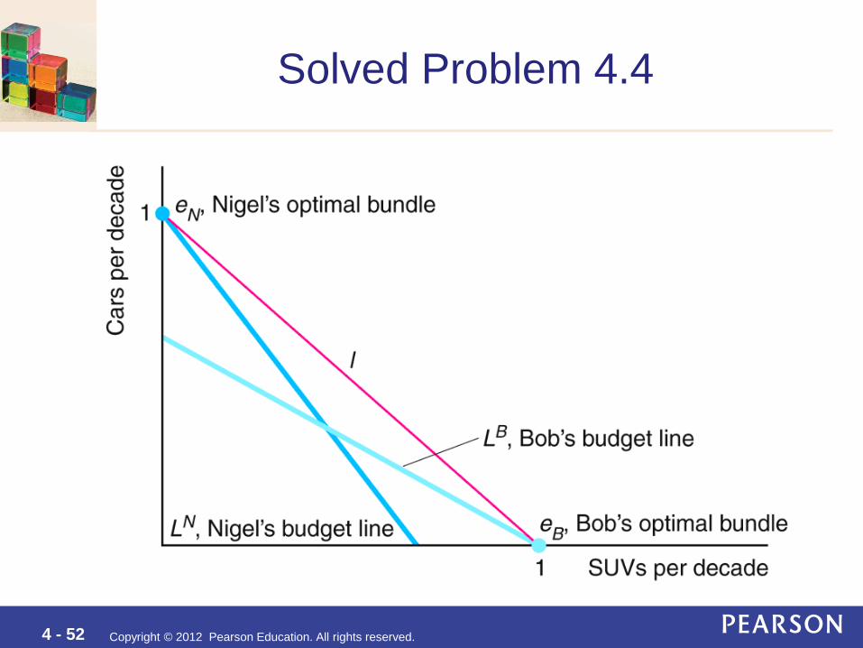
Solved Problem 4.4
• Nigel, a Brit, and Bob, a Yank, have the same tastes, and both are indifferent between a sports utility vehicle (SUV) and a luxury sedan. Each has a budget that will allow him to buy and operate one vehicle for a decade. For Nigel, the price of owning and operating an SUV is greater than that for the car. For Bob, an SUV is a relative bargain because he benefits from lower gas prices and can qualify for an SUV tax break. Use an indifference curve–budget line analysis to explain why Nigel buys and operates a car while Bob chooses an SUV.
Copyright © 2012 Pearson Education. All rights reserved. 4 - 52
Solved Problem 4.4

Copyright © 2012 Pearson Education. All rights reserved. 4 - 53
Figure 4.11 Optimal Bundles on Convex Sections of Indifference Curves
Copyright © 2012 Pearson Education. All rights reserved. 4 - 54
Food Stamps
• Renamed to Supplemental Nutrition Assistance Program (SNAP) in 2008.
• Nearly 11% of U.S. households worry about having enough money to buy food and 4.1% report that they suffer from inadequate food (U.S. Department of Agriculture, 2008).
• Households that meet income, asset, and employment eligibility requirements receive coupons that can be used to purchase food from retail stores.
Copyright © 2012 Pearson Education. All rights reserved. 4 - 55
Food Stamps (cont.)
• SNAP is one of the nation’s largest social welfare programs with expenditures of $73 billion for nearly 40 million people in 2010.
• Would a switch to a comparable cash subsidy increase the well-being of food stamp recipients? Would the recipients spend less on food and
more on other goods?

Copyright © 2012 Pearson Education. All rights reserved. 4 - 56
Figure 4.12 Food Stamps Versus Cash
All o
ther
goo
ds p
er m
onth
Y Y + 100
Y + 100
0 100 F ood per month
Budget line with f ood stamps
Budget line with cash
O r iginal b udget line
A
B
f
d e Y
C
I 1
I 2 I 3
Copyright © 2012 Pearson Education. All rights reserved. 4 - 57
Behavioral Economics
• By adding insights from psychology and empirical research on human cognition and emotional biases to the rational economic model, economists try to better predict economic decision making.
Copyright © 2012 Pearson Education. All rights reserved. 4 - 58
Test of Transitivity
• Adults tend to make transitive choices. • Children are less likely to make transitive
choices.

Copyright © 2012 Pearson Education. All rights reserved. 4 - 59
Endowment Effect
• People place a higher value on a good if they own it than they do if they are considering buying it.
• Consumer choice theory assumes a consumer’s endowment does not affect the indifference curve map.
• Research has shown that experience significantly reduces the endowment effect.
Copyright © 2012 Pearson Education. All rights reserved. 4 - 60
Salience
• People are more likely to consider information if it is presented in a way that grabs their attention or if it takes relatively little thought or calculation to understand.

Copyright © 2012 Pearson Education. All rights reserved. 4 - 61
Salience (cont.)
• When a stores posted prices exclude the sales tax, consumer are much less likely to react to a change in the price.
• Tax is not salient and some consumers ignore taxes.
• Bounded rationality - people have a limited capacity to anticipate, solve complex problems, or enumerate all options.