chapter 4. statics of plate o classical linear theory of
TRANSCRIPT

Chapter 4. Statics of Plate
o Classical Linear Theory of Plate
o Plane stress and Plane strain
o Equations of Equilibrium and Boundary Conditions
- Equilibrium Approach
- Minimum Potential Energy Approach-Thin plate
o Solution methods
etc
Basic Assumptions
~In the initial state, the surfaces of a flat plate are parallel planes,
called the faces of the plate
~The distance between the faces is called the thickness of the plate.
~A plate is distinguished from a block by the fact that the thickness is small
compared to the dimensions paralled to the faces.
~The plane midway between the faces is called the middle plane of the plates
~The bending properties of plate depend greatly on its thickness as compared
with its other dimensions.
:We will discuss the linear static theory of thin elastic plate in this chapter.
~ shell ? membrane ? plate ?

4.1 Classical linear theory of plate
Definition of small deformation : :1w
h
Decoupled set of Bending and stretching ~ Isotropic material
~ Homogeneous materials
~ Isotropic or Anisotropic(Composite)
~ Thick plate : 1 1/ ~
20 10h l Thin plate 1
/20
h l
~ Loading :
o Bending action ~ deflection
o Membrane action~stretching
Configuration of curved surface ~

Displacements :
~ ( 1 , 2 ) ,( , ) , ( , ) , ( , )u wu x y v x y w x y
: In-plane displacements ,u v ~ deflection w
3-Dimensional linear elasticity
,i j j jq
For plate bending problem, let
0( 1,2)q

~
, 3,3
3 , 33,3 3
: 0
:
u
w F
with boundary conditions !
4-1-1 Kinematics of Deformation
The fundamental assumptions of the small deflection theory of bending or so
called classical theory of isotropic homogeneous elastic thin plate
; Kirchhoff – Love hypothesis material property change
Kinematic Assumptions

1. Deflection of mid-surface is small compared with the thickness of the plate.
: Slope of the deflected surface is very small and the square of the slope is a
negligible quantity in comparison with unity
2.The mid-plane remains unstrained subsequent to bending
# Large deflection case ?
3. Plane sections initially normal to surface remains plane and normal to that
surface after the bending : 0( 1,2)~ ~z
G
Before bending ~> After bending ?
? Higher-order theory
? Thick plate theory ~ Mindlin plate theory

4. No stretching or contraction of normal : 0zz
5.The stress normal to the mid-plane, :zz
small compared with the other stress
components and may be neglected
: This assumption becomes unreliable in the vicinity of highly concentracted
transverse loads.
0 1 2 2
0 1 2 2
3 3 3 3
( , ) ( , ) ( , ) ( , ) . . .
0
( , ) ( , ) ( , ) ( , ) . . .30
( , , ) ( , )
( , , ) ( , )
m m
m m
m mu x y z u x y u x y z u x y z
m
m mu x y z u x y u x y z u x y z
m
u x y z u x y z
w x y z u x y z
~ order of thickness effects !
3
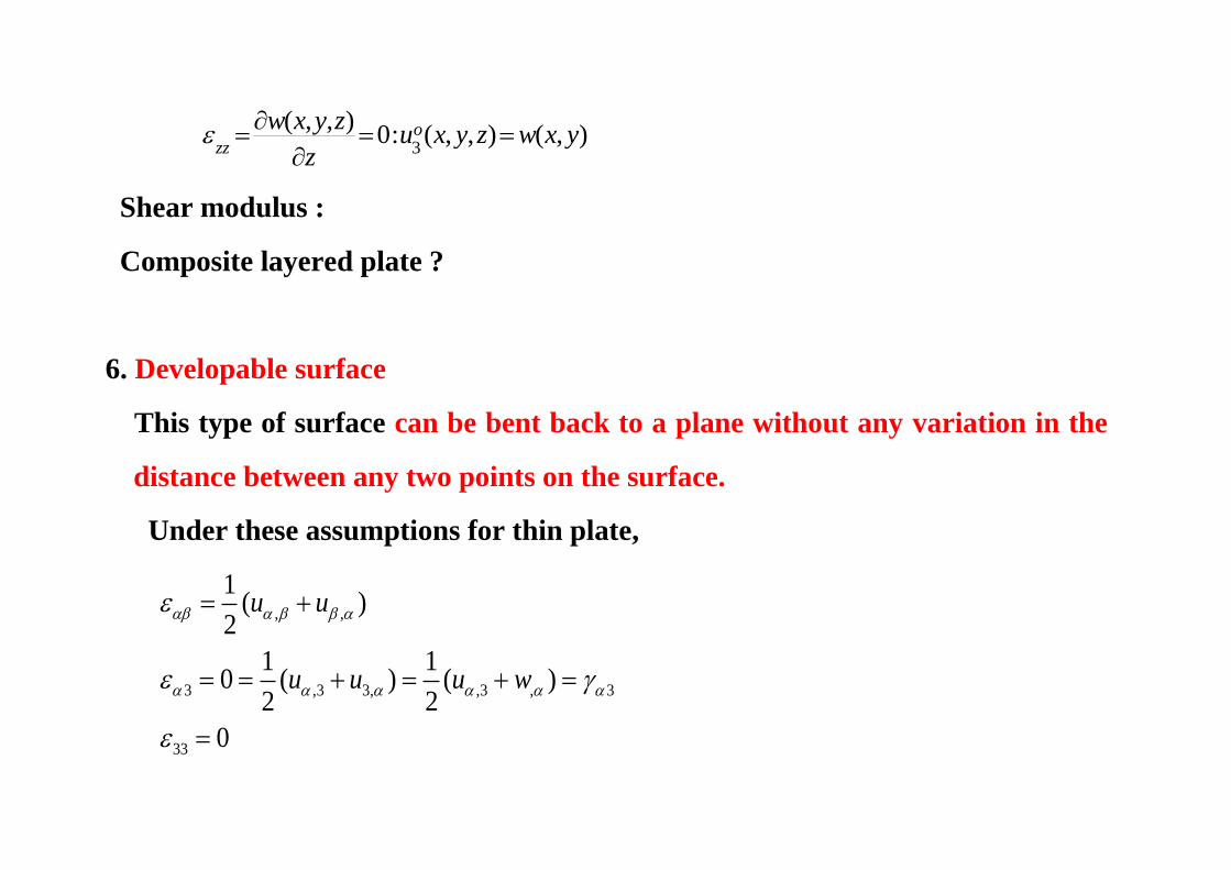
( , , )0: ( , , ) ( , )o
zz
w x y zu x y z w x y
z
Shear modulus :
Composite layered plate ?
6. Developable surface
This type of surface can be bent back to a plane without any variation in the
distance between any two points on the surface.
Under these assumptions for thin plate,
, ,
3 ,3 3, ,3 , 3
33
1( )
2
1 10 ( ) ( )
2 2
0
u u
u u u w

3 ,3 ,
,3 ,
,
1( ) 0,
2
:
~
( , , ) ( , )
:
?
u w
u w
u x y z u x y zw
4-1.2. Plane stress and Plane strain
For 3 D elasticity theory:
2
: ,2(1 ) (1 )(1 2 )
ij ll ijG
E Ewith G

Plane stress field for kinematic assumptions of 3 33
0
( )1 1
E
~ ( , ) 0Load Geometry
z
(i) Thin flat plate
(ii) Applied load are acting on the xy surfaces and do not vary
across the thickness.
(iii) Upper and lower surface are stress free 0zz z
~ iz
through thickness.
(iv) do not vary across the thickness

Plane strain
Dimension of z >> dimension of x,y
iz
0
4-1.3. Equation of Equilibrium & Boundary Conditions
3D ~> plate theory ?
3 :x Elimination of explicit dependency !

Stress, Moment resultants
1
23
2
, ) (1, )( h z dxN M
, : ?
: ?
xx yy
xy
M M
M
Shear force intensity
2
3 3
2
h
h dxQ
According to basic assumptions and plane stress assumption,
3 0i

0,
3
( , , ) ( , ) ( , )
( , , ) ( , )
u x y z u x y z w x y
u x y z w x y
Total number of independent displacement components ?
0 0, , , ,
1( ) ( )
2 2
zu u w w
~ (1, )~ :(1, )z z
A . Equilibrium Approach
3-D elasticity (without body force)
, 3 , 3
3 , 3 3 , 3
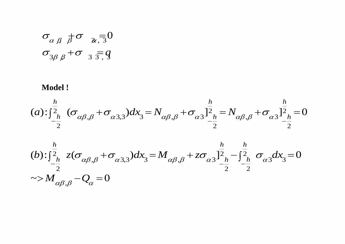
0
q
Model !
2 22, 3,3 3 , 3 , 3
2 2 2
22 2, 3,3 3 , 3 3 3
2 22
,
( ): ( ) ] ] 0
( ): ( ) ] 0
~ 0
h hh
h h h
hh h
h hh
a dx N N
b z dx M z dx
M Q

(c)
223 , 33,3 3 , 33
2 2
, 33 332 2
,
( ) ] 0
~ ( ) ( ) 0
: 0
hh
h h
h h
dx Q
Q
Q q
Substitute Eq.(b) into Eq.(c)

,0M q
Finally,
, , ,
, ,
, ,
2
0
0
xx xx xy xy yy yy
xx x xy y
yx x yy y
M M M q
N N
N N
Equations may be coupled set.
For isotropic plate,

Membrane stretching effect and Bending effect: Decoupled
Mid-plane ?
For rectangular plate:
Obtain stress field in terms of strain components
Obtain N,M in terms of u,v,w
…
then, ;
Bending problem; 4th
order eqn.( Hermite approximation:C1 continuity)
4,
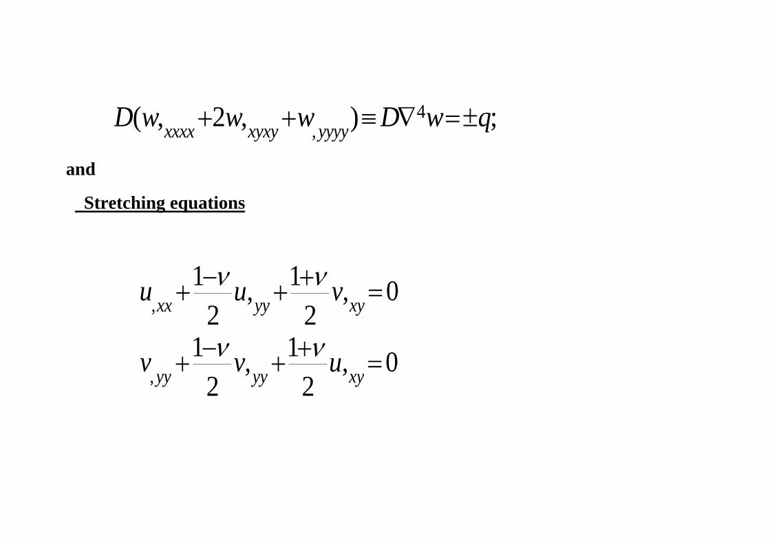
( , 2 , ) ;xxxx xyxy yyyy
D w w w D w q
and
Stretching equations
,
,
1 1, , 0
2 21 1
, , 02 2
xx yy xy
yy yy xy
u u v
v v u

% ,0M Q
, ,
2, ,
~
2 ,
( , , (1 ) , )
( , , ) ( , , ) ( )
( )
xyyx xx x xy y xxx yyx
xxx xyy xx yy x x
yy
Q M M D w w w
D w w D w w D w
Q D w
B. Minimum Potential Energy Approach
~ Strain energy of entire plate with linear elastic behavior

2
( )
2
1
2
h
ij ijihA
U dzdA
Replacing ij in terms of ij in conjunction with plane stress state
2
( ) 2
2
2 2 2 2
2
2
1
2(1 )
12 2(1 )
2(1 )
h
ihA
h
xx xx yy yy xyhA
U dzdA
dzdA

Potential energy for the external load
( )( , ) ( , )
e AU q x y w x y dA
Remembering, 0 ,u u zw
and , ,
1( )
2u u
2 0 2 2 2
, ,( ) 2
2
1( ) 2 2(1 )
2(1 )
h
x xx xx yy yy xyihA
U u zw dzdA
Total potential energy
( ) ( ) ( )( , ) ( , )
i e i AU U U U q x y w x y dA

Integrating by part with respect to z:
(~ Extensional energy + Bending Energy ! )
( ) ( ) ( )m B
i i iU U U
where,
0 0( ) ( )
( , ), ( )m Bi i
U u v U w
: Decoupling ! ?
Obtain the expression & govering eqn for (Report !)

We shall be concerned with the stresses and moments in plates as a result of
transverse loadings of bending part
( ) ( )
2 2 2 2,( )
2
~ ( ) 2(1 )[ , , ]2
m Bi i
h
Bxy xx yyi
hA A
U U U
DU w w w w dA qwdA
To extremize this functional, we get
0U

2 2 2 2
,
2
[ ( ) 2(1 )[ , , ] ]2
h
xy xx yyhA A
Dw w w w dA qwdA
2 2
,
2 2
, ,
2 2
, ,
,
2( ) 2(1 )[2 , , , , , ]2
2( ) (1 )[2( , , )2
2 , , 2 , , ]
( ) (1 )[2( , , )
2 , , 2 , , ]
( ,
xy xy xx yy xx yy
xy xy yx yx
xx yy xx yy
xy xy yx yx
xx yy xx yy
xx x
Dw w w w w w w w dA
Dw w w w w w
w w w w dA
D w w w w w w
w w w w dA
D w w
,
, ,
, ) ( , , , ,
(1 )( , , )]
x yy yy yy xx xx yy
xy xy yx yx
w w w w w w
w w w w dA

Using Green’s formula(Report!)
4( ) ..... 0D w q w dA D
Introducing the moment intensity, then the above equation becomes(Report)
4
, ,( ) , ......... ( ) 0xx x xx x xy yD w q w dA M w dy M M wdy
We may rewrite the last two integrals in terms of shear force intensities.
We then have ( Report )

4( ) , ......... 0xx x xD w q w dA M w dy Q wdy
To simplify this functional further, let introduce the coordinate n, s which are
the normal and tangential directions to contour, respectively.
Then ( Report )…
4( ) . 0nn ns n
w wD w q w dxdy M ds M ds Q wds
n s
The 3rd
integral becomes, by integration by parts

...(?)nsns
MwM ds wds
s s
We then get for the variation of the total potential
4( ) ( ) 0nsnn n
MwD w q w dA M ds Q wds
n s
Euler-Lagrange equation for this problem is
4D w q
Report :Derive the governing equation with with variable bending rigidity

which have been derived in previous section. Now we get as a result of the
variational process two sets of boudary conditions, namely, the natural and the
kinematic bound conditions.
Then on the boundary we require that
(a)
0.. .. .. ..nn
wM or is prescribed
n
(b)
0.. .. .. ..nsn
MQ or w is prescribed
s
There are only 2 conditions, in spite of the fact the there 3 variables

, ,nn n nsM Q M
The 1st condition is acceptable by physical consideration and needs no
further comment.
We shall now examine the 2nd
condition with the view reaching some
physical explanation. :
We have shown part of the edge of the plate when two panels of length S
have been identified.
_ Figure_
The twisting moments have been expressed in the first and second panel. A
third panel of length S may be imagined the center of two panels, which is
shown in Fig AB. The shear force for thin panel is shown as nQ S .

Now we make use of the Saint-Venant principle by replacing the twisting
moment distribution of the original two panels by two couples having forces
value nsM and ns
ns
MM
s
respectively with a distance of S between the
forces as shown in the figure.
Clearly, any conclusion arising from the new arrangement valid away from
the edege. Now we focus on attention on the central panel AB. The effective
shear force intensity, effQ for this panel is then seen to be
1[ ( ) ]ns ns
eff n ns ns n
M MQ Q S M S M Q
S s s

We may now say that the 2nd
of our natural boundary conditions renders the
effective shear force intensity equation to zero. From the above equations we
can see that the difference nsM
s
does work in the same manner as nQ and
these two effect cannot distinguished.
The force per unit length, nsM
s
is called Kirchhoff supplementary force.
This explanation is by Thomson and Tait.
Because we employed a constitutive equation, Hook law, in the formulation it
might seem that the natural boundary conditions are restricted to Hookean
material.
In the next section, no constitutive law is used and we will derive the general
moment intensity and shear force intensity equations present in Sec.3.1.3.a

4.1.3.c.(Thin Plate) Virtual work Approach (Rectangular plate)
In using the principle of virtual work, we shall consider a rectangular plate.
In particular we shall examine closely the corner condition for such a problem.
We now apply the principle of virtual work, under the assumption of plane
stress, to a rectangular plane having dimensions a b h and loaded normal to
the middle-plane of the plate by a loading intensity ( , )q x y .
If body forces are absent,
2
0 0 0 0
2
h
a b a b
h
q wdxdy dxdy

Considering only bending contribution, then by , ,
ou zw ( thin plate
assumption)
we got
2
0 0
2
,
h
a b
h
z w dxdy
0 0
0
a b
q wdxdy
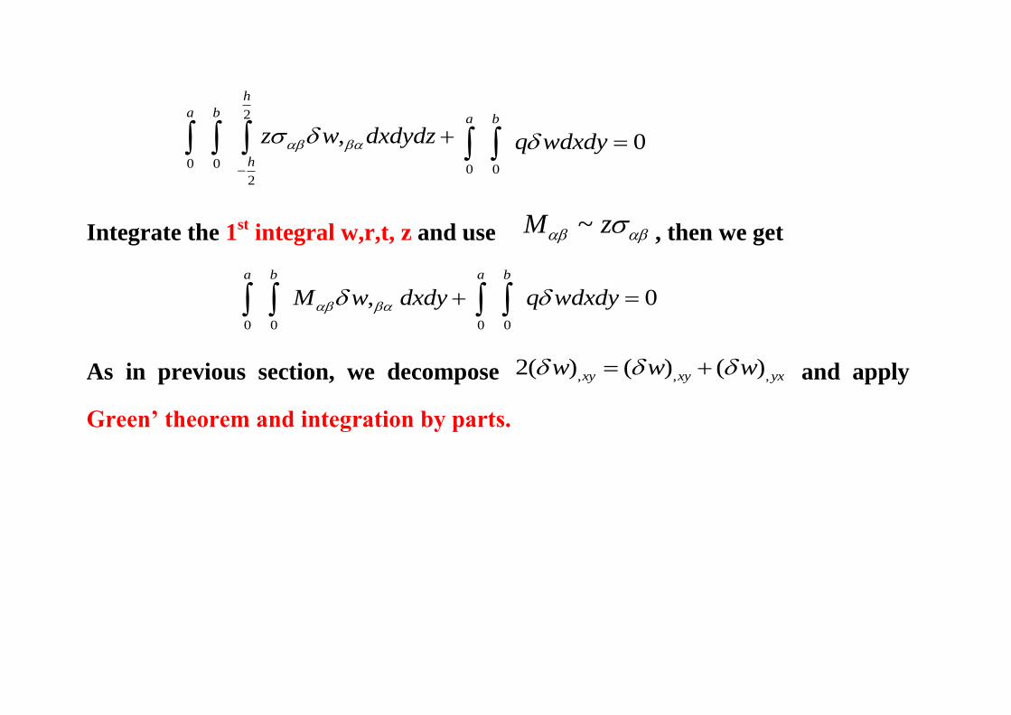
Integrate the 1st integral w,r,t, z and use ~M z , then we get
2
0 0
2
,
h
a b
h
M w dxdy
0 0
0
a b
q wdxdy
As in previous section, we decompose , , ,2( ) ( ) ( )xy xy yxw w w and apply
Green’ theorem and integration by parts.

2
, , 0 , 0
0 0 0 0
2
, , 0 , , 0
0 0
, 0 , 0
0 0
( ) ( ) ] ( ) ]
( ) ] ( ) ]
( ( ) ] ( ( ) ] 0
h
a b b a
a b
xx x yy y
h
b a
a b
xx x xy y yy y xy x
a b
b a
xy x xy y
M q wdxdy M w dy M w dx
M M w dy M M w dx
M w dx M w dy
Now, integrate the last two integrate by part, then we obtain
, 0 0 0 , 0
0 0
, 0
0
( ( ) ] [( ] ] ]
( ( ) ] ?
a a
b y b x a b
xy x xy y x xy x
b
a
xy y
M w dx M w M w dx
M w dy

Inserting these results and noting ~ .. ..Q derivative of M , we get
2
, , 0 , 0
0 0 0 0
2
, 0 , 0
0 0
, 0, ,0 0,0
( ) ( ) ] ( ) ]
( ) ] ( ) ]
2( ) 2( ) 2( ) 2( )
0
h
a b b a
a b
xx x yy y
h
b a
a b
x xy y y xy x
xy a b xy b xy a xy
M q wdxdy M w dy M w dx
Q M w dy Q M w dx
M w M w M w M w
...(?)nsns
MwM ds wds
s s

We then get for the variation of the total potential
4( ) ( ) 0nsnn n
MwD w q w dA M ds Q wds
n s
Euler-Lagrange equation for this problem is
4D w q
Report :Derive the governing equation with variable bending rigidity
which have been derived in previous section. Now we get as a result of the
variational process two sets of boudary conditions, namely, the natural and the
kinematic bound conditions.

Then on the boundary we require that
(a)
0.. .. .. ..nn
wM or is prescribed
n
(b)
0.. .. .. ..nsn
MQ or w is prescribed
s
There are only 2 conditions, in spite of the fact the there 3 variables
, ,nn n nsM Q M
The 1st condition is acceptable by physical consideration and needs no
further comment.
We shall now examine the 2nd
condition with the view reaching some

physical explanation. :
We have shown part of the edge of the plate when two panels of length S
have been identified.
_ Figure_
The twisting moments have been expressed in the first and second panel. A
third panel of length S may be imagined the center of two panels, which is
shown in Fig AB. The shear force for thin panel is shown as nQ S .
Use of the Saint-Venant principle : by replacing the twisting moment
distribution of the original two panels by two couples having forces value nsM
and ns
ns
MM s
s
respectively with a distance of S between the forces as

shown in the figure.
Clearly, any conclusion arising from the new arrangement valid away from
the edege. Now we focus on attention on the central panel AB. The effective
shear force intensity, effQ for this panel is then seen to be
1[ ( ) ]ns ns
eff n ns ns n
M MQ Q S M S M Q
S s s
We may now say that the 2nd
of our natural boundary conditions renders the
effective shear force intensity equation to zero. From the above equations we
can see that the difference nsM
s
does work in the same manner as nQ and

these two effect cannot distinguished.
The force per unit length, nsM
s
is called Kirchhoff supplementary force.
This explanation is by Thomson and Tait.
Because we employed a constitutive equation, Hook law, in the formulation it
might seem that the natural boundary conditions are restricted to Hookean
material.
In the next section, no constitutive law is used and we will derive the general
moment intensity and shear force intensity equations present in Sec.3.1.3.a
4.1.3.c.(Thin Plate) Virtual work Approach (Rectangular plate)
In using the principle of virtual work, we shall consider a rectangular plate.

In particular we shall examine closely the corner condition for such a problem.
We now apply the principle of virtual work, under the assumption of plane
stress, to a rectangular plane having dimensions a b h and loaded normal to
the middle-plane of the plate by a loading intensity ( , )q x y .
If body forces are absent,
2
0 0 0 0
2
h
a b a b
h
q wdxdy dxdy
Considering only bending contribution, then by , ,
ou zw ( thin plate
assumption)
we got
2
0 0
2
,
h
a b
h
z w dxdydz
0 0
0
a b
q wdxdy
Integrate the 1st integral w,r,t, z and use ~M z , then we get
0 0
,
a b
M w dxdy 0 0
0
a b
q wdxdy
As in previous section, we decompose , , ,2( ) ( ) ( )xy xy yxw w w and apply
Green’ theorem and integration by parts.

, , 0 , 0
0 0 0 0
, , 0 , , 0
0 0
, 0 , 0
0 0
( ) ( ) ] ( ) ]
( ) ] ( ) ]
( ( ) ] ( ( ) ] 0
a b b a
a b
xx x yy y
b a
a b
xx x xy y yy y xy x
a b
b a
xy x xy y
M q wdxdy M w dy M w dx
M M w dy M M w dx
M w dx M w dy
Now, integrate the last two integrate by part, then we obtain
, 0 0 0 , 0
0 0
, 0
0
( ( ) ] [( ] ] ]
( ( ) ] ?
a a
b y b x a b
xy x xy y x xy x
b
a
xy y
M w dx M w M w dx
M w dy
Inserting these results and noting ~ .. ..Q derivative of M , we get

, , 0 , 0
0 0 0 0
, 0 , 0
0 0
, 0, ,0 0,0
( ) ( ) ] ( ) ]
( ) ] ( ) ]
2( ) 2( ) 2( ) 2( )
0
a b b a
a b
xx x yy y
b a
a b
x xy y y xy x
xy a b xy b xy a xy
M q wdxdy M w dy M w dx
Q M w dy Q M w dx
M w M w M w M w
Now we get from the above eqn,
, 0M q
~ Identical to the eqn by equilibrium approach ! valid for all mterials
On the boundary,

1) 0 x a
0 . . . . , rx x xM o r w p e s c r i b e d
, 0 . . . . rx x y yQ M o r w p e s c r i b e d
2) 0 y b
~~~~
Results: Same boundary conditions are appears as in Minimum total
potential energy.
Corner conditions ?

A Note on the Validity of the Classical Plate Theory
Now we have discussed fully for the classical theory of plate.
It seems to be the time to note the validity of the theory which we
have used the assumption of plane stress in the plate. By establishing
the order of magnitude of the stresses we can make comparisons as
follows. The transverse shears z are smaller by an order of h/L
( L: characteristic length of the middle plane) than the middle plane
shear ( ) . Also the transverse normal stress zz is smaller by
an order (h/L)2 than the middle plane normal stresses ( )( ) Thus

for a very thin plate h/L<<1/10, we have inner consistency and the
classical plate theory may be expected to give good results.
For a moderately thin plate, especially in the vicinity of concentrated
loads it might be well to account for the effects of transverse shear
deformation.
It is obvious from the equilibrium considerations that such stresses
will seldom be zero. Accordingly, we used assurance that the classical
plate theory, under proper conditions, yield meaningful results.

There are two approaches:
1. Compare with the results from a more exact theory
~ Theory of elasticity
2. Determine the bounds on the magnitude of stresses 3i that have
been deleted from the theory to show that these stresses, although
not zero, are nevertheless small compared to the stressesw.
In view of the scarcity of the exact solutions for plate bending
problem from 3-dimensional theory of elasticity, we shall follow the
latter procedure.
For this purpose,

, ,2
,
( ),1
?
1
xx xx yy
yy
xy xy
Ezw w
Ezw
Remember : , , ,
1 1~ ~ ( , ) ~ ( , )
2 2
o ou u u u zw
..xx xxM zdz etc

~ 3
,.. ?,.. ?
12
xxxx yy xy
M z
h
Now we use the stresses in the 3-D equilibrium equations
, 3ij j q
, , ,0 ~ 0xyxx xz
xx x xy y xz zx y z

, , ,3 3
( )
12 12
xz z xx x xy y x
z zM M Q
h h
Integrating w.r.t z
2
3
2( , ) ~ : : 0
2
12
3~ ( , ) /
2
~ ... ~ ...
xz x xz
x
xz yz
z
hQ f x y for z
h
f x y Q h
Similarly

Inserting ,xz yz into the third equation
, , ,
2 2
, ,2 2
~
3 4 3 4(1 )( ) (1 )
2 2
yzxzzzzz z xz x yz y
x x y y
z x y
z q zQ Q
h h h h
~>
3
2
3 4( ) ( , )
2 3
;2
: 02
zz
q zz g x y
h h
considering
hz q
hz

3
2
43 2
(~ ) ( ) ( , ) : ( , )2 2 3 2
zz
h
q h qq g x y g x y
h h
Finally,
2
2
3
2
3 4(1 )
2
?
3 4( )
2 3 2
xxz
yz
zz
Q z
h h
q z qz
h h
We have iz which are computed from equilibrium consideration

using results from a theory that neglected these very stresses.
If it turns out that the above computed stresses are small, we have inner
consistency in the theory.
To do so, we shall next make an order of magnitude study
Consider a portion of plate !
Figure ~

2( ) ( ) ( ) ( ) ( )O F O q O L O Q O L
Definition of shear force intensity ?
( ) ( ) ( ) ( )O Q O q O L O qL
Equate moments about an axis C-C’ going through the line of the
action of the resultant of the force distribution:
( ) ( ) ( ) ( ) ( ) ( ) ( ) 0sO Q O L O L O M O L O M O L

Replacing ( )O Q by using ( ) ( )O Q O qL
.
Assuming next that shear effects are as significant as either the
bending or the twisting effects.
If the resulting shear stresses turn out still to be small in our order
of magnitude studies.
We then equate the order of magnitude of bending and twisting with
That of the shear effect:
2 2( ) ( ), ( ) ( )sO M O qL O M O qL
We thus have order of magnitude formulations for the stress
resultant intensity functions, , sQ M M which may now be used in

conjunction with stresses for comparison purposes.
( ) ( )O z O h
2 2( ) ( / ), ( ) ..., ( ) ...xx xy yyO O qL h O O
2
2
3 1( ) ( (1 4 )) ( ) ( ) ( )
2
( ) ...
( ) ( )
xz x
yz
zz
z LO O Q O O qL O q
h h h h
O
O O q
We can now make comparisons :
Methods of Solution

Governing equations(A) ? + Boundary conditions(B) ?
Exact solution = A + B : Very special sets of Problems
Approximate solutions based on : Shape function:
~ Complete sets
Full domain :
Ritz method : Minimization of Potential Energy
Levy method
Galerkin’s method : Governing equations

Kantorovich method
Sub-domain~
FEM ? BEM ,XFEM …
4.2 Shear deformable plate theory
So far, theory of thin plate have been established based on Kirchhoff-Love
assumptions
In this section we shall consider the small deflection theory of thick plates

including the effect of transverse shear deformation which was neglected
despite of the fact that we know from equilibrium considerations that it was
not zero. This addition in our treatment of plates is analogous to the
Timoshenko beam theory.
In accordance with Reissner‟ theory we assume a linear law for distribution
of stresses σ𝑥𝑥 , σ𝑦𝑦 and σ𝑥𝑦 through the thickness of the plate. It may be
seen by replacing the bracked expression of the bending part in
, , , ,2 2( ) [ ( )]
1 1xx xx yy x y xx yy
E Eu v z
, , , ,2 2( ) [ ( )]
1 1yy yy xx y x yy xx
E Ev u z
, , ,
12 2 [ ( ) ]
2xy xy y x xyG G u v z
by bending moment and twisting moment intensities with the aid of
, ,( )x xx yyM D w w

, ,( )y yy xxM D w w
,(1 )xy yx xyM M Dw
Where 3
212(1 )
EhD
v
: bending rigidity of plates.
Derive 3
12 xxx
Mz
h ,
3
12 y
yy
Mz
h ,
3
12 xy
xy
Mz
h
Substituting these expression into the first of the equilibrium equation , 0ij j
and then integrating w , r , t , z , we get by using the first of
, 0M Q
, ,3 3( )
/12 /12
xzx x xy y x
Z ZM M Q
Z h h
Now integrating w , r , t , z , we get
2
3
6( , )xz x
zQ f x y
h
Using the boundary condition 0xz at 2
hz

We get 3( , )
2x
hf x y Q
Finally, 2
2
3(1 4 )
2
xxz
Q Z
h h
Next using the second equation of equilibrium
2
2
3(1 4 )
2
y
yz
Q Z
h h
Finally, we consider the last of equilibrium equation,
, , ,zz z xz x yz y
2
, ,2
3(1 4 )( )
2x x y y
zQ Q
h h
,Q q
It becomes

2
, 2
3(1 4 )
2zz z
g z
h h
Integrating and then using the boundary conditions
,zz z q at 2
hz
, 0zz z at 2
hz
We get
32 2[2 3 ( ) ]
4zz
q z z
h h
We thus have a set of stresses xz , yz , zz
which are computed from nigorous// equilibrium considerations
Next we introduce some average value *
q the transverse displacement,
taken over the thickness q the plate, as well as some average values x , y q

the rotation q the sections x const and y const , respectively. We define these
quantities ???? by equating the work q the resultant moments on the average
rotation and the work q the corresponding stresses, actual displacement for
bending u , v and w in the same section, i,e., we put
2
2
h
h xx x xudz M
2
2
h
h xy xy yvdz M
2
2
h
h yy y yvdz M
2
2
h
h xy xy xudz M
2
2
h
h xz xwdz Q w
2
2
h
h yz ywdz Q w
Substituting previously obtained stresses in the above equation, we obtain the
following relations between the average ?? and the actual displacements,
22 2
2 2
1 3 2?? [1 ( ) ]
2
h h
h h
y
zw w w w dz
Q h h p.127
23
2
12h
hx uzdzh
\

23
2
12h
hy vzdzh
We have the strain-displacement and Hook‟s law
1[ ( )]xx xx yy zz
uv
x E
1[ ( )]yy yy xx zz
vv
y E
12 ( )xy xy xy
u v
x y G
12 ( )xz xz xz
u w
z x G
12 ( )yz yz yz
v w
z y G
\
with 2(1 )
EG
v
3
, ,2
3 2 2 1 2( ) [ ( ) ]
1 4(1 ) 3 3xx x y
E q z zu v
v h h
3
, ,2
3 2 2 1 2( ) [ ( ) ]
1 4(1 ) 3 3yy y x
E q z zv u
v h h
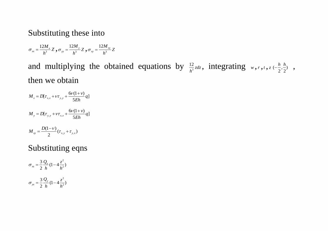
Substituting these into
3
12 xxx
MZ
h ,
3
12 y
yy
MZ
h ,
3
12 xy
xy
MZ
h
and multiplying the obtained equations by 3
12zdz
h, integrating w , r , t , z ( , )
2 2
h h ,
then we obtain
, ,
6 (1 )[ ]
5x x x y y
vM D q
Eh
, ,
6 (1 )[ ]
5y y y x x
vM D q
Eh
, ,
(1 )( )
2xy x y y x
DM
Substituting eqns
2
2
3(1 4 )
2
xxz
Q z
h h
2
2
3(1 4 )
2
y
yz
Q z
h h

Into the 12 xz xz
G
12 yz yz
G
And multiplying the results by
23 2[1 ( ) ]
2
zdz
h h and integrating between
The limits 2
hz , we obtain
, ,
12 1 6
5 5x xx x xw Q w Q
Eh Gh
, ,
12 1 6
5 5y yy y yw Q w Q
Eh Gh
Now eight unknowns, , , , , , ,x y xy x y xM M M Q Q w and y are connected by 2 equations
of (*), 3 equations of (?), and three equations , 0M Q
, 0Q q

Eliminating x , y from above, and taking into account
, 0Q q , we obtain
2 2
, , ,( )5 10 1
xx yyx x x
h qhM D w w Q
2 2
, , ,( )5 10 1
yy xxy y y
h qhM D w w Q
2
, , ,(1 ) ( )10
xyxy x y y x
hM Dw Q Q
Substituting this equation into , 0M Q , we get
2 2 22 ( )
10 10(1 )x x
h w h qQ Q D
x x
2 2 22 ( )
10 10(1 )y y
h w h qQ Q D
y y
To obtain the more complete deflection equation for plate we only have to
substitute the above equations into , 0Q q , we then get 2
4 22
10 1
hD w q q
.
Reissner's theory

Mindlin's theory
Shear deformation 고려(thickness direction)
classical theory
3 shear deformation
33 stretching effect in the thickness direction
3 ,3 3,
1( ) 0
2u u : ,3 3, ,u u w
,3 3,u u ; ,3 3,u u

(constant shear ~)
, ( , )w x y
1st order theory -> higher order theory
, , , ,
1( ) ( )
2 2
zu u
3 3 ,2 w
2
2
( , ) (1, )h
hN M z dz
=>, ,( ) ( )x x y y xD M
, ,( ) ( )y y x x yD M
xyM
z zQ dz kh ; ,( )Q khG w
Shear correction factor steming?? from the fact that z is constant through
the thickness.

Straight line remains straight but conseration?? Of normal discarded.
Meaning of k : surface condition
, 0M Q
, 0Q q ,Q q
, , , ,
1 1[ ] ( ) 0
2 2x xx x yy y xy x xD kGh w
, , , ,
1 1[ ] ( ) 0
2 2y yy y xx x xy y yD kGh w
, , , ,( )xx yy x x y ykGh w w q
Eliminate : 4 2DD w q q
kGh ;verity
5( )
6k

xyM,x yM MConstant bending moments and constant twisting moment . It is
only for convenience that we examine stress states rather than strain states :
typically a computer program outputs stresses rather than strains. Computed
n nodal d.o.f can also be examined; if they are incorrect strains and stresses
will also be incorrect. If displacements are correct but stresses are incorrect,
one suspects that the stress calculation subroutine must be incorrect. Support
conditions must not prevent the constant state from occurring.
............................................................................................................................
................................................................................
~ Effect of locking
1 2
1 2

1 2a a x
1 2b b x
, 1 2 2( )xz x a a x b
2 :xz
1 2 20; 0, 0xz a b a
1 1 1 1,a b a x
2
~ 0bU Lockingx
1 2 1 20, 0xz a b a a x
2 point rule to integrate exactly
reduced integration : 1 point rule

1 1b a x
2 0 ~ 0ba Ux x
Classical(~Thin) plate theory
,0
0 ,
0
( , )( , )( , , )
( , , ) ( , ) ( , )
( , , ) ( , ) 0
x
y
w x yu x yu x y z
v x y z v x y z w x y
w x y z w x y
First-order shear deformation theory
0 1
0 1
0
( , ) ( , )( , , )
( , , ) ( , ) ( , ) :
( , , ) 0( , )
u x y u x yu x y z
v x y z v x y z v x y
w x y z w x y

Shear correction factor : 3 3~ 0 ?
2nd-order(Higher-order)shear deformation theory
0 1 2
2
0 1 2
0
( , ) ( , ) ( , )( , , )
( , , ) ( , ) ( , ) ( , )
( , , ) 0 0( , )
u x y u x y u x yu x y z
v x y z v x y z v x y z v x y
w x y z w x y
Shear correction ?
Generally, n-th order

0 1 2
2
0 1 2
0
( , ) ( , )( , ) ( , )( , , )
( , , ) ( , ) ( , ) ( , ) ...... ( , )
( , , ) 0 0( , ) 0
n
n
n
u x y u x yu x y u x yu x y z
v x y z v x y z v x y z v x y z v x y
w x y z w x y
what is the merit ?
3 33, , : ?
, ,
1( )!
2ij i j j i mi mju u u u

4.3 von Karman Plate theory
The theory of small deflection of thin plate was derived in the previous sections
under the assumption of infinitesimal displacement. For small deflection ( max 0.2w h )
the theory gives sufficiently accurate results. By increasing the magnitude of
deflection beyond a certain level ( max 0.3w h ) however, the lateral deflections are
accompanied by stretching of the middle surface, provided that the edges, or at least
the corners, of the plate are restrained again in-plane motion. Membrane forces
produced by such stretching can help appreciably in carrying the lateral load.
If the plate, for instance, is permitted to deform beyond its thickness,
its load-carrying capacity is already significantly increased.
When maxw h , the membrane action becomes comparable to that of bending.
This is in sharp contrast with the theory of beams, for which the linear theory is valid

as long as the slope of the deflection curve is everywhere small in comparison to
unity.
Figure : Deflection of simply-supported square plate under constant lateral load
A well known theory of large deflection of thin pates is due to von Karman.
In this theory, the following assumptions are made.
~ ( )w O h and w L ; L : typical plate dimension
~The typical displacements ,u v are small, and in the strain-displacement
relations only the quadratic terms in ,xw and , yw are retained.
(or strains are much smaller than rotations)
~Kirchhoff‟s assumption that lines normal to the un-deformed middle surface

remain normal to this surface in the deformed state and are un-extended after
deformation holds.
~The slope is everywhere small, , 1xw and , 1yw .
~All strains are small and Hooke‟s law holds.
Thus von Karman theory differs from the linear theory only in retaining certain
powers of derivatives ,xw and , yw in the strain-displacement relationship. Because of
the Kirchhoff assumption we may write
1
2
3
( , , ) ( , ) ( , ),
( , , ) ( , ) ( , ),
( , , ) ( , )
x
y
u x y z u x y zw x y
u x y z v x y zw x y
u x y z w x y
or
0
3
( , , ) ( , ) ( , ),
( , , ) ( , )
u x y z u x y zw x y
u x y z w x y
% Strain-displacement relation from the theory of elasticity :

, , , ,
1 1( )
2 2ij i j j i k i k je u u u u
3.3.1 Strain – Displacement relationship
,i j ij iju = Stretching + rotation :
Note : 3 12
Model !:
1,2 1,2 2.1 1,2 2,1 12 12
1,3 1,3 3.1 1,3 3,1 13 13
1,1 1,1 1.1 1,1 1,1 11 11 11
1 1( ) ( )
2 2
1 1( ) ( )
2 2
1 1( ) ( ) 0!
2 2
u u u u u
u u u u u
u u u u u

% In the matrix form :
Report : ,[ ] ?i ju
1 1( ) ( )( )
2 2ij ij ij ji ji ki ki kj kje
Symmetric or skew-symmetric part !
1
( )( )2
ij ij ki ki kj kje
2 2
3: ( ), ( ), ( )ijAssume O O O
2 3 3 3 3 3 3 3 4 3 3
3 2 3 3 3 3 33 3 4 3 3 3 33
33 2 33 3 3 3 3 3 3 3 4 3 3 33 33
1 1 1( ) ( ) ( )
2 2 2
1 1( ) ( ) ( )
2 2
1 1 1( ) ( ) ( )
2 2 2
e C C C
e C C C
e C C C

Take
3 3
1
2e
and assuming
3 0 : .( 1 2 : .. )( 3: .. )ie for i or shear deformation i normal deformation
Then
0 1, , , :
2e zw w w
Ex) 0 2 0 2
,
1 1, , , ,
2 2xx xx xx x x xx xe zw w u zw w
...
Q : Non-linear first-order shear deformation theory ? Higher-order shear deformation theory ?

Report : Due Dec.2
Newton-Raphson method, Arch-length method
- Numerical study for nonlinear system - example results
4.2 Equation of equilibrium & Boundary conditions
For a constitutive law, we will employ Hooke‟s laws between the stresses and the
strains for plane stress over the thickness of the plate.
Thus we shall consider here only with ( , 1,2)e .
Accordingly the total potential energy is written by simple form.
At first, the strain energy is written

2
2
h
ij ij
hV
U e dV e dzdA
So, we get
22
11 12 222
2
{ [ ] [.....] [.....]}
h
i
h
u w w wU z dzdA
x x x x
Now we use the notation, 2
2
h
h
M zdz
to get
( What is the difference between linear plate theory ? )
: Couple terms, non-linear terms
22
11 12 222
2
{ [ ] [.....] [.....]}
h
i
h
u w w wU z dzdA
x x x x

2
2{ ( ) ] ..........}i xx xx
u w w wU N M dA
x x x x
~ , , , ,{ ( ) ..........}xx x x x xx xxN u w w M w dA
where
2
2
h
h
N dz
For the applied forces
e s sU q wdxdy N u ds N u ds
where N ; normal force distribution per unit length of the edge which is taken as
positive in compression
sN ; tangential force distribution per unit length of the edge
, su u ; in-plane displacements of the boundary in the directions of normal and

tangential respectively to the boundary. ( , )q x y : ; load distribution (lateral)
By using the above results for iU
and eU we may form U .
Since we used un-deformed states for stresses and external load, we are limited to
small(~moderate) deformation as far as using this approximate functional for the
total potential energy.
Thus we have for the total potential energy principle
0 i eU U U
By using Green‟s Theorem and coordinate transformation from ,x y
to , s and also ,Q M
Then we get

, , , , , , ,
, , , , , , , ,
{( ) ( ) [ 2
( ) ( ) ( ) ( ) ] }
.... .... ] 0
xx x xy y xy x yy y xx xx xy xy yy yy
xx x x yy x y xy y x yy y y
s
N N u N N v M M M
N w N w N w N w q w dxdy
M
~ , , ,3[ ( .?. ) ]
.... .... ] 0s
N u M q u dA
M
Report : Complete „? Portion‟ ( Next week)
The last term accounts for corners in the boundary as was discussed.
From this equation we can conclude that in the interior of the plate
???!!!

The first 2 equations are identical to the equations expressing the equilibrium for
plane stresses. Using these equations to simplify the 3rd equation.
We get
, , 0M N w q
Now comparing this equation with the classical case
, 0M q
We see that it is introduced nonlinear term
(~ , , 2 , , )xx xx xy xy yy yyN w N w N w N w
Involving the in-plane force intensities as additional "transverse loading" terms”
We also obtain the following boundary conditions as the text :
~ or ~ is specified. etc.

The last three conditions are familiar from earlier work on plates. except that the
effective shear force is now argumented by projections of the inplane forces at the
edges.
If we use Hook‟s law to replace the resultant intensity functions by appropriate
derivatives of the displacement field, and carrying out the finite integral w.r.t z, we obtain,
*
2 2
, ,
( , , )
.?.
1 1{[ , ] [ , ]}
2 2
.?..
.. ..
?, ?
xx xx yy
xx x x y y
M D w w M
N C u w v w
can be
M N
where
C : Extensional rigidity

The first two equations will be satisfied if we use a function F defined by
$ , .. , .. ,xx yy xx xx xy xyN F N F N F
Replacing M in terms of ,w and N in terms of derivatives of F above, then the
last equation becomes
Then
4 , , 2 , , , ,yy xx xy xy xx yyD w F w F w F w q
We now have a single partial differential equation with two dependent variables w
and F.
Since we are studying in-plane effects using a stress approach, we must assure the
compatibility of the in-plane displacements. This will give us a second companion
equation to go with the above equation. To do this we have to eliminate ,u v from the

expression on F. It can be done by eliminating ,u v from * and $.
Then the compatibility is given by
4 2( , , , )xx xx yyD F Eh w w w
% Gaussian Curvature
If the surface is developable, the Gaussian curvature vanishes. Hence the right-hand
side of 4 2( , , , )xx xx yyD F Eh w w w vanishes if the deflection surface is developable.
If a flat surface is deformed into a non-developable surface its middle plane will be
stretched in some way and the right-hand side of above equation does not vanish.
Thus, these nonlinear terms arise from the stretching of the middle plane of a flat
plate due to bending into a non-developable surface.
When the nonlinear terms in the above equations are neglected, these equations

reduce to the corresponding equations to the small-deflection theory.
CF) Clamped 4 edges or Cantilever model ?
The first two equations governing the membrane stresses ,xx xy yyN N N are identical
with the linear theory.
Substitution of ~ , ,N u v w into the equations yield the basic equations for
stretching of plate as follows:
, ,) 0 :?xx x xy yex N N ..

3-3-3 Methods of Analysis
(a) Berger‟s Method
2
2 2 2
22
2
122( 1)( , , , ) [ 2( 1) ]
2
: .. var .. .. .. ..
: tan ..
: ..
:
: .. var .. ..
b xx yy xy
xx yy
rr
DU w w w w e e dxdy
h
e First in iant of middle surface strain
rec gular coordinate
cylindrical coordinate
e Second in iant of
2
.. ..
1: tan ..
4
: .. .. .. ..
xx yy xy
rr
middle surface strain
rec gular coordinate
cylindrical coordinate when circular symmetry

% 2
2 2
1, , , : .. ..
2
1 1, , , , , , , , , ,
2 2
rr r r
xx x x yy y y xy y x x y
uu w for symmetric case
r
u w v w u v w w
If the deflection of a plate is of the order of magnitude of its thickness, the
differential equations for the deflection and the displacement can be written in terms
of one fourth order and two second order nonlinear equations. These three equations
are coupled together.
The purpose of the present investigation is to develop a simple and yet sufficiently
accurate method for determining the deflection of plates when that deflection is of
the order of magnitude of the thickness. The approach used in the following analysis
is to investigate the effect of neglecting the strain energy due to the 2nd invariant of
the strains in the middle surface of the plate when deriving the differential equation

by the energy methods. The resulting differential equations are still nonlinear, but
they can be decoupled in such a manner that they may be solved readily.
These equations hereafter will be referred to as the approximate equations. To solve
the problem of large deflections of plates completely, an estimate of the membrane
stresses must be made. This can be done by assuming that the deflection is equal to
that given by the solution to the approximate equations and substituting this
deflection into the strain energy integral. The strain energy is then a function of the
displacements only and, by the principle of virtual displacements, differential
equations can be derived for these displacements..
It is the intent of this investigation to develop a simplified analysis for finding the
deflection of plates when that deflection is large enough so that the strain of the
middle surface cannot be neglected.

H.M. Berger “ A New Approach to the analysis of Large Deflection of Plates”
(b) Banerjee‟s Method
For thin plates undergoing large deflections, a modified energy expressions has been
suggested and a new set of differential equations has been obtained in a decoupled
form. Accuracy of the equations has been tested for a circular and a square plate with
immovable as well as movable edge conditions under a uniform static load. These
new equations are more advantageous than Berger‟s decoupled equations which fail
to give meaningful results for movable edge conditions.
An approximate method for solving the large deflections of plate has been proposed
by Berger. This method is based on the neglect of 2e , the second invariant of the
middle surface strains, in the expression corresponding to the total potential energy
of the system. An advantage of Berger‟s method is that the coupled differential

equations are decoupled if 2e is neglected.
But, some authors pointed out certain inaccuracies in Berger‟s equations and
concluded that Berger‟s line of thought leads to meaningless results for movable
edge conditions. This is due to the fact that the neglect of 2e for movable edges
fails to simply freedom of rotation in the meridian planes where the membrane stress
2
2
1( , , )
1 2rr r r
E uu w
r
exist.
For movable edges the in-plane displacement u is never zero and thus Berger‟s
equations lead to absurd results.

On the other hand, for immovable clamped edge,
0u and 0dw
dr and therefore, Berger‟s equations give sufficiently accurate results.
For simply supported immovable edges, 0u , but 0dw
dr . Thus Berger‟s equations
give fairly accurate result. A modified energy expression has been suggested by
bringing directly the expression for rr in the total potential energy of the system. A
new set of differential equations has been obtained in a decoupled form.
In polar coordinates, the total potential energy, V of a thin isotropic circular plate of
radius a, and of thickness h is given by
2 2 2
, , , , 1 22 20 0
2 1 12[ { 2( 1) }]
2
a a
rr r rr r
D vV w w w w e v e rdr qwrdr
r r n (1)
Where, D is the flexural rigidity of the plate given by 3
212(1 )
EhD
v
, W is deflection, v
is poisson‟s ratio, 1e and 2e the first and second invariant of the middle surface
strains respectively given by

2
1 , ,
1
2r r
ue u w
r
2
2 , ,
1[ ]
2r r
ue u w
r
Here, u is the in-plane displacement and q is the uniform static load. Equation (1)
may be rewritten in the following form
22 2 2 2
, , , , 12 2 20 0
2 1 12[ { (1 ) }]
2
a a
rr r rr r
D v uV w w w w e v rdr qwrdr
r r n r
Where 2
1 , ,
1~
2r r rr
ue u v w
r
If the term 2
2
2(1 )
uv
r in (2) is replaced by
4
4
dw
dr
being a factor depending on the
Poisson‟s ratio for the plate material, decoupling of (2) is possible. Introducing the
term 4
4
dw
dr
in place of 2
2
2(1 )
uv
r
and applying Euler‟s variational method to (2), the following decoupled differential
equation is obtained.

4 1 2 2
, , , ,2 2
12 6( ) ( 2 )rr r r rr
qw w w Ar w w w
h r h D
(3)
Where A is a constant of integration to be determined from 2 1
, ,
1
2
v
r r
uu v w Ar
r
(4)
In the rectangular Cartesion coordinate system (3) is
4 2 2 2 2 2
, , , , , , , ,2 2
12 6( ) [ { } 2{ }]xx yy x y xx x yy y
qw A w vw w w w w w w w
h h D
When the constant of integration A is to be determined from
2 2
, , , ,
1
2 2x y x y
vA u vu w w
To these equations must be added a suitable set of boundary conditions.
Refer to the paper
B.Banerjee& S. Datta “A New Approach to an analysis of Large Deflections of Thin Elastic Plates”