CHAPTER 4

STATISTICS

When we make a measurement several different things may be true:

(1) The parameter we are measuring is random, e.g. flow noise.

(2) The parameter we are trying to measure is deterministic but other parameters affect the

measurement: e.g. environmental factors, electronic noise, quantization noise. Many of

these parameters are random.

The result is our measurement is random, and the result of the next measurement cannot be

predicted exactly. A deterministic measurement is one that can be predicted exactly. So how do

we describe the measurements if they are random? How does the description relate to what we

are trying to measure as opposed to what we do measure? Let's consider the following example

as an illustration of some the things we should be thinking about when we make measurements

of parameters that are random in nature.

EXAMPLE

Suppose we wish to measure the average age of US citizens in Indiana, and we decide to do this

by going into a high school class, asking the ages of the students there and averaging the

answers. It turns out that on this day only 5 students are in class. Let's make some comments

about this.

(a) The Process of Collecting the Data

The average age of students in a high school class is much lower than the average of the US

population. So even if we had thousands of students in our high school class and averaged

their ages, the result would be much less than the US population average age. We say that

there is a "bias" in our estimation procedure. Also the variation of the ages in the high

school class would also be much lower than the variation of ages in the US population. Had

we conducted the test at a location peopled by all age groups we might have wished to take

many samples of people's ages, so that we would feel "happier" that the calculated average

was closer to the true average age of the US population.

(b) The Data

Suppose we wanted to know the average age of students in Grade 11, and the class we

sampled was Grade 11. We would now feel more comfortable that we were collecting a

more appropriate range of samples. However, we only have 5 samples. If we calculated the

average age when more students were in class, the answer would be different, and perhaps

having more sample ages to average we would feel "better" about the calculation.

4-2

In this example we have talked about:

the average value of the data samples,

the spread of the data samples,

the idea that somehow more data is "better",

the idea that the bigger the variation the more desirable it is to take more samples, and

finally,

the idea of bias where you are consistently "off" in your estimates due to some problem

with the way you are calculating what you wish to measure.

In this chapter we will try to formalize these concepts with a mathematical description of the

random data.

DISTRIBUTION OF THE DATA

Suppose we take samples of what we are trying to measure. Let

1 2 NX , X ,…X

be the sample measurements. What is the probability that a measurement (X) is less than a

certain value x? We write this as:

P [X < x].

Based on our sample we would estimate this probability by counting how many Xi are less than

x. Let's denote this by ni, and we estimate the probability that a measurement is less than x by

dividing ni by N. So:

inP [X < x] =

N (1)

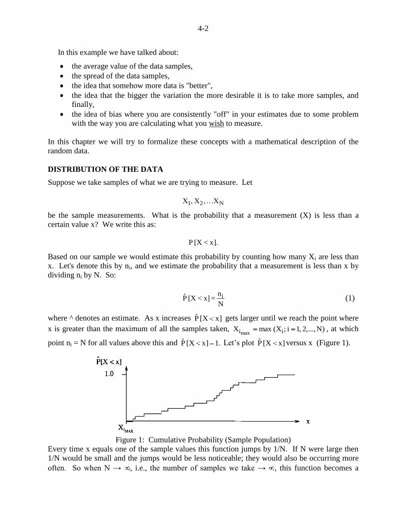
where ^ denotes an estimate. As x increases P [X x] gets larger until we reach the point where

x is greater than the maximum of all the samples taken, maxi iX max (X ; i 1, 2,...,N) , at which

point ni = N for all values above this and P [X x] 1. Let’s plot P [X x] versus x (Figure 1).

Figure 1: Cumulative Probability (Sample Population)

Every time x equals one of the sample values this function jumps by 1/N. If N were large then

1/N would be small and the jumps would be less noticeable; they would also be occurring more

often. So when N → , i.e., the number of samples we take → , this function becomes a

4-3

smooth function of x, as shown below in Figure 2. We refer to the set of all possible samples as

the parent population. When we only have a finite number of samples we refer to this group as a

sample population.

Figure 2: Cumulative Probability (Total Population)

This shape tells us there are not many data values when x < a or when x > b.

In order to show where most data values lie, let's look at the probability of a data value lying

in an interval ∆x, centered on an arbitrary value of x. This is given by:

x x x x

P x X x P X x P X x2 2 2 2

(2)

The result of this calculation is dependent on the interval width ∆x so let's normalize the

calculation by ∆x, and define

x xP X x P X x

2 2p(x)

x (3)

Now let ∆x 0 and then

x o

dˆp(x) lim p(x) P[X x].

dx (4)

If we differentiate the function, P[X < x] shown in Figure 2, we should have a function similar to

the p(x) shown in Figure 3.

p(x)

x

a c b

Figure 3: Probability density function

4-4

p(x) is called the probability density function and shows us where the data values are most likely

to occur. From Figure 3 we can see that many of the data samples will have values near x = c.

There are many different types of probability density functions. Here are two examples.

(a) GAUSSIAN OR NORMAL PROBABILITY DENSITY FUNCTION

p(x)

2x2

x

1(x )

2

x

1p(x) e

2 (5)

x

Figure 4: Gaussian probability density function

Many noise signals approximately have this distribution. Also, if a measurement is the outcome

of many random events, the distribution will tend to be Gaussian. We see that values of x close

to x

are more like to occur than other values.

(b) UNIFORM PROBABILITY DENSITY FUNCTION

p(x)

1 p(x) = 1

2B , A – B < x < A + B (6)

2B

= 0 , elsewhere.

x

A-B A A+B

Figure 5

Calculating the Probability that X Lies in an Interval, a < X < b by using p(x)

Since p(x) is the derivative of P[X < x], then the probability that X lies between a and b is

integral of p(x) between a and b, given by:

b

a

P[a X b] p(x) dx. (7)

Figure 6: Rayleigh distribution

21x

2rx

p(x) e .r

4-5

This is illustrated in Figure 6 where the probability density function (pdf) of a Rayleigh

distributed random variable is shown.

Note that a property of ALL probability density functions is:

p(x) dx 1, (8)

which is to say that the probability that X takes a value between - and + is 1.

EXAMPLE

If p(x) is the pdf of a uniformly distributed random variable, such

p(x) = 12 10 < x < Q

= 0 x < 10 , x > Q.

Calculate Q.

Solution p(x)

12 The total area under the probability density function

should equal one.

x Area = (Q – 10) 12 = 1.

10 Q

Therefore Q = 10 1/12.

Figure 7: Uniform distribution

EXAMPLE

If the pdf of a random variable, X, is

2x

B1p(x) e

A, what is the relationship between A and B?

Solution

This looks like a Gaussian distributed random variable where p(x) has the form:

2x2

x

1(x )

2

x

1p(x) e

2

Setting 2x x

x

0 ; 2 B and 2 A, we derive the relationship:

2A

B2 2

xA 2 B ,

EXAMPLE

4-6

The pdf of a random variable (x) is

2x

2rxp(x) e

r for x > 0, and p(x) = 0 for x < 0.

What is the probability of X lying between 10 and 25?

Solution 2

2x

25 25x / 2r2r

10 10

x dP[10 x 25] e dx e dx

r dx

Note 2 2x / 2r x /2rd x

e edx r

so,

2 25x /2r 100/ 2r 625/ 2r

10

P[10 x 25] e e e

MOMENTS OF THE DATA e.g. mean, variance etc.

In this section we will describe calculation of moments of a random variable, e.g., mean value,

mean square value, etc.

Mean Value

If we wished to estimate the average or mean of our data samples we would calculate

N

ii 1

1X

N ,

If we know p(x) how can we calculate the mean value? Consider a small interval centered on

cx of width x, as shown in Figure 8(a).

Shaded area is c cx x

P[x x x ]2 2

Normalized histogram of the data =

icn /(N x).

Let's start with calculating how many of the total number of samples, N, fall into this interval:

4-7

c cx x

x X x .2 2

The number of values in this interval, cn , is the total number of values (N) times the probability

of a value lying in the interval, which is:

c

c

x x/2c c c x x/2

x Xn N P x X x N p(x) dx

2 2 (9)

If x is small, this tells us how many values we have approximately equal to cx . Splitting the

full range of data into bins x wide, centered on icx , we can replace p(x) by an approximate

histogram representation (Figure 8(b)). We can then say that we have approximately 1cn values

equal to 1cx ,

2cn values equal to 2cx and so on. The average can then be estimated by using:

ci i1 1 2 2 M M i ici

M M x x / 2cc c c c c c c cx x / 2

i 1 i 1

n1n x n x n x x p(x) x dx

N N (10)

Letting x 0 the bins become smaller and the icx become closer until they join up and become

continuous: icx 0 and c x /2i

c x /2i

M x

xi 1

. Therefore the mean, which we denote by x

is

given by:

x

Average or mean or E[X] x p(x)dx . (11)

The E[.] denotes expected value of, or average value of whatever is inside the brackets.

EXAMPLE

A random variable, X, has a probability density function p(x) = 0 when x < 0, p(x) = x when

0 < x < B, and p(x) = 0 when x > B. Calculate the mean value of X.

Solution

Lets denote the mean value of X by .

B

3

0

1E[X] x x dx B

3.

Because we know that the total area under the p.d.f. is 1, we can also calculate .

B

2

0

11 x dx B

2.

4-8

Hence 2

2 2, and B

3B.

Mean Value of a Function of a Random Variable

Using similar arguments to the derivation of the formula for calculating the mean, it is possible

to show the following. If Y is a function of a random variable X, Y = g(X), and X has a

probability density function p(x), then the mean value of Y is given by:

E[Y] E[g(X)] g(x)p(x)dx. (12)

EXAMPLE

Suppose that nRT

PV

and n, R and T are constant but V is a uniformly distributed random

variable with a p.d.f., p(V) = 1

Bfor V in the range o o

B BV V V

2 2, and p(V) = 0 outside this

range. Note that, because the V has a uniform distribution, the mean value of V is oV , the center

value of the range of values that V can take. Calculate the mean value of P.

Solution

o o

o o

B BV V

2 2

pB B

V V2 2

nRT nRT nRT 1E[P] E p(V) dV dV

V V V B

enRT

log (V)B

o

oe

o

o

BV

2nRT V B/2

logB V B/2

BV

2

.

You might note here that:

pnRT

E[V] which would equal

o

nrT

V.

However, if B is small, it can be shown, by expanding the log function in a Taylor series

expansion, that

p is approximately equal o

nRT

V .

4-9

Later in the propagation of error section we will make this assumption. Remember when you

use it, that it is based on the assumption that the variation is small which may not, in general, be

true. You actually knew this, if you thought about it. For example, consider Y = X2, with X

uniformly distributed in the interval -3 < X < +3. Y will take values in the interval 0 < Y < 9 and

is not uniformly distributed. The mean of X is 0, the mean of Y is obviously not the mean of X

squared, i.e., 2x , which is 0. In fact, the mean of Y is 3. Using equation (12), prove this as an

exercise.

Variance and Standard Deviation

To measure the spread of the data we look at how the data varies about its mean value, . If we

have our N samples, and say we know the mean, we measure the variation in the data with the

following estimate,

N

2i

i 1

1(X )

N . (13)

If we know p(x) we can calculate this exactly. This quantity is called the variance, which we

denote by 2x , and using equation (12), where the function is 2(x ) , we can show that:

2 2 2x E[(X ) ] (x ) p(x)dx (14)

The standard deviation, x , is the square root of the variance.

EXAMPLE

Show that the mean value of a random variable with the following Gaussian distribution is c.

21(x c)

21p(x) e

2

Solution

21(x c)

2

x

1E[X] xp(x)dx xe dx

2

2 21 1(x c) (x c)

2 21 1(x c)e dx c e dx

2 2

21(x c)

21e

2 c. p(x)dx 0.0 c.1 c. .

4-10

As x , 21

(x c)2e 0. Therefore the first term is zero. By definition the integral of p(x)

over the entire range of possible values for x is 1; the second term is therefore equal to c, giving

the required result.

EXAMPLE

Calculate the variance of a random variable with the following uniform distribution.

p( )

1p( ) for , p( ) 0,

2 elsewhere.

-x 0 x

Solution

2 2E[( ) ] ; 0 from inspection. 2 2 2E[ ] p( )d

3

21d

2 6

3 2

.3 3

EXAMPLE

Y = 3X2 – 12 and X is a random variable with a uniform distribution:

p(x) 1/2 for x , and 0, elsewhere.

What is the standard deviation of Y?

Solution

Let's first calculate the variance of Y.

2 2 22 2 2 2 2y

y y y y y y

E[(Y ) ] E[(Y 2Y ] E[Y ] 2E[Y] E[Y ]

2 2

y y

E[Y] 3E[X ] 12 12

Note we used 2

2E[X ] ,3

which we calculated in the previous example.

E[Y2] = E[9 X

4 – 72 X

2 + 144] = 9E[X

4] – 72E[X

2] + 144

1

2

4-11

E[X4] =

541 x

x dx2 10

4

5

4 2 4

2 2 2 2 2 4 2 2 4y

y

9 9 4E[Y ] 72 144 ( 12) 24 24

5 3 5 5.

The standard deviation of Y is y , that is, the square root of the variance. Hence,

2y

2

5.

ESTIMATES OF MEAN AND STANDARD DEVIATION

Most often we do not know p(x) and must estimate xx

and from the sample data values. The

formulas we use are:

N

ii 1x

1ˆX or X

N,

(15)

2N N

2 2 2x x i i

i 1 i 1x

1 1ˆand s or X or (X X)

N (N 1). (16)

Note that we have introduced some new notation. ^ is used to denote an estimate of a

quantity and hence x

ˆ denotes and estimate of the mean of X. The notation X is often used in

texts to denote the same thing, and is included here so that you become familiar with both

notations. In different texts you will find a wide variety of notation, so take care when reading to

understand that particular author's notation. Following our ^ notation 2xˆ , denotes an estimate of

the variance; another commonly used notation for this estimate is 2xs .

Each time we measure N samples and calculate xX and s we get a different answer.

xX and s are themselves random variables. In this section we will look at the properties of X and

how they are related to the properties of X, the data samples.

If X1, X2….Xn are independent measurements then we may write, if i j, that

i j i j

i j i jx x x x

E[(X ) (X )] E[(X )] E[(X )].

If i = j, then we have

4-12

ii

2 2i x

x

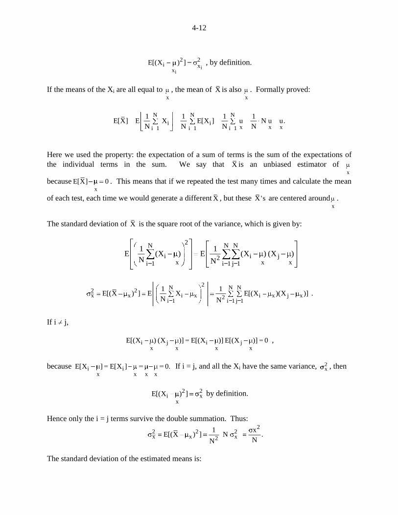
E[(X ) ] , by definition.

If the means of the Xi are all equal to x

, the mean of X is also x

. Formally proved:

N N N

i ix x xi 1 i 1 i 1

1 1 1 1E[X] E X E[X ] u N u u.

N N N N

Here we used the property: the expectation of a sum of terms is the sum of the expectations of

the individual terms in the sum. We say that X is an unbiased estimator of x

becausex

E[X] 0 . This means that if we repeated the test many times and calculate the mean

of each test, each time we would generate a different X , but these X's are centered aroundx

.

The standard deviation of X is the square root of the variance, which is given by:

2N N N

i i j2x x xi 1 i 1 j 1

1 1E (X ) E (X ) (X )

N N

2

N N N2 2x x i x i x j x2

i 1 i 1 j 1

1 1E[(X ) ] E X E[(X )(X )]

N N .

If i j,

i j i jx x x x

E[(X ) (X )] E[(X )] E[(X )] 0 ,

because i ix x x x

E[X ] E[X ] 0. If i = j, and all the Xi have the same variance, 2x , then

2 2

i xx

E[(X ) ] by definition.

Hence only the i = j terms survive the double summation. Thus:

2

2 2 2x x x2

1 xE[(X ) ] N .

NN

The standard deviation of the estimated means is:

4-13

2

2 x xx x .

N N (17)

This is an example of a case where you can see that more data (larger N) will lead to lower

variance of the estimated mean, and hence the estimate of the mean is improved by taking more

data.

What is p(x) , the pdf for X ? How does it relate to p(x)? If p(x) is Gaussian distributed and

N is large (in excess of 60) then p (x) is also approximately Gaussian with mean x

and standard

deviation, xx 1/ 2N

. The two distributions are shown together in Figure 9, for N = 100.

Figure 9: The probability density function of the data and of the estimated mean of the data

CONFIDENCE INTERVALS BASED ON X

Having taken N measurements and calculated X , we can derive the distribution of X if we

assume that X is a Gaussian distributed random variable. (For N large, X will have a Gaussian

distribution, for N < 60 it will have a student-T distribution). Consider the case where N is large

and

2 22 2

x xx x

1 N(x ) (x )

2 2

x x

1 Np(x) e e

2 2. (18)

This is illustrated in Figure 10. The total area of the shaded regions in this figure is .32. So if

the estimation of the mean were repeated many times, 68% of the estimated mean values would

lie in the region

xx

.

4-14

We might say that

x xx x

P[ X ] 0.68 .

Rearranging the inequality we say, we are 68% confident that the true mean x

( ) lies in the

interval:

x xx

X X .

This is a 68% confidence interval.

Figure 10: The probability density function of the estimated mean, X .

To be more confident that the true value lies in a particular interval then we need to widen

that interval. In general, if

Q xx

Q xx

z

z

p(X) dX Q

then the 100 Q% confidence interval for x

is

Q x Q xx

X z X z (19)

Qz can be taken from look-up tables (see Appendix A of this Chapter). x is not known but is

estimated by using:

x xx 1/ 2 1/ 2

s

N N.

EXAMPLE

p(x)

4-15

400 measurements of temperature are taken. X was calculated as 85.6 F and xs was calculated

as 5.3 F. What is the 95% confidence interval for the temperature?

Solution The 95% confidence interval is, approximately,

.95 xX z s .

xx 1/ 2

s 5.3s .265 F

20N

From look-up tables z.95 = 1.96. Therefore the 95% confidence interval is

85.6 1.96 .265 F .

Calculating confidence intervals for the true mean when N < 60

When less than 60 data values are available we may no longer use the Qz values derived from

assuming that X has a Gaussian distribution. In these cases we choose values taken from a

student-T distribution; this distribution is a function of the number of data samples, N. Again we

use look-up tables to determine these values (see Appendix B of this chapter). So for N < 60 the

100Q% confidence interval is approximately:

,Q xX t s , where N 1 (20)

EXAMPLE

25 measurements of pressure are taken, and the mean and standard deviation calculated:

X 201.3 p.s.i. and xs 3.5 p.s.i.

Calculate the 99% confidence interval for the true value.

How many more measurements need to be made so that the 99% confidence interval is

X .005 p.s.i?

Solution

xx 1/ 2

s 3.5s 0.7

5N p.s.i.

99% confidence interval is

24,99 xX t s 201.3 2.775 0.7 p.s.i.

The 0.005 p.s.i. is so small that we will assume that the number of measurements necessary will

be in excess of 100. Therefore

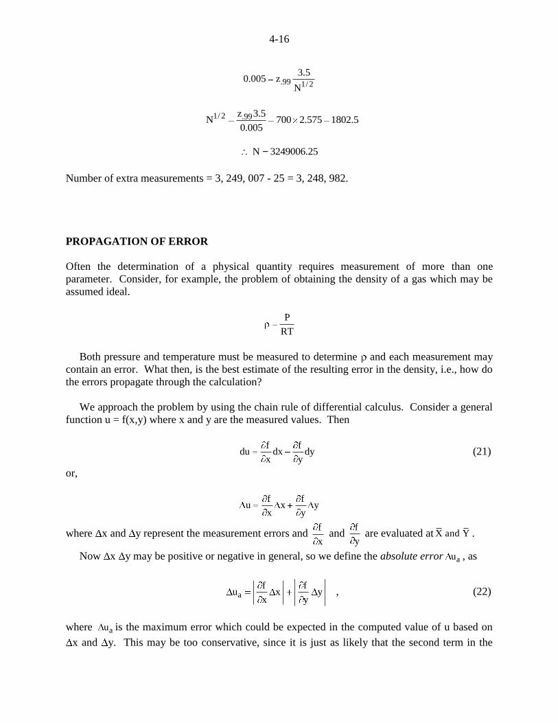
4-16

.99 1/ 2

3.50.005 z

N

1/ 2 .99z 3.5N 700 2.575 1802.5

0.005

N 3249006.25

Number of extra measurements = 3, 249, 007 - 25 = 3, 248, 982.

PROPAGATION OF ERROR

Often the determination of a physical quantity requires measurement of more than one

parameter. Consider, for example, the problem of obtaining the density of a gas which may be

assumed ideal.

P

RT

Both pressure and temperature must be measured to determine and each measurement may

contain an error. What then, is the best estimate of the resulting error in the density, i.e., how do

the errors propagate through the calculation?

We approach the problem by using the chain rule of differential calculus. Consider a general

function u = f(x,y) where x and y are the measured values. Then

f f

du dx dyx y

(21)

or,

f fu x y

x y

where x and y represent the measurement errors and f

x and

f

y are evaluated at X and Y .

Now x y may be positive or negative in general, so we define the absolute error au , as

af f

u x yx y

, (22)

where au is the maximum error which could be expected in the computed value of u based on

x and y. This may be too conservative, since it is just as likely that the second term in the

4-17

above equation could subtract from the first as add. Therefore another commonly used error

estimate is ru :

22

rf f

u x yx y

(23)

In general, then, the value of u would be reported in terms of a 100Q% confidence interval of the

form:

u u u

where u is chosen to be ru , and the 100Q% confidence intervals for X and Y were X x and

Y y , respectively. We approximate u by f (X, Y) , which is an approximation that is true

only if X and Y are small, as discussed earlier.

We have limited our discussion to functions of only two independent variables. However, the

extension to functions of three or more variables is straightforward. As the number of

independent variables increases ru rather than au becomes a better estimate of the error, since

the probability that all errors will be additive decreases. If

1 2 NY f (X ,X , ,X )

and we have calculated 100Q% confidence intervals for i i iX : X x . The 100Q% confidence

interval for Y is Y y where:

1 2 3 NY f (X ,X ,X X ) and

2N

ii 1 i

1 1 2 2

fy x

Xx x ,x x

(24)

EXAMPLE

As an example of the above procedure consider again the gas density measurement problem.

The basic equation is

P

RT

Assume R is known exactly and confidence intervals for P and T are P P and T T

respectively.

2

1 Pand

P RT T RT

The absolute error in is then

4-18

a 2

1 PP T

RT RT

and

22

2r 2

1 PP T

RT RT

With these equations, and estimates of the resolution of available instrumentation for measuring

pressure and temperature, one can readily determine if a is dominated by the expected error in

P or T . Steps can then be taken to improve the instrumentation for one or both measurements to

achieve a desired error bound in the measured density. One of the advantages of this analysis is

that it can provide such information before any data is actually taken, thus saving time and

money.

FITTING FUNCTIONS TO DATA

When we do static calibration we are often interested in fitting a model: f(x), to the input-

output data: i i(X ,Y ) . Let's assume for simplicity that the iX are exact but the iY deviate from the

model. So

i i iY f (X ) n (25)

where ni is the error in the ith measurement, or the amount the ith measurement deviates from the

data model.

There are many ways that we can optimize the choice of the function parameters, given the

data: i i(X ,Y ), i = 1, 2....N. For example, one is called Maximum Likelihood Estimation and

another is called Least Squares Estimation. If we assume that the ni are independent, Gaussian

distributed random variables, both approaches lead to the same set of equations. We will briefly

outline the least squares approach here.

Least Squares Estimation

In this approach we compose a function that measures the cost of getting the model wrong. This

is called the cost function. Here we will just use a measure of the total squared error at each data

point as our cost function. Sometimes, for example in controls, people add other terms to the

cost function such as how much power is being used to actuate a system to achieve the desired

output. In this way we ensure that the optimum solution is one that does not take too much

power to achieve, and so there will be a trade-off between power consumption and accuracy.

However, if we just use the squared error the cost function will look like:

4-19

N N 22

o 1 i i i o 1i 1 i 1

J(a ,a , ) n Y f (X ,a ,a , ) . (26)

We now minimize this cost function J by our choice of the parameters in the model: o 1a ,a , .

To do this we differentiate equation (26) with respect to ai , i = 0, 1, 2,...... and set the results to

zero. This will give us a set of equations to solve for the parameter estimates. If the function that

we are fitting to the data is a straight line: f(x) = ao + a1x, then the equations we need to solve

are:

N

i o 1 ii 1

ˆ ˆ0 2(Y a a X ) ( 1) (27a)

and

N

i o 1 i ii 1

ˆ ˆ0 2(Y a a X ) ( X ) . (27b)

Note that we have replaced a0 and a1 by 0 1ˆ ˆa and a , respectively. This is because the result that

you get is dependent on the data set that you collected. Even if the number of data points (N) is

large, each time the experiment is repeated and a new set of (Xi , Yi) are taken, the estimate will

be slightly different.

For simplicity, we will now stop explicitly including the limits on the summations.

Rearranging equations (27) gives:

, i o 1 iˆ ˆY a N a X (28a)

and

, 2i i o i 1 iˆ ˆX Y a X a X (28b)

or in matrix form:

ii 0

2i i 1i i

N , X ˆY a

ˆX Y aX , X. (29)

These are called the normal equations.

We could also have derived these equations by using vector notation. Starting with equation

(25) and writing it down using this straight line model for i = 1, 2,...N, we can generate a set of

equations. This set of equations can be written in matrix form:

4-20

1 1 1

2 2 20

1

N N N

Y 1, X n

Y 1, X na

, a

Y 1, X n

, (30a)

which can be written even more simply as:

y A a n (30b)

The cost function can now be written as:

T T T T T T TJ n . n y A a a A y y y a A A a. (31)

If you minimize this set of equations with respect to the parameters in a, then you will get the set

of normal equations:

T T ˆA y A A a, (32)

which you can show are identical to equations (29).

Equation (32) could be thought of as the result of pre-multiplying equation (30b) AT,

removing the AT n term and replacing a by a . The solution to these equations is:

i i i i1

N X Y X Ya , (33a)

and

2

i i i i i0

Y X X X Ya , (33b)

where

2 2i idet N (X ) ( X )TA A . (33c)

Thus, equations (33a-c) can be used to determine the gradient and intercept of the best

straight line fit to the data.

Standard Deviation of ˆ ˆi 0 1n , a and a .

Recalling that Yi = f(Xi) + ni and that the Xi are known exactly, then the standard deviation of

Yi once the relationship to Xi is removed is equal to the standard deviation of ni. That is:

i i iy f (x ) n n . We will retain the subscript n to remind ourselves that it is the standard

deviation of the error between the model and the data.

4-21

The easiest way to look at the variance of the parameter estimates is to look at:

1 1 2 1T T T T T Tnˆ ˆE[(a a).(a a) ] E[[A A] A n.n A[A A] ] [A A] . (34)

This result comes from assuming that the errors (ni) are independent. That is, the error at one

data point does not have a functional relationship to the error at another data point. The diagonal

elements of this covariance matrix give the variance of the parameters. Using equations (29) and

(32) and your linear algebra knowledge gives:

2i i

Ti

X , X

X , Ndet [A A]

T -1 1[A A] .

Therefore pulling off the diagonal elements of this matrix, recalling that Tdet[A A] and

scaling by 2n as shown in equation (34), gives:

1 0

22 22 2n

ˆ ˆa n a iN

, X . (35)

We can estimate 2n by estimating the variance of the noise that is the difference between the

model prediction of Yi and the measured Yi. The formula is:

N N

2 2 2n i i 0 1 i

i 1 i 1

1 1ˆ ˆˆ (n ) (Y a a X )

N 2 N 2. (36)

Note that there is an (N-2) in the denominator. In order to calculate this we needed to estimate

a0 and a1 from the data. Since the data has been used to estimate two of the parameters used in

this formula, we have to subtract two from the N. It can be shown formally that this yields an

unbiased estimate of 2n .

You need to be very careful about notation here, because the mean value of Y varies with X.

Subtract f(Xi) from Yi and then calculate 2nˆ ; this is really a measure of the variance of Y and

thus is sometimes denoted by 2y . However, in other texts 2

nˆ is denoted by 2yxs , which one

could term the variance of y once the functional relationship with x has been removed. More

usually 2y is defined as:

N

2 2 2 2 2y y y i

i 1y

1ˆE[(Y ) ], or s (Y Y)

N 1 , (37)

i.e. calculated ignoring the functional relationship between X and Y. The moral is: you need to

understand the notation in the text you are using - not all texts use the same notation and not all

4-22

notation makes that much sense! We will use equation (37) as the definition of 2y , the variance

of Y.

Confidence Intervals for the Parameter Estimates.

Now that we can calculate estimates (equations (33)) and the standard deviation of the

estimates,0aˆ and

1aˆ , (equations (35)), we are in a position to write down the confidence

intervals for the parameter estimates. For N < 60, the distribution that is used to construct the

confidence interval scaling, ,100Qt , has N-2 degrees of freedom, i.e., N 2 . So the 100Q%

confidence interval is:

iˆi N 2,100Q aˆ ˆa t for N < 60; (38a)

or iˆi Q aˆ ˆa z for N 60 , (38b)

where the subscript i is either 0 (bias estimate) or 1 (sensitivity estimate).

How well does the model fit the data?

A measure of how well the model fits the data is given by

Adjusted 2

2 n2y

ˆR 1

ˆ (39a)

Unadjusted 2

2 n2

i y

ˆSum of squares of error (N 2)R 1 1

Sum of squares of (Y Y) ˆ(N 1) , (39b)

which is the fraction of the output data variation that is explained by the model. 2nˆ is calculated

by using equation (36) and 2yˆ is calculated by using equation (37). Here R

2 =1 implies a perfect

fit to the data. R2 = 0.5 may imply a poor fit to the data. What is poor depends on what you are

measuring. For most measurements we do in this course, 0.5 would imply a poor model. If you

were measuring something that has inherently high variability, e.g., a person's response to music

(like/dislike), and relating it to sound level, a value of 0.5 might imply a reasonably good model.

Too few data points (N) compared to the number of parameters (NP)

How large does N need to be? The answer to this is really determined by the level of noise. If

there is a lot of noise on the data, you will need a lot of data to cancel out the effects of the noise

and to make the variances of the estimates small. While it is not obvious from the formulae,

there is a (1/N) factor in equations (35) because in the denominator ( ) the terms arise from

4-23

products of two summations, and in the numerator the terms arise from single summations. This

1/N factor means that the variance decreases with the number of data points used in the

estimation.

If there are too few data points (N is not much bigger than NP), the R2 value can be close to

one. For example, if you are fitting a straight line to two data points R2 = 1.0 because there is

apparently no error, the line goes through the data points. So you might think that this is the

perfect model. However, if you took another two data points and fit a line through them the

answer would be different if the ni are not zero, and yet R2 still equals 1. People often say that

the model is adapting to or fitting the noise in the data set. To avoid this problem you need to

have the number of data points to be at least 4-10 times the number of parameters, and, in

general, even more data is better.

A very high R2 value is suspicious. You should repeat the test to see if your parameter

estimates change significantly with the new set of data. If they do, you are probably modeling the

noise in your data set. If they change little, then perhaps you do really have a good model!

Another indicator of this problem is when the adjusted and unadjusted R2 values are very

different.

If R2 is small, you could still have a good model of the underlying functional relationship

between the Xi and the Yi. This would be the case if, the model structure (straight line) was

correct, there was a lot of noise on the measurements, but you used many measurements when

making the estimates of the parameters of the model (N very large). In this case the 2nˆ will be

large because of the high level of noise, and as a consequence R2 will be small.

So the bottom line is: R2 is a measure of how well your model fits the data set you have.

It is not a measure of how good your model is. However, when used carefully, R2 calculations

may be useful in helping you determine if your model is good.

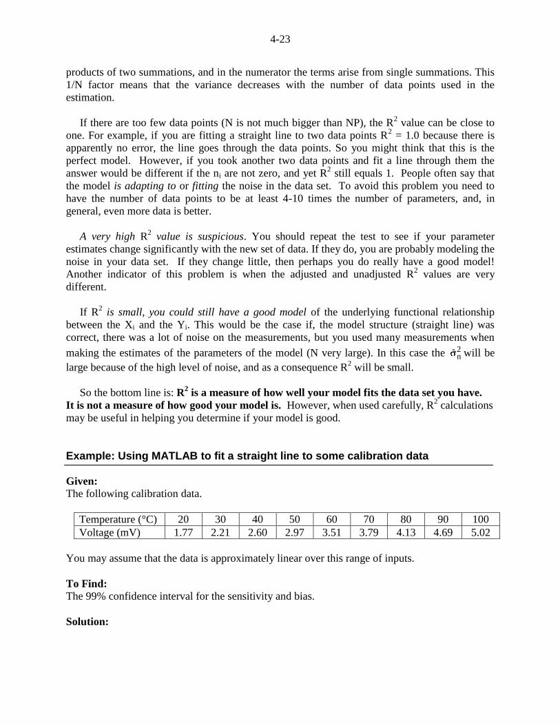
Example: Using MATLAB to fit a straight line to some calibration data

Given:

The following calibration data.

Temperature (°C) 20 30 40 50 60 70 80 90 100

Voltage (mV) 1.77 2.21 2.60 2.97 3.51 3.79 4.13 4.69 5.02

You may assume that the data is approximately linear over this range of inputs.

To Find:

The 99% confidence interval for the sensitivity and bias.

Solution:

4-24

An m-file was written to do the calculation using regress and also by explicitly doing the

calculations after first calculating the vector and matrix in the normal equations (29). The m-file

is listed below, after the output it generates.

M-file Output

ans =

Regress results

biasCI =

0.9780 +- 0.1760 mV

SensitivityCI =

0.0405 +- 0.0027 mV/degC

R2 =

Coefficient of determination: 0.9975

ans =

Own analysis results

biasCI =

0.9780 +- 0.1760 mV

SensitivityCI =

0.0405 +- 0.0027 mV/degC

R2 =

Unadjusted coefficient of determination: 0.9975

R2 =

Adjusted coefficient of determination: 0.9971

It appears that the R2 calculation that MATLAB does is the unadjusted R2 value.

M-file listing

% exreg.m program to fit a straight line through

% static calibration from a thermocouple.

%

temp=(20:10:100)';

N=length(temp);

y=[1.77 2.21 2.60 2.97 3.51 3.79 4.13 4.69 5.02]';

%

% Now do straight line fit using regress and construct the

% 99% confidence intervals.

[a,aint,r,rint,stats] = regress(y,[ones(size(temp)),temp],0.01);

%

% Calculate the uncertainty in the estimates:

% From the calculated confidence intervals.

Da=(aint(:,2)-aint(:,1))/2;

%

sprintf('\\n Regress results ')

biasCI = sprintf('%4.4f +- %4.4f mV',a(1), Da(1))

SensitivityCI = sprintf('%4.4f +- %4.4f mV/degC',a(2), Da(2))

R2 = sprintf('Coefficient of determination: %4.4f ',stats(1))

%

%-------------------------------------------------------------

% now do it by programming the normal equations yourself

% ATy = ATA a

%

4-25

ATA(1,1)=N;

ATA(1,2)=sum(temp);

ATA(2,1)=ATA(1,2);

ATA(2,2)=sum(temp.*temp);

ATy(1)=sum(y);

ATy(2)=sum(temp.*y);

%

%Solve equations: See equations (33) in Notes, Chapter 4

Del = ATA(1,1)*ATA(2,2)-ATA(1,2)*ATA(2,1);

a(1) = (ATA(2,2)*ATy(1)- ATA(2,1)*ATy(2))/Del;

a(2) = (ATA(1,1)*ATy(2)- ATA(1,2)*ATy(1))/Del;

%

% Work out what the noise is, and its variance:

ypred=a(1)+a(2)*temp;

noise=y-ypred;

varn=sum(noise.^2)/(N-2);

%

% Now work out confidence interval

% We use the T-distribution tables, but with

% nu = N-2 = 9-2 = 7

%

tnu_99=3.499;

Da= tnu_99*sqrt(varn*[ATA(2,2);ATA(1,1)]/Del);

%

sprintf('\\n Own analysis results ')

biasCI = sprintf('%4.4f +- %4.4f mV',a(1), Da(1))

SensitivityCI = sprintf('%4.4f +- %4.4f mV/degC',a(2), Da(2))

%

% Now calculate the variance of y for the R^2 calculation.

vary=(1/(N-1))*sum( (y-mean(y)).^2 );

%

% Calculate the unadjusted R^2 and adjusted R^2 value

% Unadjusted is based on sum of squares, Adjusted on estimated

% variances.

sta = 1 - (((N-2)*varn)/((N-1)*vary));

stats(1) = 1.0 - varn/vary;

R2 = sprintf('Unadjusted coefficient of determination: %4.4f ' , sta)

R2 = sprintf('Adjusted coefficient of determination: %4.4f ' , stats(1))

Example: Using MATLAB to fit a quadratic function to some calibration data

Given:

The following calibration data.

Temperature ( C) 20 30 40 50 60 70 80 90 100

Voltage (mV) 1.77 2.21 2.60 2.97 3.51 3.79 4.13 4.69 5.02

Find:

A quadratic function that fits this data.

Solution:

Following is the output of MATLAB program listed below. In contrast to the above example, I

have used MATLAB's own linear equation solver.

4-26

M-file Output

ans =

Regress results

b0_CI =

0.9609 +- 0.4461 mV

b1_CI =

0.0412 +- 0.0166 mV/degC

b2_CI =

-0.000006 +- 0.000136 mV/(degC*degC)

R2 =

Coefficient of determination: 0.9975

ans =

Own analysis results

b0_CI =

0.9609 +- 0.4461 mV

b1_CI =

0.0412 +- 0.0166 mV/degC

b2_CI =

-0.000006 +- 0.000136 mV/(degC*degC)

R2 =

Unadjusted coefficient of determination: 0.9975

R2 =

Adjusted coefficient of determination: 0.9967

Note that the coefficient of the squared term is effectively zero, showing us that this model has

no advantage over a linear model. Also, if you compare the 2R value in this example with that

calculated with the linear model, shown in the previous example, the value has not really

changed at all.

M-file Listing

% exreg2.m program to fit a quadratic to calibration data.

%

temp=(20:10:100)';

N=length(temp);

y=[1.77 2.21 2.60 2.97 3.51 3.79 4.13 4.69 5.02]';

%

% Now do quadratic fit using regress and construct the

% 99% confidence intervals.

A=[ones(size(temp)),temp,temp.*temp];

[b,bint,r,rint,stats] = regress(y,A,0.01);

%

% Calculate the uncertainty in the estimates:

% From the calculated confidence intervals.

Da=(bint(:,2)-bint(:,1))/2;

%

sprintf('\\n Regress results ')

b0_CI = sprintf('%4.4f +- %4.4f mV', b(1), Da(1))

b1_CI = sprintf('%4.4f +- %4.4f mV/degC', b(2), Da(2))

b2_CI = sprintf('%4.6f +- %4.6f mV/(degC*degC)', b(3), Da(3))

4-27

R2 = sprintf('Coefficient of determination: %4.4f ', stats(1))

%

%_____________________________________________________________

% Now do it via the normal equations.

% For ease of notation set Q = AtA and p=Aty

%

A=[ones(size(temp)),temp,temp.*temp];

Q=A'*A; p=A'*y;

%

% Solve the set of linear normal equations: p = Q b

b=Q\\p;

% This should give the same results as:

b1=A\\y;

% because MATLAB solves y = A b1 using least squares.

%

% Find the error (noise) vector and its variance

no=y-A*b;

varn=(sum(no.*no))/(N-3);

%

% Find the variance of Y

vary=sum((y-mean(y)).^2)/(N-1);

%

%Find the diagonal elements of Q inverse and scale by variance of

%noise (varn) to find variance of estimates.

varb=diag(inv(Q))*varn;

%

% Scale by t(N-3,100Q)=t(6,99) to generate confidence interval.

t6_99=3.707;

Da=sqrt(varb)*t6_99;

%

%Now calculate the R^2 value

stats(1)=1-(((N-3)*varn)/((N-1)*vary));

sta=1-(varn/vary);

%

% Now print out the results

sprintf('\\n Own analysis results ')

b0_CI = sprintf('%4.4f +- %4.4f mV',b(1), Da(1))

b1_CI = sprintf('%4.4f +- %4.4f mV/degC',b(2), Da(2))

b2_CI = sprintf('%4.6f +- %4.6f mV/(degC*degC)' ,b(3),Da(3))

R2 = sprintf('Unadjusted coefficient of determination: %4.4f ' ,stats(1))

R2 = sprintf('Adjusted coefficient of determination: %4.4f ' ,sta)

Differentiating Between Repeatability and Nonlinearity.

When the variation in data is large it is difficult to determine whether the deviations from a

straight line that you observe are due to nonlinearity or due to random variability (noise). To

distinguish between the two we need to reduce the random variation in the data until it is small

when compared to the variation due to the nonlinearity. We do this by repeating the test and

averaging. For each input value we can calculate the mean and the standard deviation of a set of

nominally identical measurements, and then we can estimate confidence intervals (68% or 95%

or 99%) for the true mean at each input value. This is illustrated in Figures 11a and 11b. The

standard deviation of the data can be used as a measure of the repeatability of the measurements.

4-28

Having plotted the means and the confidence limits, you can now start to examine the data for

nonlinearities. The difference between the straight fit and the averaged data must be larger than

the confidence interval sizes, for it to be apparent that you are indeed seeing a nonlinearity, and

not some effect due to the random variation in the data.

Figure 11a: Calibration data from 25 tests and 1 test. Underlying functional relationship is:

O = -2 + 4 I + 1.5 I2. Measured O subject to random fluctuations.

Figure 11b: Calibration data averaged from 100 tests. Intervals are 99% confidence intervals for

the true mean of the measurements. (Data for input increasing only, no hysteresis effects

examined.)

When you are unable to repeat measurements, it is difficult for you to determine whether

you are observing complicated nonlinearities or variability due to randomness in the

measurement, or in the quantity that you are trying to measure. The second plot in Figure 10a

illustrates this. Beware of attributing the maximum difference between the straight line and the

data to nonlinearity, unless you are sure that the random variability is much smaller than the so-

called nonlinear effect that you are measuring.

TESTING AN HYPOTHESIS USING THE χ2 TEST

4-29

When reading papers and texts on statistical analysis you will notice that it is often assumed

that the data has a Gaussian distribution. This is because it has been observed that measurements

of real phenomena often do have Gaussian distributions. There is a theorem that says if your

measurements are the result of many different random events added together, the measurements

will have a Gaussian distribution if the number of contributing events is very large. This is

called the Central Limit Theorem. However, it is important to be able to test this assumption.

Here we have an hypothesis "The data is Gaussian distributed." How do we test this, or indeed

any hypothesis. Examples of other hypotheses that you may want to test in Engineering are:

"The relationship between two variables, x and y, is y = f(x)."

"This data has a uniform distribution."

The approach is the same for testing all these hypotheses and can be summarized in the

procedure outlined below. We will use the test for Gaussianity as the example. The function here

is the number of data values in an interval or bin. At the start of the analysis, you will decide how

many bins. There are many ways of splitting the data into bins: e.g., divide into M equally

spaced bins by dividing (XMAX - XMIN) by M. Actually, bins need not be equally spaced, and it is

common even with the equally spaced bins to extend the first and last to start from -∞ and end at

+ , respectively. We must be careful here as we don't want too many bins (not much data for

each bin) or too few bins (fine detail in the distribution is lost). A rule of thumb is that 80% of

the bins must contain 5 or more values. When you have a large amount of data (N > 40), you can

use the following formula.

The number of bins, M = 1.87 0.40

N 1 + 1. (40)

1. Based on your assumption, predict what the M function values should be. Denote this by Ek,

where k = 1,2,3,....M

Here our function is the number of values in each bin. The fraction of values in a bin extending from x i-1 to xi is

found from integrating the probability density function between these values. To find out how many we would

expect to see, we multiply this by N, the number of data values measured. Since we are testing to see if the data

is Gaussian the Ek are calculated thus:

2xi i 2

x

i 1 i 1

1(x )x x

2k

x x x

1E N p(x) dx . N e dx

(2 ). (41)

This integration is usually done by manipulating tabulated results such as those shown in Appendix A.

However, to evaluate the integral of the Gaussian p.d.f., we need to estimate the mean ( x) and the standard

deviation ( x) of the data. We now assume that the data has exactly this estimated mean and standard deviation,

perhaps not a good assumption if N is small.

2. Now list out the result of measuring the function values. Denote these values by Ok,

k = 1, 2, 3,.....M.

These are just the number of values you found in each bin when you sorted out your measurements into the

bins.

3. Form a normalized measure of the error between what you saw and what you expected to

see. In the 2 test this measure is:

4-30

2M

2 k ko

k 1 k

1 (E O )

(n c) E , (42)

where (n - c) = d is the number of degrees of freedom.

n is the number of function values you start with. In this case that is the number of bins you are sorting data into

(M). c is the number of constraints, the number of things you had to estimate in order to find Ek. Here because

the data was Gaussian, you had to estimate the mean and standard deviation and you also used the total number

of data values, N, which is the sum of the number in each bin. So in this example, testing whether the data is

Gaussian, c = 3.

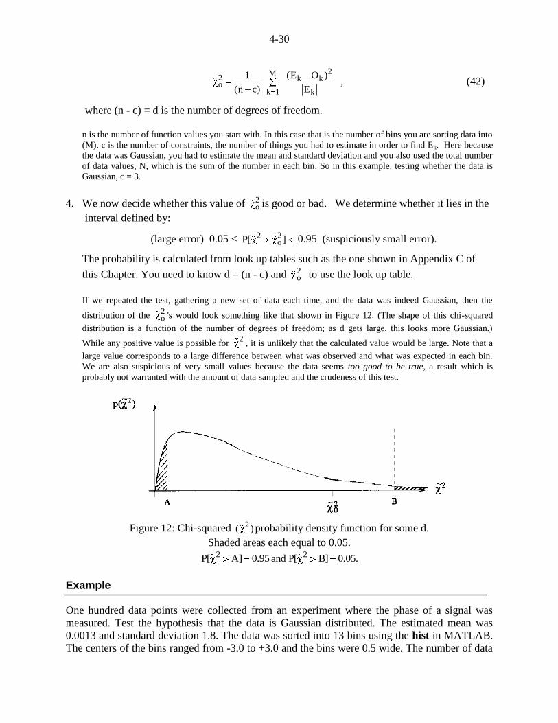
4. We now decide whether this value of 2o is good or bad. We determine whether it lies in the

interval defined by:

(large error) 0.05 < 2 2oP[ ] 0.95 (suspiciously small error).

The probability is calculated from look up tables such as the one shown in Appendix C of

this Chapter. You need to know d = (n - c) and 2o to use the look up table.

If we repeated the test, gathering a new set of data each time, and the data was indeed Gaussian, then the

distribution of the 2o 's would look something like that shown in Figure 12. (The shape of this chi-squared

distribution is a function of the number of degrees of freedom; as d gets large, this looks more Gaussian.)

While any positive value is possible for 2

, it is unlikely that the calculated value would be large. Note that a

large value corresponds to a large difference between what was observed and what was expected in each bin.

We are also suspicious of very small values because the data seems too good to be true, a result which is

probably not warranted with the amount of data sampled and the crudeness of this test.

Figure 12: Chi-squared 2( ) probability density function for some d.

Shaded areas each equal to 0.05. 2 2P[ A] 0.95 and P[ B] 0.05.

Example

One hundred data points were collected from an experiment where the phase of a signal was

measured. Test the hypothesis that the data is Gaussian distributed. The estimated mean was

0.0013 and standard deviation 1.8. The data was sorted into 13 bins using the hist in MATLAB.

The centers of the bins ranged from -3.0 to +3.0 and the bins were 0.5 wide. The number of data

4-31

points in each bin, starting from the bin centered on -3.0, was: 7, 4, 12, 8, 4, 7, 14, 10, 9, 7, 6, 12,

8.

Solution Use a mean = 0.0, standard deviation of data = 1.8, standard deviation of estimated mean = 0.18,

and so the third and fourth decimal places in the estimated mean are not significant. For the chi-

squared analysis the first and last bins were expanded to - and + , respectively.

Shown in Figure 13 is the estimated probability density function derived from dividing the

number of values in each bin by (bin width total number of data points) = 0.5 ( 100 = 50. Also

shown is a Gaussian probability density function having a mean of 0.0 and a standard deviation

of 1.8.

Figure 13: Estimated and Gaussian probability density functions.

The expected values were calculated from equation (40), utilizing the erf program in MATLAB.

You could also do these calculations using the table in Appendix A. The data is shown in the

Table below.

Bin Limits Calculated and Measured Data

i 1x ix kO kE Error

-∞ -2.75 7 6.9657 0.0002

-2.75 -2.25 4 4.3567 0.0292

-2.25 -1.75 12 6.0188 5.9439

-1.75 -1.25 8 7.7387 0.0088

-1.25 -0.75 4 9.2607 2.9884

-0.75 -0.25 7 10.3139 1.0648

-0.25 0.25 14 10.6910 1.0242

0.25 0.75 6 10.3139 1.8044

0.75 1.25 4 9.2607 2.9884

1.25 1.75 8 7.7387 0.0088

1.75 2.25 6 6.0188 0.0001

2.25 2.75 12 4.3567 13.4093

2.75 + 8 6.9657 0.1536

4-32

Check that the calculations are correct by summing the Ek’s, the result should equal the number

of data points (100).

d = M – 3 = 13 – 3 = 10. 2o = 2.9424

From Appendix C,

2oP [ 2.9424] 0.002 , expressed as 0.2% in the table.

Therefore we reject the hypothesis that the data was Gaussian distributed at the 5% significance

level.

For your interest, listed below is the MATLAB m-file used to do the calculations and plotting for

this example.

% ch4exchi.m program to do a chi squared example

% % Data generation for example. n=100

rand('seed',sum(100000*clock)) x=pi*2*(rand(1,n)-0.5); %

% Definition of bins, based on Eq. (40), Chapter 4 xbin=(-3.:0.5:3.); wid=0.5;

wid2=0.25 % % Calculation of histogram, y contains no. of points in each bin.

% nen contains the bin centers. M is the number of bins [y,nen] = hist(x,xbin); [a,M]=size(nen)

% % Data statistics. sigx=std(x);

me=mean(x); % % Calculation of the area of each bin

for i=1:M; % % First normalize bin boundaries for erf function.

xt=max([abs(nen(i)-wid2),abs(nen(i)+wid2)])/(sqrt(2)*sigx); xb=min([abs(nen(i)-wid2),abs(nen(i)+wid2)])/(sqrt(2)*sigx); %

% If this is the first or last bin calculate the additional % area.

if i==1

xxl=n*0.5*(1-erf(xt)); elseif i==M xxu=n*0.5*(1-erf(xt));

end % % Now calculate the areas associated with each boundary,

% subtract unless the mean is contained in the bin, % then add. if ( me>=(nen(i)-wid2) & me<=(nen(i)+wid2) )

e(i)=n*0.5*(erf(xt)+erf(xb));

4-33

else

e(i)=n*0.5*(erf(xt)-erf(xb));

end % end

% % Now correct first and last bin to add the tails. e(1)=e(1)+xxl;

e(M)=e(M)+xxu; % % Check that e sums to n, the number of data points.

[n sum(e)] % % Calculate the bin boundaries.

binl=nen-wid2; binu=nen+wid2; %

% Calculate the error and the chi-squared statistic. erro=(y-e).^2./abs(e);

chi=sum(erro)/(M-3)

% % Now tabulate the results in a diary file. !rm diary

diary on [binl' binu' y' e' erro'] diary off

% % Plot the estimated and the Gaussian distributions. % Put the measured data into a bar chart form.

[xx,yy]=bar(nen,y); % % Normalize yy (histogram of y) to form p hat (x).

yy=yy/(n*wid); % % Calculate the Gaussian from the estimated mean and standard deviation.

xgr=(-500:500)/100;

ygr=(1./(sqrt(2*pi)*sigx))*exp((-(xgr-me).^2)/(2*sigx^2)); %

% Plot the histogram and the Gaussian with text annotation. plot(xx,yy,xgr,ygr) xlabel('x - measured values')

ylabel('p(x)') gtext('Measured pdf') gtext('Gaussian pdf')\fR

SUMMARY

In this Chapter we have given you a brief introduction to statistics. Many Measurements texts

cover this material as well as Statistics and Error Analysis texts. In putting these notes together

the references listed below were used.

Here we have considered ways of describing a quantity that is random, basically through its

probability density function. Often we don't know this, but we can estimate the mean and

4-34

standard deviation of the data, which is a measure of what value the data is centered on and how

much variation is present. Often it is assumed that the data has a Gaussian distribution; we have

looked at the chi-squared test of this assumption. We developed confidence intervals for the true

value of the quantity that we are trying to measure based on the estimated mean and standard

deviation of the data.

We then considered what happens when we have a function of one or several quantities that

are random variables, and how the variation propagates through the function to produce

variability in the output of the function. In static calibration, where we compare the amplitude of

the output of a measurement system with the amplitude of the input, we often approximate the

input-output relationship with a straight line. In Chapter 2 we did this is a very qualitative

manner, in this chapter we derived the formulae for calculating the intercept and gradient of the

best fit straight line, given a set of (Xi, Yi) calibration measurements. Also we derived formulae

for the variation in these intercept (bias) and gradient (sensitivity) estimates, as well as

describing a measure (R2), which is an indicator of how well the model fits the data.

References

1. J. R. Taylor, An introduction to error analysis, University Science Books, Oxford

University Press, 1982.

2. T. G. Beckwith, G. Thomas, Mechanical measurements, Addison-Wesley, 1993.

3. R. S. Figliola and D. E. Beasley, Theory and design for mechanical measurements,

Wiley, 1995.

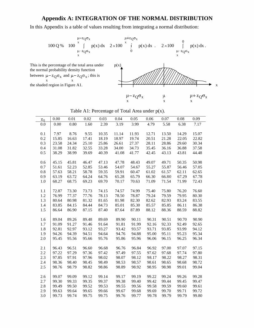
Appendix A: INTEGRATION OF THE NORMAL DISTRIBUTION

In this Appendix is a table of values resulting from integrating a normal distribution:

Q x Q xx x

Q x Q xx x

z z0

z 0 z

100 Q % 100 p(x) dx 2 100 p(x) dx . 2 100 p(x) dx .

This is the percentage of the total area under p(x)

the normal probability density function

between Q xx

z and Q xx

z ; this is

the shaded region in Figure A1. x

Q xx

z

x

Q xx

z

Table A1: Percentage of Total Area under p(x).

zQ 0.00 0.01 0.02 0.03 0.04 0.05 0.06 0.07 0.08 0.09

0.0 0.00 0.80 1.60 2.39 3.19 3.99 4.79 5.58 6.38 7.17

0.1 7.97 8.76 9.55 10.35 11.14 11.93 12.71 13.50 14.29 15.07

0.2 15.85 16.63 17.41 18.19 18.97 19.74 20.51 21.28 22.05 22.82

0.3 23.58 24.34 25.10 25.86 26.61 27.37 28.11 28.86 29.60 30.34

0.4 31.08 31.82 32.55 33.28 34.00 34.73 35.45 36.16 36.88 37.58

0.5 38.29 38.99 39.69 40.39 41.08 41.77 42.45 43.13 43.81 44.48

0.6 45.15 45.81 46.47 47.13 47.78 48.43 49.07 49.71 50.35 50.98

0.7 51.61 52.23 52.85 53.46 54.07 54.67 55.27 55.87 56.46 57.05

0.8 57.63 58.21 58.78 59.35 59.91 60.47 61.02 61.57 62.11 62.65

0.9 63.19 63.72 64.24 64.76 65.28 65.79 66.30 66.80 67.29 67.78

1.0 68.27 68.75 69.23 69.70 70.17 70.63 71.09 71.54 71.99 72.43

1.1 72.87 73.30 73.73 74.15 74.57 74.99 75.40 75.80 76.20 76.60

1.2 76.99 77.37 77.76 78.13 78.50 78.87 79.24 79.59 79.95 80.30

1.3 80.64 80.98 81.32 81.65 81.98 82.30 82.62 82.93 83.24 83.55

1.4 83.85 84.15 84.44 84.73 85.01 85.30 85.57 85.85 86.11 86.38

1.5 86.64 86.90 87.15 87.40 87.64 87.89 88.12 88.36 88.59 88.82

1.6 89.04 89.26 89.48 89.69 89.90 90.11 90.31 90.51 90.70 90.90

1.7 91.09 91.27 91.46 91.64 91.81 91.99 92.16 92.33 92.49 92.65

1.8 92.81 92.97 93.12 93.27 93.42 93.57 93.71 93.85 93.99 94.12

1.9 94.26 94.39 94.51 94.64 94.76 94.88 95.00 95.11 95.23 95.34

2.0 95.45 95.56 95.66 95.76 95.86 95.96 96.06 96.15 96.25 96.34

2.1 96.43 96.51 96.60 96.68 96.76 96.84 96.92 97.00 97.07 97.15

2.2 97.22 97.29 97.36 97.42 97.49 97.55 97.62 97.68 97.74 97.80

2.3 97.85 97.91 97.96 98.02 98.07 98.12 98.17 98.22 98.27 98.31

2.4 98.36 98.40 98.45 98.49 98.53 98.57 98.61 98.65 98.68 98.72

2.5 98.76 98.79 98.82 98.86 98.89 98.92 98.95 98.98 99.01 99.04

2.6 99.07 99.09 99.12 99.14 99.17 99.19 99.22 99.24 99.26 99.28

2.7 99.30 99.33 99.35 99.37 99.38 99.40 99.42 99.44 99.45 99.47

2.8 99.49 99.50 99.52 99.53 99.55 99.56 99.58 99.59 99.60 99.61

2.9 99.63 99.64 99.65 99.66 99.67 99.68 99.69 99.70 99.71 99.72

3.0 99.73 99.74 99.75 99.75 99.76 99.77 99.78 99.79 99.79 99.80

4-36

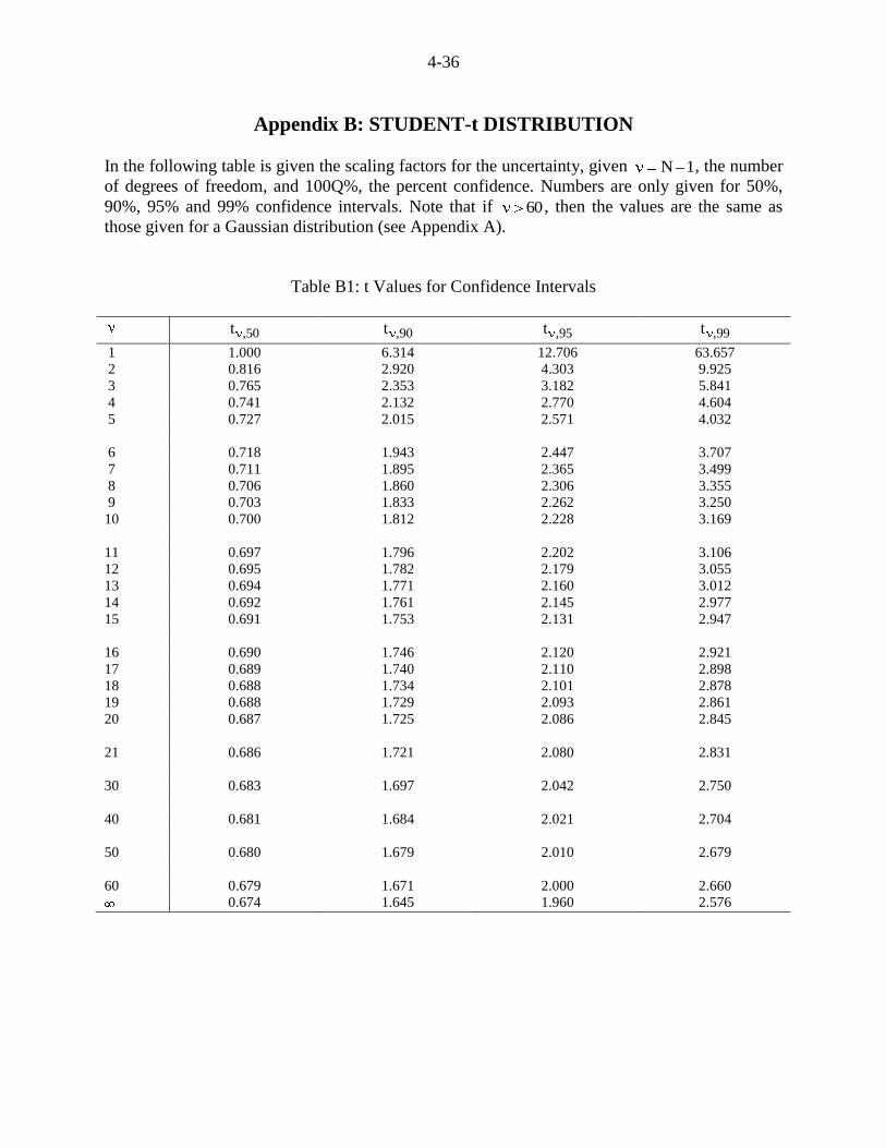
Appendix B: STUDENT-t DISTRIBUTION

In the following table is given the scaling factors for the uncertainty, given N 1, the number

of degrees of freedom, and 100Q%, the percent confidence. Numbers are only given for 50%,

90%, 95% and 99% confidence intervals. Note that if 60 , then the values are the same as

those given for a Gaussian distribution (see Appendix A).

Table B1: t Values for Confidence Intervals

,50t ,90t ,95t ,99t

1 1.000 6.314 12.706 63.657

2 0.816 2.920 4.303 9.925

3 0.765 2.353 3.182 5.841

4 0.741 2.132 2.770 4.604

5 0.727 2.015 2.571 4.032

6 0.718 1.943 2.447 3.707

7 0.711 1.895 2.365 3.499

8 0.706 1.860 2.306 3.355

9 0.703 1.833 2.262 3.250

10 0.700 1.812 2.228 3.169

11 0.697 1.796 2.202 3.106

12 0.695 1.782 2.179 3.055

13 0.694 1.771 2.160 3.012

14 0.692 1.761 2.145 2.977

15 0.691 1.753 2.131 2.947

16 0.690 1.746 2.120 2.921

17 0.689 1.740 2.110 2.898

18 0.688 1.734 2.101 2.878

19 0.688 1.729 2.093 2.861

20 0.687 1.725 2.086 2.845

21 0.686 1.721 2.080 2.831

30 0.683 1.697 2.042 2.750

40 0.681 1.684 2.021 2.704

50 0.680 1.679 2.010 2.679

60 0.679 1.671 2.000 2.660

0.674 1.645 1.960 2.576

4-37

Appendix C: INTEGRATION OF THE 2 DISTRIBUTION

Tabulated below is 2 2o100 P[ ] .

d = n – c is the number of degrees of freedom. n is the number of function values, equal to the

number of bins if you are testing to see if the data is Gaussian. c is the number of constraints

which usually equals 3, when the hypothesis is that the data is Gaussian distributed. 2o is the

chi-squared statistic that you calculated from your test.

Recall that you are probably interested in obtaining a value between 5 (errors very large) and 95

(errors suspiciously small) for an acceptance of your hypothesis.

2o

d 0.0 0.5 1.0 1.5 2.0 2.5 3.0 3.5 4.0 4.5 5.0 5.5 6.0 8.0 10.0

1 100 48 32 22 16 11 8.3 6.1 4.6 3.4 2.5 1.9 1.4 0.5 0.2

2 100 61 37 22 14 8.2 5.0 3.0 1.8 1.1 0.7 0.4 0.2 - -

3 100 68 39 21 11 5.8 2.9 1.5 0.7 0.4 0.2 0.1 - - -

4 100 74 41 20 9.2 4.0 1.7 0.7 0.3 0.1 0.1 - - - -

5 100 78 42 19 7.5 2.9 1.0 0.4 0.1 - - - - - -

0.0 0.2 0.4 0.6 0.8 1.0 1.2 1.4 1.6 1.8 2.0 2.2 2.4 2.6 2.8 3.0

1 100 65 53 44 37 32 27 24 21 18 16 14 12 11 9.4 8.3

2 100 82 67 55 45 37 30 25 20 17 14 11 9.1 7.4 6.1 5.0

3 100 90 75 61 49 39 31 24 19 14 11 8.6 6.6 5.0 3.8 2.9

4 100 94 81 66 52 41 31 23 17 13 9.2 6.6 4.8 3.4 2.4 1.7

5 100 96 85 70 55 42 31 22 16 11 7.5 5.1 3.5 2.3 1.6 1.0

6 100 98 88 73 57 42 30 21 14 9.5 6.2 4.0 2.5 1.6 1.0 0.6

7 100 99 90 76 59 43 30 20 13 8.2 5.1 3.1 1.9 1.1 0.7 0.4

8 100 99 92 78 60 43 29 19 12 7.2 4.2 2.4 1.4 0.8 0.4 0.2

9 100 99 94 80 62 44 29 18 11 6.3 3.5 1.9 1.0 0.5 0.3 0.1

10 100 100 95 82 63 44 29 17 10 5.5 2.9 1.5 0.8 0.4 0.2 0.1

11 100 100 96 83 64 44 28 16 9.1 4.8 2.4 1.2 0.6 0.3 0.1 0.1

12 100 100 96 84 65 45 28 16 8.4 4.2 2.0 0.9 0.4 0.2 0.1 -

13 100 100 97 86 66 45 27 15 7.7 3.7 1.7 0.7 0.3 0.1 0.1 -

14 100 100 98 87 67 45 27 14 7.1 3.3 1.4 0.6 0.2 0.1 - -

15 100 100 98 88 68 45 26 14 6.5 2.9 1.2 0.5 0.2 0.1 - -

16 100 100 98 89 69 45 26 13 6.0 2.5 1.0 0.4 0.1 - - -

17 100 100 99 90 70 45 25 12 5.5 2.2 0.8 0.3 0.1 - - -

18 100 100 99 90 70 46 25 12 5.1 2.0 0.7 0.2 0.1 - -

19 100 100 99 91 71 46 25 11 4.7 1.7 0.6 0.2 0.1 - - -

20 100 100 99 92 72 46 24 11 4.3 1.5 0.5 0.1 - - - -

22 100 100 99 93 73 46 23 10 3.7 1.2 0.4 0.1 - - - -

24 100 100 100 94 74 46 23 9.2 3.2 0.9 0.3 0.1 - - - -

26 100 100 100 95 75 46 22 8.5 2.7 0.7 0.2 - - - -

28 100 100 100 95 76 46 21 7.8 2.3 0.6 0.1 - - - -

30 100 100 100 96 77 47 21 7.2 2.0 0.5 0.1 - - - -

4-38