Chapter 4

Schrodinger Picture Formalism

4.1 Introduction

Variational methods in functional Schr6dinger picture have been shown to

be very useful in the study of detailed structures of the quantum fields,

both for the bosonic and fermionic field theories [39,42 ,47]. Recently vari-

ous interesting applications of this formalism has been presented . In (2+1)

dimensional Thirring model [52]. Gaussian approximation provides better

information than the large -N approximation. it has been used to derive

(2+1) dimensional effective potential in Liouville model 1461. Quantum field

theoretic analysis of inflation dynamics in a (2+1) dimensional universe has

been worked out using this method 1711. Taking into consideration the re-

cent interest of the formalism in (2+1) dimensional theories we propose to

apply the method to the most general renotmalisable scalar theory in (2+1)

53

54 CHAPTER 4. SCHR6DINGER PICTURE FORMALISM

dimensions that is a V model.We find that the effective potential expression

that emerges using functional SchrBdinger picture is same as that derived

using CJT formalism in chapter 2.

4.2 Effective Action

We propose to apply the formalism to a +e model and since 918 coupling

effects show up only at the three loop level we write the expression up to

three loops [chapter 1,egn. 1.41].

Jdt [jn I - 2 + f .y EG-

2J EGE-J t)

-2V G(z, U,t)" + ill(3)G(z,z,t), -

G(x, z, t)Z -1B (^) J Gs(z, . t)

In this chapter we follow the standard practice in the functional Schrgdinger

picture representing expectation values as 6 equivalent to shift 0 used in

preceding chapters. Identifying the first term as the classical action and per-

4.3. STATIC EFFECTIVE POTENTIAL

forming variations we obtain

bT = 0 --+ rt(.T, t) = vsO(--, t) - W) (0)

55

-2113)(^)G(x,x,t) - V-5)(^)G2(x , x,t) (4.2)

=0 E(z t +2S

ExztEx t

= G-2 (z, y, t) + {v_2 4 )(^)G(x, x, t)

-4JAG) (^)G2(x, x, t)] F(x - y)

Y, t}_ 0 --^ G(x, y, t) = 2 {J G(z, z,t)>.(x, v,t)SE (

+o,(x, z, t)G(z, y, t)J

4.3 Static Effective Potential

It has been shown that renormalization of time-dependent equations can be

achieved along the same lines of the renormalization of the static effective

potential, We therefore evaluate the static effective potential for 4 model

at zero temperature. This can be achieved by taking 4 to be `x' independent

56 CHAPTER 4. SCHRBDINGER PICTURE FORMALISM

and putting E = 0. The classical potential for the model is given in chapter

2 (egn.2.1]. The effective potential is given by given in chapter 2. By evalu-

ating the derivatives we get

vs!!( , G) _ m2^2+ (i4 + & ¢j8

+2m2

+4

.P + c 4 G(x, x)48

+ g^2) G2 (z, X) + Gg(x, x)+ g_ 48

+8I trG-1(x, x) - VsG(x, x) (4.5)

By performing variation with respect to G the gap equation is obtained.

G-2(x, v) - -b2 + m2 +2

fi2 + ^4

24

+ 2 G(x, y) + 4^1G'(x,y)+ _48 G (x, v) 6(x - y)

Assuming translation invariance the Fourier transform of a function is de-

fined as

4.3. STATIC EFFECTIVE POTENTIAL 57

f&kef(k) (4.7)^) = J 2

G(x, X)J 2 2 [0 + m2 + 2 2+ 24 4 x

G(z, z) + 4 G(z, z) + -g4G2(r, x) - (4.8)

fk;;

2(k2 + M2) (4.9)

where an anzatz is fixed for G in terms of an effective mass [chapter 2,egn.2.81.

The effective mess M is treated here as a variational parameter which is

dependent-The static effective potential can be written as

V.!!(^, = j (k2+M2)+

1 mB + + Ls ^°2 41 e1

+2mB 2 _ L0' G(z, X) +

+ g + Q^z G (s,z) + 4-C &(z,x) (4.10)

58 CHAPTER 4. SCHRODINGER PICTURE FORMALISM

Eqn (4. 10) shows that the effective potential expression obtained here is

the same as the one obtained using Gaussian effective potential approach

[17]. This is only natural since when time dependence is not taken into

account definitions of effective action in both the approaches coincide. From

the earlier analysis [chapter 21 it also becomes clear that the formalism is

equivalent to CJT approach at zero temperature . Both the equations differ

by a tc term. This term does not contribute when daisy and super daisy

diagrams are considered through Hartee-fock approximation. At ¢4 level

both the approaches are exactly identical.

Considering the first and second terms alone of egn(4.10) it can be seen

that one loop effective potential result is contained in the expression with

the mass term replaced by the effective mass . Identity with the Gaussian

effective potential results become more transparent if we make the following

correspondence in notation.

G(x,^) -► 10 = -F 1 (4.11)77"2(P+m2)

2 ](k2 + m2) -' Il (4.12)

M ---; ci (4.13)

4.4. FINITE TEMPERATURE CALCULATION FOR 4 6 MODEL 59

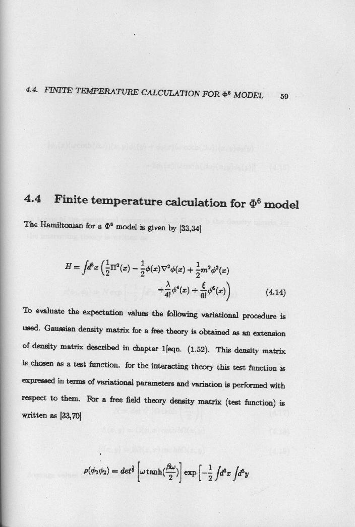
4.4 Finite temperature calculation for V model

The Hamiltonian for a 46 model is given by [33,341

H= fiax (rr2(a) -1 O(r)V20(x) + 1 202(x}

+4 04(X) + 61^b6(x) (4.14)

To evaluate the expectation values the following variational procedure is

used . Gaussian density matrix for a free theory is obtained as an extension

of density matrix described in chapter 1[egn . (1.52). This density matrix

is chosen as a test function . for the interacting theory this test function is

expressed in terms of variational parameters and variation is performed with

respect to them. bbr a free field theory density matrix (test function) is

written as 133,701

P(0102) = deti [wtan1i ( )] exp I-2 Jdz fdsy

60 CHAPTER 4. SCHRODINGER PICTURE FORMALISM

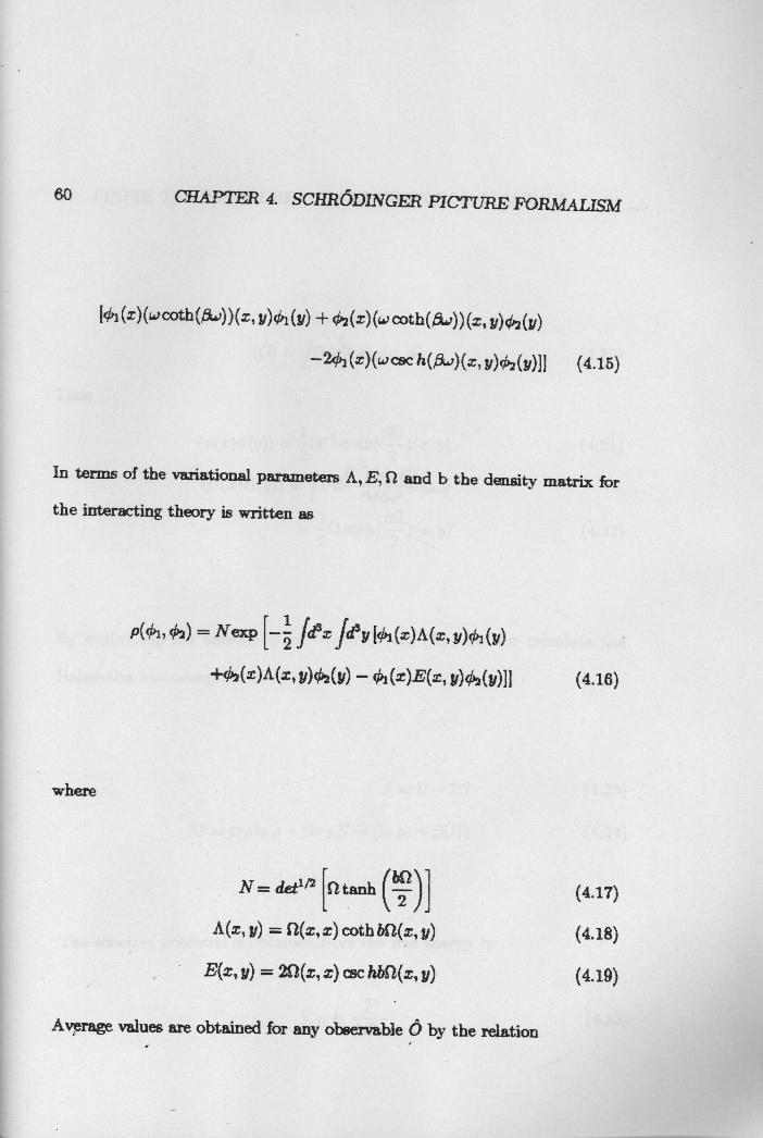
^ (z}(wcoth (f '})(z, y) (y) + 02(z)(wcoth ( OW)) (z, y)d2(y)

-201(x) (wcsc h(&)(x, y)02(y))) (4.15)

In terms of the variational parameters A, E, Il and b the density matrix for

the interacting theory is written as

P(01, 02) = NeXp L 2 Id3x jd5y 10, (x)A(x y)41 (3►)

+(x)A(x, y)02(y) - 01(x)E(x, y)4(?/)])

where

(4.16)

N= det1/2 [cuanh ( 2KI)l

(4.17)

A (x, y) = II(x, z) coth bf2(x, y) (4.18)

E(x, y) = 20(z, x) csc hbfl(x, y) (4.19)

Average values are obtained for any observable 6 by the relation

4.4. FINITE TEMPERATURE CALCULATION FOR 4 MODEL 61

(O) = JV(*b)p (ci, 0) (4.20)

Thus

(II(x)II(y))

bfI= 2S2coth ( )(x,y)

(4.21)

(4.22)

By evaluating the entropy S = - (p In p) and (B ), we can calculate the

Helmholtz free energy F:

F= U- IS (4.23)

OF = trp in p + 'pH = (In ) + 3(H)

The effective potential is obtained from the free energy by

V.ff = fda^F

(4.24)

(4.25)

62 CHAPTER 4. SCHRODINGER PICTURE FORMALISM

The evaluation of the entropy function and the expectation value of the

Hamiltonian for a 0' theory has already been given 1331.Additional terms

appearing in the expectation value of 06 theory are a 4 dependent part and

a 0 independent part. We consider only the 02 independent part because in

the CJT formalism we used the Hartee Fock approoamation which eliminates

the 99 dependent term.

A [dYx (m2c2= +6^^e

+ fcr 4 ci + (_,72 + m2 + 02 Q-1 coth (X, X)

+32(rn1 coth (x, z) 0-1 coth MTZ (z, z) +

+-L (in ' Goth b2l

) (z, z) 0-1 cothho

)(z, z)

SZ-' coth ) (x, x) (4.26)

Taking the already computed value of entropy the expression for free energy

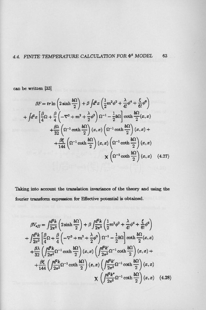
4.4. FINITE TEMPERATURE CALCULATION FOR 4 MODEL 63

can be written 1331

.OF = tr In 2 Binh b2 + 0 i fz 2m2 402 + 4! ^' + 6! 0)l

1+ ^[ ii+(_V2+m2+) 12-1 - 2MtJ coth b"2 (x, X)

+

32

(cz-I coth!S2

(x , x) 0-1 coth ^) (x, x) +2)

+ fl- 1 Goth (x , x) (n_1 coth ) bo) (x , X)144 2 2

cothb)

(x, x) (4.27)

Taking into account the translation invariance of the theory and using the

fourier transform expression for Effective potential is obtained.

st;f=,2 (2sinii)+PJ!^) 2 l(m2+4+c)

27r2 2 2A 2 4

J 2 4 SZ + 4 (_v2+m2+2) S2-' - 2bf oath (x, 2)

+ 32(J cr1 coth (x, x) c-1 coth ! (2, 2) +

+144 J 2-I coth'o (s, x) (j ,̂ cr' coth (x, x)

X J ft-I Goth (x, x) (4.28)

64 CHAPTER 4. SCHRODINGER PICTURE FORMALISM

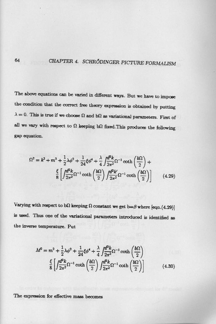
The above equations can be varied in different ways . But we have to impose

the condition that the correct free theory expression is obtained by putting

A = 0. This is true if we choose fl and bR as variational parameters . First of

all we vary with respect to fl keeping bit fixed.This produces the following

gap equation.

Q2 = + m2 +

2

+ 24t` 4 + 4 J 2^rk Q coth +^2^

[j . _icoth 1 2 i-1 coth (4.29)

} 2 lJ

Varying with respect to bSt keeping n constant we get b`0 where [egn.(4.29)]

is used . Thus one of the variational parameters introduced is identified as

the inverse temperature. Put

M _m2+2acb2+24 V +4J2 Q-1 c0 !22

-1

8 242 Goth (In)

j r' coth2 2 (4.30)

The expression for effective mass becomes

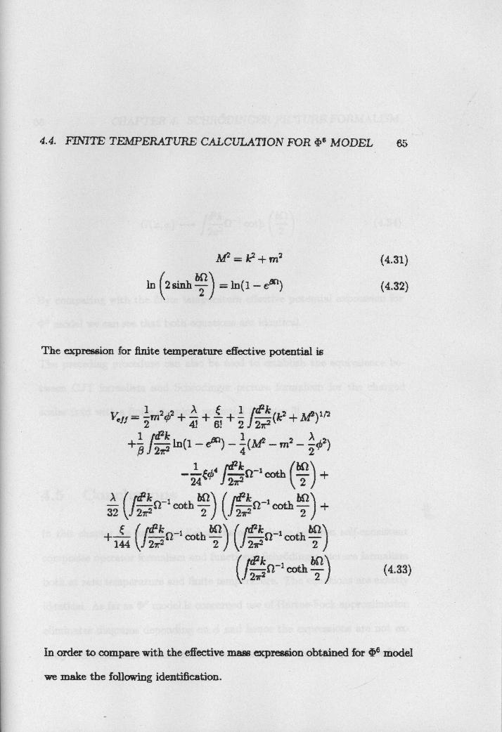
4.4. FINITE TEMPERATURE CALCULATION FOR 4 MODEL

M2 =k2+m2

In 2 Binh 2 ` =1n(1- em)

The expression for finite temperature effective potential is

2 2 A 1 Id2k 1Yell= 2m +41 +6!+2J (k2+AP) R

+ f 2 ln(1 - ems) - (M2 - m2 - 2 ¢2)

J 7 7_4 1 k D-' coth (m) -+

.

2 (rk

r2 -1 coth 2 (J4tr' c^oth 2 +

144 f^11-1 Goth

) (fl i Goth )

ftPkQ-' coth

MI)

65

(4.31)

(4.32)

(4.33)

In order to compare with the effective mass expression obtained for 4e model

we make the following identification.

66 CHAPTER 4. SCHRBDINGER PICTURE FORMALISM

J 2:-i cosh ( ) (4.34)

By comparing with the finite temperature effective potential expression for

46 model we can see that both equations are identical.

The preceding procedure can also be used to establish the equivalence be-

tween CJT formalism and Schrodinger picture formalism for the charged

scalar field with a finite chemical potential [chapter 31

4.5 Conclusions

In this chapter we have established the equivalence between self-consistent

composite operator formalism and functional Schrodinger picture formalism

both at zero temperature and finite temperature. The equations are exactly

identical. As far as 4 model is concerned use of Hartee-Flock approximation

eliminates diagrams depending on cb and hence the expressions are not ex-

actly identical . This raises certain doubts about the validity of Hartee-Fock

4.5. CONCLUSIONS 67

approximation in (V model. But when the purpose is to include daisy and

superdaisy diagrams in the summation and when we consider only scalar

models the approximation is valid.