5-1

C h a p t e r 5

ASPERITY MODEL FOR INTERSEISMIC DEFORMATION IN

NORTHEASTERN JAPAN

5.1 Introduction

In the last century, several large (M > 7) earthquakes have occurred on the megathrust

interface along the Japan Trench, offshore of Japan's Tohoku region. Published

earthquake source inversions based on seismological and high-rate GPS data suggest that

the earthquakes off Miyagi [Miura et al., 2006; Umino et al., 2006], Sanriku [Tanioka et

al., 1996; Nakayama and Takeo, 1997], and Tokachi [Robinson and Cheung, 2003;

Hamada and Suzuki, 2004; Miyazaki et al., 2004; Satake et al., 2006] occurred repeatedly

over roughly the same region of the subduction megathrust. In contrast, inversions of

geodetic data from interseismic periods produce models that are locked over more

spatially extensive regions [e.g., Bürgmann et al., 2005; Suwa et al., 2006; Chlieh et al.,

2008b]. These broad and smooth regions are in contrast to the smaller discrete asperities

indicated by earthquake source studies, and may be a consequence of lack of model

resolution and a resulting need for regularization that is inherent to the use of onshore

geodetic data. Alternatively, the differences may imply the potential for a large

earthquake in the future. Thus, the different levels of apparent coupling implied by these

two classes of models have very different implications for regional seismic hazard

(Figure 1-1). Here, we explore whether post-seismic slip resulting from mechanical

coupling of the inferred seismic asperities alone can reconcile this apparent difference in

seismic hazard estimates. We do not seek to model the complex dynamics of rupture

nucleation, interaction between asperities, or rupture propagation [see for e.g., Rice,

1993; Lapusta and Rice, 2003; Hori, 2006; Kato, 2008; Perfettini and Ampuero, 2008].

5-2

Several studies have recently attempted to constrain post-seismic creep on faults from

inversions of high-rate geodetic data. These studies either tested the inferred postseismic

creep for consistency with specific fault rheologies [e.g., Miyazaki et al., 2004; Hsu et al.,

2006], or by modeling this inferred creep as a response of the fault to coseismic tractions,

inferred its rheological properties [e.g., Johnson et al., 2005; Perfettini and Avouac,

2007]. However, the latter modeling studies were restricted to planar faults with rate-

state frictional rheologies, and used ad hoc, but physically based initial conditions — for

example, both studies assume that the entire fault slips at the plate convergence rate just

before an earthquake. Below, we show that this assumption is not true, especially within

the “stress-shadow” regions surrounding the asperities. While Perfettini and Avouac

[2007] assumed that fault behavior was partitioned between an upper seismogenic zone

and a lower brittle creep zone, Johnson et al. [2005] allowed coseismic and post-seismic

slip to occur along the entire modeled fault surface.

Using a Boundary Element Method (BEM) model, Bürgmann et al., [2005] tested the

effect of stress-shadows from “pinned” asperities on horizontal velocity predictions for

the subduction zone off Kamchatka for several asperity models. They assumed that all

areas outside the asperities slip freely (i.e., with zero driving shear stress, which is

unphysical), resulting in a stress-shadow that is primarily located up-dip from each

asperity. Since they ignore fault friction, they cannot model slip evolution around the

asperities over the seismic cycle — especially down-dip of, and laterally (along strike)

from, the asperity. Recently, Hetland et al. [2010] and Hetland and Simons [2010]

developed an internally consistent 3D mechanical model of stress-dependent interseismic

creep along the megathrust, considering both frictional and viscous fault rheologies. The

stresses in this model evolve as a consequence of long-term deformation of the system

(“spin-up”), and are determined by cumulative slip on the fault over this evolutionary

period. Further, their model allows localized regions (“asperities”) of the fault surface to

only slip coseismically at pre-assigned rupture times, thus allowing them to model the

known spatio-temporal distribution of large earthquakes (similar to Bürgmann et al.,

[2005]). Unlike Bürgmann et al., [2005], however, slip in the regions surrounding these

asperities is controlled by the specific fault rheology being assumed. They used “toy”

5-3

models to show that asperities are surrounded by a “halo” of very low creep-rates (a

“stress-shadow” effect) late in the seismic cycle, which can potentially result in a

relatively smooth and long wavelength surface velocity field.

As described in detail in the previous chapter, we extend this approach to an arbitrary3D

fault surface experiencing an arbitrary sequence of ruptures. We apply this extended

model to northern Japan, to investigate whether this “physical” smoothing preserves any

signature of the original asperities, in comparison to the artificial smoothing produced by

model regularization in inversions of interseismic geodetic data. Here, we test the

hypothesis that on inferred asperities along the Japan Trench megathrust, mechanical

coupling alone is sufficient to explain available geodetic observations or alternatively,

that these data require additional regions on the megathrust to be coupled. Underlying

our analysis is the assumption that known asperities persist across multiple earthquake

cycles.

In the following sections, we briefly review the forward modeling approach (see Hetland

et al. [2010] for details), discuss the criteria used to determine the extent and rupture

interval of each asperity chosen, present model “spin-up” and “convergence”, and finally,

present results of our hypothesis test. The results presented here are meant to

demonstrate the applicability of our approach for simulating realistic 3D fault surfaces.

More thorough parameter-space searches are planned to be carried out in the near future

to refine the analysis presented here.

5.2 Summary of the forward modeling approach

As discussed in Chapter 4, Hetland et al. [2010] cast the relationship between slip-rate

and fault tractions for various rheologies in the following dimensionless form:

)','(' ατfs = (1)

where, α΄ is a strength parameter that depends on the rheology. For linear viscous

rheology,

5-4

'

')','('

ατατ == fs . (2)

Thus, late in the cycle, when most of the fault is slipping at the loading rate, the mean

dimensionless shear tractions along the fault surface will equal the dimensionless strength

parameter, α΄. In Chapter 4, we estimated a typical range of values for α' as 0.1 to 10.

For rate-dependent rheology,

( )

′′

= −

ατρ sinh' es (3)

where, ρ = f0/(a-b), and α = (a-b)σ0*. For the results presented below, we assume a

uniform σ0*. Hetland and Simons [2010] demonstrated that the effect of including

variable normal tractions (that is, normal tractions due to the evolving slip distribution

over the fault surface) was negligible, unless the static strength of the fault is assumed to

be large (cf. Figure 3 of Hetland and Simons [2010]). Even in the case where the fault is

statically strong, the effect of variable tractions is significant only updip of the asperity,

far from typical geodetic observations. However, they consider an effective (or

reference) stress, σ0*, that is much higher than the imposed coseismic traction

perturbation. If σ0* is small, as is thought to be typical of most subduction zones (owing

to pore-pressure effects [e.g., Kanamori, 1971; Hyndman and Wang, 1993]), then

variable normal tractions will significantly influence slip-evolution over the fault surface.

But their effect will be pronounced in the vicinity of the asperities and especially during

the period immediately following a rupture.

From Equation 3 we can deduce that late in the cycle, when most of the fault is slipping

at the loading rate, the mean dimensionless shear tractions along the fault surface will

equal the product of ρ and the dimensionless strength parameter, α' — that is,

τss' = ρ α' (4)

Plate loading and frictional stresses are then in equilibrium over most of the “active” fault

surface (over which slip evolves), except around the regularly rupturing asperities. This

5-5

product is nothing but f0σ0*/τ0, where the denominator is the characteristic rupture stress,

μS0/D0, the mean frictional resistance over the fault surface (see Chapter 4). So, α'

determines the relative static strength of the fault surface relative to the induced

coseismic stresses. In Chapter 4, we estimated a typical range of values for ρ ≈10–100,

and α ≈ 105–106 Pa. Assuming the same values as before for the non-dimensionalization

of stresses, and μ ≈ 1010 Pa, α' ≈ 0.01–0.1. At the lower end, we have a fault that is

“weak” (f0σ0* « τ0) compared to the imposed coseismic tractions, and the model spins up

quickly. On the other hand, a fault that is “strong” in comparison to the imposed

coseismic tractions results in slow spin-up of fault tractions. For α' ≈ 1, and the fault

strength is comparable to the imposed coseismic stress pulses. For realistic values of the

“damping-parameter”, ρ, noted above, the effect of the first factor on the right hand side

of equation (3) has only a minor influence on the evolution of post-seismic slip compared

to that of the second factor. However, tractions late in the seismic cycle (i.e., when the

mean fault slip-rate is close to the imposed plate velocity) are strongly dependent on both

ρ and α' (Equation 4, also see Figure 14 of Hetland et al. [2010]). Thus, changing these

two parameters allows us to explore the effect of background stresses on slip-evolution

over a spun-up seismic cycle.

In order to solve for slip evolution on the fault surface, the tractions, τ΄, everywhere on

the fault surface at any given time have to be related to coseismic slip, the far-field plate

loading rate, and any ongoing post-seismic slip along the fault itself. This is

accomplished by a discretized traction evolution equation, that can be represented in

indicial notation as,

+−=a

jijajijji KSKVts ''')'''('τ (5)

where, K΄ji are the traction kernels (i.e., tractions at patch i due to slip on patch j), and

traction (τ΄), and slip (s΄) vary both in space and in time. Also, as discussed extensively

in Chapter 2, in order to be kinematically consistent, we use a backslip rate distribution

that is everywhere tangential to the 3D fault surface (i.e., backslip with spatially varying

rake; Figure 4-6). The first term in Equation 5 accounts for ongoing fault slip and

continuous far-field plate loading, while the second term is the cumulative effect of

5-6

coseismic slip (S΄) on all asperities. Due to the kinematic nature of the imposed ruptures,

we cannot consistently model the effect of coseismic tractions due to the rupture of one

asperity on subsequent coseismic slip on an adjacent asperity. A relationship similar to

Equation 5 defines surface displacement evolution. Using indicial notation,

+−=a

jkjajkjjk GSGVtsu ''')'''(' (5)

where, G΄jk are the surface displacement kernels (or Green’s functions, i.e., displacements

at observation station k due to slip on patch j).

As discussed in Chapter 4, we use the triangular dislocation solutions [as compiled in

Meade, 2007] to compute K and G for a spatially discretized 3D fault in a homogeneous

Poission half-space. The traction evolution Equation 5 is solved together with the

appropriate constitutive relation (e.g., Equation 3), by marching in time using adaptive

time-stepping. The time-step at any given time in such an adaptive scheme is controlled

by the slip rate at that time, with larger slip rates resulting in smaller time-steps.

5.3 Asperity parameters for the Japan Trench megathrust

In this section, we discuss in detail the methodology used to estimate the location and

extent of each inferred characteristic asperity on the Japan Trench megathrust surface, as

well as its characteristic rupture interval. We are inherently assuming there is no

variability between individual ruptures on each asperity (that is, the rupture sequence is

both time- and slip-predictable), and therefore there is a characteristic rupture dimension,

characteristic coseismic slip, and hence, a characteristic rupture interval. In determining

these parameters, we try to honor, at a minimum, the latest significant (Mw>7.5) ruptures

inferred to have occurred on these asperities during the past century. Depending on the

characteristic rupture interval determined for each asperity, some of the previous ruptures

may not occur exactly at the same time as historical events. However, usually, they occur

within 5 years of their actual date – the effect of such small shifts in earlier ruptures was

5-7

not found to have a significant impact on surface displacement predictions, especially

because of the much stronger influence of the more recent event. We proceed from the

southernmost asperity of our modeling domain (Fukushima) to the northernmost

(Nemuro). A summary of estimated parameters is presented in Table 5-1.

5.3.1 Fukuyshima-oki — ruptures of 1938

In the megathrust interface off Fukushima, three large events - Mw7.4 (May, 1938), Mw

7.7 and Mw 7.8 (both in Nov 1938) — occurred in close succession. On the scale of

simulating an whole seismic cycle (~ 100 yrs), the moment release from these three

events can be considered “instantaneous”. So, combining the moment release from these

three events (estimated from long-period surface waves [Abe, 1977]) yields a moment,

M0, of 1.6×1021 N.m, equivalent to a moment-magnitude, Mw, of 8.1. Using only the

locally high-slip patches, Abe [1977] estimated stress-drop, Δσ, to be in the range ~ 2.8–

5.6 MPa. However, if we assume an equivalent single characteristic elliptical asperity

(assuming for purposes of mesh-quality, an aspect-ratio, f = (rmin/rmaj) = 0.8), with

Δσmean ~ 1 MPa (10 bar), then the characteristic semi-major axis dimension can be

estimated as:

( ) kmmr fM

maj 1261026.1).1( 531

0 =×≈Θ= Δσ (6)

resulting in a characteristic asperity area (= π rmaj rmin = π f rmaj2) ~ 4×104 km2. In

comparison, Abe [1977] estimated the combined total area for these three events (based

on first-motion data) to be ~ 1.5×104 km2. However, the corresponding rupture interval

turns out to be:

( ) )(! 1620

)(yrsT

Pmaj Vrf

MR ≈=Δ

μπ (7)

because we are assuming the same characteristic slip for every rupture event on this

asperity. Since there hasn’t been a Mw>7 earthquake off Fukushima since 1938, we

assume a recurrence interval of ~ 75 yrs for a characteristic earthquake similar to the

value assumed for the Tokachi-Oki region [Yamanaka and Kikuchi, 2003]. With this

assumption, the characteristic semi-major axis dimension becomes:

5-8

( ) kmmrRP TfV

Mmaj 60106 4

)(21

0 =×≈= Δμπ (8)

implying a stress drop of:

( ) MPaPamajrf

M 10100.1).1( 7

)( 30 =×≈Θ=Δσ , (9)

which is at the upper-bound of observed seismic stress-drops [Kanamori and Anderson,

1975]. To get a feel for the sensitivity of the above estimates to the exact value of the

plate velocity vector (which has been assumed to be between 8 and 9 cm/yr by different

researchers), we find that:

( )P

P

maj

maj

P

maj

RPPP

maj

VV

r

r

V

r

TfVM

VV

r

2221 2

10 ΔΔΔ∂

∂ −=−=−= μπ (10)

and,

( ) )(3)(

)(3)(31

)(31

0

σσ

σσσσ ΔΔΔΔ

ΔΔΔΔ∂∂ −=−=−=

maj

majmajmaj

r

rr

fMr

(11)

so, for a ~ 10% larger VP (9.2 cm/yr), rmaj will be 5% (or ~ 3 km) smaller, slip 10% (or ~

0.6 m) larger, and stress-drop, 15% (1.5 MPa) higher.

5.3.2 Miyagi-oki — ruptures of 1936, 1978, and 2005

Umino et al. [2006] infer that three ruptures on this asperity that occurred in the mid

1930s — in 1933, 1936, and 1937 (with a combined moment release of 2.6×1020 N.m,

equivalent to Mw7.5) overlapped with the western, central and eastern portions of the

Mw7.5 1978 rupture area, but with a moment of only a third of the latter event [Tanioka,

2003b]. The 2005 rupture also partially overlapped with the updip (southeastern) portion

of the 1978 rupture area [Miura et al., 2006]. We assume the 1978 Mw7.4-7.5 event as

the characteristic earthquake for this region (M0 = 1.7-3×1020 N.m estimated from

tsunami data [Tanioka, 2003b], and long-period surface waves [Seno et al., 1980]). The

stress drop, Δσ, based on localized high-slip patches was estimated to be 10 - 15 MPa.

As before, assuming a characteristic elliptical asperity having a mean stress drop, Δσmean

~ 1 MPa, the semi-major asperity dimension is:

5-9

( ) kmmr fM

maj 70107).1( 431

0 =×≈Θ= Δσ (12)

resulting in a recurrence interval for the characteristic earthquake

( ) )(! 920

)(yrsT

Pmaj Vrf

MR ≈=Δ

μπ (13)

Since the next major event after the 1933–37 sequence did not occur until the 1978 event,

we estimate a semi-major asperity dimension, instead, assuming a rupture interval of ~40

years (the 2005 event may be consistent with the 1933–37 sequence in that it ruptured

only one part of the characteristic asperity, and subsequent events may follow to rupture

the rest of the characteristic asperity) to be

( ) kmmrRP TfV

Mmaj 35105.3 4

)(21

0 =×≈= Δμπ (14)

implying a mean stress drop

( ) MPaPamajrf

M 9109).1( 6

)( 30 =×≈Θ=Δσ , (15)

which is, again, near the upper-bound of observed seismic stress-drops [Kanamori and

Anderson, 1975]. Another way to estimate the characteristic asperity dimension in this

case is by assuming that the mean stress-drops and asperity shapes in the 2005 and 1978

events are similar. In this case, an estimate can be made of the 1978 (characteristic)

asperity size relative to the well-determined asperity size for the 2005 Mw7.2 event (M0 =

1.7-7×1019 N.m estimated from GPS and seismic data [Miura et al., 2006]):

( ) ( )( ) kmrr

M

Mmajmaj

rf

M

rf

M

majmaj

35

).1().1(

31

)2005(0

)1978(0

32005,

)2005(0

31978,

)1978(0

2005,1978,

)()(20051978

≈=

Θ=Θ=Δ=Δ σσ (16)

which agrees almost exactly with that from the assumed recurrence interval.

5.3.3 Sanriku-oki — ruptures of 1931, 1968, and 1994

The 1994 Mw7.8 event off Sanriku (M0 = 3-4×1020 N.m) [Nishimura et al., 1996; Tanioka

et al., 1996; Nakayama and Takeo, 1997] coincided with the shallow portion of the 1968

5-10

Mw8.2 event (based on source inversion for the former event using strong-motion

[Nakayama and Takeo, 1997], and broad-band [Nishimura et al., 1996] data; and for the

1968 event, using P-wave first motions as well as long-period surface waves [Kanamori,

1971]). We consider only the 1994 even rupture area as the characteristic asperity

because the deeper part of the 1968 event may not even be on the subduction megathrust

(based on focal mechanisms — Hiroo Kanamori, personal communication). Again, if we

assume a characteristic elliptical asperity having a mean stress drop, Δσmean ~ 1 MPa, the

maximum semi-major asperity dimension is

( ) kmmr fM

maj 80108).1( 431

0 =×≈Θ= Δσ (17)

with an estimated recurrence interval for the characteristic earthquake as,

( ) )(! 1220

)(yrsT

Pmaj Vrf

MR ≈=Δ

μπ (18)

Again, since the next “major” rupture after the 1968 one was not until 1994, we instead

estimate a semi-major asperity dimension assuming a rupture interval of ~ 30 years

(approximate mean value of rupture intervals between 1931, 1968, and 1994 events):

( ) kmmrRP TfV

Mmaj 45105.4 4

)(21

0 =×≈= Δμπ (19)

implying a mean stress drop of

( ) MPaPamajrf

M 5105).1( 6

)( 30 =×≈Θ=Δσ , (20)

in the middle of the range of observed seismic stress-drops [Kanamori and Anderson,

1975].

5.3.4 Tokachi-oki — ruptures of 1952 and 2003

The 2003 rupture off Tokachi was determined to be either slightly smaller than the 1952

event (Mw8.0, from tsunami waveform modeling [Satake et al., 2006], and re-estimation

of 1952 aftershock pattern [Hamada and Suzuki, 2004]), or roughly equal in size to

the1952 rupture (Mw8.2, from broad-band SH & long-period mantle phases [Robinson

and Cheung, 2003], as well as joint inversion using strong-motion and GPS [Koketsu et

5-11

al., 2004]), with nearly coincident rupture areas. Using the better constrained and more

recent estimates, the characteristic moment release, M0 , for Tokachi-Oki is ~ 2×1021

N.m. Robinson and Cheung [2003] estimated stress drop, Δσ, between 10–25 MPa,

using localized high-slip regions, but a mean stress-drop, Δσmean ~ 0.5 MPa. They also

estimated the mean slip to be ~2.2 m. If we assume that the 1952 and 2003 events

ruptured the same characteristic elliptical asperity having a mean stress drop, Δσmean = 1

MPa (10 bar), then the semi-major asperity dimension is

( ) kmmr fM

maj 140104.1).1( 531

0 =×≈Θ= Δσ (21)

resulting in a characteristic earthquake recurrence interval of

( ) )(! 17)103.8()1036.1)(8.0)(103(

102)( 22510

21

20 yrsT

Pmaj Vrf

MR ≈=

=Δ −×××

×πμπ

(22)

Therefore, we assume that the 2003 event is the characteristic repeat event of the 1952

event, for a rupture interval of ~ 50 years, implying a characteristic semi-major asperity

dimension

( ) ( ) kmmrRP TfV

Mmaj 80108 4

)50)(103.8)(8.0)(103(102

)(21

210

2121

0 =×≈== −×××

Δ πμπ (23)

resulting in a mean stress drop of

( ) MPaPamajrf

M 5105).1( 6

)( 30 =×≈Θ=Δσ , (24)

which is within the observed range of seismic stress-drops [Kanamori and Anderson,

1975]. Again, as with the Miyagi-oki asperity, if we assume that the mean stress-drops

and asperity shapes in the 2003 and 1952 events are similar, then the last equation can be

used to compute yet another estimate of the characteristic semi-major asperity dimension

relative to the well determined coseismic asperity for the 2003 event:

( ) ( )( ) kmrr

M

Mmajmaj

rf

M

rf

M

majmaj

75

).1().1(

31

)2003(0

)1952(0

32003,

)2003(0

31952,

)1952(0

2003,1952,

)()(20031952

≈=

Θ=Θ=Δ=Δ σσ (25)

which agrees well with that estimated from the assumed recurrence interval. The along-

strike dimension of the asperity, D (=2 × rmaj), of ~ 150 km, also agrees well with the

width between two subduction zone geologic features that seem to bound this rupture

5-12

area: Kushiro canyon to the east, and the plate bend with deepening of continental shelf

to the west [Hamada and Suzuki, 2004].

5.3.5 Nemuro-oki — rupture of 1973

Great earthquakes occurred off Nemuro in 1894 and 1973, but the latter event is

estimated to have been much smaller than the 1894 event. It is conjectured that the 1894

event ruptured the source areas of both the 1973 Nemuro-oki and 1952 Tokachi-oki

events [Tanioka, 2003a]. The 1973 event has been estimated to be between Mw7.8

[Tanioka, 2003a] (from tsunami waveforms, with M0 ~ 5×1020 N.m), and Mw7.9

[Shimazaki, 1974] (M0 ~ 6.7×1020 N.m). We adopt the more recent estimate from

Tanioka [2003a], who estimated mean fault slip to be ~ 2 m. In contrast, Shimazaki

[1974] estimated a slip of 1.6 m, and mean stress drop of 35 bars (3.5 MPa). As before,

assuming a characteristic elliptical asperity having a mean stress drop, Δσmean ~ 1 MPa,

the semi-major asperity dimension is

( ) kmmr fM

maj 85105.8).1( 431

0 =×≈Θ= Δσ (26)

implying a recurrence interval for the characteristic earthquake of,

( ) )(! 1120

)(yrsT

Pmaj Vrf

MR ≈=Δ

μπ (27)

So, we instead assume a recurrence interval of ~75 yrs for a characteristic earthquake as

in the Tokachi-Oki region [Yamanaka and Kikuchi, 2003] (which is not unreasonable,

given that the 1894 event must have completely ruptured the 1973 asperity), obtaining a

semi-major asperity dimension of

( ) kmmrRP TfV

Mmaj 30103 4

)(21

0 =×≈= Δμπ (28)

implying a mean stress drop of

( ) MPaPamajrf

M 20102).1( 7

)( 30 ≈×≈Θ=Δσ , (29)

which is beyond the upper bound for the range of observed seismic stress-drops

[Kanamori and Anderson, 1975]. However, given there hasn’t been a rupture off Nemuro

5-13

since 1973, if we assume a characteristic rupture interval of ~ 40 years (similar to the

Miyagi-oki region adjacent to the Fukushima asperity), we obtain a semi-major asperity

dimension of

( ) kmmrRP TfV

Mmaj 45105.4 4

)(21

0 =×≈= Δμπ (30)

This latter estimate of rmaj implies a mean stress drop of:

( ) MPaPamajrf

M 7107).1( 6

)( 30 =×≈Θ=Δσ , (31)

which is within the range of observed seismic stress-drops [Kanamori and Anderson,

1975].

5.3.6 Summary

A summary of the final asperity parameters chosen for the northern Japan megathrust is

presented in Table 5-1, and the resulting asperity configuration is illustrated in Figure

5-1.

Table 5-1. Summary of asperity parameters for Northern Japan. The last column represents the time from the present (here, the year 2000, which marks the end of the time-period over which the observed GPS velocities were computed in Hashimoto et al. [2009]) to the most recent earthquake for each asperity.

Region D (km)

f (=rmin/rmax) (non-dim)

s0*

(m) ΔTR

1 (yr)

Δσmean2,3

(MPa) TR [yrs(date)]

Fukushima-oki 120 0.8 6.4 75 10 62 (1938) Miyagi-oki 70 0.8 3.3 40 9 22 (1978) Sanriku-oki 90 0.8 2.5 30 5 6 (1994) Tokachi-oki 160 0.8 4.2 50 5 48 (1952) Nemuro-oki 90 0.8 3.3 40 7 27 (1973) * VP = 8.3 ×10-2

m/yr; 1 ΔTR ∝ (1/A) ∝ (1/r2) 2 Δσ ∝ s0 = VP × ΔTR 3 Δσ ∝ (1/AD) ∝ (1/r3), and, Δσ ∝ (ΔTR)1.5

5-14

Nemuro

Tokachi

Sanriku

Miyagi

Fukushima

135°E 145°E

35°N

45°N

Figure 5-1. Asperity configuration chosen for the northern Japan megathrust interface, and the epicentral locations of the last earthquake(s) prior to the year 2000 (blue stars, multiple around an asperity start indicate two ruptures within the same year).

5.4 Simulating rupture-sequences for the northern Japan asperity configuration

In section 4.7, we briefly mentioned the hierarchy of basic, but general benchmark tests

done to test the physicality of our simulations. Here, we discuss the issue of numerical

convergence specifically for the Japanese megathrust problem, and then explore the

analysis of model spin-up for the full five-asperity problem. The first tests with any

model were carried out with a linear viscous fault rheology (even if it may not be a

realistic rheology for modeling slip evolution on fault surfaces). Since the strain-rate and

stress are linearly dependent, this rheology is more straightforward for testing model

behavior (benchmarking, convergence, spin-up), and for developing some intuition about

5-15

the interaction between asperities and their relationship to the predicted surface velocity

field.

5.4.1 Model Convergence for the Japan megathrust interface

An important issue for determining the accuracy of model predictions is whether the

coseismic signal is accurately resolved by a given mesh resolution. From the meshing

convention described in Chapter 4, a higher resolution mesh has essentially the same

number of elements as the coarse mesh outside the asperity transition zone, but may have

significantly more elements within this transition zone. The goal of such refinement was

to better resolve the coseismic tractions that drive fault slip, which ultimately determines

the predicted surface velocities. However, increasing the mesh resolution beyond a

certain point does not significantly improve the spun-up fault tractions.

Exact convergence tests for the full five-asperity problem (JT5, of Section 4.7) will be

carried out in the near future. Such tests are time-consuming, especially for the JT5

problem with frictional rheologies. During the hierarchical tests mentioned in Section

4.7, we found that even though frictional faults were spun-up in fewer rupture-cycles than

linear viscous faults, each cycle had a lot more time-steps owing to the exponential

dependence of strain-rates on imposed coseismic stresses. However, such tests are worth

the “cost” because they allow us to test whether further mesh resolution improvement

(which could be still more expensive computationally) is necessary.

Here, we present the results from such test for the two-asperity case (JT2, of Section 4.7,

containing only the Miyagi & Sanriku asperities). Since the strategy used in both cases is

identical, as long as the kernels are computed from nearly identical sources around two

common asperities in both models (i.e., having roughly the same element size, or

resolution, in the transition zone), it is reasonable to qualitatively extrapolate

convergence of spun-up solutions for the JT2 mesh to the JT5 mesh. Such extrapolation

through intuition can be helpful in figuring out whether the time spent generating the

5-16

mesh, computing kernels, and subsequent iterations for smoothing (discussed in Chapter

4) would be worth it.

Figure 5-2 shows the spun-up tractions for a benchmark linear-viscous run for three

different transition zone mesh resolutions for JT2. The number of elements in the

asperity transition zone increases threefold between “RES1” (blue) and “RES2” (red)

runs, but the spun-up solution appears to have “converged”, because no significant

improvement is seen for the added cost of a high-resolution mesh – especially late in each

rupture cycle (i.e., just before each rupture). So, compared to the lowest resolution JT5

mesh, the next level (“RES1”, with nearly 6000 fault patches) can be expected to improve

our solution, but the next higher resolution (“RES2”, with nearly 9700 fault patches) may

not be worth its significantly larger computational time relative to the improvement in the

solution. But it is perhaps good practice to compute the “RES2” solution for one case,

and if significant improvement is not seen, then ignore this resolution for the rest of the

suite of runs. Further, the surface displacement field is much smoother (i.e., of longer

wavelength) than the stress-perturbation on the fault surface, and therefore affected much

less by the small improvement in tractions from “RES1” to “RES2”.

5-17

Figure 5-2. Convergence of spun-up fault tractions over a full cycle with increasing mesh resolution (RES0 through RES2) around the asperity, for a JT2 mesh (see Section 4.7). Significant improvement is not observed between RES1 and RES2, even though the latter has three-times as many elements in the asperity transition zone compared to the former.

5.4.2 Model spin-up using a synthetic rupture catalog

In order to simulate the multi-asperity problem, we need to start with a realistic catalog of

ruptures for spin-up. To build the catalog, we first set the end-time for each asperity’s

rupture sequence as the time of the most recent rupture on that asperity. We then

compute a series of “past” ruptures for each asperity, going backward in time for a

sufficiently large number of ruptures. We thus build a synthetic rupture “catalog” that

includes all past rupture times for each asperity. We reset the simulation start time to the

beginning of the oldest complete characteristic rupture sequence - a sequence consisting

of ruptures on all five asperities, in the order of their most recent ruptures - in this

catalog. Irrespective of the starting time-shifts, TR (Table 5-1), as long as the

5-18

characteristic rupture interval, ΔTR for each asperity is fixed, the order of asperity

ruptures will be identical after a time, TCRS, arithmetically equal to the least common

multiple of all asperity rupture intervals, ΔTR. For the rupture intervals estimated here

(Table 5-1), TCRS is 600 years. If one of the rupture intervals were off by even one year,

TCRS would be much longer. Here, to avoid unnecessarily extending simulation time, we

rounded rupture intervals to the nearest 5 years. So, TCRS is very sensitive to the actual

rupture intervals chosen, which depend not only on the exact asperity size, but also on the

mesh resolution used. Therefore, TCRS does not have any physical meaning. But as

shown below, it is a convenient measure for following the evolution of model tractions,

once a set of rupture-intervals are chosen for a given asperity configuration, and mesh

resolution.

We start each model with zero initial tractions. Although the existing Matlab forward

model EvolveSlip, has the option to prescribe a pre-stress, for the initial runs at least, we

do not specify a pre-stress. Tractions induced on the fault surface by repeated asperity

ruptures as well as continuous far-field loading by the semi-infinite extensions of the

fault (equivalent to backslip) eventually reach an equilibrium value determined by the

fault rheology. The time taken to reach equilibrium depends on the dynamic “strength”

of the fault, as discussed in Section 5.2. For a given rheology, this steady state traction is

that which is required to maintain the relative motion between the hanging- and foot-

walls at the loading rate, V0. We call this evolution of fault tractions from their initial

value to a final steady state, the “spin-up” of fault tractions. Once steady state is attained,

the mean value of fault tractions as well as that of the surface displacement field do not

change over a time scale equal to that for the characteristic rupture sequence, TCRS.

Since TCRS does not have a physical basis and can be a very large number, a practical

choice for the reference time-scale, T0, over which to compute the evolution of mean

tractions is the largest rupture interval of all asperities (75 years, here). Because of

ongoing slip associated with ruptures, the mean tractions over the fault surface fluctuate

significantly over a single cycle (Figure 5-3). So, we take moving averages of the mean

traction vector over time-windows that are multiples of this reference time, n.T0 (with n=

5-19

1, 2, …). As this averaging time-window gets larger, the moving average of mean

tractions gets smoother, and it becomes easier to measure model spin-up. From Figure

5-3, the smallest window for which the spun-up tractions are stable corresponds to the

TCRS (or, cycle = TCRS /T0 = 600/75=8). This is not a surprising result, since TCRS is an

inherent numerical feature of the set of rupture intervals chosen for the simulation. So, in

order to measure spin-up, a simulation must be run for the duration of at least TCRS. The

minimum spin-up time estimated for a low-resolution run can be used to significantly

reduce computation time for higher resolution runs.

Figure 5-3. Spin-up of mean fault tractions, and their moving averages for a linear viscous fault rheology with α΄=0.1. The gray curve represents the mean tractions at every time-step. The light blue curve at the bottom represents a single pick of the grey curve at the end of each cycle of duration equal to the reference time, T0. The moving average window, Tmav = 8 (dark blue) corresponds to TCRS. See text for details.

Once the model is spun up, the cumulative slip on the fault surface over the duration of

the reference cycle, T0 (right panels of Figure 5-4), must look identical to the applied

variable-rake backslip on the fault surface (Figure 4-6), except for the asperities

5-20

themselves, which are in different stages of their cycle. All asperities catch up with the

rest of the fault only at the end of a TCRS-cycle. At the end of a TCRS-cycle, there should

be no difference (except for a scaling factor equal to TCRS) between cumulative slip and

applied backslip. The use of VTK for visualization allows on the fly spin-up checks such

as these to be performed routinely. The dip-slip (top row of Figure 5-4) and strike-slip (-

slip (bottom row of Figure 5-4) components are visualized separately in order to make

sure that any slip-partitioning is being correctly applied. In the left panels of Figure 5-4

displaying slip-rates, the regions of nearly zero-rates surrounding the asperities are the

“stress-shadow” zones, which travel passively with the downgoing plate, but are no-

longer stressed (until the subsequent rupture). The surface velocities on the other hand

depend only on the amount of the fault surface that is (nearly) not slipping. Therefore,

the larger these stress-shadow zones, the larger, the “apparent locked zone”, and larger

the corresponding surface velocities. We would expect dynamically weak rheologies to

be able to propagate slip farther over each cycle, thereby producing larger apparently

“locked” zones, and thus, larger surface velocities late in the cycle.

Once a model is spun up, the reference cycle of duration T0 immediately following the

last complete TCRS-cycle contains the “most recent” characteristic rupture sequence (here,

the 75 years starting from the oldest rupture in the sequence: Fukushima in 1938). The

surface displacement field is extracted over the duration of this most recent rupture

sequence, and synthetic surface velocities are estimated over the same time-window as

that for the observed GPS velocities.

5-21

Slip-rate Cumulative Slip

DS SS

Figure 5-4. Plot of slip-rate (left column) and cumulative fault slip (right-column) at the end of the first reference cycle (T0), post model spin-up, for the linear viscous rheology used in Figure 5-3. Top rows show the strike-slip component, bottom rows show the dip-slip component. As expected, the right column looks nearly identical to the input backslip velocities (Figure 4-6), except for the asperities themselves, which will match the surrounding fault only at the end of the TCRS-cycle. See text for details.

5.5 Station velocity predictions for northern Japan using a realistic fault rheology

In this section, we demonstrate the methodology discussed in the past couple of chapters

by using it to predict synthetic station velocities using realistic rate strengthening

frictional rheology parameters inferred for the northern Japan megathrust interface.

Several recent studies inverted post-seismic surface displacements to infer rate-dependent

5-22

or rate-state friction parameters for faults in California and Japan [e.g., Johnson et al.,

2005; Perfettini and Avouac, 2007; Fukuda et al., 2009]. These studies have inferred that

faults seem to be dynamically weak (i.e., low values for the strength parameter, α = (a-

b)σ0*, of 0.1 to 0.5 MPa). So, for our demonstration run, we pick α ≈ 0.1 MPa, and ρ

≈10, which yields a dimensionless strength parameter, α' ≈ 1 (see section 5.2). Model

tractions are mostly spun-up in just over three TCRS cycles (or 25 reference cycles, Figure

5-5). Note that equilibrium dimensionless stress is ten times larger than for the linear-

viscous benchmark presented above (Figure 5-3), while the stress pulses induced by

ruptures remains the same as in that case. Therefore, it is hard to see the individual

ruptures at the scale of the full convergence test. While the expected steady state

tractions are 1.0, the model apparently spins up to a value about 20% higher, which

implies that frictional stresses are larger than that expected for the imposed coseismic

stresses. The reason for a higher value has to do with which asperity was chosen for the

reference asperity dimension, D0. This reference dimension not only controls the non-

dimensionalization of the mesh (so, larger D0. implies a smaller non-dimensional mesh

domain), but also that of tractions (since τ0 = μS0/D0). The dimensionless result presented

in Section 5-2 assumes a single characteristic asperity dimension, whereas here we have

multiple asperities having a range of sizes.

For the simulation shown below, we picked a single asperity (Fukushima, which is also

the second biggest; Figure 5-1) to be the reference for both rupture interval as well as

asperity dimension, to be consistent. However, had we chosen the mean asperity size,

then τ0 would be larger (that is, larger non-dimensional induced stress field), and hence,

smaller value of the mean steady state tractions, τmean. In fact a taking the ratio of these

two sizes (RFukushima/Rmean ≈ 1.2), is roughly equal to the observed discrepancy. The

resulting stress pulses (Figure 5-6), would be steeper, and hence decay slightly faster,

resulting in slightly smaller surface velocity predictions late in the cycle. So, when

multiple asperities are present, choosing a single characteristic asperity may be a

challenge, especially when the largest asperity may not necessarily rupture with the

largerst rupture interval, as is the case here.

5-23

Figure 5-5. Spin-up tractions for northern Japan megathrust, for a rate-strengthening frictional rheology, with ρ ≈10, and α ≈ 105 Pa (α' ≈ 1)

The stress change over the 75-year reference cycle right after the third TCRS cycle —

simulating the past 75 years of asperity ruptures — shows the rapid evolution of stress

early in the cycle, that is characteristic of frictional rheologies (Figure 5-6). Only the

most recent events that occurred prior to the observed GPS velocity estimation window

(1996–2000) are labeled for each asperity. The unlabeled stress spike in the middle of

that figure is equivalent to the shallow portion of the 1968 Sanriku-oki event, while the

last stress spike is equivalent to the 2003 Tokachi-oki event. It is worth noting that the

modeled Sanriku-oki event is roughly four years early, because of our assumption

regarding the mean rupture interval time. However, our simulations indicate that the

1968 Sanriku-oki event is far enough removed from the GPS velocity window that this

slight rupture time-shift may not have a significant impact on velocity predictions, given

the same asperity experienced the most recent of these large earthquakes.

5-24

1938 1952 (1964) 1973 1978 1994 (2002)

Figure 5-6. Evolution of tractions over the “present” reference cycle of 75 yrs. Only the most recent events prior to the end-date of GPS velocity measurements (2000) are identified for each asperity. The two unlabeled events correspond to the 1968 “Tokachi-Oki” event off the Sanriku coast (but occurring in 1964 due to the approximate rupture interval chosen in Section 5.3), and the 2003 M8.2 Tokachi-oki 2003 event (here, occurring in 2002).

In order to check how realistic our input coseismic ruptures are, we compare the synthetic

coseismic surface displacements due to characteristic slip on the modeled Tokachi-oik

asperity to some recent joint geodetic/seismic inversions of the 2003 Tokachi-oki

earthquake [Koketsu et al., 2004]. The overall pattern of surface displacements along

southeastern Hokkaido seems to agree well with the observed coseismic surface

displacement field (Figure 5-7). The synthetic displacements are scaled relative to the

coseismic slip imposed (~6.4 m, see Table 5-1). The maximum scaled synthetic

displacements are of the order of 0.07, or 45 cm. In comparison, the peak observed

coseismic displacements were roughly 70–80 cm. It is possible that by spreading slip

over the entire asperity, we are not able to produce the locally high slip regions (upto 8

5-25

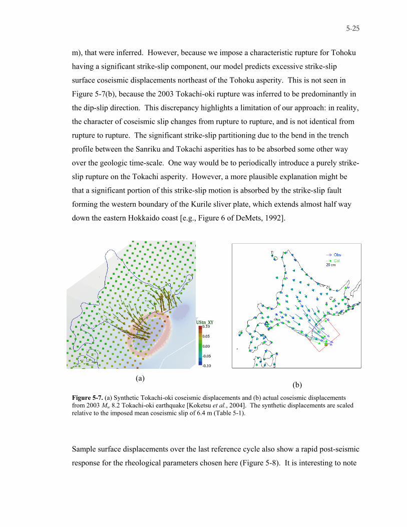
m), that were inferred. However, because we impose a characteristic rupture for Tohoku

having a significant strike-slip component, our model predicts excessive strike-slip

surface coseismic displacements northeast of the Tohoku asperity. This is not seen in

Figure 5-7(b), because the 2003 Tokachi-oki rupture was inferred to be predominantly in

the dip-slip direction. This discrepancy highlights a limitation of our approach: in reality,

the character of coseismic slip changes from rupture to rupture, and is not identical from

rupture to rupture. The significant strike-slip partitioning due to the bend in the trench

profile between the Sanriku and Tokachi asperities has to be absorbed some other way

over the geologic time-scale. One way would be to periodically introduce a purely strike-

slip rupture on the Tokachi asperity. However, a more plausible explanation might be

that a significant portion of this strike-slip motion is absorbed by the strike-slip fault

forming the western boundary of the Kurile sliver plate, which extends almost half way

down the eastern Hokkaido coast [e.g., Figure 6 of DeMets, 1992].

(a)

(b)

Figure 5-7. (a) Synthetic Tokachi-oki coseismic displacements and (b) actual coseismic displacements from 2003 Mw 8.2 Tokachi-oki earthquake [Koketsu et al., 2004]. The synthetic displacements are scaled relative to the imposed mean coseismic slip of 6.4 m (Table 5-1).

Sample surface displacements over the last reference cycle also show a rapid post-seismic

response for the rheological parameters chosen here (Figure 5-8). It is interesting to note

5-26

that both stations displayed here (located along the Sanriku coast) show a different sense

of offset in their north (y) component (middle panels of Figure 5-8) for the 1952 Tokachi-

oki event and the subsequent 1968 Sanriku-oki event. In our synthetic predictions, this is

due to the fact that the applied variable-rake backslip is partitioned into a small northward

component (as opposed to being southward over the rest of the fault surface), over a

small region around the Sanriku asperity (Figure 4-6), because of the change in

orientation of the trench profile relative to the mean plate convergence direction. Such a

reversal is also seen between the 1994 Sanriku-oki and 2003 Tokachi-oki events for this

station. It will be interesting to check whether this latter reversal is indeed observed in

the time-series for this station. A dynamically weaker frictional rheology (smaller α')

could result in a more pronounced post-seismic response than that displayed in Figure

5-8.

Figure 5-8. Sample synthetic surface displacement time-series over the last 75 yr reference cycle for two stations (left: 960533; right: 950156; both located along the Sanriku coast). Blue dashed lines indicate the observed and synthetic GPS velocity estimation window, and the slopes used to infer the velocities are indicated as grey lines within this window.

5-27

Finally, we present comparisons between the GPS velocities estimated for the period

1996–2000 [Hashimoto et al., 2009], and the synthetic velocities assuming both a

frictionless fault, as well as the rate strengthening rheology discussed above. The

observed velocities are relative to the station Adogawa (Geonet #950320), located along

the Japan Sea coast, just off the lower left corners of Figure 5-9 and Figure 5-10. In

contrast, our model predictions are relative to the far-field of the overriding plate (i.e.,

Eurasia). Also, we do not model the incipient subduction thought to be occurring along

the Japan Sea coast. Therefore, our “raw” model predictions near the Japan Sea coastline

are opposite to the above relative velocities. Given that the above reference station is

outside the area we can model with motion purely along the Japan Trench megathrust, we

pick as the reference station, Geonet #950241, which is northeast of Adogawa along the

Japan Sea coast. We confirmed that the observed GPS velocities at this station were

negligible. All synthetic velocities presented below are relative to this station. All

velocities are scaled relative to the plate velocity of 8.3 cm/yr for the Pacific Plate off

Tohoku.

We first compare the predicted horizontal velocity field computed assuming that only the

asperities are locked late in the cycle, and the surrounding fault slips aseismically, at the

long-term slip-rate equal to the plate velocity (Figure 5-9). This scenario is equivalent to

applying backslip over all of the asperities to estimate interseismic velocities. Clearly,

this model explains only a small fraction of the observed horizontal field. From a purely

backslip perspective, areas between the asperities are also required to be “locked”, or

“coupled”, to explain the observed GPS velocities. Alternatively, significant post-

seismic slip in the region between the three southernmost asperities, as well as between

the two northernmost ones, could also explain the misfit.

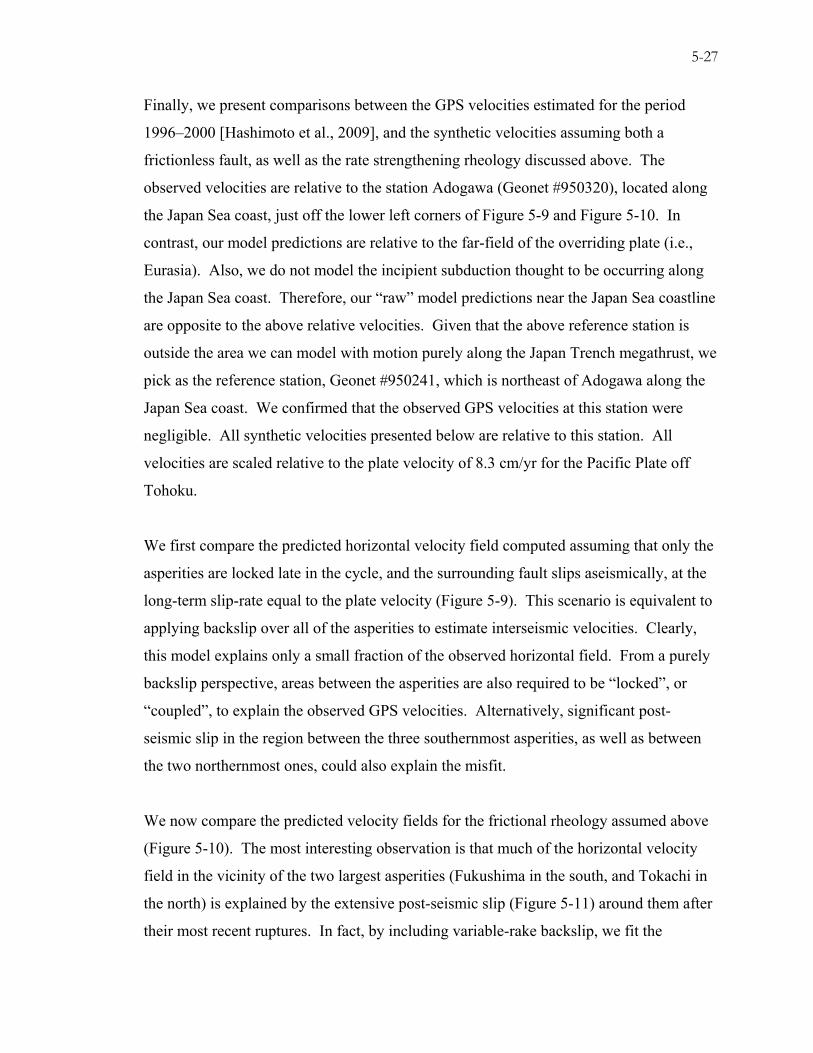
We now compare the predicted velocity fields for the frictional rheology assumed above

(Figure 5-10). The most interesting observation is that much of the horizontal velocity

field in the vicinity of the two largest asperities (Fukushima in the south, and Tokachi in

the north) is explained by the extensive post-seismic slip (Figure 5-11) around them after

their most recent ruptures. In fact, by including variable-rake backslip, we fit the

5-28

Figure 5-9. Observed (left), synthetic-backslip (middle), and residual (right) horizontal GPS velocity fields (relative to a fixed Okhotsk plate) for the period 1996-2000. Synthetics were computed assuming that the fault is locked only at the asperities late in the cycle, and the rest of the fault surface is frictionless. Asperities are shaded in light gray and off-shore of the northern Japan coastline. Thick black arrows indicate the plate convergence direction. Velocities are scaled relative to the plate velocity of 8.3 cm/yr for the Pacific Plate off Tohoku. The color intensity has the same scale in each plot.

Figure 5-10. Observed (left), synthetic-frictional (middle), and residual (right) horizontal GPS velocity fields (relative to a fixed Okhotsk plate) for the period 1996-2000. Synthetics were computed assuming that slip on the fault surface is governed by rate strengthening friction with α' ≈ 1. Asperities are shaded in light gray and off-shore of the northern Japan coastline. Thick black arrows indicate the plate convergence direction. Velocities are scaled relative to the plate velocity of 8.3 cm/yr for the Pacific Plate off Tohoku. The color intensity has the same scale in each plot.

5-29

Figure 5-11. Slip-rates at the end of the cycle, for a fault surface governed by rate strengthening friction with α' ≈ 1. Notice the much larger areas of near-zero slip-rates compared to the upper-left panel of Figure 5-4.

horizontals much better in southern Hokkaido, compared to recently published horizontal

velocity predictions based on a sophisticated inversion scheme that probably did not

include this effect [e.g., Supplementary Figure 1, Hashimoto et al., 2009]. However,

around both these asperities, a dynamically weaker fault (smaller α') would lead to higher

velocities, and perhaps a lower misfit (similar to our conclusion from surface

displacement plots above).

However, there are several regions of significant misfits: (a) northeastern Hokkaido,

along the Nemuro coastline, (b) along the Japan sea coast of southern Hokkaido, (c)

along the eastern coastline of central Tohoku between the Miyagi and Sanriku asperities,

and (d) along the Kanto-sourhern-Tohoku region in central Japan. We now examine each

of these regions more closely.

(a) The biggest residuals are in northeastern Hokkaido, along the Nemuro coastline.

There are a couple of plausible explanations for this discrepancy. The first has to do with

the fact that we have ignored the large 1994 M8.1 Shikotan island earthquake, and

perhaps this asperity needs to be included in our simulation to account for the

discrepancy. The second has to do with the fact that the original slab geometry created in

Gocad has a long-wavelength concave dip starting just downdip of Nemuro asperity. As

5-30

a result, there is considerably less downdip component in the variable rake backslip field

we impose (blue area in the right column of Figure 4-6). This was confirmed by noting

that in the synthetic surface displacement field just prior to the 1973 Nemuro-oki event,

there is a significant trench-parallel, but almost no downdip, component (as would be

expected late in the cycle, landward of a locked patch). So, correcting this long-

wavelength feature (which was missed by the kernel residual checks discussed in Chapter

4) might also help better model the horizontals in this region.

(b) The misfit in southwestern Hokkaido could most likely be from ongoing post-seismic

deformation after the 1993 Mw 7.8 Hokkaido-Nansei-oki earthquake in Japan Sea [Ueda

et al., 2003]. The maximum residuals we obtain for this region are of the order of 0.2 of

the plate velocity, or ~ 1.7 cm/yr. In comparison, the best-fit post-seismic relaxation

models of Ueda et al. [2003] yield horizontal surface velocities of 1.5 and 2 cm/yr.

While there is good agreement between our residuals and their predicted horizontals, we

observe a significant counter-clockwise rotation due to the excess strike-slip component

in the characteristic rupture imposed on the Tokachi asperity as well as the anomalous

strike-slip contribution to the Nemuro asperity (above).

(c) The main characteristic of the misfits in central Tohoku are their trench-perpendicular

orientations. This indicates either (i) that a yet to be detected asperity exists between the

Miyagi and Sanriku asperities [e.g., Slip deficit region in Fig 6 of Miura et al., 2006], or

(ii) this region may be susceptible to episodic aseismic afterslip [Igarashi et al., 2003;

Uchida et al., 2004], or (iii) a region that could become “locked” owing to coseismic

Coulomb stress changes as observed by Miura et al. [2006]. Although many cases of

small but repeating earthquake clusters have also been documented in this region

[Igarashi et al., 2003; Uchida et al., 2004], the frequent release of any accumulated strain

would not result in an apparent slip-deficit along the megathrust interface here, ruling out

the first possibility. Yet another possibility is that the location of the Miyagi asperity

centroid may be too deep. The Japanese coastline in this region is located right above a

steep change in slab dip, and locating the asperity even a little too landward would also

make it deeper, reducing its contribution to the horizontal velocity field.

5-31

(d) Recently, Townsend and Zoback [2006] argued for additional permanent horizontal

deformation in central Japan — beyond that inferred from deformation due to cyclic

subduction zone megathrust ruptures - related to the horizontal motion of the Amurian

plate with respect to northeastern Honshu. Their work was based on Henry et al. [2001],

who estimated net deformation from GPS measurements to be directed west-northwest,

ahead of the Izu-Bonin arc collision. Their inferred direction of additional deformation

and magnitude of approximately 1.5-2 cm/yr agrees reasonably with the misfit in

southern Tohoku.

In spite of the above discrepancies - some of which are due to phenomena we do not

model here – to first order, ruptures on existing asperities do seem to explain a significant

portion of the horizontal velocities in northeastern Japan. Once the Nemuro asperity is

corrected, and the Shikotan rupture is included, we expect the agreement between the

observed and predicted horizontal velocity field to be much better even in northeastern

Hokkaido.

Figure 5-12. Observed (left), synthetic-frictional (middle), and residual (right) vertical GPS velocity fields (relative to a fixed Eurasian plate) for the period 1996-2000, for the same frictional rheology as in Figure 5-10. The observed and predicted vertical velocities as well as their residuals are presented in

Figure 5-12. Deep afterslip seems to explain part of the subsidence along the Sanriku,

and southeastern Hokkaido coasts. However, most of the vertical signal remains

5-32

unexplained. The residuals along the west coast could be due to the fact that we do not

model the incipient subduction in Japan Sea. It has long been known that much of the

eastern Tohoku coastline has been experiencing persistent subsidence relative to the

Eurasian plate. It has been argued that this subsidence is perhaps related to ongoing

subduction erosion [Aoki and Scholz, 2003; Heki, 2004; Hashimoto et al., 2008]. We do

not consider off-fault processes here, and therefore cannot correctly model the observed

vertical geodetic data – even in eastern Tohoku.

5.6 Conclusions and future work

The results presented above demonstrate that the procedure developed here provides us

with a unique way to probe deformation during the late post-seismic to interseismic time-

periods. In a manner similar to the locking of large regions of the megathrust required by

interseismic geodetic data inversions [e.g., Suwa et al., 2006], we too require large areas

of afterslip (especially downdip) of the inferred asperities to explain current horizontal

geodetic velocities. Such large afterslip areas create regions around the asperity having

negligible slip-rates late in the seismic cycle, thus mimicking the effects of large slip-

deficits required by interseismic geodetic data. Explaining the verticals is a more

challenging problem that our single-fault model may not be able to constrain. However,

our hypothesis that mechanical coupling on inferred asperities alone is sufficient to

explain available geodetic observations along the Japan megathrust seems to be

reasonable. More detailed exploration of the frictional rheology parameter space are

required to solidify this assertion. Based on the systematic under-prediction by our

model, we postulate that perhaps a dynamically weaker rheology might be needed to

explain the larger observed late-cycle velocities.

There are some issues related to our model that still need to resolved. Chief among them

is to correct for the slab interface downdip on Nemuro-oki, and add the 1994 Mw 8

Shikotan asperity northeast of the Nemuro asperity. Another issue is the exact plate

convergence velocity used. The values used in literature range from 9.5 cm/yr [e.g.,

5-33

Heki, 2004; Suwa et al., 2006], to 8.3 cm/yr, depending on whether the Eurasian or

Okhotsk plates are used as the reference frame. A 10% larger plate velocity will result in

synthetic velocities being that much larger, and therefore reduce the misfits further in

Fukushima and southeastern Hokkaido. Also, in order to avoid reference frame issues, it

may be more appropriate to compare strain rates instead of velocities. Using depth

dependent rheological parameters may result in slip being constrained to the shallower

portions of the megathrust, leading to stronger horizontal signal from both the shallower

dip (on average) as well as by creating a larger zone of apparent locking.

Looking farther into the future, the procedure introduced here can be extended to model

the full post-seismic to inter-seismic response of the megathrust to specified ruptures.

Including ruptures on other major faults in the region (e.g., those related to incipient

subduction in Japan Sea, or the Kurile sliver) can help us understand the current surface

deformation field even better. This method can also be applied to other subduction zones

where high density geodetic data may become available in the near future (e.g., Sunda

Trench off Sumatra, or the Peru-Chile subduction zone). The ability to probe the

synthetic velocity field in 3D, and being able to follow the evolution of surface

displacements at hundreds of stations simultaneously has potential to provide valuable

insights into the behavior of the subduction zones over the seismic cycle.

5-34

References

Abe, K. (1977), Tectonic implications of the large Shioya-oki earthquakes of 1938, Tectonophysics, 41, 269–289.

ANCORP-Working-Group (2003), Seismic Imaging of a convergent continental margin and plateau in the central Andes (Andean Continental Research Project 1996 (ANCORP'96)), J. Geophys. Res., 108.

Aoki, Y. and C.H. Scholz (2003), Vertical deformation of the Japanese islands, 1996–1999, J. Geophys. Res., 108, 2257, doi:2210.1029/2002JB002129

Bird, P. (2003), An updated digital model of plate boundaries, Geochem Geophy Geosy, 4, 1027, doi:1010.1029/2001GC000252.

Blanpied, M., D. Lockner and D. Byerlee (1991), Fault stability at hydrothermal conditions, Geophys. Res. Lett., 18, 609–612.

Brudzinski, M.R. and W.-P. Chen (2005), Earthquakes and strain in subhorizontal slabs, J. Geophys. Res., 110, B08303.

Buffett, B.A. (2006), Plate force due to bending at subduction zones, J. Geophys. Res., 111, B09405.

Bürgmann, R., M. Kogan, V. Levin, G.E. Hilley, G. Steblov and E. Apel (2005), Interseismic coupling and asperity distribution along the Kamchatka subduction zone, J. Geophys. Res., 110, B07405, doi:07410.01029/02005JB003648.

Chlieh, M., J.-P. Avouac, K. Sieh, D.H. Natawidjaja and J. Galetzka (2008a), Heterogeneous coupling on the Sumatra megathrust constrained from geodetic and paleogeodetic measurements, J. Geophys. Res., 113, B05305.

Chlieh, M., J.P. Avouac, K. Sieh, D.H. Natawidjaja and J. Galetzka (2008b), Heterogeneous coupling of the Sumatran megathrust constrained by geodetic and paleogeodetic measurements, J. Geophys. Res., 113, B05305, doi:05310.01029/02007JB004981

Chlieh, M., J.B.d. Chabalier, J.C. Ruegg, R. Armijo, R. Dmowska, J. Campos and K.L. Feigl (2004), Crustal deformation and fault slip during the seismic cycle in the North Chile subduction zone, from GPS and InSAR observations, Geophys. J. Int., 158, 695-711.

Cisternas, M., B.F. Atwater, F. Torrejn, Y. Sawai, G. Machuca, M. Lagos, A. Eipert, C. Youlton, I. Salgado, T. Kamataki, M. Shishikura, C.P. Rajendran, J.K. Malik, Y. Rizal and M. Husni (2005), Predecessors of the giant 1960 Chile earthquake, Nature, 437, 404-407.

5-35

Cohen, S.C. (1994), Evaluation of the Importance of Model Features For Cyclic Deformation Due to Dip-Slip Faulting, Geophys. J. Int., 119, 831-841.

Cohen, S.C. (1999), Numerical Models of Crustal Deformation in Seismic Zones, Adv. Geophys., 41, 133-231.

Conrad, C.P. and B.H. Hager (1999), Effects of plate bending and fault strength at subduction zones on plate dynamics, J. Geophys. Res., 104, 17551-17571.

DeMets, C. (1992), Oblique Convergence and Deformation Along the Kuril and Japan Trenches, J. Geophys. Res., 97, 17,615–617,625, doi:610.1029/1092JB01306.

DeShon, H.R., S.Y. Schwartz, A.V. Newman, V. González, M. Protti, L.M. Dorman, T.H. Dixon, D.E. Sampson and E.R. Flueh (2006), Seismogenic zone structure beneath the Nicoya Peninsula, Costa Rica, from three-dimensional local earthquake P- and S-wave tomography, Geophys. J. Int., 164, 109–124.

Elsasser, W.M. (1971), Sea-floor spreading as thermal convection, J. Geophys. Res., 76, 1101-1112.

Engdahl, E.R., A. Villasenor, H.R. DeShon and C. Thurber (2007), Teleseismic relocation and assessment of seismicity (1918-2005) in the region of the 2004 Mw 9 Sumatra-Andaman and 2005 M 8.7 Nias great earthquakes, Bull. Seismol. Soc. Am., 97 S43-S61.

Forsyth, D.W. and s. Uyeda (1975), On the relative importance of the driving forces of plate motion, Geophys. J. R. Astron. Soc., 43, 163-200.

Fowler, C.M.R. (1990), The solid earth, edn, vol., Cambridge University Press, Cambridge.

Freund, L.B. and D.M. Barnett (1976), A Two-Dimensional Analysis of Surface Deformation due to Dip-slip Faulting, Bull. Seismol. Soc. Am., 66, 667-675.

Fukahata, Y. and M. Matsu'ura (2006), Quasi-static internal deformation due to a dislocation source in a multilayered elastic/viscoelastic half-space and an equivalence theorem, Geophys. J. Int., 166, 418–434.

Fukuda, J., K. Johnson, K.M. Larson and S. Miyazaki (2009), Friction parameters inferred from the early stages of afterslip following the 2003 Tokachi-oki earthquake, J. Geophys. Res., 114, B04412, doi:04410.01029/02008JB006166.

Gagnon, K., C.D. Chadwell and E. Norabuena (2005), Measuring the onset of locking in the Peru–Chile trench with GPS and acoustic measurements, Nature, 434, 205–208.

Gocad, 2010. (http://www.gocad.org/www/gocad/index.xhtml) Gocad Research Group.

Gutscher, M.-A., W. Spakman, H. Bijwaard and E.R. Engdahl (2000), Geodynamics of at subduction: Seismicity and tomographic constraints from the Andean margin, Tectonics, 19, 814-833.

5-36

Hacker, B.R., S.M. Peacock, G.A. Abers and S.D. Holloway (2003), Subduction Factory, 2: Are intermediate-depth earthquakes in subducting slabs linked to metamorphic dehydration reactions?, J. Geophys. Res., 108, 2030.

Hager, B.H. (1984), Subducted slabs and the geoid: constraints on mantle rheology and flow. , J. Geophys. Res., 89, 6003-6015.

Hamada, N. and Y. Suzuki (2004), Re-examination of aftershocks of the 1952 Tokachi-oki earthquake and a comparison with those of the 2003 Tokachi-oki earthquake, Earth Planets Space, 56, 341–345.

Hashimoto, C., A. Node, T. Sagiya and M. Matsu'ura (2009), Interplate seismogenic zones along the Kuril-Japan trench inferred from GPS data inversion, Nature Geosci., 2, 141-144.

Hashimoto, C., T. Sato and M. Matsu'ura (2008), 3-D simulation of steady plate subduction with tectonic erosion: Current crustal uplift and free-air gravity anomaly in northeast Japan, Pure Appl. Geophys., 165, 567–583, doi:510.1007/s00024-00008-00321-00020.

Heki, K. (2004), Space Geodetic Observation of Deep Basal Subduction Erosion in Northeastern Japan, Earth Planet. Sci. Lett., 219, 13-20.

Henderson, A. (2004), The Paraview Guide, 1st edn, vol., Kitware Inc.

Henry, P., S. Mazzotti and X.L. Pichon (2001), Transient and permanent deformation of central Japan estimated by GPS. 1. Interseismic loading and subduction kinematics, Earth Planet. Sci. Lett., 184, 443-453.

Hetland, E.A. and M. Simons (2010), Postseismic and interseismic deformation due to fault creep II: Transient creep and interseismic stress shadows on megathrusts. , Geophys. J. Int., 181, 99–112, doi:110.1111/j.1365-1246X.2009.04482.x.

Hetland, E.A., M. Simons and E.M. Dunham (2010), Postseismic and interseismic deformation due to fault creep I: Model description, Geophys. J. Int., 181, 81–98, doi:10.1111/j.1365-1246X.2010.04522.x.

Hori, T. (2006), Mechanisms of separation of rupture area and variation in time interval and size of great earthquakes along the Nankai Trough, southwest Japan, J. Earth Simulator, 8-19.

Hsu, Y.-J., M. Simons, J.-P. Avouac, J. Galetzka, K. Sieh, M. Chlieh, D. Natawidjaja, L. Prawirodirdjo and Y. Bock (2006), Frictional Afterslip Following the 2005 Nias-Simeulue Earthquake, Sumatra, Science, 312, 1921-1926.

Hyndman, R.D. and K. Wang (1993), Thermal constraints on the zone of major thrust earthquake failure: The Cascadia subduction zone, J. Geophys. Res., 98, 2039-2060.

5-37

Igarashi, T., T. Matsuzawa and A. Hasegawa (2003), Repeating earthquakes and interplate aseismic slip in the northeastern Japan subduction zone, J. Geophys. Res., 108, 2249, doi:2210.1029/2002JB001920.

Iio, Y., T. Sagiya and Y. Kobayashi (2004), Origin of the Concentrated Deformation Zone in the Japanese Islands and Stress Accumulation Process of Intraplate earthquakes, Earth Planets Space, 56, 831-842.

Iio, Y., T. Sagiya, Y. Kobayashi and I. Shiozaki (2002), Water-weakened lower crust and its role in the concentrated deformation in the Japanese Islands, Earth Planet. Sci. Lett., 203, 245-253.

Ito, A., G. Fujie, T. Tsuru, S. Kodaira, A. Nakanishi and Y. Kaneda (2004), Fault plane geometry in the source region of the 1994 Sanriku-oki earthquake Earth Planet. Sci. Lett., 223, 163-175.

Iwasaki, T., W. Kato, T. Moriya, A. Hasemi, N. Umino, T. Okada, K. Miyashita, T. Mizogami, T. Takeda, S. Seikine, T. Matsushima, K. Tashiro and H. Miyamachi (2001), Extensional structure in northern Honshu arc as inferred from seismic refraction/wide-angle reflection profiling, Geophys. Res. Lett., 28, 2329–2332.

Johnson, K.M., R. Burgmann and K. Larson (2005), Frictional Properties on the San Andreas Fault near Parkfield, California, Inferred from Models of Afterslip following the 2004 Earthquake, Bull. Seism. Soc. Am., 96, S321-338.

Kanamori, H. (1971), Focal mechanism of the Tokachi-Oki earthquake of may 16, 1968: Contortion of the lithosphere at a junction of two trenches, Tectonophysics, 12, 1-13.

Kanamori, H. and D.L. Anderson (1975), Theoretical basis of some empirical relations in seismology, Bull. Seism. Soc. Am., 65, 1073-1095.

Kanda, R.V.S. and M. Simons (2010), An elastic plate model for interseismic deformation in subduction zones, J. Geophys. Res., 115, B03405.

Kato, N. (2008), Numerical simulation of recurrence of asperity rupture in the Sanriku region, northeastern Japan, J. Geophys. Res., 113, B06302, doi:06310.01029/02007JB005515.

Khazaradze, G. and J. Klotz (2003), Short and long-term effects of GPS measured crustal deformation rates along the South-Central Andes, J. Geophys. Res., 108, 2289.

Klotz, J., A. Abolghasem, G. Khazaradze, B. Heinze, T. Vietor, R. Hackney, K. Bataille, R. Maturana, J. Viramonte and R. Perdomo, 2006. Long-term signals in the present-day deformation field of the Central and Southern Andes and Constraints on the viscosity of the Earth's Upper Mantle. . in The Andes: Active Subduction Orogeny, Frontiers in Earth Sciences, pp. 65–89, eds Oncken, O., Chong, G., Franz, G., Giese, P., Goetze, H., Ramos, V. A., Strecker, M. R.andWigger, P. Springer Berlin.

5-38

Koketsu, K., K. Hikima, S. Miyazaki and S. Ide (2004), Joint inversion of strong motion and geodetic data for the source process of the 2003 Tokachi-oki, Hokkaido, earthquake, Earth Planets Space, 56, 329–334.

Konca, A.O., J.P. Avouac, A. Sladen, A.J. Meltzner, K. Sieh, P. Fang, Z.H. Li, J. Galetzka, J. Genrich, M. Chlieh, D.H. Natawidjaja, Y. Bock, E.J. Fielding, C. Ji and D.V. Helmberger (2009), Partial rupture of a locked patch of the Sumatra megathrust during the 2007 earthquake sequence, Nature, 456, 631-635.

Lapusta, N. and J. Rice (2003), Nucleation and early seismic propagation of small and large events in a crustal earthquake model, J. Geophys. Res., 108, 2205, doi:2210.1029/2001JB000793.

Larson, K., P. Bodin and J. Gomberg (2003), Using 1 Hz GPS Data to Measure Permanent and Seismic Deformations Caused by the Denali Fault Earthquake, Science, 300, 1421-1424.

Loveless, J.P. and B.J. Meade (2010), Geodetic imaging of plate motions, slip rates, and partitioning of deformation in Japan, J. Geophys. Res., 115, B02410, doi:02410.01029/02008JB006248.

Marone, C., C. Scholz and R. Bilham (1991), On the mechanics of earthquake afterslip, J. geophys. Res., 96, 8441–8452.

Massonnet, D. and K.L. Feigl (1998), Radar interferometry and its application to changes in the earth's surface, Reviews Geophys., 36, 441-500

Masterlark, T. (2003), Finite element model predictions of static deformation from dislocation sources in a subduction zone: Sensitivities to homogeneous, isotropic, Poisson-solid, and half-space assumptions, J. Geophys. Res., 108 2540.

Matsu'ura, M. and T. Sato (1989), A dislocation model for the earthquake cycle at convergent plate boundaries, Geophys. J. Int., 96, 23-32.

Meade, B.J. (2007), Algorithms for the calculation of exact displacements, strains, and stresses for triangular dislocation elements in a uniform elastic half space. , Comp. Geosci., 33, 1064-1075, doi:1010.1016/j.cageo.2006.1012.1003.

Miura, S., I. Iinuma, S. Yui, N. Uchida, T. Sato, K. Tachibana and A. Hasegawa (2006), Co- and post-seismic slip associated with the 2005 Miyagi-oki earthquake (M7.2) as inferred from GPS data, Earth Planets Space, 58, 1567–1572.

Miura, S., S. Kodaira, A. Nakanishi and T. Tsuru (2003), Structural characteristics controlling the seismicity of southern Japan Trench fore- arc region, revealed by ocean bottom seismographic data, Tectonophysics, 363, 79-102.

Miura, S., N. Takahashi, A. Nakanishi, T. Tsuru, S. Kodaira and Y. Kaneda (2005), Structural characteristics off Miyagi forearc region, the Japan Trench seismogenic zone, deduced from a wide-angle reflection and refraction study, Tectonophysics, 407, 165-188.

5-39

Miyazaki, S., P. Segall, J. Fukuda and T. Kato, 2004. Space time distribution of afterslip following the 2003 Tokachi-oki earthquake: Implications for variations in fault zone frictional properties. in Geophys. Res. Lett., pp. L06623.

Nakanishi, A., A.J. Smith, S. Miura, T. Tsuru, S. Kodaira, K. Obana, N. Takahashi, P.R. Cummins and Y. Kaneda (2004), Structural factors controlling the coseismic rupture zone of the 1973 Nemuro-Oki earthquake, the southern Kuril Trench seismogenic zone, J. Geophys. Res., 109, B05305, doi: 05310.01029/02003JB002574.

Nakayama, W. and M. Takeo (1997), Slip history of the 1994 Sanriku-Haruka-Oki, Japan, earthquake deduced from strong-motion data, B. Seismol. Soc. Am., 87, 918-931.

Nanayama, F., K. Satake, R. Furukawa, K. Shimokawa, B.F. Atwater, K. Shigeno and S. Yamaki (2003), Unusually large earthquakes inferred from tsunami deposits along the Kuril trench, Nature, 424, 660–663.

Nishimura, T., T. Hirasawa, S. Miyazaki, T. Sagiya, T. Tada, S. Miura and K. Tanaka (2004), Temporal change of interplate coupling in northeastern Japan during 1995-2002 estimated from continuous GPS observations, Geophys. J. Int., 157, 901-916.

Nishimura, T., H. Nakahara, H. Sato and M. Ohtake (1996), Source process of the 1994 far east off Sanriku earthquake, Japan, as inferred from a broad-band seismogram, Tohoku Geophys. J., 34, 121−134.

Okada, Y. (1992), Internal deformation due to shear and tensile faults in a half-space, Bull. Seismol. Soc. Am., 82, 1018-1040.

Oleskevich, D.A., R.D. Hyndman and K. Wang (1999), The updip and downdip limits to great subduction earthquakes: thermal and structural models of Cascadia, south Alaska, SW Japan, and Chile, J. Geophys. Res., 104, 14965–14991.

Owen, S.J., 2006. CUBIT 10.2 Documentation, pp. 532, Sandia National Laboratories, Albuquerque, NM, U.S.A.

Park, J.-O., T. Tsuru, S. Kodaira, P.R. Cummins and Y. Kaneda (2002), Splay Fault Branching Along the Nankai Subduction Zone, Science, 297, 1157-1160.

Perfettini, H. and J.-P. Ampuero (2008), Dynamics of a velocity strenghtening region: implications for slow earthquakes and postseismic slip, J. Geophys. Res., 113, B09411, doi:09410.01029/02007JB005398.

Perfettini, H. and J. Avouac (2004), Postseismic relaxation driven by brittle creep: A possible mechanism to reconcile geodetic measurements and the decay rate of aftershocks, application to the Chi-Chi earthquake, Taiwan, J. Geophys. Res., 109, B02304.

Perfettini, H. and J.P. Avouac (2007), Modeling afterslip and aftershocks following the 1992 Landers earthquake, J. Geophys. Res., 112, B07409, doi: 07410.01029/02006JB004399.

5-40

Rani, S. and S.J. Singh (1992), Static Deformation of a Uniform Half-space due to a Long Dip-slip Fault, Geophys. J. Int., 109, 469-476.

Rice, J. (1993), Spatio-temporal complexity of slip on a fault, J. geophys. Res. , 98, 9885–9907.

Robinson, D.P. and L.T. Cheung (2003), Source process of the Mw 8.3, 2003 Tokachi-Oki, Japan earthquake and its aftershocks, Geoph. J. Intl., 181, 334-342, DOI: 310.1111/j.1365-1246X.2010.04513.x.

Ruff, L.J. (1992), Asperity distributions and large earthquake occurrence in subduction zones, Tectonophysics, 211, 61-83.

Rundle, J.B. (1982), Viscoelastic-gravitational deformation by a rectangular thrust fault in a layered Earth, J. Geophys. Res., 87, 7787-7796.

Satake, K. and B.F. Atwater (2007), Long-term perspectives on giant earthquakes and tsunamis at subduction zones, Annu. Rev. Earth Planet Sci., 35, 349-274.

Satake, K., K. Hirata, S. Yamaki and Y. Tanioka (2006), Re-estimation of tsunami source of the 1952 Tokachi-oki earthquake, Earth, Planets and Space, 58, 535-542.

Sato, T. and M. Matsu'ura (1988), A kinematic model for deformation of the lithosphere at subduction zones, J. Geophys. Res., 93, 6410–6418.

Sato, T. and M. Matsu'ura (1992), Cyclic crustal movement, steady uplift of marine terraces, and evolution of the island arc-trench system in southwest Japan, Geophys. J. Int., 111, 617–629.

Sato, T. and M. Matsu'ura (1993), A kinematic model for evolution of island arc-trench systems, Geophys. J. Int., 114, 512-530.

Savage, J.C. (1983), A dislocation model of strain accumulation and release at a subduction zone, J. Geophys. Res., 88 4984-4996.

Savage, J.C. (1995), Interseismic uplift at the Nankai subduction zone, Southwest Japan, 1951–1990, J. Geophys. Res., 100, 6339–6350.

Savage, J.C. (1996), Comment on "The stress state implied by dislocation models of subduction deformation" by J. J. Douglass and B. A. Buffett, Geophys. Res. Lett., 23, 2709-2710.

Savage, J.C. (1998), Displacement field for an edge dislocation in a layered half-space, J. Geophys. Res., 103, 2439-2446.

Scholz, C.H. (1990), The Mechanics of Earthquakes and Faulting, edn, vol., pp. 439, Cambridge University Press, New York.

Schroeder, W., K. Martin and B. Lorensen (2006), The Visualization Toolkit An Object-Oriented Approach To 3D Graphics, 4th edn, vol., Kitware Inc. .

5-41

Seno, T., K. Shimazaki, P. Somerville, K. Sudo and T. Eguchi (1980), Rupture process of the Miyagi-oki, Japan, earthquake of June 12, 1978, Phys. Earth Planet. Int., 23, 39-61.

Seth, B.R. (1935), Finite Strain in Elastic Problems, Philosophical Transactions of the Royal Society of London, 234, 231-264.

Shimazaki, K. (1974), Nemuro-Oki earthquake of June 17, 1973: A lithospheric rebound at the upper half of the interface, Phys. Earth. Planet. In., 9, 314-327.

Shimazaki, K. and T. Nakata (1980), Time-predictable recurrence model for large earthquakes, Geophys. Res. Lett., 7, 279–282.

Sieh, K., D.H. Natawidjaja, A.J. Meltzner, C.-C. Shen, H. Cheng, K.-S. Li, B.W. Suwargadi, J.G. Philibosian and R.L. Edwards (2008), Earthquake supercycles inferred from sea-level changes recorded in the corals of West Sumatra, Science, 322, 1674-1678, doi:1610.1126/science.1163589.

Sieh, K., S.N. Ward, D. Natawidjaja and B.W. Suwargadi (1999), Crustal deformation at the Sumatran subduction zone revealed by coral rings, Geophys. Res. Lett., 26, 3141-3144.

Simoes, M., J.-P. Avouac, R. Cattin and P. Henry (2004), The Sumatra Subduction Zone: A Case for a Locked Fault Zone Extending into the Mantle, J. Geophys. Res., 109, B10402.

Simons, M. and P. Rosen, 2007. Interferometric Synthetic Aperture Radar Geodesy. in Treatise on Geophysics, pp. 391-446, ed Schubert, G. Elsevier Press.

Souter, B.J. and B.H. Hager (1997), Fault propagation fold growth during the 1994 Northridge, California, earthquake?, J. Geophys. Res., 102, 11,931–911,942.

Subarya, C., M. Chlieh, L. Prawirodirdjo, J.P. Avouac, Y. Bock, K. Sieh, A. Meltzner, D. Natawidjaja and R. McCaffrey (2006), Plate-boundary deformation of the great Aceh-Andaman earthquake, Nature, 440, 46–51.

Suppe, J. (1985), Principles of Structural Geology, edn, vol., Prentice-Hall.

Suwa, Y., S. Miura, A. Hasegawa, T. Sato and K. Tachibana (2006), Interplate coupling beneath NE Japan inferred from three-dimensional displacement field, J. Geophys. Res., 111, B04402.

Takahashi, N., S. Kodaira, T. Tsuru, J.-O. Park, Y. Kaneda, K. Suyehiro, H. Kinoshita, S. Abe, M. Nishino and R. Hino (2004), Seismic structure and seismogenesis off Sanriku region, northeastern Japan, Geophys. J. Int., 159, 129-145.

Tanioka, Y., 2003a. Rupture area of the 1894 Nemuro-oki earthquake is larger than that of the 1973 Nemurooki earthquake. in Japan Geoscience Union Meeting, s208-007, pp. Abstract s208-007.

5-42

Tanioka, Y., 2003b. Source processes of the 1936 and 1978 Miyagi-oki earthquakes from the tsunami waveform analysis. in Japan Geoscience Union Meeting, s052-002, pp. Abstract s052-002.

Tanioka, Y., L. Ruff and K. Satake (1996), The Sanriku-Oki, Japan, Earthquake of December 28, 1994 (Mw 7.7): Rupture of a different asperity from a previous earthquake, Geophys. Res. Lett., 23, 1465–1468.

Thatcher, W. and J.B. Rundle (1979), A model for the earthquake cycle in underthrust zones, J. Geophys. Res., 84, 5540-5556.

Thatcher, W. and J.B. Rundle (1984), A viscoelastic coupling model for the cyclic deformation due to periodically repeated earthquakes at subduction zones, J. Geophys. Res., 89, 7631-7640.

Tomar, S. and N.K. Dhiman (2003), 2-D Deformation Analysis of a Half-space due to a Long Dip-slip Fault at Finite Depth, Proc. Indian Acad. Sci. (Earth Planet. Sci.), 112, 587-596.

Townsend, J. and M.D. Zoback (2006), Stress, strain, and mountain building in central Japan, J. Geophys. Res., 111, B03411, doi:03410.01029/02005JB003759.

Turcotte, D.L. and G. Schubert (2001), Geodynamics, 2 edn, vol., Cambridge University Press, New York.

Twiss, R.J. and E.M. Moores (1992), Structural Geology, 1st edn, vol., W. H. Freeman and Company, New York.

Uchida, N., A. Hasegawa, T. Matsuzawa and T. Igarashi (2004), Pre- and post-seismic slip on the plate boundary off Sanriku, NE Japan associated with three interplate earthquakes as estimated from small repeating earthquake data, Tectonophys, 385, 1–15.

Ueda, H., M. Ohtake and H. Sato (2003), Postseismic crustal deformation following the 1993 Hokkaido Nansei-oki earthquake, northern Japan: Evidence for a low-viscosity zone in the uppermost mantle, J. Geophys. Res., 108, 2151, doi:2110.1029/2002JB002067.

Umino, N., T. Kono, T. Okada, J. Nakajima, T. Matsuzawa, N. Uchida, H. A., Y. Tamura and G. Aoki (2006), Revisiting the three Mw7 Miyagioki earthquakes in the 1930s: possible seismogenic slip on asperities that were re-ruptured during the 1978 M=7.4 Miyagi-oki earthquake, Earth Planets Space, 58, 1587-1592.

Vergne, J., R. Cattin and J.P. Avouac (2001), On the use of Dislocations to Model Interseismic Strain and Stress Build-up at Intracontinental Thrust Faults, Geophys. J. Int., 147, 155-162.

Wang, K. (2007), Elastic and viscoelastic models of crustal deformation in subduction earthquake cycles. in The Seismogenic Zone of Subduction Thrust Faults, eds. Dixon, T.andMoore, J. C., pp. 540-575, Columbia University Press, New York.

5-43

Wang, K. and Y. Hu (2006), Accretionary Prisms in Subduction Earthquake Cycles: The Theory of Dynamic Coulomb Wedge, J. Geophys. Res., 111, B06410.

Wang, K., R. Wells, S. Mazzotti, R.D. Hyndman and T. Sagiya (2003), A revised dislocation model of interseismic deformation of the Cascadia subduction zone, J. Geophys. Res., 108, 2026.

Wang, R. (2005), The dislocation theory: a consistent way for including the gravity effect in (visco)elastic plane-earth models, Geophys. J. Int., 161, 191-196.

Williams, C.A. and R. McCaffrey (2001), Stress rates in the central Cascadia subduction zone inferred from an elastic plate model, Geophys. Res. Lett., 28, 2125-2128.

Yamanaka, Y. and M. Kikuchi (2003), Source processes of the recurrent Tokachi-oki earthquake on September 26, 2003, inferred from teleseismic body waves, Earth Planet. Sci. Lett., 55, e21– e24.

Yamanaka, Y. and M. Kikuchi (2004), Asperity map along the subduction zone in northeastern Japan inferred from regional seismic data, J. Geophys. Res., 109, B07307, doi:07310.01029/02003JB002683.

Yoshioka, S., T. Yabuki, T. Sagiya, T. Tada and M. Matsu'ura (1993), Interplate coupling and relative plate motion in the Tokai district, central Japan, deduced from geodetic data inversion using ABIC, Geophys. J. Int., 113, 607-621.

Zhao, S. and S. Takemoto (2000), Deformation and stress change associated with plate interaction at subduction zones: a kinematic modeling, Geophys. J. Int., 142, 300-318.

Zweck, C., J.T. Freymueller and S.C. Cohen (2002), Three-dimensional elastic dislocation modeling of the postseismic response to the 1964 Alaska earthquake, J. Geophys. Res., 107, 2064.