Chapter 5: Color and Blending

This chapter discusses color issues in computer graphics from first principles. We introduce theRGB model for specifying color, the most common model for digital color work, along with theconcept of luminance for color to permit persons with color vision deficiencies to get the sameinformation that the color was intended to provide. We discuss two other color models, HLS andHSV, which are sometimes useful for color specification, and give the conversion functions fromthese models to RGB. We give the RGBA extension to the RGB model that permits colorblending and show how that can be used to simulate transparency, and we introduce the use ofcolor anaglyphs as a color-based 3D viewing. We then show how color is implemented forOpenGL graphics programming. When you have finished with this chapter, you should be able toinclude color in your graphics programming to make it much more interesting and informative.

Introduction

Color is a fundamental concept for computer graphics. We need to be able to define colors for ourgraphics that represent good approximations of real-world colors, and we need to be able tomanipulate colors as we develop our applications.

There are many ways to specify colors, but all depend principally on the fact that the human visualsystem generally responds to colors through the use of three kinds of cells in the retina of the eye.This response is complex and includes both physical and psychological processes, but thefundamental fact of three kinds of stimulus is maintained by all the color models in computergraphics. For most work, the usual model is the RGB (Red, Green, Blue) color model thatmatches in software the physical design of computer monitors, which are made with a pattern ofthree kinds of phosphor which emit red, green, and blue light when they are excited by an electronbeam. This RGB model is used for color specification in almost all computer graphics APIs, and itis the basis for the discussion here. There are a number of other models of color, and we discuss afew of these in this chapter. However, we refer you to textbooks and other sources, especiallyFoley et al. [FvD], for additional discussions on color models and for more complete informationon converting color representations from one model to another.

Because the computer monitor uses three kinds of phosphor, and each phosphor emits light levelsbased on the energy of the electron beam that is directed at it, a common approach is to specify acolor by the level of each of the three primaries. These levels are a proportion of the maximum lightenergy that is available for that primary, so an RGB color is specified by a triple (r, g, b) whereeach of the three components represents the amount of that particular component in the color andwhere the ordering is the red-green-blue that is implicit in the name RGB. Colors can be specifiedin a number of ways in the RGB system, but in this book we will specify each component by theproportion of the maximum intensity we want for the color. This proportion for each primary isrepresented by a real number between 0.0 and 1.0, inclusive. There are other ways to representcolors, of course. In an integer-based system that is also often used, each color component can berepresented by an integer that depends on the color depth available for the system; if you have eightbits of color for each component, which is a common property, the integer values are in the range 0to 255. The real-number approach is used more commonly in graphics APIs because it is moredevice-independent. In either case, the number represents the proportion of the available color ofthat primary hue that is desired for the pixel. Thus the higher the number for a component, thebrighter is the light in that color, so with the real-number representation, black is represented by(0.0, 0.0, 0.0) and white by (1.0, 1.0, 1.0). The RGB primaries are represented respectively byred (1.0, 0.0, 0.0), green (0.0, 1.0, 0.0), and blue (0.0, 0.0, 1.0); that is, colors that are fullybright in a single primary component and totally dark in the other primaries. Other colors are a mixof the three primaries as needed.

2/18/03 Page 5.2

While we say that the real-number representation for color is more device-independent, mostgraphics hardware deals with colors using integers. Floating-point values are converted to integersto save space and to speed operations, with the exact representation and storage of the integersdepending on the number of bits per color per pixel and on other hardware design issues. Thisdistinction sometimes comes up in considering details of color operations in your API, but isgenerally something that you can ignore. Some color systems outside the usual graphics APIs usespecial kinds of color capabilities and there are additional technologies for representing and creatingthese capabilities. However, the basic concept of using floating-point values for colors is the sameas for our APIs. The color-generation process itself is surprisingly complex because the monitoror other viewing device must generate perceptually-linear values, but most hardware generatescolor with exponential, not linear, properties. All these color issues are hidden from the APIprogrammer, however, and are managed after being translated from the API representations of thecolors, allowing API-based programs to work relatively the same across a wide range ofplatforms.

In addition to dealing with the color of light, modern graphics systems add a fourth component tothe question of color. This fourth component is called “the alpha channel” because that was itsoriginal notation [POR], and it represents the opacity of the material that is being modeled. As isthe case with color, this is represented by a real number between 0.0 (no opacity — completelytransparent) and 1.0 (completely opaque — no transparency). This is used to allow you to createobjects that you can see through at some level, and can be a very valuable tool when you want tobe able to see more than just the things at the front of a scene. However, transparency is notdetermined globally by the graphics API; it is determined by compositing the new object withwhatever is already present in the Z-buffer. Thus if you want to create an image that contains manylevels of transparency, you will need to pay careful attention to the sequence in which you drawyour objects, drawing the furthest first in order to get correct attenuation of the colors ofbackground objects.

Principles

Specifying colors for geometry

The basic principle for using color with graphics is simple: once you have specified a color, all thegeometry that is specified after that point will be drawn in the specified color until that color ischanged. This means that if you want different parts of your scene to be presented in differentcolors you will need to re-specify the color for each distinct part, but this is not difficult.

In terms of the scene graph, color is part of the appearance node that accompanies each geometrynode. We will later see much more complex ways to determine an appearance, but for now coloris our first appearance issue. When you write your code from the scene graph, you will need towrite the code that manages the appearance before you write the code for the geometry in order tohave the correct appearance information in the system before the geometry is drawn.

Color may be represented in the appearance node in any way you wish. Below we will discussthree different kinds of color models, and in principle you may represent color with any of these.However, most graphics APIs support RGB color, so you may have to convert your colorspecifications to RGB before you can write the appearance code. Later in this chapter we includecode to do two such conversions.

The RGB cube

The RGB color model is associated with a geometric presentation of a color space. That space canbe represented by a cube consisting of all points (r, g, b) with each of r, g, and b having a valuethat is a real number between 0 and 1. Because of the easy analogy between color triples and space

2/18/03 Page 5.3

triples, every point in the unit cube can be easily identified with a RGB triple representation of acolor. This gives rise to the notion of the RGB color cube, a 3D space whose coordinates are eachbounded by 0 and 1 and with each point associated with a color. The color is, of course, the colorwhose red, green, and blue values are the r, g, and b coordinates of the point. This identificationis very natural and most people in computer graphics think of the color space and the color cubeinterchangeably.

To illustrate the numeric properties of the RGB color system, we will create the edges of the colorcube as shown in Figure 5.1 below, which has been rotated to illustrate the colors more fully. Todo this, we create a small cube with a single color, and then draw a number of these cubes aroundthe edge of the geometric unit cube, with each small cube having a color that matches its location.We see the origin (0,0,0) corner, farthest from the viewer, mostly by its absence because of theblack background, and the (1,1,1) corner nearest the viewer as white. The three axis directions arethe pure red, green, and blue corners. Creating this figure is discussed below in the section on

Figure 5.1: tracing the colors of the edges of the RGB cube

creating a model with a full spectrum of colors, and it would be useful to add an interior cubewithin the figure shown that could be moved around the space interactively and would changecolor to illustrate the color at its current position in the cube.

This figure suggests the nature of the RGB cube, but a the entire RGB cube is much morecomplete. It shown from two points of view in Figure 5.2, from the white vertex and from theblack vertex, so you can see the full range of colors on the surface of the cube. Note that the threevertices closest to the white vertex are the cyan, magenta, and yellow vertices, while the threevertices closest to the black vertex are the red, green, and blue vertices. This illustrates the additivenature of the RGB color model, with the colors getting lighter as the amounts of the primary colors

Figure 5.2: two views of the RGB cube — from the white (left) and black (right) corners

2/18/03 Page 5.4

increase, as well as the subtractive nature of the CMY color model, where the colors get darker asthe amounts of color increase. This will be explored later and will be contrasted to the subtractivenature of other color models. Of course, all points interior to the cube also correspond to colors.For example, the center diagonal of the RGB cube from (0, 0, 0) to (1, 1, 1) corresponds to thecolors with equal amounts of each primary; these are the gray colors that provide the neutralbackgrounds that are very useful in presenting colorful images.

Color is extremely important in computer graphics, and we can get color in our image in two ways:by directly setting the color for the objects we are drawing, or by defining properties of objectsurfaces and lights and having the color generated by a lighting model. In this chapter we onlythink about the colors of objects, and save the color of lights and the way light interacts withsurfaces for a later chapter on lighting and shading. In general, the behavior of a scene will reflectboth these attributes—if you have a red object and illuminate it with a blue light, your object willseem to be essentially black, because a red object reflects no blue light and the light contains noother color than blue.

Luminance

Luminance of a color is the color’s brightness, or the intensity of the light it represents, withoutregard for its actual color. This concept is particularly meaningful for emissive colors on thescreen, because these actually correspond to the amount of light that is emitted from the screen.The concept of luminance is important for several reasons. One is that a number of members ofany population have deficiencies in the ability to distinguish different colors, the family of so-calledcolor blindness problems, but are able to distinguish differences in luminance. You need to takeluminance into account when you design your displays so that these persons can make sense ofthem Luminance is also important because part of the interpretation of an image deals with thebrightness of its parts, and you need to understand how to be sure that you use colors with theright kind of luminance for your communication. Fore example, in the chapter on visualcommunication we will see how we can use luminance information to get color scales that areapproximately uniform in terms of having the luminance of the color represent the numerical valuethat the color is to represent.

For RGB images, luminance is quite easy to compute. Of the three primaries, green is thebrightest and so contributes most to the luminance of a color. Red is the next brightest, and blue isthe least bright. The actual luminance will vary from system to system and even from displaydevice to display device because of differences in the way color numbers are translated intovoltages and because of the way the phosphors respond. In general, though, we are relativelyaccurate if we assume that luminance is calculated by the formula

luminance = 0.30*red + 0.59 * green 0.11*blueso the overall brightness ratios are approximately 6:3:1 for green:red:blue.

To see the effects of constant luminance, we can pass a plane 0.30R+0.59G+0.11B+t through theRGB color space and examine the plane it exposes in the color cube as the parameter t varies. Anexample of this is shown in Figure 5.3 in both color and grayscale.

2/18/03 Page 5.5

Figure 5.3: a plane of constant luminance in the RGB cube in both color (left) and gray (right)

Other color models

There are times when the RGB color model is not easy or natural to use. When we want to capturea particular color, few of us think of the color in terms of the proportions of red, green, and bluethat are needed to create it. Other color models give us different ways to think about color thatmake it more intuitive to specify a color. There are also some processes for which the RGBapproach does not model the reality of color production. We need to have a wider range of waysto model color to accomodate these realities.

A more intuitive approach to color is found with two other color models: the HSV (Hue-Saturation-Value) and HLS (Hue-Lightness-Saturation) models. These models represent color as ahue (intuitively, a descriptive variation on a standard color such as red, or magenta, or blue, orcyan, or green, or yellow) that is modified by setting its value (a property of the color’s darknessor lightness) and its saturation (a property of the color’s vividness). This lets us find numericalways to say “the color should be a dark, vivid reddish-orange” by using a hue that is to the red sideof yellow, has a relatively low value, and has a high saturation.

Just as there is a geometric model for RGB color space, there is one for HSV color space: a conewith a flat top, as shown in Figure 5.4 below. The distance around the circle in degrees representsthe hue, starting with red at 0, moving to green at 120, and blue at 240. The distance from thevertical axis to the outside edge represents the saturation, or the amount of the primary colors in theparticular color. This varies from 0 at the center (no saturation, which makes no real coloring) to 1at the edge (fully saturated colors). The vertical axis represents the value, from 0 at the bottom (nocolor, or black) to 1 at the top. So a HSV color is a triple representing a point in or on the cone,and the “dark, vivid reddish-orange” color would be something like (40.0, 1.0, 0.7). Code todisplay this geometry interactively is discussed at the end of this chapter, and writing an interactivedisplay program gives a much better view of the space.

Figure 5.4: three views of HSV color space: side (left), top (middle), bottom (right)

The shape of the HSV model space can be a bit confusing. The top surface represents all thelighter colors based on the primaries, because colors getting lighter have the same behavior ascolors becoming less saturated. The reason the geometric model tapers to a point at the bottom isthat there is no real color variation near black. In this model, the gray colors are the colors with a

2/18/03 Page 5.6

saturation of 0, which form the vertical center line of the cone. For such colors, the hue ismeaningless, but it still must be included.

In the HLS color model, shown in Figure 5.5, the geometry is much the same as the HSV modelbut the top surface is stretched into a second cone. Hue and saturation have the same meaning asHSV but lightness replaces value, and lightness corresponds to the brightest colors at a value of0.5. The rationale for the dual cone that tapers to a point at the top as well as the bottom is that ascolors get lighter, they lose their distinctions of hue and saturation in a way that is very analogouswith the way colors behave as they get darker. In some ways, the HLS model seems to comecloser to the way people talk about “tints” and “tones” when they talk about paints, with thestrongest colors at lightness 0.5 and becoming lighter (tints) as the lightness is increased towards1.0, and becoming darker (tones) as the lightness is decreased towards 0.0. Just as in the HSVcase above, the grays form the center line of the cone with saturation 0, and the hue ismeaningless.

Figure 5.5: the HLS double cone from the red (left), green (middle), and blue(right) directions.

The top and bottom views of the HLS double cone look just like those of the HSV single cone, butthe side views of the HLS double cone are quite different. Figure 5.5 shows the HLS double conefrom the three primary-color sides: red, green, and blue respectively. The views from the top orbottom are exactly those of the HSV cone and so are now shown here. The images in the figure donot show the geometric shape very well; the discussion of this model in the code section below willshow you how this can be presented, and an interactive program to display this space will allowyou to interact with the model and see it more effectively in 3-space.

There are relatively simple functions that convert a color defined in one space into the same color asdefined in another space. We do not include all these functions in these notes, but they are coveredin [FvD], and the functions to convert HSV to RGB and to convert HLS to RGB are included inthe code discussions below about producing these figures.

All the color models above are based on colors presented on a computer monitor or other devicewhere light is emitted to the eye. Such colors are called emissive colors, and operate by addinglight at different wavelengths as different screen cells emit light. The fact that most color presentedby programming comes from a screen makes this the primary way we think about color incomputer graphics systems. This is not the only way that color is presented to us, however.When you read these pages in print, and not on a screen, the colors you see are generated by lightthat is reflected from the paper through the inks on the page. Such colors can be calledtransmissive colors and operate by subtracting colors from the light being reflected from the page.This is a totally different process and needs separate treatment. Figure 5.6 illustrates this principle.

2/18/03 Page 5.7

The way the RGB add to produce CMY and eventually white shows why emissive colors aresometimes called additive colors, while the way CMY produce RGB and eventually black showswhy transmissive colors are sometimes called subtractive colors.

Figure 5.6: emissive colors (left) and transmissive colors (right)

Transmissive color processes use inks or films that transmit only certain colors while filtering outall others. Two examples are the primary inks for printing and the films for theater lights; theprimary values for transmissive color are cyan (which transmits both blue and green), magenta(which transmits both blue and red), and yellow (which transmits both red and green). Inprinciple, if you use all three inks or filters (cyan, magenta, and yellow), you should have no lighttransmitted and so you should see only black. In practice, actual materials are not perfect andallow a little off-color light to pass, so this would produce a dark and muddy gray (the thing thatprinters call “process black”) so you need to add an extra “real” black to the parts that are intendedto be really black. This cyan-magenta-yellow-black model is called CMYK color and is the basisfor printing and other transmissive processes. It is used to create color separations that combine toform full-color images as shown in Figure 5.7, which shows a full-color image (left) and the setsof yellow, cyan, black, and magenta separations (right-hand side, clockwise from top left) that areused to create plates to print the color image. We will not consider the CMYK model further in thisdiscussion because its use is in printing and similar technologies, but not in graphicsprogramming. We will meet this approach to color again when we discuss graphics hardcopy,however.

Figure 5.7: color separations for printing

2/18/03 Page 5.8

Color depth

The numerical color models we have discussed above are device-independent; they assume thatcolors are represented by real numbers and thus that there are an infinite number of colors availableto be displayed. This is, of course, an incorrect assumption, because computers lack the capabilityof any kind of infinite storage. Instead, computers use color capabilities based on the amount ofmemory allocated to holding color information.

The basic model we usually adopt for computer graphics is based on screen displays and can becalled direct color. For each pixel on the screen we store the color information directly in thescreen buffer. The number of bits of storage we use for each color primary is called the colordepth for our graphics. At the time of this writing, it is probably most common to use eight bits ofcolor for each of the R, G, and B primaries, so we often talk about 24-bit color. In fact, it is notuncommon to include the Z-buffer depth in the color discussion, with the model of RGBA color,and if the system uses an 8-bit Z-buffer we might hear that it has 32-bit color. This is notuniversal, however; some systems use fewer bits to store colors, and not all systems use an equalnumber of bits for each color, while some systems use more bits per color. The very highest-endprofessional graphics systems, for example, often use 36-bit or 48-bit color. However, someimage formats do not offer the possibility of greater depth; the GIF format, for example specifies8-bit indexed color in its standard.

One important effect of color depth is that the exact color determined by your color computationswill not be displayed on the screen. Instead, the color is aliased by rounding it to a value that canbe represented with the color depth of your system. This can lead to serious effects called Machbands, shown in Figure 5.8. These occur because very small differences between adjacent colorrepresentations are perceived visually to be significant. Because the human visual system isextremely good at detecting edges, these differences are interpreted as strong edges and disrupt theperception of a smooth image. You should be careful to look for Mach banding in your work, andwhen you see it, you should try to modify your image to make it less visible. Figure 5.8 shows asmall image that contains some Mach bands, most visible in the tan areas toward the front of theimage.

Figure 5.8: an image showing Mach banding

Mach bands happen when you have regions of solid color that differ only slightly, which is notuncommon when you have a limited number of colors. The human eye is exceptionally able to seeedges, possibly as an evolutionary step in hunting, and will identify even a small color difference

2/18/03 Page 5.9

as an edge. These edges will then stand out and will mar the smooth color change that you maywant to create in the image.

Color gamut

Color is not only limited by the number of colors that can be displayed, but also by limitations inthe technology of display devices. No matter what display technology you use—phosphates on avideo-based screen, ink on paper, or LCD cells on a flat panel—there is a limited range of colorthat the technology can present. This is also true of more traditional color technologies, such ascolor film. The range of a device is called its color gamut, and we must realize that the gamut ofour devices limits our ability to represent certain kinds of images. A significant discussion of thecolor gamut of different devices is beyond the scope of the content we want to include for the firstcourse in computer graphics, but it is important to realize that there are serious limitations on thecolors you can produce on most devices.

Color blending with the alpha channel

In most graphics APIs, color can be represented as more than just a RGB triple; it can also includea blending level (sometimes thought of as a transparency level) so that anything with this color willhave a color blending property. Thus color is represented by a quadruple (r,g,b,a) and the colormodel that includes blending is called the RGBA model. The transparency level a for a color iscalled the alpha value, and its value is a number between 0.0 and 1.0 that is actually a measure ofopacity instead of transparency. That is, if you use standard kinds of blending functions and if thealpha value is 1.0, the color is completely opaque, but in the same situation if the alpha value is0.0, the color is completely transparent. However, we are using the term “transparent” looselyhere, because the real property represented by the alpha channel is blending, not transparency. Thealpha channel was invented to permit image compositing [POR] in which an image could be laidover another image and have part of the underlying image show through. So while we may say (orsometimes even think) “transparent” we really mean blended.

This difference between blended and transparent colors can be very significant. If we think oftransparent colors, we are modeling the logical equivalent of colored glass. This kind of materialembodies transmissive, not emissive, colors — only certain wavelengths are passed through,while the rest are absorbed. But this is not the model that is used for the alpha value; blendedcolors operate by averaging emissive RGB colors, which is the opposite of the transmissive modelimplied by transparency. The difference can be important in creating the effects you need in animage. There is an additional issue to blending because averaging colors in RGB space may notresult in the intermediate colors you would expect; the RGB color model is one of the worse colormodels for perceptual blending but we have no real choice in most graphics APIs.

Modeling transparency with blending

Blending creates some significant challenges if we want to create the impression of transparency.To begin, we make the simple observation that is something is intended to seem transparent tosome degree, you must be able to see things behind it. This suggests a simple first step: if you areworking with objects having their alpha color component less than 1.0, it is useful and probablyimportant to allow the drawing of things that might be behind these objects. To do that, youshould draw all solid objects (objects with alpha component equal to 1.0) before drawing thethings you want to seem transparent, turn off the depth test while drawing items with blendedcolors, and turn the depth test back on again after drawing them. This at least allows thepossibility that some concept of transparency is allowed.

But it may not be enough to do this, and in fact this attempt at transparency may lead to moreconfusing images than leaving the depth test intact. Let us consider the case that that you have

2/18/03 Page 5.10

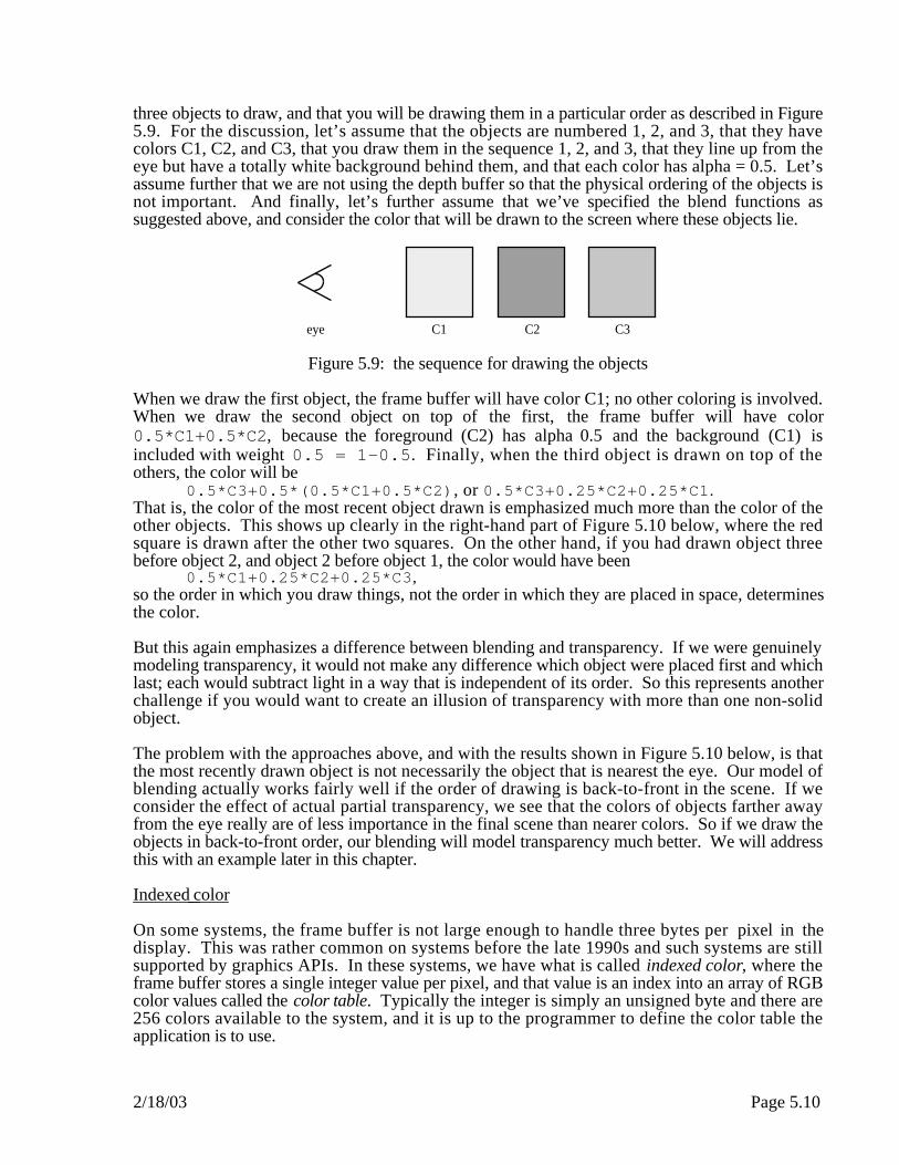
three objects to draw, and that you will be drawing them in a particular order as described in Figure5.9. For the discussion, let’s assume that the objects are numbered 1, 2, and 3, that they havecolors C1, C2, and C3, that you draw them in the sequence 1, 2, and 3, that they line up from theeye but have a totally white background behind them, and that each color has alpha = 0.5. Let’sassume further that we are not using the depth buffer so that the physical ordering of the objects isnot important. And finally, let’s further assume that we’ve specified the blend functions assuggested above, and consider the color that will be drawn to the screen where these objects lie.

C1 C2 C3eye

Figure 5.9: the sequence for drawing the objects

When we draw the first object, the frame buffer will have color C1; no other coloring is involved.When we draw the second object on top of the first, the frame buffer will have color0.5*C1+0.5*C2, because the foreground (C2) has alpha 0.5 and the background (C1) isincluded with weight 0.5 = 1-0.5. Finally, when the third object is drawn on top of theothers, the color will be

0.5*C3+0.5*(0.5*C1+0.5*C2), or 0.5*C3+0.25*C2+0.25*C1.That is, the color of the most recent object drawn is emphasized much more than the color of theother objects. This shows up clearly in the right-hand part of Figure 5.10 below, where the redsquare is drawn after the other two squares. On the other hand, if you had drawn object threebefore object 2, and object 2 before object 1, the color would have been

0.5*C1+0.25*C2+0.25*C3,so the order in which you draw things, not the order in which they are placed in space, determinesthe color.

But this again emphasizes a difference between blending and transparency. If we were genuinelymodeling transparency, it would not make any difference which object were placed first and whichlast; each would subtract light in a way that is independent of its order. So this represents anotherchallenge if you would want to create an illusion of transparency with more than one non-solidobject.

The problem with the approaches above, and with the results shown in Figure 5.10 below, is thatthe most recently drawn object is not necessarily the object that is nearest the eye. Our model ofblending actually works fairly well if the order of drawing is back-to-front in the scene. If weconsider the effect of actual partial transparency, we see that the colors of objects farther awayfrom the eye really are of less importance in the final scene than nearer colors. So if we draw theobjects in back-to-front order, our blending will model transparency much better. We will addressthis with an example later in this chapter.

Indexed color

On some systems, the frame buffer is not large enough to handle three bytes per pixel in thedisplay. This was rather common on systems before the late 1990s and such systems are stillsupported by graphics APIs. In these systems, we have what is called indexed color, where theframe buffer stores a single integer value per pixel, and that value is an index into an array of RGBcolor values called the color table. Typically the integer is simply an unsigned byte and there are256 colors available to the system, and it is up to the programmer to define the color table theapplication is to use.

2/18/03 Page 5.11

Indexed color creates some difficulties with scenes where there is shading or other uses of a largenumber of colors. These often require that the scene be generated as RGB values and the colors inthe RGB scene are analyzed to find the set of 256 that are most important or are closest to thecolors in the full scene. The color table is then built from that analysis.

Besides the extra computational difficulties caused by having to use color table entries instead ofactual RGB values in a scene, systems with indexed color are very vulnerable to color aliasingproblems. Mach banding is one such color aliasing problem, as are color approximations whenpseudocolor is used in scientific applications.

Using color to create 3D images

Besides the stereo viewing technique with two views from different points, there are othertechniques for doing 3D viewing that do not require an artificial eye convergence. When wediscuss texture maps in a later chapter, we will describe a 1D texture map technique that colors 3Dimages more red in the nearer parts and more blue in the more distant parts. An example of this isshown in Figure 1.10. This makes the images self-converge when you view them through a pairof ChromaDepth™ glasses, as we will describe there, so more people can see the spatial propertiesof the image, and it can be seen from anywhere in a room. There are also more specializedtechniques such as creating alternating-eye views of the image on a screen with an overscreen thatcan be given alternating polarization and viewing them through polarized glasses that allow eacheye to see only one screen at a time, or using dual-screen technologies such as head-mounteddisplays. The extension of the techniques above to these more specialized technologies isstraightforward and is left to your instructor if such technologies are available.

Figure 5.10: a ChromaDepth™ display, courtesy of Michael J. Bailey, SDSC

There is another interesting technique for creating full-color images that your user can view in 3D.It involves the red/blue glasses that are familiar to some of us from the days of 3D movies in the1950s and that you may sometimes see for 3D comic books or the like. However, most of thosewere grayscale images, and the technique we will present here works for full-color images.

The images we will describe are called anaglyphs. For these we will generate images for both theleft and right eyes, and will combine the two images by using the red information from the left-eyeimage and the blue and green information from the right-eye image as shown in Figure 5.11. Theresulting image will look similar to that shown in Figure 5.12, but when viewed through red/blue

2/18/03 Page 5.12

(or red/green) glasses with the red filter over the left eye, you will see both the 3D content and thecolors from the original image. This is a straightforward effect and is relatively simple to generate;we describe how to do that in OpenGL at the end of this chapter.

Figure 5.11: creating a blended image from two images

Figure 5.11: an example of a color anaglyphwhen viewed with red/blue or red/green glasses, a 3D color image is seen

This description is from the sitehttp://axon.physik.uni-bremen.de/research/stereo/color_anaglyph/

and the images are copyright by Rolf Henkel. Permission will be sought to use them, or they willbe replaced by new work.

Some examples

Example: An object with partially transparent faces

If you were to draw a piece of the standard coordinate planes and to use colors with alpha less than1.0 for the planes, you would be able to see through each coordinate plane to the other planes asthough the planes were made of some partially-transparent plastic. We have modeled a set of threesquares, each lying in a coordinate plane and centered at the origin, and each defined as having arather low alpha value of 0.5 so that the other squares are supposed to show through. In thissection we consider the effects of a few different drawing options on this view.

2/18/03 Page 5.13

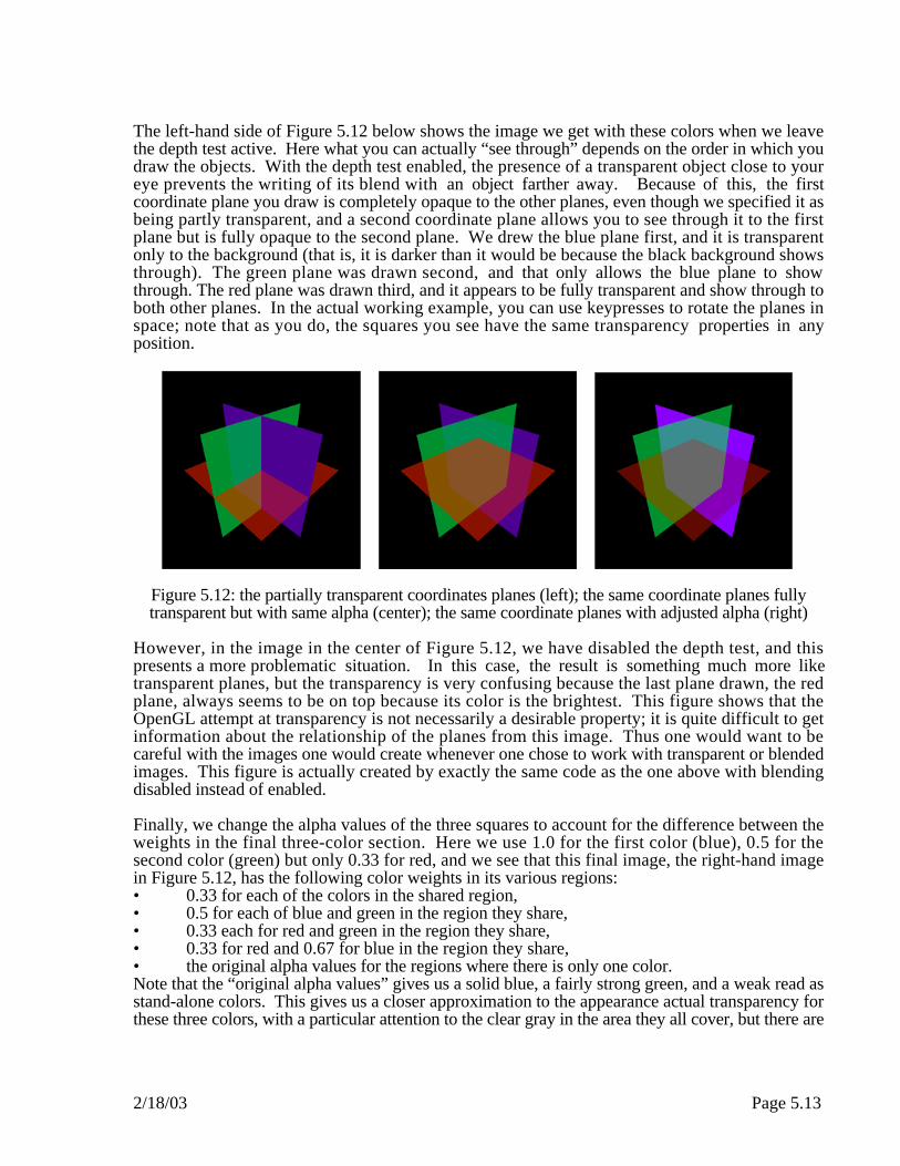
The left-hand side of Figure 5.12 below shows the image we get with these colors when we leavethe depth test active. Here what you can actually “see through” depends on the order in which youdraw the objects. With the depth test enabled, the presence of a transparent object close to youreye prevents the writing of its blend with an object farther away. Because of this, the firstcoordinate plane you draw is completely opaque to the other planes, even though we specified it asbeing partly transparent, and a second coordinate plane allows you to see through it to the firstplane but is fully opaque to the second plane. We drew the blue plane first, and it is transparentonly to the background (that is, it is darker than it would be because the black background showsthrough). The green plane was drawn second, and that only allows the blue plane to showthrough. The red plane was drawn third, and it appears to be fully transparent and show through toboth other planes. In the actual working example, you can use keypresses to rotate the planes inspace; note that as you do, the squares you see have the same transparency properties in anyposition.

Figure 5.12: the partially transparent coordinates planes (left); the same coordinate planes fullytransparent but with same alpha (center); the same coordinate planes with adjusted alpha (right)

However, in the image in the center of Figure 5.12, we have disabled the depth test, and thispresents a more problematic situation. In this case, the result is something much more liketransparent planes, but the transparency is very confusing because the last plane drawn, the redplane, always seems to be on top because its color is the brightest. This figure shows that theOpenGL attempt at transparency is not necessarily a desirable property; it is quite difficult to getinformation about the relationship of the planes from this image. Thus one would want to becareful with the images one would create whenever one chose to work with transparent or blendedimages. This figure is actually created by exactly the same code as the one above with blendingdisabled instead of enabled.

Finally, we change the alpha values of the three squares to account for the difference between theweights in the final three-color section. Here we use 1.0 for the first color (blue), 0.5 for thesecond color (green) but only 0.33 for red, and we see that this final image, the right-hand imagein Figure 5.12, has the following color weights in its various regions:• 0.33 for each of the colors in the shared region,• 0.5 for each of blue and green in the region they share,• 0.33 each for red and green in the region they share,• 0.33 for red and 0.67 for blue in the region they share,• the original alpha values for the regions where there is only one color.Note that the “original alpha values” gives us a solid blue, a fairly strong green, and a weak read asstand-alone colors. This gives us a closer approximation to the appearance actual transparency forthese three colors, with a particular attention to the clear gray in the area they all cover, but there are

2/18/03 Page 5.14

still some areas that don’t quite work. To get even this close, however, we must analyze therendering carefully and we still cannot quite get a perfect appearance.

Let’s look at this example again from the point of view of depth-sorting the things we will draw.In this case, the three planes intersect each other and must be subdivided into four pieces each sothat there is no overlap. Because there is no overlap of the parts, we can sort them so that thepieces farther from the eye will be drawn first. This allows us to draw in back-to-front order,where the blending provides a better model of how transparency operates. Figure 5.13 showshow this would work. The technique of adjusting your model is not always as easy as this,because it can be difficult to subdivide parts of a figure, but this shows its effectiveness.

There is another issue with depth-first drawing, however. If you are creating a scene that permitsthe user either to rotate the eye point around your model or to rotate parts of your model, then themodel will not always have the same parts closest to the eye. In this case, you will need to use afeature of your graphics API to identify the distance of each part from the eyepoint. This is usuallydone by rendering a point in each part in the background and getting its Z-value with the currenteye point. This is a more advanced operation than we are now ready to discuss, so we refer you tothe manuals for your API to see if it is supported and, if so, how it works.

Figure 5.13: the partially transparent planes broken into quadrants and drawn back-to-front

As you examine this figure, note that although each of the three planes has the same alpha value of0.5, the difference in luminance between the green and blue colors is apparent in the way the planewith the green in front looks different from the plane with the blue (or the red, for that matter) infront. This goes back to the difference in luminance between colors that we discussed earlier in thechapter.

Color in OpenGL

OpenGL uses the RGB and RGBA color models with real-valued components. These colorsfollow the RGB discussion above very closely, so there is little need for any special comments oncolor itself in OpenGL. Instead, we will discuss blending in OpenGL and then will give someexamples of code that uses color for its effects.

Specifying colors

In OpenGL, colors are specified with the glColor*(...) functions. These follow the usualOpenGL pattern of including information on the parameters they will take, including a dimension,the type of data, and whether the data is scalar or vector. Specifically we will see functions such as

glColor3f(r, g, b) — 3 real scalar color parameters, orglColor4fv(r, g, b, a) — 4 real color parameters in a vector.

2/18/03 Page 5.15

These allow us to specify either RGB or RGBA color with either scalar or vector data, as we wish.You will see several examples of this kind of color specification throughout this chapter and thelater chapters on visual communication and on science applications.

Enabling blending

In order to use colors from the RGBA model, you must specify that you want the blending enabledand you must identify the way the color of the object you are drawing will be blended with thecolor that has already been defined. This is done with two simple function calls:

glEnable(GL_BLEND);glBlendFunc(GL_SRC_ALPHA, GL_ONE_MINUS_SRC_ALPHA);

The first is a case of the general enabling concept for OpenGL; the system has many possiblecapabilities and you can select those you want by enabling them. This allows your program to bemore efficient by keeping it from having to carry out all the possible operations in the renderingpipeline. The second allows you to specify how you want the color of the object you are drawingto be blended with the color that has already been specified for each pixel. If you use this blendingfunction and your object has an alpha value of 0.7, for example, then the color of a pixel after ithas been drawn for your object would be 70% the color of the new object and 30% the color ofwhatever had been drawn up to that point.

There are many options for the OpenGL blending function. The one above is the most commonlyused and simply computes a weighted average of the foreground and background colors, where theweight is the alpha value of the foreground color. In general, the format for the blendingspecification is

glBlendFunc(src, dest)and there are many symbolic options for the source (src) and destination (dest) blending values;the OpenGL manual covers them all.

A word to the wise...

You must always keep in mind that the alpha value represents a blending proportion, nottransparency. This blending is applied by comparing the color of an object with the current colorof the image at a pixel, and coloring the pixel by blending the current color and the new coloraccording to one of several rules that you can choose with glBlendFunc(...) as noted above.This capability allows you to build up an image by blending the colors of parts in the order inwhich they are rendered, and we saw that the results can be quite different if objects are received ina different order. Blending does not treat parts as being transparent, and so there are some imageswhere OpenGL simply does not blend colors in the way you expect from the concept.

If you really do want to try to achieve the illusion of full transparency, you are going to have to dosome extra work. You will need to be sure that you draw the items in your image starting with theitem at the very back and proceeding to the frontmost item. This process was described in thesecond example above and is sometimes called Z-sorting. It can be very tricky because objects canoverlap or the sequence of objects in space can change as you apply various transformations to thescene. You may have to re-structure your modeling in order to make Z-sorting work. In theexample above, the squares actually intersect each other and could only be sorted if each werebroken down into four separate sub-squares. And even if you can get the objects sorted once, theorder would change if you rotated the overall image in 3-space, so you would possibly have to re-sort the objects after each rotation. In other words, this would be difficult.

As always, when you use color you must consider carefully the information it is to convey. Coloris critical to convey the relation between a synthetic image and the real thing the image is to portray,of course, but it can be used in many more ways. One of the most important is to convey the valueof some property associated with the image itself. As an example, the image can be of some kind

2/18/03 Page 5.16

of space (such as interstellar space) and the color can be the value of something that occupies thatspace or happens in that space (such as jets of gas emitted from astronomical objects where thevalue is the speed or temperature of that gas). Or the image can be a surface such as an airfoil (anairplane wing) and the color can be the air pressure at each point on that airfoil. Color can even beused for displays in a way that carries no meaning in itself but is used to support the presentation,as in the Chromadepth™ display we will discuss below in the texture mapping module. But neveruse color without understanding the way it will further the message you intend in your image.

Code examples

A model with parts having a full spectrum of colors

The code that draws the edges of the RGB cube uses translation techniques to create a number ofsmall cubes that make up the edges. In this code, we use only a simple cube we defined ourselves(not that it was too difficult!) to draw each cube, setting its color by its location in the space:

typedef GLfloat color [4];color cubecolor;

cubecolor[0] = r; cubecolor[1] = g; cubecolor[2] = b;cubecolor[3] = 1.0;glColor4fv(cubecolor);

We only use the cube we defined, which is a cube whose sides all have length two and which iscentered on the origin. However, we don’t change the geometry of the cube before we draw it.Our technique is to use transformations to define the size and location of each of the cubes, withscaling to define the size of the cube and translation to define the position of the cube, as follows:

glPushMatrix();glScalef(scale,scale,scale);glTranslatef(-SIZE+(float)i*2.0*scale*SIZE,SIZE,SIZE);cube((float)i/(float)NUMSTEPS,1.0,1.0);glPopMatrix();

Note that we include the transformation stack technique of pushing the current modelingtransformation onto the current transformation stack, applying the translation and scalingtransformations to the transformation in use, drawing the cube, and then popping the currenttransformation stack to restore the previous modeling transformation. This was discussed earlier inthe chapter on modeling.

The HSV cone

There are two functions of interest here. The first is the conversion from HSV colors to RGBcolors; this is taken from [FvD] as indicated, and is based upon a geometric relationship betweenthe cone and the cube, which is much clearer if you look at the cube along a diagonal between twoopposite vertices. The second function does the actual drawing of the cone with colors generallydefined in HSV and converted to RGB for display, and with color smoothing handling most of theproblem of shading the cone. For each vertex, the color of the vertex is specified before the vertexcoordinates, allowing smooth shading to give the effect in Figure 5.3. For more on smoothshading, see the later chapter on the topic.

voidconvertHSV2RGB(float h,float s,float v,float *r,float *g,float *b){// conversion from Foley et.al., fig. 13.34, p. 593

float f, p, q, t;int k;

if (s == 0.0) { // achromatic case

2/18/03 Page 5.17

*r = *g = *b = v;}else { // chromatic case

if (h == 360.0) h=0.0;h = h/60.0;k = (int)h;f = h - (float)k;p = v * (1.0 - s);q = v * (1.0 - (s * f));t = v * (1.0 - (s * (1.0 - f)));switch (k) {

case 0: *r = v; *g = t; *b = p; break;case 1: *r = q; *g = v; *b = p; break;case 2: *r = p; *g = v; *b = t; break;case 3: *r = p; *g = q; *b = v; break;case 4: *r = t; *g = p; *b = v; break;case 5: *r = v; *g = p; *b = q; break;

}}

}

void HSV(void){#define NSTEPS 36#define steps (float)NSTEPS#define TWOPI 6.28318

int i;float r, g, b;

glBegin(GL_TRIANGLE_FAN); // cone of the HSV spaceglColor3f(0.0, 0.0, 0.0);glVertex3f(0.0, 0.0, -2.0);for (i=0; i<=NSTEPS; i++) {

convert(360.0*(float)i/steps, 1.0, 1.0, &r, &g, &b);glColor3f(r, g, b);glVertex3f(2.0*cos(TWOPI*(float)i/steps),

2.0*sin(TWOPI*(float)i/steps),2.0);}

glEnd();glBegin(GL_TRIANGLE_FAN); // top plane of the HSV space

glColor3f(1.0, 1.0, 1.0);glVertex3f(0.0, 0.0, 2.0);for (i=0; i<=NSTEPS; i++) {

convert(360.0*(float)i/steps, 1.0, 1.0, &r, &g, &b);glColor3f(r, g, b);glVertex3f(2.0*cos(TWOPI*(float)i/steps),

2.0*sin(TWOPI*(float)i/steps),2.0);}

glEnd();}

The HLS double cone

The conversion itself takes two functions, while the function to display the double cone is so closeto that for the HSV model that we do not include it here. The source of the conversion functions isagain Foley et al. This code was used to produce the images in Figure 5.4.

2/18/03 Page 5.18

voidconvertHLS2RGB(float h,float l,float s,float *r,float *g,float *b){// conversion from Foley et.al., Figure 13.37, page 596

float m1, m2;

if (l <= 0.5) m2 = l*(1.0+s);else m2 = l + s - l*s;m1 = 2.0*l - m2;if (s == 0.0) { // achromatic cast

*r = *g = *b = l;}else { // chromatic case

*r = value(m1, m2, h+120.0);*g = value(m1, m2, h);*b = value(m1, m2, h-120.0);

}}

float value( float n1, float n2, float hue) {// helper function for the HLS->RGB conversion

if (hue > 360.0) hue -= 360.0;if (hue < 0.0) hue += 360.0;if (hue < 60.0) return( n1 + (n2 - n1)*hue/60.0 );if (hue < 180.0) return( n2 );if (hue < 240.0) return( n1 + (n2 - n1)*(240.0 - hue)/60.0 );return( n1 );

}

An object with partially transparent faces

The code that draws three squares in space, each centered at the origin and lying within one of thecoordinate planes, has a few points that are worth noting. These three squares are coloredaccording to the declaration:

GLfloat color0[]={1.0, 0.0, 0.0, 0.5}, // R color1[]={0.0, 1.0, 0.0, 0.5}, // G color2[]={0.0, 0.0, 1.0, 0.5}; // B

These colors are the full red, green, and blue colors with a 0.5 alpha value, so when each square isdrawn it uses 50% of the background color and 50% of the square color. You will see thatblending in Figure 5.10 for this example.

The geometry for each of the planes is defined as an array of points, each of which is, in turn, anarray of real numbers:

typedef GLfloat point3[3];point3 plane0[4]={{-1.0, 0.0, -1.0}, // X-Z plane

{-1.0, 0.0, 1.0}, { 1.0, 0.0, 1.0}, { 1.0, 0.0, -1.0} };

As we saw in the example above, the color of each part is specified just as the part is drawn:glColor4fv(color0); // redglBegin(GL_QUADS); // X-Z plane

glVertex3fv(plane0[0]);glVertex3fv(plane0[1]);glVertex3fv(plane0[2]);glVertex3fv(plane0[3]);

2/18/03 Page 5.19

glEnd();This is not necessary if many of the parts had the same color; once a color is specified, it is usedfor anything that is drawn until the color is changed.

To extend this example to the example of Figure 5.11 with the back-to-front drawing, you need tobreak each of the three squares into four pieces so that there is no intersection between any of thebasic parts of the model. You then have to arrange the drawing of these 12 parts in a sequence sothat the parts farther from the eye are drawn first. For a static view this is simple, but as wepointed out in the chapter above on modeling, to do this for a dynamic image with the parts or theeyepoint moving, you will need to do some depth calculations on the fly. In OpenGL, this can bedone with the function GLint gluProject(objX,objY,objZ,model,proj,view,winX,winY,winZ)where objX, objY, and objZ are the GLdouble coordinates of the point in model space,model and proj are const GLdouble * variables for the current modelview and projectionmatrices (obtained from glGetDoublev calls), view is a const Glint * variable for thecurrent viewport (obtained from a glGetIntegerv call), and winX, winY, and winZ areGLdouble * variables that return the coordinates of the point after projection into 3D eye space.

With this information, you can determine the depth of each of the components of your scene andthen associate some kind of sequence information based on the depth. This allows you to arrangeto draw them in back-to-front order if you have structured your code, using techniques such asarrays of structs that include quads and depths, so you can draw your components by operating onthe quads in depth order.

Indexed color

In addition to the RGB and RGBA color we have discussed in this chapter, OpenGL can operate inindexed color mode. However, we will not discuss this here because it introduces few newgraphics ideas and is difficult to use to achieve high-quality results. If you have a system that onlysupports indexed color, please refer to the OpenGL reference material for this information.

Creating anaglyphs in OpenGL

The techniques for creating anaglyphs use more advanced features of OpenGL’s color operations.As we saw in Figure 5.10, we need to have both the left-eye and right-eye versions of the image,and we will assume that the images are full RGB color images. We need to extract the red channelof the left-eye image and the green and blue channels of the right-eye image. We will do this bygenerating both images and saving them to color arrays, and then assembling the parts of the twoimages into one image by using the red information from the left-eye image and the blue and greeninformation from the right-eye image.

To get these two color arrays for our computer-generated image, you will generate the left-eyeimage into the back buffer and save that buffer into an array so we can use it later. If you arecreating a synthetic image, create the image as usual but do not call glutSwapBuffers(); ifyou are using a scanned image, read the image into an array as specified below. The back buffer isspecified as the buffer for reading with the glReadBuffer(GL_BACK) function. You can thenread the contents of the buffer into an array left_view with the function

glReadPixels(0,0,width,height,GL_RGB,GL_UNSIGNED_BYTE,left_view)where we assume you are reading the entire window (the lower left corner is (0,0) ), your windowis width pixels wide and height pixels high, you are drawing in RGB mode, and your data isto be stored in an array left_view that contains 3*width*height unsigned bytes (of typeGLUByte). The array needs to be passed by being cast as a (GLvoid *) parameter. You coulduse another format for the pixel data, but the GL_UNSIGNED_BYTE seems simplest here.

2/18/03 Page 5.20

After you have stored the left-eye image, you will do the same with the right-eye image, storing itin an array right_view, so you have two arrays of RGB values in memory. Create a third arraymerge_view of the same type, and loop through the pixels, copying the red value from theleft-view pixel array and the green and blue values from the right-view pixel array. Younow have an array that merges the colors as in Figure 5.10. You can write that array to the backbuffer with the function

glDrawPixels(width,height,GL_RGB,GL_UNSIGNED_BYTE,merge_view)with the parameters as above. This will write the merge_view array back into the frame buffer,and it will be displayed by swapping the buffers.

Note that the image of Figure 5.11 is built from grayscale left and right views. This means that allthe parts of the image will have red, green, and blue color information, so all of them will bedistinguishable in the merged anaglyph. If the image has a region where the red channel or both ofthe green and blue channels are zero (which can happen with a synthetic image, more likely thanwith a scanned real-world image), the anaglyph could have no information in that region for botheyes and could fail to work well.

Summary

In this chapter we have presented a general discussion of color that includes the RGB, RGBA,HLS, and HSV color models. We included information on color luminance and techniques forsimulating transparency with the blending function of the alpha channel, and we introduced a wayto generate 3D images using color. Finally, we showed how color is specified and implemented inOpenGL. You should now be able to use color easily in your images, creating much moreinteresting and meaningful results than you can get with geometry alone.

Questions

1. Look at a digital photograph or scanned image of the real world, and compare it with agrayscale version of itself (for example, you can print the image on a monochrome printer orchange your computer monitor to show only grayscale). What parts stand out more in thecolor image? In the monochrome image?

2. Look at a standard color print with good magnification (a large magnifying glass, a loupe, etc.)and examine the individual dots of each CMYK color. Is there a pattern defined for theindividual dots of each color? How do varying amounts of each color make the actual coloryou see in the image?

3. Look at the controls on your computer monitor, and find ways to displays colors of differentdepth. (The usual options are 256 colors, 4096 colors, or 16.7 million colors.) Display animage on the screen and change between these color depth options, and observe thedifferences; draw some conclusions. Pay particular attention to whether you see Mach bands.

Exercises

4. Identify several different colors with the same luminance and create a set of squares next toeach other on the screen that are displayed with these colors. Now go to a monochromeenvironment and see whether the colors of the squares are differentiable.

5. Create a model of the RGB color cube in OpenGL, with the faces modeled as quads andcolored by blending the colors at the vertices. View this RGB cube from several points to seehow the various faces look. Modify the full RGB cube by scaling the vertices so that the

2/18/03 Page 5.21

largest color value at each of the vertices is C, where C lies between 0 and 1, for a value of Cyou determine however you like.

6. Many computers or computer applications have a “color picker” capability that allows you tochoose a color by RGB, HSV, or HLS specifications. Choose one or two specific colors andfind the RGB, HSV, and HLS color coordinates for each, and then hand-execute the colorconversion functions in this chapter to verify that each of the HSV and HLS colors converts tothe correct RGB.

7. You can use the color picker from the previous exercise to find the RGB values for a givencolor by comparing the given color (which might, in fact, be the color of a physical object)with the color that is presented by the color picker. Make an initial estimate of the color, andthen change the RGB components bit by bit to get as good a match as you can.

8. Create two planes that are very close and that cross at a very shallow angle, and color them inquite different colors. See if you get z-fighting at the intersection of these two planes. Nowtake exactly the same planes, offset by a very small amount, and see what kind of z-fightingyou observe. How does the color help you see what the geometry is doing?

9. (Class project) There is a technique called the Delphi method for estimating an answer to anumeric question. In this technique, a number of people each give their answers, and theanswers are averaged to create an overall estimate. Do this with RGB values for the colors ofobjects: have everyone in the class estimate the RGB colors of an object and average theindividual estimates, and see how close the combined estimate is to the RGB color as youwould determine it by the previous exercise.

10.(Painter’s algorithm) Take any of your images that is defined with a modest number ofpolygons, and instead of using depth buffering to accomplish hidden surfaces, use thePainter’s Algorithm: draw the polygons from the farthest to the nearest. Do this by creating anarray or list of all the polygons you will use and get their distances from the eye with theOpenGL gluProject(...) function as described in this chapter, and then sort the array orlist and draw the polygons in distance order.

Experiments

11.(Blending) Draw two or three planar objects on top of each other, with different alpha values inthe color of the different objects. Verify the discussion about what alpha values are needed tosimulate equal colors from the objects in the final image, and try changing the order of thedifferent objects to see how the alpha values must change to restore the equal color simulation.

12.(Anaglyph) If your instructor can get red/cyan glasses, identify a stereo pair of images that youcan work with. This can be a pair of computed images or a pair of digital photographs. Agood choice could be a slide from a stereopticon (and old-fashioned stereo viewer), with twograyscale images with views from two viewpoints. Create an anaglyph for the image and viewit through the glasses to see both the color and depth information the anaglyph contains.

Projects

13.(The small house) For the small house project you have seen in several earlier chapters,modify the colors of the walls to include an alpha value and arrange the modeling so that youcan see the structure of the house from outside by using blending.

2/18/03 Page 5.22

14.(A scene graph parser) Modify the scene graph parser you began in an earlier chapter to allowyou to specify the color of an object in the appearance node of a geometry node for the object,and write the code for that appearance before the geometry code is written. For efficiency, youshould check whether the color has changed before writing a code statement to change thecolor, because color is generally retained by the system until it is specifically changed.