chapter 5 discrete probability distributions. probability experiment a probability experiment is any...
TRANSCRIPT
Chapter 5
Discrete Probability Distributions
Probability Experiment
A probability experiment is any activity that produces uncertain or “random” outcomes
Random Variable
A random variable is a rule or function that translates the outcomes of a probability experiment into numbers.
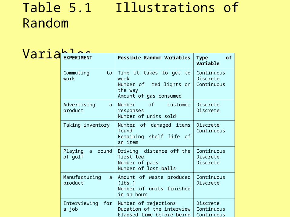
Table 5.1 Illustrations of Random Variables
EXPERIMENT Possible Random Variables Type of Variable
Commuting to work Time it takes to get to workNumber of red lights on the wayAmount of gas consumed
ContinuousDiscreteContinuous
Advertising a product Number of customer responsesNumber of units sold
DiscreteDiscrete
Taking inventory Number of damaged items foundRemaining shelf life of an item
DiscreteContinuous
Playing a round of golf Driving distance off the first teeNumber of parsNumber of lost balls
ContinuousDiscreteDiscrete
Manufacturing a product Amount of waste produced (lbs.)Number of units finished in an hour
ContinuousDiscrete
Interviewing for a job Number of rejectionsDuration of the interviewElapsed time before being hired
DiscreteContinuousContinuous
Buying stocks Number of your stocks that increase in valueAmount of sleep lost from worry
DiscreteContinuous
Discrete Random Variable
A discrete random variable has separate and distinct values, with no values possible in between.

Continuous Random Variable
A continuous random variable can take on any value over a given range or interval.
Probability Distribution
A probability distribution identifies the probabilities that are assigned to all possible values of a random variable.
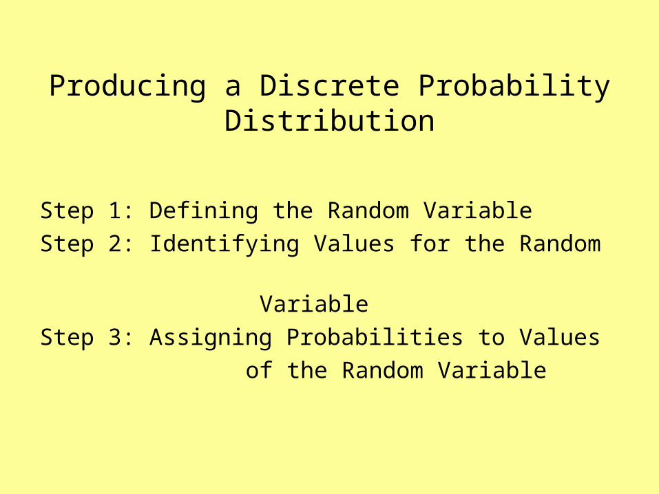
Producing a Discrete Probability Distribution
Step 1: Defining the Random Variable
Step 2: Identifying Values for the Random
Variable
Step 3: Assigning Probabilities to Values
of the Random Variable
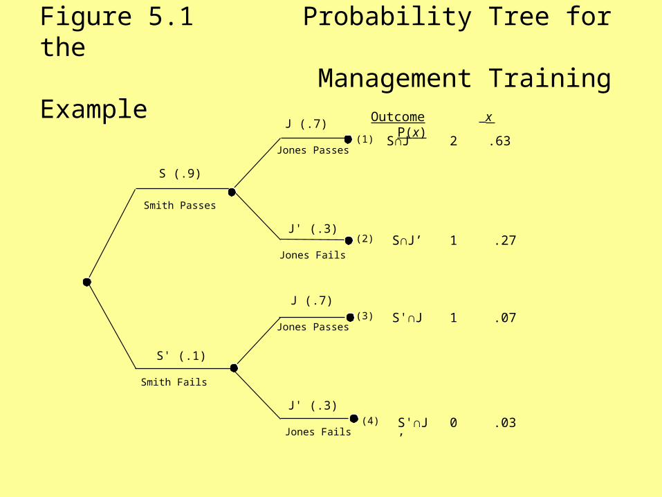
Figure 5.1 Probability Tree for the Management Training Example
J (.7)
Jones Fails
S (.9)
J (.7)
S' (.1)
Smith Passes
Smith Fails
Jones Passes
S∩J
S∩J’
S'∩J
S'∩J’
2
1
1
0
.63
.27
.07
.03
Jones Fails
J' (.3)
Jones Passes
J' (.3)
(1)
(2)
(3)
(4)
Outcome x P(x)
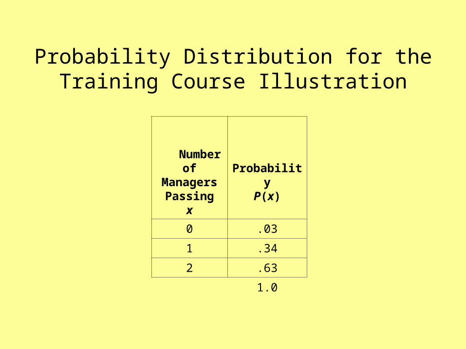
Probability Distribution for the Training Course Illustration
Number ofManagers Passing
xProbability
P(x)
0 .03
1 .34
2 .63
1.0
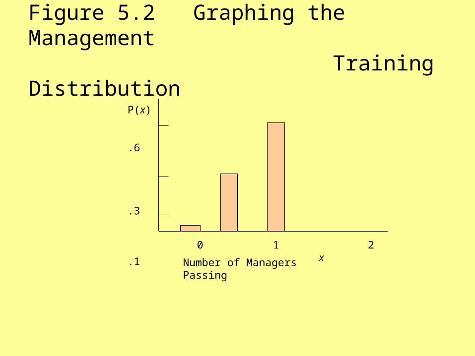
Figure 5.2 Graphing the Management Training Distribution
P(x)
.6
.3
.1
Number of Managers Passing
0 1 2 x
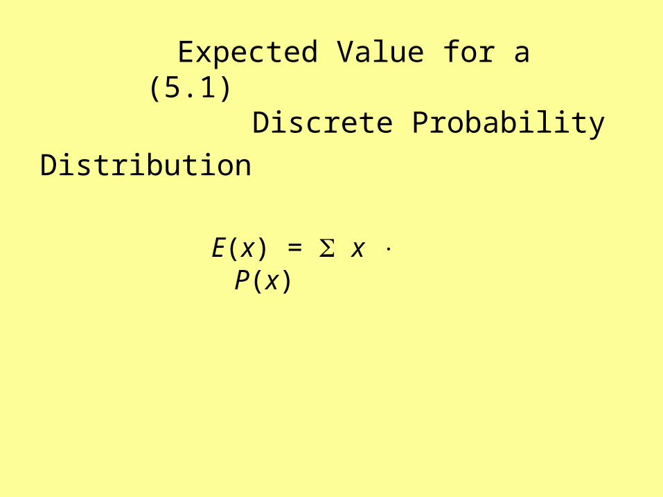
Expected Value for a (5.1)
Discrete Probability Distribution
E(x) = x P(x)
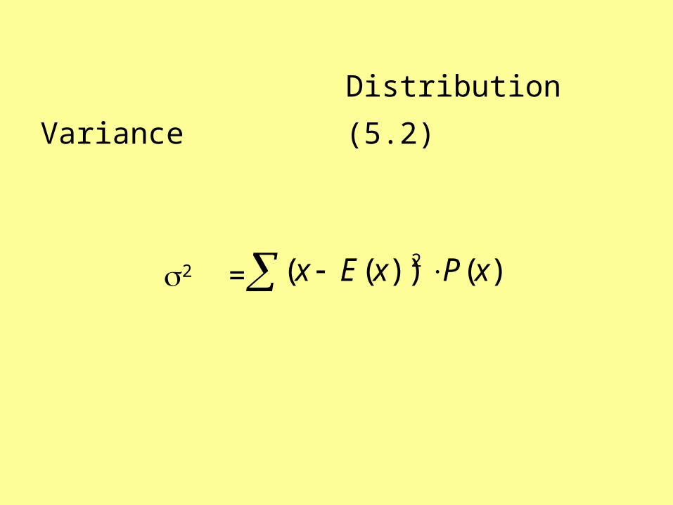
Distribution Variance (5.2)
2 = )())(( 2 xPxEx
The Binomial Distribution
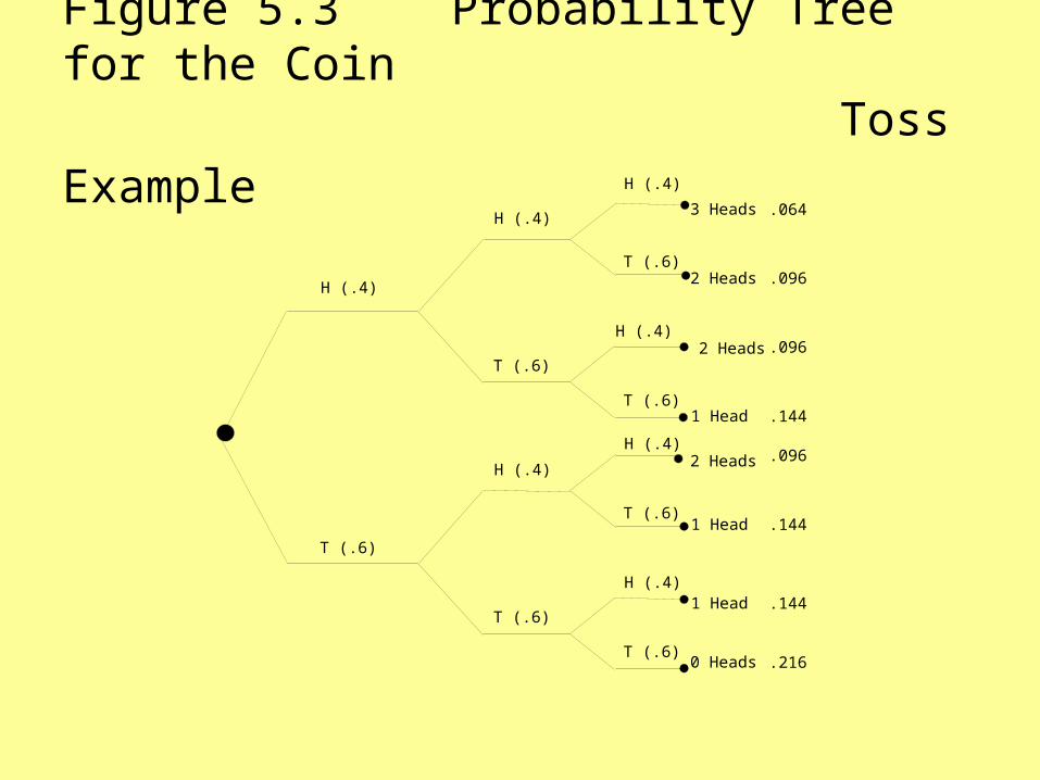
Figure 5.3 Probability Tree for the Coin
Toss Example
H (.4)
H (.4)
H (.4)
T (.6)
T (.6)
H (.4)
.096
T (.6)
H (.4).096
H (.4)
T (.6)
H (.4)
T (.6)
T (.6)
T (.6)
.144
.144
.144
.216
.0643 Heads
.096
2 Heads
2 Heads
1 Head
2 Heads
1 Head
1 Head
0 Heads
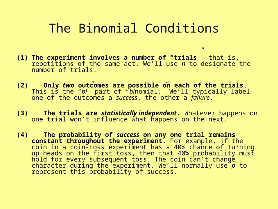
The Binomial Conditions
(1) The experiment involves a number of “trials”— that is, repetitions of the same act. We’ll use n to designate the number of trials.
(2) Only two outcomes are possible on each of the trials. This is the “bi” part of “binomial.” We’ll typically label one of the outcomes a success, the other a failure.
(3) The trials are statistically independent. Whatever happens on one trial won’t influence what happens on the next.
(4) The probability of success on any one trial remains constant
throughout the experiment. For example, if the coin in a coin-toss experiment has a 40% chance of turning up heads on the first toss, then that 40% probability must hold for every subsequent toss. The coin can’t change character during the experiment. We’ll normally use p to represent this probability of success.
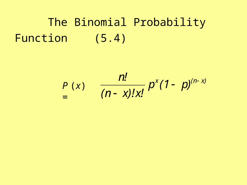
The Binomial Probability Function (5.4)
n!
(n x)!x!p (1 p)x (n x)
P (x) =
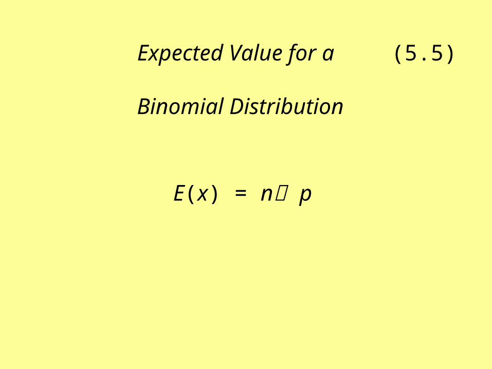
Expected Value for a (5.5) Binomial Distribution
E(x) = n ּ p
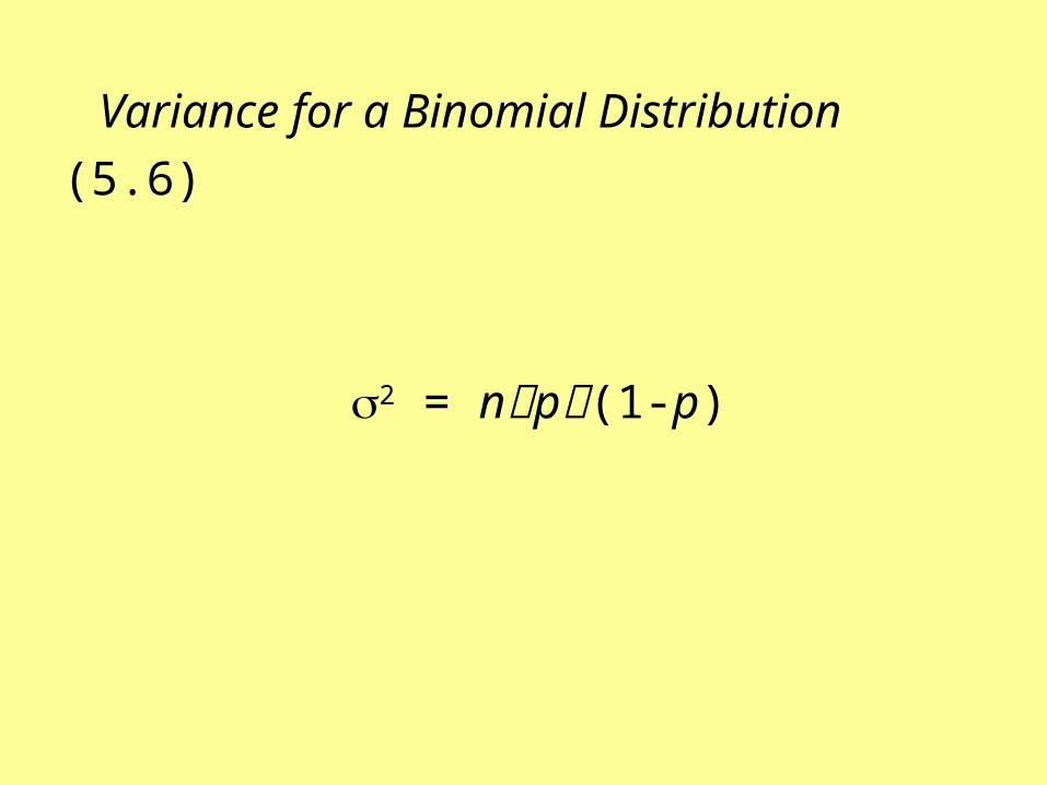
Variance for a Binomial Distribution (5.6)
2 = n ּp ּ(1-p)

Standard Deviation for a (5.7) Binomial Distribution
= )1( ppn

Symmetric
Figure 5.4 Some Possible Shapes
for a Binomial Distribution
Positively Skewed
0 1 2 3 4 5 6 x
P(x)
0 1 2 3 4 5 6 x
P(x)
Negatively Skewed
0 1 2 3 4 5 6 x
P(x)
The Poisson Distribution
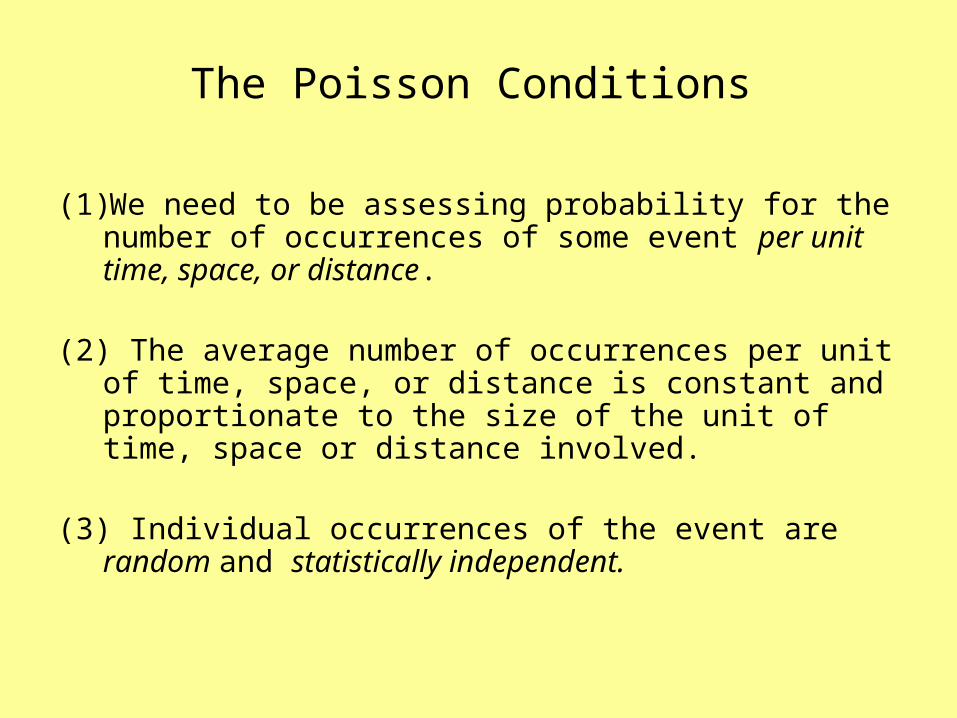
The Poisson Conditions
(1) We need to be assessing probability for the number of
occurrences of some event per unit time, space, or distance.
(2) The average number of occurrences per unit of time, space, or distance is constant and proportionate to the size of the unit of time, space or distance involved.
(3) Individual occurrences of the event are random and statistically independent.
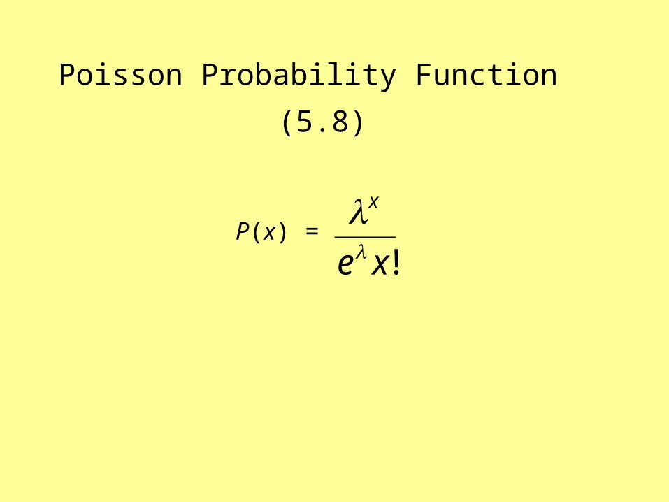
Poisson Probability Function (5.8)
P(x) = !xe
x
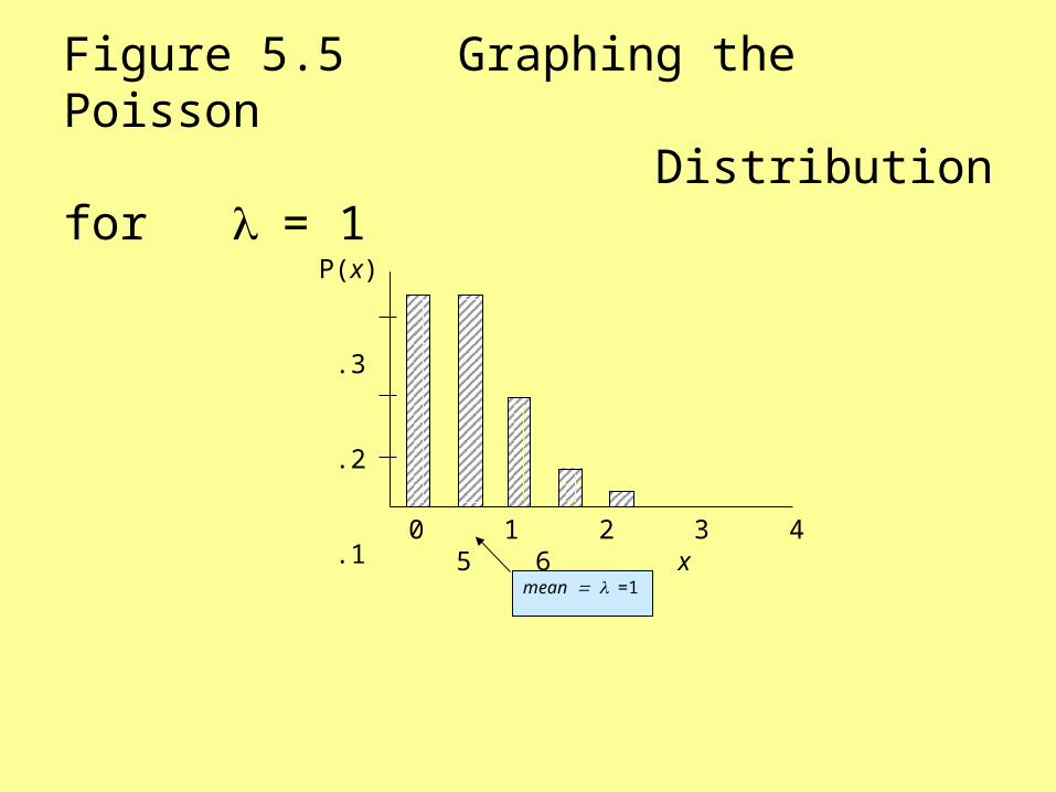
Figure 5.5 Graphing the Poisson Distribution for = 1
mean=1
P(x)
.3
.2
.1
0 1 2 3 4 5 6 x
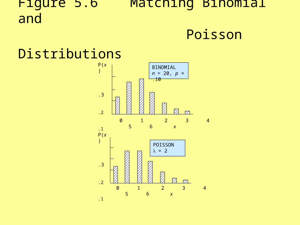
Figure 5.6 Matching Binomial and
Poisson Distributions
0 1 2 3 4 5 6 x
P(x) .3
.2
.1
BINOMIALn= 20, p = .10
POISSON= 2
P(x) .3
.2
.1
0 1 2 3 4 5 6 x