Chapter 5Little's Law

John D.C. Little and Stephen C. GravesMassachusetts Institute of Technology

The average waiting time and the average number of items waiting for..a servicein a service system are important measurements for a manager. Little's Lawrelates these two metrics via the average rate of arrivals to the system. Thisfunda-mental law has found numerous uses in operations management and managerialdecision making.

Introduction

Caroline is a wine buff and bon vivant. She likes to stop at her local wine store,Transcendental Tastings, on the way home from work. She browses the aisles look-ing for the latest releases from her favorite vineyards. Occasionally she picks up afew bottles. She stores these in a rack in a cool corner of her cellar. She and her

partner eat out frequently but when they are at home they usually split a bottle ofwine at dinner. Sometimes they have friends over and that puts a bigger ,dentin thewine inventory.

They have been doing this for some time. Her wine rack holds 240 bottles. Shenotices that she seldom fills the rack to the top but sometimes after a good party therack is empty. On average it seems to be about 2/3rds full, which would equate to160 bottles.

Many wines improve with age. After reading an article about this, Carolinestarts to wonder how long, on average, she has been keeping her wines. She wentback through a few months of wine invoices from Transcendental and estimatesthat she has bought, on average, about eight bottles per month. But she certainlydoesn't know when she drank which bottle and so there seems to be no way shecan find out, even approximately, the average age of the bottles she has beendrinking.

This is a good task for Little's Law.

D. Chhajed and TJ. Lowe (eds.) Building Intuition: Insights From BasicOperations Management Models and Principles.doi: 10.1007/978-0-387 -73699-0, <9Springer Science + Business Media, LLC 2008

81

82 J.D.C. Little, S.c. Graves

Little's Law Deals with Queuing Systems

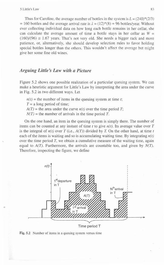
A "queuing system" consists of discrete objects we shall call "items" that "arrive" atsome rate to the "system." Within the system the items may form one or more queuesand eventually receive "service" and exit. Figure 5.1 shows this schematically.

Arrivals -~ queuing system: items in 1- Departuresqueue & items in service

I

Flow of items through a queuing system

Fig. 5.1 Schematic view of a queuing system

While items are in the system, they may be in queues ,or may be in service orsome in queue and some in service. The interpretation will depend on the applica-tion and the goals of the modeler.For example in the case of the wine cellar, we saythat a bottle (an "item") arrives to the system when it is first placed into the winecellar. Each bottle remains in the system until Caroline selects it and removes itfrom the cellar for consumption. If 'we view the wine rack as a single channelserver, the service time is the time between successive removals. It is interesting tonote, however, that we do not know which bottle Caroline will pick and there is noparticular reason to believe that she will pick according to a first-in, first-out (FIFO)rule. In any case, to deal with the average number of bottles in the cellar or averagetime spent by a bottle in the cellar, we need to consider the complete system con-sisting of queue plus service.

Little's Law says that, under steady state conditions, the average number ofitems in a queuing system equals the average rate at which items arrive multipliedby the average time that an item spends in the system. Letting

L =average number of items in the queuing system,W = average waiting time in the system for an item, andA =average number of items arriving per unit time, the law is

L=AW (1)

This relationship is remarkably simple and general. We require stationarityassumptions about the underlying stochastic processes, but it is quite surprisingwhat we do not require. We have not mentioned how many servers there are,whether each server has its own queue or a single queue feeds all servers, what theservice time distributions are, or what the distribution of inter-arrival times is, orwhat is the order of service of items, etc.

In good part because of its simplicity and generality, the equation (1) isextremely useful. It is especially handy for "back of the envelope" calculations.The reason is that two of the terms in (1) may be easy to estimate and not the third.Then Little's Law quickly provides the missing value.

5 Little's Law 83

Thus for Caroline, the average number of bottles in the system is L =(240)*(2/3)

= 160 bottles and the average arrival rate is A =(12)*(8) =96 bottles/year. Withoutever collecting individual data on how long each bottle remains in her cellar, shecan calculate the average amount of time a bottle stays in her cellar as W =(160)/(96) == 1.67 years. That's not very old. She needs a bigger rack and morepatience, or, alternatively, she should develop selection rules to favor holdingspecial bottles longer than the others. This wouldn't affect the average but mightgive her some fine old wines.

Arguing Little's Law with a Picture

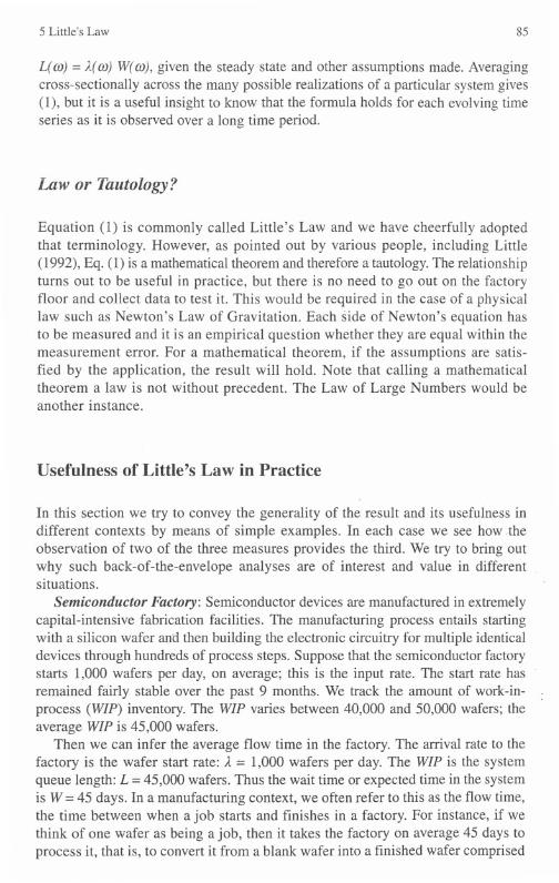
Figure 5.2 shows one possible realization of a particular queuing system. We canmake a heuristic argument for Little's Law by interpreting the area under the curvein Fig. 5.2 in two different ways. Let

n( t) =the number of items in the queuing system at time t;T =a long period of time;A(T) =the area under the curve n( t) over the time period T;N(T) =the number of arrivals in the time period T.

'"

On the one hand, an item in the queuing system is simply there. The number ofitems can be counted at any instant of time t to give n(t). Its average value over Tis the integral of n(t) over T (i.e., A(T)) divided by T. On the other hand, at time teach of the items is waiting and so is accumulating waiting time. By integrating n(t)over the time period T, we obtain a cumulative measure of the waiting time, againequal to A(T). Furthermore, the arrivals are countable too, and given by N(T).Therefore, inspecting the figure, we define

n(t)

1stdepartureinT

Time period T

Fig.5.2 Number of items in a queuing system versus time

84 lD.C. Little, S.c. Graves

A(T) =N(T)/T =arrival rate during time period T,L(T) =A(T)/T =average queue length during time period T,W(T) =A(T)/N(T) =average waiting time in the system per arrival during T.A slight manipulation gives L(T) =A(T)W(T).

All of these quantities wiggle around a little as T increases because of the sto-chastic nature of the queuing process and because of end effects. End effects referto the inclusion in W(T) of some waiting by items which joined the system prior tothe start of T and the exclusion of some waiting by items who arrived during T buthave not left yet. As T increases, L(T) and A(T) go up and down somewhat as itemsarrive and later leave.

Under appropriate mathematical assumptions about the stationarity of theunderlying stochastic processes, the end effects at the start and finish of Tbecome negligible compared to the main area under the curve. Thus, as T

- increases, these stochastic "wiggles" in L(T), A(T), and'W(T) become smallerand smaller percentages of their eventual values so that L(T), A(T), and W(T)each go to a limit as we increase T to infinity. Then, using the obvious symbolsfor the limits, we have:

limL(T)= L;T~oo lim A(T)= A;T~oo lim W (T):T~oo

from which we get the desired result (1).It is interesting and important to note that the formula holds for each realization

of the queuing system over time. This was argued by Little, in his original paper(Little 1961), noting that the relationship (1) held for each evolution of the timeseries of a particular queuing system. In other words, if we watch a specific case orrealization designated, say, by OJ,as it develops over time, then we will find that

5 Little's Law 85

L( m) =A(m) W(my,given the steady state and other assumptions made. Averagingcross-sectionally across the many possible realizations of a particular system gives(1), but it is a useful insight to know that the formula holds for each evolving timeseries as it is observed over a long time period.

Law or Tautology?

Equation (1) is commonly called Little's Law and we have cheerfully adoptedthat terminology. However, as pointed out by various people, including Little(1992), Eq. (1) is a mathematicaltheorem and therefore a tautology.The relationshiptu'rns out to be useful in practice, but there is no need to go out on the factoryfloor and collect data to test it. This would be required in the case of a physicallaw such as Newton's Law of Gravitation. Each side of Newton's equation hasto be measured and it is an empirical question whether they are equal within themeasurement error. For a mathematical theorem, if the assumptions are satis-fied by the application, the result will hold. Note that calling a mathematicaltheorem a law is not without precedent. The Law of Large Numbers would beanother instance.

Usefulness of Little's Law in Practice

In this section we try to convey the generality of the result and its usefulness indifferent contexts by means of simple examples. In each case we see how ,theobservation of two of the three measures provides the third. We try to bring outwhy such back-of-the-envelope analyses are of interest and value in differentsituations.

Semiconductor Factory: Semiconductor devices are manufactured in extremelycapital-intensive fabrication facilities. The manufacturing process entails startingwith a silicon wafer anti then building the electronic circuitry for multiple identicaldevices through hundreds of process steps. Suppose that the semiconductor factorystarts 1,000 wafers per day, on average; this is the input rate. The start rate has'remained fairly stable over the past 9 months. We track the amount of work-in-process (WIP) inventory. The WIP varies between 40,000 and 50,000 wafers; theaverage WIP is 45,000 wafers.

Then we can infer the average flow time in the factory. The arrival rate to thefactory is the wafer start rate: A.= 1,000 wafers per day. The WIP is the systemqueue length: L =45,000 wafers. Thus the wait time or expected time in the systemis W =45 days. In a manufacturing context, we often refer to this as the flow time,the time between when a job starts and finishes in a factory. For instance, if wethink of one wafer as being a job, then it takes the factory on average 45 days toprocess it, that is, to convert it from a blank wafer into a finished wafer comprised

86 J.D.C. Little, S.C. Graves

of electronic devices. Knowing the flow time is critical for planning and schedul-ing the factory, and for making delivery commitments to customers. We shallreturn later to the connection between Little's Law and operations management.

E-Mail: Managing our e-mail is a common and,time-consuming daily activity.For many it is hard to keep up with the volume of messages, let alone providetimely responses. A student Sue might receive 50 messages each day to which shemust generate a response. Can we easily assess how well this student handles here-mail duties?

Indeed we can apply Little's Law to get a quick sense of how promptly Sueresponds to messages. Suppose that she receives about 50 messages every day;then this is the arrival rate: A=50 messages/day. Suppose we can also track howmany messages have yet to be answered. For instance, suppose that Sueremoves a message from her InBox once she has responded to it. Then theremaining messages in her InBox are the messages that are waiting to beanswered. Over the last semester, the size of the InBox has varied between oneand two hundred messages with an average of 150 messages. Then we canregard this to be the system queue length: L = 150 messages. From Little's Lawwe immediately have an estimate of how long it takes Sue to answer a message,on average: W = 3 days.

Hospital Ward: We wish to determine the size and staffing levels for thematernity ward for a local hospital. From historical records we know that thebirth rate for the local community is about five births per day. We also know thatmost women stay in the maternity ward for 2 days before going home with child;however occasionally, there are complications with the birth that require muchlonger stays. Over the past 6 months, we find that 90% of the births haveresulted in 2-day stays; for the remaining 10% of the cases, the average lengthof time in the maternity ward is 7 days. Thus, on average, the length of stay is0.9 x 2 + 0.1 x 7 = 2.5 days.

We can use Little's Law to predict the average number of mothers in the mater-nity ward. The arrival process corresponds to the women arriving to deliver theirbabies; the arrival rate is A =5 mothers per day. The relevant waiting time in thesystem is the length of stay in the maternity ward: W =2.5 days. Thus, the expectedqueue length or number in the system is L =12.5 mothers. This would be useful indetermining the size of the maternity ward (e.g., beds) and the staffing require-ments. However, the law only provides the average requirements, and one wouldneed to design the maternityward to accommodateits peak requirements.For instance,we would certainly want more than 12.5or 13beds in order to handle the variabilityin the occupancy of the ward. One needs to use queuing models and/or simulationto explore the trade-offs between the utilization of the beds and the likelihood ofnot having a bed for an expectant mother. Nevertheless, Little's Law provides astarting point for this investigation, since we know the average number of beds thatare needed.

TollBooths: The TedWilliamsTunnel travelsunder the Boston harbor,connectingEast Boston to South Boston. During the course of a day, about 50,000 vehicles gothrough the tolls at the entry point to the Tunnel in East Boston. The Massachusetts

5 Little's Law 87

Transit Authority (MTA) tries to modulate the number of toll booths that are openat any point in time so that the average number of vehicles waiting at the tolls(including those at the booths) never exceeds 20 vehicles. For instance, all sixbooths are open during the peak time in the morning from 6:00 AM to 10:00 AM.During this morning rush hour, the tunnel handles up to 4,000 cars per hour, andthe MTA estimates that the average number of vehicles waiting at any point of timeis near the target maximum of 20 vehicles.

With the assumption that the alTivalsoccur at a relatively stable rate over themorning rush hour, we can then use Little's Law to ask what quality of service isbeing delivered in terms of average waiting time per vehicle. Suppose that the anivalrate to the toll booths is A.=3,600 vehicles per hour (or I vehicle per second),and theexpected number of vehicles in the system is L =20 vehicles. Thus, on average, thetime a vehicle spends at the toll booths is W = 20/3,600h = 20 s.

Housing Market: The local real estate agent in your community estimatesthat it takes 120 days on average to sell a house; whereas this number changessome with the economy and season, it has been fairly stable over the past decade.You observe from monitoring the classified ads that over the past year thenumber of houses for sale has ranged from 20 to 30 at any point in time, withan average of 25. What can we say about the number of transactions in thepast year?

From Little's Law we can estimate this by viewing the real estate market as aqueuing system. We regard a house being put up for sale as an arrival to the sys-tem. We assume that an unsold house remains on the market until it is sold. Thus,when a house "completes its service" and departs from the market, we infer that ithas been sold. We have estimates of the average time in the system and the averagenumber in the system, namely, W = 120 days and L = 25 houses. From this, we canestimate the arrival rate to the system, A.= 25/120 houses per day ==75 houses

per year.Doughnut Shop: From your daily morning trip to the doughnut shop, you know

they have a healthy business, at least financially speaking. As you might want toinvest in a franchise, you wonder what amount of revenue they generate. Over thecourse of several months; you visit the shop at random times between 6:00 AM and9:00 AM; you observe that the queue averages about 10 customers, and that it takesyou about 3 min to get in and out of the shop.

If you assume your experience is typical, then you can apply Little's Lawto estimate what.the throughput rate is for the enterprise for the morning peakperiod. The expected number in the system is L = 10 customers and theexpected time in the system is W = 3 min. We can then estimate the arrival

rate to the system, namely A.= 10/3 customers per minute =200 customers perhour. We also term this the throughput rate as arriving customers becomethroughput once served. To get an estimate for the revenue potential from thisshop, we need to estimate how much each customer spends. If you typicallyspend $5 per visit, then with the assumption that you are a typical customer,we have a rough estimate of the shop's revenue during these morning hours,i.e., $1,000 per hour.

88 lD.C. Little, S.C. Graves

The Robustness and Generality of Little's Lawin Certain Systems

So far we have developed and discussed Little's Law as a relationship amongsteady-state stochastic processes. The contexts we have examined have been well-behaved, stable, and on-going. In particular we assume that the characteristics ofthe arrival and service processes are stationary over time. For example, in the caseof the maternity ward, we assume that the average arrival rate of mothers has been

: steady at five per day for some time, and that this rate does not vary with day ofweek or season of the year. Similarly, we have regarded the service process as

, beingstationary;for instance,weread andprocessour e-mailat roughlythe sameaverage rate, day in and day out, independent of the backlog of unread messages.For some of our examples, we have focused on an interval of time, e.g., the morn-ing rush hour through the toll booths. However, in these instances due to the hugevolume of arrivals, we contend that the system behavior is virtually equivalent tothat of a steady-state system.

The purpose of this section is to show the great robustness and generality ofLittle's Law under certain circumstances. Indeed Little's Law is exact in thesecases even though arrival and service process may be nonstationary. The essentialcondition is to have a finite window of observation that starts and stops whenthe system is empty. We use an example to motivate and illustrate the validityof Little's Law in this situation. Consider the Sweet & Sour supermarket, whichopens every day at 7:00 AM and closes 16 h later at 11:00 PM. When S&S opensat 7 AM, there are no customers in the store. When it closes at 11 PM, all ofthe customers depart. Between opening and closing, customers arrive to thestore, do their shopping and leave. The arrivals over the course of the day arequite varied. They include several customer segments, each with quite distinctshopping habits. Families with school-age children will shop between 9AM and2 PM, and tend to have fairly lengthy shopping forays as they stock up for aweek at a time. Seniors will tend to shop at quiet times of the day, like firstthing in the morning, and will also be fairly leisurely in their shopping, takingup to an hour to complete a visit. Working couples will shop at night after workor on the weekends; their evening visits are often to run in, grab something andrun out. '

We propose to model S&S as a queuing system with the arrivals being thecustomers as they enter the store and service being the duration of their time inthe store selecting and purchasing their groceries. However, from the above dis-cussion, we see that this is anything but a stable system. The supermarket is neverin a steady-state. It starts and ends each day with zero customers. Over the courseof the day, customers arrive at varying rates, and the nature of their shopping tripsalso varies over the day, due to the different clienteles. Nevertheless, we willshow next that Little's Law applies each and every day to this supermarket in anexact way.

5 Little's Law 89

An Analytic Interlude

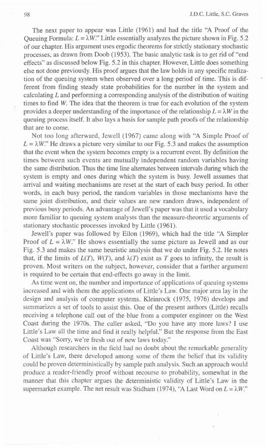
Let N denote the number of customers that shop on a particular day. Suppose thatwe keep track of when customers arrive and when they depart from the store. Thenwe can define and create two processes, one for the arrivals and the other for thedepartures. We define time t =0 to correspond to the opening at 7 AM, and timet = 16 to be the store closing at 11 PM, 16 h later.

We let N(t) denote the cumulative number of arrivals to the store by time t. Thus,as we start the day with zero customers, we have N(O)=0; as we assume a total ofN customers arrive during the day, we have N(16) = N. The cumulative arrivalsincrease in a stair-case fashion, as shown in Fig. 5.3, over 0 < t < 16.

In similar manner we define D(t) to denote the cumulative number of depar-tures from the store by time 1. Again, we have D(O) = 0, D(16) = N, and thecumulative departures increase in a stair-case fashion over the time interval0 < t < 16; see Fig. 5.3.

We note that at all time instants we have N(t) ~ D(t), as the number of departurescan never exceed the number of arrivals. Indeed, the difference between the twocumulative processes is the number of customers in the supermarket at time t:

L(t) =N(t) - D(t).

With this observation we can determine the average number in the supermarketover the course of the day from the following integral:

Q5.aE:J

Z

Q5

E0en:J0

s) S3 S4 c) TimeC2 C3S2

Fig. 5.3 Cumulative arrivals to and departures from a system, for example, the supermarket

90 J.D.C. Little, S.c. Graves

1 1=16

L=-x f (N(t)-D(t))dt.16 1=0

(2)

To model the average time in the supermarket for each customer is a bit moreinvolved. We define {Sl,S2' ... SN} to be the sequence of arrival or start times forthe N customers, where s. denotes the start time for the jth arriving customer. WeJ

define {Cj ,C2 ' ...CN}to be the sequence of departure or completion times for the Ncustomers, where c. denotes the completion time for the jth arriving customer. Thus,J

the time in the supermarket for the jth arriving customer is W.=C.- s.. AveragingJ J J

this over all the customers gives:

1

(

N N

)W=-x LCj- LSj .

N j=1 j=1

(3)

To compute (3) we shall develop an equivalent expression based on thegeometry in Fig. 5.3. Let us define {CI,C2,...CN}to be the sequence of depar-ture or completion times for the N customers, where cj denotes the completiontime for the jth departing customer. Since customers need nOt exit the store inthe order that they arrive, we shall often have c. =Fd. However, the sequence

I 2 N" . .J{c , C ,..., C } IS Just a permutatIOn or reordenng of the sequence {c I ' C2 ,...CN} as the departure time for each customer must appear exactly once ineach sequence.

As shown in Fig. 5.3, we can define the jth wait time as W =d - S., equal to theJ

difference between the departure time for the jth departing customer and the starttime for the jth arriving customer. Now let us consider the average of thesewait times:

1 N 1

(

N N

)-xLWj=-x Lcj-LSj .N j=l N j=l j=l

N N

But this will equal W given by (3), since LCj = Lcj. Hence we conclude thatj=l j=l

1 N 1

(

N N

)W=-xLwj=-x Lcj-LSj'

N j=l N j=l j=]

(4)

Now we need to relate our expression for L, given by (2) to our expression forW, given by (4). From the geometry in Fig. 5.3, we observe the followingequivalence:

1=16 N

f (N(t)-D(t))dt= IWJ.1=0 J=l

(5)

5 Little's Law 91

That is, on each side of the equation, we have an expression for the area between thecumulative anivals and the cumulative departures. On the left side we compute the areaby integration over time of the function that tracks the number in the system; on theright side we compute the area by summing up the time in system for N customers.

From (2), (4) and (5), we can now write Little's Law for the supermarket:

1 (=16 1 N NL=-x f (N(t)-n(t»)dt=-xLWj =-xW.

16 (=0 16 j=1 16(6)

N

We recognize 16to be the arrival rate in customers per hour for the particular

day, and we define A= N ; thus we have (6) in its familiar form, L =Itw.16 -.

With this simple example we have shown that Little's Law can be true over afinite time window (16 h) with nonstationary arrivals and with no notion of anysteady state for the system in question. On reflection, there were two essential con-ditions for this result:

. Boundary conditions-we specify the finite time window to start and end withan empty system. This was a natural condition for the supermarket, and indeed,would be common for many service systems.. Conservation of customers-we assume that all arriving customers will eventu-ally complete service and exit from the system; there are no lost customers, sothat the number of arrivals equals the number of departures. Again, this is a validassumption for many systems of interest.

We really needed nothing else beyond these conditions in order to establish thelaw in our case. We have no assumptions about N, the number of customers;indeed, all the equations hold true for any N, e.g., for N = 1. We have no assump-tions about the process for arrivals, or about how customers are serviced withinthe store. There might be a long period of no arrivals followed by the arrival ofseveral busloads of customers; there might be periods of no service completions,say, if all the cash registers stopped working for an hour. The only conditions areas stated above: we need to start and end with an empty system and we need toconserve customers.

Notice that our formula is exact, but after the fact. In other words, we cannotcomplete our calculation until the supermarket door shuts. This is not a complaint.It merely says that we are observing and measuring not forecasting. Another pointto mention is that the numbers will be different each day because of different setsof shoppers on different days of the week, the weather, holidays, and other changesin the store's internal and external environment. Nevertheless, the relationshipL = A."f. as measured for that day, will be exact and the ability to measure two ofthe parameters and deduce the third still holds.

92 J.D.C. Little, S.c. Graves

Further Discussion of "Average"

Little's Law holds exactly, but let us examine further what we mean by "average"wait, queue, and arrival rate. We have no probability distributions and so these are notexpected values. Looking at the derivation of the result, we see that we are talkingabout everyday sample averages in the case of waits and arrival rates and finite timeaverages in the case of queues. So Little's Law here shows us an exact relation amongsample and time averages. Next, consider a customer segment at the Sweet & Sour

supermarket that consists of men with children in strollers. We can compute sample: or time averages for their arrival rate, time in store, and number in store. Little's Law

will hold exactly. Therefore, Little's Law is true for these averages for any identifiablesegment. To use the relationship in practice, it will be necessary to collect dataobserving how many people of the target segment enter the store during the day.

To summarize, Little's Law is robust and remarkably general for queuing sys-tems for which a finite window of observation starts and stops when the system isempty. Interpretation of the area between cumulative arrivals and cumulative depar-tures permits an analytic argument that Little's Law is exact despite possibly non-stationary arrival and service processes. What we have discussed here turns out tobe the tip of a fascinating mathematical iceberg that has been developed in recentyears, called sample path analysis of queuing systems. An adequate discussion ofit is beyond the scope of this chapter but the interested reader is referred to the bookof EI-Tahaand Stidham(1999). .

Evolution of Little's Law in Operations Management

Over the past 15 years or so, Little's Law has played an increasingly important rolein the teaching and practice of operations management. However,the law is usuallystated in a modified format to emphasize its applicability to operations. Forinstance, we cite as an example the very successful textbook of Hopp and Spearman-(2000) who refer to Little's Law as a "... an interesting and fundamental, relation-ship between WIP, cycle time and throughput." They go on to state the law as

TH = WIPCT '

(7)

where they define throughput (TH) as "the average output of a production process(machine, workstation, line, plant) per unit time," work in process (WIP) as "theinventory between the start and end points of a product routing," and cycle time(CD as "the average time from release of a job at the beginning of the routing untilit reaches an inventory point at the end of the routing (that is, the time the partspends as WIP)." They note that cycle time is also referred to as flow time, through-put time, and sojourn time, depending on the context.

5 Little's Law 93

We easily see that (7) is equivalent to Little's Law with TH =Il,WI?=LandCT= W. However, there is a more fundamental difference in that the law is stated interms of the average output or departure rate for the system, rather than the arrivalrate. This reflects the perspective of a typical operating system, especially a manu-facturing operation. Output is a primary attribute of any manufacturing system,since it is nominally its raison d'etre. As stated, we see that any increase in outputrequires either an increase in work-in-process inventory or a reduction in cycle timeor both.

Furthermore in many contexts, the output rate is determined exogenously and isgiven to the manufacturing system; it reflects actual sales and/or a forecast of sales.The manufacturing system must then manage its operations to achieve this outputrate. It will need to determine how to release work to the operation so as to meetthe output target. In effect, the arrival process is endogenous. The operations man-ager decides the arrivals to the system based on the desired outputs. There is exten-sive research in the operations literature on how best to set the work release (orarrival process) to achieve the output targets. The best policies are dynamic policiesthat depend on the state of the manufacturing shop, e.g., depend on thework-in-process. .

Our originaldevelopmentof Little's Law assumesa stablesystemwith a stationaryarrival process; as discussed above, we cannot assume a stationary arrival processfor the typical context in which we might apply (7). Thus, we ask what conditionsare necessary for (7) to be valid. At a minimum we must have conservation offlow. Thus, the average output or departure rate (TH) equals the average input orarrival rate (A). Furthermore, we need to assume that all jobs that enter the shopwill eventually be completed and will exit the shop; there are no jobs that get lostor never depart from the shop. In addition, we need some notion of systemstability. We consider two possibilities, as this issue raises another importantconsideration.

First, we might assume that the shop will occasionally empty, i.e., WI? = O.Then, as with the supermarket example, we will see that Little's Law holds exactlybetween any two time instances at which the shop is empty.

However, in many mapufacturing systems, the WI? never drops to zero. In somecontexts, this occurs for behavioral reasons; as the WI? decreases, the shop naturallyslows down so as to not run out of work. The shop adjusts its service rate dynami-cally so as to keep from driving the WI? to zero. In other contexts, there might bean explicit control rule that maintains some target level or range of WI? Forinstance, a very effective control policy is the so-called CONWIP policy that main-tains an absolutely constant level of WI? (Hopp and Spearman, 2000); that is, thecontrol rule releases one unit of new work to the system whenever one unit of workcompletes processing and exits the system. In either case, Little's Law applies, atleast as an approximation, as long as we select a time interval that is long enoughfor two conditions to hold.

First, we need the size of the WI? to be roughly the same at the beginning andend of the time interval so that there is neither significant growth nor decline in thesize of the WI?

94 J.D.C. Little, S.c. Graves

Second, we need some assurance that the average age or latency of the WI? isneither growing nor declining. We have previously assumed that all jobs that enterthe shop will eventually be completed and will exit the shop. But if the WI? neverdrops to zero, it is possible for the jobs to be getting older or younger, in which casethe law does not hold.

To illustrate the problem, consider a doll store that offers a line of internationalfolk dolls. Each doll is adorned with traditional folk clothes from a particularcountry. The artist who produces the dolls gives each doll a distinctive hat inone of 10 different colors, which span the rainbow; the choice of color iscompletely at random. So, sometimes the Irish folk doll has a green hat, andsometimes a red hat. The store stocks 100 of these dolls so as to have a rich

. assortment of dolls from which to choose; whenever it sells a doll, the storeimmediately obtains a replacement from the supplier so as to maintain its in-storestock at 100 dolls. The supplier chooses the replacement'doll at random fromits supply.

Demand for the dolls has been quite good, as customers appreciate the artistryand novelty of the dolls. Indeed, the dolls sell consistently at a rate of about two perweek. However, customers have a subtle but strong subconscious dislike for dollswith mauve hats. Dolls with mauve hats seldom sell; indeed, these mauve-hat dollssell at a rate of about one every 2 years.

A naIve application of Little's Law might assume a doll arrival rate, equal to thedemand rate, A =2 per week and an average number in system L =100 dolls, andthen conclude that the average time in the store for a doll is W=50 weeks. However,this is not likely to be an accurate estimate over any moderate time interval, like afew years. Suppose we start with none of the hundred dolls having mauve hats.Every time we sell a doll there is a 1 in 10 chance that it will be replaced with adoll with a mauve hat, as the artist has 10 colors from which to choose. Since thesemauve-hat dolls sell much, much less frequently than any other doll, the mix ofdolls will gradually change over time. Indeed, the number of mauve-hat dolls in thestore grows by about 10 dolls per year. Dolls without mauve hats make up a smallerpercentage, but continue to sell at a rate of two per week; the time in system forthese dolls actually shrinks as they make up a smaller percentage of the storeassortment.However,the dolls with mauvehats do not sell andjust accumulate moreand more waiting time. Hence, the average age of the dolls in the store's assortmentcontinues to grow older until at some point, the entire assortment has mauve hats.As a consequence, we cannot apply Little's Law during this transient period.

For instance, suppose we observe the system for 5 years, and then use Little'sLaw to estimate W = L/A = 100/2 = 50 weeks; this estimate overstates the actualtime in system for those dolls that have sold. Over the first 5 years, the number ofmauve-hat dolls in the store grows from zero to about 50. As a consequence theactive inventory, namely the dolls without mauve hats, drops from 100 to about 50.These dolls stay in the system, on average, less than 50 weeks, whereas the mauve-hat dolls just sit and get older. Of course, if we extend the time interval, in 10 yearsthe entire assortment becomes mauve and the demand rate falls to one doll every 2years; eventually (about 200 years) the mauve inventory turns over and Little's Law

5 Little's Law 95

will now apply. Presumably, the store would recognize the trend a bit earlier and dosomething about it! Nevertheless, the example shows how Little's Law might nothold over some time interval during which the average age of the WI? or queue ischanging.

A quite different approach to the problem of nonzero WIP is motivated by whatwe learned in the supermarket problem. There we noted that Little's Law appliesindependently to each customer segment, but we have to be able to identify thecustomers in each segment and collect data on them.

So, in the case of non-zero WIP (or, actually, any existing WIP!), we can ignoreall of it and focus on a group of new items, which, for example, might be coloredblue. The system starts empty of blue items, even though it may be cluttered withothers. We count blues as they enter the system (the rate may be controlled if wewish-stationarity is not required). The observations we make depend on what wewanUo learn and what is easy to measure. Suppose we want to observe and processN blue items. And suppose we want to know the cycle time CT = W, the averagetime a blue item spends in processing. At regular intervals we take an inventory ofblues so that we can estimate WIP = L (for blues only) by simple averaging.

Eventually all N leave, say at T and so the average arrival rate is A=TH =NIT. ThenCT =W can be calculated by Little's Law. The underlying theory is exact, althoughwe have introduced some sampling error in estimating the blue WIP. However, thisis something we can control by putting whatever resources we think are worthwhileto reduce it.

Alternatively, we might have a way of determining blue cycle time CT = Wexactly and wish to know the average inventory of blue items, i.e., the blue WIP = L.This is the case in the followingexample. .

Consider a toy manufacturer that contracts with a third party logistics firm, 3PL,to handle its on-line business. The toy manufacturer will supply inventory to 3PL tofill orders. When the toy manufacturer receives an order on-line, it will instruct 3PLto fill it.

The toy manufacturer pays 3PL to provide this service. The contract termsdepend on two factors: the number of orders shipped and the amount of inventoryspace occupied by the t~ys at 3PL. The toy manufacturer pays 3PL $10 for everyorder that is shipped and $0.03 per day for each unit in inventory.

At the start of each month, the toy manufacturer ships a batch of toys to 3PL.These toys typically sell out within the month, but not always. For accounting rea-sons, the toy manufacturer insists that 3PL submit an invoice for its services foreach batch of toys. Hence, 3PL waits until the entire batch has been sold before itcan finalize an invoice. In preparing the invoice 3PL can easily determine theshipping-cost component, as it just depends on the number of toys in the batch.However, 3PL is less clear about how to account for how much inventory space isattributable to a batch of toys. One approach would be to count its inventoryeach day.However, it would be quite difficult to track the inventory associated with a partic-ular batch since the toys from all batches, as well as from other suppliers, are storedtogether in one section of the warehouse. Thus, it would be cost prohibitive to doan inventory count each day.

96 J.D.C. Little, S.c. Graves

A much simpler approach is to use Little's Law. Suppose that whenever 3PLreceives a batch of toys, it records the arrival date for each toy. 3PL can alsorecord the date at which the toy is shipped, and hence obtain the time in systemfor each toy.

For instance, if there were an RFID tag attached to each toy, then 3PL can easilyrecord these transactions with RFID readers at its shipping docks. Thus, 3PL knowsthe wait times W. for i = 1,2, .. .N, where W.is the difference between the ship timeand receipt time 'for the ithtoy and N is the 'number of toys in a batch. The averagewait time for the batch is

1 N

W=-L~'N i=l

If it takes T days to sell the batch of N toys, then the average arrival rate for thebatch is

'A=NT'

By Little's Law we now can find the average inventory attributable to thisbatch:

I N

L='AW=-L~'T i=l

Since L represents the average inventory over a period of T days, 3PL willcharge the toy manufacturer for Lx T unit-days of inventory storage, at $0.03 perunit-day.

Concluding Remarks

We have given a variety of examples showing the kinds of situations where Little'sLaw can usefully convert an estimate of an average queue into an estimate of aver-age waiting time and vice versa when one may be relatively easy to measure andthe other not.

We have also briefly examined how Little's Law has been used in operationsmanagement. Here we observe that a different terminology and set of symbols isusually adopted. Operations managers are concerned with their throughput raterather than an arrival rate; their queue length is usually WI?, their wait time istermed cycle or flow time. We also discussed two differences in orientationsbetween the use of the law in operations management and its original derivationandapplication:

5 Little's Law 97

. For operations management the law is often expressed in terms of output ratesrather than arrival rates.Furthermore, the arrivalprocess to most operatingsystemsis not a stationary process, and, indeed, may be controlled.

. Many operating systems are never empty. That is, the number in the system orWIP is always positive.

In each case we see that Little's Law can apply, albeit with some required condi-tions and thoughtful attention to the goals of the application.

Historical Background

We trace the evolution of Little's Law from the early days of queuing theory inoperations research and management science to our own chapter in this book. .

The earliest paper we have found that makes use of Little's Law simply assumesit to be true. Cobham (1954), in an article on priority queues, writes, "... it is suffi-cient to observe that the expected number of units of priority k waiting to be servicedis AkWk,where Wkis the expected wait for a unit of priority k." (Akis the arrival rateof priority k items.)

We attribute the explicit formula "L = AW' to Philip Morse and his book,Queues, Inventories and Maintenance, (Morse, 1958). He does not give the lawa name but simply talks about "the relation between mean number and meandelay." In Chap. 7 he proves the relationship for a single channel queuing sys-tem having Poisson arrivals and a service time distribution of the general classknown as k-Erlang. The proof of L =AW is, in a certain sense, incidental to hismain task of solving for the steady-state joint probabilities of the number ofitems in the system and the stage of item in service. Using the fairly standardapproach of describing the system with a set of differential equations, Morsesolves the system by building a two variable generating function of the desiredjoint probabilities. One variable relates to the number of items in the systemand the other to the stage of the item in service. The generating function canthen be used rather e,\sily to find both Land W. Examination shows that Land W differ only by the constant of proportionality A. This is a nice piece ofanalysis of the particular system, but it does not readily suggest a route togreater generality.

Morse was clearly interested in the general case. After the above analysis hewrote, "we have now shown that... the relation between the mean number and meandelay is via the factor A, the arrival rate: L = AWand We will find, in all theexamples encountered in this chapter and the next, for a wide variety of service andarrival distributions, for one or for several channels, that this same relationshipholds. Those readers who would like to experience for themselves the slipperinessof fundamental concepts in this field and the intractability of really generaltheorems, might try their hand at showing under what circumstances this simplerelationship between Land W does not hold."

98 lD.C. Little, S.c. Graves

The next paper to appear was Little (1961) and had the title "A Proof of theQueuing Formula: L =AW."Little essentially analyzes the picture shown in Fig. 5.2of our chapter. His argument uses ergodic theorems for strictly stationary stochasticprocesses, as drawn from Doob (1953). The basic analytic task is to get rid of "endeffects" as discussed below Fig. 5.2 in this chapter. However,Little does somethingelse not done previously. His proof argues that the law holds in any specific realiza-tion of the queuing system when observed over a long period of time. This is dif-ferent from finding steady state probabilities for the number iri the system andcalculating L and performing a corresponding analysis of the distribution of waitingtimes to find W. The idea that the theorem is true for each evolution of the systemprovides a deeper understanding of the importance of the relationship L =AW in thequeuing process itself. It also lays a basis for sample path proofs of the relationshipthat are to come.

Not too long afterward, Jewell (1967) came along with "A Simple Proof ofL = AW." He draws a picture very similar to our Fig. 5.3 and makes the assumptionthat the event when the system becomes empty is a recurrent event. By definition thetimes between such events are mutually independent random variables havingthe same distribution.Thus the time line alternatesbetween intervalsduring which thesystem is empty and ones during which the system is busy. Jewell assumes thatarrival and waiting mechanisms are reset at the start of each busy period. In otherwords, in each busy period, the random variables in those mechanisms have thesame joint distribution, and their values are new random draws, independent ofprevious busy periods. An advantage of Jewell's paper was that it used a vocabularymore familiar to queuing system analysts than the measure-theoretic arguments ofstationary stochastic processes invoked by Little (1961).

Jewell's paper was followed by Eilon (1969), which had the title "A SimplerProof of L = AW." He shows essentially the same picture as Jewell and as ourFig. 5.3 and makes the same heuristic analysis that we do under Fig. 5.2. He notesthat, if the limits of L(T), W(T), and A(T)exist as T goes to infinity, the result isproven. Most writers on the subject, however, consider that a further argumentis required to be certain that end-effects go away in the limit.

As time went on, the number and importance of applications of queuing systems. increased and with them the applications of Little's Law. One major area lay in the

design and analysis of computer systems. Kleinrock (1975, 1976) develops andsummarizes a set of tools to assist this. One of the present authors (Little) recallsreceiving a telephone call out of the blue from a computer engineer on the WestCoast during the 1970s. The caller asked, "Do you have anymore laws? I useLittle's Lawall the time and find it really helpful." But the response from the EastCoast was "Sorry, we're fresh out of new laws today."

Although researchers in the field had no doubt about the remarkable generalityof Little's Law, there developed among some of them the belief that its validitycould be proven deterministically by sample path analysis. Such an approach wouldproduce a reader-friendly proof without recourse to probability, somewhat in themanner that this chapter argues the deterministic validity of Little's Law in thesupermarket example. The net result was Stidham (1974), "A Last Word on L = AW."

5 Little's Law 99

However, as he pointed out in a later review article (Stidham, 2002), it was not thelast word at all because the research potential of sample path analysis for queuingand other applications has ramifications far beyond Little's Law. Many results ofthis sort appear in a book by Stidham and a colleague: (EI-Taha and Stidham,1999): Sample-Path Analysis of Queueing Systems.

Over the past few years, Little's Law has become increasingly important inoperations management. The notation and type of thinking are different, but appli-cations are growing in number and importance. The goal of this chapter has beento facilitate such applications by providing illustrative examples, especially onesthat explore new territory.

A Note of Personal History (Little)

How did a sensible young PhD like me get involved in a crazy field like this? From1957-1962, I taught operations research at the Case Institute of Technology inCleveland (now Case Western Reserve University). I was asked to teach a courseon queuing. OK. Initially I used my own notes, but when Morse (1958) came out,I used his book extensively. Queuing was taken by most of the OR graduate stu-dents and, indeed, one of these, Ron Wolff, went on to become a first class queuingtheorist (Wolff 1989). One year we were at the point when we had done the basicPoisson-exponential queue and moved through multi-server queues, and some othergeneral cases. I remarked, as many before and after me probably have (and Morsedoes), that the often reappearing formula L =AW seemed very general. In additionI gave the heuristic proof that is essentially Fig. 5.2 at the beginning of this chapter.After class I was talking to a number of students and one of them (Sid Hess) asked,"How hard would it be to prove it in general?" On the spur of the moment, I oblig-ingly said, "I guess it shouldn't be too hard." Famous last words. Sid replied, "Thenyou should do it!"

The remark stuck in my mind and I started to think about the question from timeto time. Clearly there was something fundamental going on, since, when youdraw the picture you do not really seem to need any detailed assumptions aboutinterarrival times, service times, number of servers, order of service, and all theother ingredients that go into the panoply of queuing models. You only seemed toneed a process that goes up and down in unit amounts and some guarantee of steadystate and conservation of items. In addition, because I could see there were endeffects in the picture, there needed to be a way to get rid of them in the limit. Itseemed to me I was in the general arena of stationary.stochastic processes. I am nota mathematician by training, and so I bought copies.of measure theoretic stochasticprocess books like Doob (1953), which mentioned stationary processes and ergodictheorems.

My family's habit at the time was to go to Nantucket in the summer where mywife's family had a small summer house. We would load our children in a stationwagon, drive to Woods Hole, take the ferry, and spend a couple months away from

100 J.D.C. Little, S.c. Graves

the world. Since the beach was the baby-sitter, I was able to split off solid blocksof time to work on research as a good assistant professor should. (I wish I could dothat today!) I always brought a pile of books and projects with me. L ='AWwasoneof them. I soon ran into problems that required more than looking up theorems inmy new books, but I worked out approaches to the road blocks and eventually wroteeverything up, giving it my best shot. I sent the paper off to Operations Research.It was accepted on the first round.

Nevertheless, I had learned my lesson. I decided that Borel fields and metrictransitivity were not going to be my career and retired from queuing. That was in

. 1961.My retirementhelduntil 2004whenI was accostedby emailand in personat an INFORMS meeting by Tim Lowe. Even then, as he will tell you, I resisted

. re-entrapment, saying, "I don't know anything about OM and I haven't looked atL = 'AW for 40 years." Being always susceptible to a new challenge and, moreimportantly, thanks to much help from Steve Graves, who really does know OM,I took a run at holding up my end of the chapter. It has been a wonderful experienceand I have learned much. Now I need to find ways to use it.

References

Cobham, A. (1954) "Priority Assignment in Waiting Line Problems," Operations Research, 2, (1)(Feb.), 70-76.

Doob, J. L. (1953) Stochastic Processes, John Wiley, New York.Eilon, S. (1969)"A Simpler Proof of L =AW,"Operations Research, 17, (5) 915-917.El-Taha, M. and S. Stidham (1999) Sample-Path Analysis of Queueing Systems, Kluwer Academic,

Boston MA.

Hopp, W. J. and M. L. Spearman (2000) Factory Physics: Foundations of ManufacturingManagement, 2nd (ed.), IrwinlMcGraw Hill, New York, NY.

Jewell, W. S. (1967), "A Simple Proof of L =AW," Operations Research, 15, (6) 1109-1116.

Kleinrock, L. (1975) Queueing Systems, Volume I: Theory, A Wiley-Interscience Publication,New York.

Kleinrock, L. (1976) Queueing Systems, Volume II: Computer Applications, A Wiley-IntersciencePublication, New York.

Little, J. D. C. (1961) "A Proof of the Queuing Formula: L = AW," Operations Research, 9, (3)

383-387.

Little, J. D. C. (1992) "Are there 'Laws' of Manufacturing," Manufacturing System.s: Foundations

of World-Class Practice, edited by 1. A. Heim and W. D. Compton, National Academy Press,Washington, D.C., 180-188.

Morse, P. M. (1958) Queues, Inventories and Maintenance, Publications in Operations ResearchNo.1, John Wiley, New York.

Stidham, S., Jr. (1974) "A Last Word on L = AW,"Operations Research, 22, (2) 417-421.Stidham, S., Jr. (2002) "Analysis, Design, and Control of Queueing Systems," Operations

Research, 50, (1) 197-216.

Wolff, R. W. (1989) Stochastic Modeling and the Theory of Queues, Prentice-Hall, Inc., EnglewoodCliffs, New Jersey.