chapter 5: magnetostatics, faraday's law, 5.1 introduction and
TRANSCRIPT

Chapter 5: Magnetostatics, Faraday’s Law,
5.1 Introduction and DefinitionsQuasi-Static Fields
3 3
We begin with the law of conservation of charge: Qd x d d x J J a
5.1 Introduction and Definitions
da, J
B
conservation0 (5 2)f h
v vQt td x d d x
J J a
J
arbitrary volume
0 (5.2)of charge
Magnetost
t J
atics is applicable under the static condition. Hence,
0 and (5.2) gives 0 [for magnetoststics] (5.3)
Assuming a magnetic force is experienced by charge movingB
tq
J
F Assuming a magnetic force is experienced by charge movingat v
B qFelocity , we define the magnetic induction by the relation:
B q v B
F v B ,which is consistent with the definition in (5.1).
B q F v B
1
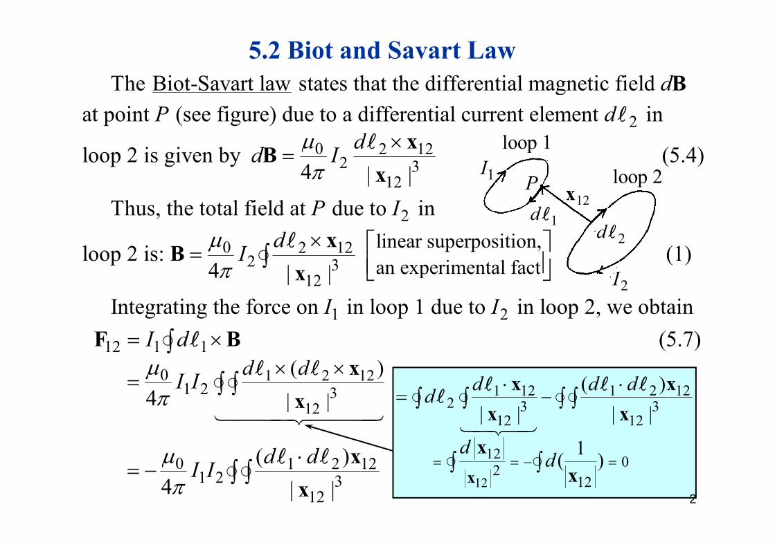
5.2 Biot and Savart LawThe Biot-Savart law states that the differential magnetic field dB
loop 1 2
0 2 12
The Biot Savart law states that the differential magnetic field at point (see figure) due to a differential current element in
l 2 i i b
dP d
dd I
B
xB
(5 4)
1I
dx
p
loop 2 P12
0 2 122 3
12loop 2 is given by
4 | |
d IBx
2
(5.4)
Thus the total field at due to inP I
I
1d2d
2
0 2 122 3
linear superposition,an experimental fact
Thus, the total field at due to in
loop 2 is: (1)4 | |
P IdI xB
x
2I12an experimental fact4 | |
Integrating the x
1 2 force on in loop 1 due to in loop 2, we obtain(5 7)
I II dF B
1 12 1 2 122
( )d d dd
x x
1 2 123
12 1 1
01 2
( )| |
(5.7)
4
d d
I d
I I xF B
2 3 312 12| | | |
d x x
12 01( )
dd
x
312
| |4x
0 1 2 12( )
d d x
1202
12( )d
x x 0 1 2 121 2 3
12
( ) 4 | |
d dI I x
x
2

x x x
5.3 Differential Equations of Magnetostatics and Ampere’s Law
12 1 2 x x x
1x2x
B
2d
d xGauss Law of Magnetism :
and Ampere s Law
cross section 2
2I02
3
0 2 123
124 | | Rewrite (1): dI
x
xB
cross sectionof wire
31 2 2 2 2
30 03
Change to , to , and let , we obtain1 ( ) ( ) ( )
I d da d d x
d x
x x x x J Jx xB x J x J x
3d x3( ) ( ) ( )
4 4 | || | x xx x
B x x3
1| || |
x xx xx x a a a
30 ( ) 1 [ ( )]4 | | | |
d x
J x J xx x x x
xx
( )J x
| || |x x
030
| | | | ( ) (5.16)
4 | |d x
J xx x
0
operates on x| |
0 [Gauss B law of magnetism] (5.17)
p
3

Rewrite (5.16):Ampere's Law :5.3 Differential Equations of Magnetostatics and Ampere’s Law (continued)
30
Rewrite (5.16): ( ) ( )
4 | |d x
Ampere s Law :J xB xx x
30
31 1| | | |
( )| |
( ) ( )[ ]
d x
d x
J x
x x x x
x x
J x J x
0 ( ) 3
| | ( )
d x
J x
B x| | | |
31| |
( )3 31
( ) ( )[ ]
( )
( )
d x
d d
J x
x x x x
x xJ x
2 30
| |
( ) 3 10
4
d x
x x
J x
( )3 31| | | |
0 0
( ) d x d x J x
x x x xJ x
n
2 30
4 ( )
( ) 3| |
1| |( )
4[ ]d xd x
x x
J xx x x xJ x
2( ) ( ) a a a
da
narbitrary
loop
( )
0 ( ) ( ) (5.22) da da
B x J x B n J n
( ) ( ) a a a
dloop0
(through the loop)
Ampere's lawd I
da da
BB n J n
a much more elaborate
0, Ampere s law
d I B a much more elaborate
representation of the Biot-Savart law (5.25) 4
( ) J x5.4 Vector Potential
30 ( )| |
Rewrite (5.16): ( ) 4
(5 27)
d x
J xx x
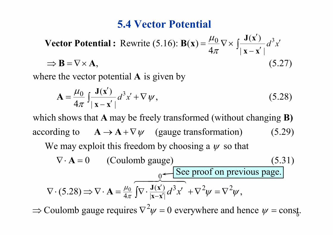
Vector Potential : B x
B A , (5.27)where the vector potential is given by
B AA
( ) J x 30 ( )| |
, (5.28)4
which shows that may be freely transformed (without changing
d x
J xx x
A
A B)which shows that may be freely transformed (without changing according to (gauge transformat
A B)A A ion) (5.29)
W l it thi f d b h i th t We may exploit this freedom by choosing a so that 0 (Coulomb gauge) (5.31)
A
See proof on previous page
0 ( ) 34 | | (5.28) d
J x
x xA
02 2 ,x
See proof on previous page.
4 | | x x2Coulomb gauge requires 0 everywhere and hence const.
5

5.4 Vector Potential (continued)
0 Rewrite:
B J B A
02
0
( )
A J
A A J0
2
( ) Choose the Coulomb gauge ( 0)
(5 31)
A
A J0 (5.31)
A J
30 ( ) (5.32)4
d xJ xA
| |( )
4:
Notex x
(5.32) is valid in unbounded (infinite) space, i.e. the volume ofintegration must include all currents. If there is a boundary surface, the currents on the boundary must be accounted for by applicationthe currents on the boundary must be accounted for by applicationof boundary conditions (See example in Sec. 5.12.) 6

A Comparison of Electrostatics and Magnetostatics :5.4 Vector Potential (continued)
D fi i i f Magnetostatics
B Electrostatics
A Comparison of Electrostatics and Magnetostatics :
J
x
Definition of : B q
BF v B
x
Definition of : E q
EF E
x x
Biot-Savart law:
x x
Coulomb's law: 1 ( )( ) 30
3( ) ( )4 | |
d x
x xB x J xx x
33
0
1 ( )( )( )4 | |
d x
x x xE xx x
00
B B J
0 0
E E
00Gauss's Law Ampere's law
d d I B a B 0 0
G ' ld q d
E a E Gauss's Law Ampere's lawof magnetism
Gauss's law of electrostatics 7

5.6 Magnetic Field of Localized Current Distribution, Magnetic Moment
30
( ) d
Magnetic (Dipole) Moment : J xA 1 1 [ ( ) Ch 4]x x
Distribution, Magnetic Moment)()()( BACCABCBA
J
30
3 30
( )4 | |
1 1[ ( ) ( ) ]
d x
d x d x
Ax x
J x x x J x
3| |1 1 [Eq. (5), Ch. 4]
| | | |
xx x
x x x
x x
J
0
03
0
[ ( ) ( ) ]4 | | | |
d x d x
J x x x J xx x
Proved on next page31
2 [ ( )]d x x x J x
Proved on p.185 under the1. is localized
J03
3[ ( )]
| |
8d x
x x J x
x
Proved on next page.
within volume conditions: of integration2 0
J0
3
| |8If is far from source.4 | |
xm x x
x (5.55)
2. 0 J4 | | x31
2where ( ) [magnetic (dipole) moment] (5.54)I (5 54) i d fi d ith t t
d xN t i t f f
m x J xm : In (5.54), is defined with respect to a
Here, it Note point of reference.m
coincides with the origin of the coordinates ( 0). x 8

3: Prove the relation ( ) 0 under the conditions:Problem d x J x5.6 Magnetic Field of Localized Current Distribution, Magnetic Moment (continued)
0 and is localized within volume of integration.: Since 0 outside the volume of integration, we may extend Proof
J JJ
the3
volume of integration to without changing the integral value. ( ) )x x y y z zd x dx dy dz(J J J
J x e e e
3 Consider the -component first: ( )x x
xd x dy dz J dx
e J x( )
x xy
d
xJ
xJ
y dz x dx
xxJ
xJ
x dxx
3
0
( )yx zJJ Jx y zdy dz x dx
d
J
3 0 Similarly, the - and
components also vanish
x d xy
z
J The insertion of these 2 terms will notchange the value of the integral because
y JJ
3-components also vanish.
Thus, ( ) 0 z
d x J x&( ) 0 ( ) 0y zJ
y zJy zdy J dz J
9

( ): (used on p 185 and p 188)Anti symmetric unit tensor 5.6 Magnetic Field of Localized Current Distribution, Magnetic Moment (continued)
( ): (used on p.185 and p.188)0 , if two or more indices are equal1 if i t ti f 1 2 3
ijkAnti - symmetric unit tensor
i j k
(2)
1 , if , , is an even permutation of 1, 2,31 , if , , is an odd permutation of 1, 2,3
ijk i j ki j k
(2)
0 1 1 1E l
Levi-Civita symbol
112 123 132 312: 0, 1, 1, 1 ( ) , ( )
ji ijk j k i ijk kxk k
Examples
A B A
A B A
( )
j
i
j j j xjk jk
ijk j kxijkA B
A B
j ki
ijkA B
ijk k ijk jx xB A
iijk
j ki i
jA B
kij k jik jx xijkB A
( ) ( ) B A A B10

: plane loopExample 1of magnetic moment5.6 Magnetic Field of Localized Current Distribution, Magnetic Moment (continued)
Id
3
2 ( )
12 2
: plane loop
( ) I Example 1 of magnetic moment
d x d x J xm x
dax2 ( )
( ) (5.57)
is normal (by rig
areaI area
mm ht hand rule) to the plane of the loop is normal (by rigm ht hand rule) to the plane of the loop.
: a number of charged particlesi ti
Example 2 of magnetic moment
in motion ( )i i i
iq J v x x
angular momentumi i i iM L x v
31 12 2 ( )
2
i
ii i i i
i i i
qd x qM
m x J x x v L (5.58)i
(5.59)2
eM
Lif / / for all particles.i iq M e M
2M: total angular momentumL
11

5.6 Magnetic Field of Localized Current Distribution, Magnetic Moment (continued)
(valid far from the source)Dipole Field :
03| |
(valid far from the source)
Rewrite (5.55) : (5.55)4
m xx
Dipole Field :
A3 3 3
1 1 x x x
03
| |
| |
4
4
xxx
B A m
3 3 3
3 5
| | | | | |3 3
| | | |0
x x x
xx x
x x
x
0 00
| |4
[
x
x x x
0
]
x
| | | |
( is a constant.)m
03 3| | | | |
[4
x x xx x
m m
0
3 3| | |]
m m m
xx x
x x x
m m
( ) ( ) ( ) A B B A A B
0
0
3 3 3
| | | | | |
43x
x y zx y zm m m
x
x x x
e
( ) ( ) ( ) ( ) ( ) A B B A
0
0
53 | || |
43 ( ) magnetic dipole
xxm y z
xxx
n n m m (5 56) x03
( ) g p fie4 | |
x
(5.56)ld | |
nx
12
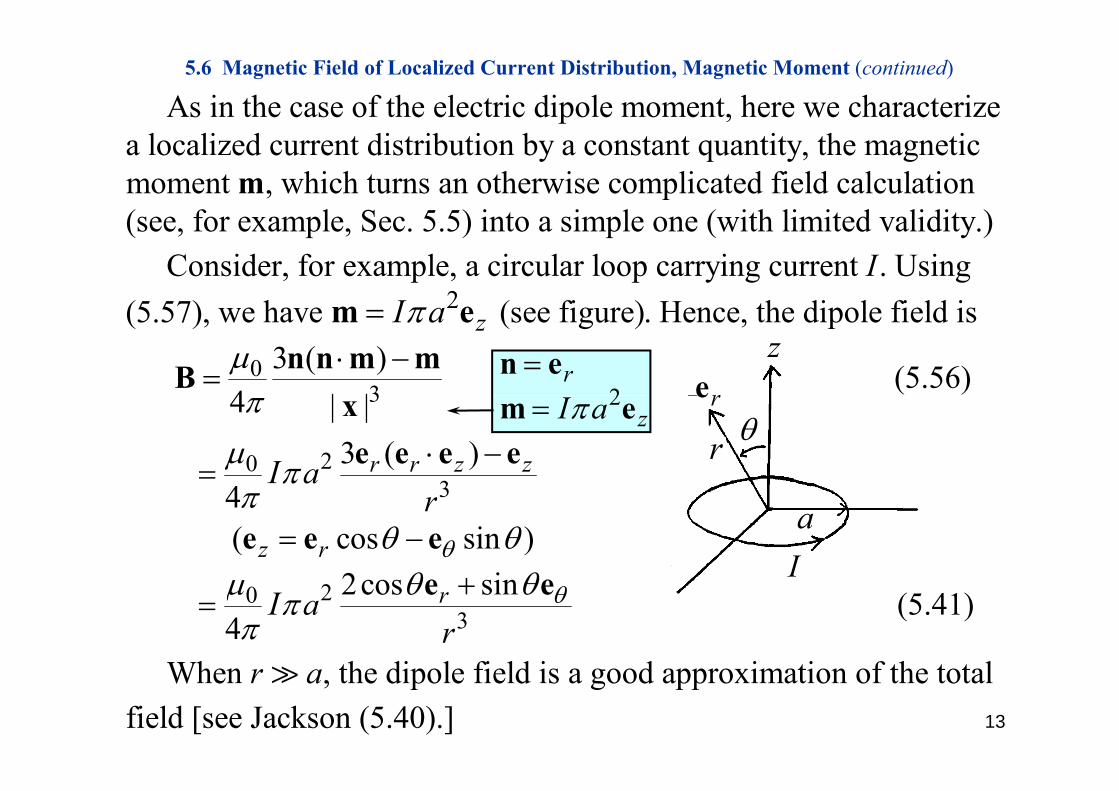
As in the case of the electric dipole moment, here we characterize5.6 Magnetic Field of Localized Current Distribution, Magnetic Moment (continued)
a localized current distribution by a constant quantity, the magnetic moment , which turns an otherwise complicated field calculm ation ( f l S 5 5) i t i l ( ith li it d lidit )
2
(see, for example, Sec. 5.5) into a simple one (with limited validity.) Consider, for example, a circular loop carrying current . Using(5 57) h ( fi ) H th di
II l fi ld i
rez
2(5.57), we have (see figure). Hence, the dipo zI am e0
3
le field is3 ( ) (5.56)
4 | |
n n m mB
2rn e
rre
3
203
4 | |3 ( ) r r z zaI
xe e e e
2zI am e
a
I
34 ( cos sin )
2 iz r
r
e e e I
203
2cos sin 4
rar
I
e e (5.41)
Wh th di l fi ld i d i ti f th t t l When , the dipole field is a good approximation of the total field [see Jackson (5.40).]
r a13

5.7 Forces and Torque on and Energy of a Localized Current Distribution in an External Magnetic Induction
3:
( ) ( ) (5 12)d x Magnetic Force in External Field
F J x B x
Current Distribution in an External Magnetic Induction
( ) ( ) (5.12) Expanding : [see lecture notes, Ch. 4, Appendix A, Eq. (A.4)]
d x F J x B xB
( ) (0) ( ) (0)B B B ( ) (0) ( ) (0) B x B x B This implies "After differention of ( ), set in results to 0," i.e.B x x
0 00
p ( )
( ) (0) ( ) ( ) ( )y zxx y z
x xxx B B x B x B x
3 3
(proved in Sec. 5.6)
( ) (0) ( ) ( ) (0)
0
[ ]d x d x
F J x B J x x B
3(p )
( ) ( ) (0) ( ),
d xU
J x x B m B
(5.69)See derivation on pp.188-189 , U (5.69)where potential energy. (5.72)U m B
See derivation on pp.188 189
14

:Magnetic Torque in External Field5.7 Forces and Torque… (continued)
3
3
( )
[ ( ) ( )] (5 13)
d x
d
g q
N x f x
J B 0
2
2[ ( )]
xx J x
3
(0) ( ) (0) (0)
[ ( ) ( )] (5.13)d x
B x B B
x J x B x
02 2
2
( ) ( )
2 ( )
x
x xJ x x J
x J x
( ) ( ) ( ) ( )
x 3
3 3
[ ( ) (0)]
[ (0) ] ( ) (0) ( )
d x
d d
J x B
B J B J
2 ( ) x J x
3 3
23 312
[ (0) ] ( ) (0) ( )
= [ (0) ] ( ) (0) [ ( )]
d x d x
d x d x
B x J x B x J x
B x J x B x J x 31
2 (0) [ ( )]d x B x J x 2 ( ) 0 ds x J x a[Using
]
the formula at thebottom of p.185, replacing
with (0).x B
is localized. 0 on surface
JJ
(0) m B (5.71)]with (0).x B
15

5.7 Forces and Torque… (continued)
A Comparison between Electric and Magnetic Potential Energy,
Potential energy Force Torque
A Comparison between Electric and Magnetic Potential Energy, Force, and Torque in External Field :
(4.24)
(5 72)
Potential energy Force TorqueU UU U
p E F N p Em B F N m B
Ep + (5.72)
Both and tend to orient along thepositive field direction under the action of
U U m B F N m Bp m
p
BmI
positive field direction under the action ofthe torque (see figures on the right). This results in a state of minimum potential
Ienergy. In this state, , whereas .
reducesenhances
p Em B
(1) How does a permanent magnet attract a piece of iron? :Questions
(2) How does it attract another permanent magnet? 16
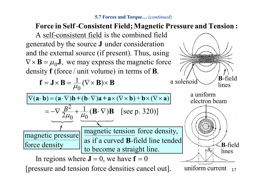
- Force in Self Consistent Field; Magnetic Pressure and Tension :5.7 Forces and Torque… (continued)
A self-consistent field is the combined field generated by the source under consideration
d h l (if )
; g
JTh iand the external source (if present).
0
Thus, using, we may express the magnetic force
density (force / unit volume) in terms of B J f B
01
density (force / unit volume) in terms of . ( )
f Bf J B B B
if
-field linesBa solenoid
2 12 ( ) B B B [see p. 320)] (3)
a uniformelectron beam( ) ( ) ( ) ( ) + ( ) a b a b + b a + a b b a
002 ( ) [ p )] ( )
magnetic pressure magnetic tension force density,
I i h 0 h 0J fB
-field linesB
magnetic pressure force density as if a curved -field line tended
to become a straight line.B
In regions where 0, we have 0 [pressure and tension force densities cancel out].
J funiform current 17

5.8 Macroscopic Equations, Boundary Conditions on B and HConditions on B and H
0
To be more general, we move thepoint of reference for from 0 to and write
Macroscopic Equations :m x x x0
0 03
0 0
p( ) ( )1 1 [See Sec. 4.1]
x x x xx x x x x x
x xJ
0
0 0
Sub. this relation into
x x
( ) J xHow about Jfree?
i h l if i l li dJ
0 30 ( )| |
[(5.32)]4
d x
J xx x
A
J
0x x0 x x
vanishes only if is localized within the volume of integration.
Jwe obtain
0x xx
30 0 0 0
30 0
( ) ( ) ( ) , (4)4 | | 4 | |
d x
J x m x x xA
x x x x
0
031
0 02
| |
where ( ) ( ) ( ) .d x m x x x J x18

To proceed, we consider the orbital motion of atomic/molecular5.8 Macroscopic Equations, Boundary Conditions on B and H (continued)
To proceed, we consider the orbital motion of atomic/molecularelectrons, which can collectively give rise to a permanent or inducedmagnetization (total magnetic moment / unit volume) given byM ( ) (5.76) i i
iNM x m
magnetic moment per type i moleculevolume density of
As will be shown in (5.79), a current density ( ) is associatedMJ
magnetic moment per type i moleculeaveraged over a small volume
volume density oftype i molecules
As will be shown in (5.79), a current density ( ) is associated with . In addition, there is also a current
MJM density due to the flow of
charges, which we denote by (Jackson denotes it by in freefree J JSec. 5.8). By the principle of linear superposition, we may write ( ) ( )
f
freeA x A x A ( ),M x( ) ( )free ( )where and are due to and , respectively.
( )
M
free M free M
f
A A J JJ x 30 ( )
Obviously, ( )4 | |
freefree d x
J xA x
x x 19

For , we have the expression for , but not yet for . SoM MA M J5.8 Macroscopic Equations, Boundary Conditions on B and H (continued)
3
, p , ywe approximate by the dipole term in (4).
( )
M M
M
M d x
A
J x ( ) ( ) m x x x0 ( ) ( )
4
M
Md xJ x
A x 0 0 03
0 03
( ) ( ) , | | 4 | |
h h t ( ) 0 b i f d f t
d
m x x xx x x xJ J3where we have set ( ) 0 because is formed of current
loops of atomic dimensions ( volume of integration). Under thiscondition is independent of the poin
M Md xJ x J
m t of reference becausecondition, is independent of the poinm31
0 02 0
t of reference because
( ) ( ) ( ) M d xm x x x J x
(5.54)3 31 1
02 2 ( ) ( ) (0).To represent by the dipole term we must have the
M M
M
d x d xx J x x J x mA x To represent by the dipole term, we must have the
dimension of the dipMA x
ole. So, we divide the source into infinistesimalvolumes. In each small volume , the dipole moment is , V VM, p ,which generates a small at given by MA x
20
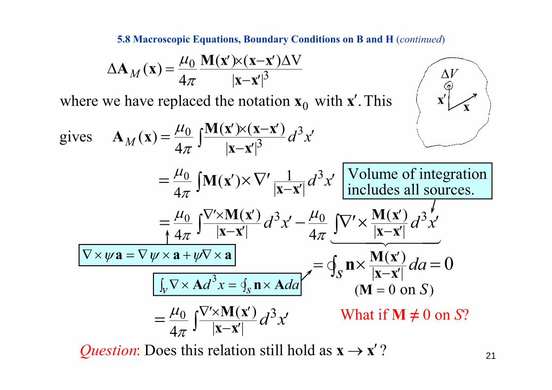
0 ( ) ( ) V M x x x5.8 Macroscopic Equations, Boundary Conditions on B and H (continued)
0
0
3( ) ( ) V
| | ( )
4where we have replaced the notation with . This
MM x x x
x xA x
x x x x
V
0
303
( ) ( )| |
p
gives ( ) 4
M d xM x x xx x
A x
x
0 3
| |
1| |4
4
( )
d x
x x
x xM x Volume of integrationincludes all sources.| |4
0 03 3( ) ( )
| | | |4 4
d x d xM x M x
x x x x
4( )
| |
4
0
dasM xx xn
S
a a a3
d x daA n A
0
( )
3
0 ( )
| |
on
4
S
d x
MM x
x x
v sd x daA n A
What if M ≠ 0 on S?| |4
Does this relation i: st ll
Questionx x
hold as ?x x 21

6.2 The Field of a Magnetized Object 6 2 1 B d C t
Griffith1/4
6.2.1 Bound CurrentsSuppose we have a piece of magnetized material (i.e. M is given). What field does this object produce?
The vector potential of a single dipole m is
r̂m2
0
4)(
rr
mrA
I th ti d bj t h l l t iIn the magnetized object, each volume element carries a dipole moment Md’, so the total vector potential is
d2
0 ˆ)(4
)(r
rrMrA
22
4 r

Vector potential and Bound CurrentsGriffith 2/4
Can the equation be expressed in a more illuminating form, as in the electrical case? Yes!
By exploiting the identity,ˆ1 r 2 2 2
1ˆ ˆ ˆ( )( ) ( ) ( )x y z x x y y z z
x y z
2
1rrr
2 2 2 3/ 2 2
( ) ( ) ( )ˆ ˆ ˆ( ) ( ) ( ) ˆ
(( ) ( ) ( ) )
y x x y y z zx x y y z z
x x y y z z
x y z rr
The vector potential is d)1()(4
)( 0
rrMrA
)()( AAA fffU i th d t land integrating by part, we have
)()( AAA fffUsing the product rule
)(1 M dd
11
])([)]([14
)( 0 rMrMrArr
How? See next page.
23add
]ˆ)([1
4)]([1
400 nrMrM
rr

Griffith 3/4
Gauss's law ( )S
d d E E a( ( )) ( )
Let
v S
v v
d d
v c c v
E v cLet , ( )
S S
d d
E v cv c a c v a
24Since is a constant vector, so ( )
v S
d d c v v a

Vector potential and Bound CurrentsGriffith4/4
add ]ˆ)([14
)]([14
)( 00 nrMrMrArr
44 rr
)(rMJ b ˆ)( nrMK b
With these definitions bound currents
currentvolume currentsurface
With these definitions,
add b
S
b KJrA
44)( 00
The electrical analogy
Sv rr 44
The electrical analogy Pbdensity charge volume
25ˆsurface charge density bσ P n

5.8 Macroscopic Equations, Boundary Conditions on B and H (continued)
Th ( ) ( ) ( )A A A
30
Thus, ( ) ( ) ( )( ) ( )
(5 78)
free M
free d x
A x A x A xJ x M x
20
(5.78)4 | |
For comparison, in Sec. 5.3, we have , (5.31)
d xx x
A J0p ( )
whic
30 ( )h has the solution: ( ) (5.32)
4 | |
d xJ xA xx x
In (5.31) and (5.32), represents the current due to both free and bound (atomic) electrons, whereas in (5.78) contrib
Jutions from
free and bound electrons are separated into two terms.
Comparing (5.78) and (5.32), we find that the bound electronsp g ( ) ( ),contribute to ( ) through a magnetization current density ( ) given
MA x J by , (5.79) MJ M
which is the macroscopic exhibition of the atomic currents.M
26

0 Hence, by separating free and bound electrons, ( ) ( ) B x J x 5.8 Macroscopic Equations, Boundary Conditions on B and H (continued)
0
0
y p g ( ) ( )[(5.22)] can be written ( ) (5.80)
Defining a new quantity called the magnetic field :
freeB J MH Defining a new quantity called the magnetic field :
H
01 Effects of the atomic , (5.81) currents are implicit in .
H B M H0 p
we obtain from (5.80) the macroscopic version of (5.22):
fH J (5 82) freeH J (5.82)Does have a physical meaning?: Question H
Diamagnetic Paramagnetic and Ferromagnetic Substances :
0
The counterpart of (5.81) in electrostatics is
Diamagnetic, Paramagnetic, and Ferromagnetic Substances :D E [(4.34)].
In Sec 4 3 it is shown that for small displacement of the bound P
0
In Sec. 4.3, it is shown that, for small displacement of the bound electrons, we have the linear relations:
P E (4 36) 0
eP E
0
(4.36), with (1 ) (4.37), (4.38)
eD E 27

However, the magnetic properties of materials are such that isM5.8 Macroscopic Equations, Boundary Conditions on B and H (continued)
However, the magnetic properties of materials are such that isnot always proportional to , depending on the type of the material.We summarize, without derivation, possible relations between
MB
B and .H 1. For diamagnetic and paramagnetic substances, is propor-tional to and we express the linear relation as
MB
0 0
00
,, paramagnetic diamagnetic
M BM B
M B
1
(5)
01 Substituting into , we get the linear relation:
, (5.84)h i ll d th ti
M H B MB H
bilit
B
where is called the magnetic perm eability. The plasma is diamagnetic. Why?
2 F h f i b:Question
H 2. For the ferromagnetic substance we have a nonlinear relation (see figure):
( )B F H (5 85) ( ), B F H (5.85)which exhibits the hysteresis phenomenon shown in the figure. 28

5.8 Macroscopic Equations, Boundary Conditions on B and H (continued)
: unit normal pointingn Boundary Conditions :
B
: unit normal pointing from region 1 into region 2n
3
2 1 1 2
(i) 0 0 ( ) (5.86)
v d x ds
B BB B B aB B n
2Bn region 2region 1
pillbox ofinfinitesimalhi k
2 1 1 2( ) ( )(ii)
free
d dH J
H a J a
nd
1 Bregion 1 thickness
( ) (see lower figure)
freed d
LHS d
H a J a
H ( ) ( )
freeK
n
d rectangularloop ofinfinitesimal
2 1
2 1
( ) ( ) [ ( )]
LL
H H n nn n H H
d
L
f t fK
infinitesimalheight( ) ( ) a b c b c a
( ) free freeRHS da LJ n K n: surface current of
charges (unit: A/m)free
freeK
2 1
2 1
( ) (5.87): 0
f f
free
free t tSpecial casen H H K
K H H (6): tangential to surfacet
2 1: 0 free t tSpecial case K H H (6)
29

5.8 Macroscopic Equations, Boundary Conditions on B and H (continued)
Application to a Solenoid :Application to a Solenoid :
turnsunit length
n permeablematerial
lii
unit length material
outB/ in inH B
Approximate the manetic field by that ofan infinite solenoid So = constantinH
free ind I H l nil H l
an infinite solenoid. So, constant.inH
in in in
out in
H ni B H niB B ni
0
" " implies thatfilling the solenoid core with material (while keeping at a constant
: outBQuest nion i
i
material (while keeping at a constant value) can greatly enhance . Wout
iB hy?-field linesB
30

5.9 Methods of Solving Boundary-Value Problems in Magnetostaticsob e s g e os cs
We put the basic equations : 0 and (5.90)in forms suitable for 2 types of boundary - value problems.
free B H J
Linear medium with const (in each region). (a) Equati
Type 1 :on for vector potential (with or without )freeJ
1
21 1
[ ( ) ] free
B H A H A
H A A A J
2 use Coulomb gauge, 0 (7)
(b) Equat
free
free
A J A
ion for scalar potential (only for 0)J (b) Equat
2
ion for scalar potential (only for 0) 0 0 and 0 (5.93)
0 (8)
free
M
JB H H H
0 (8) Typic
M ally, we use (7) or (8) to solve for or in each uniform
region and find the coefficients by applying conditions (5 86) andMA
region and find the coefficients by applying conditions (5.86) and (5.87) on the boundary. An example will be provided in Sec. 5.12. 31

5.9 Methods of Solving Boundary-Value Problems in Magnetostatis (continued)
2
: In a vacuum medium, we have
Discussion
I20
2
(5.31) In a uniform- medium, we have
free
A J
Bm
I
I2 A
0
. (7) Hence, the effect of medium is to the ability of
free
increase
J
0to produce by a factor of / (see figure above).
free J B
In electrostatics, we haveEp +
0
2
2
(vacuum medium) (1.13)free
f
2and (uniform dielectric medium) (4.39) Hen
free
0ce, an medium the ability of to producefreereduces 0by a factor of / (see figure above).
f E
32

Hard ferromagnets (permanent magnet, given, = 0)freeType 2 : M J5.9 Methods of Solving Boundary-Value Problems in Magnetostatis (continued)
Hard ferromagnets (permanent magnet, given, 0) (a) Vector potential
( ) 0
free
B
Type 2 : M J
H M real current0
0 0
( ) 0
, where [see (5.79)]M M
H M
B M J J M
real current
B A B0
20
( )2 30 4 | |
( )
( ) , (5.102)M
M
M d x
J xx x
A A A J
A J A x0 4 | |( ) , ( )
(b) Scalar potential0
M
M
x x
H HM is a mathematical
tool, not real charge.
20
0 ( ) 0
M
M
H HB H M (5.95)
where (effective magnetic charge density) (5 96)M
HM
tool, not real charge.
( ) ( )3 31 14 4 | || |
where (effective magnetic charge density) (5.96)
M
M
M d x d x
x M x
x xx x
M
a a + a( )3 31 1 1
4 4| | | | ( ) d x d x
M x
x x x xM x (5.98)33

5.9 Methods of Solving Boundary-Value Problems in Magnetostatis (continued)
: MEffective magnetic surface charge density
3 3 Rewrite (5.96): (5.96) (see pillbox below)
M
M
Mv v
ff g f g y
d x d d xs
MM M a
2 1
0( p )
(
Mv vsM
M M ) MA Ann
2 0 Msurface area A
a mathematical tool (5.99) M n M
1 M Mthickness 0M
: In Sec. 5.8,
MSurface current density due to magnetizationK M Here by the same algebra ,
real current real current 0
free M
M
H J M J
n 0Mn H
0
2 1 2 1 ( ) ( ) free M
M
K n H H K n M M M n
n 2 0M
1 M MMK n
2H
1 HfreeK34

5.10 Uniformly Magnetized Spherediscontinuous!Consider a permanent magnet with magnetization :
r
PHB
discontinuous!
0
p g g ,
0 , zM r a
r a
e M
M a
zvanishes everywhereexcept on the surface.M
3( )1 1 ( )M d d x n M x
411 r(3.70)by (5.95)
1043
3
( , )
( )1 14 4| |
=
( )| |
MM s
Y
d x da
x
x xn M x
x x
2
1, 1 1, 1
413
[ ( , ) ( , )
1| |
r
r rY Yx x
10320 21
03|
( , )
cos
4 |M a
Y
d M a
x x
2 cosrr
34
10 10
cos
( , ) ( , )
Y Y
2
1 10 03 3
3 cos103
cos , (5.104)
,
M r M z r aM a r a
4 cos
11 11( , ) ( , )]
Y Y203
13
2Inside:
( )
r
in
H MB H M M H B
2
0 0 03 ( )Outside: dipole
in in in in B H M M H B34
3field with dipole moment .a m M 35
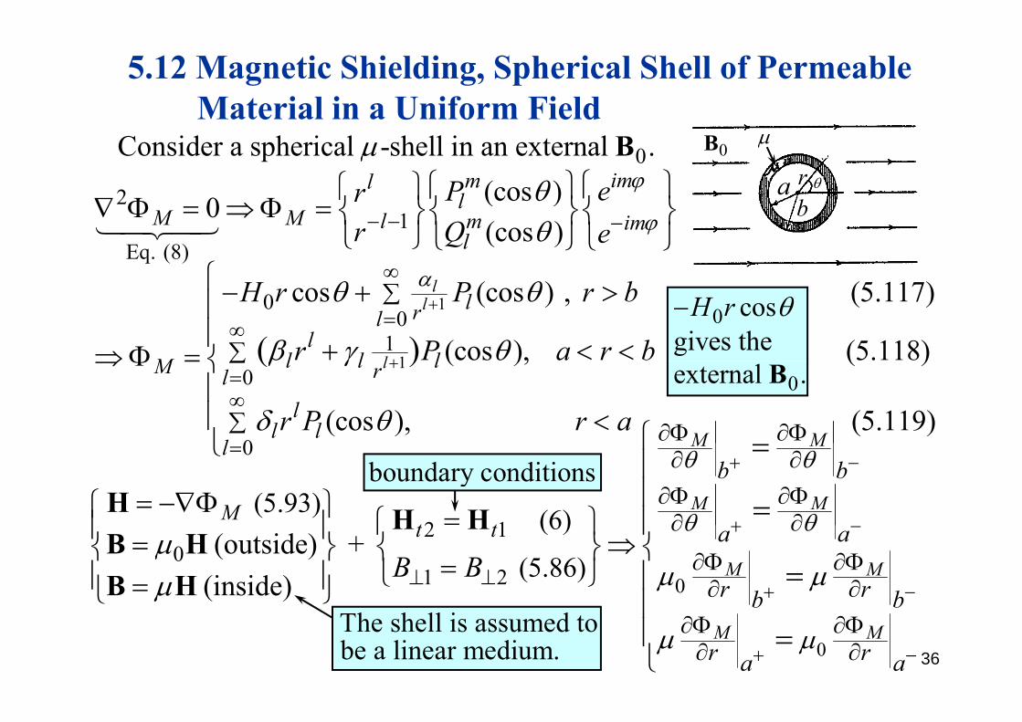
5.12 Magnetic Shielding, Spherical Shell of Permeable Material in a Uniform Field
0
2
Consider a spherical -shell in an external .(cos ) imml
l ePr
B
a
0 B
r
Material in a Uniform Field
21
Eq. (8)
(cos )0(cos )
lM M l m im
l
ePrr Q e
b
100
cos (cos ) , (5.117)
(
ll lrl
M
H r P r b
11 (cos ), (5.118))l
ll l lr P a r b
0 cosgives the
H r
(M 10
0
( ), ( )
(cos ), (5.119)
)ll l lrll
l ll
r P r a
M M
0external .B
0l
2 1(5.93) (6)
M M
M MMt t
b b
H H H
boundary conditions
0
2 10
1 2
(6)
(5.86)
(outside) +
(inside)M M
t t a a
r rb bB B
H HB H B H
0M M
b b
r ra a
The shell is assumed to be a linear medium. 36

5.12 Magnetic Shielding, Spherical Shell of Permeable Material in a Uniform Field (continued)
Boundary conditions result in solutions for the coefficients:
3 330 0
(2 1)( 1)( )
0 if 1
l l l l
b a
l
H b H
30 0
1 0 03 230 0 0
(2 1)( 2) 2 ( 1)
ab
H b H
9
(5.121) &
9
0
33
001 0 03 2
30 0 0
9
(2 1)( 2) 2 ( 1)
9 (5.122)2 1( )
ab
ab
H H
0 0 as , implying that materials tend to "absorb" -field lines and
in
bB
B0 field+ dipoleout B B
materials tend to absorb field lines andthereby prov
B
3 60
ide the shielding effect. High-materials can have / as high as 10 10 .
0
0 0
g When , reduces to everywhere, i.e. a static megnetic field penetrates into the
B B
: uniform fieldBshell as if there were no shell present (even if theshell is made of good conductor, such as copper). 0
: uniform field( 1/ if )
inB
37

5.15 Faraday’s Law of InductionThe Biot-Savart (or Ampere's) law relates the magnetic field to The Biot Savart (or Ampere s) law relates the magnetic field to
electrical . Faraday then discovered thattime-varying magnetic flux through an electrical
experimancircuit c
tallould
curren
yt
induce an electric field around the circuit. This not only providedthe first link between electric and magnetic fields, but also led to a
h i t t th fi ld i ti i fi ldE B
( )B
loop C
new mechanism to generate the -field, i.e. a time-varying -field.
E B Referring to the figure, let loop
be an electrical circuit (as in Faraday'sC
dda
n( , ) tB xbe an electrical circuit (as in Faradays
original experiment) or any closed path in space (a generalization of the originalp ( g gobservation with immense consequences). Faraday's law states
: an arbitrary surface , (5.141) bounded by loop h i h l i fi ld i h f i hi h i
cSdas t C
d d
d
B n
E
E
where is the electric field at in the frame in which is atrest, and is th
d dEB
e magnetic induction in the lab frame. 38

loop CR i (5 141)
5.15 Faraday’s Law of Induction (continued)
d n( , ) tB x
loop C Rewrite (5.141):
(5.141) c das td B nE da Assume loop is at rest in the lab
frame, then (electric field in the
tC
E E lab frame) and (5.141) becomes
integral form of Faraday's law (9) c das td B nE ( )
where both and are lab-frame quantities.
(9) b itt (b St k ' th
c s t
dE B
EE ) d (9) can be written (by Stokes's theorem: c d EE )
dasda das s t
nBE n n
Thus,
differential form of Faraday's law) (5.143)
t
tBE y ) ( )t
39
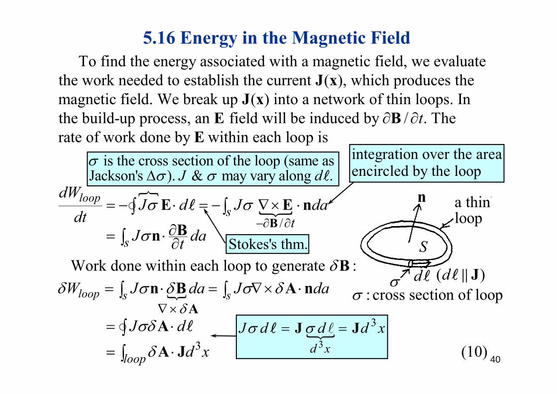
To find the energy associated with a magnetic field we evaluate5.16 Energy in the Magnetic Field
To find the energy associated with a magnetic field, we evaluate the work needed to establish the current ( ), which produces the magnetic field. We break up ( ) into a network of thin loops. I
J xJ x n
the build-up process, an field will be induced by / . Therate of work done by within each loop is
tE BE
integration over the area
n hi
loopdW
is the cross section of the loop (same as Jackson's ). & may vary along . J d
integration over the areaencircled by the loop
n
S
a thin loop
/
loops
st
dWJ d J da
dtJ dat
BE E n
Bn
St k ' th
S
d ( )d J Work done within each loop to
s tgenerate :
W J da J daB
n B A n
Stokes's thm.
: cross section of loop
loop s sW J da J da
J dA
n B A n
A 3J d d d x J J3 (10)
loop
Jd xA J
3d xJ d d d x J J
40

3 As shown in [(10)], the work done withinlooploopW d x A J5.16 Energy in the Magnetic Field (continued)
each loop is an integral over the volume of the loop. Thus, an inte-gration over all space gives the total work done to
pp
generate :B
3 3( ) (5 144)W d x d x A J A H
Assume the rate of build-up 0 obeys the static law .Otherwise, the static law breaks down and there will be radiation loss.
H H J
3 3 ( ) (5.144) ( ) ( )
W d x d xd x d x
A J A HH A H A For this integral
to vanish the3 3
( ) 012 ( )
dsd x d x
B H A a
H B H B to vanish, the
volume of integ- ration must be .
Total woB ti f thi i
rk done to bring the field up from 0 to the final value :
BAssume linear medium: or B H B μ H
3 By conservation of energy, this isthe total magnetic field energy.
12
12 (5.148)
[field energy den
)
si
(W d x
w
B
B
H
H ty] (11)2 [ gy1 1 12 2 2
y] ( ) : ( ) ( ) ( ) j j j j
j j jNote w H B H B H B
41

5.17 Energy and Self- and Mutual InductancesAssume linear relation between J and A
3 312 ( ) (5.144) W d x d x A JJ A
for nonpermeable(μ0) medium
Assume linear relation between J and A
0
3
3 3
12 (5.149)
( ) (W d x
A JJ x J )
x
0 3( )( ) (5.32)4 | | d x
J xA x x x
f N t0 3 3 ( ) ( 8 d x d x
J x J
3 3 21
(5.153)
( ) ( )
| |)
N N N N Ni j
J x J x
xxx
for N current-carrying circuits
0 3 3 2
1 1 1 112
( ) ( ) , (5.152)8 | |
where
N N N N Ni j i i ij i j
i j i i j i
i ji j
d x d x L I M I I
J x J x
x xself-inductance for a thin wire
0
where
4ii
L I
02
3 3 ( ) ( ) (5.154)4| | | |i iC Ci i C Ci ii ii i i i
i id dd x d x
J x J xx x x x
self-inductance for a thin wire
i
0 03 3
| | | |
( ) ( ) (5.155)4 4| | | |i jC Ci j C Cij i j
i i i i
i jj i j i j
i ji
d dM d x d xI I
J x J x
x x x x
4 4| | | | i jC Ci j C Cj jj i j i jiI I x x x x
mutual inductance (Mij = Mji) for thin wires 42

0 3( )( ) (5 32)d J xA
5.17 Energy and Self- and Mutual Inductances (continued)
0 3( ) ( ) (5.32)4 | |Vector potential at circuit due to current in circuit :
d x
i j
J xA x x x
0 3( ) ( ) 4 | |jC
jij i ji j
d x
J x
x x xA (12)
31 From (12) and (5.155), we obtain ( ) ( )
Assume flows along wire of negligible cross sectioniCij ij i i ii jI IM d x
d da
A x J x
J 3
Assume flows along wire of negligible cross section
( )i i
d da
J dadd x
J
J x
ijiI d
B magnetic flux from circuit j
passing through circuit i
1 1 1 (5.156)( )Ci i
ij
ij ij ijijsj j jI I IM d da F
B
A A
n
Th “ ” i i li th t th i d d t d t d i t i
jij ij ij Id dF Mdt dt ij: induced voltage in circuit i due
to current variation in circuit j.
The “–” sign implies that the induced ij tends to drive a current in circuit i to inhibit the flux change caused by circuit j (Lenz’s law). 43

Homework of Chap. 5
Problems: 1, 3, 6, 11, 13, , , , , ,
18, 19, 20, 22, 30
44