chapter 5 property investment valuation - wiley- · pdf fileproperty investment valuation 249...
TRANSCRIPT

5.1 Introduction
Around half of all commercial and industrial properties in the UK are held
as investments, where the ownership interest is separate from the occupation
interest. The landlord leases the property to an occupying tenant or ten-
ants. Investors in UK commercial property include large financial institutions
such as pension funds and insurance companies (28%), overseas investors
(15%), UK listed property companies (14%), UK private property compa-
nies (15%), limited partnerships, landed estates, charities, trusts, unitised
and pooled funds and private investors (23%) (IPF, 2005). The majority of
commercial property investments can be placed in one of three principal sec-
tors: retail (shopping centres, retail warehouses, standard shops, supermar-
kets and department stores), offices (standard offices and business parks);
and industrial (standard industrial estates and distribution warehousing).
Investment market sub-sectors are often defined using a combination of this
sector classification and their location, ‘City of London offices’ or ‘south
west high street retail’, for example. There are also several smaller sectors
of the property market that attract investment interest such as leisure parks,
restaurants, pubs and hotels.
Property that is typically held as an investment is valued with this purpose
in mind; the valuer will capitalise the rental income produced by the property
at an appropriate investment yield using the investment method of valuation,
as we saw in Chapter 3. The underlying principle is to discount net economic
benefits from an investment over its predicted life at a specified rate of return
or discount rate. Chapter 2 described discounting as the process of finding the
present value (PV) of expected net benefits that may be in the form of a regu-
lar income, a future capital reversion or a combination of the two (Havard,
2000). The all-risks yield (ARY) technique described in Chapter 3 is based
on the assumption that there is a relationship between the price paid (capi-
tal value) and the annual return (net rental income). This chapter develops
this notion more explicitly and describes a technique for valuing a property
Chapter 5Property Investment Valuation
Wyattp-05.indd 248Wyattp-05.indd 248 8/18/2007 12:10:21 PM8/18/2007 12:10:21 PM

Property Investment Valuation 249
Ch
apte
r 5
investment that involves more direct recourse to the underlying cash-flow
characteristics of the investment. Before that, though, a history lesson.
Up until the 1960s landlords who wished to lease commercial properties
typically did so using long leases with no rent reviews. Investment in these
commercial premises was regarded as low risk. Consequently the required
(or target) rate of return was closely linked to similar low-risk investments
such as gilts. Conventionally a premium of around 1–2% was added to the
redemption yield on long-dated gilts to account for property market risk.
Long-dated gilts were used as a benchmark because property was regarded
as a long-term investment. Valuation of property investments involved ana-
lysing comparable evidence to determine the appropriate yield which was,
in fact, mathematically and logically equivalent to the target rate of return
(TRR) (Baum and Crosby, 1995). No adjustment was made to either the
yield or the rent to reflect income or capital growth because there was none.
A typical investment valuation prior to the 1960s is shown below.
Market rent (MR)(£) 10 000Years’ purchase (YP) perpetuity @ 10%a 10Valuation (£) £100 000aInvestor’s target return and therefore comparable with other investments.
After the 1960s, and a period of limited supply of new commercial and indus-
trial property and restrictive macroeconomic policy, commercial property rents
increased significantly and landlords introduced rent reviews into shortening
leases so that they did not miss out on rising rents. Property became a growth
investment, more like equities than fixed interest bond investments, albeit with
a peculiar income pattern that goes up (usually) every 5 years (Havard, 2000).
Investors were prepared to accept a lower return at the start of the investment
term in expectation of higher returns later on. Property investment valuation
techniques handled this change not by explicitly forecasting rental growth but by
capitalising the current rent at an ARY (derived from comparable evidence) that
is lower than the TRR because it implies future rental income and capital growth
expectations. The gap between the two represented the expected or implied rental
growth hidden in the valuation – directly analogous to the concept of a reverse
yield gap between equities and bonds (Baum and Crosby, 1995). Consequently,
the assumed static cash-flow is not the expected cash-flow, the yield is not the
target rate and is not comparable to target or discount rates used to capitalise or
value income from other investments. A typical investment valuation after the
1960s is shown below.
MR (£) 10 000YP perpetuity @ 8%a 12.5Valuation (£) £125 000
aGrowth implicit ARY, not the target rate and therefore not comparable with other investments.
From Chapter 3 we know that the ARY investment valuation technique
relies on comparison to justify adjustments to initial yields obtained from
Wyattp-05.indd 249Wyattp-05.indd 249 8/18/2007 12:10:21 PM8/18/2007 12:10:21 PM

250 Property Valuation
Ch
apter 5
comparable investment transactions. These adjustments account for all
factors that influence investment value except those that can be handled
by altering the rent such as regular/annual management and maintenance
expenditure. The most important investment characteristics that need to be
reflected in the ARY are income and capital risk and growth potential, but
influencing these characteristics are a multitude of economic and property-
specific factors including macroeconomic conditions, property market and
subsector activity, the financial standing of individual tenants, property depre-
ciation and changes in planning, taxation, landlord and tenant legislation.
The ARY has to implicitly quantify these factors and the all-encompassing
nature of the ARY means that capital value is very sensitive to small adjust-
ments. In essence, a single divisor (ARY) or multiplier (YP) conceals many of
the assumptions regarding choice of TRR (which includes risk) and income
and capital growth expectations.
Nevertheless, the ARY approach is practical and appropriate where there
is a plentiful supply of comparable market transactions providing evidence
of yields, rents and capital values. But there are circumstances when it is par-
ticularly difficult to use the ARY technique to value a property investment.
Problems arise when, first, comparable evidence is scarce, either because
market activity is slow or the property is infrequently traded, and second,
where there is greater variability in investments, meaning more variables
must be accounted for in the ARY. Regarding this latter point, we saw in
Chapter 4 how flexi-lease terms are creating greater diversity in property
investment cash-flows, often with gaps in rental income. But, in addition to
that, non-prime properties are generally more variable in terms of location,
physical quality, condition or covenant and are therefore more risky. And
problems arise where the property is more complicated than a simple rack-
rented investment: the ARY technique is inappropriate for valuing property
that is over-rented, let on short leases or produces varying rental income
streams from multiple tenants. It can be especially difficult to quantify all of
these factors in an ARY when comparable evidence is scarce.
Harvard (2000) notes that increasing diversity in the property investment
market has undermined the ARY valuation technique because it relies heav-
ily on comparison between relatively homogeneous investment assets and
simple adjustments to comparable evidence. As a result, property investment
valuation techniques have emerged that focus more explicitly on the TRR
that an investor requires, the expected flow of income, expenditure and
capital growth that might be expected from an investment. The discounted
cash-flow (DCF) technique uses an established financial modelling technique
that allows comparison between property and other forms of investment.
Where information is scarce, or when an unusual property is being val-
ued, the DCF technique assists in the consideration of income and capital
growth, depreciation, timing of income receipts and expenditure payments
and the TRR. Indeed, International Valuation Standards now include guid-
ance on the use of DCF analysis for valuation in GN9 – Discounted Cash Flow Analysis for Market and Non-market Based Valuations (IVSC, 2005).
The guidance describes how DCF analysis involves the projection of a cash-
Wyattp-05.indd 250Wyattp-05.indd 250 8/18/2007 12:10:21 PM8/18/2007 12:10:21 PM

Property Investment Valuation 251
Ch
apte
r 5
flow for an operational or development property. This projected cash-flow is
discounted at an appropriate market-derived discount rate to establish PV. In
the case of standing investment properties, the cash-flow is typically a series
of periodic net rental incomes (gross income less expenditure) along with an
estimate of reversion value anticipated at end of the projection period. In the
case of development properties’ estimates of capital outlay, development costs
and anticipated sales income produce a net cash-flow that is discounted over
the projected development and marketing periods (cash-flows from property
development will be covered in the Chapter 6). The guidance note discusses the
structure and components of DCF models and the reporting requirements for
valuations based on DCF analysis.
5.2 A DCF valuation model
The academic case for valuing property investments by capitalising a DCF at
a TRR rather than capitalising an initial income estimate at an ARY derived
from comparable evidence began in the late 1960s and continues to this day.
Appendix 5A (see Appendix 5A at www.blackwellpublishing.com/wyatt)
lists references to papers that make this case in detail, culminating in the
seminal UK text book in this field by Baum and Crosby (1995). But what-
ever valuation technique is employed, it must reflect the behaviour of market
participants. Recourse to comparable evidence (which is generated by mar-
ket transactions) whenever possible and the adoption of pricing models that
are used by market participants will undoubtedly be the most reliable and
consistent way of estimating market price.
The ARY technique relies on analysis of prices and rents achieved on recent
comparable transactions to estimate an ARY for the subject property. The
growth-implicit ARY is then used to capitalise an initial estimate of the cash
flow. The DCF technique capitalises or, in the language of investment math-
ematics, discounts the actual or estimated cash-flow at the investor’s TRR.
The DCF technique requires explicit assumptions, based on evidence, to be
made regarding several factors but most importantly the TRR (which should
cover the opportunity cost of investment capital plus perceived risk) and
expected rental income growth. When a valuer capitalises an initial rent at
an ARY of, say, 8% it is done so in the knowledge that the investor is antici-
pating a return in excess of 8% over the period of ownership as the expecta-
tion is that rental income and perhaps capital value will increase. Essentially,
the DCF technique removes the growth element from the ARY and puts it in
the cash-flow. As a result, it re-establishes the relationship between the TRR
required from a property investment and those required from other invest-
ments, as was the case before the 1960s when rental growth was negligible.
Instead of simply capitalising the current income (actual or estimated) at an
ARY, the expected cash-flow, projected over a certain period of time at a
rental growth rate, is discounted at a TRR.
Of course, as we shall see, the DCF technique is not a panacea and several
criticisms can be levelled at it. The selection of the discount rate or TRR is
Wyattp-05.indd 251Wyattp-05.indd 251 8/18/2007 12:10:22 PM8/18/2007 12:10:22 PM

252 Property Valuation
Ch
apter 5
subjective and the Appraisal Institute (2001) argues that it is difficult to find
market-supported estimates for the key variables in the cash-flow. It might
be necessary to estimate current market rent (MR) and expected changes
over the next few years. It might also be necessary to try and predict what
will happen when the tenant has an option to break or when the lease needs
renewing. The variation in possible lease incentives that might be offered,
length of possible voids and expenditure that might be incurred is consider-
able. Moreover, because the DCF technique separates the value significant
factors as distinct inputs into the cash-flow and even separates the discount
rate into a TRR and an exit yield, the risk of double-counting the effect on
value of these factors is high.
5.2.1 Constructing a DCF valuation model
The relationship between the growth-implicit ARY and the growth-explicit
DCF techniques can be represented by a simple equation:
y r g= - [5.1]
where y is the ARY, r is the investor’s target return and g is the annual rental
growth rate.
The left side of the equation represents the growth-implicit ARY technique
and the right side represents a growth-explicit DCF technique. The DCF
technique separates the ARY into two elements; a rental income growth rate
and a TRR; in other words, the ARY implies the rental growth that the inves-
tor expects in order to achieve the TRR. An investor accepting a relatively
low initial yield from a property investment when higher yields might be
available from fixed interest investments implies an expectation of future
income growth. For example, an investor with a target rate of 15% who
purchases a property investment for a price that reflects an initial yield of
10% would require a 5% annual growth to achieve the target rate. This sim-
ple relationship is made more complex in the UK property market because
income from property investments (in the form of rent) is normally reviewed
every 5 years. This means that a slightly higher annual growth rate will be
required to meet the investor’s annual TRR. Provided the growth rate, target
return and rent review period in the DCF approach are mathematically con-
sistent with the yield adopted in the ARY approach, the valuation will be the
same. The following explains why.
Starting with the ARY approach, the present (capital) value, V of an income
stream from a rack-rented freehold property investment is the pv PV £1 pa or YP
(see Equation 2.18 in Chapter 2) multiplied by the annual income or MR:
V
y
n
=(1+Y) )
MR1−(1
[5.2]
where y is the growth-implicit ARY and n is the number of years for which
the rent is received. If the rent is receivable in perpetuity, that is, freehold
Wyattp-05.indd 252Wyattp-05.indd 252 8/18/2007 12:10:22 PM8/18/2007 12:10:22 PM

Property Investment Valuation 253
Ch
apte
r 5
property investment, the above formula simplifies to Equation 2.23 from
Chapter 2:
V
y=
MR
In other words, the PV is equivalent to a constant annual income capital-
ised at (divided by) the ARY. In the case of the DCF technique, the income
stream is discounted at the investor’s TRR, r, rather than the ARY. So the PV
of a rack-rented freehold property investment which consists of a constant
(i.e. non-growth) annual MR receivable in perpetuity annually in arrears can
be expressed as follows:
V
r= MR
[5.3]
But because the DCF technique is explicit about income growth we now
need to introduce rental income growth, g, into this valuation model. Let us
assume rent is receivable in perpetuity and there are annual rent reviews at
which the rent is increased at the estimated long-term average annual rental
growth rate, g. Assuming r, g, rental growth can be incorporated as follows:
V
r g=
-MR
[5.4]
But for most property investments rent does not grow each year. If non-
annual rental growth is now introduced, the following equation represents a
freehold property recently let at MR in perpetuity with 3 year reviews:
V = + + + +MR + + +�+•(1+ r) (1+ r)2 (1+ r)3 (1+ r)4 (1+ r)5 (1+ r)6 (1+ r)7
MR (1+g) MR (1+g) MR (1+g)3 MR (1+g)3 MR (1+g)3 MR (1+g)6
The above expression (which is a geometric progression) simplifies to:
Vr - r
= ((1+g) −1) ((1+ r −1)) ÈÎ
˘˚
MR3 3
[5.5]
Rearranging Equation 2.23 we can show that MR/V = y and, substituting
these variables into Equation 5.5, the relationship between the ARY and
DCF techniques can be shown by:
y r r= -
ÊËÁ
ˆ¯
p(1+ g) -1p(1+ r ) -1
[5.6]
This is the property yield equation derived by Fraser (1993) and based on
a rack-rented freehold property investment. It shows that y is determined
by the investor’s TRR, r, the annual rental growth rate, g, and the number
of years between each rent review (the rent review period), p. This equation
is the same as Equation 5.1 except that the annual rental growth rate g has
Wyattp-05.indd 253Wyattp-05.indd 253 8/18/2007 12:10:22 PM8/18/2007 12:10:22 PM

254 Property Valuation
Ch
apter 5
been increased to compensate for the fact that rental growth is not actually
received until each non-annual rent review.
If the property to be valued is rack-rented and the rent and review period
are known, then, applying the ARY technique, the valuer only has one vari-
able, ARY, to predict in order to value the property. If sufficient evidence
is available this is straightforward. With the DCF technique there are two
unknowns: the investor’s TRR and the growth rate. To predict the growth
rate it is necessary to compare yields on recently let comparable freehold
properties with an estimate of the investor’s target return for those proper-
ties. Armed with this information and rearranging Equation 5.6 an average
annual growth rate can be implied as follows:
g
r
p
=Ê
ËÁ
ˆ
¯˜ -1
1
(r-y)(1+ r)p + y
[5.7]
Where g is the annual rental growth expectation, y is the yield obtainable from
comparable properties, p is the period between rent reviews in years and r is the estimated target return for properties of this type. The complexity of this
formula is due to the rent review periods being greater than 1 year. If reviews
were annual, the growth rate would be the target rate minus the initial yield
on a rack-rented freehold property (g = r – y). For example, if an investor
accepts an initial yield of 8% but requires an overall return of 12%, then the
income must grow by 4% over the year. But with 5-year rent reviews
g
g
=-( )Ê
ËÁ
ˆ
¯˜ -
=
0 12 0 080 12
1
4 63
1 5. .
.
. %
p
(1+ 0.12) + 0.08)
So an investor accepting an initial yield of 8% would require 4.63% per
annum growth in the income, on average (compounded at each review) to
achieve the target return. Figure 5.1 illustrates this.
Ren
t (£)
If price paid at this point produces an initial yield of 8% then the stepped rent would have to grow at an average rate of 4.63% per annum to achieve a target rate of 12% per annum
Rate to which the stepped rent must grow at each review to equate to an annual growth rate of 4% per annum
Growth in actualrent paid (stepped)
Marketrent
0 5 10
Time (years)
15 20
Figure 5.1 Rental growth. The fi gure assumes rent received in perpetuity (The fi gure assumes rent received in perpetuity).
Wyattp-05.indd 254Wyattp-05.indd 254 8/18/2007 12:10:23 PM8/18/2007 12:10:23 PM

Property Investment Valuation 255
Ch
apte
r 5
Equation 5.7 is often referred to as the implied rental growth rate formula.
The higher the client’s target rate relative to the market-derived ARY, the
better the investment must perform over the holding period to achieve the
desired level of return. Comparable evidence can be used to ascertain the
implied growth rate necessary to reconcile an ARY valuation with a DCF
valuation (Crosby, 1990). The implied growth rate formula is constructed
on assumption that property is rack-rented. g represents the market’s expec-
tations of future growth and is an average growth rate. In fact it is a dis-
counted growth rate into perpetuity so g is influenced by expectations in the
near future more than ones further away (Fraser, 1993). As an alternative
it is possible to derive an explicit growth rate from direct analysis of rental
growth rates prevalent in various market sectors, regions and towns. Some
argue that the assumption of a stable and constant growth rate is simplistic
but it can be taken to be an adequate reflection of the decision-making pro-
cess of most investors. Before looking at the practical application of the DCF
technique the next section will look at the input variables in more detail.
5.2.2 Key variables in the DCF valuation model
The key, value significant, variables in the DCF technique are the rent, rental
growth rate, the TRR and the exit yield. Other variables include regular and
periodic expenses, transaction fees and taxes, but these are determined in rela-
tion to the key variables and their estimation is relatively straightforward.
The rent must be net of any regular or periodic expenditure and the esti-
mation of MR is undertaken in the same way as for the ARY technique
described in Chapter 3. Rental growth can be separated into two compo-
nents; growth in line with inflation and real growth in excess of inflation.
Depreciation is the rate at which the MR of an existing property falls away
from the MR of a property that is comparable in all respects except that
it is (hypothetically) permanently new. The causes of depreciation, namely
deterioration and obsolescence, will be discussed in Chapter 6. So, assuming
constant rental growth, an annual rate of rental growth must be net of an
average annual rate of depreciation. As these two components are interact-
ing growth rates their mathematical relationship with is (Fraser, 1993):
g g d dg= - -m m [5.8]
Where g is the average annual rental growth rate of actual property, gm is
the average annual rental growth rate of permanently new property and d
is the average annual rate of depreciation. As dgm is usually very small the
equation can be simplified to:
g g dm= - [5.9]
A valuer may buy in or undertake research aimed at forecasting explicit
rental growth rates and movements in capital values. Simple models might
take the form of an historic time series of rents and capital values from
which a moving average or exponentially smoothed set of values for future
Wyattp-05.indd 255Wyattp-05.indd 255 8/18/2007 12:10:25 PM8/18/2007 12:10:25 PM

256 Property Valuation
Ch
apter 5
years might be predicted. More complex regression-based models will pro-
duce equations which identify independent variables such as GDP or other
output measures, expenditure, employment, stock, vacancy, absorption and
development pipeline and measure their effect on a dependent variable such
as rental growth or yield (Baum, 2000). The Investment Property Databank
(IPD) publishes figures for rental value growth for the properties in its data-
bank (which, it should be remembered, are prime institutional investments
in the main). Figures are published by sector, segment and region and within
these broad groupings it is possible to examine the rental growth of various
sectors of the property investment market and their broad location. Using
these figures it is possible to get a feel for the rental growth rates of prime
investment grade property. Table 5.1 shows how badly office investments
in the City of London have performed recently, especially in comparison to
Mid Town and West End offices and only mid-sized office space did not pro-
duce negative rental value growth in 2004. The annualised returns between
1999 and 2004 and 1994 and 2004 show that, over the longer term, things
looked a little healthier but still lagged performance to the west of the City.
A similar analysis of rental growth for single-let standard shop units, shop-
ping centres and retail warehousing reveals significant differences in perfor-
mance, as can be seen from Table 5.2.
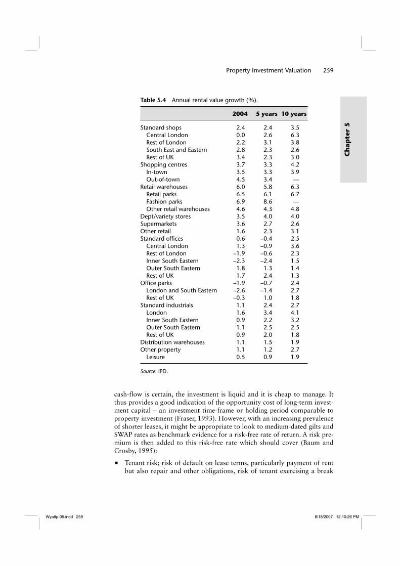
A more detailed regional and sector breakdown of rental value growth
can be performed using IPD data and two examples are shown in Tables 5.3
and 5.4.
This sort of market intelligence, although not at the individual property
level, paints a very useful picture of rental growth performance across the
main investment sectors and locations in the UK and allows an implied rental
growth rate to be verified against growth rates achieved in the market. As the
tables above demonstrate, a great deal of rental growth information about
prime investment property can be obtained from IPD and this information
can be used to derive explicit rental growth rates depending on property type
and location. It must be remembered, though, that rents can be volatile in the
short-term and very little is known about depreciation rates and their effect
Table 5.1 Annual rental value growth (%).
Floor area (m2)
Offi ce investments in 0–1000 1001–2500 2501–5000 5001–10 000 10 001+
City 2004 –2.0 –3.4 0.0 –2.5 –1.4 1999–2004 –0.9 –1.6 –2.2 –1.8 –3.2 1994–2004 3.5 3.2 3.2 2.7 1.8Midtown/West End 2004 1.0 4.0 3.7 2.6 5.1 1999–2004 –0.7 0.2 0.6 0.2 1.6 1994–2004 5.0 5.3 4.8 5.2 4.3
Source: IPD.
Wyattp-05.indd 256Wyattp-05.indd 256 8/18/2007 12:10:25 PM8/18/2007 12:10:25 PM

Property Investment Valuation 257
Ch
apte
r 5
on rental growth prospects in the long-term. As an alternative, therefore, a
long-term average expected ‘market’ rental growth rate can be implied from
the relationship between the ARY derived from comparable evidence and
the target rate on rack-rented freehold property investments. The way that
this implicit growth rate can be calculated was shown in Section 5.2.1. The
growth rate should be indicative of rental growth on properties regardless
of whether they are rack-rented or reversionary freeholds or leaseholds (but
with due care exercised in the case of geared profit rents). Also, if attempting
to derive an implied growth rate from a reversionary comparable transac-
tion it is important to bear in mind what Brown and Matysiak (2000) say in
Section 5.2.3 below.
The TRR (also referred to as the equated yield or discount rate because
it is the rate at which cash-flows are discounted to PV) should adequately
compensate an investor for the opportunity cost of capital plus the risk that
the investor expects to be exposed to. It is therefore a function of a risk-free
rate of return and a risk premium: a higher risk premium (and thus higher
target rate) would be used to discount the future cash-flow of a more risky
property investment and cause its PV to reduce accordingly. It is difficult to
obtain evidence of the target rate from the market but the base-line is the
return from a risk-free investment. The closest available proxy for the risk-
free rate is the gross redemption yield on long-dated fixed interest gilts; the
Table 5.2 Annual rental value growth (%).
2004 1994–2004 1999–2004
Single-let standard shops by fl oor area (m2) 0–250 2.0 2.2 3.1 251–500 2.6 1.9 3.1 501–1000 3.4 2.4 3.4 1001–2000 3.0 2.5 3.8 2001+ 2.3 2.7 5.2 All single-let standard shops 2.9 2.4 3.6Shopping centres by fl oor area (m2) 0–7000 3.3 3.4 3.6 7001–14,000 2.5 3.0 2.7 14,001–25,000 2.9 3.7 3.8 25,001–50,000 3.6 3.1 4.2 50,001+ 4.7 3.4 6.0 All shopping centres 3.7 3.3 4.2Retail warehouses by fl oor area (m2) 0–2500 4.0 4.3 4.7 2501–5000 4.3 4.1 4.4 5001–10 000 5.4 5.3 5.7 10 001–15 000 6.4 6.6 7.4 15 001+ 7.9 7.2 8.3 All retail warehouses 6.0 5.8 6.3
Source: IPD.
Wyattp-05.indd 257Wyattp-05.indd 257 8/18/2007 12:10:25 PM8/18/2007 12:10:25 PM

258 Property Valuation
Ch
apter 5
Tab
le 5
.3
Ann
ual r
enta
l val
ue g
row
th (
%).
City/Mid- Town
West End
C. London Fringe
Rest of London
South East
South West
Eastern
East Midlands
West Midlands
North West
Yorks & Humber
North East
Scotland
Wales
Reta
ils
2004
0.7
0.5
3.8
4.9
4.9
4.9
3.5
3.7
3.9
5.2
5.0
3.0
4.4
19
99–2
004
2.4
2.7
4.1
4.2
3.4
4.0
3.7
4.2
3.6
3.8
3.6
2.9
3.6
19
94–2
004
5.7
6.4
4.4
4.2
3.6
4.8
4.4
4.4
4.3
3.9
4.8
4.1
3.8
Stan
dard
ret
ails
20
040.
60.
02.
52.
85.
32.
83.
32.
32.
65.
63.
21.
32.
6
1999
–200
42.
22.
73.
22.
42.
92.
42.
42.
32.
33.
42.
61.
02.
3
1994
–200
45.
96.
33.
72.
62.
62.
43.
42.
43.
33.
33.
73.
53.
0Re
tail
war
ehou
ses
Lond
on
2004
4.4
7.4
6.8
6.9
5.8
5.4
5.9
6.1
5.6
6.1
5.4
19
99–2
004
5.8
6.6
6.1
6.6
6.2
5.4
6.3
4.5
5.2
4.9
4.1
19
94–2
004
6.1
6.1
6.7
6.5
7.4
6.8
6.5
6.1
6.7
5.2
5.4
Offi
ces
Out
erLo
ndon
20
04–1
.70.
44.
6–2
.8–2
.11.
20.
1–0
.81.
82.
81.
02.
6–0
.11.
7
1999
–200
4–2
.4–0
.70.
6–0
.8–2
.22.
71.
00.
62.
02.
71.
72.
21.
80.
8
1994
–200
42.
34.
05.
02.
31.
31.
02.
50.
91.
42.
00.
51.
51.
50.
3In
dust
rials
Lond
on
2004
1.5
1.0
1.5
1.6
0.5
0.8
0.3
2.2
3.1
0.5
–0.6
19
99–2
004
3.3
2.1
1.8
2.6
1.3
1.6
2.1
1.7
1.6
1.8
2.5
19
94–2
004
4.1
3.
11.
72.
31.
61.
71.
61.
01.
51.
52.
4
Sour
ce: I
PD.
Wyattp-05.indd 258Wyattp-05.indd 258 8/18/2007 12:10:26 PM8/18/2007 12:10:26 PM
Property Investment Valuation 259
Ch
apte
r 5
cash-flow is certain, the investment is liquid and it is cheap to manage. It
thus provides a good indication of the opportunity cost of long-term invest-
ment capital – an investment time-frame or holding period comparable to
property investment (Fraser, 1993). However, with an increasing prevalence
of shorter leases, it might be appropriate to look to medium-dated gilts and
SWAP rates as benchmark evidence for a risk-free rate of return. A risk pre-
mium is then added to this risk-free rate which should cover (Baum and
Crosby, 1995):
Tenant risk; risk of default on lease terms, particularly payment of rent
but also repair and other obligations, risk of tenant exercising a break
Table 5.4 Annual rental value growth (%).
2004 5 years 10 years
Standard shops 2.4 2.4 3.5 Central London 0.0 2.6 6.3 Rest of London 2.2 3.1 3.8 South East and Eastern 2.8 2.3 2.6 Rest of UK 3.4 2.3 3.0Shopping centres 3.7 3.3 4.2 In-town 3.5 3.3 3.9 Out-of-town 4.5 3.4 —Retail warehouses 6.0 5.8 6.3 Retail parks 6.5 6.1 6.7 Fashion parks 6.9 8.6 — Other retail warehouses 4.6 4.3 4.8Dept/variety stores 3.5 4.0 4.0Supermarkets 3.6 2.7 2.6Other retail 1.6 2.3 3.1Standard offi ces 0.6 –0.4 2.5 Central London 1.3 –0.9 3.6 Rest of London –1.9 –0.6 2.3 Inner South Eastern –2.3 –2.4 1.5 Outer South Eastern 1.8 1.3 1.4 Rest of UK 1.7 2.4 1.3Offi ce parks –1.9 –0.7 2.4 London and South Eastern –2.6 –1.4 2.7 Rest of UK –0.3 1.0 1.8Standard industrials 1.1 2.4 2.7 London 1.6 3.4 4.1 Inner South Eastern 0.9 2.2 3.2 Outer South Eastern 1.1 2.5 2.5 Rest of UK 0.9 2.0 1.8Distribution warehouses 1.1 1.5 1.9Other property 1.1 1.2 2.7 Leisure 0.5 0.9 1.9
Source: IPD.
Wyattp-05.indd 259Wyattp-05.indd 259 8/18/2007 12:10:26 PM8/18/2007 12:10:26 PM

260 Property Valuation
Ch
apter 5
option or not renewing lease (higher risk if the lease is short). The level
of tenant risk will depend to an extent on the type of tenant; a public sec-
tor organisation may be considered less likely to default than a fledgling
private sector company. Physical property risk; management costs (e.g. rent collection, rent
reviews and lease renewal) and depreciation. This type of risk is less
acute in the case of prime retail premises because land value is a high
proportion of total value, but the reverse is true for, say, small industrial
units. A certain amount of physical property risk can be passed on to the
tenant via lease terms. Property market risk; illiquidity caused by high transaction costs, com-
plexity of arranging finance and accentuated by the large lot size of prop-
erty investments. Macroeconomic risk; fluctuating interest rate, inflation, GDP, and so on,
all affect occupier and investment markets in terms of rental and capital
values and potential for letting voids. Planning risk; in the main, this refers to planning policy and development
control. For example, Sunday trading, presumption against out-of-town
retailing, promotion of mixed-use, city centre developments on previ-
ously developed land.
Baum and Crosby (1995) point out that, for valuation, it is not feasible to
quantify all of these components of risk as this would need to be done for
each comparable – this sort of thing is more appropriate in property invest-
ment appraisal (see Chapter 7). Instead, the valuer subjectively chooses and
adjusts a target rate not at the individual property level but by grouping
various property investments and examining the risk characteristics of each.
By far the most frequently encountered investment type is a rack-rented free-
hold. Regular rent reviews mean that this is an equity-type investment that
benefits from income and capital growth just as equities do, albeit with less
frequent income growth participation. Whereas the return from an invest-
ment in company shares relies on the continued existence and profitability
of that company, a property investment will remain even if the occupying
company fails. Unlike share dividends, rent is a contractual obligation paid
quarterly in advance and is a priority payment in the event of bankruptcy.
After a likely rent void the premises can be re-let and perhaps used for a
different purpose, subject to location, design and planning considerations.
This reduces the reliance of the investment on a single business occupier,
helps underpin the value of the investment and reduces risk. A freehold let
on fixed ground rent has a risk profile similar to undated gilts as it generates
a fixed income from a head-tenant who is very unlikely to default on what
will probably be a significant profit rent. Consequently this type of property
investment is very secure and risk will derive from changes in the level of
long-term interest rate and inflation rather than property or tenant-specific
factors (Fraser, 1993).
Some of the more general ‘market’ risks, such as illiquidity, tenant cov-
enant and yield movement are best incorporated by adjusting the TRR.
Wyattp-05.indd 260Wyattp-05.indd 260 8/18/2007 12:10:27 PM8/18/2007 12:10:27 PM

Property Investment Valuation 261
Ch
apte
r 5
Other, property-specific, risks such as regular deductions from gross rent, a
depreciation rate slowing rental growth, voids and management costs can be
reflected in adjustments to the cash-flow. In this way properties of the same
type can be grouped together to help estimate a risk premium for a particu-
lar sector or sub-sector of the market such as high street shops or secondary
industrials on the basis that properties within each sector have similar tenant
risks and lease structures.
The selection of a risk premium for an individual property is therefore
rather subjective but Baum and Crosby (1995) argue that a risk premium
of around 2% is an appropriate rule of thumb 2% is based on historical
relationship between prime property yields and gilt yields prior to reverse
yield gap, although the size of the premium will vary over time and differ
depending on sector.
The Appraisal Institute (2001) suggests that investors should be inter-
viewed to obtain their views on target rates of return. If a target rate is used
with an ARY to imply an average annual rental growth rate the valuation is
insensitive to the level of target rate (within realistic bounds); a higher target
rate implies a higher growth rate, ceteris paribus. Figure 5.2 illustrates the
sensitivity of the capital value of a rack-rented freehold property investment
to changes in the ARY and changes in the target rate. It can be seen that,
particularly between 1% and 10% value is much less sensitive to changes in
the target rate regardless of the growth rate and exit yield assumptions.
A property is a durable, long-term investment asset and in order to avoid
trying to estimate cash-flows far off into the future, a holding period of
between 5 and 15 years is normally specified, after which a notional sale
is assumed. The length of the holding period can be influenced by lease
terms, such as the length of the lease or incidence of break clauses, or by the
physical nature of the property, perhaps timed to coincide with a redevel-
opment towards the end of the period, but the longer the period the more
2,000,000
1,800,000
1,600,000
1,400,000
1,200,000
1,000,000
800,000
600,000
400,000
200,000
0
ARY valueTarget rate value (1)Target rate value (2)Target rate value (3)
Percentage
1 2 3 4 5 6 7 8 9 10 11 12 13 14 15 16 17 18 19 20
Val
ue (
£)
Figure 5.2 Capital value sensitivity to ARY and TRR. Capital value of £17 500 pa rental income using a range of ARYs and a range of TRR assuming a (1) rental growth at 5% pa and an exit yield after 25 years of 10%; (2) growth 5% exit yield 8% and (3) growth 3% and exit yield 8%.
Wyattp-05.indd 261Wyattp-05.indd 261 8/18/2007 12:10:27 PM8/18/2007 12:10:27 PM

262 Property Valuation
Ch
apter 5
chance of estimation error when selecting variables. The notional sale value
or exit value is usually calculated by capitalising the estimated rent at the
end of the holding period at an ARY. When an ARY is used to estimate an
exit value it is called an exit yield and is usually higher than initial yields
on comparable but new and recently let property investments because it
must reflect the reduction in remaining economic life of the property and the
higher risk of estimating cash-flow at the end of the holding period. The exit
yield may reflect land values if demolition is anticipated. Prime yields tend
to be fairly stable but care should be taken when choosing an exit yield, if
the holding period is less than 20 years as it can have a significant impact
on the valuation figure. Where an allowance has been made for refurbish-
ment in the cash-flow during the holding period the exit yield should reflect
the anticipated state of the property. The extent of depreciation also needs
to be considered: for example, if the subject property is 10 years old and
the appropriate market capitalisation rate is 7%, given an expectation of
stable yields, the best estimate of the resale capitalisation rate after a 10-year
holding period is the current yield on similar but 20-year old buildings. The
effect of depreciation also needs to be considered when estimating projected
rental values.
5.2.3 Applying the DCF valuation model
5.2.3.1 Rack-rented freehold property investments
A freehold property investment was let recently at £10 000 per annum
(receivable annually in arrears) on a 15-year FRI lease with 5-year rent
reviews. Assuming an initial yield of 8% (from comparable evidence), a tar-
get return of 12% (risk-free rate 9%, market risk 2%, property risk 1%),
an implied annual growth rate (calculated in Section 5.2.1) of 4.63% and
a holding period of 10 years after which a sale is assumed at an exit yield
equivalent to today’s ARY, the valuation of this property is shown below:
Period (years) Rent (£)
Growth @ 4.63% pa
Projected rent (£)
PV £1 @ 12%
YP in perpetuity @ 8% PV (£)
1 10 000 1.0000 10 000 0.8929 8 9302 10 000 1.0000 10 000 0.7972 7 9703 10 000 1.0000 10 000 0.7118 7 1204 10 000 1.0000 10 000 0.6355 6 3605 10 000 1.0000 10 000 0.5674 5 6706 10 000 1.2539 12 539 0.5066 6 3577 10 000 1.2539 12 539 0.4523 5 6688 10 000 1.2539 12 539 0.4039 5 0669 10 000 1.2539 12 539 0.3606 4 52710 10 000 1.2539 12 539 0.3220 4 03810+ 10 000 1.5724 15 724 0.3220 12.5000 63 289Valuation 124 986
Wyattp-05.indd 262Wyattp-05.indd 262 8/18/2007 12:10:27 PM8/18/2007 12:10:27 PM

Property Investment Valuation 263
Ch
apte
r 5
The net income in each period is discounted at the TRR to a PV and these
are totalled to obtain a total PV or valuation of the subject property. Because
no growth is implied in the target rate the rental income must be inflated
at the appropriate times (rent reviews) over the term of the investment to
account for growth. At the end of the holding period a notional sale is
assumed so the projected rent of £15 724 is capitalised at an exit yield based
on the current initial yield of 8% (a YP of 12.5).
Checking this answer against an ARY valuation, because the rental growth
rate has been implied from the relationship between the target rate and the
ARY, the answers will be the same.
MR (£) 10 000YP in perpetuity @ 8% 12.5000 Valuation (£) 125 000
A rack-rented freehold is least prone to inaccurate valuation using the
ARY technique. The advantage of the DCF technique is that more informa-
tion is presented, use of a target rate enables cross-investment comparisons
and specific cash-flow problems such as voids and refurbishment expendi-
ture can be incorporated. DCF valuations are frequently used for complex
investment properties where there may be many tenants, all with different
covenant strengths, rents, lease terms and rent review dates. Comparable
evidence will therefore be scarce and the number of input variables high.
5.2.3.2 Reversionary freehold property investments
As we know from Chapter 3 a reversionary property is one where the rent
passing is below the MR. The valuation of a freehold reversionary interest in
a retail property let at £10 000 per annum on a lease with 3 years until the
next rent review and a 5-year rent review pattern is shown below. A compa-
rable property recently let on a similar review pattern at £15 000 per annum
sold for a price that generated an initial yield of 6%. It is assumed that the
investor’s TRR is 13% and the holding period is until the second rent review
in 13 years’ time.
ARY term and reversion valuation:
Term (contract rent) (£) 10 000YP 3 years @ 5% 2.7232
27 232Reversion to MR (£) 15 000YP in perpetuity @ 6% 16.6667PV £1 in 3 years @ 6% 0.8396
209 900Valuation (£) 237 132
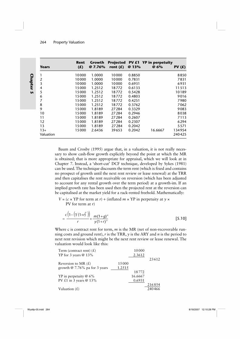
DCF valuation: Using the implied growth rate formula (Equation 5.7), the
annual growth rate implied from a target rate of 13% and an initial yield of
6% assuming 5-year rent reviews is 7.76% per annum.
Wyattp-05.indd 263Wyattp-05.indd 263 8/18/2007 12:10:28 PM8/18/2007 12:10:28 PM
264 Property Valuation
Ch
apter 5
YearsRent (£)
Growth @ 7.76%
Projected rent (£)
PV £1 @ 13%
YP in perpetuity @ 6% PV (£)
1 10 000 1.0000 10 000 0.8850 8 8502 10 000 1.0000 10 000 0.7831 7 8313 10 000 1.0000 10 000 0.6931 6 9314 15 000 1.2512 18 772 0.6133 11 5135 15 000 1.2512 18 772 0.5428 10 1896 15 000 1.2512 18 772 0.4803 9 0167 15 000 1.2512 18 772 0.4251 7 9808 15 000 1.2512 18 772 0.3762 7 0629 15 000 1.8189 27 284 0.3329 9 08310 15 000 1.8189 27 284 0.2946 8 03811 15 000 1.8189 27 284 0.2607 7 11312 15 000 1.8189 27 284 0.2307 6 29413 15 000 1.8189 27 284 0.2042 5 57113+ 15 000 2.6436 39 653 0.2042 16.6667 134 954Valuation 240 425
Baum and Crosby (1995) argue that, in a valuation, it is not really neces-
sary to show cash-flow growth explicitly beyond the point at which the MR
is obtained; that is more appropriate for appraisal, which we will look at in
Chapter 7. Instead, a ‘short-cut’ DCF technique, developed by Sykes (1981)
can be used. The technique discounts the term rent (which is fixed and contains
no prospect of growth until the next rent review or lease renewal) at the TRR
and then capitalises the rent receivable on reversion (which has been adjusted
to account for any rental growth over the term period) at a growth-im. If an
implied growth rate has been used then the projected rent at the reversion can
be capitalised at the market yield for a rack-rented freehold. Mathematically:
V = (c × YP for term at r) + (inflated m × YP in perpetuity at y ×
PV for term at r)
r
c (1- (1 (1+r) ))n
+=y (1+ r ) n
m (1+ g) n
[5.10]
Where c is contract rent for term, m is the MR (net of non-recoverable run-
ning costs and ground rent), r is the TRR, y is the ARY and n is the period to
next rent revision which might be the next rent review or lease renewal. The
valuation would look like this:
Term (contract rent) (£) 10 000YP for 3 years @ 13% 2.3612
23 612Reversion to MR (£) 15 000growth @ 7.76% pa for 3 years 1.2515
18 772YP in perpetuity @ 6% 16.6667PV £1 in 3 years @ 13% 0.6931
216 854Valuation (£) 240 466
Wyattp-05.indd 264Wyattp-05.indd 264 8/18/2007 12:10:28 PM8/18/2007 12:10:28 PM

Property Investment Valuation 265
Ch
apte
r 5
Unlike the ARY-based term and reversion technique the short-cut DCF
technique shows the correct capital values of the term and reversionary
incomes and reveals the growth assumption over the term. It is explicit about
the target rate and growth rate up to the first rent review, at which point the
MR (which has been projected at the long-term implied growth rate) is capi-
talised at the ARY. For properties where the cash-flow is more complex and
comparable evidence more scarce, a full DCF is perhaps more appropriate
but can lead to greater variability between valuers regarding values of key
input variables (Havard, 2000).
It is possible to use the implied rental growth rate formula to derive a
growth rate that is implied from the ARY, TRR and rent-review period of
a reversionary freehold property investment. The mathematics is a little
more complex but Brown and Matysiak (2000) provide a clear explana-
tion. Diagrammatically the situation is illustrated in Figure 5.3. The core and
top-slice ARY model (with equivalent yields) for calculating the PV of this
investment is adapted from Equation 3.3 in Chapter 3:
V = (c × YP into perpetuity) + ((m – c) × YP in perpetuity × PV for term)
V
cy
m cy (1+y) n
= + -
[5.11]
Where y is the equivalent ARY and the other variables are as defined for
Equation 5.10. The ARY implies growth and therefore the rent is not explic-
itly projected at the growth rate g. The DCF model does project rent at
the growth rate but, unlike a rack-rented property, there are two periods to
Figure 5.3 Rental growth between rent reviews.
Rental growthrate, g % pa
Rent-reviewperiod, p
MR atvaluation
date
MR(1 + g)n atfirst rentreview
Period to next rent review, n
Rent reviews
Time (years)
Contractrent, c
Leasestart
Valuationdate
0 3 5 10 15
Pre
sent
val
ue (
£)
Wyattp-05.indd 265Wyattp-05.indd 265 8/18/2007 12:10:30 PM8/18/2007 12:10:30 PM

266 Property Valuation
Ch
apter 5
incorporate into the calculation; one that lasts until the first rent review and
then the normal rent review period thereafter:
V
r= +
È
ÎÍÍ
˘c (1-(1 (1+r)n))˚̊˙˙r (1+r)n
m (1+g)n
(1+r)p - (1+r)p
(1+r)p -1
[5.12]
Where n is the period to the next rent revision and p is the rent review period.
If we assume that the PVs from each model produce the same answer we can
calculate the implied growth rate for a reversionary property investment. To
see how this works, take an example where the ARY is 8%, the TRR is 12%,
the rent review period is 5 years (for a rack-rented property investment the
growth rate implied by these figures would be 4.63% per annum) but the
period to next review is 2 years. The contract rent is £8 000 per annum and
the current MR is £10 000 per annum. An ARY core and top-slice technique,
using equivalent yields, produces the following valuation:
V = ++
80000 08 0 08 1 0 08 2. . ( . )
10000 - 8000 = 100000 + 21433 = £121433
If we assume that a DCF valuation should produce the same valuation, using
spreadsheet iteration in the final stage, g can be calculated as follows:
121 433 =c (1- (1 (1+ r) ))n
+r
n È
ÎÍÍ
˘
˚˙˙
0.15050 7623.È
ÎÍÍ
˘
˚˙˙
121 433 = 13 520 +
\ g = 0.0455 = 4.55%
m (1+ g)n
r (1+ r)
p (1+ g) -1
p p(1+ r) - (1+ g )2
10 1000(1+ g)5
1.7623 - (1+ g)
Therefore the implied growth rate from this reversionary property is slightly
lower than from the rack-rented equivalent because the rental growth will
arrive sooner due to the rent review in 2 years’ time rather than in 5 years.
5.2.3.3 Leasehold property investments
Baum and Crosby (1995) argue that a leasehold property investment pro-
ducing a fixed profit rent over its entire term produces a risk that is almost
entirely dependent upon the quality of the sub-tenant: a cash-flow from a
good quality tenant is similar to the return from a fixed income bond plus a
suitable risk premium. The target rate used to discount a fixed profit rent is
therefore likely to be derived from comparison to other fixed income invest-
ments such as gilts with similar maturity dates. This approach is more logical
and is not based on questionable comparisons with the freehold investment
market (see Chapter 3).
If the profit rent is variable then there is a gearing effect. Basically if a
fixed head-rent is deducted from a sub-rent which includes rent reviews the
resultant profit rent must vary by an amount greater than the variation in
Wyattp-05.indd 266Wyattp-05.indd 266 8/18/2007 12:10:30 PM8/18/2007 12:10:30 PM

Property Investment Valuation 267
Ch
apte
r 5
the sub-rent itself. The magnitude of this variability depends on the size of the
fixed deduction of head-rent from the variable sub-rent and can be expressed
as the income-gearing ratio. To illustrate this consider three property invest-
ments; a freehold, a leasehold where the head-rent is very similar to the sub-
rent and another leasehold where the sub-rent is very much larger than the
head-rent. All three investments generate an initial income of £100 000 per
annum subject to annual rent reviews and rental growth is estimated to be
5% per annum. As can be seen from Table 5.5 the income from the freehold
investment grows at the rental growth rate of 5% per annum. The first lease-
hold investment receives a £900 000 per annum sub-rent and pays a £800 000
per annum head rent, leaving £100 000 per annum profit rent. The second
leasehold receives a £110 000 per annum sub-rent and pays a £10 000 per
annum head rent, leaving £100 000 per annum profit rent.
Except where the head rent is a peppercorn (very low) rent, rental growth
for a leasehold profit rent is greater than the rental growth on an equiva-
lent freehold. The growth rate diminishes at each subsequent rent review
and tends towards the market rental growth rate in perpetuity (Baum and
Crosby, 1995). The income-gearing ratio for the first leasehold is 89% and
for second it is 9%. Life becomes a whole lot more complicated as we intro-
duce asynchronous rent reviews in the head- and sub-leases. So the way
Table 5.5 Geared leasehold profi t rents.
Year
Freehold initial net income (£)
Freehold income
growth (%)
Leasehold 1 initial net income (£)
Leasehold 1 income
growth (%)
Leasehold 2 initial net income (£)
Leasehold 2 income
growth (%)
0 100 000 — 100 000 — 100 000 —1 105 000 5.00 145 000 45.00 105 500 5.502 110 250 5.00 192 250 32.59 111 275 5.473 115 763 5.00 241 863 25.81 117 339 5.454 121 551 5.00 293 956 21.54 123 706 5.435 127 628 5.00 348 653 18.61 130 391 5.406 134 010 5.00 406 086 16.47 137 411 5.387 140 710 5.00 466 390 14.85 144 781 5.368 147 746 5.00 529 710 13.58 152 520 5.359 155 133 5.00 596 195 12.55 160 646 5.3310 162 889 5.00 666 005 11.71 169 178 5.31...40 703 999 5.00 5 535 990 5.76 764 399 5.0741 739 199 5.00 5 852 789 5.72 803 119 5.0742 776 159 5.00 6 185 429 5.68 843 775 5.0643 814 967 5.00 6 534 700 5.65 886 463 5.0644 855 715 5.00 6 901 435 5.61 931 287 5.0645 898 501 5.00 7 286 507 5.58 978 351 5.0546 943 426 5.00 7 690 832 5.55 1 027 768 5.0547 990 597 5.00 8 115 374 5.52 1 079 657 5.0548 1 040 127 5.00 8 561 143 5.49 1 134 140 5.0549 1 092 133 5.00 9 029 200 5.47 1 191 347 5.0450 1 146 740 5.00 9 520 660 5.44 1 251 414 5.04
Wyattp-05.indd 267Wyattp-05.indd 267 8/18/2007 12:10:32 PM8/18/2007 12:10:32 PM

268 Property Valuation
Ch
apter 5
that a profit rent might be expected to grow depends on the income-gearing
ratio. Use of an ARY technique (even the single rate approach described
in Chapter 3) is hard to justify because of heterogeneity of interests and
potential complexity profit rent cash-flows. Similarly, identifying a market
TRR for leaseholds with variable and geared profit rents is difficult as each
investment opportunity will have unique ratios between head-rent and sub-
rent leading to individual profit rent cash-flows and gearing circumstances.
Furthermore, there will be differences in tenant quality and remaining lease
term. The leasehold target rate must relate to the lease structure and any
profit rent gearing and Baum and Crosby (1995) suggest that attention
should focus on the choice of risk premium when moving from a freehold to
a leasehold target rate. Other cash-flow variables such as the head-rent, rent
reviews and so on can also be incorporated in the cash-flow.
Freehold investment transactions can be analysed to derive a suitable
rental growth rate which can be applied to the leasehold investment cash-
flow and this should be done in preference to estimating a growth rate that
is implied by the relationship between target rate and ARY on a leasehold
investment because of the heterogeneity of cash-flows from leasehold invest-
ments (Baum and Crosby, 1995). If the leasehold includes a head rent and
sub-rent both with rent reviews at the same time and both rents are assumed
to grow at the same rate, then the profit rent would grow at the same rate
as the growth in MR for a freehold. But in cases where the rent reviews in
the sub-lease (say every 5 years) are different to those in the head-lease (say
every 15 years) the complexities are best handled by a full DCF rather than
a short-cut. As an example the leasehold investment described in Section
3.3.3 of Chapter 3 will be valued again but this time using a DCF technique.
Assuming a target rate of 10% and an ARY of 6% for freehold property
this implies rental growth of 4.47% per annum. But the target rate at which
the cash-flow from a leasehold investment is discounted must be adjusted to
reflect additional risk. Here the adjustment is from 10% to 15%.
YearsRent received (£)
Growth @ 4.47% pa
Infl ated rent (£)
Less rent paid (£)
Profi t rent (£)
PV @ 15% PV (£)
1 30 000 1.0000 30 000 –10 000 20 000 0.8696 17 3922 30 000 1.0000 30 000 –10 000 20 000 0.7561 15 1223 35 000 1.0913 38 196 –10 000 28 196 0.6575 18 5394 35 000 1.0913 38 196 –10 000 28 196 0.5718 16 1225 35 000 1.0913 38 196 –10 000 28 196 0.4972 14 0196 35 000 1.0913 38 196 –10 000 28 196 0.4323 12 1897 35 000 1.0913 38 196 –10 000 28 196 0.3759 10 5998 35 000 1.3578 47 523 –10 000 37 523 0.3269 12 2669 35 000 1.3578 47 523 –10 000 37 523 0.2843 10 66810 35 000 1.3578 47 523 –10 000 37 523 0.2472 9 27611 35 000 1.3578 47 523 –10 000 37 523 0.2149 8 06412 35 000 1.3578 47 523 –10 000 37 523 0.1869 7 013Valuation 151 269
Wyattp-05.indd 268Wyattp-05.indd 268 8/18/2007 12:10:32 PM8/18/2007 12:10:32 PM

Property Investment Valuation 269
Ch
apte
r 5
5.2.4 Case study – valuation of a city centre offi ce block
You have been asked to value, for sale purposes, the freehold and head-leasehold interests in the property described below. The valuation date is the 1 April 2005. The property was constructed in 1980 and is located in the central business district of Bristol. It comprises a basement (used for storage) with five floors above (including the ground floor). Externally, notable fea-tures include glazed exterior cladding, a high quality entrance and reception area on the ground floor and a secure barrier to the car park at the rear. The office accommodation is open plan and finished to a reasonable specification (suspended ceilings and perimeter trunking but no air-conditioning or raised floors). There are two lifts serving all floors. Car parking is rather restricted due to the location of the property in the centre of the city but access to the railway station and main bus routes is good. The property is also close to the main retail area of the city. Occupying tenants can internally partition the floor-space under the terms of the leases. With regard to maintenance of the building, each occupying tenant pays a portion of the annual service charge to the landlord. The floor area that each tenant occupies is used to apportion the service charge between tenants. The service charge pays for the cleaning of common parts, general repairs, services, lighting to common parts, lifts, insurance and management. The tenants pay for their own cleaning and lighting.
5.2.4.1 Head-lease
Y is the landlord of the site which was let to Z on a 125-year-ground lease
in 1988. The initial rent that was agreed was £10 000 per annum and the
landlord has no responsibility for the insurance or repairs of the office build-
ing on the site. The rent payable under the ground lease is reviewed every 25
years. At each review the rent is reviewed to the existing ground rent plus 5%
of the estimated market rental value of the head-lease in excess of the existing
ground rent. The wording of the rent review clause in the ground-lease per-
mits the head-lease to be valued assuming the building is vacant and to let.
5.2.4.2 Occupational sub-leases
All of the occupational sub-leases specify that the sub-tenants are responsi-
ble for all repairs and insurance (non-internal repairs and insurance payable
via the service charge) and are subject to 5-year, upward-only rent reviews.
Table 5.6 lists the details of the sub-leases.
Each occupying sub-tenant must pay a portion of the annual service charge,
itemised in Table 5.7.
This total service charge per square metre is then apportioned between the
sub-tenants on a floor area basis with a reduction of 50% for the basement
store. The apportioned charges are listed in Table 5.8.
After a review of your firm’s internal records and discussions with col-
leagues at other surveying firms in the city, three properties have recently
Wyattp-05.indd 269Wyattp-05.indd 269 8/18/2007 12:10:33 PM8/18/2007 12:10:33 PM

270 Property Valuation
Ch
apter 5
been the subject of transactions that provide comparable evidence for your
subject property:
(a) The basement of the office building next door was recently let to the pub-lishers (who occupy the fourth floor of the subject property) for additional archiving and general storage. The lease was agreed on standard terms for a period of 5 years at a rent that equated to £90 per square metre.
Table 5.6 Sub-leases.
Floor Tenant Use Business CovenantaArea (m2)
Current rent (£)
Date lease commenced
Length of lease (years)
Basement A Store Solicitors Good 305 21 350 1997 15Ground A Offi ce Solicitors Good 251b 40 160 2003 10First B Offi ce Insurance Good 449 76 330 2005 15Second C Offi ce Travel Poor 449 49 390 1988 25Third D Offi ce Surveyors Average 449 69 595 2000 10Fourth E Offi ce Publishers Poor 398 55 720 1997 15Totals 2301 312 545
aThe covenant describes the quality of the tenant in terms of ability to meet the terms of the lease. It is a subjective measure of the security of the income.bEntrance and reception areas are on this fl oor.
Table 5.7 Service charge details.
Item Cost (£/m2)
Staff 3.50Cleaning of common parts 2.00General repairs 5.00Services 2.75Lighting to common parts 1.25Lifts 2.75Insurance 2.75Management 2.50Total 22.50
Table 5.8 Service charge apportionment.
Floor Sub-tenant Use Area (m2) Service charge (£)
Basement A Store 305 3 431.25Ground A Offi ce 251 5 647.50First B Offi ce 449 10 102.50Second C Offi ce 449 10 102.50Third D Offi ce 449 10 102.50Fourth E Offi ce 398 8 955.00
Wyattp-05.indd 270Wyattp-05.indd 270 8/18/2007 12:10:33 PM8/18/2007 12:10:33 PM

Property Investment Valuation 271
Ch
apte
r 5
This provides evidence of the current MR for storage space in this type of building.
(b) The letting of the first floor of the subject property to the insurance
company was recent and was agreed on standard terms. It therefore
provides good evidence of the current MR for the office space. The rent
agreed equates to £170/m2.
(c) The fifth (top) floor of the office building next door was recently let
on standard terms. The lease was for a term of 15 years at a rent that
equates to £150/m2. However, on inspection of this building it is noted
that the lift only goes up to the fourth floor and clearly a reduction to
the ‘normal’ MR for office space in this area has been made to take this
into account.
It is decided that the comparable evidence in (c) will be classed as second-
ary due to the poor lift access. Thus the current MR for office space in this
locality is estimated to be £170/m2. Table 5.9 shows the current and esti-
mated MRs for each sub-lease.
5.2.4.3 Valuation of the freehold interest
Term rent (£) 10 000YP 8 years @ 8% 5.7466
57 466Reversion to MR of head-lease (£) 366 770less rent passing (£) −10 000
356 7705% share of MR 0.05
17 839
Table 5.9 Current and full rental values of the sub-leases.
Floor TenantDate lease
commenced
Length of lease (years)
Current rent (£)a
Next rent review
Current market
rent (£)b
Basement A 1997 15 21 350 2007 27 450Ground A 2003 10 40 160 2000 42 670First B 2005 15 76 330 2002 76 330Second C 1988 25 49 390 2000 76 330Third D 2001 10 69 595 1998 76 330Fourth E 1997 15 55 720 1999 67 660Totals 312 545 366 770
a MR is not received until fi rst rent review for each sub-lease.b The comparable evidence of market rents for storage and offi ce space are used to calculate the rental values for each fl oor of the subject property.
Wyattp-05.indd 271Wyattp-05.indd 271 8/18/2007 12:10:34 PM8/18/2007 12:10:34 PM

272 Property Valuation
Ch
apter 5
plus rent passing (£) 10 00027 839
YP in perpetuity @ 10% 10.000PV £1 for 8 years @ 10% 0.4665
129 871Valuation (£) 187 337
5.2.4.4 Valuation of the head-leasehold interest
Valuing year-by-year until the rent on each floor is reviewed to market rental
value and incorporating the review of the ground rent, the valuation below
has been set out as a cash-flow. Given the long length of the ground-lease
(125 years) and the relatively low ground rent (currently £10 000) this inter-
est will be valued as though it were a freehold. The difference is negligible;
the YP for the remainder of the ground lease (108 years) at 11% is 9.0906
whereas the YP in perpetuity at 11% is 9.0909.
Year
Rent received
(£)Ground rent (£)
Profi t rent (£)
YP in perpetuity
@ 11%PV £1 @ 11% PV (£)
2005 312 545 10 000 302 545 0.9009 272 5632006 319 280 10 000 309 280 0.8116 251 0182007 337 320 10 000 327 320 0.7312 239 3272008 366 770 10 000 356 770 0.6587 235 0042009 366 770 10 000 356 770 0.5935 211 7432010 366 770 10 000 356 770 0.5346 190 7292011 366 770 10 000 356 770 0.4817 171 8562012 366 770 10 000 356 770 0.4339 154 8022013 366 770 27 839 338 931a 9.0909 0.3909 1 204 436Valuation £2 931 480
aThis rent is receivable for the remainder of the ground-lease (assumed to be in perpetuity) and is capitalised at a yield of 11% but deferred 9 years.
The main decision that a valuer must make is the choice of yield. Although
this long leasehold interest is, in many ways, similar to a freehold inter-
est, it is ultimately a wasting asset and is usually not as desirable as a free-
hold investment. The yield should reflect such market perception as well as
opportunity cost of capital, potential for growth and a return for risk taken.
Yield choice is always difficult and is particularly so with interests such as
this where comparable evidence is hard to obtain. In practice different yields
may be applied to the capitalisation of the various rental income streams.
For example, a higher yield may be adopted for the capitalisation of the
reduced profit rent receivable after the review of the ground rent in 2013.
Similarly, different yields may be chosen depending on which sub-tenant the
rental income originates from. This may help to reflect the security value of
each portion of the rental income.
Wyattp-05.indd 272Wyattp-05.indd 272 8/18/2007 12:10:34 PM8/18/2007 12:10:34 PM

Property Investment Valuation 273
Ch
apte
r 5
Key points
The value of an investment can be considered to be a multiple of the cur rent rent where the multiplier is the reciprocal of the investor’s required income yield (ARY valuation technique) or the PV of the expected future cash-flow (DCF valuation technique) (Fraser, 1993). Techniques vary depending on the extent to which assumptions are made explicit. For example a valuer may wish to include an explicit growth rate forecast rather than imply a long-term average from analysis of comparable evidence, or depreciation may be explic-itly accounted for in the cash-flow. The problem with being more explicit is that there is greater potential for valuation variance (Havard, 2000).
The ARY model does not explicitly reveal the total return that an investor expects; instead, future rental income is discounted (capitalised) at a rate that implies that the investor expects the income to grow in order to achieve a TRR. The DCF model involves selecting a suitable holding period, forecast-ing the cash flow over this period and selecting an appropriate target rate and exit yield. All of these assumptions should reflect market behaviour so valuers need to interpret activities and expectations of market participants (Appraisal Institute, 2001).
The DCF technique is better at isolating factors affecting future income flow from those that affect the TRR required by the investor, thus allowing direct comparison with other investment opportunities. It can also deal with com-plexity and reveal assumptions explicitly. In cases where a property presents a non-standard pattern of income a DCF approach will usually be preferable. For example, investments with a ground lease and an occupational lease granted at different times, phased development projects or leaseholds where the head-lease has infrequent reviews and the sub-lease does not, the DCF approach provides more information and helps focus attention on fundamental charac-teristics that the investor will be interested in, namely income growth, depre-ciation, the holding period, timing of income and expenditure and the TRR. Rent tends to be subject to depreciation and capital values to obsolescence and the effect of these can be handled explicitly by adjusting the rental growth rate and exit yield or implicitly by adjusting the TRR (Sayce et al., 2006).
Choice of method is a matter of availability of evidence and complexity of the property interest being valued: use the ARY technique when investments have a standard pattern of income and rent reviews, use the DCF technique for complex interests, long reversions and short leaseholds. When valuing leasehold investments complex gearing effects are much more suited to detailed cash-flow analysis rather than simple yield capitalisation.
5.3 Valuing contemporary property investments using ARY and DCF valuation techniques
At the end of the last section the case was made for using a DCF technique
to value properties with particular investment characteristics that render the
ARY technique inadequate. These characteristics include properties that are
over-rented, let on short leases or on leases that contain break clauses. A DCF
technique might also be employed to analyse transactions where properties
have not been let at MR (perhaps because an incentive such as a rent-free
Wyattp-05.indd 273Wyattp-05.indd 273 8/18/2007 12:10:35 PM8/18/2007 12:10:35 PM

274 Property Valuation
Ch
apter 5
period or capital inducement was offered) so that they can be used as com-
parable evidence. In all of these cases the overriding concern to the landlord
is that the financial position is adequate for the option or incentive granted.
The number of property investments subject to flexi-leases is increasing and
Table 5.10 shows the percentage of tenancies monitored by IPD that were
over-rented and void in 2004.
Table 5.10 Over-rented and void tenancies at the end of 2004 by market segment.
Market segment % tenancies over-rented % tenancies void
Standard shops 18.5 7.2 Central London 25.2 9.4 Rest of London 14.7 5.9 South East and Eastern 22.0 5.8 Rest of UK 15.6 7.4Shopping centres 17.3 6.8 In-town 17.6 7.2 Out-of-town 15.5 4.3Retail warehouses 6.8 4.8 Retail parks 7.1 4.0 Fashion parks 6.3 5.9 Other retail warehouses 6.3 6.4Dept/variety stores 11.6 14.7Supermarkets 10.7 5.3Other retail 18.6 5.0Standard offi ces 38.2 15.8 Central London 44.6 16.7 Rest of London 44.7 16.1 Inner South Eastern 54.4 15.2 Outer South Eastern 35.4 14.7 Rest of UK 20.5 14.6Offi ce parks 43.1 16.4 London and South Eastern 52.0 20.3 Rest of UK 27.6 9.4Standard industrials 25.3 11.6 London 19.9 9.5 Inner South Eastern 27.5 11.2 Outer South Eastern 31.5 11.6 Rest of UK 23.0 12.4Distribution warehouses 20.4 6.0Other property 10.1 7.1 Leisure 14.4 11.0All retail 16.1 6.7All offi ce 38.7 15.8All industrial 25.1 11.5All property 22.8 9.7
Source: IPD UK Digest (2005).
Wyattp-05.indd 274Wyattp-05.indd 274 8/18/2007 12:10:35 PM8/18/2007 12:10:35 PM

Property Investment Valuation 275
Ch
apte
r 5
This section looks at how ARY and DCF valuation techniques can be
used to value property investments subject to flexi-leases and over-rented
properties.
5.3.1 Short leases and leases with break clauses
Short leases and leases with break options, collectively referred to as flexi-
leases (see Chapter 4), mean greater diversity of lease contracts and increased
uncertainty for investors. Will the tenant renew the short lease? If not will
there be a rent void and how long might it be? What will the lease terms
be and what will be the quality of the new tenant? Will a break option be
exercised? All this uncertainty creates an income risk that an investor will
wish to be compensated for in terms of price paid and the expected return.
McAllister (2001) argues that the capital value of a contemporary property
investment is dependent upon the cost and probability of the tenant vacat-
ing, a rent void occurring or the rent dropping, and the impact on value will
depend on the length of the short lease, the structure of the break clause
(specifically the terms of any penalty payment), the tenant’s business plan
and market factors (such as rental growth prospects and the state of the
lettings market).
Before flexi-leases became commonplace homogeneity of lease contracts
meant that, for property investment valuation, adjustments to initial yields
of comparables to reflect geographical and physical differences could be jus-
tified. But now it is much harder to find comparables and justify small but
often cumulative adjustments to the ARY because of the greater variety of
possible differences between the subject property and each comparable. ARY
adjustment is, therefore, an over-simplification and it is difficult to quantify
and support; a more explicit approach is required to illustrate the reasoning
behind the assumptions (Crosby et al., 1998). The DCF technique allows
assumptions to be made more clearly; the financial costs (and possible ben-
efits) associated with the exercise of a break option or non-renewal of a
lease and the possible void period that may follow for example. Research
has revealed errors and a lack of consistency amongst valuers when valuing
flexi-leases (see McAllister and O’Roarty, 1999; Ward and French, 1997).
Valuers tend to focus on the worst-case scenario and assume that there will
be a rent void at the end of the (short) lease or that a break option will be
exercised. This is despite the fact that if the out-going tenant had to pay
a penalty fee (equivalent to several months’ rent) and a new tenant was
found in the meantime the landlord may actually receive an income bonus.
This conservative approach tends to undervalue flexi-leases and reduce their
attractiveness to investors.
Consider the following example: a modern office property has just been
let on a 15-year FRI lease at a MR of £50 000 per annum with no rent
reviews. There is a break option in the tenant’s favour in year 5, just before
the rent review (to prevent the tenant from using it as a bargaining tool).
Comparable evidence suggests that rack-rented office investments let on
15-year FRI leases with 5-year rent reviews to MR sell at prices that generate
Wyattp-05.indd 275Wyattp-05.indd 275 8/18/2007 12:10:35 PM8/18/2007 12:10:35 PM

276 Property Valuation
Ch
apter 5
initial yields of around 7%. Long-term gilts currently yield 8% and a typical
property risk premium is 2%. The inclusion of a break option clearly adds a
degree of uncertainty to the income that the investor would receive after year
5. Indeed, an early break will have a greater impact on capital value than a
later one due to the time value of money (Havard, 2000). Possible outcomes
at the break are; the tenant exercises the break and a rent void follows, the
break is exercised but there is no void, or the tenant continues in occupation.
Faced with such uncertainty the valuer might increase the ARY slightly on
the assumption that the break will definitely be exercised (French, 2001).
Here the ARY has been increased from 7% to 8%.
MR (£) 50 000YP perpetuity @ 8% 12.5Valuation (£) 625 000
If the lease had no break option and was valued using a 7% yield the capital
value would be £714 286, so the yield adjustment leads to a 12.5% reduction in
value. This approach is simple and benefits from a direct relationship with com-
parable evidence, assuming there is a sufficient amount available, but it hides
a lot of assumptions (Havard, 2000). Another approach might be a modified
term and reversion valuation where the ARY is adjusted by a lesser amount and
a rent void is incorporated in the cash-flow after the break. The valuer needs to
be sure (via market evidence) that the void duration is realistic. An advantage of
this approach is that different yields can be used for the existing and new leases
(Havard, 2000) but, again, only if justified by market evidence. The valuation
below incorporates a void period of 1 year after the break option in year 5 and,
in order to avoid double-counting, the yield has only been adjusted upwards to
7.5%. Clearly this results in a more optimistic valuation.
MR – fi rst lease (£) 50 000YP 5 years @ 7.5% 4.0459
202 950MR – new lease (£) 50 000YP perpetuity @ 7.5% 13.33PV 6 years @ 7.5% 0.6480
432 000Valuation (£) 634 950
It is useful to look at the level of rental growth as a guide to the likeli-
hood of the rent dropping at the time a break option might be exercised.
The short-cut DCF valuation is explicit about the target rate and the growth
rate and accurately values each part of the income flow in a reversionary
investment. Havard (2000) argues that the target rate would probably need
to be increased to reflect the added risk associated with investing in a short
lease. The problem is that there are now a lot of assumptions to make and
this could lead to increased valuation variance. Similarly a full (year-by-year)
DCF valuation is even more explicit about assumptions and therefore
may lead to even greater valuation variance; changes to each key variable
Wyattp-05.indd 276Wyattp-05.indd 276 8/18/2007 12:10:36 PM8/18/2007 12:10:36 PM

Property Investment Valuation 277
Ch
apte
r 5
(growth rate, exit yield, target rate, void period, holding period) in isola-
tion have little impact on the valuation but taken together they do (Havard,
2000). Assuming a TRR of 10% and an ARY of 7.5%, this implies a growth
rate of 2.88% per annum. A full DCF valuation of a short lease with a break
clause is shown below. On a standard lease a rent of £50 000 per annum and
a yield of 7.5% would produce a valuation of £666 667.
YearNet cash-fl ow (£)
Implied growth rate
of 2.88%Estimated
cash-fl ow (£)
PV £1 @ target rate
of 10%Discounted income (£)
1 50 000 1.0000 50 000 0.9091 45 4552 50 000 1.0000 50 000 0.8264 41 3223 50 000 1.0000 50 000 0.7513 37 5664 50 000 1.0000 50 000 0.6830 34 1515 50 000 1.0000 50 000 0.6209 31 0466 0 0.0000 0 0.0000 07 50 000 1.1857 59 286 0.5132 30 4238 50 000 1.1857 59 286 0.4665 27 6589 50 000 1.1857 59 286 0.4241 25 14310 50 000 1.1857 59 286 0.3855 22 85811 50 000 1.1857 59 286 0.3505 20 78011-perp. 50 000 1.3666 911 065 0.3505 319 323Valuation (£) 13.3333 635 723
A difficulty with these modified ARY and DCF approaches is their inabil-
ity to handle the possibility that the break option is not exercised (or if it is
and there is no rent void). Under this assumption, in terms of the cash-flow,
the flexi-lease is no different from a standard lease but because of the yield
adjustment and void assumption the landlord will receive a financial bonus
in comparison to a standard lease. The problem is uncertainty; the cash-
flow has been made more uncertain by the flexi-lease and this uncertainty
has a price. The dilemma for the valuer is trying to estimate that price. One
solution to this problem is to produce a range of valuations under differ-
ent scenarios; the break clause is/is not exercised, the rent void does/does
not occur, a void lasts for 6 months, 1 year, and so on. This leads to a lot of
valuations and, as a way of summarising the various outcomes, probabilities
could be assigned to them and a weighted average ‘expected’ valuation cal-
culated (French, 2001). It is possible to extend this simple ‘discrete’ probabil-
ity analysis into a continuous probability analysis using simulation or option
pricing and we will look at these approaches in Section 5.4.
5.3.2 Over-rented property investments
Over-renting occurs when the rent payable under a lease with upward-only
rent reviews exceeds the MR. Some valuers value over-rented properties as
perpetual cash flows at the passing rent when the lease is long, contains
upward-only rent reviews and no break clause. Because of the higher risk
Wyattp-05.indd 277Wyattp-05.indd 277 8/18/2007 12:10:36 PM8/18/2007 12:10:36 PM

278 Property Valuation
Ch
apter 5
associated with the element of rent that exceeds the MR, known as the over-
age or froth, other valuers use a layer (core and top-slice) approach, using
an ARY based on rack-rented freehold comparables to capitalise the core
rent (which is taken to be the MR at the time of the valuation) and a fixed
income yield that reflects the covenant strength of the tenant to capitalise the
top-slice or ‘overage’.
For example, value a property let 4 years ago at a rent of £250 000 per
annum on a 15 year lease with 5 year upward-only rent reviews. The current
MR is £200 000 per annum. Comparable properties have recently sold for
yields averaging 6%. Medium-dated gilts are yielding 5% and the investor’s
TRR for this property is 11%. The ARY (core and top-slice) valuation is as
follows:
Core (market) rent (£) 200 000 YP in perpetuity @ 6% 16.6667
3 333 340Top-slice (overage) (£) 50 000YP 11 years @ 7%a 7.4987
374 935Valuation (£) 3 708 275
aGilt yield plus a 2% risk premium.
However, there are problems with this approach: first, the core rent is capi-
talised at an ARY that assumes 5 years to the next review but the property is
reversionary and the growth potential is closer – consequently the approach
over-values the bottom layer; second, there is a lack of evidence on which
to base the overage yield; and third, no attempt has been made to estimate
the length of time that the property will remain over-rented. To resolve the
last problem many valuers capitalise the overage for the whole period that
the tenant is contracted to pay it (Crosby and Goodchild, 1992). But if, as
Martin (1991) points out, the MR grows each year and the overage reduces,
the MR may overtake the contract rent before the end of the lease and part
of the overage is capitalised twice – the property will be over-valued. This is
illustrated in the Figure 5.4.
Even if the overage is capitalised until the first rent review after the MR
overtakes the contract rent a (smaller) amount of double-counting still
occurs. The layer approach is unable to calculate the corresponding reduc-
tion in the overage necessary to avoid this double-counting. One way to
resolve this problem is to be explicit about growth in the rental income and
project the MR at a growth rate to determine when it will overtake the con-
tract rent. This growth rate can be implied from the relationship between the
chosen ARY and target rate or it can be explicitly forecast. A DCF approach
can then be used to capitalise the contract rent up to this cross-over point (or
the next review thereafter) at the target rate and the uplifted MR is capital-
ised at an ARY from the cross-over point into perpetuity, discounted for the
period of waiting, at the target rate – just like a short-cut DCF.
Wyattp-05.indd 278Wyattp-05.indd 278 8/18/2007 12:10:36 PM8/18/2007 12:10:36 PM

Property Investment Valuation 279
Ch
apte
r 5
Continuing the example above, using a growth rate of 5.57% per annum,
implied from the ARY of 6% and the target rate of 11%, the MR will grow
to the following amounts at the next two rent reviews:
£200 000 × (1+0.0557)1 = £211 140
£200 000 × (1+0.0557)6 = £278 868
So the MR overtakes the contract rent between the first and second rent
reviews and the growth-explicit short-cut DCF valuation is as follows:
Term (contract rent) (£) 250 000YP 6 years @ 11% 4.2305
1 057 625Reversion to MR (£) 200 000FV 6 years @ 5.57% 1.3843YP in perpetuity @ 6% 16.6667PV 6 years @ 11% 0.5346
2 466 828Valuation (£) 3 524 453
The valuation is lower than the layer approach above because the double-
counting has not occurred and the use of a target rate to capitalise the term
rent means that the problem of using a rack-rented ARY to value a bot-
tom layer where the reversion is closer does not arise. A drawback of the
growth-explicit DCF approach is the lack of comparable evidence to support
the choice of rental growth rate and TRR which may need to be adjusted
to reflect the covenant strength of the tenant, the length of the remaining
lease term and the extent of the overage (Crosby, 1991). In between rent
reviews rent is only subject to tenant (default) risk and if the contract rent is
very high in comparison to MR for long periods (e.g. beyond the first rent
review) then it is exposed to a greater degree of tenant risk. As such it may be
Ren
t
Projectedmarket rent
(End of lease)
Time (years)
Contractrent
Currentmarket
rent
Top layer capitalised at overage yield
0 1 6 11
Bottom layer capitalised at ARYIncome that is capitalised twice
Figure 5.4 Over-rented property.
Wyattp-05.indd 279Wyattp-05.indd 279 8/18/2007 12:10:36 PM8/18/2007 12:10:36 PM

280 Property Valuation
Ch
apter 5
more characteristic of a corporate bond-type investment issued by the tenant
(Brown and Matysiak, 2000).
A property let at a headline rent is, in effect, over-rented and should, argu-
ably, be valued as such. Revisiting the property described in the Section 4.2.1
on rent-free periods in Chapter 4, assume that a write-off period of 15 years
(the lease term) is appropriate. This equates to a growth rate of 2.62% per
annum which we can insert as an explicit growth rate into the capital valua-
tion. If we also assume an ARY of 7% and a target rate of 10% the valuation
of the freehold investment interest using a short-cut DCF technique would
be as follows:
Headline rent (£) 200 000YP 13.5 years @ 10% 7.2382PV £1 1.5 years @ 10% 0.8668
1 254 814Reversion to MR (£) 175 721FV £1 15 years @ 2.62% pa 1.4739YP perpetuity @ 7% 14.2857PV £1 15 years @ 10% 0.2394
885 763Valuation (£) 2 140 577
To investigate the impact that the rent-free period has on capital value,
assume the property has no rent-free period (apart from the normal fitting
out period of 6 months), it is let at the real rent of £175 721 per annum
(calculated in Chapter 4) and the ARY is 7%:
MR (£) 175 721YP perpetuity @ 7% 14.2857PV 0.5 years @ 7% 0.9667Valuation (£) 2 426 705
For the valuation of the property let at MR to equate to the DCF valuation
of the property let with the rent-free period, the MR would have reduced
from £175 721 to £155 002 per annum. So, because of the yield impact on
capital value, incentives such as rent-free periods are preferable to reductions
in the headline rent (Crosby and Murdoch, 1994).
Key points
At the beginning of the twentieth century valuers would capitalise rent at an evidence-based initial yield. Initial yield evidence was obtained from the market and comparable to gilts plus a risk premium as there was no rental growth or inflation. By the mid-1970s rent reviews were introduced so that landlords could benefit from rising rents. The relationship between gilts and property yields was broken – property was now regarded as a growth
Wyattp-05.indd 280Wyattp-05.indd 280 8/18/2007 12:10:37 PM8/18/2007 12:10:37 PM

Property Investment Valuation 281
Ch
apte
r 5
5.4 Advanced property investment valuation techniques for dealing with uncertainy in valuations
5.4.1 Valuation accuracy, variance and uncertainty
Because of the market imperfections and inefficiencies in the property
market referred to in Chapter 1, the expertise and experience of a valuer
is required to form an opinion of value based on an assessment of value-
significant influences. These influences may change and therefore a valua-
tion is not a permanent part of the property. Analysis of market data only
suggests what happened in the past and it is for the valuer to interpret these
data to assess current market value. Valuers do not operate with perfect
market knowledge, they must follow client instructions, make judgements,
analyse information and respond to different pressures when preparing a
valuation and all these factors influence the final valuation figure. Values
can be difficult to assess due to the heterogeneity of property and the num-
ber of transactions that occur at prices that do not represent market values.
Although the profession has sought to enforce more rigorous mandatory
standards and practice statements, backed by detailed guidance notes,
Key points (continued)
investment like equities but with a peculiar income growth pattern. A simple initial yield approach was no longer appropriate, particularly for valuations between reviews, therefore term and reversion, hardcore and top-slice and equivalent yield methods were devised.
Structural changes in the economy during the 1990s brought about by low inflation, increased uncertainty, changing business structure, developments in ICT and globalisation led to a decrease in lease lengths, increased use of break clauses and other options, plus increased use of incentives. All of this leads to more complex valuations. Investors may now be faced with two options; investing in much shorter leases with break clauses or investing in sale and leasebacks to corporate occupiers. The latter may be 25-to 35-year leases and on inflation-linked rent reviews.
In terms of valuation there are problems with the ARY technique when valu-ing properties let on flexi-leases, over-rented property and properties not let at MR due to inducements. A short-cut DCF technique solves many of the problems associated with the ARY technique and is mathematically consis-tent and explicit regarding the target rate and growth assumptions, at least until the first review. Its inputs are also largely derived from market evidence and should therefore produce a market valuation (Havard, 2000).
With a full DCF, more assumptions have to be made and reliance on sim-ple market ratios and other information is reduced – the valuation starts to become an appraisal. Such a method may produce a wider variation of answers depending on the assumptions made. Consequently a full DCF may be appropriate when valuing complex properties with few comparables.
Wyattp-05.indd 281Wyattp-05.indd 281 8/18/2007 12:10:37 PM8/18/2007 12:10:37 PM

282 Property Valuation
Ch
apter 5
valuations of the same property conducted by different valuers will not
always be the same and the valuation(s) may not necessarily equate to the
agreed exchange price. The disparity in valuations of the same property
is referred to as valuation variance and the discrepancy between a valua-
tion figure and the exchange price is referred to as valuation inaccuracy.
Valuation uncertainty is a recently coined phrase used to acknowledge the
fact that valuation variance and valuation inaccuracy are inevitable conse-
quences of the valuation process and recent research has attempted to quan-
tify the degree of uncertainty that surrounds valuation. Market conditions
and the type and location of property investments will influence the degree
of uncertainty. There have been a number of studies that have investigated
the degree of valuation inaccuracy and extent of valuation variance that
occurs in typical property investment valuations and the Royal Institution
of Chartered Surveyors (RICS) has considered ways of reporting valuation
uncertainty when it is deemed appropriate.
5.4.1.1 Valuation accuracy
Brown (1985) examined the accuracy of valuations by regressing valuations
on exchange prices for 29 properties where the sale price and preceding
valuation were known and found a high correlation between valuations and
prices. In 1988 similar regression techniques1 were applied to a much larger
sample of 1442 valuations and sale prices taken from the IPD (IPD/Drivers
Jonas, 1988). This study and its update (IPD/Drivers Jonas, 1990) both found
that valuations and prices were highly correlated. There have, however, been
criticisms of the statistical validity of the regression analysis in these studies,
particularly in relation to the problem of heteroskedasticity2 (Lizieri and
Venmore-Rowland, 1991). A longitudinal study of the accuracy of valua-
tions is now funded by the RICS and conducted using IPD data. In 2004
RICS and IPD conducted an analysis of 984 valuations and subsequent sale
prices of properties in the IPD databank.3 The overall average price-value
difference was 9.5% and 79% of valuations were within 15% of sale prices
(RICS, 2005). These results were similar to those achieved in the preceding
2 years of the study and it may be tempting to suggest that valuation accuracy
has reached its ceiling, but the results could also be explained by the rapidly
rising market conditions over the past 2–3 years and valuations, which are
backward-looking, failing to keep pace. It should also be noted that the IPD
databank typically contains prime assets for which market evidence might
be expected to be more readily available and of a more consistent nature
than for lower grade property investments where incentives might be preva-
lent. Force is added to this argument when the valuations are weighted by
value; the variation was smaller, producing an average difference of 8.1%
instead of 9.5%, suggesting that valuations of higher value properties have
been closer to sale prices. Regression analysis was used to detect any bias
in the data, such as a tendency to over- or under-value. According to the
regression analysis of the IPD data over the past 5 years, valuers consistently
under-value and there may be several explanations for this: the market value
Wyattp-05.indd 282Wyattp-05.indd 282 8/18/2007 12:10:37 PM8/18/2007 12:10:37 PM

Property Investment Valuation 283
Ch
apte
r 5
assumptions preclude bids by special purchasers, vendors may selectively
dispose of properties when bids are received above the valuation figure,
vendors actively ‘present’ properties for sale to enhance bids, the growth
assumptions used in the analysis may not pick up rapid market movements,
or valuers may be inherently conservative and backward-looking.
5.4.1.2 Valuation variance
Hagar and Lord (1985) conducted a small experiment on ten valuers to inves-
tigate how much their valuations of a sample of two properties varied and to
test their hypothesis that the range would be ±5% around the average valua-
tion. Actually Hagar and Lord did not calculate an average but asked a valuer
with experience of valuing the two properties to perform ‘control’ valuations
instead. Their results showed valuation variance much greater than ±5% but,
due to the sample size, the results cannot be regarded as conclusive. Brown
(1985) examined valuation variance by taking a sample of 26 properties
which had been valued by two different firms of valuers over a 4-year period.
It was found that the valuations from one firm were a good proxy for the
valuations of the other and that there was no significant bias between the two
firms’ valuations. Hutchison et al. (1996) undertook research into variance in
property valuation, involving a survey of major national and local firms. The
average overall variation was found to be 9.53% from the mean valuation of
each property. They also found evidence to suggest that valuation variation
may be a function of the type of company that employs the valuer and, specif-
ically, whether it is a national or local firm. The study revealed that national
practices produced a lower level of variation (8.63%) compared with local
firms (11.86%) perhaps due to the level of organisational support, especially
in terms of availability of transactional information.
Over the last few years there has been a significant amount of research
into the causes of valuation variance. Kinnard et al. (1997) found that valu-
ers conducting valuations for lending purposes experienced significant pres-
sure from certain types of client, especially mortgage brokers and bankers.
Gallimore and Wolverton (1997) found evidence of bias in valuations result-
ing from knowledge of the asking price or pending sale price. Gallimore
(1994) found evidence of confirmation bias where valuers make an initial
valuation, ‘anchor’ to this estimate of value and then find evidence to sup-
port it. The initial opinion of value or asking price was found to significantly
influence the valuation outcome. In a survey of 100 lenders, finance bro-
kers, valuers and investors Bretten and Wyatt (2001) found that the majority
of factors believed to cause variance related to the individual ‘behavioural
characteristics’ of the valuer. Variance can enter the valuation process at any
stage from the issuing of instruction letters and negotiation of fees through
to external pressure being exerted on the valuer when finalising the valu-
ation figure. Following the Carsberg Report (RICS, 2002) the RICS Red
Book now contains strict guidelines to reduce the likelihood of external pres-
sure and the adoption of quality assurance systems in the workplace can
help maintain acceptable standards. For example, terms of engagement must
Wyattp-05.indd 283Wyattp-05.indd 283 8/18/2007 12:10:38 PM8/18/2007 12:10:38 PM

284 Property Valuation
Ch
apter 5
include a statement of the firm’s policy on the rotation of valuers responsible
and a statement of the quality control procedures in place. If a property has
been acquired within the year preceding the valuation and the valuer or firm
has received an introductory fee or negotiated the purchase for the client, the
valuer/firm shall not value the property unless another firm has provided a
valuation in the intervening period.
The courts have adopted the margin of error concept (the legal manifesta-
tion of valuation variance) as a means of establishing whether a valuer has
been negligent. It has been established in UK courts since the first case on
this point (Singer and Friedlander v John D Wood and Company, 1977) that
a margin of ±10% around the subsequent transaction price (or some other
notion of ‘correct’ market value) would be permissible. Crosby et al. (1998)
is the recognised authority on the findings that link valuation variance, mar-
gin of error and the legal position adopted by UK courts: 38 High Court
valuation negligence cases between 1977 and 1998 in which the margin of
error had been an issue were investigated and the authors found the major-
ity of judgements on the size of the bracket lie at 10% (26.1%) and between
10% and 14.99% (30.4%). Three causes for this variation were suggested.
First, expert witnesses are unfit to present themselves as ‘experts’. Second,
the margin of error principle and the ‘brackets’ applied are too onerous a
test for negligence, indicating that the margin should be increased. Third and
regarded as the most likely, is because expert witnesses are being ‘influenced’
to produce a valuation to suit their client’s particular need. Crosby et al. (1998), noted that
judges sometimes reach a finding as to the true value of the property in
question which agrees entirely with the opinion expressed by one of the
expert witnesses. On other occasions, the judge’s ruling may fall some-
where between the figures which the opposing expert witnesses have
proposed.
The ‘correct’ valuation is therefore arbitrary and raises concerns over the
reliability of the margin of error principle as a test of negligence. It also
confirms the occurrence of variance by virtue of the imprecision displayed
by experts and the subsequent judgement deemed necessary by the court.
The continuing adoption of the margin of error principle provides formal
recognition of the inevitability of valuation variance. Crosby et al. (1998)
concluded that
the margin of error principle, as it is presently applied by the English
courts, is lacking in any empirical basis and indeed runs counter to the
available evidence. Its use as a means of establishing negligence by a val-
uer is fundamentally flawed.
The standard of conduct expected of a professional valuer is not onerous
but the courts continually fail to examine the processes involved in the cal-
culation of the valuation and focus instead on the outcome. The authors
suggest that the margin of error should be used as an early warning rather
than a test of negligence.
Wyattp-05.indd 284Wyattp-05.indd 284 8/18/2007 12:10:38 PM8/18/2007 12:10:38 PM

Property Investment Valuation 285
Ch
apte
r 5
5.4.1.3 Valuation uncertainty
Guidance Note 5 of the RICS Appraisal and Valuation Manual (RICS, 2003)
suggests that valuation uncertainty can arise because of the inherent fea-
tures of the property, the market place or the information available to the
valuer. The following are examples of where valuation uncertainty is likely
to arise:
If the location or the physical characteristics of the property are unusual; The property is of a type for which there is little or no comparable
evidence; Because of the number of input variables, properties undertaken using
the profits or residual methods are very sensitive to the underlying
assumptions.
Despite acknowledging these cases of what the RICS terms ‘abnormal uncer-
tainty’, the RICS does not see the need for a quantitative measure of the
degree of valuation uncertainty that a valuer might ascribe to a valuation,
such as a confidence statistic, a range, or a mean and standard deviation.
Instead, the RICS considers that the single estimate valuation could be
accompanied by a qualitative comment in cases where uncertainty is thought
to materially affect the valuation. The comment would indicate the cause
of the uncertainty and the degree to which it is reflected in the reported
valuation. The valuer might also comment on the robustness of the valu-
ation, perhaps noting the availability and relevance of comparable market
evidence, so that the client can judge the degree of confidence that the valuer
has in the reported figure. Only for some properties does the RICS consider
it appropriate to express the valuation as a range between upper and lower
limits but, if a valuer can reasonably foresee that different values may arise
under different circumstances, a preferable approach would be to provide
alternative valuations on the basis of special assumptions reflecting those
different circumstances. On other occasions where uncertain market condi-
tions or other variable factors could have a material impact on the valuation,
it may be prudent to provide a sensitivity analysis to illustrate the effect that
changes to these variables could have on the reported valuation. This will be
particularly appropriate where a residual method has been used.
Rather than express valuation uncertainty qualitatively, Lizieri and
Venmore-Rowland (1991) argued that a valuation should not be regarded
as a single value but rather as a point estimate within a range of values.
Lavers et al. (1996), on the other hand, found that, with regard to commer-
cial property valuations for lending purposes, the majority of lenders wanted
the valuation expressed as a single figure. French and Mallinson (2000) sug-
gested that, as well as reporting abnormal uncertainty, being explicit about
uncertainty under normal valuation conditions is also potentially very useful
to clients and valuers and they list items of information which should be
conveyed when reporting uncertainty: the valuation figure, range and prob-
ability of the most likely observation and any skewness in the probability
distribution. This suggestion and the view of Lizieri and Venmore-Rowland
Wyattp-05.indd 285Wyattp-05.indd 285 8/18/2007 12:10:38 PM8/18/2007 12:10:38 PM

286 Property Valuation
Ch
apter 5
was confirmed by the findings of Bretten and Wyatt (2001) who found sup-
port amongst valuers and their clients for the reporting of a valuation figure
in the context of a range rather than a point estimate.
It is to these quantitative measures of valuation uncertainty that we now
turn. The range of enhancements to property investment valuation approaches
discussed so far presume that the future or, more accurately, valuers’ expec-
tations of the future, can be predicted with a high level of confidence. Yields,
MRs, the exercising of break options and the lengths of void periods are all
input as single estimates. If the future were that predictable life would be
pretty boring. Fortunately it is not and we need to consider ways to reflect
this in our valuation models – more so now than ever before because of
the greater diversity of lease arrangements flexi-leases produce. The first
thing to point out is that input variables in a valuation cannot always be
selected as absolutes. We have already thought about this when consider-
ing what might happen at the end of a short lease or at a break option in a
lease – something that happens more and more frequently nowadays, but
there are other ways too. Some of the techniques described in the sub-sections
below will be considered in greater detail in Chapter 6 when we look at
development appraisal but we need to have a look at them here too because
those same techniques are being applied to the valuation of existing property
investments (standing investments) as well as to new developments.
5.4.2 Sensitivity analysis
Sensitivity analysis investigates the impact of uncertainty on key input vari-
ables such as rent, target rate, ARY and rental growth rate by examining the
degree of change in the valuation caused by a pre-determined change in one
or more of the key input variables. Usually a margin of 10–20% either side
of the expected values of the key variables is tested to measure the effect on
value. A more sophisticated analysis may apply more realistic variations to
the key variables; for example, more upside variation in rent in a rising mar-
ket. Or different positive and negative percentage changes may be applied
depending on the variable; for example, plus or minus 10% for rental value
and plus or minus 2% for rental growth. Sensitivity analysis does not con-
sider the likelihood of particular outcomes and the input variables are usu-
ally altered one at a time. The technique tends to confirm what we already
know; that, because the ARY is an all-risks yield, small movements in it lead
to large shifts in the valuation, but the process does require the valuer to
think about the realistic limits on shifts in the input variables and does pro-
duce a range of valuations within which the actual price would be expected
to fall.
To help demonstrate how sensitivity analysis works, let’s just recap on where
we have got to in terms of valuing freehold rack-rented and reversionary
property investments, because we will use these as a basis for what follows.
Table 5.11 provides some initial input values for key variables relating to
ARY and DCF valuation techniques.
Wyattp-05.indd 286Wyattp-05.indd 286 8/18/2007 12:10:39 PM8/18/2007 12:10:39 PM

Property Investment Valuation 287
Ch
apte
r 5
The valuations below use the information provided in Table 5.11 to pro-
duce a series of single point estimate valuations. The first valuation is of a
rack-rented freehold property investment.
MR (£) 250 000YP in perpetuity @ 8% 12.5000 Valuation (£) 3 125 000
The next valuation uses the term and reversion approach to value a rever-
sionary freehold property investment.
Term (contract) rent (£) 200 000YP for initial term of 4 years @ 7%
3.3872
677 442Reversion to estimated MR (£) 250 000YP in perpetuity @ 8% 12.5000PV £1 4 years @ 8% 0.7350
2 296 968Valuation (£) 2 974 411
The equivalent yield is then determined using spreadsheet interpolation
(‘Goal Seek’ in Excel). The result is an equivalent yield of 7.96% and this
yield can be fed back into the valuation as a check.
Table 5.11 Key variables.
Market information All-risks yield (ARY) 8.00% Market rent (£) 250 000 Explicit-growth rate 2%Property information Years to reversion (term) 4 Term (contract) rent (£) 200 000 Rent-review period 5Term and reversion method Term yield 7.00% Reversion yield 8.00%Equivalent yield method Equivalent yield 7.96%Core and Top-slice method Core yield 8.00% Top-slice yield 8.50%DCF method (short-cut and full) Target rate of return 10.00% Implied growth rate 2.33% Exit yield 8.00%
Wyattp-05.indd 287Wyattp-05.indd 287 8/18/2007 12:10:39 PM8/18/2007 12:10:39 PM

288 Property Valuation
Ch
apter 5
Term (contract) rent (£) 200 000YP for initial term of 4 years @ 7.96% 3.3150
662 995Reversion to estimated MR (£) 250 000YP in perpetuity deferred 4 years @ 7.96% 9.2457
2 311 416Valuation (£) 2 974 411
For the sake of completeness this reversionary freehold is also valued using
a core and top-slice approach.
Core rent (£) 200 000YP in perpetuity @ 8% 12.5000
2 500 000Top-slice: uplift to estimated MR (£) 50 000YP in perpetuity @ 8.5% 11.7647PV £1 4 years @ 8.5% 0.7216
424 455Valuation (£) 2 924 455
Then, moving from the ARY approaches to the DCF technique, the rever-
sionary freehold is valued using the short-cut DCF approach.
Term (contract) rent (£) 200 000YP for initial term of 4 years @ 10% 3.1699
633 973Reversion to estimated MR (£) 250 000Compounded over 4 years @ 2.33% pa 1.0965PV £1 4 years @ 10% 0.6830YP in perpetuity @ 8% 12.5000
2 340 481Valuation (£) 2 974 454
And lastly the rack-rented freehold is valued using a full DCF.
YearNet cash-fl ow (£)
Growth rate of 2.33%
Estimated cash-fl ow (£)
PV £1 @ target rate
of 10%Discounted
income
1 250 000 1.0000 250 000 0.9091 227 2732 250 000 1.0000 250 000 0.8264 206 6123 250 000 1.0000 250 000 0.7513 187 8294 250 000 1.0000 250 000 0.6830 170 7535 250 000 1.0000 250 000 0.6209 155 2306 250 000 1.1221 280 526 0.5645 158 3497 250 000 1.1221 280 526 0.5132 143 9548 250 000 1.1221 280 526 0.4665 130 8679 250 000 1.1221 280 526 0.4241 118 97010 250 000 1.1221 280 526 0.3855 108 15510-perp 250 000 1.2591 3 934 728a 0.3855 1 517 008Valuation (£) 3 125 000
aThis is the projected rent capitalised in perpetuity at an exit yield of 8%, that is, (250 000 × 1.2591)/0.08.
Wyattp-05.indd 288Wyattp-05.indd 288 8/18/2007 12:10:39 PM8/18/2007 12:10:39 PM

Property Investment Valuation 289
Ch
apte
r 5
We are going to concentrate on the reversionary investment first and look
at the impact on the valuation of plus and minus 5% and 10% shifts in
the MR estimate and the ARY estimate in the ARY equivalent yield model.
We will then look at the same magnitude shifts in the target rate, MR and
growth rate estimates in the short-cut DCF model. This sort of analysis can
be set up on a spreadsheet and Table 5.12 shows the results of the downside
or pessimistic shifts in the key variables using the ARY (equivalent yield) and
Table 5.13 shows the results using the short-cut DCF.
So we can see how sensitive the valuations are to changes in these input vari-
ables. The ARY valuation is very sensitive to movements in the ARY whereas
the DCF valuation is much less sensitive to changes in the target rate.
5.4.3 Scenario testing and discrete probability modelling
Scenario testing extends sensitivity analysis by taking a range of possible val-
ues for the key variables and combining them to produce a range of possible
valuations. The difference between sensitivity analysis and scenario testing is
that the latter examines the impact on value of changes to several variables
simultaneously and therefore begins to give a more realistic representation
Table 5.12 Sensitivity analysis of reversionary freehold valuations (ARY equivalent yield).
VariableChange
(%)Value
change ValuationChange in
valuation (%)
–5 237 500 2 858 840 –3.89MR — — 2 974 411 —
–10 225 000 2 743 269 –7.77 +5 8.36% 2 826 143 –4.98
ARY — — 2 974 411 — +10 8.76% 2 691 038 –9.53
Table 5.13 Sensitivity analysis of reversionary freehold valuations (short-cut DCF).
Variable Change (%) Value change ValuationChange in
valuation (%)
+5 9.50 2 970 854 –0.12TRR — — 2 974 454 — +10 9.00% 2 967 146 –0.25
–5 237 500 2 857 430 –3.93MR — — 2 974 454 — –10 225 000 2 740 406 –7.87
–5 2.21% 2 963 420 –0.37Rental Growth — — 2 974 454 — –10 2.10% 2 953 408 –0.71
Wyattp-05.indd 289Wyattp-05.indd 289 8/18/2007 12:10:39 PM8/18/2007 12:10:39 PM

290 Property Valuation
Ch
apter 5
of how the key variables might respond to economic changes. It creates spe-
cific pictures (scenarios) of the future as a means of reflecting uncertainty.
It is usual to test optimistic, realistic and pessimistic scenarios but special
attention is paid by investors and lenders to the pessimistic scenario because,
for obvious reasons, they are particularly concerned with the downside of
the investment.
Let us look at the rack-rented freehold investment that has been valued
using a full DCF model shown above. The rack-rent is £250 000 per annum,
the target rate is 10%, the ARY (and exit yield) is 8% and the implied rental
growth rate is 2.33% per annum. The valuation is £3 125 000. Now consider
some discrete scenarios where the shifts in estimated MR, growth rate, ARY
and exit yield shown in Table 5.14 are assumed.
This is an improvement on sensitivity analysis and allows the valuer to
‘bookend’ the valuation but it still does not give any idea of the likelihood
that any of these discrete outcomes might actually occur. To do that we need
to enter the scary world of probabilities! If we assign some measure of prob-
ability or likelihood to each scenario we could calculate a weighted average
valuation. Take the three valuations in the scenario summary above, round
them and add two more scenarios that fall in between the two extremes, as
shown in Table 5.15. Note that neither the distribution of valuations nor the
probabilities themselves have to be symmetrical about the middle or realistic
valuation – in fact here we have a distribution of valuations that is skewed
towards pessimism and a counter-balancing set of probabilities that are
Table 5.14 Scenario summary.
Realistic Optimistic Pessimistic
Changing variables ARY (%) 8.00% 7.80% 8.20% MR (£) 250 000 260 000 240 000 Growth rate (%) 2.33% 3.00% 1.50% Exit yield (%) 8.00% 8.00% 9.00%Valuation (£) 3 125 000 3 291 995 2 803 269
Table 5.15 Discrete scenarios with probabilities.
Scenarios Valuations Probability (%)Weighted valuation (val’n × probability)
Pessimistic 2 800 000 2 2 800 000 × 0.02Slightly pessimistic 3 000 000 18 3 000 000 × 0.18Realistic 3 125 000 60 3 125 000 × 0.60Quite optimistic 3 200 000 15 3 200 000 × 0.15Optimistic 3 300 000 5 3 300 000 × 0.05Weighted average valuation (£)
(Sum of weighted valuations) 3 116 000
Wyattp-05.indd 290Wyattp-05.indd 290 8/18/2007 12:10:40 PM8/18/2007 12:10:40 PM
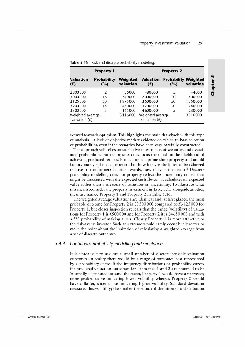
Property Investment Valuation 291
Ch
apte
r 5
skewed towards optimism. This highlights the main drawback with this type
of analysis – a lack of objective market evidence on which to base selection
of probabilities, even if the scenarios have been very carefully constructed.
The approach still relies on subjective assessments of scenarios and associ-
ated probabilities but the process does focus the mind on the likelihood of
achieving predicted returns. For example, a prime shop property and an old
factory may yield the same return but how likely is the latter to be achieved
relative to the former? In other words, how risky is the return? Discrete
probability modelling does not properly reflect the uncertainty or risk that
might be associated with the expected cash-flows – it calculates an expected
value rather than a measure of variation or uncertainty. To illustrate what
this means, consider the property investment in Table 5.15 alongside another,
these are named Property 1 and Property 2 in Table 5.16.
The weighted average valuations are identical and, at first glance, the most
probable outcome for Property 2 is £3 500 000 compared to £3 125 000 for
Property 1, but closer inspection reveals that the range (volatility) of valua-
tions for Property 1 is £500 000 and for Property 2 it is £4 680 000 and with
a 5% probability of making a loss! Clearly Property 1 is more attractive to
the risk-averse investor. Such an extreme would rarely occur but it serves to
make the point about the limitation of calculating a weighted average from
a set of discrete outcomes.
5.4.4 Continuous probability modelling and simulation
It is unrealistic to assume a small number of discrete possible valuation
outcomes. In reality there would be a range of outcomes best represented
by a probability curve. If the frequency distributions or probability curves
for predicted valuation outcomes for Properties 1 and 2 are assumed to be
‘normally distributed’ around the mean, Property 1 would have a narrower,
more peaked curve indicating lower volatility whereas Property 2 would
have a flatter, wider curve indicating higher volatility. Standard deviation
measures this volatility; the smaller the standard deviation of a distribution
Table 5.16 Risk and discrete probability modeling.
Property 1 Property 2
Valuation (£)
Probability (%)
Weighted valuation
Valuation (£)
Probability (%)
Weighted valuation
2 800 000 2 56 000 –80 000 5 –4 0003 000 000 18 540 000 2 000 000 20 400 0003 125 000 60 1 875 000 3 500 000 50 1 750 0003 200 000 15 480 000 3 700 000 20 740 0003 300 000 5 165 000 4 600 000 5 230 000Weighted average valuation (£)
3 116 000 Weighted average valuation (£)
3 116 000
Wyattp-05.indd 291Wyattp-05.indd 291 8/18/2007 12:10:40 PM8/18/2007 12:10:40 PM

292 Property Valuation
Ch
apter 5
the less volatile it is. See Appendix 5B (See Appendix 5B at www.blackwell-
publishing.com/wyatt) for a little refresher on measures of central tendency,
dispersion and probabilities.
Let’s assume that we have asked 50 valuers to value Properties 1 and 2 from
Section 5.4.2 and the mean valuation for Property 1 was £3 200 000 with a
standard deviation of £500 000 and for Property 2 the mean valuation was
£3 500 000 but with a much higher standard deviation of £1 000 000. The
‘coefficient of variation’ is a useful measure of volatility because it gives a
percentage variance for one standard deviation either side of the mean and is
useful for comparing projects whose expected values (means) are not equal.
It measures dispersion relative to the mean. The coefficient of variation for
Property 1 is 15.63% and for Property 2 it is 28.57%. Property 1 is less vola-
tile by both standard deviation and coefficient of variation measures.
So far we have looked at assigning probabilities to the valuation outcomes
but what about the values chosen for the key input variables? At the moment
they are point estimates but could they not take one of a possible range
of values with some more likely than others (Sayce et al., 2006)? Would
they not be better modelled as probability distributions? Now we enter a
whole world of concurrent probability distributions of variables that might
be correlated and our tiny little brains fail to cope with such complexity.
We need computer power to help in the form of a simulation programme.
Simulation enables valuers to assign probabilities to input variables in the
valuation and run simulations of most likely combinations of values of these
input variables in order to produce a probability distribution and associated
confidence range for the output valuation. Statistics that quantitatively sum-
marise the uncertainty surrounding the valuation output can then be calcu-
lated. Most notably these would include a mean valuation and a measure of
dispersion, usually the standard deviation.
Simulation involves a series of steps:
Build a valuation model and identify key variables. The valuation might be
constructed using an ARY or DCF technique and the best estimates of the
input variables are likely to be used when constructing the model. These
input variables can be classified as either deterministic variables, which can
be predicted with a high degree of certainty, or stochastic variables, which
cannot be predicted with a high degree of certainty. Generally the stochastic
variables that have a significant impact on the valuation are the ones on
which simulation is likely to be run. Deterministic variables might include
the rent review period, purchase and management costs. Key stochastic vari-
ables will include the ARY, MR, rental growth rate and exit yield. The TRR
is unlikely to vary. When looking at flexi-leases in particular it may be wise
to simulate different void periods and associated costs too.
Ascribe a range of probable values or probability distribution for each key input variable. The key variables need to be represented as a probabil-
ity distribution rather than a point estimate. A probability distribution is
a device for presenting the quantified risk for the variable. Ideally the
Wyattp-05.indd 292Wyattp-05.indd 292 8/18/2007 12:10:40 PM8/18/2007 12:10:40 PM

Property Investment Valuation 293
Ch
apte
r 5
estimation of probability distributions for key variables would be based on
empirical evidence but often the data are not available in a sufficient quan-
tity to allow this. A pragmatic alternative is to gather opinions of possible
values of each variable, along with their probability of occurrence, from
experts. These expert opinions could then be used to select an appropriate
probability function, of which there are many. The probability functions that
are typically chosen are the continuous ‘normal’ distribution (in which case
a mean and standard deviation would need to be specified) and the closed
‘triangular’ distribution (in which case the mode, minimum and maximum
values would need to be specified). A useful characteristic of the triangular
distribution is that, unlike the normal distribution, symmetry does not have
to be assumed; the maximum and minimum values do not have to be equally
spaced on each side of the mode. In this way the triangular distribution
might offer a more realistic representation than the normal distribution if
more upside or downside risk is expected.
The input variables may also be independent or dependent. An indepen-
dent variable is unaffected by any other variable in the model whereas a
dependent variable is determined in full or in part by one or more other
variables in the model. Different degrees of interdependence can significantly
affect the simulation result. It is therefore necessary to specify the extent to
which the input variables are correlated. Sayce et al. (2006) note that signifi-
cant research is needed in this area to establish an empirical base for correla-
tion assumptions, particularly, as Byrne (1996) points out, correlations may
be non-linear. This is especially pertinent in the case of development valua-
tion, which we will look at in the next chapter, because, unlike the valuation
of standing property investments, which typically involves a small number
of key variables, development valuation can incorporate a large number of
correlated input variables. McAllister (2001) points out that, in general, as
correlation reduces, the mean and standard deviation increase, but this is not
proportionate since the covariance also increases.
Run simulation. Having selected the key variables and their probability dis-
tributions the simulation can begin. Simulation refers to the method whereby
the distribution of valuation outcomes is generated by recalculating the
valuation model many times, each time using different randomly sampled
combinations of values from within the parameters of the probability distri-
butions of the key stochastic variables.4 In other words, because some values
of key variables will have a greater probability of being achieved than oth-
ers, the sample selection procedure ensures that these values are simulated
more frequently. This simulation process determines the range and probabil-
ity of the valuation outcome.
Output. When setting up the simulation program the uncertain output
variable in the valuation model would have been specified; invariably, this
will be the valuation figure. The simulation results will provide information
about the distribution of the output variable, including its central tendency
(mean, median, mode), spread (range, standard deviation) and measures of
Wyattp-05.indd 293Wyattp-05.indd 293 8/18/2007 12:10:40 PM8/18/2007 12:10:40 PM

294 Property Valuation
Ch
apter 5
symmetry (skewness) and peakedness (kurtosis). Regression analysis is also
undertaken to rank the input variables in terms of their impact on the output
valuation.
Let us look at two examples using the @RISK simulation software
add-in to Microsoft Excel. The first example is a short-cut DCF valuation
of a rack-rented freehold property investment recently let on conventional
lease terms. Our best estimates of the key variables are an ARY/exit yield
of 8%, a MR of £50 000 per annum and a rental growth rate of 2.5% per
annum. An ARY valuation would produce a capital value of £625 000 and,
assuming a TRR of 10%, a point estimate DCF valuation would generate a
figure of £628 593 – a higher figure because the explicit growth rate of 2.5%
was used instead of the rate of 2.33% implied by an ARY of 8% and a target
rate of 10%.
MR (£) 50 000YP 5 years @ 10% 3.7908
189 539Reversion to MR (£) 50 000Growth rate over 5 years @ 2.5% 1.1314
56 570YP in perpetuity @ 8% 12.5000PV £1 for initial term @ 10% 0.6209
439 054Valuation (£) 628 592
We are now going to introduce some uncertainty into three key variables
in the above valuation. The exit yield has a triangular distribution with a
mode of 8%, a minimum value of 6.5% and a maximum of 9%. Both the
MR and rental growth rate are normally distributed with a mean of £50 000
and standard deviation of £5000 in the case of the former and 2.5% and 1%
respectively for the latter. Correlations between these variables are subjec-
tively chosen and specified in Table 5.17.
The second example is an identical property but this time recently let on
flexi-lease terms that incorporate a break option at the end of year 5. If we
value this property using a short-cut DCF and assume a void of 1 year at
Table 5.17 Correlation matrix.
ARY/exit
yieldMarket
rentGrowth rate
(explicit)
ARY/exit yield 1Market rent –0.5 1Growth rate (explicit) –0.5 0.5 1
Wyattp-05.indd 294Wyattp-05.indd 294 8/18/2007 12:10:40 PM8/18/2007 12:10:40 PM

Property Investment Valuation 295
Ch
apte
r 5
the end of year 5 but keeping the values of all other variables the same, the
valuation would be as follows:
MR (£) 50 000YP 5 years @ 10% 3.7908
189 539Void for 1 yearReversion to MR (£) 50 000Growth rate over 6 years @ 2.5% 1.1597
57 985YP in perpetuity @ 8% 12.5000PV £1 for initial term plus void @ 10% 0.5645
409 135Valuation (£) 598 675
Clearly, uncertainty surrounds the exercise of the break option and so sim-
ulation can allow this uncertainty to be quantified by representing the length
of any void period that may occur after the end of year 5 as a probability
distribution, here based on a normal distribution with a mean of 1 year and
a standard deviation of 1 year.
Ten thousand iterations were run and the valuation outputs from the con-
ventional and flexi-leased properties are shown below. The optimistic skew
of the exit yield distribution has increased the mean valuation of both proper-
ties approximately £15 000 above the original point estimates. In both cases
the standard deviation around the mean was just under £100 000. Figure 5.5
and the skewness value in Table 5.18 reveal that both output distributions
are positively skewed, the property let under standard lease terms slightly
more so. This is because the exit yield, which is itself positively skewed,
explains more of the variation in value of the standard let investment, as
shown in Table 5.19.
The ‘regression’ columns in Table 5.19 report standardised regression (β)
coefficients for the input variables. A coefficient of 0 indicated no significant
relationship between the input and the valuation while a coefficient of +1 or
4.54
3.53
2.52
1.51
0.500.3 0.5 0.7 0.9 1.1 0.3 0.5 0.8 1.1
x ≤ 494,217.945%
x ≤ 815,932.8895%
x ≤ 460,019.095%
x ≤ 786,519.8195%
Values in millions
Val
ue in
10–6
4.54
3.53
2.52
1.51
0.50
Val
ue in
10–6
Mean = 643681.6
Values in millions
Mean = 614229.6
(a) (b)
Figure 5.5 Valuation probability distributions: (a) distribution for valuation of standard lease and (b) distribution for valuation of fl exi-lease.
Wyattp-05.indd 295Wyattp-05.indd 295 8/18/2007 12:10:41 PM8/18/2007 12:10:41 PM

296 Property Valuation
Ch
apter 5
–1 indicates a +1 or –1 change in the standard deviation of the valuation for
a +1 or –1 change in the standard deviation of the input. The ‘correlation’
columns report Spearman’s rank-order correlation coefficient which can also
vary between –1 and +1. These two extremes would indicate a perfectly neg-
ative and a perfectly positive correlation respectively whereas a coefficient
of 0 indicates no correlation at all. It is important to examine the signs of the
coefficients to be sure that the correlation is in the right direction. If the R2
value reported by the regression results is high the relationship between the
input and output variables is linear. If the R2 value is low the relationship is
non-linear and rank-order correlation should be analysed to determine the
sensitivity of the model. Remember, though, that this is an illustration and,
because of the lack of evidence to support the correlations between the input
variables, it should not be regarded as a practical application.
5.4.5 Arbitrage
Simulation techniques allow the impact of uncertainty surrounding key input
variables to be examined. One variable was not considered to be uncertain,
however, and this was the TRR. The assumption was that the investor would
know what this was and would stick to it. But what if the target rate is not
set in stone over the holding period for the investment? Different portions of
forecast cash-flows – the rent agreed for the first 5 years and the rent agreed
at the first rent review for example – may have different levels of risk and
therefore different target rates (Appraisal Institute, 2001). To consider the
valuation implications of this we can use an option pricing technique known
as arbitrage.6
Table 5.18 Summary statistics.
Standard
lease Flexi-lease
Mean (£) 643 682 614 230Std Dev (£) 98 214 99 581Skewness 0.3573 0.3134Kurtosis 3.1323 3.1511
Table 5.19 Sensitivity.
Standard lease Flexi-lease
Regression Correlation Regression Correlation
Market rent 0.651 0.918 0.612 0.875Exit yield –0.314 –0.737 –0.290 –0.710Growth rate (explicit)
0.224 0.686 –0.265 –0.220
Void period — — 0.247 0.681
Wyattp-05.indd 296Wyattp-05.indd 296 8/18/2007 12:10:41 PM8/18/2007 12:10:41 PM

Property Investment Valuation 297
Ch
apte
r 5
The arbitrage valuation technique was first applied to property invest-
ment by French and Ward (1995) and is based on the premise that each
part of a cash-flow from any investment should be valued by comparing
it with other assets with similar risk characteristics (Havard, 2000): think
of how you might ‘lay off’ a bet. Like the short-cut DCF valuation tech-
nique, when applied to property, the arbitrage valuation technique adopts a
term and reversion approach. But, instead of using a yield based on property
risk factors to capitalise the term income, the arbitrage approach uses a low
discount rate that is based on tenant risk factors. In other words the term
income is regarded as comparable to income from an illiquid bond based on
the tenant’s default risk. The value at reversion is based upon the capitalisa-
tion of the rent at an ARY, representing a notional sale at this point. The
arbitrage technique differs from the short-cut DCF technique in its approach
to the deferral of this notional sale value and the rental value on which it is
determined.
The short-cut DCF technique uses a constant (average) growth rate to
project the MR at the review date and a single target rate to discount all
cash-flows, and this can distort the risk profile into the future by putting less
relative weight on distant cash-flows (Crosby, 1996). The arbitrage approach
questions the appropriateness of using a single target rate and suggests that
it should be based on debt and equity components of the financing package
used to purchase the investment. French and Ward (1995) derive two target
rates that can be used to discount the term and reversion components of a
reversionary property investment. Two rates are justified on the basis that
the term income is known and therefore certain, whereas future reversions
must be estimated. From the tenant’s viewpoint the term rent is certain over
the initial term and so the financial liability is equivalent to interest pay-
ments on any fixed income loan and can therefore be valued using a discount
rate appropriate for such payments. From the landlord’s viewpoint an addi-
tional risk premium might be appropriate to reflect illiquidity and tenant
default risk.
Consider a rack-rented freehold property investment let at £100 000 per
annum and for which the ARY is 8%. From the tenant’s perspective there is a
contractual obligation to pay £100 000 per annum rent for the first 5 years.
If the bank lending rate is 10% per annum, then
£100 000 × YP 5 years @ 10% = £379 079.
In valuing the second term the tenant is not certain of the rent in 5 years’
time but needs to estimate the amount that should be invested now to pro-
vide funds to offset the rent liability when known. Arbitrage principles sug-
gest that the tenant should find an asset with the same risk characteristics as
the rent liability and then value the second term by investing in that asset at
today’s price. The arbitrage investment is to invest in a similar freehold and,
to match the liability of the second 5-year term, the tenant would notion-
ally invest in the proportion of the freehold which would provide the first
5 years of rent, that is, £379 079/£1 250 0007 or 30.326% of the value of the
freehold. This notional investment is ‘held’ for 5 years and then ‘sold’.
Wyattp-05.indd 297Wyattp-05.indd 297 8/18/2007 12:10:42 PM8/18/2007 12:10:42 PM

298 Property Valuation
Ch
apter 5
Whatever the value of the freehold the sum realised will, assuming constant
yields and rates, be sufficient to offset the financial liability of the second term.
So if the tenant owns 30.326% of the freehold he would receive 30.326% of
the rent each year, that is, £30 326 per annum which, when capitalised for 5
years at 10%, equals £114 961. The total cost of the investment is therefore
£379 079 - £114 961 = £264 118. This process can be repeated to value sub-
sequent terms but if, as French and Ward (1996) suggest, we assume that the
arbitrage valuation must equal a more conventional valuation then we can
use the following formula to derive a reversion rate known as the ‘deferred
capital yield’ (DCY) either by iteration or by formula.
By iteration. A conventional ARY valuation of the property, assuming an
ARY of 8% and a MR of £100 000 per annum, would produce a capital
value of £1 250 000. This valuation needs to be broken down to differenti-
ate the target rates used to capitalise the known and unknown cash-flows.
As before, assume a discount rate of 10% for the known rent over the first
5 years. Knowing the capital value of the cash-flow over the first 5 years
(£379 080), the overall valuation (£1 250 000) and that the rent on reversion
will be capitalised into perpetuity at ARY of 8%, it is possible to calculate
the appropriate DCY by iteration (Havard, 2000).
Term (£) 100 000YP 5 years @ 10% 3.7908
379 080Reversion (£) 100 000YP perpetuity @ 8% 12.5000PV £1 5 years @ 7.49%a 0.6967
870 920Valuation (£) 1 250 000[a] Rate obtained by iteration
By formula.
11- ◊YP terma f,( )r r
1+ DCY=Term
[5.13]
where Term = period to revision
ra = ARY
rt = low-risk TRR
Substituting the values as above into Equation 5.11 the DCY is 7.49%
(French and Ward, 1996).
To recap, the arbitrage valuation technique is based on the assumption
that the value of the whole is equal to the sum of the term and reversion
Wyattp-05.indd 298Wyattp-05.indd 298 8/18/2007 12:10:42 PM8/18/2007 12:10:42 PM

Property Investment Valuation 299
Ch
apte
r 5
components. The capital value of the unknown rent after the first review is
calculated by capitalising the term rent using a low-risk yield and deducting
this from the total capital value of the subject property or a comparable. The
resultant reversionary value can be analysed for the DCY. An arbitrage valu-
ation thus proceeds as follows:
ÊËÁ
ˆ¯̃
È
ÎÍ
˘
˚˙+
È
ÎÍ
˘
˚˙
MR
PV = (CR ¥ YP for term) + (MR ¥ YP in perpetuity ¥ PV for term)
1- (1+ rt)-n
ra (1+ DCY)nrt
= CR ¥
[5.14]
where CR = contract rent for term
MR = Market rent
rt = TRR
n = period to next rent revision
French and Ward (1996) show how the arbitrage method can also be
applied to the valuation of reversionary property investments. A comparable
(but this time reversionary) freehold property investment let one year ago at
£80 000 per annum has been valued using a short-cut DCF technique. The
target rate is 12% and the ARY is 8%, giving an implied rental growth rate
of 4.63% per annum.
Term rent (£) 80 000YP 4 years @ 10% 3.1699
253 590Reversion to MR 100 000PV 4 years @ 7.494% 0.7490YP perpetuity @ 8% 12.5000
936 190Valuation (£) 1 189 780
However, the DCF approach still fails to recognise the different risk profiles
of the known and unknown cash-flows. Using the DCY calculated above for
the rack-rented comparable, the arbitrage valuation is
Term rent (£) 80 000YP 4 years @ 12% 3.0373
242 984Reversion to MR 100 000Growth @ (1.0463)^4 1.1985PV 4 years @ 12% 0.6355YP perpetuity @ 8% 12.5000
952 058Valuation (£) 1 195 042
Wyattp-05.indd 299Wyattp-05.indd 299 8/18/2007 12:10:42 PM8/18/2007 12:10:42 PM

300 Property Valuation
Ch
apter 5
This is a growth-implicit arbitrage valuation. A growth-explicit arbitrage
valuation can be produced by inflating the DCY at the implied rental growth
rate g (4.63%) to produce a capital yield (CY) as follows:
(1 + CY) = (1 + DCY) × (1 + g) [5.15](1 + CY) = 1.07494 × 1.0463CY = 12.47%And the valuation would be as follows:
Term (£) 80 000YP 4 years @ 10% 3.1699
253 590Reversion (£) 100 000Growth @ 4.63% pa 1.1985YP perpetuity @ 8% 12.5000PV £1 4 years @ 12.47% 0.6250
936 328Valuation (£) 1 189 918
Table 5.20 compares full growth-explicit DCF valuations of the rever-
sionary property investment assuming (1) target rates based upon arbitrage
principles and (2) a constant TRR.
Table 5.20 Growth-explicit DCF and arbitrage valuations.
(1) Arbitrage (2) DCF
Year Rent (£)a YP PV (£) YP @ 12% PV (£)
0–3 80 000 4 years @ 10% = 3.1699
253 589 4 years @ 12% = 3.0373
242 987
4–8 119 859 5 years @ 10% discounted @ 12.47% for 4 years = 2.3687
283 912 5 years @ 12% discounted @ 12% for 4 years = 2.2909
274 584
9–13 150 316 5 years @ 10% discounted @ 12.47% for 9 years = 1.3159
197 812 5 years @ 12% discounted @ 12% for 9 years = 1.300
195 399
14–18 188 514 5 years @ 10% discounted @ 12.47% for 14 years = 0.7310
137 823 5 years @ 12% discounted @ 12% for 14 years = 0.7376
139 049
19–23 236 418 5 years @ 10% discounted @ 12.47% for 19 years = 0.4061
96 026 5 years @ 12% discounted @ 12% for 19 years = 0.4185
98 950
24–perp 296 495 Perp @ 8% discounted @ 12.47% for 24 years = 0.7441
220 629 Perp @ 12% discounted @ 12% for 24 years = 0.8235
244 163
Valuation (£)
1 189 791 1 195 132
aGrowing at 4.63% per annum.Source: French and Ward (1995).
Wyattp-05.indd 300Wyattp-05.indd 300 8/18/2007 12:10:43 PM8/18/2007 12:10:43 PM

Property Investment Valuation 301
Ch
apte
r 5
Although the valuations are roughly the same, the values of each term
differ. The arbitrage value for the first term is higher because the income is
discounted at the low-risk yield of 10% rather than the uniform target rate
of 12%. Then, in the arbitrage approach, subsequent terms are discounted
at 12.47% rather than 12%. It could be argued that if the rent passing was
significantly below MR the discount rate applied to the term could be even
lower to reflect the reduced risk of tenant default. The arbitrage approach
thus requires consideration of the risk profile of the term and reversion
incomes. When valuing rack-rented freeholds both approaches will produce
the same answers.
The arbitrage method of property valuation has not been widely adopted
in practice. The selection of an appropriate target rate for the known ini-
tial term rent is subjective (French and Ward, 1996) and the technique still
requires good comparable evidence, although not so much if the period to
reversion is long and therefore a significant part of the rental value is capi-
talised at a bond rate (Havard, 2000). Simulation and arbitrage valuation
techniques push the boundaries of market data analysis to the limits. That
is no reason to dismiss them; rather it should act as a spur to the continued
improvement of property data so that these techniques may be developed
and refined.
Key points
Valuation variance has been identified in empirical studies of valuation prac-tice. The courts accept that a degree of variance is inevitable through the adoption of the margin of error principle. To an extent, because of the expert witness process in the courts, it is axiomatic that valuers also accept the existence of valuation variance. Indeed, Crosby et al. (1998) state that the margin of error principle was conceived by expert witnesses who are, by definition, experienced valuers.
A valuation accuracy of 100% is an unattainable goal. Annual research funded by the RICS helps quantify the extent of valuation inaccuracy and demonstrates a degree of openness that is to be applauded. Only by learn-ing more about the nature and extent of valuation inaccuracy, can methods to deal with valuation uncertainty be developed.
Simulation is a logical extension of sensitivity analysis, scenario testing and discrete probability modelling that adds a quantitative measure of risk to a single point estimate of value. It does this by assigning probability distribu-tions to key input variables. The drawback with this type of analysis at the moment is the lack of evidence on which to base these distributions and any correlations between them. Nevertheless, the discipline of building a ‘risk aware’ simulation model can lead to a deeper understanding of the nature of the property investment under consideration.
Short-cut DCF and arbitrage approaches go some way to assigning the cor-rect value of to various parts of the cash-flow but do not address the issue of volatility of future cash-flows.
Wyattp-05.indd 301Wyattp-05.indd 301 8/18/2007 12:10:44 PM8/18/2007 12:10:44 PM

302 Property Valuation
Ch
apter 5
Notes
1. Ordinary least squares but this time regressing price on value, normalising for
size by using price or value per unit area as last time but, unlike Brown, using
these in their untransformed state rather than taking logs.
2. When using statistical techniques such as ordinary least squares regression a
number of assumptions are typically made. One of these is that the error term
has a constant variance. This will be true if the observations of the error term are
assumed to be drawn from identical distributions. Heteroskedasticity is a viola-
tion of this assumption.
3. The valuations were adjusted for market movement between the valuation date
and sale agreement date by increasing or decreasing the valuation according
to movements in the IPD capital growth index for the relevant market sector.
Percentage difference between valuation and sale price was found by applying
the following formula: Difference = (price – adjusted valuation)/price.
4. Havard (2000) provides a useful illustration of how this process works in the
case of two variables; annual rental growth rate and exit yield to which discrete
probabilities have been assigned. The simulation programme randomly selects
from the cumulative probability distribution for each variable. If we assume 22
was randomly selected for rental growth and 67 for the exit yield this would
equate to 3% rental growth rate and an exit yield of 9.25%. These sample values
are then input into an iteration of the valuation model.
5. Rank-order correlation calculates the relationship between two data sets by
comparing the rank of each value in a data set. To calculate rank, the data are
sorted from lowest to highest and assigned numbers (ranks) that correspond to
their position in the order.
6. Arbitrage refers to the activity of market traders who compare the prices of simi-
lar assets, selling or buying to realise profits if the prices are out of line with one
another. The principle is best known in foreign exchange markets.
7. Market rent of £100 000 per annum capitalised at an assumed freehold ARY
of 8%.
References
Appraisal Institute (2001) The Appraisal of Real Estate, 12th Edn, The Appraisal
Institute, Chicago, IL’ USA.
Baum, A. (2000) Commercial Real Estate Investment, Chandos, Oxford, UK.
Baum, A. and Crosby, N. (1995) Property Investment Appraisal, 2nd edn, Routledge,
London, UK.
Bretten, J. and Wyatt, P. (2001) Variance in commercial property valuations: an
empirical study, Journal of Property Investment and Finance, 19, 3, 267–282.
Brown, G. (1985) Property investment and performance measurement: A reply,
Journal of Valuation, 4, 1, 33–44.
Brown, G. and Matysiak, G. (2000) Real Estate Investment: A Capital Market Approach, FT Prentice Hall, Harlow, Essex, UK.
Byrne, P. (1996) Risk, Uncertainty and Decision-making in Property Development, 2nd edn; E. and F. N. Spon, London, UK.
Crosby, N. (1990) The practice of property investment appraisal: reversionary free-
holds in the UK, Journal of Property Valuation and Investment, 9, 109–122.
Wyattp-05.indd 302Wyattp-05.indd 302 8/18/2007 12:10:44 PM8/18/2007 12:10:44 PM

Property Investment Valuation 303
Ch
apte
r 5
Crosby, N. (1991) Over-rented freehold property valuations, Journal of Property Valuation and Investment, 10, 517–524.
Crosby, N. (1996) Valuation and arbitrage: a comment, Journal of Property Research,
13, 211–220.
Crosby, N., Lavers, A. and Murdoch, J. (1998) Property valuation variation and the
‘margin of error’ in the UK, Journal of Property Research, 15, 4, 305–330.
Crosby, N. and Goodchild, R. (1992) Reversionary freeholds: problems with over-
renting, Journal of Property Valuation and Investment, 11, 67–81.
Crosby, N. and Murdoch, S. (1994) Capital valuation implications of rent-free peri-
ods, Journal of Property Valuation and Investment, 12, 2, 51–64.
Fraser, W. (1993) Principles of Property Investment and Pricing, 2nd edn, Macmillan,
Basingstoke, Hampshire, UK.
French, N. (2001) Uncertainty in property valuation: the pricing of flexible leases,
Journal of Corporate Real Estate, 3, 1, 17–27.
French, N. and Mallinson, M. (2000) Uncertainty in property valuation, Journal of Property Investment and Finance, 18, 1, 13–32.
French, N. and Ward, C. (1995) Valuation and arbitrage, Journal of Property Research, 12, 1–11.
French, N. and Ward, C. (1996) Applications of the arbitrage method of valuation,
Journal of Property Research, 13, 47–56.
Gallimore, P. (1994) Aspects of information processing in valuation judgement and
choice, Journal of Property Research, 11, 2, 97–110.
Gallimore, P. and Wolverton, M. (1997) Price-knowledge-induced bias: A cross-
cultural comparison, Journal of Property Valuation and Investment, 15, 3,
261–273.
Hagar, D. and Lord, D. (1985) The property market, property valuations and prop-
erty performance measurement, Journal of the Institute of Actuaries, (112, Part, 1),
No 450, 19–60.
Havard, T. (2000) Investment Property Valuation Today, Estates Gazette,
London, UK.
Hutchison, H., MacGregor, B., Nanthakumaran, N., Adair, A. and McGreal, S. (1996)
Variations in the Capital Valuations of UK Commercial Property, Research Report,
Royal Institution of Chartered Surveyors, London, UK.
Kinnard, W., Lenk, M. and Worzala, E. (1997) Client pressure in the commer-
cial appraisal industry: how prevalent is it? Journal of Property Valuation and Investment, 15, 3, 233–244.
IPD/Drivers Jonas (1988) The Variance in Valuations, Drivers Jonas, London, UK.
IPD/Drivers Jonas (1990) The Variance in Valuations: 1990 Update, Drivers Jonas,
London, UK.
IPF (2005) Understanding Commercial Property Investment: A Guide for Financial Advisers, 2005 Edition, Investment Property Forum, London, UK.
IVSC (2005) International Valuation Standards, 7th edn. International Valuation
Standards Committee, London, UK.
Lavers, A., Williams, M., Crosby, N. and Foster, H. (1996) Commercial Property Loan Valuations: Liability, Process and Changes, Cutting Edge Conference, Royal
Institution of Chartered Surveyors, London, UK.
Lizieri, C. and Venmore-Rowland, P. (1991) Valuation accuracy: a contribution to
the debate, Journal of Property Research, 8, 115–122.
Martin, D. (1991) Valuation: over-rented property, Estates Gazette, December 7, 52
McAllister, P. (2001) Pricing short leases and break clauses using simulation method-
ology, Journal of Property Investment and Finance, 19, 4, 361–374.
Wyattp-05.indd 303Wyattp-05.indd 303 8/18/2007 12:10:44 PM8/18/2007 12:10:44 PM

304 Property Valuation
Ch
apter 5
McAllister, P. and O’Roarty, B. (1999) Pricing Break Clauses: a Fundamental
Approach, Proceedings of the RICS ‘Cutting Edge’ Property Research Conference,
Royal Institution of Chartered Surveyors, London, UK.
RICS (2002) The Carsberg Report on Property Valuations, Royal Institution of
Chartered Surveyors, London, UK.
RICS (2003) RICS Appraisal and Valuation Standards, 5th edn. (as amended), Royal
Institution of Chartered Surveyors, RICS Business Services Ltd, Coventry, UK.
RICS (2005) Valuation and Sale Price, 2005 report, Royal Institution of Chartered
Surveyors, London, UK.
Sayce, S., Smith, J., Cooper, R. and Venmore-Rowland, P. (2006) Real Estate Appraisal:from Value to Worth, Blackwell Publishers, Oxford, UK.
Sykes, S. (1981) Property Valuations: a rational model, The Investment Analyst, 61, 20–26.
Syms, P. (1996) Contaminated land and other forms of environmental impairment:
an approach to valuation, Journal of Property Valuation and Investment, 14, 2.
Ward, C. and French, N. (1997) The valuation of upward-only rent reviews: an option
pricing model, Journal of Property Valuation and Investment, 15, 2, 171–182.
Wyattp-05.indd 304Wyattp-05.indd 304 8/18/2007 12:10:44 PM8/18/2007 12:10:44 PM