chapter 5 - the q-tensor model with uniaxial constraint
TRANSCRIPT

Chapter 5
The Q-tensor model withuniaxial constraintJuan Pablo Borthagaraya,b,d and Shawn W. Walkerc,∗,e
aDepartment of Mathematics, University of Maryland, College Park, MD, United States,bDepartamento de Matemática y Estadística del Litoral, Universidad de la República, Salto,Uruguay, cDepartment of Mathematics and Center for Computation and Technology (CCT),Louisiana State University, Baton Rouge, LA, United States∗Corresponding author: e-mail address: [email protected]
Contents1 Physics of liquid crystals 314
1.1 Fundamentals 3141.2 Applications 316
2 Modeling of nematic liquid crystals 3162.1 Order parameters 3162.2 Continuum mechanics 3192.3 Dynamics 324
3 Mathematical formulation 3253.1 Oseen-Frank 3253.2 Landau-de Gennes 3263.3 Ericksen 331
4 The uniaxially constrained Q-model 3444.1 Modeling assumptions 3454.2 Discretization 347
4.3 Gradient flow 3494.4 Gamma convergence 3544.5 Numerical experiment 357
5 Colloidal effects 3605.1 Conforming non-obtuse mesh 3615.2 Immersed boundary method 364
6 Electric fields 3706.1 Modified energies 3716.2 Computational electric field
example 3737 The Landau-de Gennes model with
and without the uniaxial constraint 3738 Conclusion 376References 377
AbstractThis chapter is about the modeling of nematic liquid crystals (LCs) and their numericalsimulation. We begin with an overview of the basic physics of LCs and discuss some oftheir many applications. Next, we delve into the modeling arguments needed to obtainmacroscopic order parameters which can be used to formulate a continuum model. Wethen survey different continuum descriptions, namely the Oseen-Frank, Ericksen, andLandau-de Gennes (Q-tensor) models, which essentially model the LC material like ananisotropic elastic material. In particular, we review the mathematical theory underlyingthe three different continuum models and highlight the different trade-offs of using thesemodels.
d. JPB has been supported in part by NSF grant DMS-1411808.e. SWW has been supported in part by NSF grant DMS-1555222 (CAREER).
Handbook of Numerical Analysis, Volume 22, ISSN 1570-8659, https://doi.org/10.1016/bs.hna.2020.09.001Copyright © 2021 Elsevier B.V. All rights reserved.
313

314 Handbook of Numerical Analysis
Next, we consider the numerical simulation of these models with a survey of variousmethods, with a focus on the Ericksen model. We then show how techniques fromthe Ericksen model can be combined with the Landau-de Gennes model to yield aQ-tensor model that exactly enforces uniaxiality, which is relevant for modeling manynematic LC systems. This is followed by an in-depth numerical analysis, using toolsfrom �-convergence, to justify our discrete method. We also show several numericalexperiments and comparisons with the standard Landau-de Gennes model.
KeywordsNematic liquid crystals, Finite element method, Gamma-convergence, Landau-de Gennes,Defects
MSC Codes65N30, 49M25, 35J70
1 Physics of liquid crystals
1.1 Fundamentals
The name “liquid crystal” appears self-contradictory. A crystal has a rigidmolecular structure and so is associated with being a solid. How could a crystalbe liquid? Thinking more broadly, a crystal is matter that possesses some kindof macroscopic order, such as having individual molecules arranged in a lattice.On the other hand, a liquid has no macroscopic order.
Liquid crystals (LCs) are a meso-phase of matter, having a degree of macro-scopic order that is between a liquid and a solid (Virga, 1994). A classic solidcrystal has both translational order (points in the lattice do not move) and ori-entational order (neighboring molecules have similar orientation). A LC has nostrong translational order, i.e. the molecules are free to slide about, but they mustroughly maintain the same orientation with neighboring molecules. Thus, LCshave partial orientational order.
The initial, accidental discovery of LCs is classically attributed to the Aus-trian botanist Friedrich Reinitzer (Reinitzer, 1888, 1989), who was studyingcarrots. While heating cholesteryl benzoate, he saw the material exhibit an LCphase. In order to better understand this, he sought the help of German physicist,Otto Lehmann (Lehmann, 1889) who had experimental apparatus capable ofbetter analysis. After this initial work, Lehmann continued to study LCs, whileReinitzer moved on. Further information on the history of LCs can be found inSluckin et al. (2004), which contains translations of Reinitzer’s and Lehmann’sinitial papers. Moreover, one can consult (de Gennes and Prost, 1995; de Jeu,2012; Luckhurst and Veracini, 1994; Mottram and Newton, 2014) for more de-tails on the basic physics of LCs.
The LC state may be obtained as a function of temperature between thecrystalline and isotropic liquid phases; in such a case, the material is calleda thermotropic LC. Other classes include lyotropic and metallotropic LCs, in

The Q-tensor model with uniaxial constraint Chapter | 5 315
which concentration of the LC molecules in a solvent or the ratio between or-ganic and inorganic molecules determine the phase transitions, respectively.
Let us consider thermotropic LCs. In a crystalline solid, molecules exhibitboth long-range ordering of the positions of the centers and orientation of themolecules. As the substance is heated, the molecules gain kinetic energy andlarge molecular vibrations usually make these two ordering types disappear.This results in a fluid phase. In substances capable of producing an LC meso-phase, the long-range orientational ordering survives until a higher temperaturethan the long-range positional ordering. Whenever long-range positional order-ing is completely absent, but orientational order remains, the LC is regardedas nematic. At lower temperatures, the molecules may order along a preferreddirection, forming layered structures: this is called the smectic phase. In turn,smectic mesophases may be classified into subclasses (such as smectics A,smectics C and hexatic smectics), depending on the type and degree of posi-tional and orientational order (de Gennes and Prost, 1995). Some substanceswith chiral molecules (i.e. different from their mirror image) may give rise to acholesteric mesophase, in which the structure possesses a helical distortion.
This chapter will only consider nematic LCs, and regard their molecules asrods, elongated in one direction and thin in the other two directions. Imagininga bunch of thin rods packed together, it is natural to expect the orientation ofneighboring rods to be similar, but the rods are free to slide along each other.Indeed, the partial order of LCs is essentially due to the anisotropic shape of theLC molecules. Naturally, most LC molecules do not possess axial symmetry.If the molecules resemble more laths than rods, it is expected that the energyinteraction can be minimized if the molecules are fully aligned; this necessarilyinvolves a certain degree of biaxiality. Roughly, this was the rationale behindthe prediction of the biaxial nematic phase by Freiser (1970).
Since that seminal work, empirical evidence of biaxial states in certain ly-otropic LCs has been well documented (see Yu and Saupe, 1980, for example).Nevertheless, for thermotropic LCs the nematic biaxial phase remained elusivefor a long period, and was first reported long after Freiser’s original prediction(Acharya et al., 2004; Madsen et al., 2004; Prasad et al., 2005). As pointed outby Sonnet and Virga (2012, Section 4.1),
The vast majority of nematic liquid crystals do not, at least in homogeneousequilibrium states, show any sign of biaxiality.
Therefore, in this chapter, we shall focus mainly on uniaxial LCs. We discussthree models for the equilibrium configurations. Uniaxiality is naturally builtinto both the Oseen-Frank and the Ericksen models, as the LC orientation ismodeled by a vector field. In contrast, the Landau-de Gennes model representsmolecular orientation by means of a tensor field, and thus accounts for biaxiality.However, one can enforce uniaxiality and obtain a model that is not equivalentto either the Ericksen or the Oseen-Frank models. In particular, the uniaxially

316 Handbook of Numerical Analysis
constrained Landau-de Gennes model represents the LC molecule orientation bya line field, and thus it allows for non-orientable configurations. We will discussthis with more detail in Section 4.
1.2 Applications
The most well-known application of LCs is in electronic displays (Hoogboomet al., 2007; Roques-Carmes et al., 2004), which is due to an LC’s birefringenceproperty. Indeed, some LC materials polarize light (depending on the orientationof molecules) and this can be controlled through external fields, such as electricfields. This, combined with sophisticated engineering, delivers the flat panel LCdisplay.
However, many newer uses for LCs are being found in material science, thateither further build on LCs ability to manipulate light or take advantage of themechanical properties of the material’s anisotropy (Lagerwall and Scalia, 2012).For example, Humar and Muševic (2010) demonstrates three dimensional LCdroplets that act as lasers, which may be used as bio-sensors. Self-assemblyof rigid particles (inclusions) immersed in an LC medium (Copar et al., 2014,2015) has the potential to make new materials. Clever optical effects with LCdroplets (Schwartz et al., 2018) provide novel means of creating secure “mark-ers” that cannot be counterfeit.
Furthermore, LC models provide a test bed for investigating continuum mod-els of complex fluids (e.g. Ericksen-Leslie (Cruz et al., 2013; Mottram et al.,2013; Walkington, 2011)), especially swarms of bacteria (Vicsek and Zafeiris,2012; Marchetti et al., 2013; Giomi, 2015) which is sometimes called activematter (Ramaswamy, 2010, 2017; Doostmohammadi et al., 2018; Miles et al.,2019). The shape of a bacterium is very reminiscent of LC molecules (elongatedrods) so it is not surprising that LC models, coupled with fluid dynamics, maybe reused. Therefore, LC research is a very active field within physics, mathe-matics, biology, and soft-matter in general.
2 Modeling of nematic liquid crystals
We review three models for the equilibrium states of LCs. Specifically, weshow how to obtain a continuum description by an appropriate averaging overmolecules. This leads to continuum mechanics type models that derive fromminimizing an energy; we refer to de Gennes and Prost (1995), Virga (1994),Mottram and Newton (2014) for more details on the modeling of LCs.
2.1 Order parameters
Modeling individual LC molecules is certainly viable via molecular dynamics orMonte Carlo methods (Biscarini et al., 1995; Vanzo et al., 2012; Moreno-Razoet al., 2012; Whitmer et al., 2013; Teixeira-Souza et al., 2015; Changizrezaeiand Denniston, 2017) and has the advantage of being based on first principles

The Q-tensor model with uniaxial constraint Chapter | 5 317
(i.e. completely “correct”), but is also very expensive computationally. In orderto build on these models for, say, coupling to fluids or doing optimal design,we require a macroscopic description of LCs. Usually, the transition betweenphases of different symmetry is described in terms of an order parameter, thatrepresents the extent to which the configuration of the more symmetric phasediffers from that of the less symmetric phase.
In the following discussion, we fix the spatial dimension to be d = 3. As afirst step, suppose we have an ensemble of LC molecules in a small region wherethe state of each molecule is defined by its orientation in R3, i.e. let p ∈ S2 bea vector in the unit sphere that indicates the orientation of an LC molecule.Let ρ(p) ≥ 0 be the probability distribution of the orientation of LC molecules.Obviously, the distribution of LC molecules may vary in space (and in time), e.g.ρ ≡ ρ(x,p), but we shall omit the dependence on these variables for simplicityof notation. It is reasonable to assume that an LC molecule is just as likely to beobserved with orientation p as −p; hence, ρ satisfies ρ(p) = ρ(−p). Based onthis head-to-tail symmetry, it must be that∫
S2pρ(p) dp = 0, (1)
so direct averaging does not yield a useful order parameter.Therefore, the first nontrivial information on the molecule distribution is
given by the second moments of ρ, namely:∫S2
ppT ρ(p) dp = M, (2)
where M ∈ R3×3 is symmetric and effectively captures the average state ofthe LC molecules (i.e. this is a useful order parameter). For a uniformly ran-dom (isotropic) distribution of LC molecules, ρ(p) = 1/(4π) and M = Miso =(1/3)I. Thus, it is convenient to define an auxiliary matrix
Q := M − Miso, (3)
which is symmetric and traceless, i.e.
Q ∈ � :={
Q ∈R3×3 | Q = QT , tr Q = 0}
. (4)
Clearly, for an isotropic distribution of LC molecules, Q = 0. However, aspointed out in Virga (1994, Sec. 1.3.4), Q = 0 is a necessary but not sufficientcondition for isotropy. For the sake of obtaining a continuum theory in whichmicroscopic order is described by Q only, we shall regard all distributions satis-fying Q = 0 as isotropic.
We can further characterize Q by its eigenframe and is often written in theform:
Q = s1(n1 ⊗ n1) + s2(n2 ⊗ n2) − 1
3(s1 + s2)I, (5)

318 Handbook of Numerical Analysis
where n1, n2 are orthonormal eigenvectors of Q, with eigenvalues given by
λ1 = 2s1 − s2
3, λ2 = 2s2 − s1
3, λ3 = − s1 + s2
3, (6)
where λ3 corresponds to the eigenvector n3 ⊥ n1,n2. The eigenvalues of Q areconstrained by
−1
3≤ λi =
∫S2
(p · ni )2ρ(p) dp − 1
3≤ 2
3, i = 1,2,3. (7)
When all eigenvalues are equal, since Q is traceless, we must have λ1 = λ2 =λ3 = 0 and s1 = s2 = 0, i.e. the distribution of LC molecules is isotropic. If twoeigenvalues are equal, i.e.
λ1 = λ2 ⇔ s1 = s2,
λ1 = λ3 ⇔ s1 = 0,
λ2 = λ3 ⇔ s2 = 0,
(8)
then we encounter a uniaxial state, in which either molecules prefer to orient inalignment with the simple eigenspace (in case it corresponds to a positive eigen-value) or perpendicular to it (in case it corresponds to a negative eigenvalue). Ifall three eigenvalues are distinct, then the state is called biaxial. We recall that,as discussed in Section 1.1, most nematic LCs can be effectively modeled asuniaxial states.
Let us consider a uniaxial state for Q, that can be written in the equivalentform
Q = s
(n ⊗ n − 1
3I)
. (9)
Above, n is the main eigenvector with eigenvalue λ = 2s/3; the other two eigen-values equal −s/3. The scalar field s is called the degree of orientation of theLC molecules. Taking into account identity (6) and the restriction (7), it followsthat the physically meaningful range is s ∈ [−1/2,1]. As Fig. 1 illustrates, the s
variable characterizes the local order. In case s = 1, the molecular long axes arein perfect alignment with the direction of n, whereas s = −1/2 represents thestate in which all molecules are perpendicular to n.
Remark 1 (Problems in 2d). The discussion above simplifies considerablywhen d = 2. Indeed, the fact that Q is a zero-trace tensor forces it to be uniaxial.Writing Q as (9), we deduce that its eigenvalues are λ1 = s/2, with eigenvec-tor n, and λ2 = −λ1, with eigenvector n⊥. Because eigenvalues are constrainedto satisfy λi ∈ (−1/2,1/2), we deduce that the physically meaningful range iss ∈ (−1,1). Actually, one can further simplify to s ∈ [0,1) by noting that a statewith director n and degree of orientation s < 0 is equivalent to a state withdirector m ⊥ n and degree of orientation −s.

The Q-tensor model with uniaxial constraint Chapter | 5 319
FIGURE 1 The degree-of-orientation variable s(x) provides information on the probability distri-bution ρ(x, ·) over a local ensemble. The case s = 1 corresponds to a Dirac delta distribution, andrepresents the state of perfect alignment in which all molecules in the ensemble are parallel to n(x).Likewise, s = −1/2 represents the state in which ρ(x, ·) is a uniform distribution on the unit circleperpendicular to n(x). Finally, when s(x) = 0, ρ(x, ·) is a uniform distribution on S2; such a stateis regarded as a defect in the LC.
2.2 Continuum mechanics
Given the order parameter, we still need a model to determine its state as afunction of space. For modeling equilibrium states, this amounts to finding mini-mizers of an energy functional. A common approach from continuum mechanics(Holzapfel, 2000; Temam and Miranville, 2005; Truesdell, 1976) is to constructthe “simplest” functional possible that is quadratic in gradients of the order pa-rameter whilst obeying standard laws of physics, such as frame indifference andmaterial symmetries.
2.2.1 Oseen-FrankIf we assume Q has the form (9), and assume s is constant, then Q is fullydetermined by n. Hence, we may take n to be the order parameter, which isusually called the director. If we now seek the simplest energy functional thatis quadratic in gradients of n, and obeying symmetry relations such as n ≡ −n,then we obtain the Oseen-Frank energy (Virga, 1994):
EOF[n] := 1
2
∫�
WOF(n,∇n) dx,
WOF(n,∇n) := k1(div n)2 + k2(n · curl n)2 + k3|n × curl n|2+ (k2 + k4)[tr([∇n]2) − (div n)2],
(10)
where |n| = 1 and {ki}4i=1 are independent material parameters. Note that min-
imizing EOF subject to |n| = 1 is a non-convex optimization problem. We givemore discussion on mathematical issues, such as regularity of minimizers, inSection 3. The Oseen-Frank model has been used extensively in the modelingof LC-based flat panel pixel displays, so in that sense has been very successful.As a simplification, one can take k1 = k2 = k3 = 1, k4 = 0 to obtain
EOF,one[n] := 1
2
∫�
|∇n|2 dx, (11)

320 Handbook of Numerical Analysis
which is known as the one-constant approximation.There are two main drawbacks to using (10) or (11). First, the state of the LC
molecules is unaffected by the sign of n. For example, if n = n(x) is a minimizerof EOF, then arbitrarily changing the sign of n on any subset of the domain �
does not affect the state of the LC molecules. However, changing the sign ofn at points arbitrarily close together leads to very large gradients in n, whichof course affects the energy. Thus, the energy in (10) does not fully respect thebasic symmetry condition n ≡ −n of nematic LCs.
However, even allowing for the smoothest possible configurations of the di-rector, boundary conditions may force another problem. For example, suppose� is a simply connected open set containing the origin, and suppose we fixn = x/|x| on the boundary ∂�. Then, by the Poincaré-Hopf Theorem, everysmooth vector field v in � that coincides with n on ∂� must have at least a zerowith non-zero index. Therefore, the unit-length vector field n = v/|v| must havea point of discontinuity. Moreover, if � ⊂ R2, then EOF,one[n] = ∞ by basicarguments. Since defects naturally occur in many LC systems, this is a majorproblem with the Oseen-Frank model.
If � ⊂ R3, then EOF,one[n] for a point defect is actually finite. However, forline defects in R3 such as
n(x1, x2, x3) = (x1, x2,0)T − (a1, a2,0)T
|(x1, x2,0) − (a1, a2,0)| , (12)
which is a two dimensional point defect extruded in the x3-direction, one hasEOF,one[n] = ∞. The same holds true for curvilinear defects in R3.
Remark 2. This discussion on defects is not merely academic; defects do occurin LC systems. For example, Gu and Abbott (2000) gives experimental evidencefor the “Saturn-ring” defect which is a closed curvilinear loop in R3 that sur-rounds a rigid inclusion. Other examples of LC defects can be found in Dierkinget al. (2005), Goodby (2012), Kinderlehrer et al. (1993), Tojo et al. (2009),Copar et al. (2015).
2.2.2 Landau-de GennesWhen defects are relevant to an LC system, the Oseen-Frank model is not appro-priate. A better model, using Q as the order parameter, is the Landau-de Gennesenergy (de Gennes and Prost, 1995; Sonnet and Virga, 2012):
ELdG[Q] :=∫
�
WLdG(Q,∇Q) dx + 1
ηB
∫�
ψLdG(Q) dx,
WLdG(Q,∇Q) := 1
2
(L1|∇Q|2 + L2|∇ · Q|2 + L3(∇Q)T : ∇Q
),
(13)
where {Li}3i=1, ηB are material parameters, ψLdG is a “bulk” (thermotropic) po-
tential and

The Q-tensor model with uniaxial constraint Chapter | 5 321
|∇Q|2 := (∂kQij )(∂kQij ), |∇ · Q|2 := (∂jQij )2,
(∇Q)T : ∇Q := (∂jQik)(∂kQij ),(14)
and we use the convention of summation over repeated indices. This is a rela-tively simple form for WLdG; more complicated models can also be considered(Mottram and Newton, 2014; de Gennes and Prost, 1995; Sonnet and Virga,2012).
The bulk potential ψLdG is a double-well type of function that confines theeigenvalues of Q to the physically meaningful range λi ∈ [−1/d,1 − 1/d],where the simplest form is given by
ψLdG(Q) = K + A
2tr(Q2) − B
3tr(Q3) + C
4
(tr(Q2)
)2. (15)
Above, A, B, C are material parameters such that A has no sign, and B, C arepositive; K is a convenient constant.
Stationary points of ψLdG are either uniaxial or isotropic Q-tensors (Majum-dar, 2010); for such, ψLdG is a quartic polynomial on the degree of orientations in (9), which has a local extremum at s = 0. A straightforward calculationshows that s = 0 is a maximum if and only if A ≤ 0 (because B, C > 0). Thus,in three dimensions it is typical to let A ≤ 0 in order to favor uniaxial states overisotropic states, so throughout this paper we assume that
A ≤ 0, B,C > 0, (16)
which implies that ψLdG(Q) ≥ 0 assuming K is suitably chosen. In two dimen-
sions, tr(Q3) = 0, because Q2 = s2
4 I. Hence, B is irrelevant when d = 2, and itis necessary that A be strictly negative in order to have a stable nematic phase.This also implies that ψLdG is an even function of s if Q is uniaxial (see Re-mark 1).
In the same spirit as in (11), one can take L1 = 1, L2 = L3 = 0 to obtain aone-constant approximation
ELdG,one[Q] := 1
2
∫�
|∇Q|2 dx + 1
ηB
∫�
ψLdG(Q) dx. (17)
2.2.3 Remarks on uniaxialityAs we discussed in Section 1.1, the biaxial phase is elusive among thermotropicnematic LCs: it took about 30 years after Freiser’s prediction (Freiser, 1970) toempirically observe a nematic biaxial phase (Acharya et al., 2004; Madsen etal., 2004; Prasad et al., 2005). Moreover, in the Landau-de Gennes theory, thereis no a priori constraint on the eigenvalues of the tensor Q, in contrast with theprobabilistic definition from (2) and (3).
In Majumdar (2010) it is shown that, in the low-temperature regime, theLandau-de Gennes model can lead to Q having physically unrealistic eigen-values. As a remedy, Ball and Majumdar (2010) propose a continuum energy

322 Handbook of Numerical Analysis
functional that interpolates between the Landau-de Gennes energy and themean-field Maier-Saupe energy. This gives rise to the bulk potential
ψB(Q) := T infρ∈AQ
∫Sd−1
ρ(p) lnρ(p)dp − κ|Q|2,
where T denotes the absolute temperature, κ is a constant related to the strengthof intramolecular interactions and AQ is the set of probability distributions thatyield the tensor Q,
AQ ={ρ : Sd−1 → [0,∞),
∫Sd−1
ρ(p) dp = 1,
Q =∫Sd−1
(ppT − 1
dI)
ρ(p) dp}.
This potential satisfies the key property ψB(Q) → ∞ as any of the eigenvaluesλi approaches the boundary of the physically meaningful range.
Clearly, if uniaxiality is built into the model, for instance by forcing Q tohave the form (9), then keeping the eigenvalues within the physically meaning-ful range reduces to guaranteeing that a single parameter (s) lies in a suitablerange. This is an important simplification if, for example, the energy has theform (13) or if there is a large external forcing. Clearly, another approach toenforce uniaxiality is to consider a director model. If we allow for a variabledegree of orientation, then we are led to the Ericksen model, that we discuss inthe next section.
2.2.4 Ericksen modelThough the Landau-de Gennes model is quite general, it can be fairly expensivewhen d = 3. In such a case, since Q ∈R3×3 and symmetric, it has five indepen-dent variables. Moreover, the bulk potential ψLdG is a non-linear function of Q,which couples all five variables together when seeking a minimizer of ELdG.
Therefore, we present the Ericksen model of LCs, which is an intermediatemodel between Oseen-Frank and Landau-de Gennes. Assuming that Q is uniax-ial (9), we can take s and n as order parameters and obtain an energy analogousto (10) (Ericksen, 1991; Virga, 1994):
Eerk[s,n] := 1
2
∫�
Werk(s,∇s,n,∇n) dx + 1
ηB
∫�
ψerk(s) dx,
Werk(s,∇s,n,∇n) = k1s2(div n)2 + k2s
2(n · curl n)2 + k3s2|n × curl n|2
+(k2 + k4)s2[tr([∇n]2) − (div n)2] + b1|∇s|2 + b2(∇s · n)2
+ b3s(div n)(∇s · n) + b4s∇s · [∇n]n,
(18)

The Q-tensor model with uniaxial constraint Chapter | 5 323
where |n| = 1, and {ki}4i=1 and {bi}4
i=1 are material constants. Moreover, wehave the one-constant version of (18):
Eerk,one[s,n] := κ
2
∫�
|∇s|2 dx + 1
2
∫�
s2|∇n|2 dx + 1
ηB
∫�
ψerk(s) dx, (19)
where κ > 0 is a single material parameter, and ψerk is a double-well potentiallike ψLdG, except acting on s.
We point out that both (18) and (19) are degenerate in the sense that s mayvanish, which allows for n to have discontinuities (i.e. defects) with finite en-ergy. Indeed, the hallmark of this model is to regularize defects using s, but stillretain part of the Oseen-Frank model. Discontinuities in n may still occur in thesingular set
S := {x ∈ � : s(x) = 0}. (20)
For problems in R3, because n ∈ S2, it is uniquely defined by two param-eters. Thus, in such a case the Ericksen model only has three scalar orderparameters, as opposed to five in the Landau-de Gennes model. Another advan-tage of the Ericksen model is that s and n are easy to decouple when searchingfor a minimizer numerically.
Additionally, the parameter κ in (19) plays a major role in the occurrenceof defects. Assuming that s equals a sufficiently large positive constant on ∂�,if κ is large, then
∫�
κ|∇s|2dx dominates the energy and s stays close to sucha positive constant within the domain �. Thus, defects are less likely to occur.If κ is small (say κ < 1), then
∫�
s2|∇n|2dx dominates the energy, and s mayvanish in regions of � and induce a defect. This is confirmed by the numericalexperiments in Nochetto et al. (2015, 2017).
Remark 3 (Orientability). Director field models –either Oseen-Frank orEricksen– are more than adequate in some situations, although in general theyintroduce a nonphysical orientational bias into the problem. Even though LCmolecules may be polar, in nematics one always finds that the states with nand −n are equivalent (Gramsbergen et al., 1986). At the molecular level, thismeans that the same number of molecules point “up” and “down”. Therefore,line-fields are more appropriate for modeling nematic LCs.
Another issue with the use of the vector field n as an order parameter insteadof the matrix Q is that the only allowable defects in such a case are integer-orderdefects. On the other hand Q, specifically n ⊗ n in (9), is able to represent linefields having half-integer defects. These have been largely observed and docu-mented in experiments, see for example (Brinkman and Cladis, 1982; Ohzono etal., 2017) and references therein. We point out that, if a line field is orientable,then a vector field representation is essentially equivalent (Ball and Zarnescu,2007, 2011).

324 Handbook of Numerical Analysis
2.3 Dynamics
Dynamic LC models become more complicated than the ones discussed inSection 2.2. The simplest setting is to assume the dynamics are dictated bya gradient flow (Burger, 2002; Dogan et al., 2007; Braides, 2014). Let t rep-resent “time” and suppose that u ≡ u(x, t) is an evolving solution such thatlimt→∞ u(·, t) =: u∗ is a local minimizer of some energy functional J (u) thatis bounded below by a constant. If u(x,0) := u0 is the initial guess, then theenergy minimizing evolution can be found via (steepest) gradient descent:
(∂tu(·, t), v) = −δuJ (u;v), (21)
for all perturbations v in an appropriate space, where (·, ·) is the L2(�) innerproduct, and δuJ (u;v) is the variational derivative of J (u) with respect to u inthe direction v. Formally, the solution of (21) will converge to a local minimizerof J depending on the initial guess u0 (Dogan et al., 2007).
We can approximate this evolution by a time semi-discrete scheme knownas minimizing movements (see De Giorgi, 2006, Ch. “New problems on mini-mizing movement”, Braides, 2014, Ch. 7). Discretizing in time, we let uk(x) ≈u(x, kδt), where δt > 0 is a finite time step and k is the time index. Next, definean auxiliary functional
Fk(u) := J (u) + 1
2δt‖u − uk‖2
�. (22)
Treating u0 as given, setting δt > 0, and initializing k = 0, we iterate the follow-ing scheme:
1. Let uk+1 := arg minFk(u).2. Update k := k + 1.
At each iteration, we solve the variational problem δuFk(u;v) = 0 for all v, i.e.(uk+1 − uk
δt, v
)= −δuJ (uk+1;v), ∀v, (23)
which is a backward Euler discretization of (21). The following properties ofthis scheme are immediate:
J (uk+1) ≤ J (uk+1) + 1
2δt‖uk+1 − uk‖2
� = minu
Fk(u) ≤ J (uk),
‖uk+1 − uk‖2� ≤ −2δt (J (uk+1) − J (uk)) .
(24)
Both (21) and the minimizing movement scheme may be applied to any of theenergy functionals we have discussed.
More realistic dynamics can be derived by generalizing the L2(�) in-ner product and coupling in other PDE constraints (such as Stokes flow) us-ing Onsager’s variational framework of minimum energy dissipation (Onsager,

The Q-tensor model with uniaxial constraint Chapter | 5 325
1931a,b; Lin and Liu, 1995, 2001; Qian et al., 2006; Hyon et al., 2010). We referthe interested reader to Liu and Walkington (2000), Walkington (2011), Cruz etal. (2013), González and Gutiérrez-Santacreu (2013), Yang et al. (2013), Zhaoet al. (2016) for more information on dynamical theories for LCs.
3 Mathematical formulation
We revisit the LC models discussed in Section 2.2 with an emphasis on theirmathematical formulation. Functional minimization must include an admissi-ble set in which to find the minimizer. In other words, we describe the functionspaces over which to minimize the energies given in Section 2.2, as well as othermathematical issues. Although often overlooked, the function space is an im-portant part of a continuum mathematical model (Ball, 2017; Ball et al., 2015).For example, Lavrentiev gap phenomena between Sobolev and special boundedvariation (SBV) functions in certain nematic LC models are examined in Bed-ford (2016).
3.1 Oseen-Frank
Taking the first variation of EOF and setting to zero yields the first order opti-mality conditions, i.e. the PDE satisfied by a minimizer. For simplicity, let usconsider the one-constant energy EOF,one whose minimization problem is asfollows
minv∈H 1
g (�)EOF,one[v], subject to |v| = 1, a.e., (25)
where H 1g (�) = {
v ∈ H 1(�) | v|∂� = g}. This is an instance of the harmonic
map problem (Schoen and Yau, 1994; Schoen and Uhlenbeck, 1982; Brezis etal., 1986; Brezis, 2003; Jost, 2017; Struwe, 2008). The Euler-Lagrange equationfor a minimizer of (25), in strong form, is given by
−�n − |∇n|2n = 0, in �, n = g, on ∂�. (26)
The existence of minimizers is complicated if defects are present, unless theboundary data g is sufficiently restricted (recall the discussion in Section 2.2.1).
There is an extensive literature on numerical methods to find a minimizer of(25), e.g. Hu et al. (2009), Cohen et al. (1989), Lin and Luskin (1989), Alouges(1997), Bartels (2006, 2015), all of which solve the non-convex minimizationproblem iteratively. Their main contribution is in how they handle the unit lengthconstraint, |n| = 1, at each iteration. For instance, Lagrange multipliers maybe used by solving the linearized Euler-Lagrange equation in a saddle pointframework (Hu et al., 2009). Alternatively, one can project the current (iterative)solution onto the constraint manifold (see the algorithm in Section 3.3.4 for anexample), which usually takes advantage of a discrete maximum principle that

326 Handbook of Numerical Analysis
is built into the method (Cohen et al., 1989; Alouges, 1997; Bartels, 2015). Onecan find more recent methods for Oseen-Frank type models coupled to otherphysics in Adler et al. (2015a,b, 2016), Gartland and Ramage (2015).
For this paper, our main interest is in modeling defects such that they havefinite energy, so we will not discuss more on the extensive literature of harmonicmaps and their numerical approximation.
3.2 Landau-de Gennes
We follow Davis and Gartland (1998) to outline the basic theory of the Landau-de Gennes model. We also write down a numerical method to simulate Landau-de Gennes motivated by Bajc et al. (2016), Davis and Gartland (1998), Zhaoand Wang (2016).
3.2.1 Theoretical backgroundFirst, we define the function space for Q when seeking a minimizer:
V(P) :={
Q ∈ H 1(�) | Q ∈ � a.e. in �, Q|�D= P
}, (27)
where is defined by (4), �D ⊂ � and P ∈ H 1(�) is arbitrary such that P(x) ∈� for a.e. x ∈ �. For the sake of generality, we slightly modify the energy ELdG
in (13):
ELdG[Q] :=∫
�
WLdG(Q,∇Q) dx + 1
ηB
∫�
ψLdG(Q) dx
+ η�
∫�
f�(Q) dS(x) −∫
�
χLdG(Q) dx,
(28)
where WLdG is given in (13), ψLdG is given in (15), η� ≥ 0, and a Rapini-Papoular type anchoring energy (Barbero and Durand, 1986) is used:
f�(Q) = 1
2tr (Q − Q�)2 ≡ 1
2|Q − Q�|2, (29)
where Q� ∈ H 1(�) is given and Q�(x) ∈ � for all x ∈ �. The extra term in-volving f� gives an energetic way to penalize boundary conditions, providedη� is large enough.
The functional χLdG(·) accounts for external forcing effects, e.g. from anelectric field. For example, the energy density of a dielectric with fixed boundarypotential is given by −1/2 D ·E (Walker, 2018), where the electric displacementD is related to the electric field E by the linear constitutive law (Feynman et al.,1964; de Gennes and Prost, 1995; Biscari and Cesana, 2007):
D = εE = εE + εaQE, ε(Q) = εI + εaQ, (30)

The Q-tensor model with uniaxial constraint Chapter | 5 327
where ε is the LC material’s dielectric tensor and ε, εa are constitutive dielectricpermittivities. Thus, in the presence of an electric field, χLdG(·) becomes
χLdG(Q) = −1
2D · E = −1
2
[ε|E|2 + εaE · QE
]. (31)
The minimization problem for the Landau-de Gennes energy functional (28)is as follows
minQ∈V(QD)
ELdG[Q], (32)
where QD ∈ H 1(�) is given and QD(x) ∈ � for a.e. x ∈ �. This minimiza-tion problem is not as delicate as (25); for instance, there is no non-convex,unit-length constraint. Existence of a minimizer is guaranteed by the followingresults (taken from Davis and Gartland, 1998, Lem. 4.1).
Theorem 1 (Coercivity). Let aLdG (·, ·) : H 1(�)×H 1(�) →R be the symmet-ric bilinear form defined by
aLdG (Q,P) =∫
�
L1∇Q : ∇P + L2(∇ · Q) · (∇ · P) + L3(∇Q)T : ∇Pdx.
(33)
Then aLdG (·, ·) is bounded. If L1, L2, L3 satisfy
0 < L1, −L1 < L3 < 2L1, −3
5L1 − 1
10L3 < L2, (34)
then there is a constant C > 0 such that aLdG (Q,Q) ≥ C|Q|2H 1(�)
for all
Q ∈ H 1(�). Moreover, if |�D| > 0, then there is a constant C′ > 0 such thataLdG (Q,Q) ≥ C′‖Q‖2
H 1(�)for all Q ∈ V(0).
Combining Theorem 1 with the form of the energy in (28) and other basicresults (see Davis and Gartland, 1998, Lem. 4.2, Thm. 4.3) we arrive at thefollowing result.
Theorem 2 (Existence of a minimizer). Let ELdG be of the form (28), and as-sume that QD and �D are defined as above and that χLdG is a bounded linearfunctional on V(QD). Then (32) has at least one minimizer.
The Euler-Lagrange equation for a minimizer of (32), in weak form, is asfollows. Find Q ∈V(QD) such that
δQELdG[Q;P] := aLdG (Q,P)
+ 1
ηB
∫�
∂ψLdG(Q)
∂Q: Pdx + η�
∫�
∂f�(Q)
∂Q: PdS(x)
−∫
�
∂χLdG(Q)
∂Q: Pdx = 0, ∀P ∈V(0),
(35)

328 Handbook of Numerical Analysis
where the variational derivatives are given by
∂ψLdG(Q)
∂Q: P =
[AQ − B Q2 + C tr(Q2)Q
]: P,
∂f�(Q)
∂Q: P = [Q − Q�] : P
∂χLdG(Q)
∂Q: P = −1
2εaE · PE,
(36)
where we used
∂tr(Q2)
∂Q: P = 2 Q : P,
∂tr(Q3)
∂Q: P = 3 Q2 : P,
∂(tr(Q2)
)2
∂Q: P = 4 tr(Q2)Q : P.
(37)
The strong form of the Euler-Lagrange equation is given by
− (L1∂k∂kQij + (L2 + L3)∂j ∂kQik
)+ 1
ηB
[AQij − B QikQkj + C tr(Q2)Qij
]= −1
2εaEiEj , in �,
Qij = Q0,ij , on �D,
− (L1νk∂kQij + L2νj ∂kQik + L3νk∂jQik
)= Qij − Q�,ij , on � \ �D,
(38)
for 1 ≤ i, j ≤ 3, where ν ≡ [νk]3k=1 is the unit outer normal of �. If L2 = L3 = 0,
E = 0, and �D = �, then the strong form simplifies to
−�Q + 1
ηB
[AQ − B Q2 + C tr(Q2)Q
]= 0, in �, Q = QD, on �D,
(39)
which is an elliptic Dirichlet problem with non-linear lower order term due tothe bulk potential. From Davis and Gartland (1998, Thm 6.3), we have
Theorem 3 (Regularity). Let � be a bounded, open, connected set, and assume� is either convex or C1,1, and assume �D ≡ � := ∂�. Moreover, let F(Q) :=∫�
χLdG(Q) dx be a bounded linear functional on L2(�). Then any solution of(35) is in H 2(�) ∩ H 1
0 (�).
3.2.2 Numerical methodOne can try to solve (35) either directly (Davis and Gartland, 1998; Gartland andRamage, 2015), or look for an energy minimizer (Lee et al., 2002; Ravnik andŽumer, 2009; Zhao and Wang, 2016; Bajc et al., 2016). To better compare with

The Q-tensor model with uniaxial constraint Chapter | 5 329
our method for the uniaxially constrained Landau-de Gennes model (Section 4),we adopt the later approach and state a simple gradient flow method to find aminimizer of (32).
Let t represent “time” and suppose that Q ≡ Q(x, t) is an evolving solutionsuch that limt→∞ Q(·, t) =: Q∗ is a local minimizer of ELdG, where Q(x,0) =Q0, and Q0 ∈ V(QD) is the initial guess for the minimizer. Next, we evolveQ(·, t) according to the following L2(�) gradient flow:
(∂tQ(·, t),P) = −δQELdG[Q;P], ∀P ∈ V(0), (40)
where the variational derivative is given in (35). Formally, the solution of (40)will converge to Q∗.
We derive a numerical scheme for approximating (40) by first discretizingin time by minimizing movements (see Section 2.3). Let Qk(x) ≈ Q(x, kδt),where δt > 0 is a finite time-step, and k is the time index. Then (40) becomes asequence of variational problems. Given Qk , find Qk+1 ∈ V(QD) such that(
Qk+1 − Qk
δt,P
)= −δQELdG[Qk+1;P], ∀P ∈ V(0), (41)
which is equivalent to
Qk+1 = arg minQ∈V(QD)
F (Q), F (Q) := 1
2δt‖Q − Qk‖2
L2(�)+ ELdG[Q], (42)
and yields the useful property F(Qk+1) ≤ F(Qk). However, (41) is a fully-implicit equation and requires an iterative solution because of the non-linearityin ψLdG(Q). For convenience, we shall, instead, use a semi-implicit approachvia convex splitting (Wise et al., 2009; Zhao and Wang, 2016; Xu et al., 2019).Let us define the following split of (15):
ψc(Q) = K + A + D
2tr(Q2),
ψe(Q) = D
2tr(Q2) + B
3tr(Q3) − C
4
(tr(Q2)
)2,
⇒ ψLdG(Q) ≡ ψc(Q) − ψe(Q),
(43)
where D > 0 is chosen sufficiently large. Indeed, for all Q that satisfy the physi-cal eigenvalue ranges (7), ψc and ψe are both convex functions if D > 0 is largeenough.
Therefore, referring to (35), we obtain the following semi-implicit weak for-mulation of (41). Given Qk , find Qk+1 ∈ V(QD) such that

330 Handbook of Numerical Analysis
(Qk+1 − Qk
δt,P
)+ aLdG (Qk+1,P) + 1
ηB
∫�
∂ψc(Qk+1)
∂Q: Pdx
+ η�
∫�
∂f�(Qk+1)
∂Q: PdS(x) = 1
ηB
∫�
∂ψe(Qk)
∂Q: Pdx
+∫
�
∂χLdG(Qk)
∂Q: Pdx, ∀P ∈ V(0),
(44)
where the left-hand-side of (44) is linear in Qk+1 and the right-hand-side isexplicitly known at each iteration.
Next, we approximate (44) by a finite element method, so we introduce somebasic notation and assumptions in that regard. We assume that � ⊂ R3 is dis-cretized by a conforming shape regular triangulation Th = {Ti} consisting ofsimplices, i.e. we define �h := ∪T ∈Th
T . Furthermore, we define the space ofcontinuous piecewise linear functions on �h:
Vh(�h) :={v ∈ C0(�h) | v|T ∈ P1(T ), ∀T ∈ Th
}, (45)
where Pk(T ) is the space of polynomials of degree ≤ k on T .Next, we discretize (44) by a P1 approximation of the Q variable denoted
Qh. With the following notation
Q ∈ � ⇔ Q =⎡⎣q11 q12 q13
q12 q22 q23q13 q23 q33
⎤⎦ , where q33 := −q11 − q22, (46)
we approximate Q by Qh ∈ Qh:
Qh(�h) := {P ∈ C0(�h) | P ∈ �, pij |T ∈ P1(T ),
1 ≤ i, j,≤ 3, ∀T ∈ Th
}.
(47)
We point out that enforcing (46) at the mesh nodes guarantees that Qh(x) ∈
for all x ∈ �. Additionally, other bases can be used to represent Q (Gartland etal., 1991). Therefore, the minimization problem (28) becomes
minQh∈Qh∩V(QD,h)
ELdG[Qh], (48)
where QD,h := IhQD and Ih denotes the Lagrange interpolation operator. Wefind a local minimizer of (48) by solving a finite element approximation of (44),i.e. given Qh,k , find Qh,k+1 ∈Qh ∩V(QD,h) such that(
Qh,k+1 − Qh,k
δt,Ph
)+ aLdG
(Qh,k+1,Ph
)+ A + D
ηB
(Qh,k+1,Ph
)+ η�
(Qh,k+1,Ph
)�
= η� (IhQ�,Ph)� − 1
2εa (Ih(E ⊗ E),Ph)
1
ηB
([D Qh,k + B Q2
h,k − C tr(Q2h,k)Qh,k
],Ph
), ∀Ph ∈ Qh ∩V(0),
(49)

The Q-tensor model with uniaxial constraint Chapter | 5 331
where we have written the scheme more explicitly. We iterate this procedureuntil some stopping criterium is achieved. Numerical results for the standardLdG model are given in Section 4.5.2 and Section 7.
3.3 Ericksen
The (general) Ericksen model was originally proposed in Ericksen (1991); seealso Virga (1994) for another description. In this section, we concentrate on theone-constant model of Ericksen and review its theoretical aspects, which can befound in Ambrosio (1990a,b), Lin (1991). Moreover, we describe a robust nu-merical method for finding local minimizers of the one-constant Ericksen model(see Nochetto et al., 2017, 2018 for more details).
3.3.1 Energy minimization frameworkWe review a few hypotheses required to have a well-posed energy minimiza-tion problem, and some key features of the one-constant Ericksen energy. Forconvenience, we re-state (19) here:
Eerk[s,n] :=∫
�
s2|∇n|2 dx ≡ (s∇n, s∇n) ,
Eerk−m[s,n] := κ
2(∇s,∇s) + 1
2Eerk[s,n],
Eerk,bulk[s] := 1
ηB(ψerk(s),1)
Eerk,one[s,n] := Eerk−m[s,n] + Eerk,bulk[s],
(50)
where Eerk−m is the “main” part of Ericksen’s energy. Note that the double wellpotential ψerk : (−1/2,1) → R is a C2 function that satisfies (Ericksen, 1991;Ambrosio, 1990a; Lin, 1991):
1. lims→1
ψerk(s) = lims→−1/2
ψerk(s) = ∞,
2. ψerk(0) > ψerk(s∗) = min
s∈[−1/2,1]ψerk(s) = 0, for some s∗ ∈ (0,1),
3. ψ ′erk(0) = 0,
(51)
where s = 0 is a local maximum of ψerk.If s �= 0 and constant, then Eerk,one[s,n] effectively reduces to the Oseen-
Frank (one-constant) energy∫�
|∇n|2. When s is variable, Eerk,one[s,n] avoidssingular energies when defects (discontinuities in n) are present by allowing s
to vanish wherever there are defects. Hence, all defects must be contained in thesingular set (cf. (20))
S = {x ∈ � : s(x) = 0}.

332 Handbook of Numerical Analysis
Existence of minimizers was shown in Ambrosio (1990a), Lin (1991)through the following clever trick. By introducing the auxiliary variable u := sn,one can rewrite Eerk−m[s,n] as
Eerk−m[s,n] = Eerk−m[s,u] := 1
2
∫�
[(κ − 1)|∇s|2 + |∇u|2
]dx, (52)
which uses ∇u = n ⊗ ∇s + s∇n and the unit length constraint |n| = 1. Thus,the total energy in terms of s and u is
Eerk,one[s,u] = Eerk−m[s,u] + Eerk,bulk[s]. (53)
The advantage of (52) is that it is quadratic in terms of s and u, which makesthe (closed) admissible set of minimizers straightforward to define (Ambrosio,1990a; Lin, 1991):
Aerk := {(s,n) ∈ H 1(�) × [L∞(�)]d : (s,u,n) satisfies (55),
with u ∈ [H 1(�)]d}, (54)
where
u = sn, −1/2 ≤ s ≤ 1 a.e. in �, and n ∈ Sd−1 a.e. in �, (55)
is called the structural condition of Aerk. If we write (s,u,n) in Aerk, then thisis equivalent to (s,n) in Aerk, u in [H 1(�)]d , and (s,u,n) satisfies (55). Indeed,(52) only holds for (s,u,n) in Aerk. Sometimes, we refer to the identity u = snin (55) as the cone constraint for obvious reasons.
Boundary conditions are accounted for by functions g : Rd → R, r,q :Rd → Rd so that the following is satisfied.
Hypothesis 1 (Regularity of boundary data). There exists g ∈ W 1,∞(Rd), r ∈[W 1,∞(Rd)]d , q ∈ [L∞(Rd)]d , such that (g, r,q) satisfies (55) on Rd , i.e. r =gq and q ∈ Sd−1 a.e. in Rd . Furthermore, we assume there is a fixed c0 > 0(small) such that
c0 ≤ g ≤ 1 − c0, (56)
which implies that q ∈ [W 1,∞(Rd)]d . Moreover, let �s , �u, �n be open subsetsof ∂� on which to enforce Dirichlet conditions for s, u, n (respectively), andassume that �u = �n ⊂ �s .
The admissible class, with boundary conditions, is given by
Aerk(g,q) := {(s,n) ∈ Aerk : s|�s = g, n|�n = q
}, (57)
and Hypothesis 1 guarantees that setting boundary conditions for (s,n) is mean-ingful.
For technical reasons, we require the following assumption on ψerk.

The Q-tensor model with uniaxial constraint Chapter | 5 333
Hypothesis 2 (Growth of potential). Let c0 > 0 be taken from Hypothesis 1. Thebulk potential ψerk satisfies
ψerk(s) ≥ ψerk(1 − c0) for s ≥ 1 − c0,
ψerk(s) ≥ ψerk
(−1
2+ c0
)for s ≤ −1
2+ c0,
(58)
which is consistent with property 1 of ψerk in (51).
The existence of a minimizer (s,n) ∈ Aerk(g,q) of Eerk,one[s,n] is shown inAmbrosio (1990a), Lin (1991), but is also a consequence of the �-convergencetheory that we review in Section 3.3.6.
3.3.2 Finite element discretizationThe Ericksen model is degenerate in the director field n. This feature, that makesit capable of capturing non-trivial defects, also makes its numerical analysisdifficult. Consequently, references on numerical methods for such a model arescarce. We refer to Barrett et al. (2006), Calderer et al. (2002) and to Nochetto etal. (2017, 2018) for finite element approximations to dynamics and equilibriumconfigurations, respectively.
In this section we review (Nochetto et al., 2017, Sec. 2.2). First, discretize� as we did in Section 3.2.2, i.e. � ⊂ Rd is approximated by �h which comesfrom a conforming shape-regular mesh Th = {Ti} consisting of simplices. Forsimplicity, we assume that � ≡ �h, i.e. that there is no geometric error causedby the triangulation. Furthermore, let Nh be the set of nodes (vertices) of Th
and, with some abuse of notation, let N be the cardinality of Nh.Next, define continuous piecewise linear finite element spaces on �:
Sh := {sh ∈ H 1(�) : sh|T ∈P1(T ),∀T ∈ Th},Uh := {uh ∈ [H 1(�)]d : uh|T ∈P1(T ),∀T ∈ Th},Nh := {nh ∈Uh : |nh(xi )| = 1,∀xi ∈Nh},
(59)
where the unit length constraint is enforced in Nh at the nodes (vertices) ofthe mesh. Dirichlet boundary conditions are included via the following discretespaces (recall Hypothesis 1):
Sh(�s, gh) := {sh ∈ Sh : sh|�s = gh},Uh(�u, rh) := {uh ∈ Uh : uh|�u = rh},Nh(�n,qh) := {nh ∈ Nh : nh|�n = qh},
(60)
where gh := Ihg, rh := Ihr, and qh := Ihq is the discrete Dirichlet data. Thisleads to the following discrete admissible class with boundary conditions:
Aherk(gh,qh) := {
(sh,nh) ∈ Sh(�s, gh) ×Nh(�n,qh) :(sh,uh,nn) satisfies (62), with uh ∈Uh(�u, rh)
},
(61)

334 Handbook of Numerical Analysis
where
uh = Ih(shnh), −1/2 ≤ sh ≤ 1 in �, and |nh(xi )| = 1,∀xi ∈ Nh, (62)
is called the discrete structural condition of Aherk. If we write (sh,uh,nh) in
Aherk, then this is equivalent to (sh,nh) in Ah
erk, uh in Uh, and (sh,uh,nh) sat-isfies (62). We emphasize that the approximation we are considering is notconforming. Indeed, the inclusion Ah
erk ⊂ Aerk fails because, at the discretelevel, we only impose the structural condition u = sn at the mesh nodes.
The discretization of Eerk[s,n] in (50) is non-standard because of the deli-cate nature of the degenerate term s2|∇n|2. In fact, this requires us to make anadditional assumption on the meshes. We shall denote by φi the standard piece-wise linear “hat” function associated with a node xi ∈Nh, so that {φi} are basisfunctions of the spaces in (59). Moreover, we indicate with ωi = supp φi thepatch of a node xi (i.e. the “star” of elements in Th that contain the vertex xi).
Hypothesis 3 (Weak acuteness). For all h > 0, the mesh Th is weakly acute:
kij := −∫
�
∇φi · ∇φjdx ≥ 0 for all i �= j. (63)
Condition (63) imposes a severe geometric restriction on Th (Ciarlet andRaviart, 1973; Strang and Fix, 2008). We recall the following characterizationof (63) for d = 2.
Proposition 1 (Weak acuteness in two dimensions). For any pair of trianglesT1, T2 in Th that share a common edge e, let αi be the angle in Ti opposite to e
(for i = 1,2). If α1 + α2 ≤ π for every edge e, then (63) holds.
Generalizations of Proposition 1 to three dimensions involve the interior di-hedral angles of tetrahedra (Brandts et al., 2008; Korotov et al., 2001). We alsopoint out that a non-obtuse tetrahedral mesh is automatically weakly acute.
We now motivate our discretization of Eerk[s,n]. Note that for all xi ∈ Nh
N∑j=1
kij = −N∑
j=1
∫�
∇φi · ∇φjdx = 0,
because∑N
j=1 φj = 1 in the domain � (i.e. {φj }Nj=1 is a partition of unity). So,
if Sh � sh =∑Ni=1 sh(xi )φi , then
∫�
|∇sh|2dx = −N∑
i=1
kii[sh(xi )]2 −N∑
i,j=1,i �=j
kij sh(xi )sh(xj ),

The Q-tensor model with uniaxial constraint Chapter | 5 335
and using kii = −∑j �=i kij and the symmetry kij = kji , we get
∫�
|∇sh|2dx =N∑
i,j=1
kij sh(xi )(sh(xi ) − sh(xj )
)= 1
2
N∑i,j=1
kij
(sh(xi ) − sh(xj )
)2 = 1
2
N∑i,j=1
kij
(δij sh
)2,
(64)
where we define
δij sh := sh(xi ) − sh(xj ), δij nh := nh(xi ) − nh(xj ). (65)
On the other hand, we discretize Eerk[s,n] by
Eherk[sh,nh] := 1
2
N∑i,j=1
kij
(sh(xi )
2 + sh(xj )2
2
)|δij nh|2, (66)
and the main part of the Ericksen energy by
Eherk−m[sh,nh] := κ
2(∇sh,∇sh) + 1
2Eh
erk[sh,nh],
= κ
2
⎛⎝1
2
N∑i,j=1
kij
(δij sh
)2
⎞⎠+ 1
2Eh
erk[sh,nh].(67)
Eq. (66) does not come from applying the standard discretization of∫�
s2|∇n|2dx by piecewise linear finite elements (though it is a first order ap-proximation). This special discretization of the energy preserves an importantenergy inequality (see Lemma 1), which is crucial to proving the �-convergenceof our discrete energy with the degenerate coefficient s2 without regularization.
The double-well energy is discretized in the usual way,
Eherk,bulk[sh] := 1
ηB(ψerk(sh),1) = 1
ηB
∫�
ψerk(sh(x))dx. (68)
Therefore, our discrete minimization problem for the Ericksen model is asfollows. Find (s∗
h,n∗h) ∈ Ah
erk(gh,qh) such that
(s∗h,n∗
h) = arg min(sh,nh)∈Ah
erk(gh,qh)
Eherk,one[sh,nh], (69)
where
Eherk,one[sh,nh] := Eh
erk−m[sh,nh] + Eherk,bulk[sh]. (70)

336 Handbook of Numerical Analysis
We close with a result showing that (67) preserves the key structure of (52) atthe discrete level, and is a key component of the �-convergence of the method.First, we recall that Ih denotes the Lagrange interpolation operator and intro-duce sh := Ih|sh| and two discrete versions of the vector field u,
uh := Ih(shnh) ∈ Uh, uh := Ih(shnh) ∈Uh. (71)
Note that both triplets (sh,uh,nh), (sh, uh,nh) ∈ Sh ×Uh ×Nh satisfy (62). Thefollowing is taken from Nochetto et al. (2017, Lem. 2.2).
Lemma 1 (Energy inequalities). Let the mesh Th satisfy (63). If (sh,nh) ∈Ah
erk(gh,qh), then, for any κ > 0, the discrete energy (67) satisfies
Eherk−m[sh,nh] ≥ (κ−1)
∫�
|∇sh|2dx+∫
�
|∇uh|2dx =: Eherk−m[sh,uh], (72)
and
Eherk−m[sh,nh] ≥ (κ −1)
∫�
|∇ sh|2dx+∫
�
|∇uh|2dx =: Eherk−m [sh, uh]. (73)
3.3.3 Continuous gradient flowWe begin with a formal derivation of a gradient flow to find a local minimizerof Eerk,one[s,n] in (50). Since s and n are coupled variables, we will have twocoupled gradient flows.
First, let as (·, ·) : H 1(�) × H 1(�) → R be a bounded bilinear form (innerproduct) for s. For the sake of exposition, assume an L2(�) inner product, e.g.as (s, z) := (s, z), but other choices can be made. Similar to (40), we define agradient flow for s:
as (∂t s(·, t), z) = −δsEerk,one[s,n; z], ∀z ∈ H 1�s
(�), (74)
where H 1�s
(�) := {z ∈ H 1(�) : z|�s = 0} preserves the boundary condition fors, and the first variation is given by
δsEerk,one[s,n; z] = κ
∫�
∇s · ∇z dx +∫
�
sz|∇n|2 dx + 1
ηB
∫�
ψ ′erk(s)z dx.
(75)
Applying a formal integration by parts to (74) gives∫�
∂t sz dx = −∫
�
(−κ�s + |∇n|2s + 1
ηBψ ′
erk(s)
)z dx, for all z ∈ H 1
�s(�),
(76)
where we use the implicit Neumann condition ν · ∇s = 0 on ∂� \ �s , with νbeing the outer unit normal of ∂�. Hence, s satisfies the (nonlinear) parabolic

The Q-tensor model with uniaxial constraint Chapter | 5 337
PDE:
∂t s − κ�s + |∇n|2s + 1
ηBψ ′
erk(s) = 0, in �,
s = g, on �s, ν · ∇s = 0, on ∂� \ �s.
(77)
Next, given (s,n) ∈ Aerk(g,q), we consider the space of tangential varia-tions of n:
V⊥(s,n) :={
v ∈ [L2(�)]d : v · n = 0 a.e. in �, and sv ∈ [H 1(�)]d}
, (78)
which is connected with the constraint n ∈ Sd−1 in the following sense. If n ≡n(x, t) is evolving director field such that |n|2 = 1, then
0 = ∂t |n|2 = 2∂tn · n ⇒ ∂tn ∈ V⊥(s,n).
Indeed, introducing a tangential perturbation of n: p(t) = n + tv where v ∈V⊥(s,n), we have that |p|2 = 1 + t2|v|, which preserves |n| = 1 up to secondorder in t . We remark that if s ≥ c0 > 0 in �, then v ∈ V⊥(n) is necessarily in[H 1(�)]d .
Let an (·, ·) : V⊥(s,n) × V⊥(s,n) → R be a bounded bilinear form (innerproduct) for tangential variations of n. For the sake of exposition, assume anL2(�) inner product, e.g. an (t,v) := (t,v), but other choices can be made. Sim-ilar to (74), we define a gradient flow for n:
an (∂tn(·, t),v) = −δnEerk,one[s,n;v], ∀v ∈V⊥(s,n) ∩ [H 1�n
(�)]d , (79)
where ∂tn = 0 on �n preserves the boundary condition for n, and the first vari-ation is given by
δnEerk,one[s,n;v] =∫
�
s2∇n · ∇vdx. (80)
Applying a formal integration by parts to (79) gives∫�
∂tn · vdx = −∫
�
−∇ · (s2∇n) · vdx, ∀v ∈ V⊥(s,n) ∩ [H 1�n
(�)]d , (81)
where we use the implicit Neumann condition ν · ∇n = 0 on ∂� \ �n. Hence, nsatisfies the (nonlinear) degenerate parabolic PDE:
∂tn − ∇ · (s2∇n) = 0, in �,
n = q, on �n, ν · ∇n = 0, on ∂� \ �n.(82)
Assuming (s,n) evolve according to (77), (82), we have that
∂tEerk,one[s,n] = δsEerk,one[s,n; ∂t s] + δnEerk,one[s,n; ∂tn],= −as (∂t s, ∂t s) − an (∂tn, ∂tn) ≤ 0,
(83)

338 Handbook of Numerical Analysis
and therefore the energy is monotonically decreasing.
3.3.4 Discrete gradient flowHere we discuss a discrete quasi-gradient flow algorithm, as described in No-chetto et al. (2017, Section 4.2.2). Let (sk
h,nkh) ∈ Ah
erk(gh,qh) where k indicatesa “time-step” index. To simplify notation, we write
ski := sk
h(xi ), nki := nk
h(xi ), zi := zh(xi ), vi := vh(xi ).
Using a fully implicit, backward Euler time discretization for ∂t s, and ap-plying the finite element space discretization in Section 3.3.2, we discretize (74)by
as
(sk+1h − sk
h
δt, zh
)= −δsE
herk,one[sk+1
h ,nk+1h ; zh], ∀zh ∈ Sh(�s,0), (84)
where δt > 0 is a finite time step. The discrete variational derivative is given by
δsEherk,one[sk
h,nkh; zh] = κ
(∇sk
h,∇zh
)+ 1
2δsE
herk[sk
h,nkh; zh]
+ 1
ηB
(ψ ′
erk(skh), zh
),
δsEherk[sk
h,nkh; zh] =
N∑i,j=1
kij |δij nkh|2
(ski zi + sk
j zj
2
).
(85)
Next, we define the discrete version of (78):
V⊥h (nh) = {vh ∈Uh : vh(xi ) · nh(xi ) = 0, for all nodes xi ∈Nh}. (86)
Using a “linearized” backward Euler time discretization for ∂tn, and the finiteelement space discretization in Section 3.3.2, we discretize (79) by
an
(nk+1
h − nkh
δt,vh
)= −δnEh
erk,one[sk+1h ,nk+1
h ;vh],
∀vh ∈ V⊥h (nk
h) ∩Uh(�u,0),
subject to |nk+1h (xi )| = 1, for all nodes xi ∈Nh,
(87)
where the discrete variational derivative is given by
δnEherk,one[sk
h,nkh;vh] = 1
2δnEh
erk[skh,nk
h;vh],
δnEherk[sk
h,nkh;vh] =
N∑i,j=1
kij
((sk
i )2 + (skj )2
2
)(δij nk
h) · (δij vh).
(88)

The Q-tensor model with uniaxial constraint Chapter | 5 339
Thus, a possible algorithm is the following. Given (skh,nk
h) ∈ Aherk(gh,qh),
solve (84), (87) simultaneously to obtain (sk+1h ,nk+1
h ) ∈ Aherk(gh,qh). Starting
from an initial guess (s0h,n0
h) ∈ Aherk(gh,qh), we iterate this until some conver-
gence criterium is achieved.Unfortunately, this is a fully coupled non-linear system of equations with
a non-convex constraint |nh(xi )| = 1. Therefore, we adopt to split the gradientflow iteration into three sequential steps. In order to obtain a monotone, energydecreasing scheme, we first employ a convex splitting approach (Wise et al.,2009; Shen and Yang, 2010a,b) for the double well potential ψerk, i.e. we writeit as a difference of two convex functions ψc, ψe:
ψerk(s) = ψc(s) − ψe(s). (89)
With this, and recalling (84), (85), we make the following approximation(ψ ′
erk(sk+1h ), zh
):=
(ψ ′
c(sk+1h ), zh
)−(ψ ′
e(skh), zh
). (90)
The following result is from Nochetto et al. (2017, Lem. 4.1).
Lemma 2 (Convex-concave splitting). For any skh and sk+1
h in Sh, (90) implies
(ψerk(s
k+1h ),1
)−(ψerk(s
kh),1
)≤(ψ ′
erk(sk+1h ), sk+1
h − skh
). (91)
We can now formulate our alternating direction, discrete gradient flow algo-rithm. Given (s0
h,n0h) ∈Ah
erk(gh,qh), iterate Steps 1-3 for k ≥ 0:
1. Tangential flow for nh. First, linearize nk+1h by nk+1
h := nkh + tkh, for some
tkh ∈V⊥h (nk
h)∩H 1�n
(�) to be determined. Note that nk+1h /∈Nh. Next, choose
akn (th,vh) := δnEh
erk[skh, th;vh] which is an effective (discrete) inner product
on V⊥h (nk
h).Then, assuming time step is unity, we replace (87) by: find tkh ∈ V⊥
h (nkh) ∩
H 1�n
(�) such that
akn
(tkh,vh
)= −δnEh
erk[skh,nk
h;vh], ∀vh ∈V⊥h (nk
h) ∩Uh(�u,0). (92)
2. Projection. Define nk+1h ∈ Nh(�n,qh) by
nk+1i := nk+1
i
|nk+1i | ≡ nk
i + tki∣∣nki + tki
∣∣ , at all nodes xi ∈ Nh. (93)

340 Handbook of Numerical Analysis
3. Gradient flow for sh. Using (skh,nk+1
h ), find sk+1h in Sh(�s, gh) such that(
sk+1h − sk
h
δt, zh
)= −δsE
herk,one[sk+1
h ,nk+1h ; zh], ∀zh ∈ Sh(�s,0),
= −κ(∇sk+1
h ,∇zh
)− 1
2δsE
herk[sk+1
h ,nk+1h ; zh]
− 1
ηB
(ψ ′
erk(sk+1h ), zh
), ∀zh ∈ Sh(�s,0).
(94)
The following result, taken from Nochetto et al. (2017, Thm. 4.2), shows therobustness of this algorithm.
Theorem 4 (Energy decrease). Let Th satisfy (63). The iterate (sk+1h ,nk+1
h ) ofthe above algorithm exists and satisfies
Eherk,one[sk+1
h ,nk+1h ] ≤ Eh
erk,one[skh,nk
h] − 1
δt
∫�
(sk+1h − sk
h)2dx (95)
Equality holds if and only if (sk+1h ,nk+1
h ) = (skh,nk
h).
After summing in k in (95), the estimate
Eherk,one[sK
h ,nKh ] ≤ Eh
erk,one[s0h,n0
h] − 1
δt
K−1∑k=0
‖sk+1h − sk
h‖2L2(�)
follows immediately. Therefore, if we set as termination criterion that ‖sk+1h −
skh‖L2(�) < ε for some prescribed tolerance ε > 0, the algorithm must finish in
a finite number of iterations.
Remark 4 (Projection is energy-decreasing). In order to guarantee that Step 2above is energy decreasing, we need to use the weak-acuteness assumption onthe mesh from Hypothesis 3, cf. Alouges (1997), Bartels (2006), Nochetto et al.(2017).
Example 1. We illustrate the energy monotonicity with a computational exper-iment. We consider the square � = (0,1)2 and set κ = 1 and ηB = 1 in theEricksen energy. The double-well potential we consider is such that its convexsplitting (recall (89)) is
ψerk(s) = ψc(s) − ψe(s)
:= 63.0s2 − (−16s4 + 21.33333333333333s3 + 57s2).(96)
We point out that ψerk has a local minimum at s = 0 and a global minimum ats = s∗ := 0.750025. We impose Dirichlet boundary conditions for both s and non �s = �n = ∂�,
s = s∗, n(x, y) = (cos θ, sin θ)�, θ(x, y) = 3 atan2 (x − 0.3, y − 0.6) , (97)

The Q-tensor model with uniaxial constraint Chapter | 5 341
where atan2 : R2 \ {0} → [−π,π] is the four quadrant inverse tangent function,namely, atan2(x0, y0) is the angle between the positive x-axis and the ray to thepoint (x0, y0). This gives a defect of degree +3.
We consider the gradient flow algorithm discussed in Section 3.3.4 with timestep δt = 10−1, initialized with (s0
h,n0h) ≡ (s∗, (1,0)�) in the interior nodes,
and with stopping criterion ‖sk+1h − sk
h‖L2(�) < 10−8. Fig. 2 illustrates the en-ergy monotonicity property of our algorithm, that finishes in 328 steps. Fig. 3shows the evolution of the iterates at some steps in the algorithm. We ob-tain an equilibrium configuration in which three point defects are present inthe domain. More precisely, at the final configuration the degree of orienta-tion sh reaches local minima approximately at sh(0.20,0.78) ≈ 8.0 × 10⁻³,sh(0.31,0.35) ≈ 4.9 × 10⁻³ and sh(0.63,0.58) ≈ 3.3 × 10⁻³.
FIGURE 2 Evolution of the discrete Ericksen energy Eherk,one[sk
h,nk
h] in Example 1.
FIGURE 3 Director field n in Example 1. In red, we highlight the regions where s < 3 × 10⁻².

342 Handbook of Numerical Analysis
3.3.5 Theoretical toolsThe singular set S = {s = 0} plays a critical role in the �-convergence analysis.The following basic result from Evans (1998, Ch.5, exer. 17) is used repeatedlywhen dealing with the singular set.
Lemma 3 (Null gradient on level sets). Let u ∈ H 1(�). Then, ∇u = 0 a.e. onthe set {u = c}, where c ∈R.
Since ψerk diverges at s = −1/2 and s = 1, it is useful to truncate s awayfrom s = −1/2,1. The next result, which is a slight modification of Nochetto etal. (2017, Lem. 3.1), clarifies this.
Lemma 4 (Truncation). Assume (g,q) satisfies Hypothesis 1 (recall c0 > 0).Let (s,u,n) ∈Aerk(g,q) and define
�s�ρ := max
{−1
2+ ρ,min{s,1 − ρ}
}, (98)
for any ρ ≥ 0, and set �u�ρ := �s�ρ n. Then, (�s�ρ , �u�ρ ,n) ∈ Aerk(g,q) forall ρ ≤ c0 and ∥∥(s,u) − (�s�ρ , �u�ρ)
∥∥H 1(�)
→ 0, as ρ → 0.
This is also implies that
Eerk−m[�s�ρ ,n] ≤ Eerk−m[s,n], (ψerk(�s�ρ),1
)≤ (ψerk(s),1) , (99)
assuming Hypothesis 2 holds as well.The same assertion holds for any (sh,uh,nh) ∈ Ah
erk(gh,qh) except the trun-cation is defined node-wise, i.e. (Ih �sh�ρ ,Ih �uh�ρ ,nh) ∈ Ah
erk(gh,qh) and
Eherk−m[Ih �sh�ρ ,nh] ≤ Eh
erk−m[sh,nh],(ψerk(Ih �sh�ρ),1
)≤ (ψerk(sh),1) .
(100)
The following proposition (taken from Nochetto et al., 2017, Prop. 3.2) isneeded to construct a recovery sequence (see Section 3.3.6).
Proposition 2 (Regularization in Aerk(g,q)). Suppose the boundary data sat-isfies Hypothesis 1. Let (s,u,n) ∈ Aerk(g,q), with − 1
2 + ρ ≤ s ≤ 1 − ρ a.e.in � for any ρ such that 0 ≤ ρ ≤ c0. Then, given δ > 0, there exists a triple(sδ,uδ,nδ) ∈Aerk(g,q), such that sδ ∈ W 1,∞(�), uδ ∈ [W 1,∞(�)]d , and
‖(s,u) − (sδ,uδ)‖H 1(�) ≤ δ,
−1
2+ ρ ≤ sδ(x) ≤ 1 − ρ, ∀x ∈ �.

The Q-tensor model with uniaxial constraint Chapter | 5 343
Thus, there exists Zε ⊂ � such that |Zε | < ε and (sδ,uδ) converges uniformlyon � \ Zε .
Moreover, define nδ := uδ/sδ if sδ �= 0, and take nδ to be any unit vector ifsδ = 0. Then, nδ → n in [L2(� \ S)]d . Moreover, for each fixed ε > 0, nδ isLipschitz on � \ {|sδ| ≤ ε} with Lipschitz constant proportional to ε−1.
3.3.6 Gamma convergenceWe briefly review the main results of Nochetto et al. (2017) needed to prove�-convergence of Eh
erk,one[sh,nh] to Eerk,one[s,n]. For the existence of a recov-ery sequence we have Nochetto et al. (2017, Lem. 3.3).
Lemma 5 (lim-sup inequality). Let (sε,uε,nε)∈Aerk(g, r,q)∩[W 1,∞(�)]1+2d
be the functions constructed in Proposition 2, for any ε > 0, and let (sε,h,uε,h,
nε,h) ∈ Aherk(gh, rh,qh) be their Lagrange interpolants. Then
Eerk−m[sε,nε] = limh→0
Eherk−m[sε,h,nε,h]
= limh→0
Eherk−m[sε,h,uε,h] = Eerk−m[sε,uε].
(101)
The next result (Nochetto et al., 2017, Lem. 3.4) is needed for the lim-infinequality.
Lemma 6 (Weak lower semi-continuity). The energy∫�
Lh(wh,∇wh)dx, with
Lh(wh,∇wh) := (κ − 1)|∇Ih|wh||2 + |∇wh|2, (102)
is well defined for any wh ∈Uh and is weakly lower semi-continuous in H 1(�),i.e. for any weakly convergent sequence wh ⇀ w in H 1(�), we have
lim infh→0
∫�
Lh(wh,∇wh) dx ≥∫
�
(κ − 1)|∇|w||2 + |∇w|2dx. (103)
A basic part of any �-convergence result is an equi-coercivity result (No-chetto et al., 2017, Lem. 3.5).
Lemma 7 (Coercivity). For any (sh,uh,nh) ∈Aherk(gh, rh,qh), we have
Eherk−m[sh,nh] ≥ min{κ,1}max
{∫�
|∇uh|2dx,
∫�
|∇sh|2dx
}as well as (recall (71))
Eherk−m[sh,nh] ≥ min{κ,1}max
{∫�
|∇uh|2dx,
∫�
|∇Ih|sh||2dx
}.
The following result is a modification of Nochetto et al. (2017, Lem. 3.6),which characterizes the limit functions in our �-convergence result.

344 Handbook of Numerical Analysis
Lemma 8. Let (sh,uh,nh) in Aherk and suppose (sh,uh) converges weakly to
(s,u) in [H 1(�)]1+d . Then, (sh,uh) converges to (s,u) strongly in [L2(�)]1+d ,a.e. in �, where −1/2 ≤ s ≤ 1, |s| = |u| a.e. in �, and there exists a directorfield n : � → Sd−1, with n ∈ [L2(�)]d ∩ [L∞(�)]d , such that u = sn a.e. in �.Thus, (s,u,n) in Aerk.
Furthermore, nh converges to n in [L2(� \ S)]d and a.e. in � \ S , and foreach fixed ε > 0:
1. there exists Z′ε ⊂ � such that |Z′
ε | < ε and (sh,uh) converges uniformly to(s,u) on � \ Z′
ε;2. nh → n uniformly on � \ (Sε ∪ Z′
ε), where Sε = {|s(x)| ≤ ε}.Note: the same results hold for (sh, uh,nh) in Ah
erk converging to (s, u,n) inAerk, where s := |s|, and u := sn (recall (71)).
Combining the above results, Nochetto et al. (2017, Thm. 3.7) demonstrates�-convergence of our discrete energy to the continuous energy.
Theorem 5 (Convergence of global discrete minimizers). Let {Th} satisfy(63). If (sh,uh,nh) ∈ Aerk(gh, rh,qh) is a sequence of global minimizers ofEh
erk,one[sh,nh] in (70), then every cluster point is a global minimizer of thecontinuous energy Eerk,one[s,n] in (50).
4 The uniaxially constrained Q-model
In this section, we address the mathematical formulation of the minimizationproblem for the one-constant Landau-de Gennes energy ELdG,one (cf. (17)) un-der the uniaxiality constraint (9). For three-dimensional problems, the approachdiscussed in Section 3.2.2 has two drawbacks.
First, a basic argument (Sonnet and Virga, 2012) shows that minimizers ofQ �→ ∫
�ψLdG(Q) have the form of a uniaxial nematic (9). This is false for
ELdG,one in (17) with general boundary conditions. Thus, minimizers of theform (46) violate the algebraic form of (9) and exhibit a biaxial escape (Palffy-muhoray et al., 1994; Sonnet et al., 1995; Lamy, 2013). This is analogous to theescape to the 3rd dimension in LC director models (Virga, 1994). This is notdesirable if the underlying nematic LC is guaranteed to be uniaxial, which is thecase in most thermotropic materials.
In second place, the minimization problem (48) leads to a non-linear systemwith five coupled variables in 3-D, which is expensive to solve and possibly notrobust (Lee et al., 2002; Ravnik and Žumer, 2009; Zhao and Wang, 2016; Zhaoet al., 2016).
These drawbacks motivate us to enforce the uniaxiality constraint (9) in theLandau-de Gennes one-constant energy (17). The model we obtain has simi-larities with the Ericksen model, but it has the advantage of allowing for non-orientable minimizers that exhibit half-integer order defects. We also point outthat in 2-D, this approach is equivalent to minimizing (17) because, accordingto Remark 1, Q-tensors must be uniaxial.

The Q-tensor model with uniaxial constraint Chapter | 5 345
The approach we pursue is based on the Ericksen model (Section 3.3).Namely, we shall use (s,n) as variables, where n is a (possibly non-orientable)vector field, and then recover Q by means of (9), namely
Q = s
(n ⊗ n − 1
dI)
.
Compared to directly minimizing (17) using the Q-tensor as a variable, this willallow us to derive an algorithm that can find a minimizer by solving a sequenceof linear systems of smaller dimension. See Ball et al. (2015, Prop. 1, pg. 11) fora different approach to enforcing uniaxiality.
Finally, we comment that uniaxial models effectively arise in a small elas-tic constant limit. In Majumdar and Zarnescu (2010), Majumdar and Zarnescustudied the one-constant model (17) with a small bulk coefficient ηB (which isequivalent to a small elastic constant). They showed that, under suitable bound-ary conditions, in the limit ηB → 0, Landau-de Gennes minimizers converge tominimizers for the Oseen-Frank energy. The analysis in Majumdar and Zarnescu(2010) is refined in Nguyen and Zarnescu (2013), where the dependence of thedifference between the solution to both models with respect to ηB is analyzed.
4.1 Modeling assumptions
For a uniaxially constrained Q-tensor as in (9), we write � = n ⊗ n, which willbe treated as a control variable in minimizing (17). We introduce the set
Ld−1 = {A ∈ Rd×d : there exists n ∈ Sd−1, A = n ⊗ n}, (104)
which can be identified with the real projective space RPd−1 through the map
n ⊗ n �−→ {n,−n}.This illustrates that the uniaxially constrained Landau-de Gennes model takesinto account the molecular direction but not the orientation. In contrast to theOseen-Frank and Ericksen models, the Q-tensor model allows for half-integerdefects.
Because ∇Q = ∇s ⊗(� − 1
dI)
+ s∇�, we have
|∇Q|2 = |∇s|2∣∣∣∣� − 1
dI
∣∣∣∣2 + s2|∇�|2 + 2s
[∇s ⊗
(� − 1
dI)]
: ∇�.
A direct calculation gives∣∣∣� − 1
dI∣∣∣2 = d−1
dand
[∇s ⊗
(� − 1
dI)]
: ∇� = 0,
and therefore
|∇Q|2 = d − 1
d|∇s|2 + s2|∇�|2.

346 Handbook of Numerical Analysis
Also, the equalities:
for d = 2: (1/2)s2 = tr(Q2), 0 = tr(Q3), (1/4)s4 = (tr(Q2))2,
for d = 3: (2/3)s2 = tr(Q2), (2/9)s3 = tr(Q3), (4/9)s4 = (tr(Q2))2,
follow immediately. Therefore, in the one-constant approximation of the uniax-ially constrained Q-tensor model, the energy (17) becomes
ELdG,one[Q] = Euni[s,�] := Euni−m[s,�] + ELdG,bulk[s],Euni−m[s,�] := 1
2
(d − 1
d
∫�
|∇s|2 dx + Euni[s,�])
,
Euni[s,�] :=∫
�
s2|∇�|2 dx,
ELdG,bulk[s] := 1
ηB
∫�
ψLdG(s) dx,
(105)
where, with some abuse of notation, we write ψLdG(s) := ψLdG(Q).It is apparent that (105) has the same form as the Ericksen energy (19), with
the only difference that � replaces n. Thus, we introduce a change of variableanalogous to the one in the Ericksen case; we set U = s� and rewrite
Euni−m[s,�] = Euni−m[s,U] := 1
2
(− 1
d
∫�
|∇s|2 dx +∫
�
|∇U|2 dx
). (106)
From the discussion in Section 2.1, we recall that the degree of orientationneeds to satisfy s ∈ [− 1
d−1 ,1]. In the same spirit as before, we define the admis-sible class as
Auni := {(s,�) ∈ H 1(�) × [L∞(�)]d×d :(s,U,�) satisfies (108),
with u ∈ [H 1(�)]d}, (107)
with the structural condition
− 1
d − 1≤ s ≤ 1, U = s�, � ∈ Ld−1 a.e. in �. (108)
In the same fashion as we did with the Ericksen model, we shall write(s,U,�) in Auni, to denote (s,�) in Auni, U in [H 1(�)]d×d , and (s,U,�)
satisfies (108). In order to enforce boundary conditions on (s,U), possibly ondifferent parts of the boundary, we assume the following condition (cf. Hypoth-esis 1).
Hypothesis 4. There exist functions g ∈ W 1,∞(Rd), R ∈ [W 1,∞(Rd)]d×d , M ∈[L∞(Rd)]d×d , such that (g,R,M) satisfies (108) on Rd , i.e. R = gM and M ∈

The Q-tensor model with uniaxial constraint Chapter | 5 347
Ld−1 a.e. in Rd . Furthermore, we assume that g satisfies (56), that is, there is afixed c0 > 0 (small) such that
c0 ≤ g ≤ 1 − c0.
The latter implies that M is of class H 1 in a neighborhood of ∂� and satisfiesg−1R = M ∈ Ld−1 on ∂�.
Moreover, let �s , �U, �� be open subsets of ∂� on which to enforce Dirich-let conditions for s, U, � (respectively), and assume that �U = �� ⊂ �s .
With these boundary conditions, we have the following restricted admissibleclass,
Auni(g,M) := {(s,�) ∈ Auni : s|�s = g, �|�� = M
}, (109)
and Hypothesis 4 guarantees that setting boundary conditions for (s,�) ismeaningful.
Finally, we require the double-well potential to effectively confine the degreeof orientation variable s to a meaningful range.
Hypothesis 5 (Landau-de Gennes potential). The coefficients A,B,C in (15)are such that
ψLdG(s) ≥ ψLdG(1 − δ0) for s ≥ 1 − δ0,
ψLdG(s) ≥ ψLdG
(− 1
d − 1+ δ0
)for s ≤ − 1
d − 1+ δ0.
(110)
Moreover, we modify ψLdG near the bounds s = −1/(d − 1) and s = 1 so thatψLdG(·) diverges (recall (51)).
4.2 Discretization
We discretize � in the same fashion as in Section 3.3.2. We assume � ⊂ Rd
is partitioned by a conforming simplicial shape-regular triangulation Th = {Ti},with no geometric error caused by domain approximation. Moreover, we main-tain the weak-acuteness mesh assumption (cf. Hypothesis 3).
Next, we consider continuous linear Lagrange finite element spaces on �.That is, the space for sh is Sh as in (59), while the spaces for the tensor variablesUh and �h are
Uh := {Uh ∈ [H 1(�)]d×d : Uh|T ∈P1(T ),∀T ∈ Th},Th := {�h ∈Uh : �h(xi) ∈ Ld−1,∀xi ∈Nh},
(111)
where Th imposes the rank-one, unit norm constraint only at the vertices ofthe mesh. Dirichlet boundary conditions are included via the following discretespaces:

348 Handbook of Numerical Analysis
Sh(�s, gh) := {sh ∈ Sh : sh|�s = gh},Uh(�U,Rh) := {Uh ∈ Uh : Uh|�U = Rh},Th(��,Mh) := {�h ∈ Th : �h|�� = Mh},
(112)
where gh := Ihg, Rh := IhR, and Mh := IhM are the discrete Dirichlet data.This leads to the following discrete admissible class with boundary conditions:
Ahuni(gh,Mh) := {
(sh,�h) ∈ Sh(�s, gh) ×Th(��,Mh) :(sh,Uh,�n) satisfies (114), with Uh ∈Uh(�U,Rh)
},
(113)
where
Uh = Ih(sh�h), − 1
d − 1≤ sh ≤ 1 in �, and �h(xi) ∈ Ld−1,∀xi ∈ Nh,
(114)
is called the discrete structural condition of Ahuni. If we write (sh,Uh,�h) ∈
Ahuni, then this is equivalent to (sh,�h) ∈ Ah
uni, Uh ∈ Uh, and (sh,Uh,�h) sat-isfies (62). In view of Hypothesis 4, we can also impose the Dirichlet condition�h = Ih[g−1
h Rh] on ∂�.The discrete version of Euni−m[s,�] is derived similarly to the Ericksen
case. We set
δij sh := sh(xi) − sh(xj ), δij�h := �h(xi) − �h(xj ), (115)
and define the main part of the discrete energy to be
Ehuni−m[sh,�h] :=d − 1
4d
n∑i,j=1
kij
(δij sh
)2
+ 1
4
n∑i,j=1
kij
(sh(xi)
2 + sh(xj )2
2
)|δij�h|2.
(116)
Above, the first term corresponds to
1
2
n∑i,j=1
kij
(δij sh
)2 =∫
�
|∇sh|2dx,
while the second term is a first order approximation of 12
∫�
s2|∇�|2dx. Forconvenience, we shall denote
Ehuni[sh,�h] := 1
2
n∑i,j=1
kij
(sh(xi)
2 + sh(xj )2
2
)|δij�h|2. (117)

The Q-tensor model with uniaxial constraint Chapter | 5 349
The bulk energy is discretized in the same way as before,
EhLdG,bulk[sh] := 1
ηB
∫�
ψLdG(sh)dx. (118)
With the notation introduced above, the formulation of the discrete problemreads as follows. Find (sh,�h) ∈ Sh(�s, gh) × Th(��,Mh) such that the fol-lowing energy is minimized:
Ehuni[sh,�h] := Eh
uni−m[sh,�h] + EhLdG,bulk[sh]. (119)
Because the discrete spaces consist of piecewise linear functions, the struc-tural condition Uh = sh�h is only satisfied at the mesh nodes (cf. (114)).Therefore, there is a variational crime that we need to account for. Similarly toLemma 1, the discrete Landau-de Gennes energy possesses an energy inequalityproperty (Borthagaray et al., 2020, Lem. 1). For our analysis, we introduce thefunctions
sh = Ih(|sh|), Uh = Ih(|sh|�h), (120)
and remark that (sh, Uh,�h) satisfies (114).
Lemma 9 (Energy inequality). Let the mesh Th satisfy (63). Then, for all(sh,Uh,�h) ∈Ah
uni(gh,Rh,Mh), the discrete energy satisfies
Ehuni−m[sh,�h] − Eh
uni−m[sh,Uh] = Eh, (121)
as well as
Ehuni−m[sh,�h] − Eh
uni−m [sh, Uh] ≥ Eh, (122)
where
Ehuni−m[sh,Uh] := 1
2
(− 1
d
∫�
|∇sh|2dx +∫
�
|∇Uh|2dx
),
and
Eh := 1
8
n∑i,j=1
kij
(δij sh
)2∣∣δij�h
∣∣2 ≥ 0, Eh := 1
8
n∑i,j=1
kij
(δij sh
)2∣∣δij�h
∣∣2 ≥ 0.
(123)
4.3 Gradient flow
4.3.1 Continuous gradient flowWe discuss a formal gradient flow to find local minimizers of Euni[s,�] in(105). More precisely, we revisit (40), and impose the uniaxial constraint (9).Because our control variables are s and �, we shall evolve these two quantities

350 Handbook of Numerical Analysis
separately, although the resulting gradient flows are coupled. For the sake ofexposition, we consider an L2 gradient flow for both s and �, although otherchoices can be made.
We define
as (∂t s(·, t), z) = −δsEuni[s,�; z], ∀z ∈ H 1�s
(�), (124)
where H 1�s
(�) := {z ∈ H 1(�) : z|�s = 0} preserves the boundary condition for
s and, as in Section 3.3.3, we shall consider as (·, ·) as the standard L2-innerproduct. Upon applying a formal integration by parts to this equality and usingthe Neumann condition ν · ∇s = 0 on ∂� \ �s , it follows that s satisfies
∂t s − d − 1
d�s + |∇�|2s + 1
ηBψ ′
LdG(s) = 0, in �,
s = g, on �s, ν · ∇s = 0, on ∂� \ �s.
(125)
We now consider the evolution of the � variable. For that purpose, we needa characterization of the tangent space T�Ld−1 at � ∈ Ld−1. Following Bartelsand Raisch (2014), given � = n⊗n, we consider a smooth curve γγγ : (−δ, δ) →Sd−1 such that γγγ (0) = n, and set ��� : (−δ, δ) → Ld−1, ���(t) = γγγ (t)⊗γγγ (t). Then,setting v := dγγγ
dt(0) ∈ TnS
d−1, we obtain V ∈ T�Ld−1 by
V = d���
dt(0) =
(d
dtγγγ (t) ⊗γγγ (t)
)∣∣∣∣t=0
= n ⊗ v + v ⊗ n.
Thus, at � = n ⊗ n, there is a bijection between T�Ld−1 and TnSd−1.
This motivates us to define the space of tangential variations of � = n ⊗ nas
V⊥(s,�) := {V ∈ [L2(�)]d×d : V = n ⊗ v + v ⊗ n, v · n = 0 a.e. in �,
sV ∈ [H 1(�)]d×d}.
(126)
Clearly, the restriction v ·n = 0 a.e. in � is sufficient to guarantee orthogonality,because
(v ⊗ n) : (n ⊗ n) = (v · n)(n · n) = 0 if v · n = 0.
Moreover, if s ≥ c0 > 0 in �, then V ∈V⊥(s,�) must belong to [H 1(�)]d .Additionally, considering a tangential perturbation of �, T = � + δtV
with V ∈ V⊥(s,�) preserves the constraint |�| = 1 up to second order, since|T|2 = 1 + δt2|V|2. However, our discrete gradient flow algorithm shall exploitthe identification T�Ld−1 � TnS
d−1 to consider vector-valued perturbations(instead of tensor-valued). Namely, if we take tangential variations in n and

The Q-tensor model with uniaxial constraint Chapter | 5 351
set W := (n + δtv) ⊗ (n + δtv) with v ∈ TnSd−1, then this yields a tangential
variation of � up to second order,
W = � + δtV + δt2v ⊗ v, V = n ⊗ v + v ⊗ n ∈V⊥(s,�). (127)
We set a gradient flow for � as follows:
a� (∂t�(·, t),V) = −δ�Euni[s,�;V], ∀V ∈ V⊥(s,�) ∩ [H 1��
(�)]d×d .
(128)
Assume that a� (·, ·) above is the inner product in L2(�). After an integrationby parts, it follows that � satisfies
∂t� − ∇ · (s2∇�) = 0, in �,
n = M, on ��, ν · ∇� = 0, on ∂� \ ��.(129)
Assuming (s,n) evolve according to (125), (129), it follows that
∂tEuni[s,�] = δsEuni[s,�; ∂t s] + δ�Euni[s,�; ∂t�],= −‖∂t s‖L2(�) − ‖∂t�‖L2(�) ≤ 0,
(130)
and therefore the energy is monotonically decreasing.
4.3.2 Discrete gradient flowGiven k ≥ 0, let (sk
h,�kh) ∈ Ah
uni(gh,Mh) and we write
ski := sk
h(xi ), �ki := �k
h(xi ), nki := nk
h(xi ), zi := zh(xi ), vi := vh(xi ).
We consider the finite element discretization discussed in Section 4.2 and usea fully implicit, backward Euler time discretization for ∂t s, to discretize (124)by
as
(sk+1h − sk
h
δt, zh
)= −δsE
huni[sk+1
h ,�k+1h ; zh], ∀zh ∈ Sh(�s,0), (131)
where δt > 0 is a finite time step and Sh(�s,0) is defined according to (112).The discrete variational derivative is given by
δsEhuni[sk
h,�kh; zh] = d − 1
d(∇sk
h,∇zh) + 1
2δsE
huni[sk
h,�kh; zh]
+ 1
ηB(ψ ′
LdG(skh), zh),
δsEhuni[sk
h,�kh; zh] =
N∑i,j=1
kij |δij�kh|2
(ski zi + sk
j zj
2
).
(132)

352 Handbook of Numerical Analysis
The discrete version of (126), where �h = nh ⊗ nh at the mesh nodes, isdefined by
V⊥h (�h) = {Vh ∈Uh : Vh(xi ) = nh(xi ) ⊗ vh(xi ) + vh(xi ) ⊗ nh(xi ),
vh(xi ) · nh(xi ) = 0, for all nodes xi ∈Nh}.(133)
Thus, a natural way to discretize (128) would be
a�
(�k+1
h − �kh
δt,Vh
)= −δ�Eh
uni[sk+1h ,�k+1
h ;Vh],
∀Vh ∈V⊥h (�k
h) ∩Uh(�U,0),
subject to �k+1h (xi ) ∈ Ld−1, for all nodes xi ∈Nh,
(134)
where the discrete variational derivatives are given by
δ�Ehuni[sk
h,�kh;Vh] = 1
2δ�Eh
uni[skh,�k
h;Vh],
δ�Ehuni[sk
h,�kh;Vh] =
N∑i,j=1
kij
((sk
i )2 + (skj )2
2
)(δij�
kh) : (δij Vh).
(135)
Therefore, we could consider the following algorithm: given (skh,�k
h) ∈Ah
uni(gh,Mh), solve (131), (134) simultaneously to obtain (sk+1h ,�k+1
h ) ∈Ah
uni(gh,Mh). Starting from an initial guess (s0h,�0
h) ∈Ahuni(gh,Mh), we iterate
this until some convergence criterium is achieved. This algorithm yields a fullycoupled non-linear system of equations with the constraint �k+1
h (xi ) ∈ Ld−1.There are two simplifications to be made. First, in the same fashion as we did
for the Ericksen model in Section 3.3.4, we split the gradient flow iteration intothree steps. Namely, we evolve �h, resulting in a tangential update that doesnot necessarily belong to Ld−1 at the nodes; after this, we need to project thisupdate; and finally, evolve sh with a gradient flow step.
However, the second step in this algorithm is problematic: projecting anarbitrary tensor onto Ld−1 is more challenging than the simple unit lengthnormalization step in the algorithm from Section 3.3.4. Therefore, instead oflooking for tensor variations of �, we shall exploit the identification betweenthe tangent spaces T�Ld−1 and TnS
d−1 to obtain a vectorial update.We point out that if �k+1
h was a tangential update, so that
�k+1i − �k
i = nki ⊗ ti + ti ⊗ nk
i
for some ti such that nki · ti = 0, then we could replace the Frobenius inner
product by a vectorial one:
(�k+1i − �k
i ) : Vi = 2tki · vi , ∀Vi = nki ⊗ vi + vi ⊗ nk
i .

The Q-tensor model with uniaxial constraint Chapter | 5 353
Therefore, instead of (134) we consider, for �ki = nk
i ⊗ nki ,
1
δtan
(tkh,vh
)= −δ�Eh
uni[sk+1h ,�k
h + nkh ⊗ tkh + tkh ⊗ nk
h;Vh],∀Vh ∈ V⊥
h (nkh) ∩Uh(�u,0).
(136)
Upon taking the update nk+1i = nk
i + tki , we can recover the constraint �k+1i ∈
Ld−1 by considering
�k+1i = nk+1
i
|nk+1i | ⊗ nk+1
i
|nk+1i | .
Because of the second-order inconsistency committed when updating �
with a non-tangential variation (recall (127)), we need a careful selection ofthe an (·, ·)-form. Moreover, near the discrete singular set, namely wherever sk
h
is small, it is critical to allow for relatively large variations tkh in order to ac-celerate the algorithm. Given a function ω ∈ L∞(�) with ω ≥ 0, we define theweighted H 1-space
‖v‖H 1ω(�) :=
(∫�
|v(x)|2 dx +∫
�
|∇v(x)|2 ω(x)dx
)1/2
,
and we write by (·, ·)H 1ω(�) its inner product. In the algorithm below, we shall
consider the weight ω = (skh)2.
Finally, we point out that the double well potential can be treated in the sameway as for the Ericksen model. Indeed, by using a convex-concave splittingψLdG = ψc − ψe and considering the approximation(
ψ ′LdG(sk+1
h ), zh
):=
(ψ ′
c(sk+1h ), zh
)−(ψ ′
e(skh), zh
), (137)
we obtain an unconditionally stable evolution for EhLdG,bulk[sh] (cf. Lemma 2).
Our discrete quasi-gradient flow algorithm is as follows. Given (s0h,�0
h) ∈Ah
uni(gh,Mh), with �0h = n0
h ⊗ n0h, and a time step δt > 0, iterate Steps 1–3 for
k ≥ 0:
1. (Weighted) tangent flow step for �h: find tkh ∈ V⊥h (nk
h) ∩ H 1��
(�) and
Tkh = nk
h ⊗ tkh + tkh ⊗ nkh, such that
1
δt(tkh,vh)H 1
(skh)2
(�) = −δ�Ehuni[sk
h,�kh + Tk
h;Vh],
∀Vh = nkh ⊗ vh + vh ⊗ nk
h, vh ∈Vh ∩ H 1��
(�).
(138)

354 Handbook of Numerical Analysis
2. Projection: update �k+1h ∈ Th(��,Mh) by
�k+1h (xi) := nk
h(xi) + tkh(xi)
|nkh(xi) + tkh(xi)|
⊗ nkh(xi) + tkh(xi)
|nkh(xi) + tkh(xi)|
, ∀xi ∈Nh. (139)
3. Gradient flow step for sh: find sk+1h ∈ Sh(�s, gh) such that, for all zh ∈
Sh(�s,0),
1
δt
(sk+1h − sk
h, zh
)= −δsE
huni[sk+1
h ,�k+1h ; zh],
= −d − 1
d
(∇sk+1
h ,∇zh
)− 1
2δsE
huni[sk+1
h ,�k+1h ; zh]
− 1
ηB
(ψ ′
LdG(sk+1h ), zh
).
(140)
Under a mild time-step restriction, this algorithm is energy-decreasing(Borthagaray et al., 2020, Thm. 2).
Theorem 6 (Energy decrease). Assume the family of meshes is weakly acute (cf.Hypothesis 3) and δt < Chd/2. Then, it holds that
Ehuni[sN
h ,�Nh ] + 1
δt
(N−1∑k=0
‖tkh‖2H 1
(skh)2
(�)+ ‖sk+1
h − skh‖2
L2(�)
)≤ Eh
uni[s0h,�0
h]
∀N ≥ 1.
Thus, the discrete energy is monotonically decreasing.
Remark 5 (CFL condition). The use of the weighted H 1(sk
h)2(�)-norm in Step 1
is needed to bound the second-order consistency error (126). This, in turn, leadsto the stability constraint δt ≤ Chd/2 because of the use of an inverse estimatebetween L∞(�) and L2(�) (Borthagaray et al., 2020). However, if (sk
h)2 isbounded away from zero, then a milder CFL condition can be obtained, namelyδt ≤ Chd/2−1| logh|−1 (Bartels and Raisch, 2014).
4.4 Gamma convergence
The roadmap to prove �-convergence of the discrete energy minimization prob-lems to the continuous one is the same as for the Ericksen model, and makesuse of the general philosophy (Braides, 2002),
equi-coerciveness + �-convergence ⇒ convergence of minimum problems.
As a first step, we remark that truncating the double-well potential decreasesenergy.

The Q-tensor model with uniaxial constraint Chapter | 5 355
Lemma 10 (Truncation). Assume (g,M) satisfies Hypothesis 4. Let (s,U,�) ∈Aerk(g,M) and, given ρ ≥ 0, consider �s�ρ as in (98), namely: define
�s�ρ := max
{−1
2+ ρ,min{s,1 − ρ}
}.
Define �U�ρ := �s�ρ �. Then, (�s�ρ , �U�ρ ,n) ∈Aerk(g,R) for all ρ ≤ c0 and∥∥(s,U) − (�s�ρ , �U�ρ)∥∥
H 1(�)→ 0, as ρ → 0.
This is also implies that
Euni−m[�s�ρ ,�] ≤ Euni−m[s,�], ELdG,bulk[�s�ρ] ≤ ELdG,bulk[s],
where we also assume Hypothesis 5.The same assertion holds for any (sh,Uh,�h) ∈Ah
uni(gh,Mh) if the trunca-tion is defined node-wise. Namely, if (Ih �sh�ρ ,Ih �Uh�ρ ,�h) ∈ Ah
uni(gh,Mh)
then
Ehuni−m[Ih �sh�ρ ,�h] ≤ Eh
uni−m[sh,�h], EhLdG,bulk[Ih �sh�ρ] ≤ Eh
LdG,bulk[sh].
Because our discrete admissible class is defined by enforcing the structuralconditions nodewise, we use Lagrange interpolation to construct a recovery se-quence (i.e., to prove the lim-sup property needed for �-convergence). However,the natural space for (s,U) is [H 1(�)]1+d×d (cf. (107)), and thus this construc-tion cannot be done a priori: the Lagrange interpolant of an admissible pair(s,U) may not be defined at all if d ≥ 2. This motivates the following result,which is a counterpart of Proposition 2. Essentially, it guarantees that Lipschitzcontinuous functions are H 1-dense in the admissible class.
Proposition 3 (Regularization in Auni(g,M)). Suppose the boundary data sat-isfies Hypothesis 4. Let (s,U,�) ∈ Auni(g,M), with − 1
d−1 + ρ ≤ s ≤ 1 − ρ
a.e. in � for any ρ such that 0 ≤ ρ ≤ c0. Then, given ε > 0, there exists a triple(sε,Uε,�ε) ∈Auni(g,M), such that sε ∈ W 1,∞(�), Uε ∈ [W 1,∞(�)]d×d , and
‖(s,U) − (sε,Uε)‖H 1(�) ≤ ε,
− 1
d − 1+ ρ ≤ sε(x) ≤ 1 − ρ, ∀x ∈ �.
Thus, there exists Zδ ⊂ � such that |Zδ| < ε and (sε,Uε) converges uniformlyon � \ Zδ .
Moreover, define �ε := Uε/sε if sε �= 0, and take �ε to be any tensor inLd−1 if sε = 0. Then, �ε → � in [L2(� \S)]d . Moreover, for each fixed δ > 0,�ε is Lipschitz on � \ {|sε | ≤ δ} with Lipschitz constant proportional to δ−1.

356 Handbook of Numerical Analysis
The proof of the proposition above is more delicate than for the Ericksencase. Indeed, smoothening the tensor field � involves convolution and thusbreaks its uniaxial structure. Therefore, uniaxiality needs to be rebuilt into theregularized field. We recall that, for instance in three dimensions, the eigenval-ues of the uniaxial Q tensor Q = s(� − 1
3 I) are {2s/3,−s/3,−s/3}. Heuristi-cally, convolution with a localized kernel should not affect much the eigenframeof �(x) if s is uniformly positive in a neighborhood of x. In such a case, onecan simply extract the leading eigenspace to construct a uniaxial field. However,if s is not uniformly positive the argument does not carry. To deal with this, theidea in Borthagaray et al. (2020, Prop. 7) is to regularize the positive semidefi-nite field |s|� within a scale δ, to rebuild the uniaxiality and, for a coarser scaleσ ≥ δ, to recover the sign of s by using a suitably regularized sign function.
Once we know that Lipschitz continuous functions are dense among theadmissible pairs (s,U), we can build a recovery sequence by using Lagrange(nodal) interpolation.
Lemma 11 (lim-sup inequality). Let (sε,Uε,�ε) ∈ Auni(g,R,M) be the func-tions constructed in Proposition 3, for any ε > 0, and let (sε,h,Uε,h,�ε,h) ∈Ah
uni(gh,Rh,Mh) be their Lagrange interpolants. Then
Euni−m[sε,�ε] = limh→0
Ehuni−m[sε,h,�ε,h]
= limh→0
Ehuni−m[sε,h,Uε,h] = Euni−m[sε,Uε].
Weak lower semi-continuity follows by the same arguments as in the Erick-sen case.
Lemma 12 (Weak lower semi-continuity). The energy∫�
Lh(Wh,∇Wh)dx,with
Lh(Wh,∇Wh) := − 1
d|∇Ih|Wh||2 + |∇Wh|2,
is well defined for any Wh ∈Uh and is weakly lower semi-continuous in H 1(�),i.e. for any weakly convergent sequence Wh ⇀ W in H 1(�), we have
lim infh→0
∫�
Lh(Wh,∇Wh) dx ≥∫
�
− 1
d|∇|W||2 + |∇W|2dx. (141)
Proof. Indeed, “flattening” the matrix W ∈ Rd×d to a vector w ∈ Rd2, we can
use the same proof from Lemma 6 to prove the result because the norm of thegradient of the flattened matrix equals the Fröbenius norm of ∇Uh; recall thatκ = (d − 1)/d .
The next result shows that the discrete energy controls the H 1 norms ofboth sh and Uh. This gives us the compactness needed to prove convergence ofdiscrete minimizers towards minimizers of the uniaxially constrained Landau-de Gennes energy (105).

The Q-tensor model with uniaxial constraint Chapter | 5 357
Lemma 13 (Coercivity). For any (sh,Uh,�h) ∈ Ahuni(gh,Rh,Mh), we have
Ehuni−m[sh,�h] ≥ d − 1
dmax
{∫�
|∇Uh|2dx,
∫�
|∇sh|2dx
}
as well as (recall (71))
Ehuni−m[sh,nh] ≥ d − 1
dmax
{∫�
|∇Uh|2dx,
∫�
|∇Ih|sh||2dx
}.
Next, we prove that the limit functions satisfy the Landau-de Gennes admis-sibility condition (109) (cf. Borthagaray et al., 2020, Lem. 9).
Lemma 14. Let (sh,Uh,�h) in Ahuni and suppose (sh,Uh) converges weakly
to (s,U) in [H 1(�)]1+d×d . Then, (sh,Uh) converges to (s,U) strongly in[L2(�)]1+d×d , a.e. in �, where −1/(d − 1) ≤ s ≤ 1, |s| = |U| a.e. in �, andthere exists a field � : � → Ld−1, so that � ∈ [L∞(�)]d×d , such that U = s�
a.e. in �. Thus, (s,U,�) in Auni.Furthermore, �h converges to � in [L2(� \ S)]d×d and a.e. in � \ S , �
admits a Lebesgue gradient on �\S , that satisfies the identity |∇U|2 = |∇s|2 +s2|∇�|2 a.e. in � \ S , and for each fixed ε > 0:
1. there exists Z′ε ⊂ � such that |Z′
ε | < ε and (sh,Uh) converges uniformly to(s,U) on � \ Z′
ε;2. �h → � uniformly on � \ (Sε ∪ Z′
ε), where Sε = {|s(x)| ≤ ε}.Note: the same results hold for (sh, Uh,�h) in Ah
erk converging to (s, U,�)
in Auni, where s := |s|, and U := s� (recall (120)).
Collecting Lemmas 11–14, a standard argument yields the �-convergence ofour discrete energy to the continuous energy.
Theorem 7 (Convergence of global discrete minimizers). Let {Th} satisfy(63). If (sh,Uh,�h) ∈ Auni(gh,Rh,Mh) is a sequence of global minimizersof Eh
uni[sh,�h] in (119), then every cluster point is a global minimizer of thecontinuous energy Euni[s,�] in (105).
4.5 Numerical experiment
We simulate a curved line defect in the unit cube (0,1)3 that exhibits a +1/2degree “point” defect in each horizontal plane of the cube; hence, the line fieldis non-orientable. We first simulate the uniaxially constrained model, then thestandard LdG model.

358 Handbook of Numerical Analysis
4.5.1 Uniaxially constrained modelThe double-well potential with a convex splitting is given by
ψLdG(s) = ψc(s) − ψe(s)
:= (36.7709s2 + 1) − (−7.39101s4 + 4.51673s3 + 39.27161s2),
(142)
with ηB = 1/16, and note that ψLdG has a local maximum at s = 0 and a globalminimum at s = s∗ := 0.700005531 with ψLdG(s∗) = 0.
The boundary conditions for � were constructed in the following way. Letθ0(x, y) define a +1/2 degree defect in the plane, located at (0.3,0.3) by
θ0(x, y) = 1
2atan2
(y − 0.3
x − 0.3
), (143)
where atan2 is the four-quadrant inverse tangent function (analogous to (97)).Likewise, let θ1(x, y) define a +1/2 degree defect in the plane, located at(0.7,0.7). Next, define the Dirichlet boundary �s = �� = ∂� \ �o, where�o := � ∩ ({z = 0} ∪ {z = 1}). Then, the Dirichlet conditions are
s = s∗, n(x, y) = (cos θ, sin θ,0), � = n ⊗ n,
θ(x, y, z) = (1 − z)θ0(x, y) + zθ1(x, y) + πz,(144)
with vanishing Neumann condition on �o. Basically, the boundary conditionsconsist of rotating a planar +1/2 degree point defect as a function of z. Thesolution is computed with the gradient flow approach in Section 4.3.2 and timestep δt = 10−3, and initialized with
s = s∗, n = (cosα, sinα,0), � = n ⊗ n, α(x, y, z) = θ2(x, y) + πz,
where θ2(x, y) corresponds to a +1/2 degree defect centered at (0.5,0.5); thisconfiguration has an initial energy of Eh
uni[sh,�h] = 10.013214.Fig. 4 shows three dimensional views of the minimizing configuration,
where as Fig. 5 shows four horizontal slices of the solution. A non-orientableline defect is observed, with final energy Eh
uni[sh,�h] = 5.2042593769 andmin(sh) ≈ 2.145 × 10⁻².
4.5.2 The standard LdG modelNext, we simulate the model in Section 3.2.1. We use the boundary conditionsin (144) and the double-well potential in (142). In terms of the standard LdGmodel, the Dirichlet boundary conditions on �D := �s ≡ �� are
Q = s∗(
� − 1
3I)
on �D, (145)

The Q-tensor model with uniaxial constraint Chapter | 5 359
FIGURE 4 A +1/2 degree line defect in a 3-D cube domain (Section 4.5.1). Left: line field �
is shown at levels z = 0.0, 0.5, 1.0 (colored by s). Right: The s = 0.05 iso-surface is shown thatcontains the line defect. In each horizontal plane, the line field exhibits a +1/2 degree point defectin 2-D. The twisting of the line defect is due to the choice of boundary conditions.
where � is taken from (144), with vanishing Neumann condition on �o; thisis consistent with the boundary conditions in (144). Moreover, the double-wellpotential is given by (15), (43), where
K = 1.0, A = −7.502104, B = 60.975813,
C = 66.519069, D = 552.230967,(146)
which is consistent with the double well potential (142). The minimizer iscomputed using the gradient flow approach in Section 3.2.2, with time stepδt = 0.01, and initialized with the minimizer from the uniaxial model. All otherparameters are the same.
For visualizing the solution, we shall use the biaxiality parameter (Majum-dar and Zarnescu, 2010, eqn. (25)), given by
β(Q) = 1 − 6
(tr(Q3)
)2(tr(Q2)
)3, (147)
where 0 ≤ β(Q) ≤ 1 and has the properties:
1. β(Q) = 0 if and only if Q is uniaxial, i.e. Q has the form (9);2. β(Q) = 1 if and only if s1/s2 = 2, where s1, s2 appear in the biaxial form
(5).
In other words, β(Q) provides a simple measure of uniaxiality versus biaxiality.Fig. 6 shows three dimensional views of the minimizing configuration,
whereas Fig. 7 shows the biaxiality and point-wise l2 error |(Quni − QLdG)(x)|between the uniaxial (uni) and standard LdG solutions. A non-orientable linedefect is observed, with final energy Eh
uni[sh,�h] = 4.5533587 and achieves amaximum biaxiality of 1.0.

360 Handbook of Numerical Analysis
FIGURE 5 Horizontal slices of the +1/2 degree line defect in a 3-D cube domain shown in Fig. 4(Section 4.5.1). Top: left is z = 0.2, right is z = 0.4. Bottom: left is z = 0.6, right is z = 0.8. Thelocation of the point defect in each plane rotates with the boundary conditions.
5 Colloidal effects
The presence of a colloidal particle in suspension in a LC material modifies thetopology of the domain. This, in turn, can induce interesting equilibrium stateswith non-trivial defect configurations. A famous example is the so-called Saturnring defect (Alama et al., 2016; Gu and Abbott, 2000), which is a circular ringof defect surrounding a spherical hole inside the LC domain (see Fig. 8). Fig. 9shows more detail on the director configuration for the Saturn ring defect. Theboundary conditions on the spherical inclusion are n = ν (the unit normal ofthe spherical hole) on �i and n = (0,0,1)T on �o. Note that the disclinationring can have an alternate configuration (see right plot in Fig. 9), which dependson the size of the particle (Wang et al., 2016; Fukuda et al., 2004; Ravnik andŽumer, 2009). Either way, we emphasize that the presence of the hole can forcea defect in the LC.

The Q-tensor model with uniaxial constraint Chapter | 5 361
FIGURE 6 A +1/2 degree line defect in a 3-D cube domain (Section 4.5.2). Left: line field (takenas the dominant eigenvector of Q) is shown at levels z = 0.0, 0.5, 1.0 (colored by the effectives := (3/2)λ, where λ is the dominant eigenvalue). Right: The s = 0.22 iso-surface is shown thatcontains the line defect. In each horizontal plane, the line field exhibits a +1/2 degree point defectin 2-D. The solution looks qualitatively a little different from Fig. 4.
FIGURE 7 View of the biaxiality and l2 error of the solution in Fig. 6 (Section 4.5.2). Left: clearly,there is a high degree of biaxiality near the defect. Right: plots of the l2 error |(Quni − QLdG)(x)|are shown. The error is larger near the defect and, interestingly, it increases as a function of z.
This section discusses the capabilities of the Ericksen and uniaxially con-strained Landau-de Gennes models, and the corresponding numerical methodsdescribed in sections 3.3.2 and 4.2, to capture defects in the presence of colloids.We shall model colloids as spherical inclusions inside the LC domain.
5.1 Conforming non-obtuse mesh
Given an arbitrary domain, it may be quite difficult to generate a conforming,non-obtuse, tetrahedral mesh. As far as we know, the question of whether it ispossible to generate a non-obtuse tetrahedral mesh of a general three dimen-sional domain remains open.

362 Handbook of Numerical Analysis
FIGURE 8 Saturn ring defect in a director field model. A spherical colloidal particle is shownwith normal anchoring conditions on its boundary (i.e. the director field n is normal to the sphere).The singular set S (where s = 0) is marked by the thick curve and occurs depending on the outerboundary conditions (away from the sphere) imposed on n.
FIGURE 9 Illustration of Saturn ring defect pattern. Left: a two dimensional vertical slice of thedomain shown in Fig. 8; thick lines show the line field n⊗n. The defect region is marked by the twograyed circles. Right: another possible defect configuration (Wang et al., 2016; Fukuda et al., 2004;Ravnik and Žumer, 2009). The ring has a much smaller radius and is below the spherical inclusion.
Here we report on numerical results over a certain non-obtuse mesh of acylindrical domain with a hole cut out. We refer to Nochetto et al. (2018, Sec.5.1.1) for details about the mesh construction. For the simulations in this section,the domain � is a “prism” type of cylindrical domain with square cross-section[−0.25
√2,0.75
√2]2, is centered about the z = 0 plane, and has height 6. It
contains a spherical inclusion, with boundary �i , centered at (√
2/4,√
2/4,0)
with radius 0.283/√
2.For the Ericksen model, one could in principle consider the strong anchoring
conditions
n = ν on �i, n = (0,0,1)� on �o = ∂� \ �i, s = s∗ on ∂�, (148)
where ν is the outer unit normal of the spherical inclusion and s∗ is the globalminimum of the double well potential (96). These boundary conditions do notlead to a ring-like defect, but rather to disperse/point defects, depending on thevalue of κ in Eerk−m (cf. Nochetto et al., 2018, Sec. 5.1.2).

The Q-tensor model with uniaxial constraint Chapter | 5 363
Instead of (148), we consider the following boundary conditions:
n = ν on �i, s = s∗ on ∂�,
n interpolates between (0,0,−1)� and (0,0,1)� on �o.(149)
Fig. 10 shows the outcome of a numerical simulation with κ = 1, and agradient flow with initial conditions s = s∗,
n(x, y, z) = (0,0,−1)� if z < 0,
n(x, y, z) = (0,0,1)� if z ≥ 0.
FIGURE 10 Simulation results for the Ericksen model with boundary conditions (149). The surfacemesh of the internal hole is shown and the defect region is indicated by the s = 0.12 iso-surface(plotted in red). The director field n is depicted with white arrows.
Importantly, the structure of the director field does not coincide with the oneexpected from the Landau-de Gennes model (Alama et al., 2016). Here, at everyvertical slice, the defect in the director field has degree −1, while in Alama etal. (2016) the degree of the defect is −1/2. The Ericksen model imposes anorientability constraint that is not part of the physical problem.
The uniaxially-constrained Landau-de Gennes model is capable of capturingsuch a non-orientable configuration. We impose the strong anchoring conditions
n = ν on �i, n = (0,0,1)� on �o, � = n ⊗ n on ∂�, s = s∗ on ∂�,
(150)
where now s∗ = 0.7 is the global minimum of the double-well potential
ψLdG(s) = ψc(s) − ψe(s)
:= (36.770913s2 + 1)
− (−7.3910077s4 + 4.5167269s3 + 39.271614s2).
(151)
We take a time step δt = 10−3 for the gradient flow, which is initiated withs = s∗ and n = (0,0,1)�. Fig. 11 displays the final configuration of (s,�).A cross-section shows the non-orientability of the resulting line field.

364 Handbook of Numerical Analysis
FIGURE 11 Simulation results for the uniaxially-constrained Landau-de Gennes model withboundary conditions (150). In the left panel, the line field is plotted with color scale based on s,and the −1/2 degree defect are visible on the left and right sides of the spherical inclusion. Theright panel shows the s = 0.25 isosurface in blue.
5.2 Immersed boundary method
Mesh weak-acuteness imposes a hard geometric constraint on the meshes, andcan be extremely difficult to satisfy in implementations in three dimensions. Asan alternative to it, Nochetto et al. (2018, Section 5.2) proposes an immersedboundary approach to deal with general colloid shapes. This approach consistsin representing the LC domain by using a phase field function and to incorporatea penalty term into the energies to weakly enforce boundary conditions on thecolloid’s boundary.
5.2.1 Colloid representation
Assume the colloid is given by an open set �c ⊂⊂ �, and let �c ⊂ Rd be areference shape such that there is an affine parametrization F :Rd →Rd ,
x = F(x) = Zx + b, �c = F(�c).
Above, Z is a rotation matrix and b a translation vector. We also use the signeddistance functions to ∂�c and ∂�c, that we denote by d and d respectively, andare related by
d(x) = d(F(x)) = d(x), ∀x ∈Rd .
Applying the chain rule, we also deduce the identity
∇xd(x) = ∇xd(x)Z.
Next, we introduce a phase field function to approximate the colloidal do-main. Given ε > 0, that will represent the thickness of the transition, we consider

The Q-tensor model with uniaxial constraint Chapter | 5 365
φrefε :R→ (−1,1), φref
ε (t) = 1
2
(2
πarctan
(− t
ε
)+ 1
).
Using this reference phase field function, we define
φε(x) = φrefε (d(x)) = φref
ε (d(x)),
that yields
|∇xφε(x)|2 =(
1
πε
)2 1(1 +
(d(F(x))
ε
)2)2
|∇xd(F(x))|2.
In order to motivate the penalty term that will account for the colloidal inclu-sion, we note a relation between bulk and surface integrals. Given f ∈ C(�), let
Jε(f ) := ε|Sd−1|
2
∫�
f (x)|∇φε(x)|2dx. (152)
Then, in the limit ε → 0, Jε recovers the surface integral of f ,
limε→0
Jε(f ) =∫
∂�c
f (x)dS(x). (153)
5.2.2 Weak anchoringBoundary conditions can either be imposed by a Dirichlet condition (stronganchoring) or by an energetic penalization term (weak anchoring). Indeed, insome physical situations, weak anchoring is a better reflection of the physics(de Gennes and Prost, 1995; Virga, 1994). We take advantage of this for model-ing colloids (Araki and Tanaka, 2006; Conradi et al., 2009; Copar et al., 2014,2015).
Specifically, we incorporate penalization terms Eerk,a and Euni,a into ei-ther Eerk,one or Euni, and corresponding terms in the discrete energies. In theQ-tensor model, a standard approach is to add the energy term
Jν(Q) = Kνa
2
∫∂�c
|Q − Qν |2dS(x), (154)
where Qν is the preferred state for Q on the boundary of the colloid, whichis imposed by an energetic penalization with Kν
a as the weighting term. Forexample, Qν may have the form (Mottram and Newton, 2014)
Qν = s∗(
ν ⊗ ν − 1
dI)
, (155)
which is a uniaxial tensor, where ν is the unit vector normal to ∂�c; this is calleda uniaxial, homeotropic (normal anchoring) condition.
Another popular weak anchoring condition is called planar degenerate an-choring, whose purpose is to enforce a uniaxial state at the boundary with the

366 Handbook of Numerical Analysis
director orthogonal to ν (Fournier and Galatola, 2005; Ravnik and Žumer, 2009;Changizrezaei and Denniston, 2017). Let
Q := Q + s
dI, Q⊥ := [I − ν ⊗ ν] Q [I − ν ⊗ ν] ; (156)
we point out that, with our notation, Q = s� = U. Thus, we include the follow-ing energy term
J⊥(Q) = K⊥a,1
2
∫∂�c
|Q − Q⊥|2dS(x) + K⊥a,2
2
∫∂�c
(|Q|2 − (s∗)2
)2dS(x),
(157)
where the quartic term is necessary in the standard LdG model to fully enforcea uniaxial state (Fournier and Galatola, 2005, eqn. (4)) when d = 3.
Remark 6. For some LC materials, in certain specialized experimental con-ditions, some biaxiality can be observed near the boundary despite using auniaxial boundary condition (Sluckin and Poniewierski, 1985; Fournier andGalatola, 2005).
Let us now consider the effect of imposing the uniaxial constraint Q =s(� − 1
dI) on the weak anchoring energies. Starting with normal anchoring
(154), (155), we expand |Q − Qν |2, exploiting that Q, Qν are uniaxial (cf. (9)),symmetric, and that |�| = 1, |ν| = 1, and so obtain
|Q − Qν |2 = 2ss∗ (|�|2|ν|2 − �ν · �ν)
+ d − 1
d(s − s∗)2|�|2. (158)
Since ν = ∇φε/|∇φε | on ∂�c, we combine the identity above with (152) and(153) to introduce the continuous weak normal anchoring energy for the uniax-ially constrained Landau-de Gennes model:
Jν[s,�] :=Kνa
2|Sd−1|ε
∫�
2ss∗ (|�|2|∇φε |2 − �∇φε · �∇φε
)+ Kν
a
2|Sd−1|ε
∫�
|∇φε |2 d − 1
d(s − s∗)2|�|2.
(159)
To better see the structure of (158), we write � = n⊗n, use that |�|2 = |n|2,and get
|Q − Qν |2 = 2ss∗ (|n|2|ν|2 − (n · ν)2)
+ d − 1
d(s − s∗)2|n|2
= nT
[2ss∗ (I − ν ⊗ ν) + d − 1
d(s − s∗)2I
]n (160)
= nT
[(2ss∗ + d − 1
d(s − s∗)2
)(I − ν ⊗ ν)

The Q-tensor model with uniaxial constraint Chapter | 5 367
+ d − 1
d(s − s∗)2 (ν ⊗ ν)
]n =: nT H νn.
It follows immediately from this identity that the matrix H ν is uniformly posi-tive semi-definite. Therefore, for the Ericksen model, this motivates to considerthe weak normal anchoring energy
Jν[s,n] :=Kνa
2|Sd−1|ε
∫�
2ss∗ (|n|2|∇φε |2 − (n · ∇φε)2)
+ Kνa
2|Sd−1|ε
∫�
|∇φε |2 d − 1
d(s − s∗)2|n|2.
(161)
Next, we proceed similarly for the weak planar degenerate anchoring (156),(157). Expanding, and using that �2 = �, we get
|Q − Q⊥|2 = s2∣∣∣� − [I − ννT ][� − (�ν)νT ]
∣∣∣2= s2
[2|�ν|2 − (νT �ν)2
]= s2(� : ν ⊗ ν) [2 − (� : ν ⊗ ν)] ,
(162)
and (|Q|2 − (s∗)2
)2 =(s2|�|2 − (s∗)2
)2 = (s − s∗)2(s + s∗)2, (163)
which yields a slightly complicated energy functional for imposing planar an-choring with a desired degree of orientation, s∗. At this point, it is worthwhileto revisit the modeling assumptions made in posing (157). The main motivationfor choosing (157) is to enforce planar degenerate anchoring with a uniaxialityconstraint. However, our approach enforces uniaxiality in a more explicit way,so other energy penalization terms may be used to achieve planar anchoring.
Indeed, (� : ν ⊗ ν)2 � (� : ν ⊗ ν) when |� : ν ⊗ ν| is small, e.g. whenplanar anchoring is achieved. Hence, it is reasonable to make the following ap-proximation
|Q − Q⊥|2 ≈ 2s2(� : ν ⊗ ν). (164)
Moreover, we can replace (163) by (2s∗)2(s − s∗)2 as a simpler way to enforcethe degree of orientation on the surface. Therefore, combining with the phase-field approach, we assume the following continuous weak planar degenerateanchoring energy for the uniaxially constrained Landau-de Gennes model:
J⊥[s,�] :=K⊥a,1
2|Sd−1|ε
∫�
2s2 (∇φε · �∇φε)
+ K⊥a,2
2|Sd−1|ε
∫�
|∇φε |2(2s∗)2(s − s∗)2|�|2.(165)

368 Handbook of Numerical Analysis
Furthermore, writing � = n ⊗ n, we have
J⊥[s,n] :=K⊥a,1
2|Sd−1|ε
∫�
2s2 (n · ∇φε)2
+ K⊥a,2
2|Sd−1|ε
∫�
|∇φε |2(2s∗)2(s − s∗)2|n|2.(166)
Then, we can define the anchoring energies for the uniaxially constrainedLandau-de Gennes and the Ericksen models respectively by Euni,a[s,�] :=Jν[s,�] + J⊥[s,�] and Eerk,a[s,n] := Jν[s,n] + J⊥[s,n]. In case K⊥
a,1 =K⊥
a,2 = 0 (resp. Kνa = 0), this yields weak normal (resp. weak planar degenerate)
anchoring; otherwise, it gives rise to a weak oblique anchoring.Clearly, if � = n ⊗ n in �, then Euni,a[s,�] ≡ Eerk,a[s,n]. Note that the
energies (161) and (166) are insensitive to changes in the sign of n. With this,we seek to minimize the total energies
Eerk,one[s,n] := Eerk−m[s,n] + Eerk,bulk[s] + Eerk,a[s,n],Euni[s,�] := Euni−m[s,�] + ELdG,bulk[s] + Euni,a[s,�],
under suitable boundary conditions.Next, we give a discrete counterpart of Eerk,a[s,n]. For convenience, we
define the following discrete bilinear forms:
anh(nh,vh) := Kν
a
∫�
Ih
{2shs
∗ ((nh · vh)|∇φε |2 − (∇φε · nh)(∇φε · vh))
+ |∇φε |2 d − 1
d(sh − s∗)2(nh · vh)
}+ K⊥
a,1
∫�
Ih
{2s2
h (nh · ∇φε) (vh · ∇φε)}
+ K⊥a,2
∫�
Ih
{|∇φε |24(s∗)2(sh − s∗)2(nh · vh)
},
ash(sh, zh) := Kν
a
∫�
Ih
{shzh|∇φε |2 d − 1
d|nh|2
}+ K⊥
a,1
∫�
Ih
{shzh2 (nh · ∇φε)
2}
+ K⊥a,2
∫�
Ih
{shzh|∇φε |24(s∗)2|nh|2
},
ωsh(zh) := Kν
a
∫�
Ih
{2zhs
∗ (|nh|2|∇φε |2 − (nh · ∇φε)2)}
ζ sh(zh) := Kν
a
∫�
Ih
{zhs
∗|∇φε |2 d − 1
d|nh|2
}+ K⊥
a,2
∫�
Ih
{zhs
∗|∇φε |24(s∗)2|nh|2}
,
(167)

The Q-tensor model with uniaxial constraint Chapter | 5 369
where Ih is the Lagrange interpolant. These expressions correspond to using theso-called mass lumping quadrature which, for all f ∈ C0(�), reads
∫�
Ihf =∑T ∈Th
∫T
Ihf =∑T ∈Th
|T |d + 1
d+1∑i=1
f (xiT ), (168)
where {xiT }d+1
i=1 are the vertices of T . This quadrature rule is exact for piecewiselinear polynomials and has the advantage that the finite element realization of(167) is a diagonal matrix, which induces the following monotonicity result(proved in Nochetto et al., 2018, Lem. 6).
Lemma 15 (Monotone property for lumped mass matrix). Let mh : Uh ×Uh →R be a bilinear form defined by
mh(nh,vh) :=∫
�
Ih [nh · H(x)vh]dx,
where H is a continuous d × d symmetric positive semi-definite matrix. If|nh(xi)| ≥ 1 at all nodes xi in Nh, then
mh(nh,nh) ≥ mh
(nh
|nh| ,nh
|nh|)
.
To apply Lemma 15 to the first bilinear form in (167) we observe that H =H ν + H⊥
1 + H⊥2 , where H ν is given in (160), and
H⊥1 = 2s2
h∇φε ⊗ ∇φε, H⊥2 = |∇φε |24(s∗)2(sh − s∗)2I.
Since H ν , H⊥1 , H⊥
2 are all positive semi-definite, H is symmetric positive semi-definite, thus
anh(nh,nh) ≥ an
h
(nh
|nh| ,nh
|nh|)
. (169)
Therefore, we take the discrete weak anchoring energy to be
Eherk,a[sh,nh] := |Sd−1|ε an
h(nh,nh)
2, (170)
and the discrete total energy is then given by
Eherk,one[sh,nh] := Eh
erk−m[sh,nh] + Eherk,bulk[sh] + Eh
erk,a[sh,nh],Eh
uni[sh,�h] := Ehuni−m[sh,�h] + Eh
LdG,bulk[sh] + Ehuni,a[sh,�h],
again noting that Ehuni,a[sh,�h] ≡ Eh
erk,a[sh,nh].

370 Handbook of Numerical Analysis
Because anh(nh,nh) = as
h(sh, sh) + ωsh(sh) + ζ s
h(s∗ − 2sh), a straightforwardcalculation yields, for zh ∈ Sh(�s,0) and vh ∈ V⊥
h (nh) ∩Uh(�u,0),
δshEherk,a[sh,nh; zh] = |Sd−1|ε
(ash(sh, zh) + ωs
h(zh)
2− ζ s
h(zh)
),
δnhEh
erk,a[sh,nh;vh] = |Sd−1|εanh(nh,vh),
(171)
where Sh(�s,0) and Uh(�u,0) are defined in (60), and V⊥h (nh) is given by (86).
Thus, for the computation of discrete minimizers, the first variation formulas(171) must be incorporated into the algorithm described in Section 3.3.3.
Remark 7. Since Ehuni,a[sh,�h] ≡ Eh
erk,a[sh,nh] (because �h = Ihnh ⊗nh), proving �-convergence for the discrete energy with weak anchoringEh
erk,a[sh,nh] is exactly the same as in Nochetto et al. (2018, Sec. 8).
5.2.3 Computational colloid exampleWe simulate a Saturn-ring defect by using the phase field approach describedin Section 5.2.2. More precisely, we consider the double-well potential (151)with ηB = 1/16, and represent a spherical colloidal inclusion centered at(0.5,0.5,0.5) with radius 0.2 by means of a phase field function with ε =6 × 10⁻². The domain is � = (0,1)3, and we set homogeneous Neumann con-ditions on �o := � ∩ ({z = 0} ∪ {z = 1}), and the Dirichlet boundary conditions
s = s∗, n(x, y) = (0,0,1), � = n ⊗ n
on �s = �� = ∂� \ �o.Fig. 12 shows the result of the gradient flow algorithm described in Sec-
tion 5.2.2 with time-step δt = 10−2 and initialized with
s = s∗, n(x, y) = (0,0,1), � = n ⊗ n.
The double-well potential and boundary conditions on ∂� are essentially thesame as in the experiment described in Section 5.1 for the uniaxially-constrainedLandau-de Gennes model; therefore, it is no surprise that the results are similarto those illustrated in Fig. 11.
6 Electric fields
The LC models can be augmented by considering external forces acting onthem. Here we discuss the incorporation of an electric field into the Ericksen(resp. Landau-de Gennes) model. This is achieved by adding another term tothe energies Eerk,one (resp. Euni).

The Q-tensor model with uniaxial constraint Chapter | 5 371
FIGURE 12 Simulation results for the uniaxially-constrained Landau-de Gennes model under thesetting described in Section 5.2.3. The left panel displays the line field � on the plane {x = 0.5},with color scale based on the degree of orientation s. Two defects of order −1/2 are visible on thesides of the colloid. The right panel shows the degree of orientation on the same plane, and theisosurface s = 0.25 is depicted in blue.
6.1 Modified energies
We now consider energies of the form
Eerk,one[s,n] = Eerk−m[s,n] + Eerk,bulk[s] + Eerk,ext[s,n]Euni[s,�] = Euni−m[s,�] + ELdG,bulk[s] + Euni,ext[s,�], (172)
where we represent the external field energies in either the Ericksen and Landau-de Gennes models by Eerk,ext[s,n] and Euni,ext[s,�], respectively. Given anelectric field E, we consider (Biscari and Cesana, 2007; de Gennes and Prost,1995)
Eerk,ext[s,n] := −Kext
2
(ε
∫�
(1 − sγa)|E|2 + εa
∫�
s(E · n)2)
, (173)
Euni,ext[s,�] := −Kext
2
(ε
∫�
(1 − sγa)|E|2 + εa
∫�
s �E · E)
. (174)
Above, the constant Kext is a weighting parameter. If we let ε‖, ε⊥ be thedielectric permittivities in the directions parallel and orthogonal to the LCmolecules, then ε = (ε‖ +(d −1)ε⊥)/d is the average dielectric permittivity andεa = ε‖ − ε⊥ is the dielectric anisotropy. Finally, γa = εa/(dε) is a dimension-less ratio; whenever 0 ≤ ε⊥ ≤ ε‖, it must be 0 ≤ γa ≤ 1. Note that the definitionof the dielectric constants here accounts for the dimension d .

372 Handbook of Numerical Analysis
From (173) and (174), it is evident that, independently of s and the electricconstants, if � = n ⊗ n then Eerk,ext[s,n] ≡ Euni,ext[s,�]. Thus, our treatmentof both energies follows the same pattern.
We point out that, although the second integrals in (173) and (174) arebounded, they may be negative. Hence, some care is required in discretizing theelectric energy in order to preserve our energy decreasing minimization scheme.First, define a discrete bilinear form analogous to (167):
eh(sh,nh,vh) =∫
�
Ih
[|εa||E|2(nh · vh) − εash(E · nh)(E · vh)
]. (175)
To apply Lemma 15, we see that the matrix H reads
H = |εa||E|2I − εashE ⊗ E,
and is therefore symmetric and positive semi-definite since |sh| ≤ 1. Conse-quently, whenever |nh| ≥ 1,
eh(sh,nh,nh) ≥ eh
(sh,
nh
|nh| ,nh
|nh|)
. (176)
We now define the discrete counterpart of (172) to be
Eherk,one[sh,nh] := Eh
erk−m[sh,nh] + Eherk,bulk[sh]
+ Eherk,a[sh,nh] + Eh
erk,ext[sh,nh],(177)
where the discrete electric energy is similar to (173) and is given by
Eherk,ext[sh,nh] = Kext
2
(−ε
∫�
(1 − shγa)|E|2 + eh(sh,nh,nh) − |εa|∫
�
|E|2)
.
(178)
Observe that (178) is an approximation of
Eherk,ext[sh,nh] = Kext
2
(− ε
∫�
(1 − shγa)|E|2 − εa
∫�
sh(E · nh)2
+ |εa|∫
�
|E|2(|nh|2 − 1)),
(179)
where the “extra” term is non-positive and consistent (i.e. it vanishes as h → 0provided the singular set S has zero Lebesgue measure). Moreover,
∫�
|E|2|n|2is constant at the continuous level, whence the extra term does not fundamen-tally change the energy. However, it is needed to ensure the projection step inthe algorithm decreases the (discrete) energy, which is guaranteed by (176).

The Q-tensor model with uniaxial constraint Chapter | 5 373
We take first order variations of Eherk,ext in the directions zh ∈ Sh(�s,0) and
vh ∈ V⊥h (nh) ∩Uh(�u,0), to obtain
δshEherk,ext[sh,nh; zh] = Kext
2
(ε
∫�
zhγa|E|2 − εa
∫�
Ih
[zh(E · nh)
2])
,
δnhEh
erk,ext[sh,nh;vh] = Kext eh(sh,nh,vh).
Remark 8. Since Ehuni,ext[sh,�h] ≡ Eh
erk,ext[sh,nh] (because �h = Ihnh⊗nh),proving �-convergence for the discrete energy with the electric field contribu-tion Eh
erk,ext[sh,nh] is exactly the same as in Nochetto et al. (2018, Sec. 8).
6.2 Computational electric field example
We illustrate the effect of an electric field on the same configuration as in Sec-tion 5.2.3. Namely, with the same colloidal inclusion and boundary conditionsas there, we incorporate the effect of a constant electric field E = (0,1,0). Weset the parameter Kext = 160.0, and the material constants ε‖ = 7/3, ε⊥ = 1/3,that yield ε = 1, εa = 2, γa = 2/3 in (178).
The results of our simulation, with the same gradient flow setting as in Sec-tion 5.2.3, are shown in Figs. 13 and 14. The presence of a strong electric forcecreates two noticeable effects. Clearly, the electric energy (174) is minimizedwhenever the field � is aligned with E; thus, the LC molecules tend to deflectto the y-axis in the domain. This creates a Freedericksz-type transition (Biscariand Cesana, 2007; Hoogboom et al., 2007; Nochetto et al., 2018), in which thedirector field deflects towards the y-axis to better align with the electric field andthis, in turn, gives rise to a defect region near the sides of the cube, on which � isset to be vertical. Secondly, the Saturn-ring defect observed in Fig. 13 is rotated.Instead of having a rotation axis parallel to the z-axis, the ring has a rotationaxis parallel to the y-axis. Fig. 14 shows alternative views of the simulation.
7 The Landau-de Gennes model with and without theuniaxial constraint
Our uniaxially constrained LdG model allows us to probe the fundamental mod-eling issue raised earlier in Section 1.1. Does uniaxiality significantly affect theminimizing configuration? To the best of our knowledge, our method is the firstto simulate the LdG model with uniaxiality enforced as a hard constraint. Thus,we can do a direct quantitative comparison of the “standard” LdG approachagainst the uniaxially constrained case.
We revisit the Saturn-ring example in Section 5.1. In particular, we use theboundary conditions in (150) and the double-well potential in (151) for the uni-axially constrained model in (105). For the standard (one-constant) LdG modelin (17), we use the following boundary conditions

374 Handbook of Numerical Analysis
FIGURE 13 Computational results for the uniaxially-constrained Landau-de Gennes model underthe presence of an electric field and a colloidal inclusion (represented using a phase field approach).The left panel shows the line field � on the slice {x = 0.5}, while the right panel depicts the de-gree of orientation on the same plane and the isosurface s = 0.4. As opposed to Fig. 12, the two−1/2-degree defects are situated on top and bottom of the colloidal particle. The strong electricfield also creates a large defect region near the sides of the cube.
FIGURE 14 Another visualization of the experiment in Fig. 13. The left panel shows the degree oforientation in the {y = 0.5} plane, while the right panel shows the {z = 0.5} plane. The Saturn-ringis clearly aligned with the y-axis, and one can see a secondary line defect near the walls of thedomain aligned with the z-axis.
Q = s∗(
ν ⊗ ν − 1
3I)
on �i,
Q = s∗(
(0,0,1) ⊗ (0,0,1) − 1
3I)
on �o,
(180)
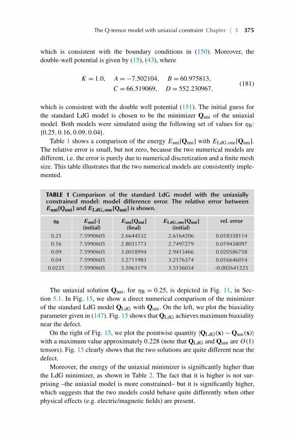
The Q-tensor model with uniaxial constraint Chapter | 5 375
which is consistent with the boundary conditions in (150). Moreover, thedouble-well potential is given by (15), (43), where
K = 1.0, A = −7.502104, B = 60.975813,
C = 66.519069, D = 552.230967,(181)
which is consistent with the double well potential (151). The initial guess forthe standard LdG model is chosen to be the minimizer Quni of the uniaxialmodel. Both models were simulated using the following set of values for ηB:{0.25,0.16,0.09,0.04}.
Table 1 shows a comparison of the energy Euni[Quni] with ELdG,one[Quni].The relative error is small, but not zero, because the two numerical models aredifferent, i.e. the error is purely due to numerical discretization and a finite meshsize. This table illustrates that the two numerical models are consistently imple-mented.
TABLE 1 Comparison of the standard LdG model with the uniaxiallyconstrained model: model difference error. The relative error betweenEuni[Quni] and ELdG,one[Quni] is shown.
ηB Euni[·](initial)
Euni[Quni](final)
ELdG,one[Quni](initial)
rel. error
0.25 7.5990605 2.6644532 2.6164206 0.0183581140.16 7.5990605 2.8031773 2.7497279 0.0194380970.09 7.5990605 3.0018994 2.9413466 0.0205867580.04 7.5990605 3.2711983 3.2176374 0.016646014
0.0225 7.5990605 3.5063179 3.5156034 -0.002641225
The uniaxial solution Quni, for ηB = 0.25, is depicted in Fig. 11, in Sec-tion 5.1. In Fig. 15, we show a direct numerical comparison of the minimizerof the standard LdG model QLdG with Quni. On the left, we plot the biaxialityparameter given in (147). Fig. 15 shows that QLdG achieves maximum biaxialitynear the defect.
On the right of Fig. 15, we plot the pointwise quantity |QLdG(x) − Quni(x)|with a maximum value approximately 0.228 (note that QLdG and Quni are O(1)
tensors). Fig. 15 clearly shows that the two solutions are quite different near thedefect.
Moreover, the energy of the uniaxial minimizer is significantly higher thanthe LdG minimizer, as shown in Table 2. The fact that it is higher is not sur-prising –the uniaxial model is more constrained– but it is significantly higher,which suggests that the two models could behave quite differently when otherphysical effects (e.g. electric/magnetic fields) are present.

376 Handbook of Numerical Analysis
FIGURE 15 Comparison of the standard LdG model with uniaxially constrained version, using theSaturn-ring defect as example (Gu and Abbott, 2000) (Section 7). Left: the “standard” one-constantLdG model exhibits maximum “biaxiality” near the defect. Right: the pointwise L2 error betweenthe minimizer from the standard model and the minimizer with uniaxial constraint.
TABLE 2 Comparison of the standard LdG model with the uniaxially con-strained model: final energy error. The relative error between Euni[Quni]and ELdG,one[QLdG] is shown.
ηB Euni[Quni] (final) ELdG,one[QLdG] (final) rel. error0.25 2.6644532 2.1808923 0.221726140.16 2.8031773 2.2931235 0.222427540.09 3.0018994 2.4689709 0.215850460.04 3.2711983 2.7850147 0.17457129
0.0225 3.5063179 3.0643099 0.14424392
8 Conclusion
We discussed the modeling of nematic LCs and their numerical simulation.We compared three models (namely, Oseen-Frank, Ericksen and Landau-de Gennes) for the equilibrium state of LCs. Because most thermotropic LCsdo not exhibit any biaxiality, we focus on uniaxial LCs and compare Erick-sen’s model with a uniaxially-constrained Landau-de Gennes model. For these,we present robust finite element schemes, which �-converge to the continuousproblem as the mesh size tends to zero. For the solution of the resulting non-linear equations, we design gradient flow-type algorithms that are proven to beenergy-decreasing.
We presented a variety of numerical experiments, illustrating the discretiza-tions’ ability to capture non-trivial orientable and (for the Landau-de Gennesmodel) non-orientable defects. Moreover, we incorporated additional energyterms to model colloidal effects and the effect of external fields, such as electricfields. Finally, we gave a detailed numerical study of the effect of imposing the

The Q-tensor model with uniaxial constraint Chapter | 5 377
uniaxial constraint (exactly) in the classic Landau-de Gennes model, which is amajor highlight of this work.
ReferencesAcharya, B.R., Primak, A., Kumar, S., 2004. Biaxial nematic phase in bent-core thermotropic meso-
gens. Physical Review Letters 92, 145506.Adler, J.H., Atherton, T.J., Benson, T.R., Emerson, D.B., MacLachlan, S.P., 2015a. Energy mini-
mization for liquid crystal equilibrium with electric and flexoelectric effects. SIAM Journal onScientific Computing 37 (5), S157–S176.
Adler, J.H., Atherton, T.J., Emerson, D.B., MacLachlan, S.P., 2015b. An energy-minimization finite-element approach for the Frank–Oseen model of nematic liquid crystals. SIAM Journal onNumerical Analysis 53 (5), 2226–2254.
Adler, J.H., Emerson, D.B., MacLachlan, S.P., Manteuffel, T.A., 2016. Constrained optimization forliquid crystal equilibria. SIAM Journal on Scientific Computing 38 (1), B50–B76.
Alama, S., Bronsard, L., Lamy, X., 2016. Analytical description of the Saturn-ring defect in nematiccolloids. Physical Review E 93, 012705.
Alouges, F., 1997. A new algorithm for computing liquid crystal stable configurations: the harmonicmapping case. SIAM Journal on Numerical Analysis 34 (5), 1708–1726.
Ambrosio, L., 1990a. Existence of minimal energy configurations of nematic liquid crystals withvariable degree of orientation. Manuscripta Mathematica 68 (1), 215–228.
Ambrosio, L., 1990b. Regularity of solutions of a degenerate elliptic variational problem.Manuscripta Mathematica 68 (1), 309–326.
Araki, T., Tanaka, H., 2006. Colloidal aggregation in a nematic liquid crystal: topological arrest ofparticles by a single-stroke disclination line. Physical Review Letters 97, 127801.
Bajc, I., Hecht, F., Žumer, S., 2016. A mesh adaptivity scheme on the Landau-de Gennes func-tional minimization case in 3d, and its driving efficiency. Journal of Computational Physics 321,981–996.
Ball, J.M., 2017. Mathematics and liquid crystals. Molecular Crystals and Liquid Crystals 647 (1),1–27.
Ball, J.M., Feireisl, E., Otto, F., 2015. Mathematical Thermodynamics of Complex Fluids. LectureNotes in Mathematics Book Series, vol. 2200. Springer.
Ball, J.M., Majumdar, A., 2010. Nematic liquid crystals: from Maier-Saupe to a continuum theory.Molecular Crystals and Liquid Crystals 525 (1), 1–11.
Ball, J.M., Zarnescu, A., 2007. Orientable and non-orientable director fields for liquid crystals.Proceedings in Applied Mathematics and Mechanics (PAMM) 7 (1), 1050701–1050704.
Ball, J.M., Zarnescu, A., 2011. Orientability and energy minimization in liquid crystal models.Archive for Rational Mechanics and Analysis 202 (2), 493–535.
Barbero, G., Durand, G., 1986. On the validity of the Rapini-Papoular surface anchoring energyform in nematic liquid crystals. Journal de Physique France 47 (12), 2129–2134.
Barrett, J.W., Feng, X., Prohl, A., 2006. Convergence of a fully discrete finite element methodfor a degenerate parabolic system modelling nematic liquid crystals with variable degree oforientation. ESAIM: Mathematical Modelling and Numerical Analysis 40, 175–199.
Bartels, S., 2006. Stability and convergence of finite-element approximation schemes for harmonicmaps. SIAM Journal on Numerical Analysis 43 (1), 220–238.
Bartels, S., 2015. Numerical Methods for Nonlinear Partial Differential Equations, 1st edition.Springer Series in Computational Mathematics. Springer.
Bartels, S., Raisch, A., 2014. Simulation of q-tensor fields with constant orientational order param-eter in the theory of uniaxial nematic liquid crystals. In: Griebel, M. (Ed.), Singular Phenomenaand Scaling in Mathematical Models. Springer International Publishing, pp. 383–412.
Bedford, S., 2016. Function spaces for liquid crystals. Archive for Rational Mechanics and Analy-sis 219 (2), 937–984.

378 Handbook of Numerical Analysis
Biscari, P., Cesana, P., 2007. Ordering effects in electric splay Freedericksz transitions. ContinuumMechanics and Thermodynamics 19 (5), 285–298.
Biscarini, F., Chiccoli, C., Pasini, P., Semeria, F., Zannoni, C., 1995. Phase diagram and orientationalorder in a biaxial lattice model: a Monte Carlo study. Physical Review Letters 75, 1803–1806.
Borthagaray, J.-P., Nochetto, R.H., Walker, S.W., 2020. A structure-preserving FEM for the uniax-ially constrained Q-tensor model of nematic liquid crystals. Numerische Mathematik 145 (4),837–881.
Braides, A., 2002. Gamma-Convergence for Beginners. Oxford Lecture Series in Mathematics andIts Applications, vol. 22. Oxford Scholarship.
Braides, A., 2014. Local Minimization, Variational Evolution and �-Convergence. Lecture Notes inMathematics, vol. 2094. Springer.
Brandts, J.H., Korotov, S., Krížek, M., 2008. The discrete maximum principle for linear simplicialfinite element approximations of a reaction-diffusion problem. Linear Algebra and Its Applica-tions 429 (10), 2344–2357. Special Issue in honor of Richard S. Varga.
Brezis, H., 2003. The interplay between analysis and topology in some nonlinear pde problems.Bulletin of the American Mathematical Society 40, 179–201.
Brezis, H., Coron, J.-M., Lieb, E.H., 1986. Harmonic maps with defects. Communications in Math-ematical Physics 107 (4), 649–705.
Brinkman, W.F., Cladis, P.E., 1982. Defects in liquid crystals. Physics Today 35, 48–56.Burger, M., 2002. A framework for the construction of level set methods for shape optimization and
reconstruction. Interfaces and Free Boundaries 5, 301–329.Calderer, M., Golovaty, D., Lin, F., Liu, C., 2002. Time evolution of nematic liquid crystals with
variable degree of orientation. SIAM Journal on Mathematical Analysis 33 (5), 1033–1047.Changizrezaei, S., Denniston, C., 2017. Heterogeneous colloidal particles immersed in a liquid crys-
tal. Physical Review E 95, 052703.Ciarlet, P., Raviart, P.-A., 1973. Maximum principle and uniform convergence for the finite element
method. Computer Methods in Applied Mechanics and Engineering 2 (1), 17–31.Cohen, R., Lin, S.-Y., Luskin, M., 1989. Relaxation and gradient methods for molecular orientation
in liquid crystals. Computer Physics Communications 53 (1–3), 455–465.Conradi, M., Ravnik, M., Bele, M., Zorko, M., Žumer, S., Muševic, I., 2009. Janus nematic colloids.
Soft Matter 5, 3905–3912.Cruz, P.A., Tomé, M.F., Stewart, I.W., McKee, S., 2013. Numerical solution of the Ericksen-Leslie
dynamic equations for two-dimensional nematic liquid crystal flows. Journal of ComputationalPhysics 247, 109–136.
Copar, S., Ravnik, M., Žumer, S., 2014. Janus nematic colloids with designable valence. Materials 7(6), 4272.
Copar, S., Tkalec, U., Muševic, I., Žumer, S., 2015. Knot theory realizations in nematic colloids.Proceedings of the National Academy of Sciences 112 (6), 1675–1680.
Davis, T., Gartland, E., 1998. Finite element analysis of the Landau-de Gennes minimization prob-lem for liquid crystals. SIAM Journal on Numerical Analysis 35 (1), 336–362.
de Gennes, P.G., Prost, J., 1995. The Physics of Liquid Crystals, 2nd edition. International Series ofMonographs on Physics, vol. 83. Oxford Science Publication, Oxford, UK.
De Giorgi, E., 2006. In: Maso, G.D., Forti, M., Miranda, M., Spagnolo, S.A., Ambrosio, L. (Eds.),Selected Papers. In: Springer Collected Works in Mathematics.
de Jeu, W.H. (Ed.), 2012. Liquid Crystal Elastomers: Materials and Applications. Advances in Poly-mer Science. Springer.
Dierking, I., Marshall, O., Wright, J., Bulleid, N., 2005. Annihilation dynamics of umbilical defectsin nematic liquid crystals under applied electric fields. Physical Review E 71, 061709.
Dogan, G., Morin, P., Nochetto, R.H., Verani, M., 2007. Discrete gradient flows for shape opti-mization and applications. Computer Methods in Applied Mechanics and Engineering 196,3898–3914.
Doostmohammadi, A., Ignés-Mullol, J., Yeomans, J.M., Sagués, F., 2018. Active nematics. NatureCommunications 9, 3246.

The Q-tensor model with uniaxial constraint Chapter | 5 379
Ericksen, J., 1991. Liquid crystals with variable degree of orientation. Archive for Rational Mechan-ics and Analysis 113 (2), 97–120.
Evans, L.C., 1998. Partial Differential Equations. American Mathematical Society, Providence,Rhode Island.
Feynman, R.P., Leighton, R.B., Sands, M., 1964. The Feynman Lectures on Physics. Addison-Wesley Publishing Company.
Fournier, J.-B., Galatola, P., 2005. Modeling planar degenerate wetting and anchoring in nematicliquid crystals. Europhysics Letters (EPL) 72 (3), 403–409.
Freiser, M., 1970. Ordered states of a nematic liquid. Physical Review Letters 24 (19), 1041.Fukuda, J.-i., Stark, H., Yoneya, M., Yokoyama, H., 2004. Dynamics of a nematic liquid crystal
around a spherical particle. Journal of Physics: Condensed Matter 16 (19), S1957–S1968.Gartland Jr, E.C., Palffy-Muhoray, P., Varga, R.S., 1991. Numerical minimization of the Landau-de
Gennes free energy: defects in cylindrical capillaries. Molecular Crystals and Liquid Crys-tals 199 (1), 429–452.
Gartland, J.E.C., Ramage, A., 2015. A renormalized Newton method for liquid crystal director mod-eling. SIAM Journal on Numerical Analysis 53 (1), 251–278.
Giomi, L., 2015. Geometry and topology of turbulence in active nematics. Physical Review X 5,031003.
González, F.M.G., Gutiérrez-Santacreu, J.V., 2013. A linear mixed finite element scheme for a ne-matic Ericksen-Leslie liquid crystal model. ESAIM: Mathematical Modelling and NumericalAnalysis 47, 1433–1464.
Goodby, J.W., 2012. Introduction to defect textures in liquid crystals. In: Chen, J., Cranton, W.,Fihn, M. (Eds.), Handbook of Visual Display Technology. Springer, pp. 1290–1314.
Gramsbergen, E.F., Longa, L., de Jeu, W.H., 1986. Landau theory of the nematic-isotropic phasetransition. Physics Reports 135 (4), 195–257.
Gu, Y., Abbott, N.L., 2000. Observation of Saturn-ring defects around solid microspheres in nematicliquid crystals. Physical Review Letters 85, 4719–4722.
Holzapfel, G.A., 2000. Nonlinear Solid Mechanics: A Continuum Approach for Engineering. JohnWiley & Sons, Inc..
Hoogboom, J., Elemans, J.A., Rowan, A.E., Rasing, T.H., Nolte, R.J., 2007. The developmentof self-assembled liquid crystal display alignment layers. Philosophical Transactions of theRoyal Society of London A: Mathematical, Physical and Engineering Sciences 365 (1855),1553–1576.
Hu, Q., Tai, X.-C., Winther, R., 2009. A saddle point approach to the computation of harmonicmaps. SIAM Journal on Numerical Analysis 47 (2), 1500–1523.
Humar, M., Muševic, I., 2010. 3d microlasers from self-assembled cholesteric liquid-crystal micro-droplets. Optics Express 18 (26), 26995–27003.
Hyon, Y., Kwak, D.Y., Liu, C., 2010. Energetic variational approach in complex fluids: maxi-mum dissipation principle. Discrete and Continuous Dynamical Systems - Series A 26 (4),1291–1304.
Jost, J., 2017. Riemannian Geometry and Geometric Analysis, 7th edition. Springer.Kinderlehrer, D., Walkington, N., Ou, B., 1993. The Elementary Defects of the Oseen-Frank Energy
for a Liquid Crystal. Research report. Carnegie Mellon University, Department of Mathematics,Center for Nonlinear Analysis.
Korotov, S., Krížek, M., Neittaanmäkia, P., 2001. Weakened acute type condition for tetrahedraltriangulations and the discrete maximum principle. Mathematics of Computation 70 (233),107–119.
Lagerwall, J.P., Scalia, G., 2012. A new era for liquid crystal research: applications of liquid crystalsin soft matter nano-, bio- and microtechnology. Current Applied Physics 12 (6), 1387–1412.
Lamy, X., 2013. A new light on the breaking of uniaxial symmetry in nematics. ArXiv e-prints.Lee, G.-D., Anderson, J., Bos, P.J., 2002. Fast q-tensor method for modeling liquid crystal director
configurations with defects. Applied Physics Letters 81 (21), 3951–3953.

380 Handbook of Numerical Analysis
Lehmann, O., 1889. Über fliessende krystalle (On flowing crystals). Zeitschrift für PhysikalischeChemie 4U, 462–472.
Lin, F.H., 1991. On nematic liquid crystals with variable degree of orientation. Communications onPure and Applied Mathematics 44 (4), 453–468.
Lin, F.-H., Liu, C., 1995. Nonparabolic dissipative systems modeling the flow of liquid crystals.Communications on Pure and Applied Mathematics 48 (5), 501–537.
Lin, F.-H., Liu, C., 2001. Static and dynamic theories of liquid crystals. Journal of Partial DifferentialEquations 14 (4), 289–330.
Lin, S.-Y., Luskin, M., 1989. Relaxation methods for liquid crystal problems. SIAM Journal onNumerical Analysis 26 (6), 1310–1324.
Liu, C., Walkington, N., 2000. Approximation of liquid crystal flows. SIAM Journal on NumericalAnalysis 37 (3), 725–741.
Luckhurst, G., Veracini, C. (Eds.), 1994. The Molecular Dynamics of Liquid Crystals. Nato ScienceSeries C, vol. 431. Springer.
Madsen, L.A., Dingemans, T.J., Nakata, M., Samulski, E.T., 2004. Thermotropic biaxial nematicliquid crystals. Physical Review Letters 92, 145505.
Majumdar, A., 2010. Equilibrium order parameters of nematic liquid crystals in the Landau-deGennes theory. European Journal of Applied Mathematics 21 (2), 181–203.
Majumdar, A., Zarnescu, A., 2010. Landau-de Gennes theory of nematic liquid crystals: the Oseen-Frank limit and beyond. Archive for Rational Mechanics and Analysis 196 (1), 227–280.
Marchetti, M.C., Joanny, J.F., Ramaswamy, S., Liverpool, T.B., Prost, J., Rao, M., Simha, R.A.,2013. Hydrodynamics of soft active matter. Reviews of Modern Physics 85, 1143–1189.
Miles, C.J., Evans, A.A., Shelley, M.J., Spagnolie, S.E., 2019. Active matter invasion of a viscousfluid: unstable sheets and a no-flow theorem. Physical Review Letters 122, 098002.
Moreno-Razo, J.A., Sambriski, E.J., Abbott, N.L., Hernández-Ortiz, J.P., de Pablo, J.J., 2012.Liquid-crystal-mediated self-assembly at nanodroplet interfaces. Nature 485 (7396), 86–89.
Mottram, N.J., Newton, C.J.P., 2014. Introduction to Q-tensor theory. ArXiv e-prints.Mottram, N.J., Pinto, J.T., McKay, G., 2013. Decoupling of the Ericksen-Leslie equations. Liquid
Crystals 40 (6), 787–798.Nguyen, L., Zarnescu, A., 2013. Refined approximation for minimizers of a Landau-de Gennes
energy functional. Calculus of Variations and Partial Differential Equations 47 (1–2), 383–432.Nochetto, R.H., Walker, S.W., Zhang, W., 2015. Numerics for liquid crystals with variable degree
of orientation. In: Symposium NN - Mathematical and Computational Aspects of MaterialsScience. In: MRS Proceedings, vol. 1753.
Nochetto, R.H., Walker, S.W., Zhang, W., 2017. A finite element method for nematic liquid crystalswith variable degree of orientation. SIAM Journal on Numerical Analysis 55 (3), 1357–1386.
Nochetto, R.H., Walker, S.W., Zhang, W., 2018. The Ericksen model of liquid crystals with colloidaland electric effects. Journal of Computational Physics 352, 568–601.
Ohzono, T., Katoh, K., Wang, C., Fukazawa, A., Yamaguchi, S., Fukuda, J.-i., 2017. Uncoveringdifferent states of topological defects in schlieren textures of a nematic liquid crystal. ScientificReports 7 (1), 16814.
Onsager, L., 1931a. Reciprocal relations in irreversible processes. I. Physical Review 37, 405–426.Onsager, L., 1931b. Reciprocal relations in irreversible processes. II. Physical Review 38,
2265–2279.Palffy-muhoray, P., Gartland, E.C., Kelly, J.R., 1994. A new configurational transition in inhomo-
geneous nematics. Liquid Crystals 16 (4), 713–718.Prasad, V., Kang, S.-W., Suresh, K., Joshi, L., Wang, Q., Kumar, S., 2005. Thermotropic uniaxial and
biaxial nematic and smectic phases in bent-core mesogens. Journal of the American ChemicalSociety 127 (49), 17224–17227.
Qian, T., Wang, X.-P., Sheng, P., 2006. A variational approach to moving contact line hydrodynam-ics. Journal of Fluid Mechanics 564, 333–360.
Ramaswamy, S., 2010. The mechanics and statistics of active matter. Annual Review of CondensedMatter Physics 1 (1), 323–345.

The Q-tensor model with uniaxial constraint Chapter | 5 381
Ramaswamy, S., 2017. Active matter. Journal of Statistical Mechanics: Theory and Experiment 2017(5), 054002.
Ravnik, M., Žumer, S., 2009. Landau-de Gennes modelling of nematic liquid crystal colloids. LiquidCrystals 36 (10–11), 1201–1214.
Reinitzer, F., 1888. Beiträge zur kenntniss des cholesterins. Monatshefte für Chemie und VerwandteTeile Anderer Wissenschaften 9 (1), 421–441.
Reinitzer, F., 1989. Contributions to the knowledge of cholesterol. Liquid Crystals 5 (1), 7–18.Roques-Carmes, T., Hayes, R.A., Feenstra, B.J., Schlangen, L.J.M., 2004. Liquid behavior inside a
reflective display pixel based on electrowetting. Journal of Applied Physics 95 (8), 4389–4396.Schoen, R., Uhlenbeck, K., 1982. A regularity theory for harmonic maps. Journal of Differential
Geometry 17 (2), 307–335.Schoen, R., Yau, S.-T., 1994. Lectures on Harmonic Maps. International Press of Boston.Schwartz, M., Lenzini, G., Geng, Y., Rønne, P.B., Ryan, P.Y.A., Lagerwall, J.P.F., 2018. Cholesteric
liquid crystal shells as enabling material for information-rich design and architecture. AdvancedMaterials 30 (30), 1707382.
Shen, J., Yang, X., 2010a. Numerical approximations of Allen-Cahn and Cahn-Hilliard equations.Discrete and Continuous Dynamical Systems 28 (4), 1669–1691.
Shen, J., Yang, X., 2010b. A phase-field model and its numerical approximation for two-phaseincompressible flows with different densities and viscosities. SIAM Journal of Scientific Com-puting 32 (3), 1159–1179.
Sluckin, T.J., Dunmur, D.A., Stegemeyer, H. (Eds.), 2004. Crystals That Flow: Classic Papers Fromthe History of Liquid Crystals, 1st edition. Liquid Crystals Book Series. CRC.
Sluckin, T.J., Poniewierski, A., 1985. Novel surface phase transition in nematic liquid crystals:wetting and the Kosterlitz-Thouless transition. Physical Review Letters 55, 2907–2910.
Sonnet, A., Kilian, A., Hess, S., 1995. Alignment tensor versus director: description of defects innematic liquid crystals. Physical Review E 52, 718–722.
Sonnet, A.M., Virga, E., 2012. Dissipative Ordered Fluids: Theories for Liquid Crystals. Springer.Strang, G., Fix, G., 2008. An Analysis of the Finite Element Method, 2nd edition. Wellesley-
Cambridge.Struwe, M., 2008. Variational Methods: Applications to Nonlinear Partial Differential Equations
and Hamiltonian Systems, 4th edition. Springer.Teixeira-Souza, R.T., Chiccoli, C., Pasini, P., Evangelista, L.R., Zannoni, C., 2015. Nematic liquid
crystals in planar and cylindrical hybrid cells: role of elastic anisotropy on the director defor-mations. Physical Review E 92, 012501.
Temam, R.M., Miranville, A.M., 2005. Mathematical Modeling in Continuum Mechanics, 2nd edi-tion. Cambridge University Press.
Tojo, K., Furukawa, A., Araki, T., Onuki, A., 2009. Defect structures in nematic liquid crystalsaround charged particles. The European Physical Journal E 30 (1), 55–64.
Truesdell, C.A., 1976. A First Course in Rational Continuum Mechanics. Pure and Applied Mathe-matics, a Series of Monographs and Textbooks. Academic Press.
Vanzo, D., Ricci, M., Berardi, R., Zannoni, C., 2012. Shape, chirality and internal order of freelysuspended nematic nanodroplets. Soft Matter 8, 11790–11800.
Vicsek, T., Zafeiris, A., 2012. Collective motion. Physics Reports 517 (3), 71–140. Collective mo-tion.
Virga, E.G., 1994. Variational Theories for Liquid Crystals, vol. 8, 1st edition. Chapman and Hall,London.
Walker, S.W., 2018. On the Correct Thermo-dynamic Potential for Electro-static Dielectric Energy.ArXiv e-prints.
Walkington, N.J., 2011. Numerical approximation of nematic liquid crystal flows governed bythe Ericksen-Leslie equations. ESAIM: Mathematical Modelling and Numerical Analysis 45,523–540.
Wang, X., Kim, Y.-K., Bukusoglu, E., Zhang, B., Miller, D.S., Abbott, N.L., 2016. Experimentalinsights into the nanostructure of the cores of topological defects in liquid crystals. PhysicalReview Letters 116, 147801.

382 Handbook of Numerical Analysis
Whitmer, J.K., Wang, X., Mondiot, F., Miller, D.S., Abbott, N.L., de Pablo, J.J., 2013. Nematic-field-driven positioning of particles in liquid crystal droplets. Physical Review Letters 111,227801.
Wise, S.M., Wang, C., Lowengrub, J.S., 2009. An energy-stable and convergent finite-differencescheme for the phase field crystal equation. SIAM Journal on Numerical Analysis 47 (3),2269–2288.
Xu, J., Li, Y., Wu, S., Bousquet, A., 2019. On the stability and accuracy of partially and fullyimplicit schemes for phase field modeling. Computer Methods in Applied Mechanics and En-gineering 345, 826–853.
Yang, X., Forest, M.G., Li, H., Liu, C., Shen, J., Wang, Q., Chen, F., 2013. Modeling and simulationsof drop pinch-off from liquid crystal filaments and the leaky liquid crystal faucet immersed inviscous fluids. Journal of Computational Physics 236, 1–14.
Yu, L., Saupe, A., 1980. Observation of a biaxial nematic phase in potassium laurate-1-decanol-water mixtures. Physical Review Letters 45 (12), 1000.
Zhao, J., Wang, Q., 2016. Semi-discrete energy-stable schemes for a tensor-based hydrodynamicmodel of nematic liquid crystal flows. Journal of Scientific Computing 68 (3), 1241–1266.
Zhao, J., Yang, X., Shen, J., Wang, Q., 2016. A decoupled energy stable scheme for a hydrody-namic phase-field model of mixtures of nematic liquid crystals and viscous fluids. Journal ofComputational Physics 305, 539–556.