chapter 6 computational models of inferior colliculus...
TRANSCRIPT

BookID 139351_ChapID 6_Proof# 1 - 18/01/2010
Abbreviations
AM Amplitude modulationAN Auditory nerveBD Best delayBMF Best modulation frequencyBF Best frequencyCD Characteristic delayCN Cochlear nucleusCP Characteristic phaseCR Chopping rateDCN Dorsal cochlear nucleusDNLL Dorsal nucleus of the lateral lemniscusEI Contralaterally excited and ipsilaterally inhibitedEI/F EI with facilitationF0 Fundamental frequencyIC Inferior colliculusICC Central nucleus of the inferior colliculusICX External nucleus of the inferior colliculusILD Interaural level differenceIPD Interaural phase differenceITD Interaural time differenceLSO Lateral superior olive
K.A. Davis (*) Departments of Biomedical Engineering and Neurobiology and Anatomy, University of Rochester, Rochester, NY 14642, USA e-mail: [email protected]
Chapter 6Computational Models of Inferior Colliculus Neurons
Kevin A. Davis, Kenneth E. Hancock, and Bertrand Delgutte[AU1]
R. Meddis et al. (eds.), Computational Models of the Auditory System, Springer Handbook of Auditory Research 35, DOI 10.1007/978-1-4419-5934-8_6, © Springer Science+Business Media, LLC 2010
0001135906.INDD 1 1/18/2010 4:04:26 PM
1
2
3
4
5
6
7
8
9
10
11
12
13
14
15
16
17
18
19
20
21
22
23
24
25
26

BookID 139351_ChapID 6_Proof# 1 - 18/01/2010
K.A. Davis et al.
MNTB Medial nucleus of the trapezoid bodyMSO Medial superior oliveMTF Modulation transfer functionPE Precedence effectPIR Postinhibitory reboundSOC Superior olivary complexVNLL Ventral nucleus of the lateral lemniscusVCN Ventral cochlear nucleus
6.1 Introduction
The inferior colliculus (IC), the principal auditory nucleus in the midbrain, occupies a key position in the auditory system. It receives convergent input from most of the auditory nuclei in the brain stem, and in turn, projects to the auditory forebrain (Winer and Schreiner 2005). The IC is therefore a major site for the integration and reorganization of the different types of auditory informa-tion conveyed by largely parallel neural pathways in the brain stem, and its neural response properties are accordingly very diverse and complex (Winer and Schreiner 2005). The function of the IC has been hard to pinpoint. The IC has been called the “nexus of the auditory pathway” (Aitkin 1986), a “shunting yard of acoustical information processing” (Ehret and Romand 1997), and the locus of a “transformation [that] adjusts the pace of sensory input to the pace of behavior” (Casseday and Covey 1996). The vague, if not metaphorical, nature of these descriptions partly reflects the lack of a quantitative understand-ing of IC processing such as that which has emerged from computational stud-ies of the cochlear nucleus (Voigt, Chap. 3) and superior olivary complex (Colburn, Chap. 4).
This chapter reviews computational modeling efforts aimed at understanding how the representations of the acoustic environment conveyed by the ascending inputs are processed and integrated in the IC. Most of these efforts have been directed at the processing of either sound localization cues or amplitude envelope information. To our knowledge, this is the first detailed review of this topic, although previous reviews of the processing of specific stimulus features, for example, binaural processing (Colburn 1996; Palmer and Kuwada 2005) or tempo-ral processing (Langner 1992; Rees and Langner 2005) briefly discussed models for IC neurons. Our focus is primarily on models aimed at explaining biophysical mechanisms leading to emerging physiological response properties of individual IC neurons, although some neural population models for predicting psychophysical performance from patterns of neural activity are also covered. The models are restricted to the mammalian IC, with the exception of one model for the avian homolog of the IC (Rucci and Wray 1999) where the processing may be of general applicability.
0001135906.INDD 2 1/18/2010 4:04:26 PM
27
28
29
30
31
32
33
34
35
36
37
38
39
40
41
42
43
44
45
46
47
48
49
50
51
52
53
54
55
56
57
58
59
60
61
62
63
64
65
66
BookID 139351_ChapID 6_Proof# 1 - 18/01/2010
6 Computational Models of Inferior Colliculus Neurons
6.1.1 Functional Organization and Afferent Projections to the Inferior Colliculus
The IC consists of a central nucleus (ICC), characterized by the presence of disk-shaped cells and fibrodendritic laminae, surrounded by layered structures (“cor-tices”) dorsally, laterally, and caudally (Oliver 2005). The tonotopically organized ICC receives the vast majority of afferent inputs from brain stem auditory nuclei and has been the object of most neurophysiological and modeling studies. The surrounding regions receive multisensory and descending inputs as well as ascending projections from the brain stem and ICC, and neurons in these subdivisions tend to have more complex and labile response properties than those in ICC. The main focus of this chapter is therefore on models for ICC neurons.
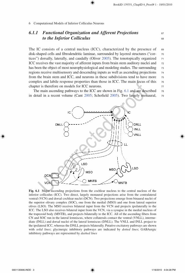
The main ascending pathways to the ICC are shown in Fig. 6.1 and are described in detail in a recent volume (Cant 2005; Schofield 2005). Two largely monaural,
Fig. 6.1 Major ascending projections from the cochlear nucleus to the central nucleus of the inferior colliculus (ICC). Two direct, largely monaural projections arise from the contralateral ventral (VCN) and dorsal cochlear nuclei (DCN). Two projections emerge from binaural nuclei of the superior olivary complex (SOC), one from the medial (MSO) and one from lateral superior olives (LSO). The MSO receives bilateral input from the VCN and projects ipsilaterally to the ICC. The LSO also receives bilateral input from the VCN, via a synapse in the medial nucleus of the trapezoid body (MNTB), and projects bilaterally to the ICC. All of the ascending fibers from CN and SOC run in the lateral lemniscus, where collaterals contact the ventral (VNLL), interme-diate (INLL) and dorsal nuclei of the lateral lemniscus (DNLL). The VNLL and INLL project to the ipsilateral ICC, whereas the DNLL projects bilaterally. Putative excitatory pathways are shown with solid lines; glycinergic inhibitory pathways are indicated by dotted lines; GABAergic inhibitory pathways are represented by dashed lines
0001135906.INDD 3 1/18/2010 4:04:28 PM
67
68
69
70
71
72
73
74
75
76
77
78
79
BookID 139351_ChapID 6_Proof# 1 - 18/01/2010
K.A. Davis et al.
excitatory projections to the ICC emerge from the stellate cells in the contralateral ventral cochlear nucleus (VCN) and the fusiform and giant cells in the contralat-eral dorsal cochlear nucleus (DCN) (Cant 2005). The ICC also receives major projections from the two main binaural nuclei of the superior olivary complex (SOC): an ipsilateral excitatory projection from the medial superior olive (MSO) and bilateral projections from the lateral superior olives (LSO) (Schofield 2005). The crossed LSO projection is excitatory, whereas the uncrossed projection is mostly inhibitory and glycinergic (Schofield 2005). LSO neurons show sensitiv-ity to interaural level differences (ILD) arising through interaction of an excit-atory input from spherical bushy cells in the ipsilateral VCN, and an inhibitory input from globular bushy cells in the contralateral VCN via an intervening syn-apse in the medial nucleus of the trapezoid body (MNTB). In contrast, MSO neurons show sensitivity to interaural time differences (ITD) created by conver-gence of bilateral excitatory inputs from spherical bushy cells in the VCN, with modulation by additional inhibitory inputs.
In addition to ascending projections from the cochlear nuclei (CN) and the SOC, the ICC receives afferent input from three groups of neurons intermingled among the lateral lemniscus fibers ascending to the auditory midbrain: the ventral (VNLL), intermediate (INLL), and dorsal nuclei of the lateral lemniscus (DNLL) (Schofield 2005). The most important of these for our purposes are the DNLL projections, which are bilateral and mostly GABAergic. The DNLL receives most of its inputs from binaural nuclei including MSO, LSO, and the contralateral DNLL, and contains many neurons sensitive to ITD and ILD.
The various brain stem projections to the ICC overlap in some locations, but remain partly segregated in other regions, forming unique synaptic (functional) domains (Oliver and Huerta 1992). The development of physiological criteria for identifying the brain stem cell types from which an ICC neuron receives inputs is an active area of research (Oliver et al. 1997; Ramachandran et al. 1999; Davis 2002; Loftus et al. 2004; Malmierca et al. 2005).
By traditional anatomical criteria, there are only two types of neurons in ICC: disc-shaped and stellate (Oliver and Morest 1984). Disc-shaped cells form the vast majority of ICC neurons, and have planar dendritic fields parallel to the tonotopi-cally-organized afferent fibers from the lateral lemniscus. Stellate cells have omni-directional dendritic fields spanning several fibrodendritic laminae formed by the lemniscal axons and the dendrites of disc-shaped cells. The physiological corre-lates of these two anatomical cell types are unknown. In vitro recordings reveal a more complex organization than the traditional disc-shaped/stellate dichotomy. For example, Sivaramakrishnan and Oliver (2001) have identified six physiologi-cally distinct cell types based on their membrane composition in various types of K+ channels. How the different types of ICC cells defined by intrinsic membrane channels interact with the wide diversity of synaptic domains based on afferent inputs is still an unexplored topic. It is clear, however, that the highly complex organization of the ICC provides a framework for sophisticated processing of acoustic information.
0001135906.INDD 4 1/18/2010 4:04:28 PM
80
81
82
83
84
85
86
87
88
89
90
91
92
93
94
95
96
97
98
99
100
101
102
103
104
105
106
107
108
109
110
111
112
113
114
115
116
117
118
119
120
121
122
123
BookID 139351_ChapID 6_Proof# 1 - 18/01/2010
6 Computational Models of Inferior Colliculus Neurons
6.1.2 Strategies for Modeling IC Neurons
The great complexity in the functional organization and afferent inputs of the ICC necessarily calls for simplification when modeling the response properties of ICC neurons. To distinguish processing occurring in the IC itself from that inherited from the inputs, an ICC neuron model must include a functional description of the inputs to the IC, that is, it must explicitly or implicitly incorporate a model for processing by the auditory periphery and brain stem nuclei. The models discussed in this chapter illustrate different approaches to this general problem.
The most detailed models explicitly generate action potentials at every stage in the auditory pathway from the auditory nerve (AN) to the IC (Hewitt and Meddis 1994; Cai et al. 1998a, b; Shackleton et al. 2000; Kimball et al. 2003; Voutsas et al. 2005; Dicke et al. 2007; Pecka et al. 2007). This approach has the advantage of directly mimicking the biology, and with a modular software architecture, any improve-ment in modeling one neuron module can, in principle, be readily propagated to the entire circuit. However, this type of model can be computationally demanding and is limited by the weakest link in the chain of neuron models.
In many cases, the models for individual neurons in the circuit are single-compartment models with explicit biophysical simulation of selected membrane channels; synaptic inputs are implemented as changes in a membrane conductance (Hewitt and Meddis 1994; Cai et al. 1998a, b; Shackleton et al. 2000; Kimball et al. 2003; Pecka et al. 2007). These models generate an action potential when the mem-brane voltage crosses a threshold (often time-varying). However, some models intro-duce simplifications in the simulations for at least some of the neurons in the circuit. Some models use point process models rather than biophysical simulations to gen-erate spikes efficiently (Dicke et al. 2007), some replace spiking neuron models by models operating on firing probabilities (Nelson and Carney 2004), and some use algebraic steady-state input–output functions to model the transformations in average firing rates through the circuit (Reed and Blum 1999; Rucci and Wray 1999). These simplifications can increase computational efficiency but also preclude a char-acterization of certain response properties, for example, temporal discharge pat-terns when using input–output functions operating on average firing rates, or the influence of firing history (e.g., refractoriness) when using spike probabilities.
Some IC models avoid an explicit modeling of the brain stem circuitry altogether, using signal processing models (such as cross-correlation) to simulate either the immediate inputs to the IC (Rucci and Wray 1999; Borisyuk et al. 2002) or the IC responses themselves (Hancock and Delgutte 2004). Again, this can achieve con-siderable computational efficiency that is particularly important when modeling a large population of IC neurons (Rucci and Wray 1999; Hancock and Delgutte 2004) but can also limit the set of stimuli to which the model is applicable (e.g., the Borisyuk et al. 2002 model only applies to sinusoidal stimuli, and the cross-correlation models work best for static stimuli).
The models also differ in which subsets of inputs to the ICC they include. Models for binaural processing explicitly include modules for the SOC inputs
0001135906.INDD 5 1/18/2010 4:04:28 PM
124
125
126
127
128
129
130
131
132
133
134
135
136
137
138
139
140
141
142
143
144
145
146
147
148
149
150
151
152
153
154
155
156
157
158
159
160
161
162
163
164
165
166

BookID 139351_ChapID 6_Proof# 1 - 18/01/2010
K.A. Davis et al.
(Cai et al. 1998a, b; Shackleton et al. 2000; Pecka et al. 2007), while models for spectral processing (Kimball et al. 2003) focus on inputs from DCN, and models for temporal processing of amplitude modulation (AM) information typically focus on inputs from VCN (Hewitt and Meddis 1994; Nelson and Carney 2004; Voutsas et al. 2005; Dicke et al. 2007). Among the binaural models, those concerned with ITD processing tend to include primarily inputs from MSO and, in some cases, DNLL (Cai et al. 1998a, b; Borisyuk et al. 2002), while models for ILD processing include only inputs from the LSO circuit (Reed and Blum 1999; Pecka et al. 2007). Only one binaural model includes inputs from both MSO and LSO (Shackleton et al. 2000), although even in this case the focus is limited to ITD processing.
6.2 Sound Localization in an Anechoic Environment
Our ability to localize sounds in space is based primarily on three acoustic cues: interaural differences in time and level, and spectral cues (Middlebrooks and Green 1991). The first two cues arise as a result of the spatial separation of the two ears, and are important for left–right (azimuthal) localization. Spectral cues are created by the filtering properties of the head and pinnae, and are critical for accurate local-ization of elevation in the median plane where interaural cues are minimal. Initial processing of these three cues is done largely in separate brain stem nuclei, with ITD encoded in the MSO (Goldberg and Brown 1969; Yin and Chan 1990), ILD in the LSO (Boudreau and Tsuchitani 1968), and spectral cues (in the form of spectral notches) in the DCN (Young and Davis 2001). Neurons sensitive to binaural and/or monaural sound localization cues are common in the ICC (Palmer and Kuwada 2005). In some respects, the response properties of these ICC neurons are similar to those of their brain stem inputs, but there are also important differences on which modeling efforts have been focused.
6.2.1 Lateralization Based on ITD
One difference between neurons in the brain stem and the midbrain is that ICC unit sensitivity to ITD is often incompatible with a simple coincidence detection mecha-nism (Jeffress 1948). Most neurons in the MSO respond maximally when their inputs from the two sides arrive simultaneously, that is, they act as interaural coincidence detectors (Goldberg and Brown 1969). These units are termed “peak type” because their pure-tone ITD functions show a maximum response (peak) at the same ITD (called characteristic delay, CD) regardless of stimulus frequency (Yin and Chan 1990). The CD is defined as the slope of the function relating best interaural phase to stimulus frequency (the phase plot), which for simple coincidence detectors is a straight line with a y-intercept (the characteristic phase, CP) equal to 0 cycle (dashed line, Fig. 6.2a). Other brain stem neurons, most notably in the LSO, are excited by
0001135906.INDD 6 1/18/2010 4:04:28 PM
167
168
169
170
171
172
173
174
175
176
177
178
179
180
181
182
183
184
185
186
187
188
189
190
191
192
193
194
195
196
197
198
199
200
201
202
203

BookID 139351_ChapID 6_Proof# 1 - 18/01/2010
6 Computational Models of Inferior Colliculus Neurons
Fig. 6.2 Schematic representations of transformations in binaural and monaural response proper-ties between the brain stem and the midbrain. (a) Phase plots derived from responses to binaural pure tones for ITD-sensitive unit(s) in the MSO (peak-type; dashed line), the LSO (trough-type; dotted line) and the ICC (intermediate (i) and complex-types (c); solid lines). (b) Rate vs. ILD curves for an excitatory–inhibitory (EI) unit in the LSO (dashed line) and an EI/F unit in the ICC (solid line). (c) Responses of a DCN type IV unit (dashed line) and an ICC type O unit (solid line) to a notched-noise stimulus whose 3.2-kHz wide notch is swept across the receptive field of the unit. The gray bar indicates the range of spontaneous rates for the two units. (d) Population response recovery functions to the second of a pair of binaural clicks for CN units (dashed line) and ICC units (solid line). (e) Interaural phase difference (IPD) functions of an MSO (dashed line) and an ICC neuron (solid lines) derived from responses to simulated sound motion through arcs in the azimuthal plane (sweeps are shown with arrows at the top of the plot). (f) Rate modulation transfer functions for a CN (dashed line) and an ICC unit (solid line)
[AU2]
0001135906.INDD 7 1/18/2010 4:04:29 PM
BookID 139351_ChapID 6_Proof# 1 - 18/01/2010
K.A. Davis et al.
sounds in the ipsilateral ear and inhibited by sounds in the contralateral ear (Boudreau and Tsuchitani 1968). Although the spatial receptive fields of LSO units are domi-nated by ILD cues (Tollin and Yin 2002a, b), many LSO units are also ITD sensitive and are termed “trough type” because they respond minimally when binaural inputs of any frequency are in phase (Caird and Klinke 1983). The phase plots of trough types units are also linear, but with a CP of 0.5 cycle (dotted line, Fig. 6.2a).
In the ICC, many neurons show peak-type and trough-type ITD functions similar to those of MSO and LSO neurons, respectively (Yin and Kuwada 1983). Many other units, however, diverge from the simple coincidence detector model (solid lines, Fig. 6.2a) and show either linear phase plots whose CP is neither 0 nor 0.5 cycles (“intermediate types”) or nonlinear phase plots (“complex type”) (Palmer and Kuwada 2005). Intermediate and complex type neurons are also observed in the SOC, but they appear to be less prevalent than in ICC (Batra et al. 1997a). It has been hypothesized that the additional complexities of ICC binaural responses may be created through convergence of peak and trough type inputs within the ICC (Yin and Kuwada 1983; McAlpine et al. 1998), or may reflect the effects of ITD-sensitive inhibitory inputs (McAlpine et al. 1998).
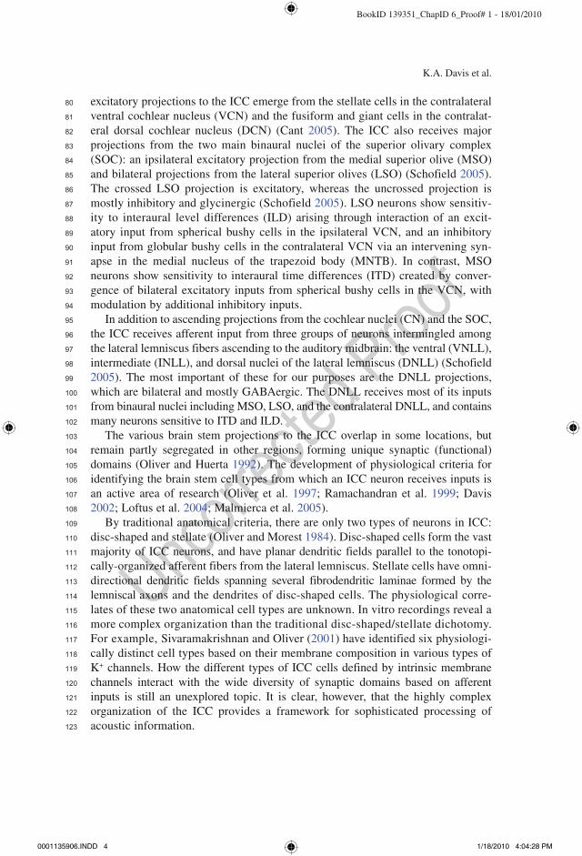
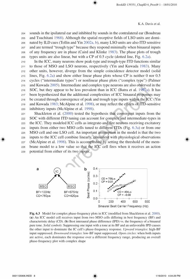
Shackleton et al. (2000) tested the hypothesis that convergent inputs from the SOC with different ITD tuning can account for complex and intermediate-types in the ICC. They modeled ICC cells as integrate-and-fire neurons receiving excitatory inputs from either two MSO cells tuned to different ITDs (Fig. 6.3a) or from one MSO cell and one LSO cell. An important assumption in the model is that the two inputs to the ICC cell combine linearly, consistent with physiological observations (McAlpine et al. 1998). This is accomplished by setting the threshold of the mem-brane model to a low value so that the ICC cell fires when it receives an action potential from either of its two inputs.
Fig. 6.3 Model for complex phase-frequency plots in ICC (modified from Shackleton et al. 2000). (a) An ICC model cell receives input from two MSO cells differing in best frequency (BF) and characteristic delay (CD). (b) Best interaural phase difference (IPD) vs. the frequency of a binaural pure tone. Solid symbols: Suppressing one input with a tone at its BF and an unfavorable IPD causes the other input to dominate the IC cell’s phase-frequency response. Upward triangles: high-BF input suppressed. Downward triangles: low-BF input suppressed. Open circles: when both inputs are active, each dominates the response over a different frequency range, producing an overall phase-frequency plot with complex shape
0001135906.INDD 8 1/18/2010 4:04:29 PM
204
205
206
207
208
209
210
211
212
213
214
215
216
217
218
219
220
221
222
223
224
225
226
227
228
229
BookID 139351_ChapID 6_Proof# 1 - 18/01/2010
6 Computational Models of Inferior Colliculus Neurons
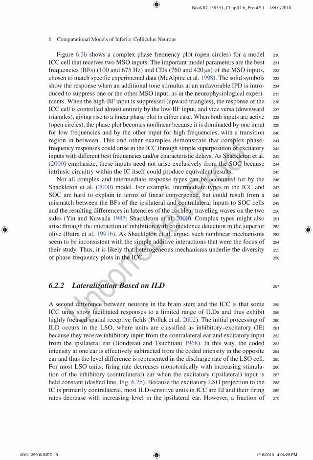
Figure 6.3b shows a complex phase-frequency plot (open circles) for a model ICC cell that receives two MSO inputs. The important model parameters are the best frequencies (BFs) (100 and 675 Hz) and CDs (760 and 420 ms) of the MSO inputs, chosen to match specific experimental data (McAlpine et al. 1998). The solid symbols show the response when an additional tone stimulus at an unfavorable IPD is intro-duced to suppress one or the other MSO input, as in the neurophysiological experi-ments. When the high-BF input is suppressed (upward triangles), the response of the ICC cell is controlled almost entirely by the low-BF input, and vice versa (downward triangles), giving rise to a linear phase plot in either case. When both inputs are active (open circles), the phase plot becomes nonlinear because it is dominated by one input for low frequencies and by the other input for high frequencies, with a transition region in between. This and other examples demonstrate that complex phase-frequency responses could arise in the ICC through simple superposition of excitatory inputs with different best frequencies and/or characteristic delays. As Shackleton et al. (2000) emphasize, these inputs need not arise exclusively from the SOC because intrinsic circuitry within the IC itself could produce equivalent results.
Not all complex and intermediate response types can be accounted for by the Shackleton et al. (2000) model. For example, intermediate types in the ICC and SOC are hard to explain in terms of linear convergence, but could result from a mismatch between the BFs of the ipsilateral and contralateral inputs to SOC cells and the resulting differences in latencies of the cochlear traveling waves on the two sides (Yin and Kuwada 1983; Shackleton et al. 2000). Complex types might also arise through the interaction of inhibition with coincidence detection in the superior olive (Batra et al. 1997b). As Shackleton et al. argue, such nonlinear mechanisms seem to be inconsistent with the simple additive interactions that were the focus of their study. Thus, it is likely that heterogeneous mechanisms underlie the diversity of phase-frequency plots in the ICC.
6.2.2 Lateralization Based on ILD
A second difference between neurons in the brain stem and the ICC is that some ICC units show facilitated responses to a limited range of ILDs and thus exhibit highly focused spatial receptive fields (Pollak et al. 2002). The initial processing of ILD occurs in the LSO, where units are classified as inhibitory–excitatory (IE) because they receive inhibitory input from the contralateral ear and excitatory input from the ipsilateral ear (Boudreau and Tsuchitani 1968). In this way, the coded intensity at one ear is effectively subtracted from the coded intensity in the opposite ear and thus the level difference is represented in the discharge rate of the LSO cell. For most LSO units, firing rate decreases monotonically with increasing stimula-tion of the inhibitory (contralateral) ear when the excitatory (ipsilateral) input is held constant (dashed line, Fig. 6.2b). Because the excitatory LSO projection to the IC is primarily contralateral, most ILD-sensitive units in ICC are EI and their firing rates decrease with increasing level in the ipsilateral ear. However, a fraction of
0001135906.INDD 9 1/18/2010 4:04:29 PM
230
231
232
233
234
235
236
237
238
239
240
241
242
243
244
245
246
247
248
249
250
251
252
253
254
255
256
257
258
259
260
261
262
263
264
265
266
267
268
269
270
BookID 139351_ChapID 6_Proof# 1 - 18/01/2010
K.A. Davis et al.
units (~20%) shows facilitation at intermediate levels of ipsilateral stimulation and inhibition at higher levels (EI/F cells) (solid line, Fig. 6.2b) (Park and Pollak 1993; Davis et al. 1999). These neurons could be the basis for a “place code” of ILD, because they have relatively circumscribed receptive fields. Blocking GABAergic inhibition in the ICC transforms most EI/F cells into conventional EI cells by increasing the spike count elicited by the contralateral sound (Park and Pollak 1993). Hence, the term “facilitation” is somewhat misleading: the essential feature of EI/F cells appears to be GABAergic inhibition evoked by high-level sounds in the contralateral ear. The ipsilateral DNLL has been suggested as the source of this inhibition (Park and Pollak 1993).
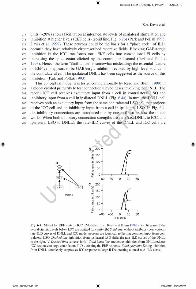
This conceptual model was tested computationally by Reed and Blum (1999) in a model created primarily to test connectional hypotheses involving the DNLL. The model ICC cell receives excitatory input from a cell in contralateral LSO and inhibitory input from a cell in ipsilateral DNLL (Fig. 6.4a). In turn, the DNLL cell receives both an excitatory input from the same contralateral LSO cell that projects to the ICC cell and an inhibitory input from a cell in ipsilateral LSO. In Fig. 6.4, the inhibitory connections are introduced one by one to illustrate how the model works. When both inhibitory connection strengths are zero (i.e., DNLL to ICC, and ipsilateral LSO to DNLL), the rate–ILD curves of the DNLL and ICC cells are
Fig. 6.4 Model for EI/F units in ICC. (Modified from Reed and Blum 1999.) (a) Diagram of the neural circuit. Levels below LSO are omitted for clarity. (b) Solid line: without inhibitory connections, rate–ILD curves of DNLL and ICC model neurons are identical, reflecting common input from con-tralateral LSO. Dashed line: inhibition from ipsilateral LSO shifts the rate–ILD curves of the DNLL to the right. (c) Dashed line: same as in (b). Solid black line: moderate inhibition from DNLL reduces ICC response to large contralateral ILDs, creating the EI/F response. Solid gray line: Strong inhibition from DNLL completely suppresses ICC response to large ILDs, creating a tuned rate–ILD curve
0001135906.INDD 10 1/18/2010 4:04:30 PM
271
272
273
274
275
276
277
278
279
280
281
282
283
284
285
286
287
288
289
BookID 139351_ChapID 6_Proof# 1 - 18/01/2010
6 Computational Models of Inferior Colliculus Neurons
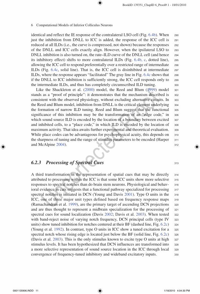
identical and reflect the IE response of the contralateral LSO cell (Fig. 6.4b). When just the inhibition from DNLL to ICC is added, the response of the ICC cell is reduced at all ILDs (i.e., the curve is compressed, not shown) because the responses of the DNLL and ICC cells exactly align. However, when the ipsilateral LSO to DNLL inhibition is also turned on, the rate–ILD curve of the DNLL cell (and hence its inhibitory effect) shifts to more contralateral ILDs (Fig. 6.4b, c, dotted line), allowing the ICC cell to respond preferentially over a restricted range of intermediate ILDs (Fig. 6.4c, solid line). That is, the ICC cell is disinhibited at intermediate ILDs, where the response appears “facilitated” The gray line in Fig. 6.4c shows that if the DNLL to ICC inhibition is sufficiently strong, the ICC cell responds only to the intermediate ILDs, and thus has completely circumscribed ILD tuning.
Like the Shackleton et al. (2000) model, the Reed and Blum (1999) model stands as a “proof of principle”: it demonstrates that the mechanism described is consistent with the observed physiology, without excluding alternative circuits. In the Reed and Blum model, inhibition from DNLL is the critical element underlying the formation of narrow ILD tuning. Reed and Blum suggest that the functional significance of this inhibition may be the transformation of an “edge code,” in which sound source ILD is encoded by the location of a boundary between excited and inhibited cells, to a “place code,” in which ILD is encoded by the location of maximum activity. That idea awaits further experimental and theoretical evaluation. While place codes can be advantageous for psychophysical acuity, this depends on the sharpness of tuning and the range of stimulus parameters to be encoded (Harper and McAlpine 2004).
6.2.3 Processing of Spectral Cues
A third transformation in the representation of spatial cues that may be directly attributed to processing within the ICC is that some ICC units show more selective responses to spectral notches than do brain stem neurons. Physiological and behav-ioral evidence in cats suggests that a functional pathway specialized for processing spectral notches is initiated in DCN (Young and Davis 2001). Type O units in the ICC, one of three major unit types defined based on frequency response maps (Ramachandran et al. 1999), are the primary target of ascending DCN projections and are thus thought to represent a midbrain specialization for the processing of spectral cues for sound localization (Davis 2002; Davis et al. 2003). When tested with band-reject noise of varying notch frequency, DCN principal cells (type IV units) show tuned inhibition for notches centered at their BF (dashed line, Fig. 6.2c) (Young et al. 1992). In contrast, type O units in ICC show a tuned excitation for a spectral notch whose rising edge is located just below the BF (solid line, Fig. 6.2c) (Davis et al. 2003). This is the only stimulus known to excite type O units at high stimulus levels. It has been hypothesized that DCN influences are transformed into a more selective representation of sound source location in the ICC through local convergence of frequency-tuned inhibitory and wideband excitatory inputs.
0001135906.INDD 11 1/18/2010 4:04:30 PM
290
291
292
293
294
295
296
297
298
299
300
301
302
303
304
305
306
307
308
309
310
311
312
313
314
315
316
317
318
319
320
321
322
323
324
325
326
327
328
329
330
BookID 139351_ChapID 6_Proof# 1 - 18/01/2010
K.A. Davis et al.
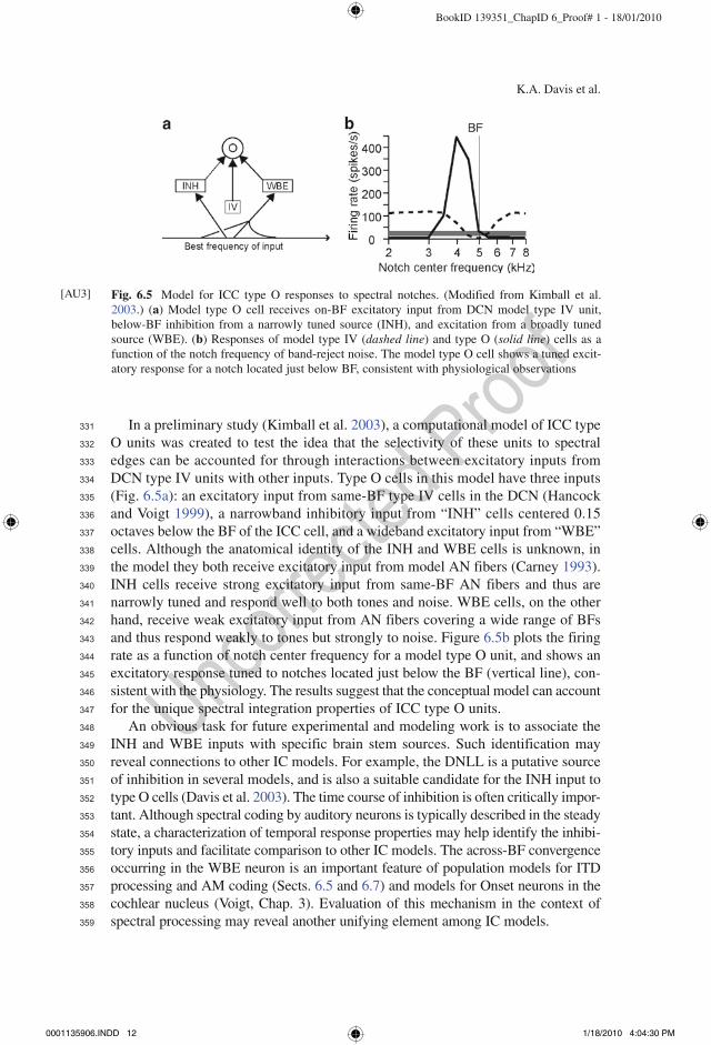
In a preliminary study (Kimball et al. 2003), a computational model of ICC type O units was created to test the idea that the selectivity of these units to spectral edges can be accounted for through interactions between excitatory inputs from DCN type IV units with other inputs. Type O cells in this model have three inputs (Fig. 6.5a): an excitatory input from same-BF type IV cells in the DCN (Hancock and Voigt 1999), a narrowband inhibitory input from “INH” cells centered 0.15 octaves below the BF of the ICC cell, and a wideband excitatory input from “WBE” cells. Although the anatomical identity of the INH and WBE cells is unknown, in the model they both receive excitatory input from model AN fibers (Carney 1993). INH cells receive strong excitatory input from same-BF AN fibers and thus are narrowly tuned and respond well to both tones and noise. WBE cells, on the other hand, receive weak excitatory input from AN fibers covering a wide range of BFs and thus respond weakly to tones but strongly to noise. Figure 6.5b plots the firing rate as a function of notch center frequency for a model type O unit, and shows an excitatory response tuned to notches located just below the BF (vertical line), con-sistent with the physiology. The results suggest that the conceptual model can account for the unique spectral integration properties of ICC type O units.
An obvious task for future experimental and modeling work is to associate the INH and WBE inputs with specific brain stem sources. Such identification may reveal connections to other IC models. For example, the DNLL is a putative source of inhibition in several models, and is also a suitable candidate for the INH input to type O cells (Davis et al. 2003). The time course of inhibition is often critically impor-tant. Although spectral coding by auditory neurons is typically described in the steady state, a characterization of temporal response properties may help identify the inhibi-tory inputs and facilitate comparison to other IC models. The across-BF convergence occurring in the WBE neuron is an important feature of population models for ITD processing and AM coding (Sects. 6.5 and 6.7) and models for Onset neurons in the cochlear nucleus (Voigt, Chap. 3). Evaluation of this mechanism in the context of spectral processing may reveal another unifying element among IC models.
Fig. 6.5 Model for ICC type O responses to spectral notches. (Modified from Kimball et al. 2003.) (a) Model type O cell receives on-BF excitatory input from DCN model type IV unit, below-BF inhibition from a narrowly tuned source (INH), and excitation from a broadly tuned source (WBE). (b) Responses of model type IV (dashed line) and type O (solid line) cells as a function of the notch frequency of band-reject noise. The model type O cell shows a tuned excit-atory response for a notch located just below BF, consistent with physiological observations
[AU3]
0001135906.INDD 12 1/18/2010 4:04:30 PM
331
332
333
334
335
336
337
338
339
340
341
342
343
344
345
346
347
348
349
350
351
352
353
354
355
356
357
358
359

BookID 139351_ChapID 6_Proof# 1 - 18/01/2010
6 Computational Models of Inferior Colliculus Neurons
6.3 Sound Localization in Reverberant Environments: The Precedence Effect
The precedence effect (PE, a.k.a. “law of the first wavefront”) refers to a group of perceptual phenomena relevant to sound localization in reverberant environments (for review, see Litovsky et al. 1999). The PE is experienced when two (or more) sounds originating from different spatial locations reach the ears closely spaced in time. Typically, the leading sound represents the direct wavefront and the lagging sound a single acoustic reflection. If the delay between the two sounds is less than approximately 1 ms, the listener hears a single auditory event located between the two sources, but biased toward the leading source. This phenomenon is called sum-ming localization. For longer delays, the listener still hears only one auditory event but localizes the event near the location of the leading source. This phenomenon is called localization dominance. Finally, if the interstimulus delay exceeds an “echo threshold,” then the two sounds are perceived as separate entities each with its own spatial location. The echo threshold depends on the characteristics of the sound source, ranging from 5 to 10 ms for transient sounds to 30 to 50 ms for continuous speech or music (for review, see Litovsky et al. 1999). It is important to note that, while the spatial location of the lagging sound is suppressed during the period of localization dominance, its presence nonetheless affects other aspects of the percept including its timbre, loudness, and spatial extent.
Neural correlates of the PE have been described at virtually all levels of the audi-tory system, including the auditory nerve, cochlear nucleus, SOC, ICC and auditory cortex (reviewed by Litovsky et al. 1999; Palmer and Kuwada 2005). At each level, when a pair of successive sounds (e.g., clicks) is presented to the ears with a short delay, the response to the lagging stimulus is (almost always) suppressed for short delays and recovers for long delays. The rate of recovery depends on the stage of the auditory system under study. At the level of the AN and CN (dashed line, Fig. 6.2d), neurons typically respond to lag stimuli for delays as short as 1–2 ms, whereas in the ICC (solid line, Fig. 6.2d) and auditory cortex, recovery takes 10–100 ms, although there is considerable variability across neurons. The recovery time in ICC depends on anesthetic state, and is about half as long in awake animals compared to anesthetized animals (Tollin and Yin 2004).
Neural echo suppression observed with pairs of transient stimuli is often inter-preted as a correlate of localization dominance in the PE (Litovsky et al. 1999). Consistent with this interpretation, echo suppression in the ICC is directional and depends on binaural cues (Litovsky and Yin 1998). For example, in some neurons, a leading stimulus at the neuron’s best ITD evokes stronger suppression than a stimulus at the worst ITD; in other neurons, the converse is true. On the other hand, neural echo suppression is observed with similar properties in binaural and monaural neurons, so that some forms of suppression may represent a more general correlate of context dependent perceptual phenomena (such as forward masking) rather than being specifically linked to the PE. The long duration of echo suppression in most ICC neurons (10–50 ms) compared to psychophysical echo thresholds for transient stimuli (5–10 ms) poses a challenge to the view that the two phenomena are linked.
[AU4]
0001135906.INDD 13 1/18/2010 4:04:30 PM
360
361
362
363
364
365
366
367
368
369
370
371
372
373
374
375
376
377
378
379
380
381
382
383
384
385
386
387
388
389
390
391
392
393
394
395
396
397
398
399
400
401
402
403

BookID 139351_ChapID 6_Proof# 1 - 18/01/2010
K.A. Davis et al.
Regardless of the exact function of neural suppression, it is likely to play an important role in signal processing in the IC.
Echo suppression in the IC has been primarily attributed to synaptic inhibition from a binaural source such as the DNLL (Yin 1994), consistent with earlier models for the PE (Lindemann 1986; Zurek 1987) that postulated a central echo suppression mechanism. A role for central mechanisms is supported by the observation that, although some suppression is observed in the AN, it is too brief to account for the suppression observed in the ICC (Fitzpatrick et al. 1999). Moreover, suppression in the ICC can be observed even when the leading sound evokes no spikes, thus ruling out intrinsic mechanisms such as refractoriness or recurrent inhibition (Yin 1994). Nevertheless peripheral mechanisms such as amplitude compression and cochlear filtering are likely to play a role in echo suppression by making the basilar membrane responses to the lead and the lag interact (Hartung and Trahiotis 2001; Paterson and McAlpine 2005). While peripheral mechanisms alone can account for some psy-chophysical PE results with transient stimuli and short interstimulus delays, a mecha-nism operating over longer time scales seems necessary to account for the PE observed with longer stimuli and longer delays (Braasch and Blauert 2003).
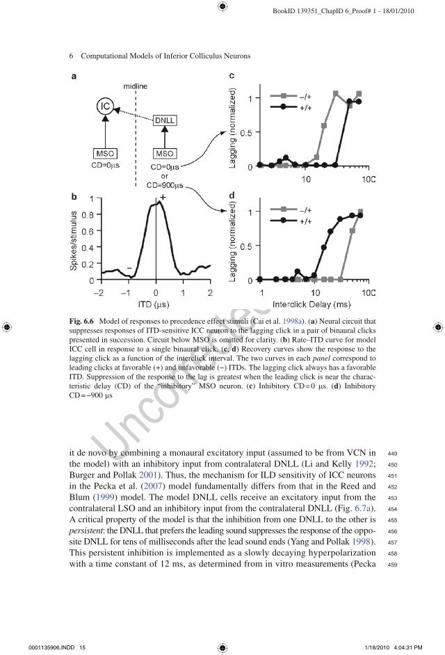
Two computational modeling studies have investigated the mechanisms underlying neural echo suppression in the IC. The model of Cai et al. (1998a) focuses on the binaural response properties of low-frequency ICC neurons that are sensitive to ITDs. The model incorporates a model of auditory nerve fibers (Carney 1993), models of VCN spherical and globular bushy cells (Rothman et al. 1993), and a model of MSO cells (Brughera et al. 1996). The ICC model neuron is excited by an ipsilateral MSO model neuron and inhibited by a contralateral MSO neuron via an inhibitory interneuron, presumed to be in the DNLL, which is not explicitly mod-eled (Fig. 6.6a). The rate–ITD curve of the model ICC cell for a single binaural click stimulus peaks at the characteristic delay of the ipsilateral MSO input (0 ms, Fig. 6.6b). This response is controlled entirely by the ipsilateral MSO because the contralateral inhibition arrives too late to have an effect with transient stimuli. The effects of the inhibitory input on the ICC cell are relatively long-lasting compared to those of the excitatory input, thus the inhibitory inputs activated by the leading sound suppress the response to the lagging sound over a range of delays. This is illustrated in Fig. 6.6c, d, which plot responses to the lag click as a function of the interclick delay. The lag click is held at the best ITD, while the lead click is either at the best (+) or worst (−) ITD. If the excitatory and inhibitory MSO cells have the same best ITD, then the response of the model ICC neuron to the lagging sound is most strongly suppressed for a leading stimulus at the best ITD of the ICC cell (Fig. 6.6c). If, on the other hand, the best ITD of the inhibitory MSO cell is set at the worst ITD of the excitatory MSO neuron, then a leading stimulus at the worst ITD of the ICC cell creates the maximum suppression (Fig. 6.6d).
The model of Pecka et al. (2007) simulates a different (and much smaller) population of ICC neurons for which the response to a lagging stimulus is enhanced when the lead stimulus arises from a favorable location (Burger and Pollak 2001). Experiments in which DNLL activity is blocked pharmacologically suggest that these ICC neurons do not inherit their ILD sensitivity from the LSO, but rather create
0001135906.INDD 14 1/18/2010 4:04:30 PM
404
405
406
407
408
409
410
411
412
413
414
415
416
417
418
419
420
421
422
423
424
425
426
427
428
429
430
431
432
433
434
435
436
437
438
439
440
441
442
443
444
445
446
447
448
BookID 139351_ChapID 6_Proof# 1 - 18/01/2010
6 Computational Models of Inferior Colliculus Neurons
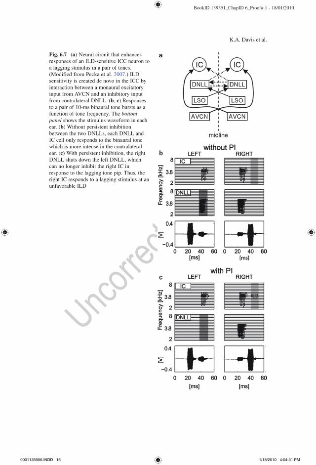
it de novo by combining a monaural excitatory input (assumed to be from VCN in the model) with an inhibitory input from contralateral DNLL (Li and Kelly 1992; Burger and Pollak 2001). Thus, the mechanism for ILD sensitivity of ICC neurons in the Pecka et al. (2007) model fundamentally differs from that in the Reed and Blum (1999) model. The model DNLL cells receive an excitatory input from the contralateral LSO and an inhibitory input from the contralateral DNLL (Fig. 6.7a). A critical property of the model is that the inhibition from one DNLL to the other is persistent: the DNLL that prefers the leading sound suppresses the response of the oppo-site DNLL for tens of milliseconds after the lead sound ends (Yang and Pollak 1998). This persistent inhibition is implemented as a slowly decaying hyperpolarization with a time constant of 12 ms, as determined from in vitro measurements (Pecka
Fig. 6.6 Model of responses to precedence effect stimuli (Cai et al. 1998a). (a) Neural circuit that suppresses responses of ITD-sensitive ICC neuron to the lagging click in a pair of binaural clicks presented in succession. Circuit below MSO is omitted for clarity. (b) Rate–ITD curve for model ICC cell in response to a single binaural click. (c, d) Recovery curves show the response to the lagging click as a function of the interclick interval. The two curves in each panel correspond to leading clicks at favorable (+) and unfavorable (−) ITDs. The lagging click always has a favorable ITD. Suppression of the response to the lag is greatest when the leading click is near the charac-teristic delay (CD) of the “inhibitory” MSO neuron. (c) Inhibitory CD = 0 ms. (d) Inhibitory CD = −900 ms
0001135906.INDD 15 1/18/2010 4:04:31 PM
449
450
451
452
453
454
455
456
457
458
459
BookID 139351_ChapID 6_Proof# 1 - 18/01/2010
K.A. Davis et al.
Fig. 6.7 (a) Neural circuit that enhances responses of an ILD-sensitive ICC neuron to a lagging stimulus in a pair of tones. (Modified from Pecka et al. 2007.) ILD sensitivity is created de novo in the ICC by interaction between a monaural excitatory input from AVCN and an inhibitory input from contralateral DNLL. (b, c) Responses to a pair of 10-ms binaural tone bursts as a function of tone frequency. The bottom panel shows the stimulus waveform in each ear. (b) Without persistent inhibition between the two DNLLs, each DNLL and IC cell only responds to the binaural tone which is more intense in the contralateral ear. (c) With persistent inhibition, the right DNLL shuts down the left DNLL, which can no longer inhibit the right IC in response to the lagging tone pip. Thus, the right IC responds to a lagging stimulus at an unfavorable ILD
0001135906.INDD 16 1/18/2010 4:04:31 PM
BookID 139351_ChapID 6_Proof# 1 - 18/01/2010
6 Computational Models of Inferior Colliculus Neurons
et al. 2007). Figure 6.7b, c show responses of the DNLL and ICC model cells that demonstrate the effect of persistent inhibition. The stimulus is a pair of 10-ms binaural tone bursts such that the first ILD favors the left ear, and the second favors the right ear. Without persistent inhibition (Fig. 6.7b), the right DNLL and ICC cells are excited by the leading sound, while the left DNLL and ICC cells are excited by the lag. With inhibition, however, the left DNLL is persistently inhibited by the lead sound in the left ear, so that it cannot inhibit the response of the right ICC to the lagging sound (Fig. 6.7c). Therefore, ICC cell responses to the lagging sound depend on the ILD of the leading sound for a range of delays between the two sounds. In particular, persistent inhibition evoked by the lead stimulus causes an ICC cell to respond to a lagging stimulus to which it would not respond if presented in isolation. This altered neural representation of the lagging sound may partially underlie the poor localization of trailing sounds by human listeners, which is a characteristic of the PE (Zurek 1987).
Persistent inhibition arising from the DNLL is a common element of the models of Cai et al. (1998a) and Pecka et al. (2007), but the models diverge in other respects. In the Cai et al. model inhibition occurs in the ICC, where it directly inhibits the response to a lagging sound. In the Pecka et al. model, the persistent inhibi-tion occurs between the two DNLLs and disinhibits the IC response to the lagging sound. The Cai et al. model focuses on the ITD-sensitive pathway while Pecka et al. are concerned with ILD-sensitive responses. Such differences highlight the fact that the PE is not a unitary phenomenon and is not likely to be mediated by a single neural mechanism. Moreover, the relationship between neural echo suppression observed with a simple lead-lag pair and the practical challenge of hearing in rever-berant environments comprising a large number of reflections is not clear (Devore et al. 2009). Exploration of these models using realistic reverberant stimuli is an important next step. Another important task is to clearly distinguish the contributions of peripheral and central mechanisms to neural echo suppression phenomena in the ICC (Hartung and Trahiotis 2001). Finally, it will be important to develop neural population models to explore the psychophysical consequences of echo suppression, not only for the PE, but also for other phenomena such as forward masking and sensitivity to motion cues (Xia et al. 2009).
6.4 Localization of a Moving Sound Source
In everyday listening environments, the acoustic cues for sound localization often vary over time as a result of the motion of a sound source relative to the listener’s head. Several psychophysical (Grantham 1998; Dong et al. 2000) and neuroimaging (Griffiths et al. 1998) studies suggest there may exist specialized detectors and brain regions that are selectively activated by sound motion cues such as time-varying interaural phase differences (IPDs). However, other studies have concluded that the auditory system responds sluggishly to changing localization cues and that acoustic motion generally impairs the accuracy of sound localization (e.g., Grantham and
0001135906.INDD 17 1/18/2010 4:04:31 PM
460
461
462
463
464
465
466
467
468
469
470
471
472
473
474
475
476
477
478
479
480
481
482
483
484
485
486
487
488
489
490
491
492
493
494
495
496
497
498
499
500
BookID 139351_ChapID 6_Proof# 1 - 18/01/2010
K.A. Davis et al.
Wightman 1978). The two points of view are not mutually exclusive as there could be specialized detectors that detect motion regardless of the instantaneous location of the sound source.
Studies of neuronal sensitivity to temporal variations in IPD suggest that a major transformation in the coding of this motion cue occurs between the SOC and the IC. Neurons in the MSO, where IPD is initially encoded, are generally insensitive to motion cues (Spitzer and Semple 1998). That is, the responses of MSO neurons to time-varying IPD stimuli resemble their responses to static IPD stimuli for each time instant, that is, these neurons track the instantaneous IPD (dashed line, Fig. 6.2e). In contrast, many low-frequency neurons in the ICC are sensitive to dynamic changes in IPD (Spitzer and Semple 1993, 1998; McAlpine and Palmer 2002). As shown in Fig. 6.2e (solid lines), the responses of ICC neurons to dynamic stimuli swept across complementary narrow ranges of IPDs are not continuous with each other, although the entire set of partial response profiles tends to follow the general shape of the static IPD function measured over a wide IPD range. The responses to dynamic IPD arcs are always steeper than the static IPD function, with motion toward the peak of the static function resulting in overshoot and motion away from the peak resulting in undershoot. Over a restricted range of IPDs, responses to opposite directions of motion thus form hysteresis loops (gray shaded areas). Importantly, dynamic IPD stimuli can evoke a strong excitatory response for instantaneous IPDs for which there is no response to static IPDs (asterisk), a phenomenon that has been termed “rise-from-nowhere.”
The difference between the responses of ICC and MSO neurons to dynamic IPD stimuli suggests that sensitivity to sound-motion cues emerges at the level of the ICC. One explanation for sensitivity to motion cues is a nonlinear interaction between IPD-tuned excitatory and inhibitory inputs to ICC (Spitzer and Semple 1998). Alternatively, motion sensitivity could reflect “adaptation of excitation” (Spitzer and Semple 1998; McAlpine et al. 2000), in which the firing rates of ICC neurons depend on both the instantaneous value of IPD and their recent firing history (not the history of the IPD cues per se). In support of the adaptation hypothesis over the inhibition hypothesis, McAlpine and Palmer (2002) found that sensitivity to apparent motion cues in ICC is actually decreased by the inhibitory transmitter g-aminobutyric acid (GABA) and increased by the GABA-antagonist bicuculline.
The roles of adaptation and inhibition in shaping ICC unit sensitivity to motion cues have been examined in two computational modeling studies (Cai et al. 1998a, b; Borisyuk et al. 2001, 2002). Both support the proposal that the primary mechanism responsible for sensitivity to motion cues is adaptation-of-excitation. Cai et al. (1998a) first tested their model ICC cell discussed in Sect. 6.3, which receives IPD-tuned excitatory and inhibitory inputs from the ipsilateral and contralateral MSO, respectively. They found that this model version does not produce differential responses to stimuli with dynamic and static IPDs. Subsequently, they added an adaptation mechanism that causes the model to exhibit sharpened dynamic IPD tuning, and sensitivity to the direction of IPD change (hysteresis). The adaptation mechanism in their model is a calcium-activated potassium channel. After each spike of the ICC cell, the conductance of this channel increases by a small amount,
0001135906.INDD 18 1/18/2010 4:04:31 PM
501
502
503
504
505
506
507
508
509
510
511
512
513
514
515
516
517
518
519
520
521
522
523
524
525
526
527
528
529
530
531
532
533
534
535
536
537
538
539
540
541
542
543
544
545
BookID 139351_ChapID 6_Proof# 1 - 18/01/2010
6 Computational Models of Inferior Colliculus Neurons
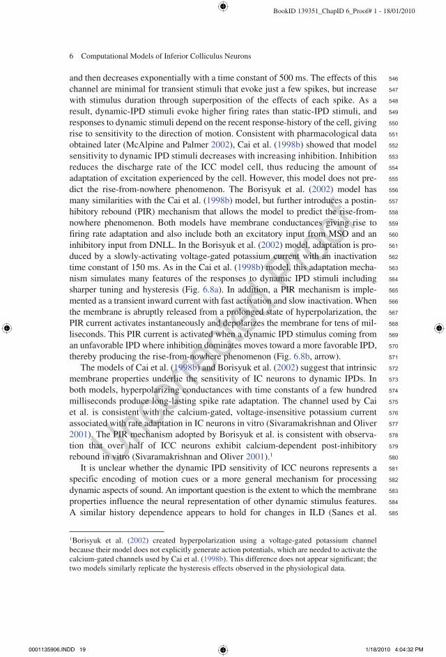
and then decreases exponentially with a time constant of 500 ms. The effects of this channel are minimal for transient stimuli that evoke just a few spikes, but increase with stimulus duration through superposition of the effects of each spike. As a result, dynamic-IPD stimuli evoke higher firing rates than static-IPD stimuli, and responses to dynamic stimuli depend on the recent response-history of the cell, giving rise to sensitivity to the direction of motion. Consistent with pharmacological data obtained later (McAlpine and Palmer 2002), Cai et al. (1998b) showed that model sensitivity to dynamic IPD stimuli decreases with increasing inhibition. Inhibition reduces the discharge rate of the ICC model cell, thus reducing the amount of adaptation of excitation experienced by the cell. However, this model does not pre-dict the rise-from-nowhere phenomenon. The Borisyuk et al. (2002) model has many similarities with the Cai et al. (1998b) model, but further introduces a postin-hibitory rebound (PIR) mechanism that allows the model to predict the rise-from-nowhere phenomenon. Both models have membrane conductances giving rise to firing rate adaptation and also include both an excitatory input from MSO and an inhibitory input from DNLL. In the Borisyuk et al. (2002) model, adaptation is pro-duced by a slowly-activating voltage-gated potassium current with an inactivation time constant of 150 ms. As in the Cai et al. (1998b) model, this adaptation mecha-nism simulates many features of the responses to dynamic IPD stimuli including sharper tuning and hysteresis (Fig. 6.8a). In addition, a PIR mechanism is imple-mented as a transient inward current with fast activation and slow inactivation. When the membrane is abruptly released from a prolonged state of hyperpolarization, the PIR current activates instantaneously and depolarizes the membrane for tens of mil-liseconds. This PIR current is activated when a dynamic IPD stimulus coming from an unfavorable IPD where inhibition dominates moves toward a more favorable IPD, thereby producing the rise-from-nowhere phenomenon (Fig. 6.8b, arrow).
The models of Cai et al. (1998b) and Borisyuk et al. (2002) suggest that intrinsic membrane properties underlie the sensitivity of IC neurons to dynamic IPDs. In both models, hyperpolarizing conductances with time constants of a few hundred milliseconds produce long-lasting spike rate adaptation. The channel used by Cai et al. is consistent with the calcium-gated, voltage-insensitive potassium current associated with rate adaptation in IC neurons in vitro (Sivaramakrishnan and Oliver 2001). The PIR mechanism adopted by Borisyuk et al. is consistent with observa-tion that over half of ICC neurons exhibit calcium-dependent post-inhibitory rebound in vitro (Sivaramakrishnan and Oliver 2001).1
It is unclear whether the dynamic IPD sensitivity of ICC neurons represents a specific encoding of motion cues or a more general mechanism for processing dynamic aspects of sound. An important question is the extent to which the membrane properties influence the neural representation of other dynamic stimulus features. A similar history dependence appears to hold for changes in ILD (Sanes et al.
1 Borisyuk et al. (2002) created hyperpolarization using a voltage-gated potassium channel because their model does not explicitly generate action potentials, which are needed to activate the calcium-gated channels used by Cai et al. (1998b). This difference does not appear significant; the two models similarly replicate the hysteresis effects observed in the physiological data.
0001135906.INDD 19 1/18/2010 4:04:32 PM
546
547
548
549
550
551
552
553
554
555
556
557
558
559
560
561
562
563
564
565
566
567
568
569
570
571
572
573
574
575
576
577
578
579
580
581
582
583
584
585

BookID 139351_ChapID 6_Proof# 1 - 18/01/2010
K.A. Davis et al.
1998). However, most of the models described in other sections of this chapter consider only either static or brief stimuli that would minimally activate the conduc-tances used by Cai et al. and Borisyuk et al. An exception is amplitude modulated (AM) stimuli; yet surprisingly, none of the proposed models for AM tuning in ICC (Sect. 6.6) considers intrinsic membrane channels as a possible mechanism. The slow adaptive effects described in this section may also contribute to PE phenomena evoked with long-duration stimuli, but this has yet to be explored.
6.5 Population Models of ITD Processing
The coincidence detection mechanism that underlies ITD encoding in the MSO can be viewed over long time scales as a cross-correlation of the inputs from the two ears after taking into account cochlear filtering (Yin and Chan 1990). Rate responses of ITD-sensitive ICC neurons to simple low-frequency binaural stimuli are quantitatively consistent with a cross-correlation operation (Yin et al. 1987; Devore et al. 2009). More complex stimuli encountered in everyday acoustic environments, however,
Fig. 6.8 Model of responses to stimuli with time-varying IPD (Borisyuk et al. 2002). (a) Rate–IPD curves for model ICC cell with a membrane channel producing strong spike rate adaptation. Response to static stimuli (thick solid line) is superimposed on responses to three different dynamic stimuli swept over different ranges of IPD. Arrows at the top indicate the sweep ranges. Dashed lines correspond to sweeps toward negative IPDs, thin solid lines sweeps toward positive IPDs. Rate adaptation is responsible for the hysteresis in the responses to dynamic IPD stimuli. (b) Rate–IPD curves for model IC cell with an additional channel producing postinhibitory rebound (PIR). With PIR channel, model produces “rise-from-nowhere” (arrow)
0001135906.INDD 20 1/18/2010 4:04:32 PM
586
587
588
589
590
591
592
593
594
595
596
597
598
599

BookID 139351_ChapID 6_Proof# 1 - 18/01/2010
6 Computational Models of Inferior Colliculus Neurons
reveal discrepancies between IC behavior and this model. Responses in cat ICC show greater sensitivity to ITD in the presence of reverberation than predicted by long-term cross-correlation (Devore et al. 2009). Similarly, ITD sensitivity in the external nucleus of the inferior colliculus (ICX) of the barn owl is more robust to noise than the model predicts (Keller and Takahashi 1996). Such observations suggest that specialized processing may occur in the IC to maintain the potency of spatial cues in the presence of degrading influences.
6.5.1 Robust Coding of ITD in Noise in Barn Owl IC
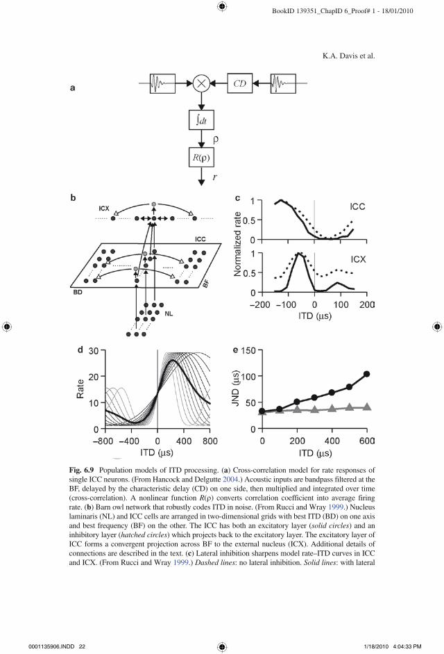
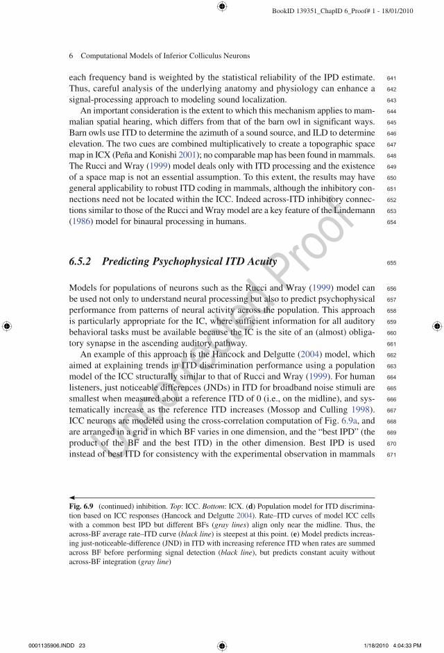
Rucci and Wray (1999) used a model to investigate the role of IC intrinsic circuitry in creating robust ITD coding in noise in the barn owl ICX. The ICX in this species contains a map of auditory space where neurons are broadly tuned to frequency, but sharply tuned to both ITD and ILD (which is primarily an elevation cue in the barn owl due to the asymmetry of the external ears). The ICX receives inputs from ICC where neurons are sharply tuned to both frequency and ITD. The model comprises two layers of ICC neurons, one excitatory and one inhibitory (Fig. 6.9b). Each layer is a grid with best ITD systematically varied in one dimension and best frequency (BF) varied in the other. The input to the ICC comes from the ipsilateral nucleus laminaris (NL, the avian homolog of MSO), where cells are arranged in a corre-sponding grid making point-to-point (i.e., topographic) connections to the excitatory layer in ICC. Each NL neuron is modeled by bandpass filtering the acoustic inputs around the BF to approximate cochlear processing, delaying the filter output on one side by the best delay, and multiplying and integrating (i.e., cross-correlating) the filter outputs from the two sides (Fig. 6.9a). A memoryless nonlinear function con-verts the resulting correlation value into a firing rate. The excitatory layer in ICC is topographically connected to the inhibitory layer. Specifically, each cell in the inhibitory layer receives input from one excitatory-layer neuron with the same BF and best ITD, and projects back to all excitatory cells having the same BF but different best ITDs (i.e., the inhibition is lateral but not recurrent). The ICX model is a one-dimensional array of neurons organized by best ITD. Each ICX cell receives con-vergent input from all excitatory ICC cells that have the same best ITD, regardless of BF. The ICX also contains its own lateral inhibitory connections.
The results show that sharp ITD tuning is maintained in ICX in the presence of noise only when the lateral connections are included. The stimulus was a broadband target sound contaminated by a band of uncorrelated noise. Figure 6.9c plots model rate–ITD curves with and without the lateral inhibitory connections, and shows that the lateral inhibition across BD sharpens tuning in ICC and, especially, ICX without altering the best ITD. From the perspective of a single model neuron, the sharpening due to lateral inhibition is relatively modest, but when pooled across the entire population, the improvement of ITD coding in noise is substantial. Rucci and Wray further demonstrate that lateral inhibition and convergence across BF effectively implement a generalized cross-correlation, in which the cross-correlation function in
0001135906.INDD 21 1/18/2010 4:04:32 PM
600
601
602
603
604
605
606
607
608
609
610
611
612
613
614
615
616
617
618
619
620
621
622
623
624
625
626
627
628
629
630
631
632
633
634
635
636
637
638
639
640
BookID 139351_ChapID 6_Proof# 1 - 18/01/2010
K.A. Davis et al.
Fig. 6.9 Population models of ITD processing. (a) Cross-correlation model for rate responses of single ICC neurons. (From Hancock and Delgutte 2004.) Acoustic inputs are bandpass filtered at the BF, delayed by the characteristic delay (CD) on one side, then multiplied and integrated over time (cross-correlation). A nonlinear function R(r) converts correlation coefficient into average firing rate. (b) Barn owl network that robustly codes ITD in noise. (From Rucci and Wray 1999.) Nucleus laminaris (NL) and ICC cells are arranged in two-dimensional grids with best ITD (BD) on one axis and best frequency (BF) on the other. The ICC has both an excitatory layer (solid circles) and an inhibitory layer (hatched circles) which projects back to the excitatory layer. The excitatory layer of ICC forms a convergent projection across BF to the external nucleus (ICX). Additional details of connections are described in the text. (c) Lateral inhibition sharpens model rate–ITD curves in ICC and ICX. (From Rucci and Wray 1999.) Dashed lines: no lateral inhibition. Solid lines: with lateral
0001135906.INDD 22 1/18/2010 4:04:33 PM
BookID 139351_ChapID 6_Proof# 1 - 18/01/2010
6 Computational Models of Inferior Colliculus Neurons
each frequency band is weighted by the statistical reliability of the IPD estimate. Thus, careful analysis of the underlying anatomy and physiology can enhance a signal-processing approach to modeling sound localization.
An important consideration is the extent to which this mechanism applies to mam-malian spatial hearing, which differs from that of the barn owl in significant ways. Barn owls use ITD to determine the azimuth of a sound source, and ILD to determine elevation. The two cues are combined multiplicatively to create a topographic space map in ICX (Peña and Konishi 2001); no comparable map has been found in mammals. The Rucci and Wray (1999) model deals only with ITD processing and the existence of a space map is not an essential assumption. To this extent, the results may have general applicability to robust ITD coding in mammals, although the inhibitory con-nections need not be located within the ICC. Indeed across-ITD inhibitory connec-tions similar to those of the Rucci and Wray model are a key feature of the Lindemann (1986) model for binaural processing in humans.
6.5.2 Predicting Psychophysical ITD Acuity
Models for populations of neurons such as the Rucci and Wray (1999) model can be used not only to understand neural processing but also to predict psychophysical performance from patterns of neural activity across the population. This approach is particularly appropriate for the IC, where sufficient information for all auditory behavioral tasks must be available because the IC is the site of an (almost) obliga-tory synapse in the ascending auditory pathway.
An example of this approach is the Hancock and Delgutte (2004) model, which aimed at explaining trends in ITD discrimination performance using a population model of the ICC structurally similar to that of Rucci and Wray (1999). For human listeners, just noticeable differences (JNDs) in ITD for broadband noise stimuli are smallest when measured about a reference ITD of 0 (i.e., on the midline), and sys-tematically increase as the reference ITD increases (Mossop and Culling 1998). ICC neurons are modeled using the cross-correlation computation of Fig. 6.9a, and are arranged in a grid in which BF varies in one dimension, and the “best IPD” (the product of the BF and the best ITD) in the other dimension. Best IPD is used instead of best ITD for consistency with the experimental observation in mammals
Fig. 6.9 (continued) inhibition. Top: ICC. Bottom: ICX. (d) Population model for ITD discrimina-tion based on ICC responses (Hancock and Delgutte 2004). Rate–ITD curves of model ICC cells with a common best IPD but different BFs (gray lines) align only near the midline. Thus, the across-BF average rate–ITD curve (black line) is steepest at this point. (e) Model predicts increas-ing just-noticeable-difference (JND) in ITD with increasing reference ITD when rates are summed across BF before performing signal detection (black line), but predicts constant acuity without across-BF integration (gray line)
0001135906.INDD 23 1/18/2010 4:04:33 PM
641
642
643
644
645
646
647
648
649
650
651
652
653
654
655
656
657
658
659
660
661
662
663
664
665
666
667
668
669
670
671
BookID 139351_ChapID 6_Proof# 1 - 18/01/2010
K.A. Davis et al.
that best IPD and BF are more nearly orthogonal than best ITD and BF (McAlpine et al. 2001; Hancock and Delgutte 2004). Unlike the models considered so far, the Hancock and Delgutte model explicitly models the internal noise resulting from variability in firing rates in order to compute the expected performance for an ideal observer of the population neural activity. ITD JNDs are computed using standard signal detection techniques (Green and Swets 1988) from patterns of model firing rates evoked by pairs of stimuli with different ITDs. Figure 6.9e compares model-generated ITD JNDs to psychophysical data (Mossop and Culling 1998) as a function of reference ITD. The model predicts the degradation in ITD acuity with increasing reference ITD when information is pooled across BF (black line), but predicts con-stant ITD acuity when there is no across-BF convergence (gray line). This property occurs because the slopes of rate–ITD curves tend to align across BF near the mid-line, but not for more lateral locations (Fig. 6.9d) (McAlpine et al. 2001). Consequently, convergence across BF reinforces sensitivity to changes in ITD near the midline, but blurs it more laterally. An extension of this model (Hancock 2007) predicts the later-alization of stimuli with independently applied interaural time and phase shifts (Stern et al. 1988).
Convergence across BF is an important element of both the Rucci and Wray (1999) and Hancock and Delgutte (2004) models and is also a feature of some func-tional models for predicting human binaural performance (Stern et al. 1988; Shackleton et al. 1992). Together, the results from the IC models suggest that pooling of information across BF helps create a robust neural ITD code on the midline at the expense of ITD acuity on the periphery. The Hancock and Delgutte (2004) model considered only single sound sources in anechoic space and hence did not need the lateral inhibitory connections of Rucci and Wray (1999). Application of the model in the presence of competing sources or reverberation may require such connections.
6.6 Sensitivity to Amplitude Modulation
Many natural sounds contain prominent fluctuations in their amplitude envelope (Singh and Theunissen 2003). Amplitude modulation (AM) information is used by the auditory system in a variety of tasks, including speech perception (Steeneken and Houtgast 1980; Rosen 1992), pitch perception (Plack and Oxenham 2005) and auditory scene analysis (Darwin and Carlyon 1995). Envelope information appears to be primarily encoded in the temporal response patterns of neurons in the early stages of the auditory system, and then partly transformed into a rate-based code at higher stages of processing (Joris et al. 2004).
Neural responses to AM stimuli, most often sinusoidally amplitude-modulated (SAM) tones, are typically quantified based on average firing rate and synchrony to the modulation period. These metrics are plotted against modulation frequency to obtain rate and temporal modulation transfer functions (MTFs), respectively. A temporal MTF has both a magnitude (the modulation gain) and a phase representing the delay
0001135906.INDD 24 1/18/2010 4:04:33 PM
672
673
674
675
676
677
678
679
680
681
682
683
684
685
686
687
688
689
690
691
692
693
694
695
696
697
698
699
700
701
702
703
704
705
706
707
708
709
710
711
BookID 139351_ChapID 6_Proof# 1 - 18/01/2010
6 Computational Models of Inferior Colliculus Neurons
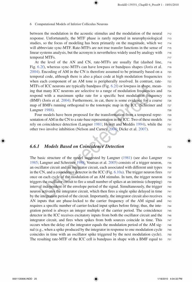
between the modulation in the acoustic stimulus and the modulation of the neural response. Unfortunately, the MTF phase is rarely reported in neurophysiological studies, so the focus of modeling has been primarily on the magnitude, which we will abbreviate sync-MTF. Rate-MTFs are not true transfer functions in the sense of linear systems analysis, but the acronym is nevertheless widely used by analogy with temporal MTFs.
At the level of the AN and CN, rate-MTFs are usually flat (dashed line, Fig. 6.2f), whereas sync-MTFs can have lowpass or bandpass shapes (Joris et al. 2004). Encoding of AM in the CN is therefore assumed to be primarily based on a temporal code, although there is also a place code at high modulation frequencies when each component of an AM tone is peripherally resolved. In contrast, rate-MTFs of ICC neurons are typically bandpass (Fig. 6.2f) or lowpass in shape, mean-ing that many ICC neurons are selective to a range of modulation frequencies and respond with a maximum spike rate for a specific best modulation frequency (BMF) (Joris et al. 2004). Furthermore, in cat, there is some evidence for a coarse map of BMFs running orthogonal to the tonotopic map in the ICC (Schreiner and Langner 1988).
Four models have been proposed for the transformation from a temporal repre-sentation of AM in the CN to a rate-base representation in the ICC. Two of these models rely on coincidence detection (Langner 1981; Hewitt and Meddis 1994), while the other two involve inhibition (Nelson and Carney 2004; Dicke et al. 2007).
6.6.1 Models Based on Coincidence Detection
The basic structure of the model suggested by Langner (1981) (see also Langner 1985; Langner and Schreiner 1988; Voutsas et al. 2005) consists of a trigger neuron, an oscillator circuit and an integrator circuit, each associated with different unit types in the CN, and a coincidence detector in the ICC (Fig. 6.10a). The trigger neuron fires once on each cycle of the modulation of an AM stimulus. In turn, the trigger neuron triggers the oscillator circuit to fire a small number of spikes at an intrinsic (chopping) interval independent of the envelope period of the signal. Simultaneously, the trigger neuron activates the integrator circuit, which then fires a single spike delayed in time by the integration period of the circuit. Importantly, the integrator circuit also receives AN inputs that are phase-locked to the carrier frequency of the AM signal and requires a specific number of carrier-locked input spikes before firing; thus, the inte-gration period is always an integer multiple of the carrier period. The coincidence detector in the ICC receives excitatory inputs from both the oscillator circuit and the integrator circuit, and fires when spikes from both sources coincide in time. This occurs when the delay of the integrator equals the modulation period of the AM sig-nal (e.g., when a spike produced by the integrator in response to one modulation cycle coincides in time with an oscillator spike triggered by the next modulation cycle). The resulting rate-MTF of the ICC cell is bandpass in shape with a BMF equal to
0001135906.INDD 25 1/18/2010 4:04:33 PM
712
713
714
715
716
717
718
719
720
721
722
723
724
725
726
727
728
729
730
731
732
733
734
735
736
737
738
739
740
741
742
743
744
745
746
747
748
749
750
751

BookID 139351_ChapID 6_Proof# 1 - 18/01/2010
Fig. 6.10 Models for rate tuning to modulation frequency based on coincidence detection. (a) Block diagram of the Langner (1981) model. (From Voutsas et al. 2005.) The trigger neuron located in the CN receives inputs from the auditory nerve (AN) and produces one spike per modulation cycle t
m
of an AM tone. This neuron triggers both an oscillator circuit and an integrator circuit. The oscillator fires a small number k of spikes at regular intervals t
k in response to the trigger. The integrator circuit
receives inputs phase locked to the carrier frequency of the AM stimulus from the AN and fires one spike a predetermined number n of carrier cycles t
c after each trigger. The coincidence detector
located in ICC fires when it receives simultaneous spikes from the integrator and oscillator circuits, thereby converting a temporal code for periodicity into a rate code. The coincidence detector neuron has a bandpass rate MTF, with a BMF approximately equal to 1/nt
c. The circuit as a whole imple-
ments the “coincidence” or “periodicity” equation (bottom right) which accounts for the pitch shift of harmonic complex tones. (b) Block diagram of the Hewitt and Meddis (1994) model for rate tuning to AM in ICC. Auditory nerve fibers innervating a given cochlear place project to an array of chopper neurons in VCN that show bandpass temporal MTFs and differ in their best modulation frequency (BMF). A set of chopper neurons having the same BMF projects to one coincidence detector neuron in ICC, endowing this neuron with a bandpass rate MTF. Coincidence detection converts a temporal code for AM in the VCN into a rate code in the IC
0001135906.INDD 26 1/18/2010 4:04:34 PM
BookID 139351_ChapID 6_Proof# 1 - 18/01/2010
6 Computational Models of Inferior Colliculus Neurons
the inverse of the integration period of the integrator.2 A key prediction of this model is that the BMF period must be linearly related to the stimulus carrier period (the so-called “periodicity” or “coincidence” equation; see Fig. 6.10a). While such a linear relationship holds approximately for some IC neurons in both cat (Langner and Schreiner 1988) and guinea fowl (Langner 1983), it does not appear to hold in general (Krishna and Semple 2000). An additional drawback is that the model only works at low carrier frequencies (<5 kHz), where the input to the integrator circuit input retains synchrony to the carrier. Thus, another mechanism is required to explain results at higher carrier frequencies despite the basic similarity of rate-MTF shapes throughout the tonotopic axis of the ICC.
The second coincidence detector model for the formation of bandpass AM tuning in the ICC (Hewitt and Meddis 1994) is based on an array of VCN chopper cells that fire spikes at fairly regular intervals in response to AM tones (Fig. 6.10b). The chopping rate of these model choppers (Hewitt et al. 1992) is typically unrelated to either the carrier or the modulation frequency of the AM stimulus, that is, their rate-MTFs are flat. Importantly, with unmodulated stimuli, two chopper units with the same chopping rate gradually lose temporal synchrony with one another over time because of random fluctuations in their interspike intervals. On the other hand, when the intrinsic chop-ping rate of a group of VCN chopper cells matches the modulation frequency of an AM stimulus, then the chopper cells remains tightly synchronized to the AM stimulus and to each other throughout the stimulus duration. Thus, chopper units exhibit bandpass sync-MTFs with BMFs equal to their intrinsic chopping rate. The BMF is controlled by adjusting the strength of a K+ membrane conductance in the chopper model neuron (Hewitt et al. 1992). A group of VCN chopper units with the same intrinsic chopping rate converge onto an ICC cell acting as a coincidence detector, that is, the ICC cell fires only when it receives a sufficient number of synchronous VCN inputs. Such coincidences are most likely to occur when the modulation fre-quency of the stimulus matches the chopping rate of the VCN inputs. The Hewitt and Meddis (1994) model therefore transforms the bandpass sync-MTFs of VCN chopper units into bandpass rate-MTFs in the ICC. This transformation from a temporal code to a rate code is achieved under the strong constraint that all the VCN inputs to a given ICC cell have identical chopping rates. Guerin et al. (2006) found that if this constraint is relaxed, then the model ICC cell still exhibits a band-pass shaped rate-MTF but the sync-MTF becomes more noisy and less bandpass in shape than those of real ICC units. The strength of the synchronous response can be enhanced by adding a second layer of coincidence detectors in the ICC.
The Langner (1981) and Hewitt and Meddis (1994) models have several circuit elements in common. Both use coincidence detectors located in ICC to transform a temporal code for modulation frequency into a rate code, and both include oscillator
2 One problem with this model structure is that the ICC cell responds equally well to harmonics of the BMF as to the BMF itself. Voutsas et al. (2005) avoid this problem by having the trigger neuron inhibit the ICC cell, via an interneuron putatively located in the VNLL, for a predefined period of time equal to at least one-half of the integration period.
0001135906.INDD 27 1/18/2010 4:04:34 PM
752
753
754
755
756
757
758
759
760
761
762
763
764
765
766
767
768
769
770
771
772
773
774
775
776
777
778
779
780
781
782
783
784
785
786
787
788
789
790

BookID 139351_ChapID 6_Proof# 1 - 18/01/2010
K.A. Davis et al.
neurons (choppers) putatively located in the CN. However, whereas bandpass AM tuning in the Hewitt and Meddis model is inherited from the tuning of the VCN chopper neurons, it is controlled by the integration time of the integrator circuit in the Langner model. One outstanding issue for both models is the disparity in the ranges of VCN chopper cell synchrony BMFs (150–700 Hz; (Frisina et al. 1990; Rhode and Greenberg 1994) and ICC unit rate BMFs (1–150 Hz; Krishna and Semple 2000).3 Moreover, intracellular recordings from ICC neurons with bandpass rate-MTFs fail to show strong stimulus-locked modulations of the membrane potential when the modulation frequency of an AM tone stimulus matches the BMF, posing a challenge to the idea that these cells act as coincidence detectors (Geis and Borst 2009).
6.6.2 Models Based on Inhibition
Nelson and Carney (2004) proposed a model for bandpass rate tuning to AM that differs from the models discussed in the preceding text in that it relies on interaction between excitation and inhibition rather than coincidence detection to produce tuning. In this model, ICC cells receive same-BF inhibitory and excitatory (SFIE) input from a VCN bushy cell which, in turn, receives SFIE input from auditory nerve fibers (Fig. 6.11a). Both excitation and inhibition are phase locked to each modulation cycle, but with different delays. At the VCN level, the excitatory inputs are stronger and faster than the inhibitory inputs. As a result, the bushy cell’s response to SAM tones largely resembles that of its AN inputs: that is, the bushy cell has a flat rate-MTF and a lowpass sync-MTF (Fig. 6.11b). In contrast, at the level of the ICC, the inhibitory inputs are stronger (but still slower) than the excitatory
Fig. 6.11 Models for rate tuning to modulation in ICC based on inhibition. (a) Block diagram of the Nelson and Carney (2004) model. An ICC model neuron receives both a fast excitatory input and a delayed inhibitory input from model VCN neurons having the same BF. The VCN model neuron receives structurally similar excitatory and inhibitory inputs from the AN. (b) Typical rate-MTFs and sync-MTFs for AN, VCN and ICC model neurons. (From Nelson and Carney 2004.) (c) Block diagram of the Dicke et al. (2007) model. The model includes two neuron types in VCN: entraining (EN) neurons similar to octopus cells with rate MTFs linearly increasing up to 800 Hz, and constant-rate (CR) neurons with flat rate MTFs. Lowpass (LP) neurons in ICC receive excitatory inputs from an adjustable number of CR neurons and an inhibitory input from one EN neuron, giving them a lowpass rate MTF whose cutoff increases with the number of CR inputs. Bandpass (BP) neurons in ICC (BP) receive an excitatory input from one LP neuron and an inhibitory neuron from another LP neuron with a slightly lower cutoff frequency, giving them bandpass rate MTFs. (d) Rate MTFs of the four neuron types in the Dicke et al. (2007) model
3 Studies in both anesthetized cat (Langner and Schreiner 1988) and awake chinchilla (Langner et al. 2002) have reported IC units with rate-BMFs as high at 1,000 Hz, but most of these were multi-units (as opposed to single units) and could be recordings from axons of incoming lemniscal inputs rather than from cell bodies of ICC neurons (see Joris et al. 2004 for discussion).
0001135906.INDD 28 1/18/2010 4:04:34 PM
791
792
793
794
795
796
797
798
799
800
801
802
803
804
805
806
807
808
809
810
811
812

BookID 139351_ChapID 6_Proof# 1 - 18/01/2010
6 Computational Models of Inferior Colliculus Neurons
0001135906.INDD 29 1/18/2010 4:04:35 PM

BookID 139351_ChapID 6_Proof# 1 - 18/01/2010
K.A. Davis et al.
inputs. For AM stimuli with low modulation frequencies, excitation and inhibition occur largely in phase, giving rise to a weak rate response in the ICC neuron. For modulation frequencies near the cell’s BMF, the stimulus-locked excitatory peaks line up in time with the “valleys” in the phase-locked inhibition, giving rise to a robust response. At modulation frequencies above the BMF, the inhibition is no longer phase locked (due its slow time constant) and completely blocks the excita-tion. The ICC model cell thus has a bandpass rate-MTF (Fig. 6.11b), with a BMF determined mainly by the time constants of its inhibitory and excitatory inputs: short time constants give rise to high BMFs and long time constants to lower BMFs. Interestingly, the Nelson and Carney (2004) model is the cascade of two structurally identical SFIE circuits, either of which could, by itself, implement the transformation from a synchrony to a rate code. Nonetheless, the model has the advantage of simu-lating physiological data from both VCN and ICC. However, interpretation of the model structure is complicated by the fact that VCN bushy cells do not project directly to the ICC, but rather to LSO and MSO. Neurons in the LSO show lowpass rate-MTFs (Joris and Yin 1998) suggesting that the transformation into a bandpass MTF must occur at a later stage such as the ICC. MSO neurons in the big brown bat show lowpass or all-pass rate-MTFs (Grothe et al. 2001), also suggesting that a major transformation must occur at a later stage.
Dicke et al. (2007) proposed a model for bandpass rate tuning to AM which, like the Nelson and Carney (2004) model uses inhibition, but has a different principle of operation. In this model, ICC cells with bandpass rate-MTFs receive inputs from other ICC cells with lowpass rate-MTFs which, in turn, receive inputs from neurons in the CN (Fig. 6.11c). The CN stage of the model contains two unit types: (1) entraining (EN) neurons, which fire exactly one spike per modulation cycle of SAM stimuli and (2) constant-rate (CR) neurons, which fire a series of regularly spaced spikes at a rate unrelated to the modulation frequency (i.e., the CR neurons are chop-pers and have flat rate-MTFs). The EN model neurons resemble PVCN units with ideal onset (On-I) response patterns to pure tones. Because they entrain to low-frequency AM tones, their rate-MTFs increase linearly with modulation frequency up to an upper limit at about 800 Hz, above which they fire only at the onset of SAM stimuli (Fig. 6.11d). The cells in the first layer of the ICC, called lowpass (LP) units, are excited by a variable number of CR units and inhibited by EN unit activity. These cells exhibit basically lowpass4 rate-MTFs, and their cutoff frequency increases with increasing number of CR inputs (Fig. 6.11d). The bandpass (BP) cells in the second ICC layer receive a strong inhibitory input from one LP unit and weak excitatory input from another LP unit with a slightly higher cutoff frequency. The interaction of excit-atory and inhibitory inputs results in a bandpass rate-MTF, with a BMF between the cutoff frequencies of the two LP units that comprise its inputs (Fig. 6.11d). This model thus exploits the fact that some ICC cells exhibit lowpass rate-MTFs to generate
4 At modulation frequencies above approximately 800 Hz, the EN neurons providing inhibitory inputs to the LP neurons no longer respond in a sustained manner, causing the firing rate of the LP neurons to increase rapidly. Thus, strictly speaking, the LP neurons have band-reject, not lowpass, rate-MTFs.
0001135906.INDD 30 1/18/2010 4:04:35 PM
813
814
815
816
817
818
819
820
821
822
823
824
825
826
827
828
829
830
831
832
833
834
835
836
837
838
839
840
841
842
843
844
845
846
847
848
849
850
851
852
BookID 139351_ChapID 6_Proof# 1 - 18/01/2010
6 Computational Models of Inferior Colliculus Neurons
bandpass rate tuning in the ICC. It is not known whether the orderly lateral inhibition among neighboring cells assumed in the circuit is biologically realistic.
While the timing between excitation and inhibition is critical in the Nelson and Carney (2004) model to create bandpass rate tuning to AM, the Dicke et al. (2007) model is much less dependent on precise timing. The critical element in the Dicke et al. model is the entraining neuron (EN), which fires exactly one spike per modu-lation cycle, thereby coding the modulation frequency in both its firing rate (which equals the modulation frequency) and its temporal discharge patterns. The temporal information available in EN neurons is largely ignored at the IC stage, where first lowpass and then bandpass AM tuning are created through slow inhibitory interac-tions. That the model does not require precise temporal processing is consistent with the general sluggishness of IC neurons, as shown by their poor phase locking to both pure tones and AM tones with frequencies above a few hundred Hz (Krishna and Semple 2000; Liu et al. 2006). However, the robustness of the rate code for modu-lation frequency to variations in modulation depth, background noise and reverbera-tion has not been investigated in either CN Onset cells or model EN neurons. An additional issue for both the Dicke et al. (2007) model and the Nelson and Carney (2004) model is that intracellular recording from ICC neurons with bandpass rate MTFs do not consistently show evidence for inhibition (Geis and Borst 2009), suggesting that, if inhibition plays a role, it may operate at levels below the ICC.
6.7 Conclusion
In conclusion, a wide variety of neural circuits and mechanisms have been proposed to account for rate tuning to modulation frequency in ICC. All four models discussed can produce the most commonly found bandpass rate MTFs, and some of the models can also produce lowpass MTFs, but none accounts for the rate-MTFs showing two peaks flanking a suppression region occasionally observed in the ICC (Krishna and Semple 2000). Given the wide variety of afferent inputs to ICC neurons, it is unlikely that the same model structure can account for all rate-MTF shapes observed in ICC. None of the models explicitly includes inputs from MSO, LSO, and DNLL, which constitute a significant fraction of the afferent inputs to the ICC. While the focus of the models has been on the transformation from a temporal code to a rate code for AM frequency, temporal codes remain important in the ICC. In particular, modula-tion frequencies in the 3–7 Hz range critical for speech reception are primarily coded temporally at this stage. Moreover, Nelson and Carney (2007) have argued that tem-poral information in IC neurons better accounts for psychophysical performance in modulation detection than rate information. For the most part, the proposed models have not attempted to account for the phase of the MTF and the detailed temporal discharge patterns of ICC neurons in response to AM stimuli. Yet, these very fea-tures are likely to provide valuable information for testing and refining the models. Clearly, much additional experimental and theoretical work is needed to develop a comprehensive model of modulation processing in ICC.
0001135906.INDD 31 1/18/2010 4:04:35 PM
853
854
855
856
857
858
859
860
861
862
863
864
865
866
867
868
869
870
871
872
873
874
875
876
877
878
879
880
881
882
883
884
885
886
887
888
889
890
891
892
893
BookID 139351_ChapID 6_Proof# 1 - 18/01/2010
K.A. Davis et al.
6.8 Pitch of Harmonic Complex Tones
Many natural sounds such as human voice, animal vocalizations, and the sounds produced by musical instruments contain harmonic complex tones in which all the frequency components are multiples of a common fundamental, resulting in a peri-odic waveform. Such harmonic sounds produce a strong pitch sensation at their fundamental frequency (F0), even if they contain no energy at the fundamental. Pitch plays an important role in music perception, in speech perception (particularly for tonal languages), and in auditory scene analysis (Darwin and Carlyon 1995).
Both the Langner (1981) model and the Hewitt and Meddis (1994) model dis-cussed in Sect. 6.6.1 in the context of amplitude modulation processing are basic building blocks for neural population models intended to account for the pitch of harmonic complex tones. This section revisits these models with a focus on how well they predict psychophysical data on pitch perception, rather than the physiology of brain stem and midbrain neurons. We begin with a brief review of perceptual pitch phenomena, peripheral representations of pitch, and the autocorrelation model of pitch.
6.8.1 Basic Psychophysics of Pitch
Harmonic complex tones have two mathematically equivalent properties: periodic waveforms and harmonic spectra (in which all frequency components are integer multiples of a common fundamental). These two properties are converted into two kinds of neural pitch cues through peripheral auditory processing. On the one hand, the frequency selectivity and frequency-to-place mapping in the cochlea transforms a harmonic spectrum into a tonotopic representation that is maintained (and elaborated upon) up to at least the primary auditory cortex. On the other hand, neural phase locking provides a representation of the waveform periodicity in the temporal dis-charge patterns of auditory neurons, particularly in the interspike intervals. Contrasting hypotheses about the central processing of these two pitch cues available in the auditory periphery lead to “place” (a.k.a. spectral) and “temporal” models for pitch perception, respectively.
An important factor in pitch perception of harmonic complex tones is whether the stimulus contains peripherally resolved harmonics (see Plack and Oxenham 2005 for review). An individual frequency component in a complex tone is said to be peripherally resolved if it produces a local maximum in the spatial pattern of neural activity along the tonotopic axis of the cochlea. In general, a component will be resolved if the bandwidth of the cochlear filter tuned to its frequency is narrower than the frequency spacing between adjacent components. In contrast, if the bandwidth of a cochlear filter encompasses several harmonics, these harmonics are said to be unresolved and are not individually associated with place cues along the tonotopic axis. Because the bandwidths of auditory filters increase roughly proportionately to
0001135906.INDD 32 1/18/2010 4:04:35 PM
894
895
896
897
898
899
900
901
902
903
904
905
906
907
908
909
910
911
912
913
914
915
916
917
918
919
920
921
922
923
924
925
926
927
928
929
930
931
932

BookID 139351_ChapID 6_Proof# 1 - 18/01/2010
6 Computational Models of Inferior Colliculus Neurons
their center frequency (except at very low frequencies), the low-order harmonic of a complex tone are peripherally resolved, while high-order harmonics are unre-solved. The first six to ten harmonics in a tone complex are thought to be resolved in humans (Plomp 1964; Bernstein and Oxenham 2003).
While periodicity pitch sensations can be produced by both resolved and unre-solved harmonics, in general sounds containing resolved harmonics give rise to stronger pitches that are less dependent on the relative phases of the components than sounds consisting entirely of unresolved harmonics (see Plack and Oxenham 2005 for review). Because most natural sounds contain low-order, resolved har-monics that are dominant for pitch, pitch perception by normal-hearing listeners outside of the psychophysics laboratory is likely to be based almost entirely on resolved harmonics.
6.8.2 Peripheral Representations of Pitch
Tones with resolved harmonics give rise to three distinct pitch cues in the activity patterns of the auditory nerve: spatial, temporal, and spatio-temporal (Fig. 6.12). First, each resolved harmonic produces a local maximum in firing rate at its place along the tonotopic axis for low and moderate stimulus levels (Cedolin and Delgutte 2005) (Fig. 6.12f, solid line). In principle, the pitch of a tone complex could be esti-mated by matching harmonic templates to this pattern of local maxima (de Cheveigné 2005). However, these rate-place cues may not be very robust to variations in stimulus level and signal-to-noise ratio due to the limited dynamic range of most AN fibers (Sachs and Young 1979). Second, the waveform of the basilar membrane motion at the cochlear place tuned to a resolved harmonic is nearly sinusoidal. For harmonic frequencies below 4–5 kHz, AN fibers innervating that place phase lock to this sinu-soidal waveform (Fig. 6.12c), thereby allowing a precise identification of the harmonic frequency from interspike interval statistics. In principle, the temporal information about each resolved harmonic can then be combined in various ways across the tono-topic axis to identify the pitch of the tone complex (Srulovicz and Goldstein 1983; Meddis and Hewitt 1991). Third, the cochlear traveling wave slows down markedly near the place of each resolved harmonic, giving rise to a rapid phase transition along the cochlear axis which is reflected in the local spatio-temporal pattern of auditory nerve activity (Fig. 6.12b) (Shamma 1985; Cedolin and Delgutte 2007). These spatio-temporal pitch cues might be extracted by a central mechanism sensitive to the coin-cidence of spike activity in AN fibers innervating neighboring cochlear places (Fig. 6.12f, dashed line).
In contrast to the rich set of pitch cues provided by resolved harmonics, unre-solved harmonics give rise to temporal cues only in peripheral neural responses. These temporal cues can be either in the envelope or in the fine time structure of the temporal discharge patterns. Envelope cues are always available with unre-solved harmonics, and are the only cues available if the harmonics lie above the 4–5 kHz upper frequency limit of phase locking (Fig. 6.12e). If a set of partials are
0001135906.INDD 33 1/18/2010 4:04:35 PM
933
934
935
936
937
938
939
940
941
942
943
944
945
946
947
948
949
950
951
952
953
954
955
956
957
958
959
960
961
962
963
964
965
966
967
968
969
970
971
972
973

BookID 139351_ChapID 6_Proof# 1 - 18/01/2010
K.A. Davis et al.
Fig. 6.12 Pitch cues available in the spatio-temporal response pattern of the auditory nerve. (a) Waveform of harmonic complex tone (F0 = 500 Hz) with equal-amplitude harmonics in cosine phase. (b) Spatio-temporal response pattern of the Zilany and Bruce (2006) model of peripheral auditory processing in cat to the complex tone stimulus at 60 dB SPL. Characteristic frequency (CF) of AN fibers is on the y-axis and time on the x-axis. Note the rapid changes in response phase (latency) at the places of Harmonics 1–4 (500, 1,000, 1,500, and 2,000 Hz) and the more gradual phase changes in between these harmonics. (c–e) Temporal response patterns of three model fibers to the harmonic complex tone. White horizontal lines in (b) indicate the CFs of the three fibers. (c) Response of fiber with CF near the second harmonic (1,000 Hz) of the F0 resembles half-wave rectified 1,000-Hz sinusoid, indicating that this harmonic is resolved. (d) Response of 3,000-Hz fiber shows phase locking to both the envelope and the fine structure of the complex tone.
[AU5]
0001135906.INDD 34 1/18/2010 4:04:36 PM
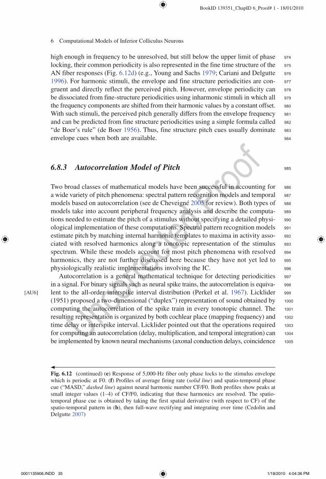
BookID 139351_ChapID 6_Proof# 1 - 18/01/2010
6 Computational Models of Inferior Colliculus Neurons
high enough in frequency to be unresolved, but still below the upper limit of phase locking, their common periodicity is also represented in the fine time structure of the AN fiber responses (Fig. 6.12d) (e.g., Young and Sachs 1979; Cariani and Delgutte 1996). For harmonic stimuli, the envelope and fine structure periodicities are con-gruent and directly reflect the perceived pitch. However, envelope periodicity can be dissociated from fine-structure periodicities using inharmonic stimuli in which all the frequency components are shifted from their harmonic values by a constant offset. With such stimuli, the perceived pitch generally differs from the envelope frequency and can be predicted from fine structure periodicities using a simple formula called “de Boer’s rule” (de Boer 1956). Thus, fine structure pitch cues usually dominate envelope cues when both are available.
6.8.3 Autocorrelation Model of Pitch
Two broad classes of mathematical models have been successful in accounting for a wide variety of pitch phenomena: spectral pattern recognition models and temporal models based on autocorrelation (see de Cheveigné 2005 for review). Both types of models take into account peripheral frequency analysis and describe the computa-tions needed to estimate the pitch of a stimulus without specifying a detailed physi-ological implementation of these computations. Spectral pattern recognition models estimate pitch by matching internal harmonic templates to maxima in activity asso-ciated with resolved harmonics along a tonotopic representation of the stimulus spectrum. While these models account for most pitch phenomena with resolved harmonics, they are not further discussed here because they have not yet led to physiologically realistic implementations involving the IC.
Autocorrelation is a general mathematical technique for detecting periodicities in a signal. For binary signals such as neural spike trains, the autocorrelation is equiva-lent to the all-order interspike interval distribution (Perkel et al. 1967). Licklider (1951) proposed a two-dimensional (“duplex”) representation of sound obtained by computing the autocorrelation of the spike train in every tonotopic channel. The resulting representation is organized by both cochlear place (mapping frequency) and time delay or interspike interval. Licklider pointed out that the operations required for computing an autocorrelation (delay, multiplication, and temporal integration) can be implemented by known neural mechanisms (axonal conduction delays, coincidence
[AU6]
Fig. 6.12 (continued) (e) Response of 5,000-Hz fiber only phase locks to the stimulus envelope which is periodic at F0. (f) Profiles of average firing rate (solid line) and spatio-temporal phase cue (“MASD,” dashed line) against neural harmonic number CF/F0. Both profiles show peaks at small integer values (1–4) of CF/F0, indicating that these harmonics are resolved. The spatio-temporal phase cue is obtained by taking the first spatial derivative (with respect to CF) of the spatio-temporal pattern in (b), then full-wave rectifying and integrating over time (Cedolin and Delgutte 2007)
0001135906.INDD 35 1/18/2010 4:04:36 PM
974
975
976
977
978
979
980
981
982
983
984
985
986
987
988
989
990
991
992
993
994
995
996
997
998
999
1000
1001
1002
1003
1004
1005

BookID 139351_ChapID 6_Proof# 1 - 18/01/2010
K.A. Davis et al.
detection, and lowpass filtering by the membrane capacitance, respectively). Slaney and Lyon (1990) and Meddis and Hewitt (1991) implemented Licklider’s duplex representation using a computational peripheral auditory model as input, and added a stage in which the autocorrelations are summed across all frequency channels to obtain a one-dimensional “summary” or “pooled” autocorrelation. The pitch period is then estimated from the delay of the most prominent maximum (or maxima) in the pooled autocorrelation. The summation across all frequency channels discards all place information and makes the autocorrelation model a purely temporal model invariant to a random shuffling of the tonotopic axis.
The autocorrelation model accounts for the pitches produced by both resolved and unresolved harmonics using the same computations (Meddis and Hewitt 1991). Whereas the autocorrelation model is sensitive to periodicities in both the envelope and the fine structure, the autocorrelation peaks associated with fine structure peri-odicities tend to be sharper than those produced by envelope periodicities, and thus receive more weight in the pooled autocorrelation (Cariani and Delgutte 1996). This is how the autocorrelation model accounts for the pitch shift of inharmonic tones (for which fine structure and envelope periodicities conflict) and for the dominance of low-frequency harmonics that give rise to fine structure cues over high-frequency harmonics that give rise to only envelope cues. However, the autocorrelation model is not sensitive to whether temporal fine structure cues originate from resolved or unresolved harmonics. This conflicts with psychophysical observations showing that resolved harmonics give rise to stronger pitches than unresolved harmonics even when both sets of harmonics occupy the same frequency region (Carlyon and Shackleton 1994; Bernstein and Oxenham 2004). Also, the poor pitch discrimination performance of cochlear implant listeners (Shannon 1983; Carlyon et al. 2002) raises issues for the autocorrelation model because appropriate electrical stimulation creates precise temporal fine structure cues in the auditory nerve (Dynes and Delgutte 1992) that should be detectable by an autocorrelation mechanism. Despite these shortcomings, the autocorrelation model parsimoniously accounts for a large number of psychophysical phenomena and predicts the perceived pitch for a vast majority of the stimuli experienced in everyday listening.
6.8.4 Physiologically Based Models of Pitch Processing
Despite the remarkable effectiveness of the autocorrelation model of pitch, there is no compelling physiological or anatomical evidence for the orderly neural architec-ture of delay lines and coincidence detectors postulated by Licklider (1951). The delays are particularly problematic since detecting the periodicity at the lower limit of pitch near 30 Hz (Pressnitzer et al. 2001) would require an approximately 30 ms delay, which is much longer than the neural latencies typically observed in the brain stem and midbrain. The models presented in this section represent efforts at imple-menting autocorrelation-like processing using neural mechanisms more consistent with the anatomy and physiology of the auditory brain stem.
0001135906.INDD 36 1/18/2010 4:04:36 PM
1006
1007
1008
1009
1010
1011
1012
1013
1014
1015
1016
1017
1018
1019
1020
1021
1022
1023
1024
1025
1026
1027
1028
1029
1030
1031
1032
1033
1034
1035
1036
1037
1038
1039
1040
1041
1042
1043
1044
1045
1046

BookID 139351_ChapID 6_Proof# 1 - 18/01/2010
6 Computational Models of Inferior Colliculus Neurons
The Langner (1981) model circuit discussed in Sect. 6.6.1 is tuned to AM tones with specific modulation and carrier frequencies through coincidence between a delayed trigger signal locked to the modulation frequency and an integrator signal locked to an integer submultiple of the carrier frequency. Thus, a two-dimensional array of such circuits mapped according to both their best carrier frequency and their best modulation frequency provides a periodicity map similar to Licklider’s (1951) duplex representation. This structure is consistent with evidence for roughly orthog-onal maps of best frequency and best modulation frequency in the ICC (Schreiner and Langner 1988). For a SAM tone, the pitch can be estimated from the location of the maximum of activity along the “periodotopy” (modulation frequency) axis of the neural map (Voutsas et al. 2005). For broadband stimuli containing many harmonics, an additional processing stage is required to estimate the pitch from the two-dimensional neural map, either by integrating activity across the tonotopic axis as in the autocor-relation model, or by computing pair wise cross-correlations between all tonotopic channels (Borst et al. 2004).
By requiring coincidence between carrier-locked and modulation-locked signals, the Langner (1981) model can, in principle, account for the pitch of inharmonic stimuli in which the temporal cues in the envelope and the fine structure conflict. Indeed, the periodicity equation describing the dependence of BMF on carrier fre-quency in the Langner model is formally similar5 to the de Boer’s rule for the pitch shift of inharmonic tones (Langner 1985). While this property holds for a neural circuit made up of ideal trigger and integrator neurons receiving inputs that perfectly entrain to the modulation and the carrier, respectively, the robustness of this model for more realistic inputs is an issue, especially in the presence of noise and rever-beration. For example, strong pitches can be evoked by stimuli that have very little amplitude modulation, such as iterated ripple noise or harmonic complex tones in random phase. The model trigger neuron may have trouble reliably firing once per modulation cycle with such stimuli. Also, while the function of the integrator neuron is to count a specific number of carrier cycles before firing, auditory nerve fibers do not fire exactly once per carrier cycle (i.e., they do not entrain). Even if the volley principle is invoked to get a neural signal more directly representing the carrier fre-quency, the robustness of the integrator with intrinsically noisy neural signals as inputs remains an issue. These issues were partly addressed in two implementations of the Langner model that use fairly realistic integrate-and-fire model neurons and receive inputs from a simplified model of the auditory periphery (Borst et al. 2004; Voutsas et al. 2005). So far, both implementations have been tested only with har-monic complex tones having pronounced amplitude modulations. More thorough tests are needed to evaluate the efficacy of this model as a general pitch processor.
5 The periodicity equation gives a linear relationship between best modulation period and carrier period (in which the slope is a ratio of small integers), while de Boers’ rule gives a linear relation-ship between perceived pitch frequency and carrier frequency. The two relationships are very similar when examined over a limited range of carrier frequencies (Langner 1985).
0001135906.INDD 37 1/18/2010 4:04:36 PM
1047
1048
1049
1050
1051
1052
1053
1054
1055
1056
1057
1058
1059
1060
1061
1062
1063
1064
1065
1066
1067
1068
1069
1070
1071
1072
1073
1074
1075
1076
1077
1078
1079
1080
1081
1082
1083
1084

BookID 139351_ChapID 6_Proof# 1 - 18/01/2010
K.A. Davis et al.
The “chopper model of pitch” (Wiegrebe and Meddis 2004), performs an autocorrelation-like operation using physiologically realistic elements based on the Hewitt and Meddis (1994) model for rate tuning to AM frequency in the ICC. In the Hewitt and Meddis (1994) model, rate tuning to AM arises through coincidence between many inputs from VCN chopper neurons that have the same intrinsic chop-ping rate (CR) and best frequency. As in the Licklider (1951) and Langner (1981) models, a two-dimensional temporal representation of sound is first obtained at the VCN stage through a large ensemble of chopper neurons arranged based on both their best frequency and their chopping rate (Fig. 6.13a). This temporal representa-tion of periodicity information is transformed into a two-dimensional rate-based representation at the IC stage through coincidence detection between chopper inputs having the same best frequency and chopping rates. At a final stage of the model (presumably located above the IC), the firing rate of IC neurons is summed across the tonotopic axis for each CR to obtain a one dimensional representation of pitch that plays the same role as the pooled autocorrelation in the Meddis and Hewitt (1991) model (Fig. 6.13a). The model in its present form does not specify how the pitch frequency is estimated from the model output profile. Rather, changes in the shape of the output profile with stimulus manipulations are related to changes in pitch in psychophysical experiments.
Because the model’s effectiveness depends critically on the tuning of chopper neurons to a specific periodicity, the VCN stage of the model has been analyzed in detail (Wiegrebe and Meddis 2004). Model VCN neurons, like real sustained chop-per (Chop-S) neurons, show enhanced representation of the stimulus periodicity in their first-order interspike intervals (i.e., they fire more regularly) when the stimulus F0 matches the neuron’s intrinsic chopping rate (Winter et al. 2001). Importantly, periodicity enhancement in interspike intervals can also occur when the stimulus F0 is a small integer multiple (2 or 4) of the CR. Wiegrebe and Meddis (2004) interpret this result as evidence that chopper neurons act as temporal harmonic templates in the sense that a given chopper neuron would fire highly regularly when a resolved harmonic of a complex tone is an integer multiple of its CR as well as when the fundamental matches its CR. However, the physiological data reported so far only show that a chopper can fire regularly in response to a stimulus whose fundamental (not a resolved harmonic) is a small integer multiple of its CR, which is not quite the same thing since the regular firing to the fundamental could be based on enve-lope cues. Additional physiological data are needed on this important point.
The complete model including the ICC stage (Meddis and O’Mard 2006) shows pitch cues in the activity profile of the output layer as a function of CR but there is no prominent activity peak at the pitch period as in the autocorrelation model (Fig. 6.13b). For stimuli consisting entirely of unresolved harmonics, the profile is basically high-pass (Fig. 6.13b, right), with little activity for low CRs, a steep rise to a shallow maxi-mum when the CR matches the stimulus F0, and then a broad plateau at higher CRs. This plateau arises because chopper neurons with CRs above the F0 fire in synchrony to the stimulus envelope (the F0) rather than to their intrinsic CR. For complex tones with resolved harmonics (Fig. 6.13b, left), the model output pattern shows a steep rise for CRs near the stimulus F0 as in the unresolved case, but then shows a second, shallower
0001135906.INDD 38 1/18/2010 4:04:36 PM
1085
1086
1087
1088
1089
1090
1091
1092
1093
1094
1095
1096
1097
1098
1099
1100
1101
1102
1103
1104
1105
1106
1107
1108
1109
1110
1111
1112
1113
1114
1115
1116
1117
1118
1119
1120
1121
1122
1123
1124
1125
1126
1127
1128
1129
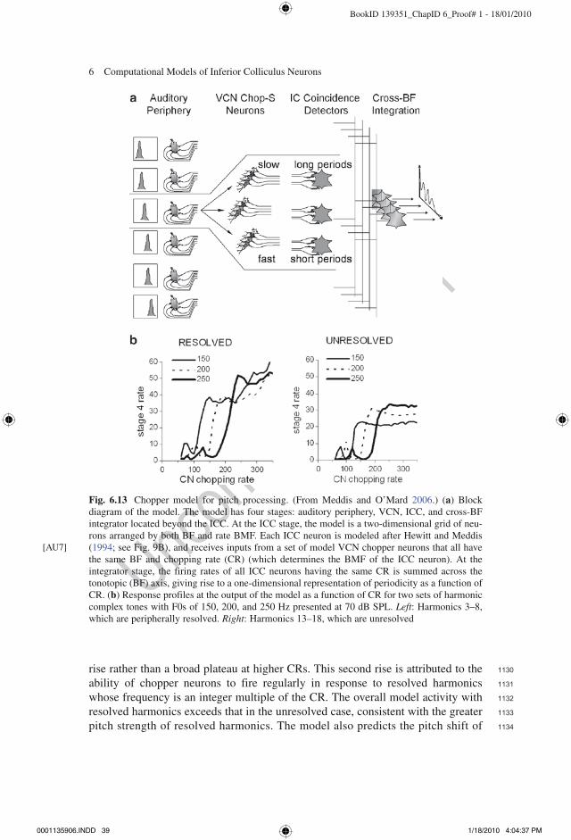
BookID 139351_ChapID 6_Proof# 1 - 18/01/2010
6 Computational Models of Inferior Colliculus Neurons
Fig. 6.13 Chopper model for pitch processing. (From Meddis and O’Mard 2006.) (a) Block diagram of the model. The model has four stages: auditory periphery, VCN, ICC, and cross-BF integrator located beyond the ICC. At the ICC stage, the model is a two-dimensional grid of neu-rons arranged by both BF and rate BMF. Each ICC neuron is modeled after Hewitt and Meddis (1994; see Fig. 9B), and receives inputs from a set of model VCN chopper neurons that all have the same BF and chopping rate (CR) (which determines the BMF of the ICC neuron). At the integrator stage, the firing rates of all ICC neurons having the same CR is summed across the tonotopic (BF) axis, giving rise to a one-dimensional representation of periodicity as a function of CR. (b) Response profiles at the output of the model as a function of CR for two sets of harmonic complex tones with F0s of 150, 200, and 250 Hz presented at 70 dB SPL. Left: Harmonics 3–8, which are peripherally resolved. Right: Harmonics 13–18, which are unresolved
[AU7]
rise rather than a broad plateau at higher CRs. This second rise is attributed to the ability of chopper neurons to fire regularly in response to resolved harmonics whose frequency is an integer multiple of the CR. The overall model activity with resolved harmonics exceeds that in the unresolved case, consistent with the greater pitch strength of resolved harmonics. The model also predicts the pitch shift of
0001135906.INDD 39 1/18/2010 4:04:37 PM
1130
1131
1132
1133
1134

BookID 139351_ChapID 6_Proof# 1 - 18/01/2010
K.A. Davis et al.
inharmonic tones when the harmonics are resolved but not when they are unresolved, broadly consistent with psychophysical data (Moore and Moore 2003).
The chopper model of pitch represents the most comprehensive and thoroughly tested effort at developing a physiologically realistic model for pitch processing to date. There are nevertheless a number of issues with this model. First, the model has mostly been tested with a narrow range of F0s near 200 Hz. With such stimuli, resolved harmonics are typically within the frequency range (<1,000–1,500 Hz) where VCN choppers phase lock to the fine structure (Blackburn and Sachs 1989), while unresolved harmonics are always above the upper limit of phase locking. Thus, the differences in model behavior attributed to differences in harmonic resolv-ability may actually reflect differences between pitch cues available in the temporal fine structure vs. the envelope of the responses of chopper neurons. Harmonics located in the 1,800- to 3,000-Hz region (above the upper limit of phase locking in choppers) can give rise to strong pitch sensations in human listeners, and also show sharp perceptual differences between resolved and unresolved harmonics (Carlyon and Shackleton 1994; Bernstein and Oxenham 2004). It will be important to test this condition with the model by varying F0 over a wider range. A second issue is that the model output profile for harmonic complex tones is sensitive not only to changes in F0 that affect the pitch, but also to changes in harmonic composition (timbre) and stimulus level that produce no change in pitch. The present strategy of looking at changes in model output profiles associated with changes in pitch may not work for psychophysical experiments where stimulus level and harmonic composition are randomized. To account for performance in such experiments, it may be necessary to identify a specific feature associated with pitch in the model output profile. Because small changes in F0 can produce widespread changes in the model output that are not restricted to CRs near the F0 (Fig. 5a in Meddis and O’Mard 2006), identifying a such a feature may prove challenging. A third and more fundamental issue with the model is that the 100- to 500-Hz range of intrinsic CRs typically observed in VCN neurons (Frisina et al. 1990) covers only a portion of the 30- to 1,400-Hz range of F0 that produce pitch percepts with missing fundamental stimuli in human listeners As mentioned in the preceding text, if the coincidence detector is located in ICC (as assumed by the model), there is a further mismatch between the range of VCN chopping rates and the 10- to 150-Hz range where most IC neurons have their best modulation frequencies (Krishna and Semple 2000).
6.9 Summary
We have reviewed a wide variety of models that aim at accounting for emerging response properties of IC neurons in terms of interactions between various inputs to the IC and circuitry within the IC itself. These models assume specific neural cir-cuits to model specific aspects of spatial hearing or temporal processing. While these models have advanced our understanding of how response properties may be formed, they leave us yet far from a comprehensive understanding of IC function.
0001135906.INDD 40 1/18/2010 4:04:37 PM
1135
1136
1137
1138
1139
1140
1141
1142
1143
1144
1145
1146
1147
1148
1149
1150
1151
1152
1153
1154
1155
1156
1157
1158
1159
1160
1161
1162
1163
1164
1165
1166
1167
1168
1169
1170
1171
1172
1173
1174
1175

BookID 139351_ChapID 6_Proof# 1 - 18/01/2010
6 Computational Models of Inferior Colliculus Neurons
Such a comprehensive view might be furthered by a focus on the integration of stimulus features, and a clearer identification of essential commonalities across models.
Despite the wide range of modeling strategies and phenomena being modeled, the models use a small number of basic circuit modules much like bricks in a Lego game. Prominent among these is coincidence detection which sharpens temporal response patterns and can also transform a temporal code into a rate or rate-place code. Coincidence detection, first proposed by Jeffress (1948), is used in models for ITD processing in the MSO (Colburn, Chap. 4), in models for generating Onset response patterns in the cochlear nucleus (Voigt, Chap. 3), and in models for rate tuning to modulation frequency and periodicity detection in the IC (Langner 1981; Hewitt and Meddis 1994; Meddis and O’Mard 2006). Contrasting with coincidence detection, which is a highly nonlinear interaction between excitatory inputs, is the additive sum-mation of excitatory inputs used in the Shackleton et al. (2000) model. Also widely used is the interplay between excitatory and inhibitory inputs which can perform a wide variety of signal processing operations depending on the characteristics of the inhibition. Inhibition can be either temporally precise (phase locked) as in models for ITD sensitivity in MSO (Brand et al. 2002) and AM tuning in MSO and IC (Grothe 1994; Nelson and Carney 2004), or be delayed and persistent to create a long-term dependence on previous inputs (Cai et al. 1998a; Pecka et al. 2007). Inhibition can also be lateral to sharpen tuning to a stimulus feature along a neural map (Cai et al. 1998a; Rucci and Wray 1999; Kimball et al. 2003; Dicke et al. 2007).
Whereas interactions between synaptic inputs have been the main workhorse of computational IC models, the role of intrinsic membrane channels, which play an important role in models of cochlear nucleus neurons (Voigt, Chap. 3), has been relatively unexplored. Only two models (Cai et al. 1998b; Borisyuk et al. 2002) explicitly introduced membrane conductances for dynamic processing, and there has been no effort to exploit the signal processing capabilities of the arsenal of membrane channels documented in IC neurons (Sivaramakrishnan and Oliver 2001; Wu et al. 2002). This omission is particularly surprising for models of AM tuning, where it would seem to be natural. Another omission is that all IC models use a strictly feed-forward architecture and thus do not take advantage of the signal processing capabilities of recurrent connections (Cariani 2001; Friedel et al. 2007). Recurrent connections are widespread in the central nervous system, and the exis-tence of intricate circuitry within the IC, commissural connections between the two ICs (Saldaña and Merchán 2005) and descending projections from the thalamus and cortex (Winer 2005) suggest that feedback may play an important role in IC pro-cessing (Suga and Ma 2003).
Perhaps the main limitation of IC models so far has been their focus on a rather narrow set of physiological phenomena. Binaural IC models focus on either ITD or ILD processing, and consider only inputs from MSO and LSO, respectively, while temporal processing models focus on the transformation from a temporal code to a rate code for AM tuning, and consider only direct, monaural inputs from the CN. In reality, the vast majority of IC neurons are sensitive to both binaural cues and amplitude modulation, and physiological studies reveal interactions between binaural and temporal processing (Sterbing et al. 2003; Lane and Delgutte 2005).
[AU8]
0001135906.INDD 41 1/18/2010 4:04:37 PM
1176
1177
1178
1179
1180
1181
1182
1183
1184
1185
1186
1187
1188
1189
1190
1191
1192
1193
1194
1195
1196
1197
1198
1199
1200
1201
1202
1203
1204
1205
1206
1207
1208
1209
1210
1211
1212
1213
1214
1215
1216
1217
1218
1219
1220
BookID 139351_ChapID 6_Proof# 1 - 18/01/2010
K.A. Davis et al.
Also, a majority of IC neurons are sensitive to both ITD and ILD (Chase and Young 2005), particularly when tested with broadband stimuli. An important next step will be to integrate models of binaural, temporal, and spectral processing to develop a more comprehensive view of IC function. A major stumbling block toward this goal is the lack of physiological criteria for identifying the types of brain stem inputs that a given IC neuron receives. Such criteria are well established for the cochlear nucleus where there is a clear correspondence between anatomical cell types and physiological types defined from tone-burst response patterns and frequency response maps, but this type of understanding has been slow to emerge for the IC. Recent progress in this important area is encouraging (Ramachandran et al. 1999; Davis 2002; Loftus et al. 2004; Malmierca et al. 2005). Another stumbling block is that physiological studies typically report only a fairly narrow set of response prop-erties from each neuron, even when the neuron was actually tested with a wide range of stimulus conditions. Perhaps the increased availability of publicly accessible databases of physiological data can remedy this problem.
Despite the limitations of present IC models, the very fact that this topic could be reviewed indicates the enormous progress that has been made since the first edition of this book in 1996. We may be at the threshold of developing a more integrative understanding of IC function in which computational modeling will undoubtedly play a key role.
Acknowledgment We thank M. Slama, G.I. Wang, L. Wang, B. Wen, and Y Zhou for their com-ments on the manuscript, and G.I. Wang for help with figure preparation. Preparation of this chapter was supported by NIH grants DC002258 (Delgutte and Hancock) and DC05161 (Davis).
References
Aitkin LM (1986) The Auditory Midbrain: Structure and Function of the Central Auditory Pathway. Clifton, NJ: Humana.
Batra R, Kuwada S, Fitzpatrick DC (1997a) Sensitivity to interaural temporal disparities of low- and high-frequency neurons in the superior olivary complex. I. Heterogeneity of responses. J Neurophysiol 78:1222–1236.
Batra R, Kuwada S, Fitzpatrick DC (1997b) Sensitivity to interaural temporal disparities of low- and high-frequency neurons in the superior olivary complex. II. Coincidence detection. J Neurophysiol 78:1237–1247.
Bernstein JG, Oxenham AJ (2003) Pitch discrimination of diotic and dichotic tone complexes: harmonic resolvability or harmonic number? J Acoust Soc Am 113:3323–3334.
Bernstein JG, Oxenham AJ (2004) Effect of stimulus level and harmonic resolvability on pitch discrimination. J Acoust Soc Am 115:2389.
Blackburn CC, Sachs MB (1989) Classification of unit types in the anteroventral cochlear nucleus: PST histograms and regularity analysis. J Neurophysiol 62:1303–1329.
Borisyuk A, Semple MN, Rinzel J (2001) Computational model for the dynamic aspects of sound processing in the auditory midbrain. Neurocomputing 38–40:1127–1134.
Borisyuk A, Semple MN, Rinzel J (2002) Adaptation and inhibition underlie responses to time-varying interaural phase cues in a model of inferior colliculus neurons. J Neurophysiol 88: 2134–2146.
0001135906.INDD 42 1/18/2010 4:04:37 PM
1221
1222
1223
1224
1225
1226
1227
1228
1229
1230
1231
1232
1233
1234
1235
1236
1237
1238
1239
1240
1241
1242
1243
1244
1245
1246
1247
1248
1249
1250
1251
1252
1253
1254
1255
1256
1257
1258
1259
1260
1261
1262
1263

BookID 139351_ChapID 6_Proof# 1 - 18/01/2010
6 Computational Models of Inferior Colliculus Neurons
Borst M, Langner G, Palm G (2004) A biologically motivated neural network for phase extraction from complex sounds. Biol Cybern 90:98–104.
Boudreau JC, Tsuchitani C (1968) Binaural interaction in the cat superior olive S segment. J Neurophysiol 31:442–454.
Braasch J, Blauert J (2003) The precedence effect for noise bursts of different bandwidths. II. Comparison of model algorithms. Acoust Sci Technol 24:293–303.
Brand A, Behrend O, Marquardt T, McAlpine D, Grothe B (2002) Precise inhibition is essential for microsecond interaural time difference coding. Nature 417:543–547.
Brughera A, Stutman E, Carney LH, Colburn HS (1996) A model for excitation and inhibition for cells in the medial superior olive. Audit Neurosci 2:219–233.
Burger RM, Pollak GD (2001) Reversible inactivation of the dorsal nucleus of the lateral lemnis-cus reveals its role in the processing of multiple sound sources in the inferior colliculus of bats. J Neurosci 21:4830–4843.
Cai H, Carney LH, Colburn HS (1998a) A model for binaural response properties of inferior colliculus neurons. I. A model with interaural time difference-sensitive excitatory and inhibi-tory inputs. J Acoust Soc Am 103:475–493.
Cai H, Carney LH, Colburn HS (1998b) A model for binaural response properties of inferior colliculus neurons. II. A model with interaural time difference-sensitive excitatory and inhibitory inputs and an adaptation mechanism. J Acoust Soc Am 103:494–506.
Caird D, Klinke R (1983) Processing of binaural stimuli by cat superior olivary complex neurons. Exp Brain Res 52:385–399.
Cant NB (2005) Projections from the cochlear nuclear complex to the inferior colliculus. In: Winer JA, Schreiner CE (eds), The Inferior Colliculus. New York: Springer, pp 115–131.
Cariani PA (2001) Neural timing nets. Neural Netw 14:737–753.Cariani PA, Delgutte B (1996) Neural correlates of the pitch of complex tones. I. Pitch and pitch
salience. J Neurophysiol 76:1698–1716.Carlyon RP, Shackleton TM (1994) Comparing the fundamental frequencies of resolved and
unresolved harmonics: evidence for two pitch mechanisms? J Acoust Soc Am 95:3541–3554.
Carlyon RP, van Wieringen A, Long CJ, Deeks JM, Wouters J (2002) Temporal pitch mechanisms in acoustic and electric hearing. J Acoust Soc Am 112:621–633.
Carney LH (1993) A model for the responses of low-frequency auditory-nerve fibers in cat. J Acoust Soc Am 93:401–417.
Casseday JH, Covey E (1996) A neuroethological theory of the operation of the inferior colliculus. Brain Behav Evol 47:311–336.
Cedolin L, Delgutte B (2005) Pitch of complex tones: rate-place and interspike interval represen-tations in the auditory nerve. J Neurophysiol 94:347–362.
Cedolin L, Delgutte B (2007) Spatio-temporal representation of the pitch of complex tones in the auditory nerve. In: Kollmeier B, Klump G, Hohmann V, Langemann U, Mauermann M, Uppenkamp S, Verhey J (eds), Hearing – From Sensory Processing to Perception Heidelberg: Springer, pp 61–70.
Chase SM, Young ED (2005) Limited segregation of different types of sound localization informa-tion among classes of units in the inferior colliculus. J Neurosci 25:7575–7585.
Colburn HS (1996) Computational models of binaural processing. In: Hawkins HH, McMullen TA, Popper AN, Fay RR (eds), Auditory Computation. New York: Springer, pp 332–401.
Darwin CJ, Carlyon RP (1995) Auditory grouping. In: Moore BCJ (ed), The Handbook of Perception and Cognition. New York: Academic, pp 387–424.
Davis KA (2002) Evidence of a functionally segregated pathway from dorsal cochlear nucleus to inferior colliculus. J Neurophysiol 87:1824–1835.
Davis KA, Ramachandran R, May BJ (1999) Single-unit responses in the inferior colliculus of decerebrate cats. II. Sensitivity to interaural level differences. J Neurophysiol 82:164–175.
Davis KA, Ramachandran R, May BJ (2003) Auditory processing of spectral cues for sound localization in the inferior colliculus. J Assoc Res Otolaryngol 4:148–163.
de Boer E (1956) On the “Residue” in Hearing. In: University of Amsterdam.[AU9]
0001135906.INDD 43 1/18/2010 4:04:38 PM
1264
1265
1266
1267
1268
1269
1270
1271
1272
1273
1274
1275
1276
1277
1278
1279
1280
1281
1282
1283
1284
1285
1286
1287
1288
1289
1290
1291
1292
1293
1294
1295
1296
1297
1298
1299
1300
1301
1302
1303
1304
1305
1306
1307
1308
1309
1310
1311
1312
1313
1314
1315
1316
1317

BookID 139351_ChapID 6_Proof# 1 - 18/01/2010
K.A. Davis et al.
de Cheveigné A (2005) Pitch perception models. In: Plack CJ, Oxenham AJ, Fay RR, Popper AN (eds), Pitch Neural Coding and Perception. New York: Springer, pp 169–233.
Devore S, Ihlefeld A, Hancock K, Shinn-Cunningham B, Delgutte B (2009) Accurate sound localization in reverberant environments is mediated by robust encoding of spatial cues in the auditory midbrain. Neuron 62:123–134.
Dicke U, Ewert SD, Dau T, Kollmeier B (2007) A neural circuit transforming temporal periodicity information into a rate-based representation in the mammalian auditory system. J Acoust Soc Am 121:310–326.
Dong CJ, Swindale NV, Zakarauskas P, Hayward V, Cynader MS (2000) The auditory motion aftereffect: its tuning and specificity in the spatial and frequency domains. Percept Psychophys 62:1099–1111.
Dynes SB, Delgutte B (1992) Phase-locking of auditory-nerve discharges to sinusoidal electric stimulation of the cochlea. Hear Res 58:79–90.
Ehret G, Romand R, eds (1997) The Central Auditory System. New York: Oxford University Press.Fitzpatrick DC, Kuwada S, Kim DO, Parham K, Batra R (1999) Responses of neurons to click-
pairs as simulated echoes: auditory nerve to auditory cortex. J Acoust Soc Am 106:3460–3472.Friedel P, Burck M, Leo van Hemmen J (2007) Neuronal identification of acoustic signal periodic-
ity. Biol Cybern 97:247–260.Frisina RD, Smith RL, Chamberlain SC (1990) Encoding of amplitude modulation in the gerbil
cochlear nucleus: I. A hierarchy of enhancement. Hear Res 44:99–122.Geis HR, Borst JG (2009) Intracellular responses of neurons in the mouse inferior colliculus to
sinusoidal amplitude-modulated tones. J Neurophysiol 101:2002–2016.Goldberg JM, Brown PB (1969) Response of binaural neurons of dog superior olivary complex to
dichotic tonal stimuli: some physiological mechanisms of sound localization. J Neurophysiol 32:613–636.
Grantham DW (1998) Auditory motion aftereffects in the horizontal plane: the effects of spectral region, spatial sector, and spatial richness. Acustica 84:337–347.
Grantham DW, Wightman FL (1978) Detectability of varying interaural temporal differences. J Acoust Soc Am 63:511–523.
Green DM, Swets JA (1988) Signal Detection Theory and Psychophysics. Los Altos, CA: Peninsula.
Griffiths TD, Rees G, Rees A, Green GG, Witton C, Rowe D, Buchel C, Turner R, Frackowiak RS (1998) Right parietal cortex is involved in the perception of sound movement in humans. Nat Neurosci 1:74–79.
Grothe B, Covey E, Casseday JH (2001) Medial superior olive of the big brown bat: neuronal responses to pure tones, amplitude modulations, and pulse trains. J Neurophysiol 86: 2219–2230.
Guerin A, Jeannes Rle B, Bes J, Faucon G, Lorenzi C (2006) Evaluation of two computational models of amplitude modulation coding in the inferior colliculus. Hear Res 211:54–62.
Hancock KE (2007) A physiologically-based population rate code for interaural time differences (ITDs) predicts bandwidth-dependent lateralization. In: Kollmeier B, Klump G, Hohmann V, Langemann U, Mauermann M, Uppenkamp S, Verhey J (eds), Hearing – From Sensory Processing to Perception. Heidelberg: Springer, pp 389–397.
Hancock KE, Delgutte B (2004) A physiologically based model of interaural time difference discrimination. J Neurosci 24:7110–7117.
Hancock KE, Voigt HF (1999) Wideband inhibition of dorsal cochlear nucleus type IV units in cat: a computational model. Ann Biomed Eng 27:73–87.
Harper NS, McAlpine D (2004) Optimal neural population coding of an auditory spatial cue. Nature 430:682–686.
Hartung K, Trahiotis C (2001) Peripheral auditory processing and investigations of the “prece-dence effect” which utilize successive transient stimuli. J Acoust Soc Am 110:1505–1513.
Hewitt MJ, Meddis R (1994) A computer model of amplitude-modulation sensitivity of single units in the inferior colliculus. J Acoust Soc Am 95:2145–2159.
0001135906.INDD 44 1/18/2010 4:04:38 PM
1318
1319
1320
1321
1322
1323
1324
1325
1326
1327
1328
1329
1330
1331
1332
1333
1334
1335
1336
1337
1338
1339
1340
1341
1342
1343
1344
1345
1346
1347
1348
1349
1350
1351
1352
1353
1354
1355
1356
1357
1358
1359
1360
1361
1362
1363
1364
1365
1366
1367
1368
1369
1370
BookID 139351_ChapID 6_Proof# 1 - 18/01/2010
6 Computational Models of Inferior Colliculus Neurons
Hewitt MJ, Meddis R, Shackleton TM (1992) A computer model of a cochlear-nucleus stellate cell: responses to amplitude-modulated and pure-tone stimuli. J Acoust Soc Am 91:2096–2109.
Jeffress LA (1948) A place theory of sound localization. J Comp Physiol Psychol 41:35–39.Joris PX, Yin TC (1998) Envelope coding in the lateral superior olive. III. Comparison with afferent
pathways. J Neurophysiol 79:253–269.Joris PX, Schreiner CE, Rees A (2004) Neural processing of amplitude-modulated sounds.
Physiol Rev 84:541–577.Keller CH, Takahashi TT (1996) Binaural cross-correlation predicts the responses of neurons in
the owl’s auditory space map under conditions simulating summing localization. J Neurosci 16:4300–4309.
Kimball J, Lomakin O, Davis KA (2003) A computational model of spectral processing pathway from dorsal cochlear nucleus to inferior colliculus. In: BME Annual Fall Meeting, Nashville, TN, p 173.
Krishna BS, Semple MN (2000) Auditory temporal processing: responses to sinusoidally amplitude-modulated tones in the inferior colliculus. J Neurophysiol 84:255–273.
Lane CC, Delgutte B (2005) Neural correlates and mechanisms of spatial release from masking: single-unit and population responses in the inferior colliculus. J Neurophysiol 94:1180–1198.
Langner G (1981) Neuronal mechanisms for pitch analysis in the time domain. Exp Brain Res 44:450–454.
Langner G (1983) Evidence for neuronal periodicity detection in the auditory system of the Guinea fowl: implications for pitch analysis in the time domain. Exp Brain Res 52:333–355.
Langner G (1985) Time coding and periodicity pitch. In: Michelsen A (ed), Time Resolution in Auditory Systems. Heidelberg: Springer, pp 108–121.
Langner G (1992) Periodicity coding in the auditory system. Hear Res 60:115–142.Langner G, Schreiner CE (1988) Periodicity coding in the inferior colliculus of the cat. I. Neuronal
mechanisms. J Neurophysiol 60:1799–1822.Langner G, Albert M, Briede T (2002) Temporal and spatial coding of periodicity information in
the inferior colliculus of awake chinchilla (Chinchilla laniger). Hear Res 168:110–130.Li L, Kelly JB (1992) Inhibitory influence of the dorsal nucleus of the lateral lemniscus on binau-
ral responses in the rat’s inferior colliculus. J Neurosci 12:4530–4539.Lindemann W (1986) Extension of a binaural cross-correlation model by contralateral inhibition.
II. The law of the first wave front. J Acoust Soc Am 80:1623–1630.Litovsky RY, Yin TC (1998) Physiological studies of the precedence effect in the inferior colliculus
of the cat. II. Neural mechanisms. J Neurophysiol 80:1302–1316.Litovsky RY, Colburn HS, Yost WA, Guzman SJ (1999) The precedence effect. J Acoust Soc Am
106:1633–1654.Liu LF, Palmer AR, Wallace MN (2006) Phase-locked responses to pure tones in the inferior col-
liculus. J Neurophysiol 95:1926–1935.Loftus WC, Bishop DC, Saint Marie RL, Oliver DL (2004) Organization of binaural excitatory and
inhibitory inputs to the inferior colliculus from the superior olive. J Comp Neurol 472:330–344.Malmierca MS, Saint Marie RL, Merchán MA, Oliver DL (2005) Laminar inputs from dorsal
cochlear nucleus and ventral cochlear nucleus to the central nucleus of the inferior colliculus: two patterns of convergence. Neuroscience 136:883–894.
McAlpine D, Palmer AR (2002) Blocking GABAergic inhibition increases sensitivity to sound motion cues in the inferior colliculus. J Neurosci 22:1443–1453.
McAlpine D, Jiang D, Shackleton TM, Palmer AR (1998) Convergent input from brainstem coincidence detectors onto delay-sensitive neurons in the inferior colliculus. J Neurosci 18:6026–6039.
McAlpine D, Jiang D, Shackleton TM, Palmer AR (2000) Responses of neurons in the inferior colliculus to dynamic interaural phase cues: evidence for a mechanism of binaural adaptation. J Neurophysiol 83:1356–1365.
McAlpine D, Jiang D, Palmer AR (2001) A neural code for low-frequency sound localization in mammals. Nat Neurosci 4:396–401.
0001135906.INDD 45 1/18/2010 4:04:38 PM
1371
1372
1373
1374
1375
1376
1377
1378
1379
1380
1381
1382
1383
1384
1385
1386
1387
1388
1389
1390
1391
1392
1393
1394
1395
1396
1397
1398
1399
1400
1401
1402
1403
1404
1405
1406
1407
1408
1409
1410
1411
1412
1413
1414
1415
1416
1417
1418
1419
1420
1421
1422
1423

BookID 139351_ChapID 6_Proof# 1 - 18/01/2010
K.A. Davis et al.
Meddis R, Hewitt MJ (1991) Virtual pitch and phase sensitivity of a computer model of the auditory periphery. I. Pitch identification. J Acoust Soc Am 89:2866–2882.
Meddis R, O’Mard L (2006) Virtual pitch in a computational physiological model. J Acoust Soc Am 120:3861–3869.
Middlebrooks JC, Green DM (1991) Sound localization by human listeners. Annu Rev Psychol 42:135–159.
Moore GA, Moore BC (2003) Perception of the low pitch of frequency-shifted complexes. J Acoust Soc Am 113:977–985.
Mossop JE, Culling JF (1998) Lateralization of large interaural delays. J Acoust Soc Am 104:1574–1579.
Nelson PC, Carney LH (2004) A phenomenological model of peripheral and central neural responses to amplitude-modulated tones. J Acoust Soc Am 116:2173–2186.
Nelson PC, Carney LH (2007) Neural rate and timing cues for detection and discrimination of amplitude-modulated tones in the awake rabbit inferior colliculus. J Neurophysiol 97:522–539.
Oliver DL (2005) Neuronal organization in the inferior colliculus. In: Winer JA, Schreiner CE (eds), The Inferior Colliculus. New York: Springer, pp 69–114.
Oliver DL, Huerta MF (1992) Inferior and superior colliculi. In: Webster DB, Popper AN, Fay RR (eds), The Mammalian Auditory Pathway: Neuroanatomy. New York: Springer, pp 168–222.
Oliver DL, Morest DK (1984) The central nucleus of the inferior colliculus in the cat. J Comp Neurol 222:237–264.
Oliver DL, Beckius GE, Bishop DC, Kuwada S (1997) Simultaneous anterograde labeling of axonal layers from lateral superior olive and dorsal cochlear nucleus in the inferior colliculus of cat. J Comp Neurol 382:215–229.
Palmer AR, Kuwada S (2005) Binaural and spatial coding in the inferior colliculus. In: Winer JA, Schreiner CE (eds), The Inferior Colliculus. New York: Springer, pp 377–410.
Park TJ, Pollak GD (1993) GABA shapes sensitivity to interaural intensity disparities in the mustache bat’s inferior colliculus: implications for encoding sound location. J Neurosci 13:2050–2067.
Paterson M, McAlpine D (2005) Effects of peripheral processing are evident in neural correlates of precedence effect. Assoc Res Otolaryn Abstr 28:1414.
Pecka M, Zahn TP, Saunier-Rebori B, Siveke I, Felmy F, Wiegrebe L, Klug A, Pollak GD, Grothe B (2007) Inhibiting the inhibition: a neuronal network for sound localization in reverberant envi-ronments. J Neurosci 27:1782–1790.
Peña JL, Konishi M (2001) Auditory spatial receptive fields created by multiplication. Science 292:249–252.
Perkel D, Gerstein G, Moore G (1967) Neuronal spike trains and stochastic point processes: I. The single spike train. Biophys J 7:391–418.
Plack CJ, Oxenham AJ (2005) The psychophysics of pitch. In: Plack CJ, Oxenham AJ, Fay RR, Popper AN (eds), Pitch Neural Coding and Perception. New York: Springer, pp 7–55.
Plomp R (1964) The ear as a frequency analyzer. J Acoust Soc Am 36:1628–1636.Pollak GD, Burger RM, Park TJ, Klug A, Bauer EE (2002) Roles of inhibition for transforming
binaural properties in the brainstem auditory system. Hear Res 168:60–78.Pressnitzer D, Patterson RD, Krumbholz K (2001) The lower limit of melodic pitch. J Acoust Soc
Am 109:2074–2084.Ramachandran R, Davis KA, May BJ (1999) Single-unit responses in the inferior colliculus of
decerebrate cats. I. Classification based on frequency response maps. J Neurophysiol 82:152–163.
Reed MC, Blum JJ (1999) Model calculations of steady state responses to binaural stimuli in the dorsal nucleus of the lateral lemniscus. Hear Res 136:13–28.
Rees A, Langner G (2005) Temporal coding in the auditory midbrain. In: Winer JA, Schreiner CE (eds), The Inferior Colliculus. New York: Springer, pp 346–376.
Rhode WS, Greenberg S (1994) Encoding of amplitude modulation in the cochlear nucleus of the cat. J Neurophysiol 71:1797–1825.
Rosen S (1992) Temporal information in speech: acoustic, auditory and linguistic aspects. Philos Trans R Soc Lond B Biol Sci 336:367–373.
0001135906.INDD 46 1/18/2010 4:04:38 PM
1424
1425
1426
1427
1428
1429
1430
1431
1432
1433
1434
1435
1436
1437
1438
1439
1440
1441
1442
1443
1444
1445
1446
1447
1448
1449
1450
1451
1452
1453
1454
1455
1456
1457
1458
1459
1460
1461
1462
1463
1464
1465
1466
1467
1468
1469
1470
1471
1472
1473
1474
1475
1476
1477

BookID 139351_ChapID 6_Proof# 1 - 18/01/2010
6 Computational Models of Inferior Colliculus Neurons
Rothman JS, Young ED, Manis PB (1993) Convergence of auditory nerve fibers onto bushy cells in the ventral cochlear nucleus: implications of a computational model. J Neurophysiol 70:2562–2583.
Rucci M, Wray J (1999) Binaural cross-correlation and auditory localization in the barn owl: a theoretical study. Neural Netw 12:31–42.
Sachs MB, Young ED (1979) Encoding of steady-state vowels in the auditory nerve: representa-tion in terms of discharge rate. J Acoust Soc Am 66:470–479.
Saldaña E, Merchán MA (2005) Intrinsic and commissural connections of the inferior colliculus. In: Winer JA, Schreiner CE (eds), The Inferior Colliculus. New York: Springer, pp 155–181.
Sanes DH, Malone BJ, Semple MN (1998) Role of synaptic inhibition in processing of dynamic binaural level stimuli. J Neurosci 18:794–803.
Schofield BR (2005) Superior olivary complex and lateral lemniscal connections of the auditory midbrain. In: Winer JA, Schreiner CE (eds), The Inferior Colliculus. New York: Springer, pp 132–154.
Schreiner CE, Langner G (1988) Periodicity coding in the inferior colliculus of the cat. II. Topographical organization. J Neurophysiol 60:1823–1840.
Shackleton TM, Meddis R, Hewitt MJ (1992) Across frequency integration in a model of lateral-ization. J Acoust Soc Am 91:2276–2279.
Shackleton TM, McAlpine D, Palmer AR (2000) Modelling convergent input onto interaural-delay-sensitive inferior colliculus neurones. Hear Res 149:199–215.
Shamma SA (1985) Speech processing in the auditory system. I: The representation of speech sounds in the responses of the auditory nerve. J Acoust Soc Am 78:1612–1621.
Shannon RV (1983) Multichannel electrical stimulation of the auditory nerve in man. I. Basic psychophysics. Hear Res 11:157–189.
Singh NC, Theunissen FE (2003) Modulation spectra of natural sounds and ethological theories of auditory processing. J Acoust Soc Am 114:3394–3411.
Sivaramakrishnan S, Oliver DL (2001) Distinct K currents result in physiologically distinct cell types in the inferior colliculus of the rat. J Neurosci 21:2861–2877.
Slaney M, Lyon RF (1990) A perceptual pitch detector. Proc IEEE-ICASSP-90:357–360.Spitzer MW, Semple MN (1993) Responses of inferior colliculus neurons to time-varying inter-
aural phase disparity: effects of shifting the locus of virtual motion. J Neurophysiol 69:1245–1263.
Spitzer MW, Semple MN (1998) Transformation of binaural response properties in the ascending auditory pathway: influence of time-varying interaural phase disparity. J Neurophysiol 80:3062–3076.
Srulovicz P, Goldstein JL (1983) A central spectrum model: a synthesis of auditory-nerve timing and place cues in monaural communication of frequency spectrum. J Acoust Soc Am 73:1266–1276.
Steeneken HJ, Houtgast T (1980) A physical method for measuring speech-transmission quality. J Acoust Soc Am 67:318–326.
Sterbing SJ, D’Angelo WR, Ostapoff EM, Kuwada S (2003) Effects of amplitude modulation on the coding of interaural time differences of low-frequency sounds in the inferior colliculus. I. Response properties. J Neurophysiol 90:2818–2826.
Stern RM, Zeiberg AS, Trahiotis C (1988) Lateralization of complex binaural stimuli: a weighted-image model. J Acoust Soc Am 84:156–165.
Suga N, Ma X (2003) Multiparametric corticofugal modulation and plasticity in the auditory system. Nat Rev 4:783–794.
Tollin DJ, Yin TC (2002a) The coding of spatial location by single units in the lateral superior olive of the cat. I. Spatial receptive fields in azimuth. J Neurosci 22:1454–1467.
Tollin DJ, Yin TC (2002b) The coding of spatial location by single units in the lateral superior olive of the cat. II. The determinants of spatial receptive fields in azimuth. J Neurosci 22:1468–1479.
Voutsas K, Langner G, Adamy J, Ochse M (2005) A brain-like neural network for periodicity analysis. IEEE Trans Syst Man Cybern B Cybern 35:12–22.
0001135906.INDD 47 1/18/2010 4:04:38 PM
1478
1479
1480
1481
1482
1483
1484
1485
1486
1487
1488
1489
1490
1491
1492
1493
1494
1495
1496
1497
1498
1499
1500
1501
1502
1503
1504
1505
1506
1507
1508
1509
1510
1511
1512
1513
1514
1515
1516
1517
1518
1519
1520
1521
1522
1523
1524
1525
1526
1527
1528
1529
1530
1531
BookID 139351_ChapID 6_Proof# 1 - 18/01/2010
K.A. Davis et al.
Wiegrebe L, Meddis R (2004) The representation of periodic sounds in simulated sustained chopper units of the ventral cochlear nucleus. J Acoust Soc Am 115:1207–1218.
Winer JA (2005) Three systems of descending projections to the inferior colliculus. In: Winer JA, Schreiner CE (eds), The Inferior Colliculus. New York: Springer, pp 231–247.
Winer JA, Schreiner CE, eds (2005) The Inferior Colliculus. New York: Springer.Winter IM, Wiegrebe L, Patterson RD (2001) The temporal representation of the delay of iterated
rippled noise in the ventral cochlear nucleus of the guinea-pig. J Physiol 537:553–566.Wu SH, Ma CL, Sivaramakrishnan S, Oliver DL (2002) Synaptic modification in neurons of the
central nucleus of the inferior colliculus. Hear Res 168:43–54.Xia J, Brughera A, Colburn HS, Shinn-Cunningham BG (2009) Modeling physiological and psy-
chophysical responses to precedence effect stimuli. Presented at 15th International Symposium on Hearing. Salamanca Spain.
Yang L, Pollak GD (1998) Features of ipsilaterally evoked inhibition in the dorsal nucleus of the lateral lemniscus. Hear Res 122:125–141.
Yin TC (1994) Physiological correlates of the precedence effect and summing localization in the inferior colliculus of the cat. J Neurosci 14:5170–5186.
Yin TC, Chan JC (1990) Interaural time sensitivity in medial superior olive of cat. J Neurophysiol 64:465–488.
Yin TC, Kuwada S (1983) Binaural interaction in low-frequency neurons in inferior colliculus of the cat. III. Effects of changing frequency. J Neurophysiol 50:1020–1042.
Yin TC, Chan JC, Carney LH (1987) Effects of interaural time delays of noise stimuli on low-frequency cells in the cat’s inferior colliculus. III. Evidence for cross-correlation. J Neurophysiol 58:562–583.
Young ED, Davis KA (2001) Circuitry and function of the dorsal cochlear nucleus. In: Oertel D, Popper AN, Fay RR (eds), Integrative Functions in the Mammalian Auditory Pathway. New York: Springer.
Young ED, Sachs MB (1979) Representation of steady-state vowels in the temporal aspects of the discharge patterns of populations of auditory-nerve fibers. J Acoust Soc Am 66:1381–1403.
Young ED, Spirou GA, Rice JJ, Voigt HF (1992) Neural organization and responses to complex stimuli in the dorsal cochlear nucleus. Philos Trans R Soc Lond B Biol Sci 336:407–413.
Zurek PM (1987) The precedence effect. In: Yost WA, Gourevitch G (eds), Directional Hearing. New York: Springer.
[AU10]
[AU11
0001135906.INDD 48 1/18/2010 4:04:38 PM
1532
1533
1534
1535
1536
1537
1538
1539
1540
1541
1542
1543
1544
1545
1546
1547
1548
1549
1550
1551
1552
1553
1554
1555
1556
1557
1558
1559
1560
1561
1562
1563

BookID 139351_ChapID 6_Proof# 1 - 18/01/2010
Author QueriesChapter No.: 6 0001135906
Queries Details Required Author’s Response
AU1 First author “Kevin Davis” has been considered as the corre-sponding author. Please check if this is correct. provide other author e-mail ID
AU2 Please provide figure for part labels ‘e’ and ‘f’.
AU3 Please provide caption for part labels c,d,e.
AU4 The reference “Tollin and Yin 2004” is cited but not listed. Please check and include in the list.
AU5 The reference “Zilany and Bruce (2006)” is cited but not listed. Please check and include in the list.
AU6 The reference “Licklider (1951)” is cited but not listed. Please check and include in the list.
AU7 Is this Fig. 9B in Hewitt and Meddis 1994? Or Fig. 6.9B (this chapter)?
AU8 The reference “Grothe 1994” is cited but not listed. Please check and include in the list.
AU9 Please provide complete details for the reference de Boer (1956).
AU10 Please provide page range for the reference Young and Davis (2001).
AU11 Please provide page range for the reference Zurek (1987).
0001135906.INDD 49 1/18/2010 4:04:38 PM