chapter- 6 history matching using genetic...
TRANSCRIPT
133
CHAPTER- 6
HISTORY MATCHING USING GENETIC ALGORITHM:
A REAL 3D RESERVOIR
6.1 INTRODUCTION
This chapter describes the application of SGA and AGA to history matching of
a real field reservoir situated in the Cambay Basin in Gujarat. The details of the
structure and parameters of the reservoir are described in the next section. The total
pressure drop over its entire production history (2000~ 2009) is less than 10% of the
initial pressure, it was sufficient to use the “black-oil” model for flow simulation. Two
case studies; Case#4.a and Case#4.b present the application of SGA and AGA to
automate the real field history matching problem. The history matching model was
then used to predict the performance of the reservoir for next three years and also
predict productions from two new wells drilled in the same field.
6.2 THE REAL FIELD RESERVOIR UNDER STUDY
The oil field is located in the south-western part of Cambay Basin and to the
west of Cambay Gas Field in Gujarat, India. The field was discovered in July 1999.
The field consists of a total of 8 oil producing wells. The oil producing sandstone has
varying thickness up to 25 m and the sandstone is divided into three layers; Layer-1,
Layer-2 and Layer-3.The sandstone layers are separated by thin shales that vary 1 to 2
m in thickness. The structure of the field trends NNW-SSE in direction and is
bounded by a fault on either side, which separates the structure from the adjoining
lows. The reservoir structure is controlled by East-West trending normal fault in the
north, and it narrows down towards south. The fault surrounding the reservoir is non-
communicating and hence it is assumed that there is no hydrodynamical flow between
the reservoir and the remaining area.
The initial reservoir pressure was recorded as 144 kg/cm2 at 1397m. The quantity of
reserved oil inplace was 2.47MMt, and the cumulative oil production until September
2009 was 0.72MMt which is 29.1% of the inplace reserve and 64.5% of ultimate
reserve. The marginal drop in reservoir pressure against cumulative oil production of
134
0.72MMt indicates that the reservoir is operating under active water drive. The
presence of two aquifers towards the N-W side and towards the narrow region of the
reservoir in Layer-3 has been reported. Most of the wells are producing gas to oil
ratio (GOR) in the range of 30-35 v/v as producing wells are flowing above the bubble
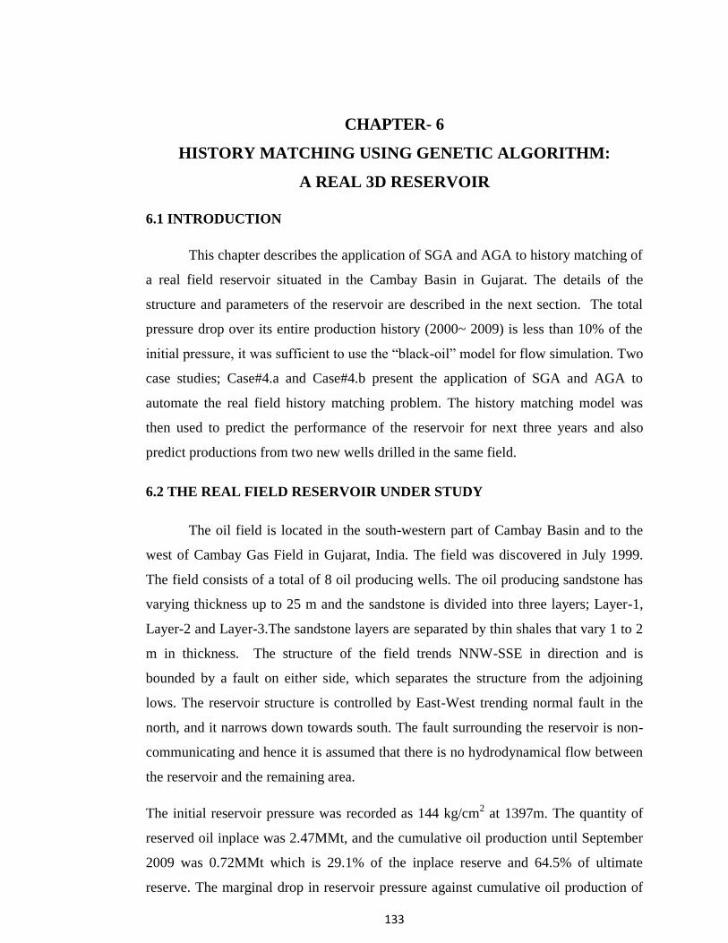
point pressure. Hence the model shows constant producing GOR. The grid bottom
structure 3D real reservoir is shown in Figure 6.1.
Fig 6.1. 3D view of grid bottom structure of real reservoir
The field started producing through the wells Well-1, and Well-2 from February, 2000
and December, 2000 respectively. The initial reservoir pressure recorded at Well-1
was 144.6 kg/cm2 at 1385m. The cumulative productions of oil, gas and water from
Well-1 till September 2009 are 0.156MMt, 8.1MMm3, and 7.2 MMm
3, respectively.
Subsequently, the other wells (Well-3 - Well-8) were drilled and put on production in
different years until 2009. The producing wells; Well- 3 and Well- 5 are perforated in
Layer- 1 and Layer- 2; while Well- 1; Well-2; Well- 4; and Well- 6 are perforated
through Layer-2 and Layer-3.
The case studies carried out here consider six oil producing wells (Well-1 – Well-6)
from the total of 8 oil producing wells. The historical production is available for a
period of 9 years. For the case studies, 70 months’ historical productions for the period
of 2000 – 2005 were used for history matching using GA methodology and remaining
(m)
135
data till 2009 were used for validating the model and the technique. Well-7 and Well-8
were put on production in January 2009.
6.2.1 Inputs to CMG®- Builder
TM suit
The reservoir model is constructed by amalgamating many parameters such as
petrophysical data, geological structure (structural contour map, pay-sand thickness
map etc.,), grid definition (size and type), PVT properties, reservoir fluid properties,
well completion data, initial conditions etc.,. The reservoir rock, fluid, PVT
parameters and initial conditions used to built a reservoir model through CMG®-
BuilderTM
are produced in Tables 6.1 and 6.2.
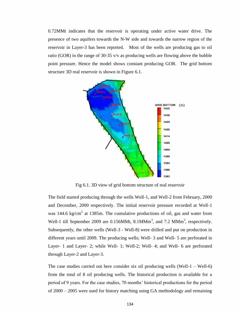
Table 6.1 Reservoir Model Parameters
Initial reservoir Pressure 144 kg/cm2
Datum Depth 1400 m
Porosity
Layer-1 0.21
Layer-2 0.22
Layer-3 0.23
Depth of Water Oil
Contact
Layer-1 1397 m
Layer-2 1401 m
Layer-3 1402 m
The relative permeability data have been generated using Corey’s correlation.
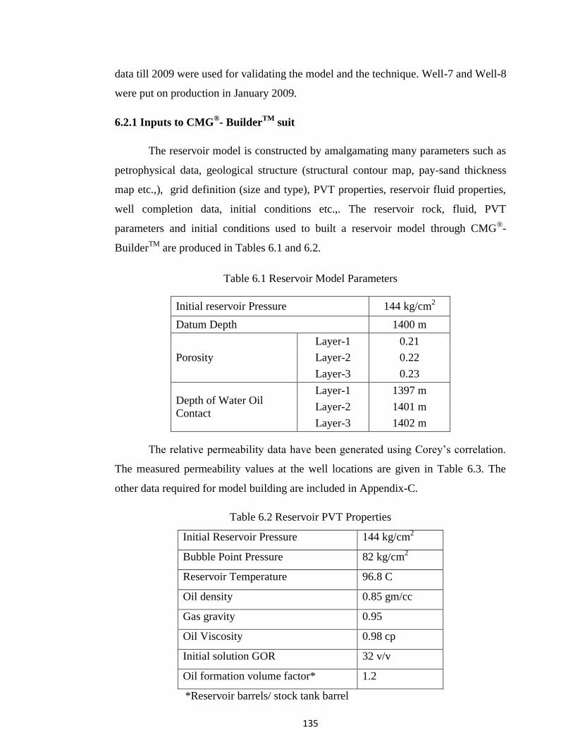
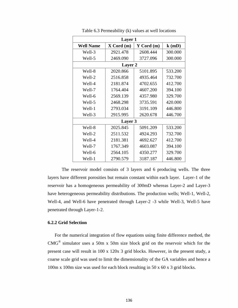
The measured permeability values at the well locations are given in Table 6.3. The
other data required for model building are included in Appendix-C.
Table 6.2 Reservoir PVT Properties
Initial Reservoir Pressure 144 kg/cm2
Bubble Point Pressure 82 kg/cm2
Reservoir Temperature 96.8 C
Oil density 0.85 gm/cc
Gas gravity 0.95
Oil Viscosity 0.98 cp
Initial solution GOR 32 v/v
Oil formation volume factor* 1.2
*Reservoir barrels/ stock tank barrel
136
Table 6.3 Permeability (k) values at well locations
Layer 1
Well Name X Cord (m) Y Cord (m) k (mD)
Well-3 2921.478 2608.444 300.000
Well-5 2469.090 3727.096 300.000
Layer 2
Well-8 2020.866 5101.895 533.200
Well-2 2516.858 4935.464 732.700
Well-4 2181.874 4702.655 412.700
Well-7 1764.404 4607.200 394.100
Well-6 2569.139 4357.980 329.700
Well-5 2468.298 3735.591 420.000
Well-1 2793.034 3191.109 446.800
Well-3 2915.995 2620.678 446.700
Layer 3
Well-8 2025.845 5091.209 533.200
Well-2 2511.532 4924.293 732.700
Well-4 2181.381 4692.627 412.700
Well-7 1767.349 4603.087 394.100
Well-6 2564.105 4350.277 329.700
Well-1 2790.579 3187.187 446.800
The reservoir model consists of 3 layers and 6 producing wells. The three
layers have different porosities but remain constant within each layer. Layer-1 of the
reservoir has a homogeneous permeability of 300mD whereas Layer-2 and Layer-3
have heterogeneous permeability distributions. The production wells; Well-1, Well-2,
Well-4, and Well-6 have penetrated through Layer-2 -3 while Well-3, Well-5 have
penetrated through Layer-1-2.
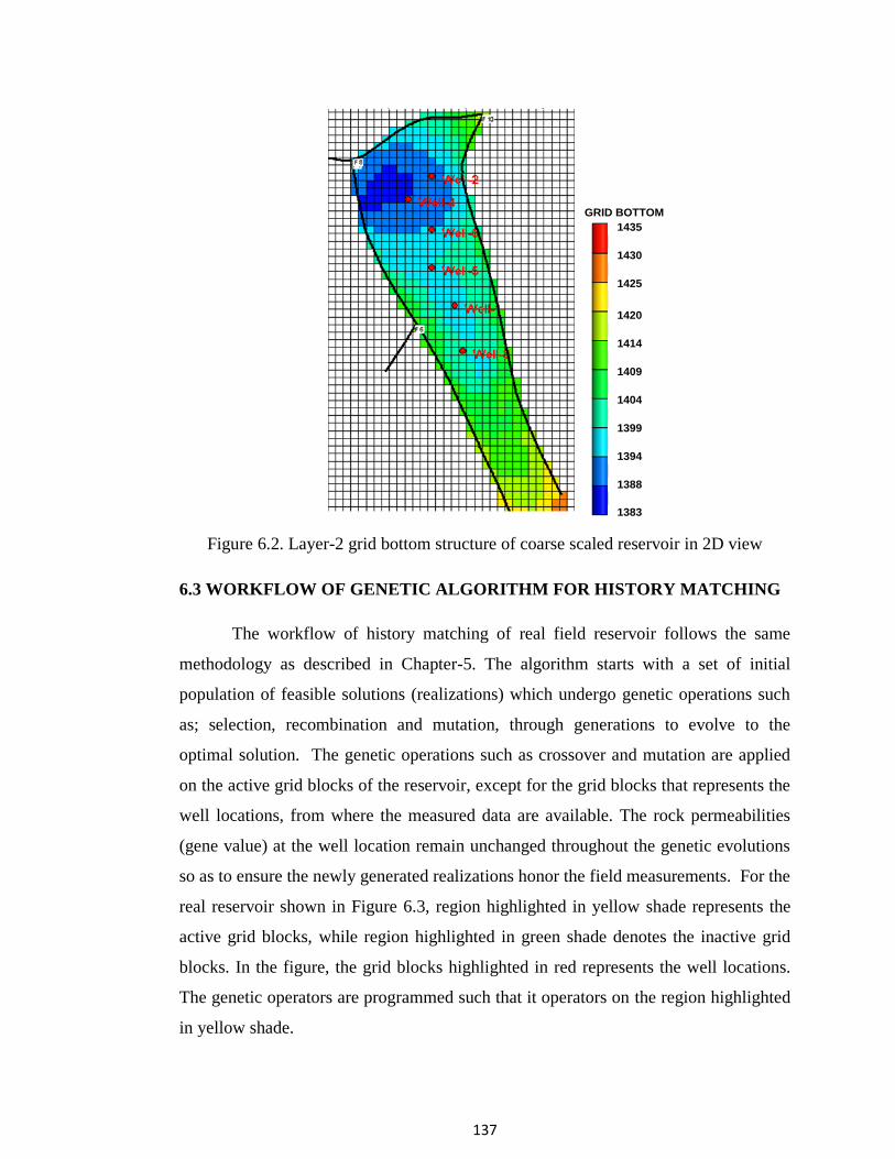
6.2.2 Grid Selection
For the numerical integration of flow equations using finite difference method, the
CMG® simulator uses a 50m x 50m size block grid on the reservoir which for the
present case will result in 100 x 120x 3 grid blocks. However, in the present study, a
coarse scale grid was used to limit the dimensionality of the GA variables and hence a
100m x 100m size was used for each block resulting in 50 x 60 x 3 grid blocks.
137
1383
1388
1394
1399
1404
1409
1414
1425
1430
1435
1420
GRID BOTTOM
Figure 6.2. Layer-2 grid bottom structure of coarse scaled reservoir in 2D view
6.3 WORKFLOW OF GENETIC ALGORITHM FOR HISTORY MATCHING
The workflow of history matching of real field reservoir follows the same
methodology as described in Chapter-5. The algorithm starts with a set of initial
population of feasible solutions (realizations) which undergo genetic operations such
as; selection, recombination and mutation, through generations to evolve to the
optimal solution. The genetic operations such as crossover and mutation are applied
on the active grid blocks of the reservoir, except for the grid blocks that represents the
well locations, from where the measured data are available. The rock permeabilities
(gene value) at the well location remain unchanged throughout the genetic evolutions
so as to ensure the newly generated realizations honor the field measurements. For the
real reservoir shown in Figure 6.3, region highlighted in yellow shade represents the
active grid blocks, while region highlighted in green shade denotes the inactive grid
blocks. In the figure, the grid blocks highlighted in red represents the well locations.
The genetic operators are programmed such that it operators on the region highlighted
in yellow shade.
138
(a) (b)
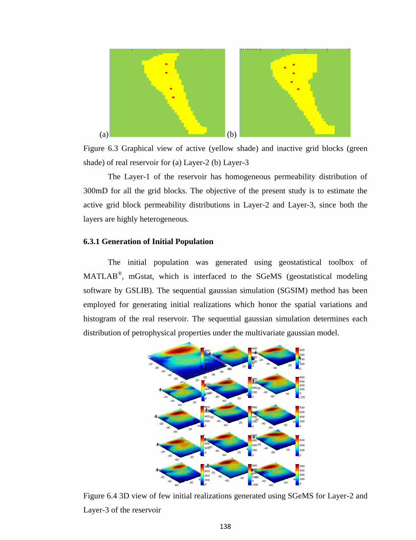
Figure 6.3 Graphical view of active (yellow shade) and inactive grid blocks (green
shade) of real reservoir for (a) Layer-2 (b) Layer-3
The Layer-1 of the reservoir has homogeneous permeability distribution of
300mD for all the grid blocks. The objective of the present study is to estimate the
active grid block permeability distributions in Layer-2 and Layer-3, since both the
layers are highly heterogeneous.
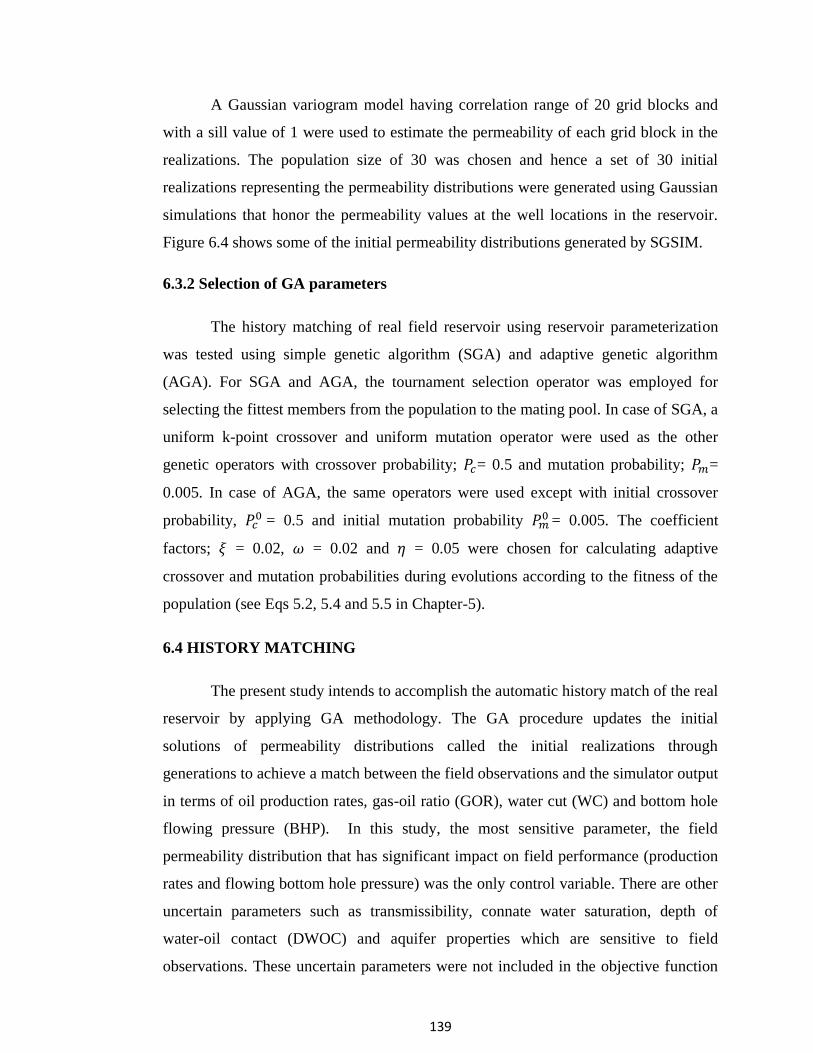
6.3.1 Generation of Initial Population
The initial population was generated using geostatistical toolbox of
MATLAB®, mGstat, which is interfaced to the SGeMS (geostatistical modeling
software by GSLIB). The sequential gaussian simulation (SGSIM) method has been
employed for generating initial realizations which honor the spatial variations and
histogram of the real reservoir. The sequential gaussian simulation determines each
distribution of petrophysical properties under the multivariate gaussian model.
Figure 6.4 3D view of few initial realizations generated using SGeMS for Layer-2 and
Layer-3 of the reservoir
1020
3040
50
-60
-50
-40
-30
-20
-10
-3-2-10
2040
-60
-40
-20
-3-2-10
2040
-60
-40
-20
-3-2-10
2040
-60
-40
-20
-3-2-10
2040
-60
-40
-20
-3-2-10
2040
-60
-40
-20
-3-2-10
2040
-60
-40
-20
-3-2-10
2040
-60
-40
-20
-3-2-10
2040
-60
-40
-20
-3-2-10
2040
-60
-40
-20
-3-2-10
2040
-60
-40
-20
-3-2-10
2040
-60
-40
-20
-3-2-10
2040
-60
-40
-20
-3-2-10
2040
-60
-40
-20
-3-2-10
2040
-60
-40
-20
-3-2-10
2040
-60
-40
-20
-3-2-10
20
40
-60
-40
-20
-3-2-10
2040
-60
-40
-20
-3-2-10
2040
-60
-40
-20
-3-2-10
2040
-60
-40
-20
-3-2-10
2040
-60
-40
-20
-3-2-10
2040
-60
-40
-20
-3-2-10
2040
-60
-40
-20
-3-2-10
2040
-60
-40
-20
-3-2-10
2040
-60
-40
-20
-3-2-10
2040
-60
-40
-20
-3-2-10
2040
-60
-40
-20
-3-2-10
2040
-60
-40
-20
-3-2-10
2040
-60
-40
-20
-3-2-10
2040
-60
-40
-20
-3-2-10
0
200
400
600
0
200
400
600
800
0
200
400
600
0
200
400
600
800
0
200
400
600
800
0
200
400
600
800
0
200
400
600
800
0
200
400
600
800
-200
0
200
400
600
800
0
200
400
600
800
-200
0
200
400
600
800
0
200
400
600
800
0
200
400
600
0
200
400
600
800
0
200
400
600
800
0
200
400
600
800
-200
0
200
400
600
800
0
200
400
600
800
0
200
400
600
0
200
400
600
800
-200
0
200
400
600
0
200
400
600
800
-200
0
200
400
600
0
200
400
600
800
0
200
400
600
800
0
200
400
600
800
0
200
400
600
800
-200
0
200
400
600
800
0
200
400
600
800
0
200
400
600
800
139
A Gaussian variogram model having correlation range of 20 grid blocks and
with a sill value of 1 were used to estimate the permeability of each grid block in the
realizations. The population size of 30 was chosen and hence a set of 30 initial
realizations representing the permeability distributions were generated using Gaussian
simulations that honor the permeability values at the well locations in the reservoir.
Figure 6.4 shows some of the initial permeability distributions generated by SGSIM.
6.3.2 Selection of GA parameters
The history matching of real field reservoir using reservoir parameterization
was tested using simple genetic algorithm (SGA) and adaptive genetic algorithm
(AGA). For SGA and AGA, the tournament selection operator was employed for
selecting the fittest members from the population to the mating pool. In case of SGA, a
uniform k-point crossover and uniform mutation operator were used as the other
genetic operators with crossover probability; = 0.5 and mutation probability; =
0.005. In case of AGA, the same operators were used except with initial crossover
probability, = 0.5 and initial mutation probability
= 0.005. The coefficient
factors; = 0.02, = 0.02 and = 0.05 were chosen for calculating adaptive
crossover and mutation probabilities during evolutions according to the fitness of the
population (see Eqs 5.2, 5.4 and 5.5 in Chapter-5).
6.4 HISTORY MATCHING
The present study intends to accomplish the automatic history match of the real
reservoir by applying GA methodology. The GA procedure updates the initial
solutions of permeability distributions called the initial realizations through
generations to achieve a match between the field observations and the simulator output
in terms of oil production rates, gas-oil ratio (GOR), water cut (WC) and bottom hole
flowing pressure (BHP). In this study, the most sensitive parameter, the field
permeability distribution that has significant impact on field performance (production
rates and flowing bottom hole pressure) was the only control variable. There are other
uncertain parameters such as transmissibility, connate water saturation, depth of
water-oil contact (DWOC) and aquifer properties which are sensitive to field
observations. These uncertain parameters were not included in the objective function
140
for estimation because of the computational constraints. However, some these are
adjusted manually as required.
6.4.1 Objective Function
The objective of this study to find the optimal field permeability distribution in
Layer-2 and 3 that minimizes the difference between the field observations and the
simulator output. The objective function is formulated based on Eq. 5.1 taking into
account the type of field observations, number of wells, and time period etc. In this
case study the field data comprises oil production rate, GOR, water cut and BHP from
all 6 producing wells over a period of 6 years (70 months) of production history (Mar,
2000 ~ Dec, 2005). Hence the objective function is expressed as
∑ ∑ (
)
(
)
(
)
(
)
(6.1)
where subscripts denote the number of wells and time period respectively;
and are the field observations and corresponding CMG
® simulator outputs in
terms of monthly oil production rate, GOR, WC and BHP. was minimized using
GA and search was terminated when successive iterations produced essentially same
values of the objective function.
6.5 RESULTS AND DISCUSSION
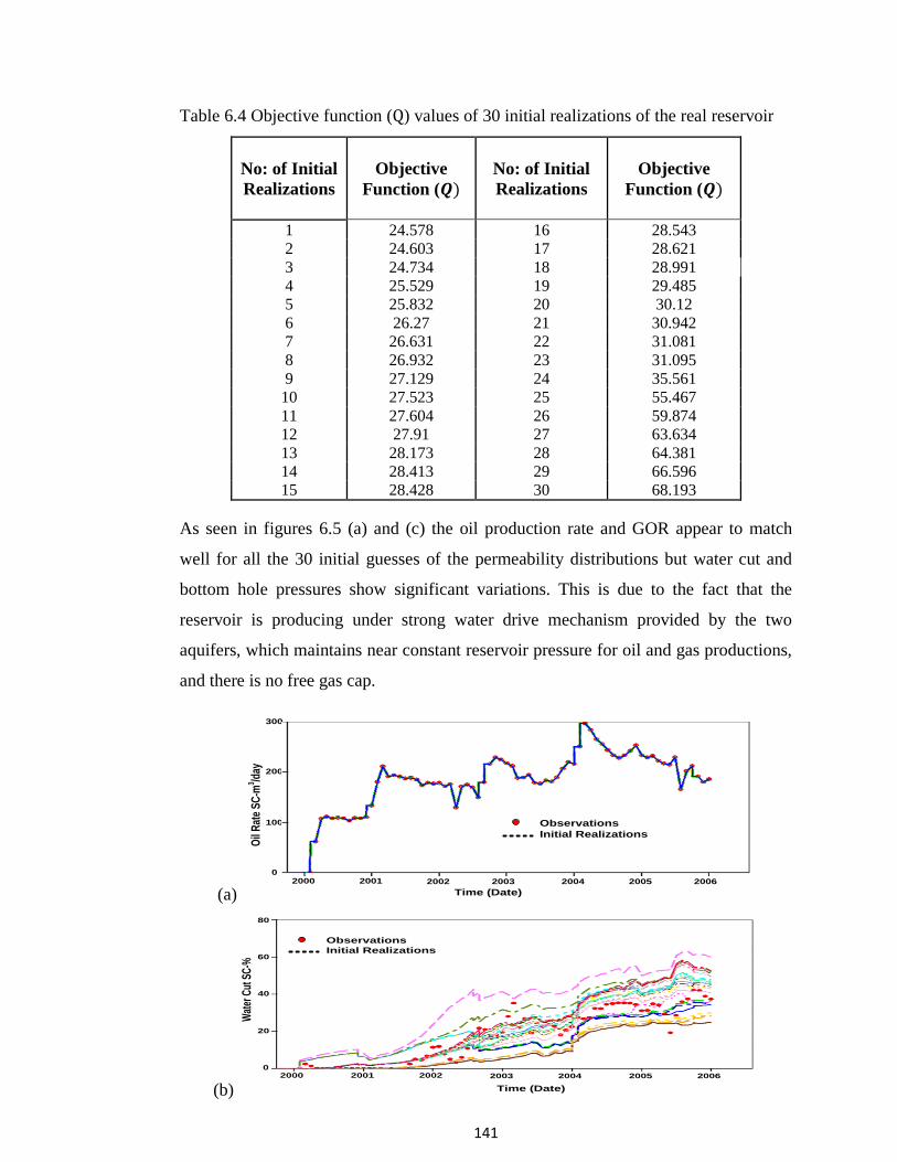
The objective function values of the initial realizations representing the field
permeability distributions are presented in Table 6.4. The minimum and maximum
objective function value ranges between 24.58 ~ 68.19 with the average value for
being 35.096. The oil production rates (m3/day), water cut -%, GOR (m
3/m
3)
and BHP (kg/cm2) for the entire field resulted from the initial realizations is shown in
Figure 6.5. Also included in this figure are field observations for comparison.
141
Table 6.4 Objective function ( ) values of 30 initial realizations of the real reservoir
No: of Initial
Realizations
Objective
Function (
No: of Initial
Realizations
Objective
Function (
1 24.578 16 28.543
2 24.603 17 28.621
3 24.734 18 28.991
4 25.529 19 29.485
5 25.832 20 30.12
6 26.27 21 30.942
7 26.631 22 31.081
8 26.932 23 31.095
9 27.129 24 35.561
10 27.523 25 55.467
11 27.604 26 59.874
12 27.91 27 63.634
13 28.173 28 64.381
14 28.413 29 66.596
15 28.428 30 68.193
As seen in figures 6.5 (a) and (c) the oil production rate and GOR appear to match
well for all the 30 initial guesses of the permeability distributions but water cut and
bottom hole pressures show significant variations. This is due to the fact that the
reservoir is producing under strong water drive mechanism provided by the two
aquifers, which maintains near constant reservoir pressure for oil and gas productions,
and there is no free gas cap.
(a)
0
100
200
300
2000 2001 2002 2003 2004 2005 2006
Time (Date)
Oil
Rat
e S
C-m
3 /day
Observations
Initial Realizations
(b)
0
20
40
60
80
2000 2001 2002 2003 2004 2005 2006
Time (Date)
Wat
er C
ut S
C-%
Observations
Initial Realizations

142
(c)
120
100
0
20
40
60
80
2000 2001 2002 2003 2004 2005 2006
Time (Date)
Gas
Oil
ratio
(m3 /m
3 ) Observations
Initial Realizations
(d)
120
130
140
150
2000 2001 2002 2003 2004 2005 2006
Time (Date)
Bot
tom
Hol
e Fl
owin
g P
ress
ure
Kg/
cm2
Observations
Initial Realizations
Figure 6.5. Comparison between the field observations and the simulator output
generated from 30 initial realizations (a) Oil production rate SC (m3/day) (b) GOR
(m3/m3) (c) Water cut SC- % (d) BHP (kg/cm2)
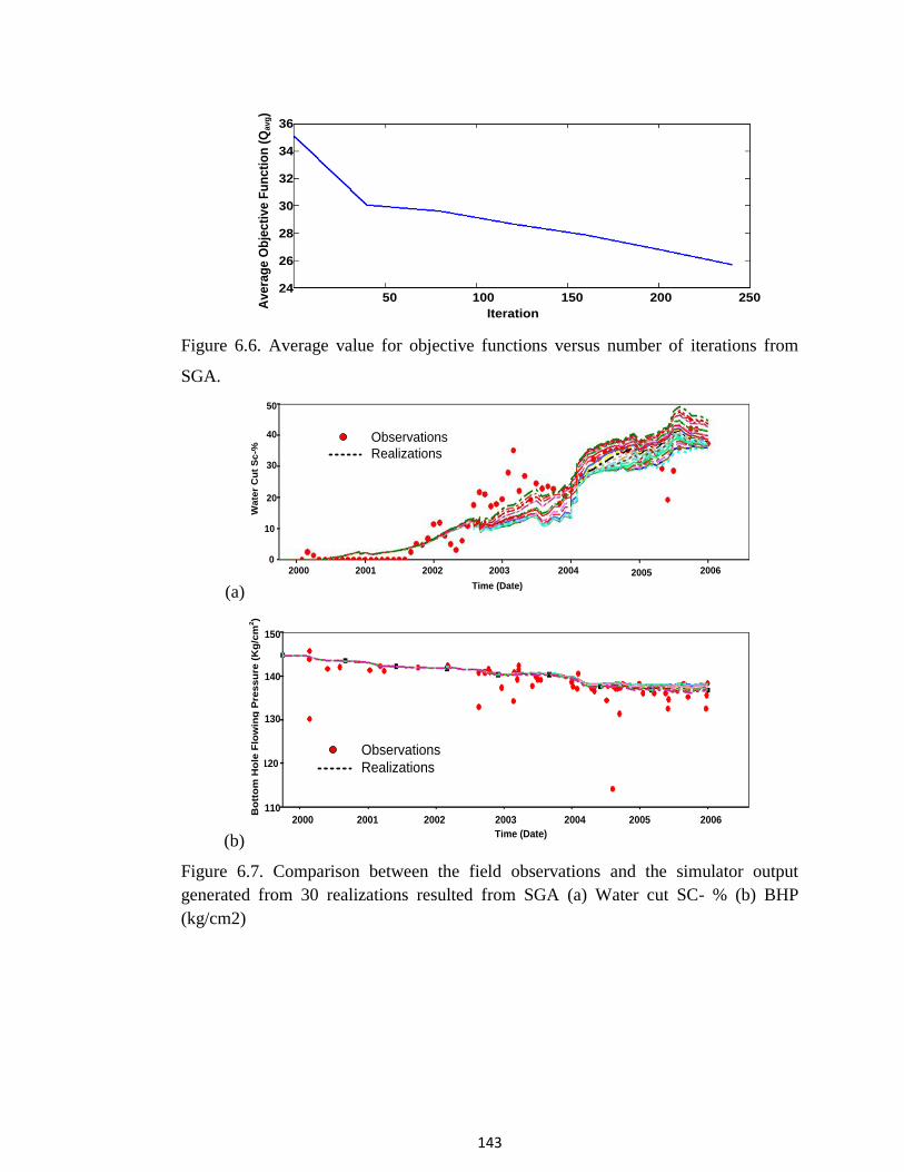
6.5.1 Results from SGA (Case#4.a)
The objective function values of the realizations resulting from SGA for the real
reservoir after every 40 iterations are presented in Table 6.5. The SGA search was
terminated after 240 iterations which resulted in an average value for
minimum value of = 19.98 (range 19.98 ~ 54.34). The objective function values
resulting from SGA do not appear to be very small when compared to the initial
realizations values. However, the water cut and BHP showed better match with the
field data. The variation of with iterations numbers is shown in Figure 6.6. The
comparison between the observed and simulator output from the 30 realizations
resulted from SGA in terms of WC and BHP is shown in Figure 6.7.
143
Iteration
Av
era
ge
Ob
jec
tiv
e F
un
cti
on
(Q
av
g)
50 100 200 25015024
26
28
30
32
34
36
Figure 6.6. Average value for objective functions versus number of iterations from
SGA.
(a)
50
10
0
Time (Date)
Wa
ter
Cu
t S
c-%
20
30
40
2000 20042001 2002 2003 2005 2006
Observations
Realizations
(b)
120
110
Time (Date)
Bo
tto
m H
ole
Flo
win
g P
res
su
re (
Kg
/cm
2)
130
140
150
2000 20042001 2002 2003 2005 2006
Observations
Realizations
Figure 6.7. Comparison between the field observations and the simulator output
generated from 30 realizations resulted from SGA (a) Water cut SC- % (b) BHP
(kg/cm2)
144
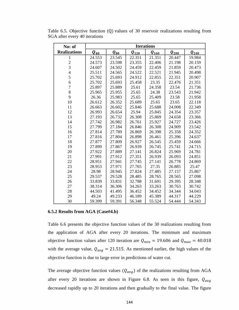
Table 6.5. Objective function ( of 30 reservoir realizations resulting from
SGA after every 40 iterations
No: of
Realizations
Iterations
1 24.553 23.545 22.351 21.351 20.447 19.984
2 24.573 23.598 23.355 22.406 21.198 20.159
3 24.607 24.502 24.459 22.459 21.859 20.473
4 25.511 24.565 24.522 22.521 21.945 20.498
5 25.702 25.693 24.912 22.855 22.351 20.907
6 25.702 25.693 25.458 23.35 22.476 21.351
7 25.897 25.889 25.61 24.358 23.54 21.736
8 25.965 25.955 25.65 24.38 23.543 21.942
9 26.36 25.983 25.65 25.409 23.58 21.958
10 26.612 26.352 25.689 25.65 23.65 22.118
11 26.663 26.602 25.846 25.688 24.008 22.349
12 26.993 26.654 25.94 25.845 24.354 23.357
13 27.193 26.732 26.308 25.869 24.658 23.366
14 27.742 26.982 26.761 25.927 24.727 23.426
15 27.799 27.184 26.846 26.308 24.909 23.542
16 27.814 27.789 26.869 26.398 25.358 24.352
17 27.816 27.804 26.898 26.461 25.396 24.637
18 27.877 27.809 26.927 26.545 25.459 24.666
19 27.899 27.867 26.939 26.745 25.741 24.715
20 27.922 27.889 27.141 26.824 25.969 24.781
21 27.991 27.912 27.351 26.939 26.093 24.851
22 28.951 27.941 27.745 27.141 26.778 24.869
23 28.953 27.971 27.765 27.35 26.885 25.47
24 28.98 28.945 27.824 27.485 27.157 25.867
25 29.537 29.528 28.485 28.765 28.565 27.098
26 33.839 33.831 32.788 31.691 29.395 28.348
27 38.314 36.306 34.263 33.263 30.763 30.742
28 44.503 41.495 36.452 34.452 34.344 34.043
29 49.24 49.233 46.189 45.389 44.317 44.229
30 59.399 59.391 56.348 55.524 54.444 54.343
6.5.2 Results from AGA (Case#4.b)
Table 6.6 presents the objective function values of the 30 realizations resulting from
the application of AGA after every 20 iterations. The minimum and maximum
objective function values after 120 iteration are and
with the average value, . As mentioned earlier, the high values of the
objective function is due to large error in predictions of water cut.
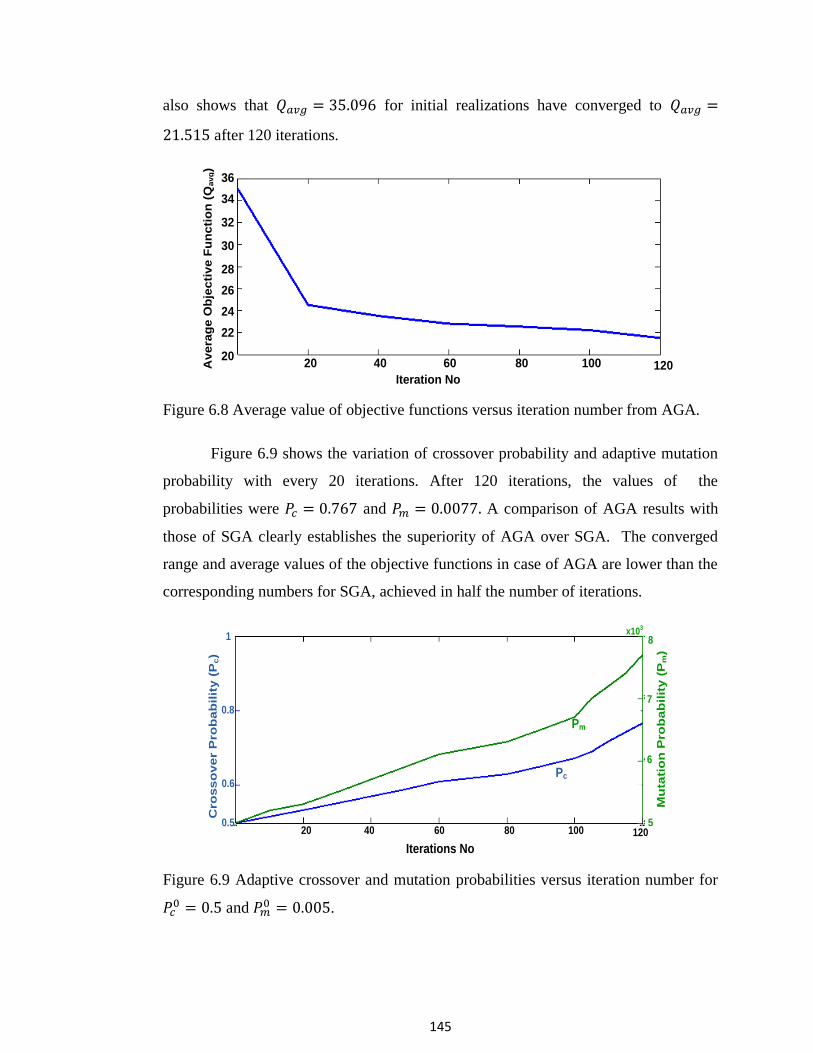
The average objective function values of the realizations resulting from AGA
after every 20 iterations are shown in Figure 6.8. As seen in this figure,
decreased rapidly up to 20 iterations and then gradually to the final value. The figure
145
also shows that for initial realizations have converged to
after 120 iterations.
Iteration No
Av
era
ge
Ob
jec
tiv
e F
un
cti
on
(Q
av
g)
20 40 80 10060
24
26
28
30
32
34
36
120
22
20
Figure 6.8 Average value of objective functions versus iteration number from AGA.
Figure 6.9 shows the variation of crossover probability and adaptive mutation
probability with every 20 iterations. After 120 iterations, the values of the
probabilities were and A comparison of AGA results with
those of SGA clearly establishes the superiority of AGA over SGA. The converged
range and average values of the objective functions in case of AGA are lower than the
corresponding numbers for SGA, achieved in half the number of iterations.
Cro
ss
ov
er
Pro
ba
bilit
y (
Pc)
6
7
8
Mu
tati
on
Pro
ba
bilit
y (
Pm
)
5
x103
1
0.8
0.6
0.5
Iterations No
20 40 80 100 12060
Pm
Pc
Figure 6.9 Adaptive crossover and mutation probabilities versus iteration number for
and
.
146
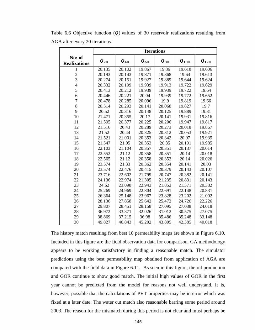
Table 6.6 Objective function ( of 30 reservoir realizations resulting from
AGA after every 20 iterations
Iterations
No: of
Realizations
1 20.135 20.102 19.867 19.86 19.618 19.606
2 20.193 20.143 19.871 19.868 19.64 19.613
3 20.274 20.151 19.927 19.889 19.644 19.624
4 20.332 20.199 19.939 19.913 19.722 19.629
5 20.413 20.212 19.939 19.939 19.722 19.64
6 20.446 20.221 20.04 19.939 19.772 19.652
7 20.478 20.285 20.096 19.9 19.819 19.66
8 20.514 20.293 20.141 20.068 19.827 19.7
9 20.52 20.316 20.148 20.125 19.889 19.81
10 21.471 20.355 20.17 20.141 19.931 19.816
11 21.505 20.377 20.225 20.206 19.947 19.817
12 21.516 20.43 20.289 20.273 20.018 19.867
13 21.52 20.44 20.325 20.312 20.053 19.921
14 21.521 21.001 20.353 20.342 20.07 19.935
15 21.547 21.05 20.353 20.35 20.101 19.985
16 22.103 21.104 20.357 20.351 20.137 20.014
17 22.552 21.12 20.358 20.351 20.14 20.018
18 22.565 21.12 20.358 20.353 20.14 20.026
19 23.574 21.33 20.362 20.354 20.141 20.03
20 23.574 22.476 20.415 20.379 20.143 20.107
21 23.716 22.602 21.799 20.747 20.382 20.141
22 24.136 22.974 21.305 21.235 20.831 20.143
23 24.62 23.098 22.943 21.852 21.371 20.382
24 25.269 24.969 22.804 22.691 22.148 20.831
25 26.364 25.148 23.967 23.828 23.202 21.002
26 28.136 27.858 25.642 25.472 24.726 22.226
27 29.807 28.451 28.158 27.095 27.038 24.018
28 36.972 33.371 32.026 31.012 30.575 27.075
29 38.869 37.215 36.98 35.486 35.248 33.148
30 49.827 46.843 45.202 43.805 42.385 40.018
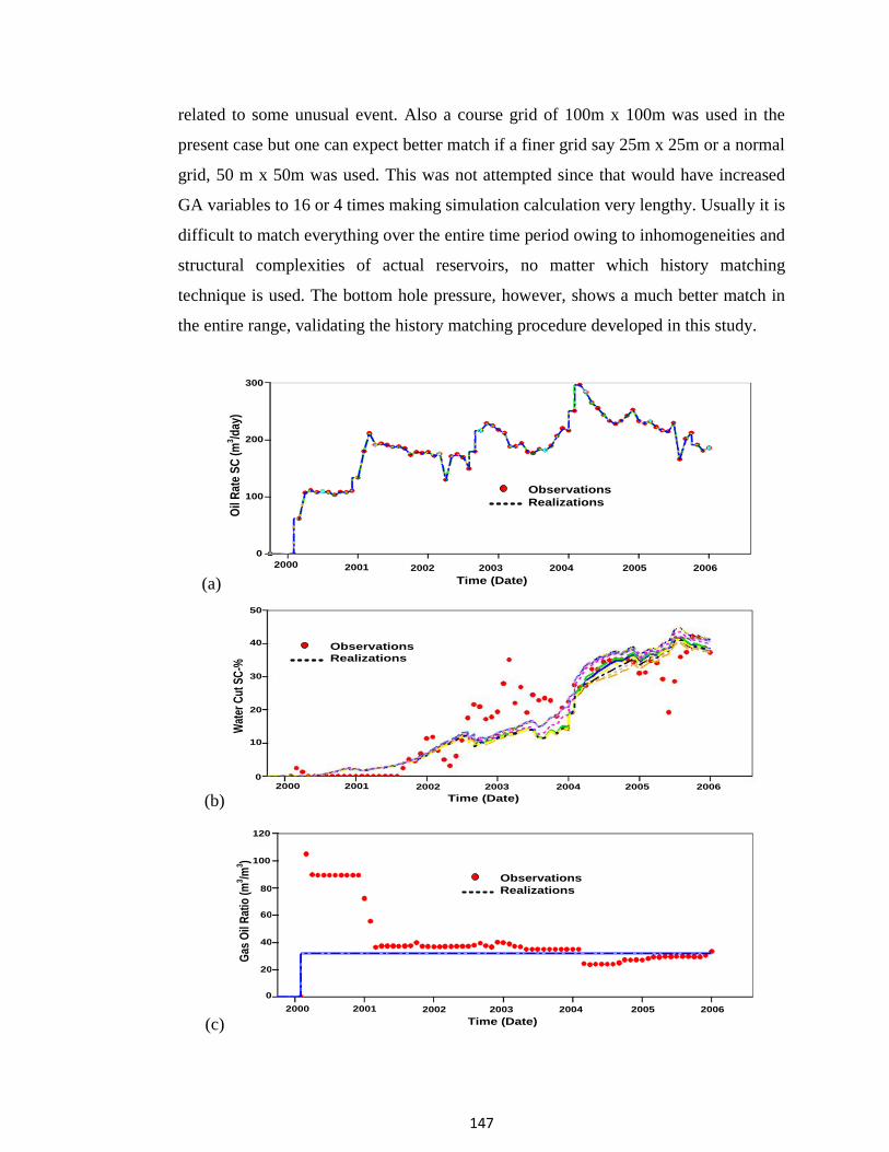
The history match resulting from best 10 permeability maps are shown in Figure 6.10.
Included in this figure are the field observation data for comparison. GA methodology
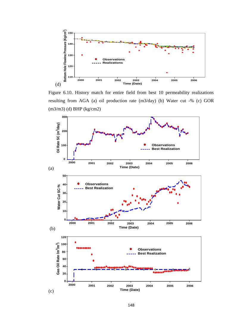
appears to be working satisfactory in finding a reasonable match. The simulator
predictions using the best permeability map obtained from application of AGA are
compared with the field data in Figure 6.11. As seen in this figure, the oil production
and GOR continue to show good match. The initial high values of GOR in the first
year cannot be predicted from the model for reasons not well understand. It is,
however, possible that the calculations of PVT properties may be in error which was
fixed at a later date. The water cut match also reasonable barring some period around
2003. The reason for the mismatch during this period is not clear and must perhaps be
147
related to some unusual event. Also a course grid of 100m x 100m was used in the
present case but one can expect better match if a finer grid say 25m x 25m or a normal
grid, 50 m x 50m was used. This was not attempted since that would have increased
GA variables to 16 or 4 times making simulation calculation very lengthy. Usually it is
difficult to match everything over the entire time period owing to inhomogeneities and
structural complexities of actual reservoirs, no matter which history matching
technique is used. The bottom hole pressure, however, shows a much better match in
the entire range, validating the history matching procedure developed in this study.
(a)
2000
2001 2002 2003 2004 2005 2006
Time (Date)
Oil
Rat
e S
C (
m3 /d
ay)
100
200
300
0
2000
Observations
Realizations
(b)
50
0
10
20
30
40
2000 2001 2002 2003 2004 2005 2006
Time (Date)
Wat
er C
ut S
C-%
Observations
Realizations
(c)
120
80
20
60
40
0
100
2000 2001 2002 2003 2004 2005 2006
Time (Date)
Gas
Oil
Rat
io (
m3 /m
3 )
Observations
Realizations
148
(d)
120
2000 2001 2002 2003 2004 2005 2006
Time (Date)
Bo
tto
m H
ole
Flo
win
g P
ress
ure
(K
g/c
m2 )
130
140
150
110
Observations
Realizations
Figure 6.10. History match for entire field from best 10 permeability realizations
resulting from AGA (a) oil production rate (m3/day) (b) Water cut -% (c) GOR
(m3/m3) (d) BHP (kg/cm2)
(a)
2001 2002 2003 2004 2005 2006
Time (Date)
Oil R
ate
SC
(m
3/d
ay)
100
200
300
0
2000
Observations
Best Realization
(b)
2001 2002 2003 2004 2005 2006
Time (Date)
Wa
ter
Cu
t S
C-%
2000
50
30
10
20
0
40 Observations
Best Realization
(c)
2001 2002 2003 2004 2005 2006
Time (Date)
Ga
s O
il R
ate
(m
3/m
3)
2000
120
80
20
60
40
0
100
Observations
Best Realization
149
(d)
2001 2002 2003 2004 2005 2006
Time (Date)
2000
140
120
130
110
150
Bo
tto
m H
ole
Flo
win
g P
res
su
re
(Kg
/cm
2)
Observations
Best Realization
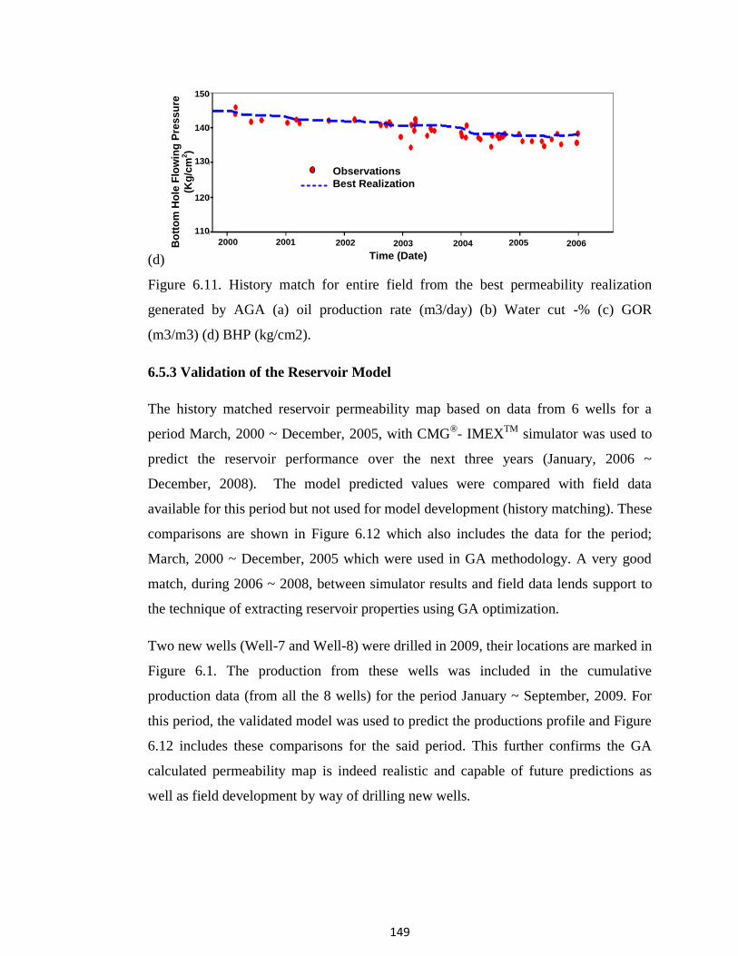
Figure 6.11. History match for entire field from the best permeability realization
generated by AGA (a) oil production rate (m3/day) (b) Water cut -% (c) GOR
(m3/m3) (d) BHP (kg/cm2).
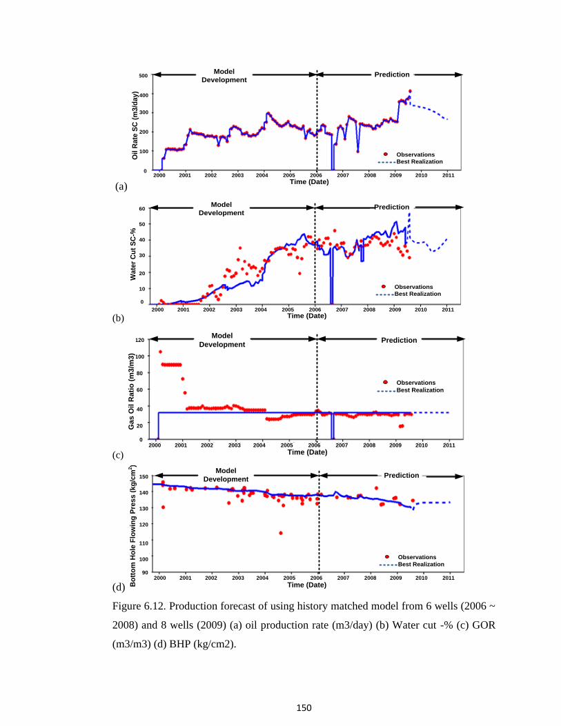
6.5.3 Validation of the Reservoir Model
The history matched reservoir permeability map based on data from 6 wells for a
period March, 2000 ~ December, 2005, with CMG®- IMEX
TM simulator was used to
predict the reservoir performance over the next three years (January, 2006 ~
December, 2008). The model predicted values were compared with field data
available for this period but not used for model development (history matching). These
comparisons are shown in Figure 6.12 which also includes the data for the period;
March, 2000 ~ December, 2005 which were used in GA methodology. A very good
match, during 2006 ~ 2008, between simulator results and field data lends support to
the technique of extracting reservoir properties using GA optimization.
Two new wells (Well-7 and Well-8) were drilled in 2009, their locations are marked in
Figure 6.1. The production from these wells was included in the cumulative
production data (from all the 8 wells) for the period January ~ September, 2009. For
this period, the validated model was used to predict the productions profile and Figure
6.12 includes these comparisons for the said period. This further confirms the GA
calculated permeability map is indeed realistic and capable of future predictions as
well as field development by way of drilling new wells.
150
(a)
Observations
Best Realization
Model
DevelopmentPrediction
2000 2001 2002 2003 2004 2005 2006 2007 2008 2009 2010 2011
Time (Date)
0
500
400
300
200
100
Oil R
ate
SC
(m
3/d
ay
)
(b)
Observations
Best Realization
Model
DevelopmentPrediction
2000 2001 2002 2003 2004 2005 2006 2007 2008 2009 2010 2011
Time (Date)
10
30
20
40
50
60
0
Wa
ter
Cu
t S
C-%
(c)
Observations
Best Realization
Model
DevelopmentPrediction
2000 2001 2002 2003 2004 2005 2006 2007 2008 2009 2010 2011
Time (Date)
120
0
100
80
60
40
20Ga
s O
il R
ati
o (
m3
/m3)
(d) Bo
tto
m H
ole
Flo
win
g P
res
s (
kg
/cm
2)
Observations
Best Realization
Model
DevelopmentPrediction
2000 2001 2002 2003 2004 2005 2006 2007 2008 2009 2010 2011
Time (Date)
150
90
140
130
120
110
100
Figure 6.12. Production forecast of using history matched model from 6 wells (2006 ~
2008) and 8 wells (2009) (a) oil production rate (m3/day) (b) Water cut -% (c) GOR
(m3/m3) (d) BHP (kg/cm2).
151
(1)
Observations
Best Realization
Observations
Best Realization
Observations
Best Realization
(a) (b)
(c) (d)
Observations
Best Realization
Well-1
BH
P (
kg/c
m2)
(2)
Observations
Best Realization
Observations
Best Realization
Observations
Best Realization
(a) (b)
(c) (d)
Observations
Best Realization
Well-2
BH
P (
kg/c
m2)
(3)
Observations
Best Realization
Observations
Best Realization
Observations
Best Realization
(a) (b)
(c) (d)
Observations
Best
Realization
Well-3
BH
P (
kg/c
m2)
152
(4)
Observations
Best Realization
Observations
Best Realization
Observations
Best Realization
(a) (b)
(c) (d)
Observations
Best
Realization
Well-4
BH
P (
kg/c
m2)
(5)
Observations
Best RealizationObservations
Best Realization
Observations
Best Realization
Observations
Best Realization
Well-5
BH
P (
kg/c
m2)
(6)
Observations
Best Realization
Observations
Best Realization
Observations
Best Realization
(a) (b)
(c) (d)
Observations
Best Realization
Well-6
BH
P (
kg/c
m2)
153
(7)
Observations
Best Realization
Observations
Best Realization
Observations
Best Realization
(a) (b)
(c) (d)
Observations
Best Realization
Well-7
BH
P (
kg/c
m2
)
(8)
Observations
Best Realization
Observations
Best Realization
Observations
Best Realization
(a) (b)
(c) (d)
Observations
Best Realization
Well-8
BH
P (
kg/c
m2
)
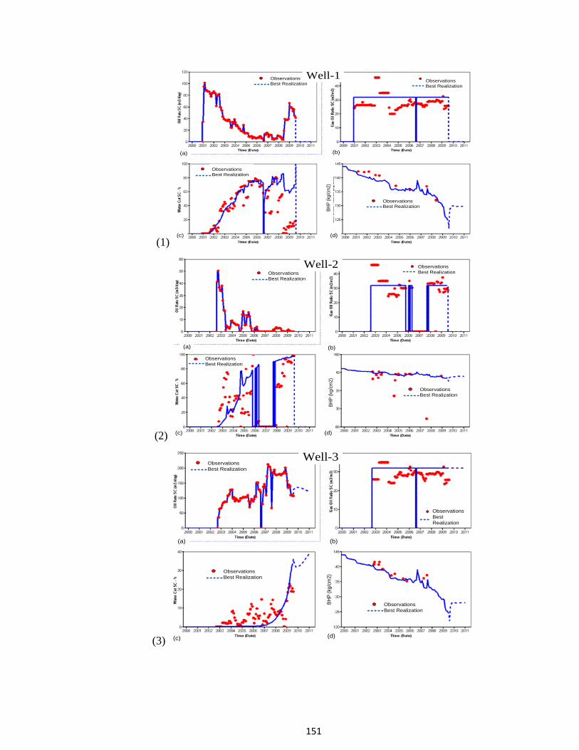
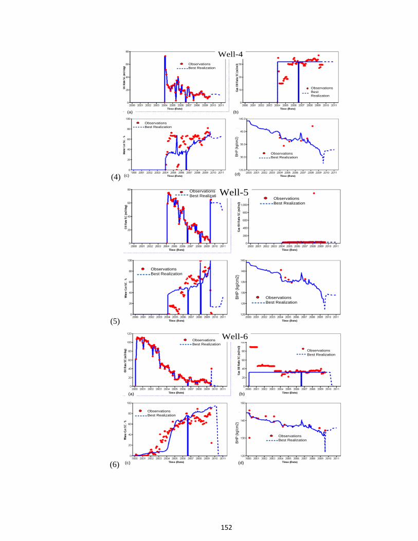
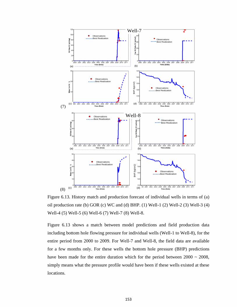
Figure 6.13. History match and production forecast of individual wells in terms of (a)
oil production rate (b) GOR (c) WC and (d) BHP. (1) Well-1 (2) Well-2 (3) Well-3 (4)
Well-4 (5) Well-5 (6) Well-6 (7) Well-7 (8) Well-8.
Figure 6.13 shows a match between model predictions and field production data
including bottom hole flowing pressure for individual wells (Well-1 to Well-8), for the
entire period from 2000 to 2009. For Well-7 and Well-8, the field data are available
for a few months only. For these wells the bottom hole pressure (BHP) predictions
have been made for the entire duration which for the period between 2000 ~ 2008,
simply means what the pressure profile would have been if these wells existed at these
locations.