chapter 6 portfolio selection - information and...

CHAPTER – 6

PORTFOLIO SELECTION

Feasible set of portfolios

Efficient set of portfolios

Selection of optimal portfolio

Portfolio selection models:

Markowitz Model-

Limitations of Markowitz model

Single Index Model-

Measuring security return and risk under Single Index Model

Measuring portfolio return and risk under Single Index Model

Multi-Index Model

Portfolio Selection 170

PORTFOLIO SELECTION:

The objective of every rational investor is to maximise his returns and

minimise the risk. Diversification is the method adopted for reducing risk. It

essentially results in the construction of portfolios. The proper goal of portfolio

construction would be to generate a portfolio that provides the highest return and the

lowest risk. Such a portfolio would be known as the optimal portfolio. The process

of finding the optimal portfolio is described as portfolio selection. The conceptual

framework and analytical tools for determining the optimal portfolio in disciplined

and objective manner have been provided by Harry Markowitz in his pioneering

work on portfolio analysis described in 1952 Journal of Finance article and

subsequent book in 1959. His method of portfolio selection has come to be known

as the Markowitz model. In fact, Markowitz‘s work marks the beginning of what is

known today as modern portfolio theory.

Feasible set of portfolios:

With a limited number of securities an investor can create a very large

number of portfolios by combining these securities in different proportions. These

constitute the feasible set of portfolios in which the investor can possibly invest.

This is also known as the portfolio opportunity set.

Each portfolio in the opportunity set is characterised by an expected return

and a measure of risk, viz., variance or standard deviation of returns. Not every

portfolio in the portfolio opportunity set is of interest to an investor. In the

opportunity set some portfolios will obviously be dominated by others. A portfolio

will dominate another if it has either a lower standard deviation and the same

expected return as the other, or a higher expected return and the same standard

deviation as the other. Portfolios that are dominated by other portfolios are known as

inefficient portfolios. An investor would not be interested in all the portfolios in the

opportunity set. He would be interested only in the efficient portfolios.

Efficient set of portfolios:

Let us consider various combinations of securities and designate them as

portfolios 1 to n. The expected returns of these portfolios may be worked out. The


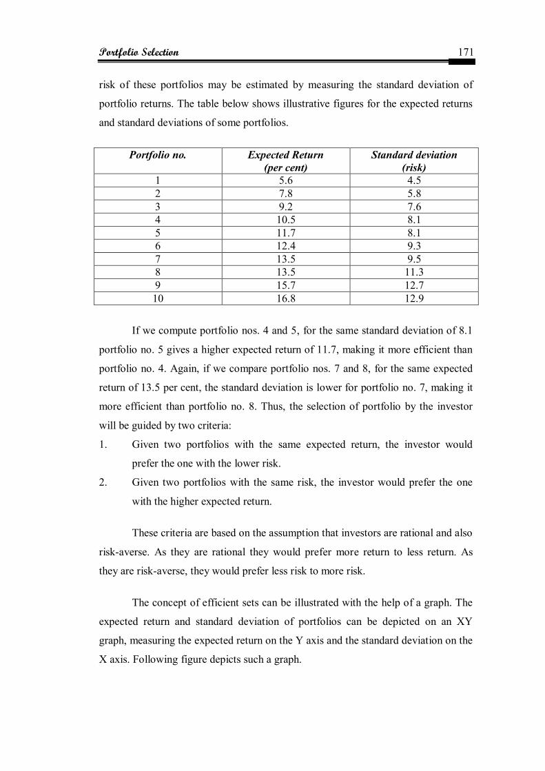
risk of these portfolios may be estimated by measuring the standard deviation of

portfolio returns. The table below shows illustrative figures for the expected returns

and standard deviations of some portfolios.

Portfolio no. Expected Return

(per cent)

Standard deviation

(risk)

1 5.6 4.5

2 7.8 5.8

3 9.2 7.6

4 10.5 8.1

5 11.7 8.1

6 12.4 9.3

7 13.5 9.5

8 13.5 11.3

9 15.7 12.7

10 16.8 12.9

If we compute portfolio nos. 4 and 5, for the same standard deviation of 8.1

portfolio no. 5 gives a higher expected return of 11.7, making it more efficient than

portfolio no. 4. Again, if we compare portfolio nos. 7 and 8, for the same expected

return of 13.5 per cent, the standard deviation is lower for portfolio no. 7, making it

more efficient than portfolio no. 8. Thus, the selection of portfolio by the investor

will be guided by two criteria:

1. Given two portfolios with the same expected return, the investor would

prefer the one with the lower risk.

2. Given two portfolios with the same risk, the investor would prefer the one

with the higher expected return.

These criteria are based on the assumption that investors are rational and also

risk-averse. As they are rational they would prefer more return to less return. As

they are risk-averse, they would prefer less risk to more risk.

The concept of efficient sets can be illustrated with the help of a graph. The

expected return and standard deviation of portfolios can be depicted on an XY

graph, measuring the expected return on the Y axis and the standard deviation on the

X axis. Following figure depicts such a graph.


As each possible portfolio in the opportunity set or feasible set of portfolios

has an expected return and standard deviation associated with it, each portfolio

would be represented by a single point in the risk-return space enclosed within the

two axes of the graph. The shaded area in the graph represents the set of all possible

portfolios that can be constructed from a given set of securities. This opportunity set

of portfolios takes a concave shape because it consists of portfolios containing

securities that are less than perfectly correlated with each other.

Diagram:

Consider portfolios F and E. Both the portfolios have the same expected

return but portfolio E has less risk. Hence, portfolio E would be preferred to

portfolio F. Now consider portfolios C and E. Both have the same risk, but portfolio

E offers more return for the same risk. Hence, portfolio E would be preferred to

portfolio C. Thus, for any point of risk-return space, an investor would like to move

as far as possible in the direction of increasing returns and also as far as possible in

the direction of decreasing risk. Effectively, he would be moving towards the left in

search of decreasing risk and upwards in search of increasing returns.

Feasible set of portfolios


Let us consider portfolios C and A. Portfolio C would be preferred to

portfolio A because it offers less risk for the same level of return. In the opportunity

set of portfolios represented in the diagram, portfolio C has the lowest risk compared

to all other portfolios. Here portfolio C in this diagram represents the global

minimum variance portfolio.

Comparing portfolios A and B, we find that portfolio B is preferable to

portfolio A because it offers higher return for the same level of risk. In this diagram,

point B represents the portfolio with the highest expected return among all the

portfolios in the feasible set.

Thus, we find that portfolios lying in the north-west boundary of the shaded

area are more efficient than all the portfolios in the interior of the shaded area. This

boundary of the shaded area is called the efficient frontier because it contains all the

efficient portfolios in the opportunity set. The set of portfolios lying between the

global minimum variance portfolio and the maximum return portfolio on the

efficient frontier represents the efficient set of portfolios. The efficient frontier is

shown separately in the following figure:

The efficient frontier


The efficient frontier is a concave curve in the risk-return space that extends

from the minimum variance portfolio to the maximum return portfolio.

Selection of optimal portfolio:

The portfolio selection problem is really the process of delineating the

efficient portfolios and then selecting the best portfolio from the set.

Rational investors will obviously prefer to invest in the efficient portfolios.

The particular portfolio that an individual investor will select from the efficient

frontier will depend on that investor‘s degree of aversion to risk. A highly risk

averse investor will hold a portfolio on the lower left hand segment of the efficient

frontier, while an investor who is not too risk averse will hold one on the upper

portion of the efficient frontier.

The selection of the optimal portfolio thus depends on the investor‘s risk

aversion, or conversely on his risk tolerance. This can be graphically represented

through a series of risk return utility curves or indifference curves. The indifference

curves of an investor are shown in the figure below. Each curve represents different

combinations of risk and return all of which are equally satisfactory to the concerned

investor. The investor is indifferent between the successive points in the curve. Each

successive curve moving upwards to the left represents a higher level of satisfaction

or utility. The investor‘s goal would be to maximise his utility by moving upto the

higher utility curve. The optimal portfolio for an investor would be the one at the

point of tangency between the efficient frontier and the risk-return utility or

indifference curve.

This is shown in the following figure. The point O‘ represents the optimal

portfolio.


Optimal portfolio

Markowitz used the technique of quadratic programming to identify the

efficient portfolios. Using the expected return and risk of each security under

consideration and the covariance estimates for each pair of securities, he calculated

risk and return for all possible portfolios. Then, for any specific value of expected

portfolio return, he determined the least risk portfolio using quadratic programming.

With another value of expected portfolio return, a similar procedure again gives the

minimum risk portfolio. The process is repeated with different values of expected

return, the resulting minimum risk portfolios constitute the set of efficient portfolios.

Limitations of Markowitz model:

1. Large number of input data required for calculations: An investor must

obtain estimates of return and variance of returns for all securities as also

covariances of returns for each pair of securities included in the portfolio. If

there are N securities in the portfolio, he would need N return estimates, N

variance estimates and N (N-1) / 2 covariance estimates, resulting in a total

of 2N + [N (N-1) / 2] estimates. For example, analysing a set of 200

securities would require 200 return estimates, 200 variance estimates and


19,900 covariance estimates, adding upto a total of 20,300 estimates. For a

set of 500 securities, the estimates would be 1,25,750. Thus, the number of

estimates required becomes large because covariances between each pair of

securities have to be estimated.

2. Complexity of computations required: The computations required are

numerous and complex in nature. With a given set of securities infinite number

of portfolios can be constructed. The expected returns and variances of returns

for each possible portfolio have to be computed. The identification of efficient

portfolios requires the use of quadratic programming which is a complex

procedure.

Because of the difficulties associated with the Markowitz model, it has found

little use in practical applications of portfolio analysis. Much simplification is

needed before the theory can be used for practical applications. Simplification is

needed in the amount and type of input data required to perform portfolio analysis;

simplification is also needed in the computational procedure used to select optimal

portfolios.

The simplification is achieved through index models. There are essentially two

types of index models:

Single index model

Multi-index model

The single index model is the simplest and the most widely used

simplification and may be regarded as being at one extreme point of a continuum,

with the Markowitz model at the other extreme point.

Multi-index models may be placed at the mid region of this continuum of

portfolio analysis techniques.

Single index model:

The basic notion underlying the single index model is that all stocks are

affected by movements in the stock market. Casual observation of share prices


reveals that when the market moves up, prices of most shares tend to increase. When

the market goes down, the prices of most shares tend to decline. This suggests that

one reason why security returns might be correlated and there is co-movement

between securities, is because of a common response to market changes. This co-

movement of stocks with a market index may be studied with the help of a simple

linear regression analysis, taking the returns on an individual security as the

dependent variable (Ri) and the returns on the market index (Rm) as the independent

variable.

The return of an individual security is assumed to depend on the return on

the market index. The return of an individual security may be expressed as:

Where

= Component of security i‘s return that is independent of the market‘s

performance.

= Rate of return on the market index.

= Constant that measures the expected change in given a change in .

= Error term representing the random or residual return.

This equation breaks the return on a stock into two components, one part due

to the market and the other part independent of the market. The beta parameter in the

equation, , measures how sensitive a stock‘s return is to the return on the market

index. It indicates how extensively the return of a security will vary with changes in

the market return.

The alpha parameter indicates what the return of the security would be

when the market return is zero. The positive alpha represents a sort of bonus return

and would be a highly desirable aspect of a security, whereas a negative alpha

represents a penalty to the investor and is an undesirable aspect of a security.

The final term in the equation, , is the unexpected return resulting from

influences not identified by the model. It is referred to as the random or residual

return. It may take on any value, but over a large number of observations it will

average out to zero.


William Sharpe, who tried to simplify the data inputs and data tabulation

required for the Markowitz model of portfolio analysis, suggested that a satisfactory

simplification would be achieved by abandoning the covariance of each security

with each other security and substituting in its place the relationship of each security

with a market index as measured by the single index model. This is known as Sharpe

index model.

In the place of [N (N – 1) / 2] covariances required for the Markowitz model,

Sharpe model would requires only N measures of beta coefficients.

Measuring security return and risk under Single Index Model:

Using the single index model, expected return of an individual security may

be expressed as:

The return of the security is a combination of two components:

(a) A specific return component represented by the alpha of the security; and

(b) A market related return component represented by the term .

The residual return disappears from the expression because its average value

is zero, i.e. it has an expected value of zero.

Correspondingly, the risk of a security becomes the sum of a market

related component and a component that is specific to the security. Thus,

Total risk = Market related risk + Specific risk

Where

= Variance of individual security.

= Variance of market index returns.

= Variance of residual returns of individual security.

= Beta coefficient of individual security.


The market related component of risk is referred to as systematic risk as it

affects all securities. The specific risk component is the unique risk or unsystematic

risk which can be reduced through diversification. It is also called diversifiable risk.

The estimates of , , and of a security are often obtained from

regression analysis of historical data of returns of the security as well as returns of a

market index. For any given or expected value of Rm, the expected return and risk of

the security can be calculated. For example, if the estimated values of , , and

of a security are 2 per cent, 1.5 and 300 respectively and if the market index is

expected to provide a return of 20 per cent, with variance of 120, the expected return

and risk of the security can be calculated as shown below:

Measuring Portfolio Return and Risk under Single Index Model:

Portfolio analysis and selection require as inputs the expected portfolio

return and risk for all possible portfolios that can be constructed with a given set of

securities. The return and risk of portfolios can be calculated using the single index

model.

The expected return of a portfolio may be taken as portfolio alpha plus

portfolio beta times expected market return. Thus,

The portfolio alpha is the weighted average of the specific returns (alphas) of

the individual securities. Thus,

Where

= Proportion of investment in an individual security.

= Specific return of an individual security.


The portfolio beta is the weighted average of the Beta coefficients of the

individual securities. Thus,

Where

= Proportion of investment in an individual security.

= Beta coefficient of an individual security.

The expected return of the portfolio is the sum of the weighted average of the

specific returns and the weighted average of the market related returns of individual

securities.

The risk of a portfolio is measured as the variance of the portfolio returns.

The risk of a portfolio is simply a weighted average of the market related risks of

individual securities plus a weighted average of the specific risks of individual

securities in the portfolio. The portfolio risk may be expressed as:

The first term constitutes the variance of the market index multiplied by the

square of portfolio beta and represents the market related risk (or systematic risk) of

the portfolio. The second term is the weighted average of the variances of residual

returns of individual securities and represents the specific risk or unsystematic risk

of the portfolio.

As more and more securities are added to the portfolio, the unsystematic risk

of the portfolio becomes smaller and is negligible for a moderately sized portfolio.

Thus, for a large portfolio, the residual risk or unsystematic risk approaches zero and

the portfolio risk becomes equal to . Hence, the effective measure of portfolio

risk is .


Let us consider a hypothetical portfolio of four securities. The table below

shows the basic input data such as weightage, alphas, betas and residual variances of

the individual securities required for calculating portfolio return and variance.

Input Data

Security Weightage

( )

Alpha

( )

Beta

( )

Residual variance

A 0.2 2.0 1.7 370

B 0.1 3.5 0.5 240

C 0.4 1.5 0.7 410

D 0.3 0.75 1.3 285

Portfolio value 1.0 1.575 1.06 108.45

The values of portfolio alpha, portfolio beta, and portfolio residual variance

can be calculated as the

Portfolio residual variance

= 108.45

These values are noted in the last row of the table. Using these values, we

can calculate the expected portfolio return for any value of projected market return.

For a market return of 15 per cent, the expected portfolio return would be:


(15)

For calculating the portfolio variance we need the variance of the market

returns. Assuming a market return variance of 320, the portfolio variance can be

calculated as:

The single index model provides a simplified method of representing the

covariance relationships among the securities. This simplification has resulted in a

substantial reduction in inputs required for portfolio analysis. In the single index

model only three estimates are needed for each security in the portfolio, namely

specific return , measure of systematic risk and variance of the residual

return . In addition to these, two estimates of the market index, namely the market

return and the variance of the market return are also needed. Thus, for N

securities, the number of estimates required would be 3N+2. For example, for a

portfolio of 100 securities, the estimates required would be 302. In contrast to this,

for the Markowitz model, a portfolio with 100 securities would require 5150

estimates of input data (i.e. 2N + [N(N-1) / 2] estimates).

Using the expected portfolio returns and portfolio variances calculated with

the single index model, the set of efficient portfolios is generated by means of the

same quadratic programming routine as used in the Markowitz model.

Multi-Index Model:

The single index model is in fact an oversimplification. It assumes that

stocks move together only because of a common co-movement with the market.

Many researchers have found that there are influences other than the market that

cause stocks to move together. Multi-index models attempt to identify and

incorporate these non-market or extra-market factors that cause securities to move


together also into the model. These extra-market factors are a set of economic

factors that account for common movement in stock prices beyond that accounted

for by the market index itself. Fundamental economic variables such as inflation,

real economic growth, interest rates, exchange rates etc. would have a significant

impact in determining security returns and hence, their co-movement.

A multi-index model augments the single index model by incorporating these

extra market factors as additional independent variables. For example, a multi-index

model incorporating the market effect and three extra-market effects takes the

following form:

The model says that the return of an individual security is a function of four

factors – the general market factor and three extra-market factors .

The beta coefficients attached to the four factors have the same meaning as in the

single index model. They measure the sensitivity of the stock return to these factors.

The alpha parameter and the residual term also have the same meaning as in

the single index model.

Calculation of return and risk of individual securities as well as portfolio

return and variance follows the same pattern as in the single index model. These

values can then be used as inputs for portfolio analysis and selection.

A multi-index model is an alternative to the single index model. However, it

is more complex and requires more data estimates for its application. Both the single

index model and the multi-index model have helped to make portfolio analysis more

practical.

chapter 6 portfolio selection - information and...

Documents