chapter 6 -...

Chapter 6

Long-Run

Economic

Growth

Copyright © 2009 Pearson Education Canada


The Sources of Economic Growth

The relationship between output and inputs is described by the production function:

For Y to grow, either quantities of K or N must grow or productivity (A) must improve, or both.

N)AF(K,Y


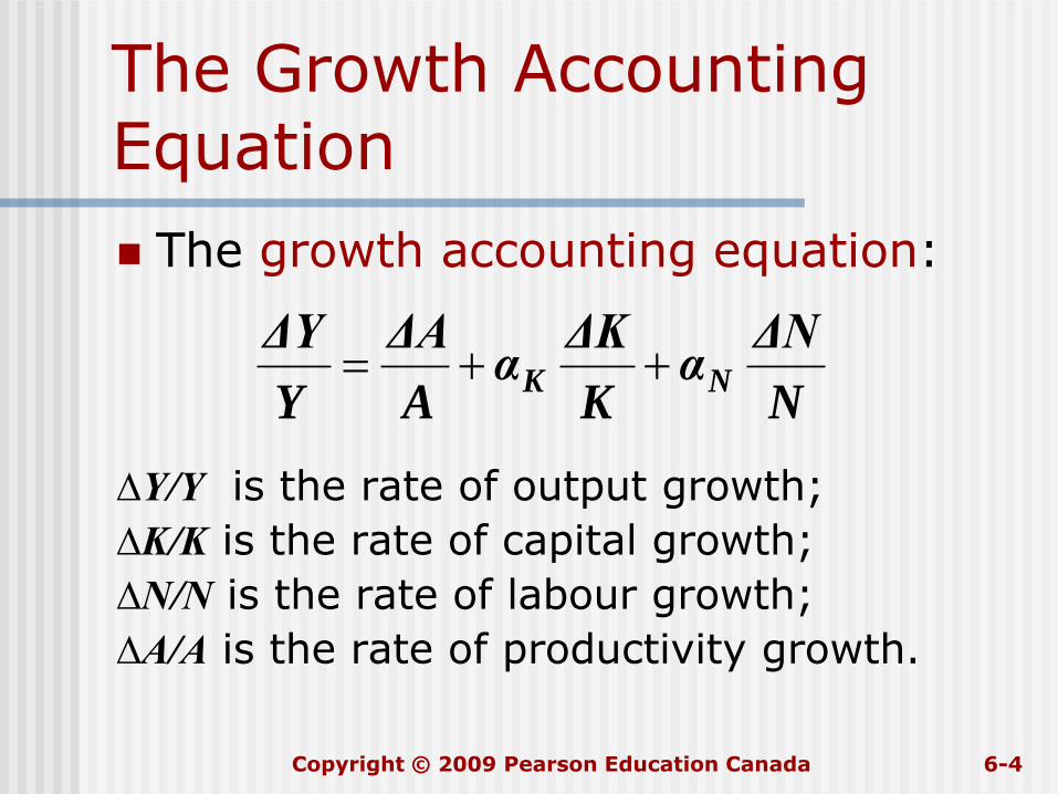
The Growth Accounting Equation

The growth accounting equation:

∆Y/Y is the rate of output growth;

∆K/K is the rate of capital growth;

∆N/N is the rate of labour growth;

∆A/A is the rate of productivity growth.

N

ΔNα

K

ΔKα

A

ΔA

Y

ΔYNK


The Growth Accounting Equation (continued)

= elasticity of output with respect to

capital (about 0.3 in Canada);

= elasticity of output with respect to

labour (about 0.7 in Canada).

The elasticity of output with respect to capital/labour is the percentage increase in output resulting from a one per cent increase in the amount of capital stock/labour.

Kα

Nα

The Growth Accounting Equation (continued) There is another way to derive the equation

using logs. The production function can be written as:

ln(Y) = ln(A) + αKln(K) + αLln(N)

The term “ln” means the natural log of the

variable in question. Since the first derivative of the log of a variable is approximately equal to the proportional change then:

dln(Y) = dln(A) + αKdln(K) + αLdln(N)

This is approximately equal to growth accounting equation in slide 4.



Growth Accounting Growth accounting measures empirically the

relative importance of capital stock, labour and productivity for economic growth.

The impact of changes in capital and labour is estimated from historical data.

The impact of changes in total factor productivity is treated as a residual, that is, not otherwise explained.

N

ΔNα

K

ΔKα

Y

ΔY

A

ΔANK


Growth Accounting and the Productivity Slowdown

Rapid output growth during 1962-1973 has slowed in 1974-2006.

Much of the decline in output growth can be accounted for by a decline in productivity growth.

The slowdown in productivity starting in 1974 was widespread, suggesting a global phenomenon.


The Post-1973 Slowdown in Productivity Growth

Explanations of the reduced growth in productivity are:

Output measurement problem:

• Quality of output and inputs

• Shifts to lower productivity sectors

• Measurement problems have always been there

Technological depletion and slow commercial adaptation:

• The easy stuff has been used up

• Firms slow to take up new technologies

The Post-1973 Slowdown in Productivity Growth (cont’d)

The dramatic rise in oil prices:• Old capital was energy inefficient

• Timing and the fact that the slowdown was international in scope make this an attractive story

• But price of capital did not fall and energy was not that important for several sectors

• As well, productivity should have picked up when oil prices fell in the 1980s – it didn’t

The beginning of new industrial revolution:• The beginning of the computer age

• Takes time to adopt new technologies

• Have seen some pick up in productivity

• The industrial revolution was like thisCopyright © 2009 Pearson Education Canada 6-12


Growth Dynamics: The Neoclassical Growth Model

Accounting approach is just that – it is not an explanation of growth.

The neoclassical growth model:

clarifies how capital accumulation and economic growth are interrelated;

explains the factors affecting a nation’s long-run standard of living;

is suggestive of how a nation’s rate of economic growth evolves over time; and

can say something about convergence – do poor countries/regions catch up?


Assumptions of The Model of Economic Growth

Assume that:

population (Nt) is growing;

at any point in time the share of the population of working age is fixed;

both the population and workforce grow at a fixed rate n;

the economy is closed and there are no government purchases.


Setup of the Model of Economic Growth

Part of the output produced each year is invested in new capital or in replacing worn-out capital (It).

The part of output not invested is consumed (Ct).

ttt IYC


The per-Worker Production Function

The production function in per worker terms is:

(6.5)

yt=Yt/Nt is output per worker in year t

kt=Kt/Nt is capital stock per worker in year t

At= the level of total factor productivity in year t

When the production is written like (6.5) it is often called the intensive form.

)f(kAy ttt


Graph of the per-Worker Production Function

The production function slopes upward. As we move rightward, K is rising faster than N so that k increases.

With more capital, each worker can produce more output.

The slope gets flatter at higher levels of capital per worker. This reflects diminishing MPK.

Output per Worker as a Function of Capital per Worker



Steady States

In a growth model, equilibrium is defined by something called the steady state.

A steady state is a situation in which the economy’s output per worker (yt), consumption per worker (ct), and capital stock per worker (kt) are constant; they

do not change over time.

Remember that these variables are all ratios to Nt so that for example both Yand N are growing.


Steady States (continued)

In the absence of productivity growth the economy reaches a steady state in the long run.

Since yt, ct and kt are constant in a steady-state, Yt, Ct and Kt all grow at rate n, the rate of growth of the

workforce.

As noted above, this is the definition of the steady state.


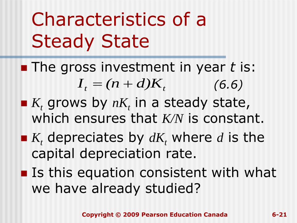
Characteristics of aSteady State

The gross investment in year t is:

(6.6)

Kt grows by nKt in a steady state, which ensures that K/N is constant.

Kt depreciates by dKt where d is the

capital depreciation rate.

Is this equation consistent with what we have already studied?

tt d)K(nI

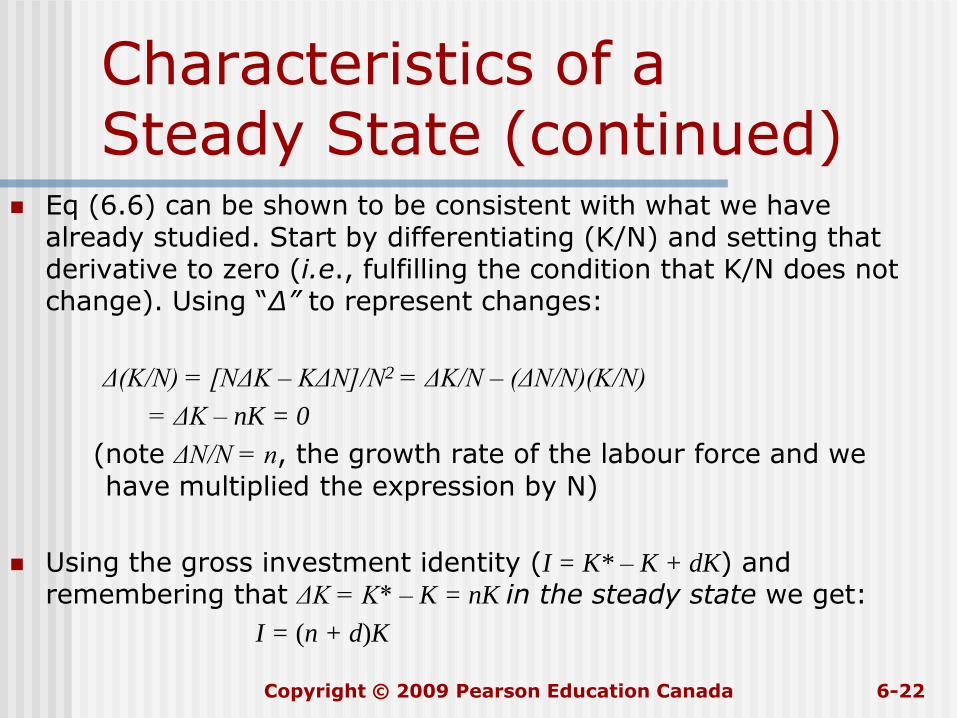
Characteristics of aSteady State (continued)

Eq (6.6) can be shown to be consistent with what we have already studied. Start by differentiating (K/N) and setting that derivative to zero (i.e., fulfilling the condition that K/N does not change). Using “Δ” to represent changes:

Δ(K/N) = [NΔK – KΔN]/N2 = ΔK/N – (ΔN/N)(K/N)

= ΔK – nK = 0

(note ΔN/N = n, the growth rate of the labour force and we

have multiplied the expression by N)

Using the gross investment identity (I = K* – K + dK) and remembering that ΔK = K* – K = nK in the steady state we get:

I = (n + d)K



Characteristics of aSteady State (continued)

Consumption is total output less the amount used for investment.

(6.7)

Put Eq. (6.7) in per-worker terms.

Replace yt with Atf(kt) (Eq. (6.5)).

(6.8)d)kAf(k)-(nc

ttt d)K(n-YC


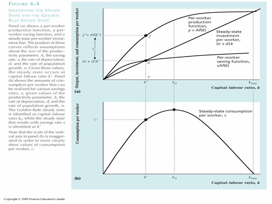
Steady-State Consumption per Worker

An increase in the steady-state capital-labour ratio has two opposing effects on consumption per worker:

1) it raises the amount of output a worker can produce, Af(k); and

2) it increases the amount of output per worker that must be devoted toinvestment, (n + d)k.


Steady-State Consumption per Worker (continued)

The Golden Rule level of the capital stock maximizes consumption per worker in the steady state.

At that point the slope of the production function (it’s derivative wrt to k) equals (n + d),

the slope of the investment line.

From this we can show that r = n, sometimes

referred to as the biological interest rate. The key here is to use the definition of the user cost of capital assuming no taxes and a price of capital equal to one.


Steady-State Consumption per Worker (continued)

The model shows that economic policy focused solely on increasing capital per worker may do little to increase consumption possibilities of the country citizens, if we are close to the Golden Rule level of k.

Empirical evidence is that, given existing starting conditions, a higher capital stock would not lead to less consumption in the long run; i.e., economies are far away from kG.

We will assume that an increase in the steady-state capital-labour ratio raises steady-state consumption per worker.


Reaching the Steady State

We haven’t described how an economy would a steady state.

Why will the described economy reach a steady state?

Which steady state will the economy reach?


Reaching the Steady State(continued)

The piece of information we need is saving.

Assume that saving in this economy is proportional to current income:

(6.9)

“s” is a number between 0 and 1. It

represents the faction of current income saved.

tt sYS



National saving (in this case, private saving as there is no government in the model) has to equal investment.

Here we we set our simple saving function equal to investment:

(6.10)tt d)K(nsY



Put Eq. (6.10) in per-worker terms.

Replace Yt with Atf(kt) (Eq. (6.5))

(6.11)

Subscript t is dropped because the variables are constant in the steady state.

d)k(nsAf(k)


Steady-State Capital-Output Ratio

Equation 6.11 says that the steady state capital-labour ratio must ensure that saving per worker and investment per worker are equal.

k* is the value of k at which the saving

curve and the steady-state investment line cross.

k* is the only possible steady-state

capital-output ratio for this economy.


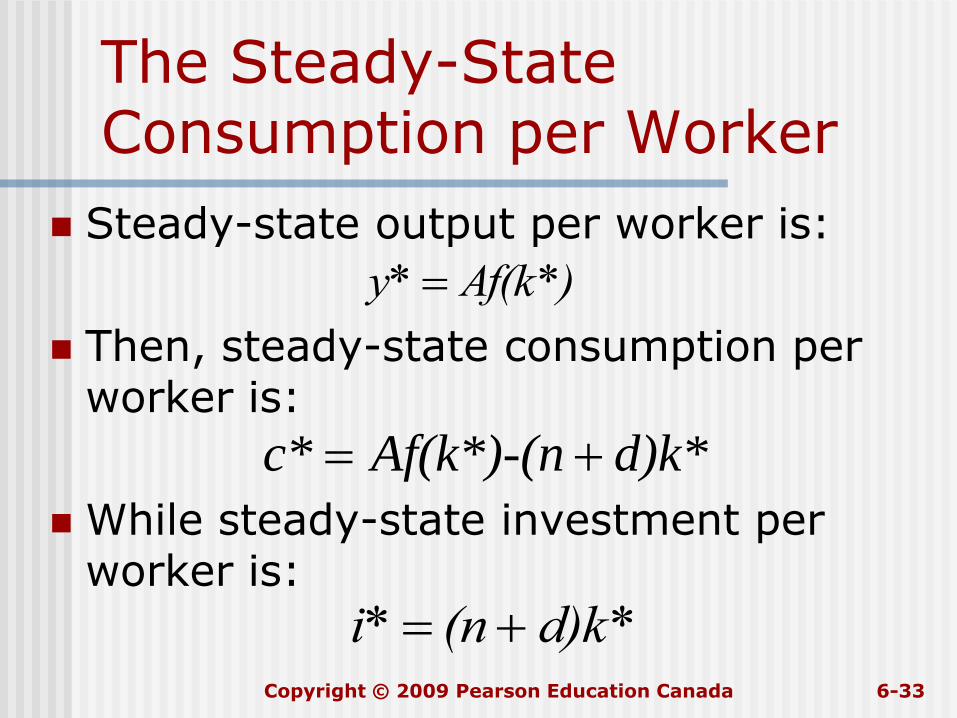
The Steady-State Consumption per Worker

Steady-state output per worker is:

Then, steady-state consumption per worker is:

While steady-state investment per worker is:

d)k*Af(k*)-(nc*

y* Af(k*)

i* (n d)k*


The Model Implications

The economy’s capital-labour ratio has a tendency to go to k*. It will remain there forever, unless something changes.

In this steady state the capital-labour ratio, output per worker, investment per worker, and consumption per worker all remain constant over time.

The model determines an equilibrium but not growth – that is given by assumption.

The Model Implications (continued)

If the level of saving were greater than the amount of investment needed to keep k

constant, then that extra saving gets converted into capital and k rises.

If saving were less than the amount needed to keep k constant, the reverse would happen – k would fall.

Note that there is no reason to suppose that the steady state is at a point of maximum consumption – the “Golden Rule”.



The Determinants of Long-Run Living Standard

Long-run well-being is measured here by the steady-state level of consumption per worker.

Its determinants are:

1) the saving rate (s);

2) the population growth rate (n);

3) the rate of productivity growth (how fast A grows).


Long-Run Living Standard and the Saving Rate

A higher saving rate implies a higher living standard. The increased saving rate raises output at every level of capital per worker.

A steady-state with higher output and consumption per worker is attained in the long run.


The Saving Rate (continued)

An increase in the saving rate has a cost – a fall in current period consumption.

As before in the decision to consume, there is a trade-off between current current and future consumption.

Beyond a certain point the cost of lost consumption today will outweigh the future benefits.

The Saving Rate (continued)

It is also the case that a policy that increases saving will generate a temporary spurt in the growth rate.

Since y = Y/N and N is growing at a constant rate (n), then as we move to a new and higher k* output must grow faster than n at least temporarily.


Effect of an Increase in Saving Rate



Long-Run Living Standard and Population Growth

Increased population growth tends to lower living standards.

When the workforce is growing rapidly, a larger part of current output must be devoted to just providing capital for the new workers to use.

Absent here is any effect increased population may have on output –increased immigration of highly skilled workers would improve growth.


Population Growth (continued)

However, a reduction in population growth means:

lower population and lower total productive capacity;

lower ratio of working-age people to the population and perhaps an unsustainable pension system.

In some countries, low population growth can be raised by encouraging immigration and higher female participation.

Effects of Higher Population Growth



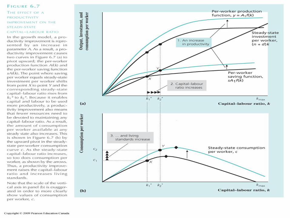
Long-Run Living Standard and Productivity Growth

The model accounts for the sustained growthby incorporating productivity growth.

Increased productivity will improve living standards:

it raises y at every k;

then saving per worker increases;

and higher k* is attained.

This is important. Without productivity improvements, living standards would remain unchanged.


Productivity Growth (continued)

A one-time productivity improvement shifts the economy only from one steady state to a higher one.

Only continuing increases in productivity can perpetually improve living standards.

Remember again, productivity growth is exogenous in this model.

An Improvement in Productivity



Do Economies Converge? Unconditional convergence is a situation when the

poor countries eventually catch up to the rich countries so that in the long run, living standards around the world become more or less the same.

Certain conditions apply. For example, if the only difference is K/N but all else is the same (s, n, A)

then the model predicts that living standards will converge.

Some evidence suggests yes – poorer countries have tended to grow faster than richer ones.

Trade and capital flows may be routes that facilitate unconditional convergence (Fischer’s results).


Do Economies Converge?(continued)

Conditional convergence is a situation when living standards will converge only within a group of countries with similar characteristics.

OECD and developing economies could be considered two such groups.

This result occurs if there are differences in s, n and A.

Do Economies Converge?(continued)

Most findings find support for the idea of conditional convergence.

Studies show that low saving (including human capital) in developing countries are important in explaining growth differences.

Capital flows are again important.

Other studies highlight importance of competition as well as the functioning of labour markets and macroeconomic policy.



Implication of the Neoclassical Growth Theory

The neoclassical model highlights the role and importance of productivity

However, it assumes, rather than explains, productivity – the crucial determinant of living standards (see first part of chapter).

In other words, the model does not explain growth in output per capitawhich is what is of great interest.


Endogenous Growth Theory

Endogenous growth theory tries to explain productivity growth within the model (endogenously).

An implication of endogenous growth theory is that a country’s growth rate depends on its rate of saving and investment, not only on exogenous productivity growth.


Setup of the Endogenous Growth Model

Assume that the number of workers remains constant.

This implies that the growth rate of output per worker is simply equal to the growth rate of output.

The aggregate production function is:

(6.11)

Where A is a positive constant.

AKY


Setup of the Endogenous Growth Model (continued)

The marginal product of capital (MPK) is equal to A and does not depend on the capital stock (K).

The MPK is not diminishing, it is constant. This is a major departure from the previous growth model.


Constant MPK andHuman Capital

One explanation of constant MPK is human capital – the knowledge, skills, and training of individuals.

As an economy’s physical capital increases its human capital stock tends to increase in the same proportion.

Workers get better at using capital –there is learning-by-doing – an idea due to Arrow.


Constant MPK andResearch and Development

Another explanation of constant MPK is research and development (R&D) activities.

The resulting productivity gains offset any tendency for the MPK to decrease.

As the economy grows, firms have an incentive to invest in R&D.


The Model of Endogenous Growth

Assume that national saving, S, is a constant fraction s of aggregate output, AK, so that S = sAK.

In a closed economy I=S.

As we know, total gross investment equals net investment plus depreciation

I = ∆K + dK


The Model of Endogenous Growth (continued)

Therefore: (6.13)

(6.14)

(6.15)

Since the growth rate of output is proportional to the growth rate of capital stock.

dsAY

ΔYand

dsAK

ΔK or

sAKdKΔK


Implication of The Model of Endogenous Growth The endogenous growth model places greater

emphasis on saving, human capital formation and R&D as sources of long-run growth.

Higher saving and capital formation generate investment in human capital and R&D raising A.

Remember, in the neoclassical (or Solow-Swan) growth model, the saving rate affects only the level of output, not growth.

One problem is that it can be difficult to distinguish this model from conditional convergence.


Economic Growth and the Environment

So far we have assumed that there are no natural limits to growth, like declining non-renewable resources or the environment.

The empirical facts:

Levels of many pollutants rise and then fall as economy grows.

The costs of controlling pollution are rising but remain relatively constant as a fraction of GDP.

Pollution emissions per unit of GDP have been falling since the late 1940s.


Economic Growth and the Environment (continued)

During the rapid initial economic growth phase the impact of output growth overwhelms the improvements in pollution-abatement technology.

Near the steady state economic growth slows down and technological progress in pollution control overwhelms the impact of economic growth.

These results are often due to policy choices.


Government Policies and Long-Run Living Standards

Government policies that are useful in raising a country’s long-run standard of living are:

polices to raise the saving rate;

policies to raise the rate of productivity.


Policies to Affect theSaving Rate

By taxing consumption a government can exempt from taxation the income that is saved.

A government can increase the amount that it saves by reducing its deficit.


Affecting productivity Growth: Improving Infrastructure

Some research finds a link between productivity and the quality of nation’s infrastructure.

Other research finds that public investments cannot explain cross-country differences.

Higher growth in productivity may lead to more infrastructure, and not vice versa; that is, richer countries may want better infrastructure, like roads, schools and hospitals.


Affecting productivity Growth: Building Human Capital Recent research finds a strong

connection between productivity growth and human capital.

Governments affect human capital through education policies, training programs, health programs, etc.

Productivity growth may increase if barriers to entrepreneurial activity are removed and competition increased.


Affecting productivity Growth: Research and Development

Direct government support of basic research is a good investment for raising productivity.

Some economists believe that even commercially-oriented research deserves government aid.

Here public-private partnerships may help.


Affecting productivity Growth: Industrial Policy

Industrial policy is a growth strategy in which the government attempts to influence the country’s pattern of industrial development.

The arguments for the industrial policy are borrowing constraints, spillovers, and nationalism. The danger is favouritism.

“Government’s are not very good at finding winners, but losers are good at finding governments.” Sylvia Ostry


Affecting productivity Growth: Market Policy

Market policy is government restriction on free markets.

Economists favour respect for property rights and a reliance on free markets to allocate resources efficiently.

The reasons for government to interfere are market failures and efficiency vs. equity trade-off.

Solving the Model for Key Variables

We can use the neo-classical growth model to solve for various key variables.

To determine the steady-state capital-labour ratio (k*), start with the equilibrium condition that S=I in per capita terms.

Thus:

(n+d)k* = sAk*α

This implies that k* is:

k* = [sA/(n+d)]1/(1-α)


Solving the Model for Key Variables (continued)

Suppose we want to know the Golden Rule level of the capital-labour ratio, kG.

From Figure 6.2, when the marginal productivity of k equal n + d, we

know that consumption is maximised and the capital-labour ratio = kG.



Assuming that the production function, in intensive form, is Cobb-Douglas (y = Akα), then the marginal product of k is αAkα-1. Substituting in kG into this relationship and setting it equal to n + d, we get:

αAkGα-1 = n + d

It then follows that:

kG = [(αA)/(n+d)]1/(1-α)

We can now solve for y, investment and c.



If we wanted to know what saving rate (s) would get us to kG, (whose value we now know) we go back to our

old friend saving = investment and assume that we were at the point kG.

sAkGα = (n + d)kG

Then s is given by:

s = [(n + d)/A]kG1-α

The strategy is to go to the point kG and ask the question: what

must have been s to get us to this point.

Once we know kG we can solve for y and investment, which of course gives us c.



Using the saving = investment identity we can solve for the effects of other changes.

Suppose we want to know what is the effect of higher labour for growth (n’). From the S/I identity

we have:

sAkα = (n’ + d)k

Which yields a new k equal to:

kn’ = [sA/(n’ + d)]1/(1–α)

We can use kn’ (the capital/labour ratio resulting from n’) to calculate the new y, investment and c.



A productivity improvement (call it A’) can be

handled in a similar fashion; i.e., through the saving-investment identity.

sA’kα = (n + d)k

Then as before, we solve for a new k,

kA’ = [sA’/(n + d)]1/(1–α)

Once we have kA’ we proceed as before and

get the other variables of interest.

Remember, when re-calculating y, adjust it for

the now larger productivity, A’.Copyright © 2009 Pearson Education Canada

6-75

Solving the Model for Key Variables in Discrete Time Start with the following

Kt+1 – Kt = It – dKt, which is the capital

accumulation identity and can be written as:

Kt+1 = (1 – d)Kt + It

The labour force (or population) evolves as:

Nt+1 = (1 + n)Nt, where n is the growth rate of

labour.

Divide both sides by Nt+1 bearing in mind the growth of labour equation and that St = It:

Kt+1/Nt+1 – Kt/(1+n)Nt = sAKtα/(1+n)Nt – dKt/(1+n)Nt


Solving the Model for Key Variables in Discrete Time (con’t)

Remembering that k = K/N, the equation on the

previous slide can be written as:

kt+1 = (1-d)/(1+n)kt + [s/(1+n)]Aktα

This expression shows what is called the law of motion of capital. Simply stated, it shows how the capital stock per worker (kt+1) evolves over time.

As can be seen, kt+1 depends on the amount of capital already in place – kt, times (1-d)/(1+n) – as well as the amount of new capital being added – [s(1+n)]Akt

α, divided by (1+n).

Next we show that the implied steady state capital labour ratio is the same as derived in slide 70.


Solving the Model for Key Variables in Discrete Time (con’t)

Multiplying both sides by 1+n we get:

(1+n) kt+1 – (1–d) kt = sAktα

In the steady kt+1 = kt = k the equation

becomes:

(n+d)k = sAkα

The steady state level of capital per worker (k*) is then:

k* = [sA/(n+d)]1/(1-α)

This is identical to the expression in slide 70.


chapter 6 -...

Documents