chapter 6 the normal probability distribution general objectives: you will learn about continuous...

Chapter 6 The Normal Probability Distribution

General Objectives:

You will learn about continuous random variables and their probability distributions. You will learn how to calculate normal probabilities and, under certain conditions, how to use the normal probability distribution to approximate the binomial probability distribution.

©1998 Brooks/Cole Publishing/ITP

Specific Topics

1. Probability distributions for continuous random variables

2. The normal probability distribution.

3. Calculation of areas associated with the normal probability distribution

4. The normal approximation


6.1 Probability Distributions for Continuous Random Variables

Continuous random variables can assume the infinitely many values corresponding to points on a line interval.

Examples: Heights, weights, length of life of a particular product, experimental laboratory error

A smooth curve describes the probability distribution of a continuous random variable.

The depth or density of the probability, which varies with x, may be described by a mathematical formula f (x ), called the distribution for the random variable x.


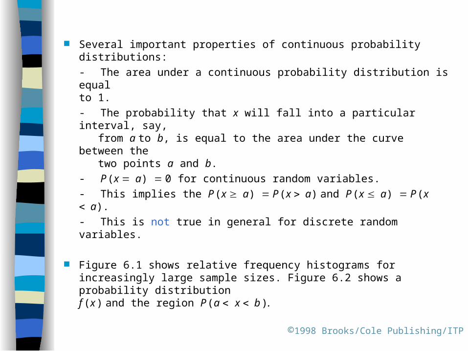
Several important properties of continuous probability distributions:

- The area under a continuous probability distribution is equal

to 1.

- The probability that x will fall into a particular interval, say, from a to b, is equal to the area under the curve between the two points a and b.

- P (x a) 0 for continuous random variables.

- This implies the P (x a) P (x a) and P (x a) P (x a).

- This is not true in general for discrete random variables.

Figure 6.1 shows relative frequency histograms for increasingly large sample sizes. Figure 6.2 shows a probability distribution f (x ) and the region P (a x b ).


Choosing the probability distribution f (x ) appropriate for a given experiment:

- It fits the accumulated body of data.- It allows us to make the best possible inferences using the data.

The normal probability distribution provides a good model for describing data that have mound-shaped frequency distributions.

The Normal Probability Distribution:

where e 2.718 and 3.142; and ( 0 ) are the parameters that represent the population mean and standard deviation.

Figure 6.3 shows the normal probability distribution.


22 2/

21

)(

xexf

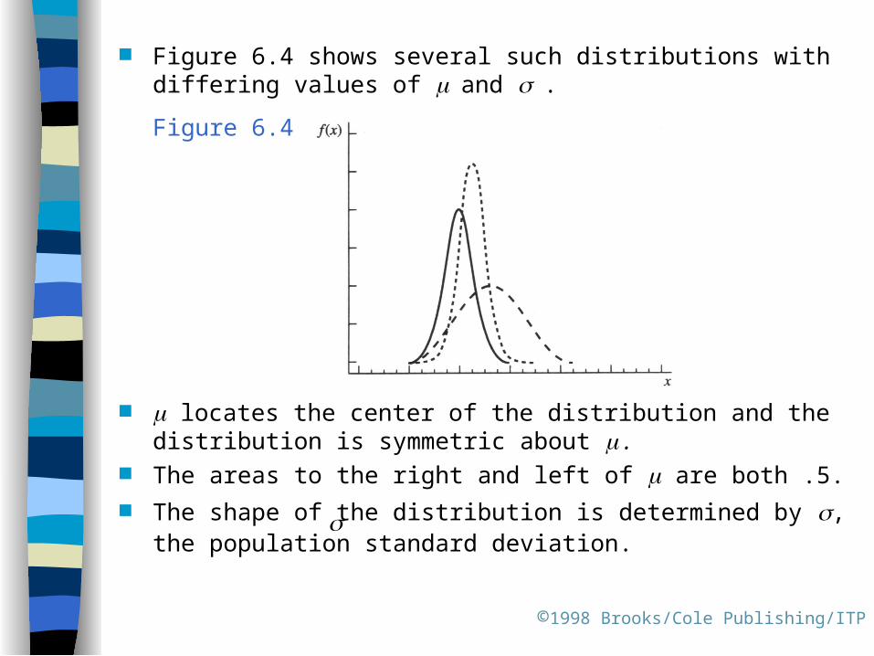
Figure 6.4 shows several such distributions with differing values of and .

Figure 6.4

locates the center of the distribution and the distribution is symmetric about .

The areas to the right and left of are both .5. The shape of the distribution is determined by , the population

standard deviation.


Large values of reduce the height of the curve and increase the spread.

Small values of increase the height of the curve and reduce the spread.

Many positive random variables, such as height, weight, and time, have distributions that are well approximated by a normal distribution.


6.3 Tabulated Areas of the Normal Probability Distributions The probability that a continuous random variable x assumes a

value in the interval a to b is the area under the probability density function between the points a and b.

We use a standardization procedure that allows us to use the same tables of probabilities for all normal distributions.

The Standard Normal Random Variable:

A normal random variable is standardized by expressing its value as the number of standard deviations () it lies to the left or right of its mean . The standardized normal random variable z, is defined as z (x )/ , or equivalently, x z .


From the formula for z, we can draw these conclusions:

- When x is less that the mean , the value of z is negative.

- When x is greater that the mean , the value of z is positive.

- When x , the value z 0. The standard probability distribution has a mean of zero and a

standard deviation of 1. The area under the standard normal curve between mean z 0

and a specified positive value of z, say, z0, is the probability

P(0 z z0). This area is recorded in a table where z, correct to the nearest

tenth, is recorded in the left-hand column of the table, and the second decimal place for z, corresponding to hundredths, is given across the top row.


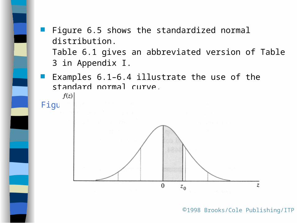
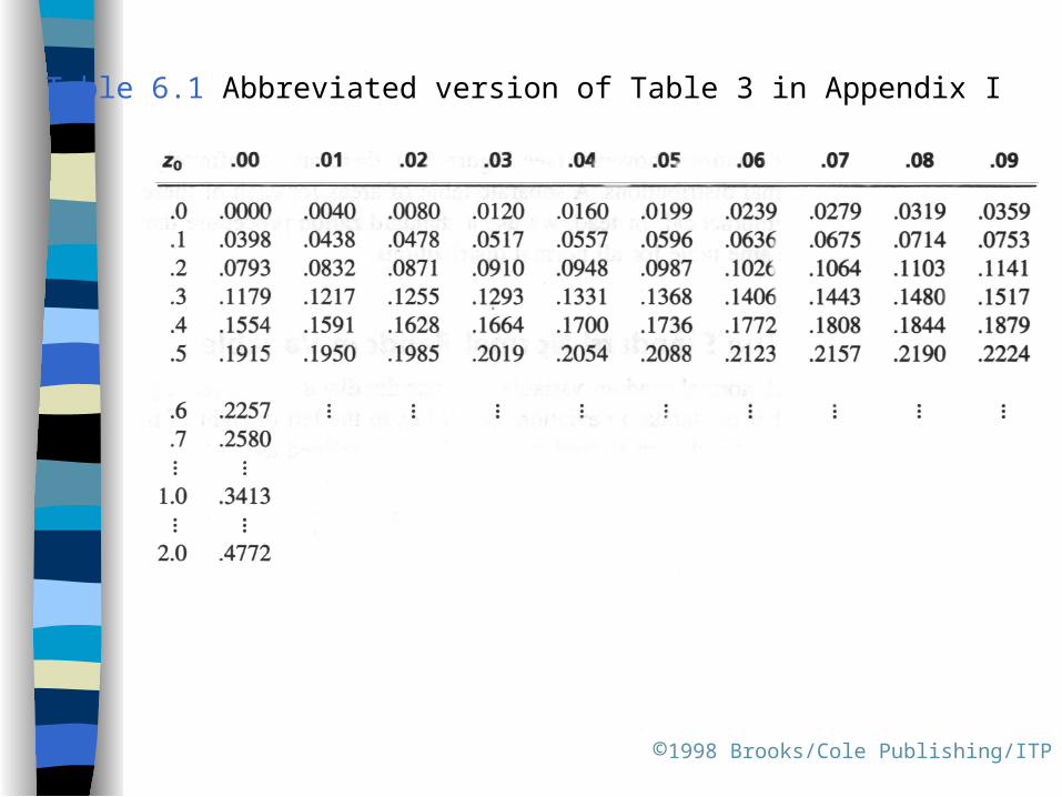
Figure 6.5 shows the standardized normal distribution. Table 6.1 gives an abbreviated version of Table 3 in Appendix I.

Examples 6.1–6.4 illustrate the use of the standard normal curve.

Figure 6.5



Table 6.1 Abbreviated version of Table 3 in Appendix I


Example 6.1

Find P (0 z 1.63). This probability corresponds to the area between the mean (z 0) and a point z 1.63 standard deviations to the right of the mean (see Figure 6.6).

Solution

The area is shaded in Figure 6.6. Since Table 3 in Appendix I gives areas under the normal curve to the right of the mean, you need only find the tabulated value corresponding to z 1.63. Proceed down the left-hand column of the table to z 1.6 and across the top of the table to the column marked .03. The intersection of this row and column combination gives the area A .4484. Therefore, P (0 z 1.63) .4484.


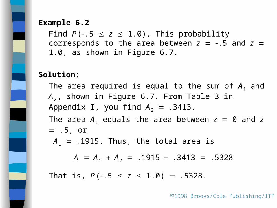
Example 6.2

Find P (.5 z 1.0). This probability corresponds to the area between z .5 and z 1.0, as shown in Figure 6.7.

Solution:

The area required is equal to the sum of A 1 and A 2 , shown in Figure 6.7. From Table 3 in Appendix I, you find A 2 .3413.

The area A 1 equals the area between z 0 and z .5, or

A 1 .1915. Thus, the total area is

A A 1 A 2 .1915.3413 .5328

That is, P (.5 z 1.0) .5328.

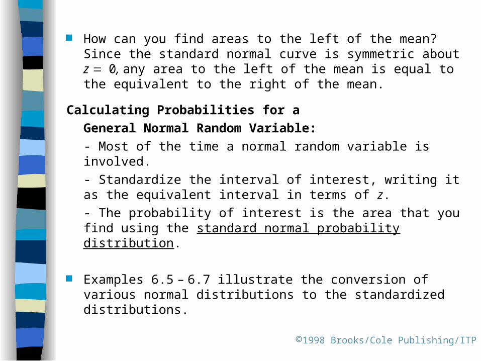
How can you find areas to the left of the mean? Since the standard normal curve is symmetric about z 0, any area to the left of the mean is equal to the equivalent to the right of the mean.

Calculating Probabilities for a

General Normal Random Variable:

- Most of the time a normal random variable is involved.

- Standardize the interval of interest, writing it as the equivalent interval in terms of z.

- The probability of interest is the area that you find using the standard normal probability distribution.

Examples 6.5 – 6.7 illustrate the conversion of various normal distributions to the standardized distributions.


6.4 The Normal Approximation to the Binomial Probability

Distribution (Optional)

Two ways to calculate probabilities for the binomial random variable x:

- Using the binomial formula,

- Using the cumulative binomial tables There is one other option when np 7; the Poisson

probabilities can be used to approximate P(x k). When this does not work and n is large, the normal probability

distribution provides another approximation for binomial probabilities.


knknk qpCkxP )(

The Normal Approximation to the Binomial Probability Distribution:

- Let x be a binomial random variable with n trials and probability p of success.

- The probability distribution of x is approximated using a normal curve with np and .

- This approximation is adequate as long as n is large and p is not too close to 0 or 1.

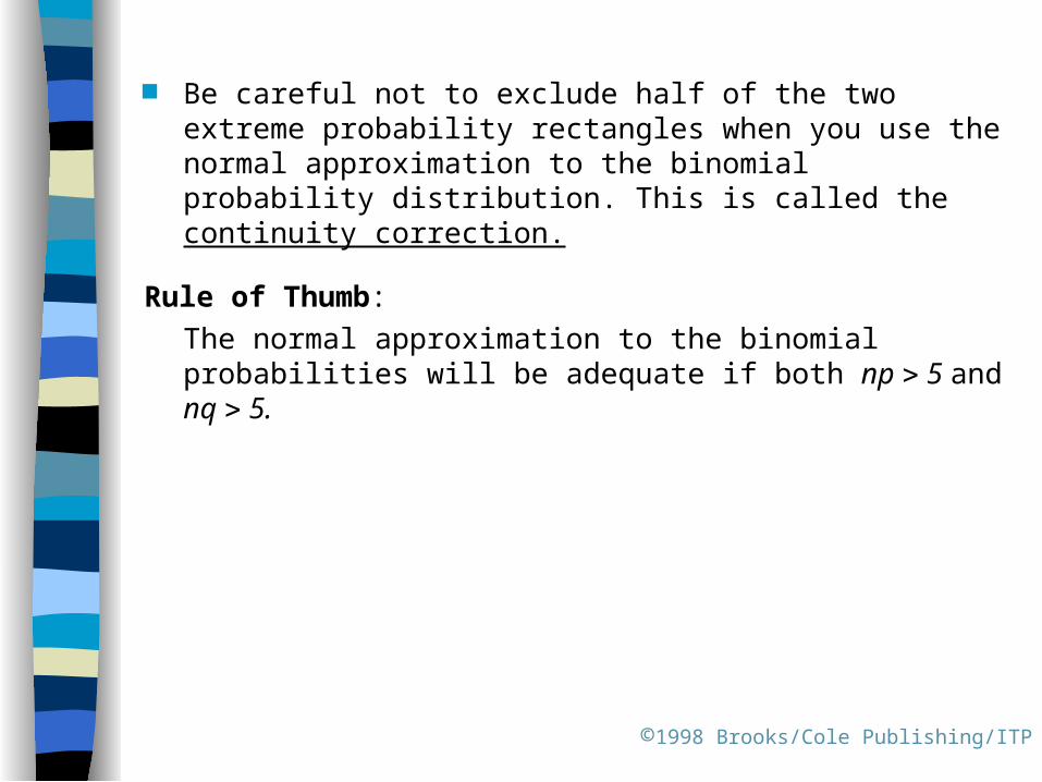
You must be careful not to exclude half of the two extreme probability rectangles when you use the approximation.

This adjustment, called the continuity correction, helps account for the fact that you are approximating a discrete random variable with a continuous one.

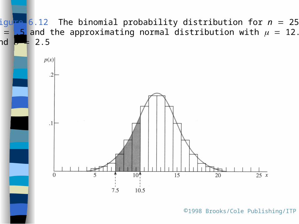
Figure 6.12 shows the binomial probability distribution for n 25 and p .5 and the approximating normal distribution with 12.5 and 2.5. Figure 6.13 shows the binomial probability distribution for n 25 and p .1.


npq

Example 6.8 uses the normal curve to approximate binomial probabilities.

Example 6.8

Use the normal curve to approximate the probability that x 8, 9, or 10 for a binomial random variable with n 25 and p .5. Compare this approximation to the exact binomial probability.

Solution

You can find the exact binomial probability for this example because there are cumulative binomial tables for n 25. From Table 1 in Appendix I,

To use the normal approximation, first find the appropriate mean and standard deviation for the normal curve:


190.022.212.)7()10()10 or ,9 ,8( xPxPxP

5.12)5(.25 np

5.225.6)5)(.5(.25 npq

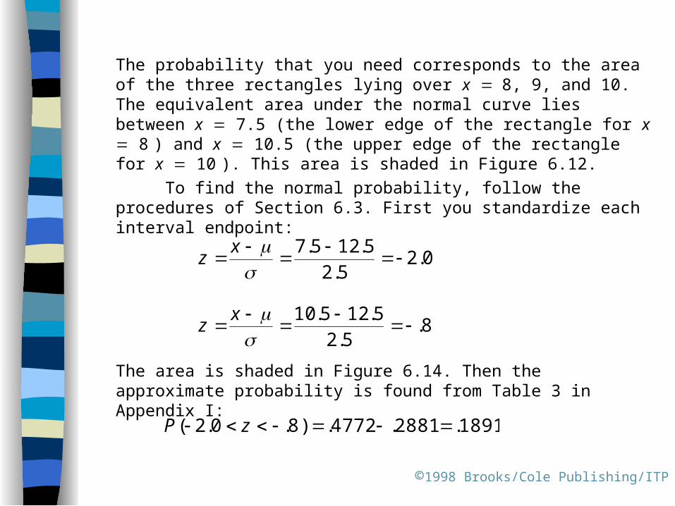
The probability that you need corresponds to the area of the three rectangles lying over x 8, 9, and 10. The equivalent area under the normal curve lies between x 7.5 (the lower edge of the rectangle for x 8 ) and x 10.5 (the upper edge of the rectangle for x 10 ). This area is shaded in Figure 6.12.

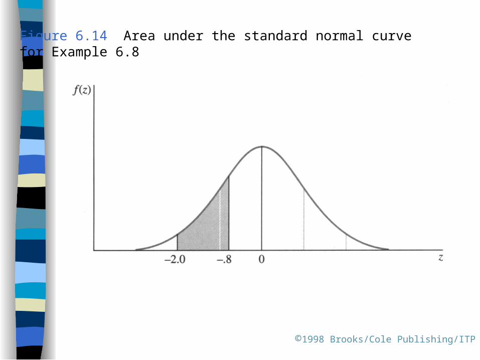
To find the normal probability, follow the procedures of Section 6.3. First you standardize each interval endpoint:

The area is shaded in Figure 6.14. Then the approximate probability is found from Table 3 in Appendix I:


0.25.2

5.125.7

xz

8.5.2

5.125.10

xz

1891.2881.4772.)8.0.2( zP


Figure 6.12 The binomial probability distribution for n 25 and p .5 and the approximating normal distribution with 12.5 and 2.5


Figure 6.14 Area under the standard normal curve for Example 6.8


Be careful not to exclude half of the two extreme probability rectangles when you use the normal approximation to the binomial probability distribution. This is called the continuity correction.

Rule of Thumb:

The normal approximation to the binomial probabilities will be adequate if both np 5 and nq 5.

©1998 Brooks/Cole Publishing/ITP-

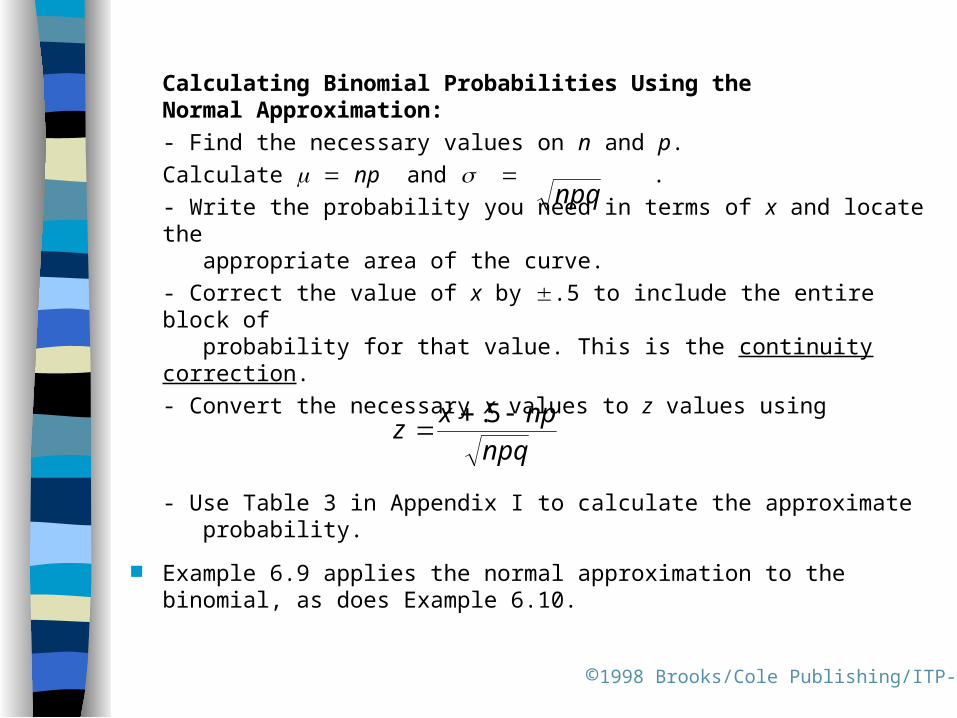
Calculating Binomial Probabilities Using the Normal Approximation:

- Find the necessary values on n and p.

Calculate np and .

- Write the probability you need in terms of x and locate the appropriate area of the curve.

- Correct the value of x by .5 to include the entire block of probability for that value. This is the continuity correction.

- Convert the necessary x values to z values using

- Use Table 3 in Appendix I to calculate the approximate probability.

Example 6.9 applies the normal approximation to the binomial, as does Example 6.10.

npq

npxz

5.

npq


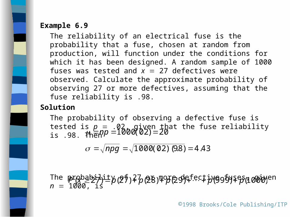
Example 6.9

The reliability of an electrical fuse is the probability that a fuse, chosen at random from production, will function under the conditions for which it has been designed. A random sample of 1000 fuses was tested and x 27 defectives were observed. Calculate the approximate probability of observing 27 or more defectives, assuming that the fuse reliability is .98.

Solution

The probability of observing a defective fuse is tested is p .02, given that the fuse reliability is .98. Then

The probability of 27 or more defective fuses, given n 1000, is

20)02(.1000 np

43.4)98)(.02(.1000 npg

)1000()999()29()28()27()27( pppppxP


It is appropriate to use the normal approximation to the binomial probability because

np 1000(.02) 20 and nq 1000(.98) 980

are both greater than 5. The normal area used to approximate P (x 27) is the are under the normal curve to the right of 26.5, so that the entire rectangle for x 27 is included. Then, the z-value corresponding to x 26.5 is

and the area between z 0 and z 21.47 is equal to .4292, as shown in Figure 6.15. Since the total area to the right of the mean is equal to .5, you have

P (x 27) P (z 1.47) .5 .4292 .0708

47.143.45.6

43.4205.26

x

z


Key Concepts and Formulas

I. Continuous Probability Distributions

1. Continuous random variables

2. Probability distributions or probability density functions

a. Curves are smooth.

b. The area under the curve between a and b represents the probability that x falls between a and b.

C. P (X a) 0 for continuous random variables.

II. The Normal Probability Distribution

1. Symmetric about its mean .

2. Shape determined by its standard deviation .


III. The Standard Normal Distribution

1. The normal random variable z has mean 0 and standard deviation 1.

2. Any normal random variable x can be transformed to a standard normal random variable using

3. Convert necessary values of x to z.

4. Use Table 3 in Appendix I to compute standard normal probabilities.

5. Several important z-values have tail areas as follows:

Tail Area: .005 .01 .025 .05 .10

z-Value: 2.58 2.33 1.96 1.645 1.28

x

z

chapter 6 the normal probability distribution general objectives: you will learn about continuous...

Documents