chapter 6d. numerical interpolation finite difference interpolation
TRANSCRIPT
1
� A. J. Clark School of Engineering �Department of Civil and Environmental Engineering
by
Dr. Ibrahim A. AssakkafSpring 2001
ENCE 203 - Computation Methods in Civil Engineering IIDepartment of Civil and Environmental Engineering
University of Maryland, College Park
CHAPTER 6d.NUMERICAL INTERPOLATION
© Assakkaf
Slide No. 99
� A. J. Clark School of Engineering � Department of Civil and Environmental Engineering
ENCE 203 � CHAPTER 6d. NUMERICAL INTERPOLATION
Finite Difference Interpolation
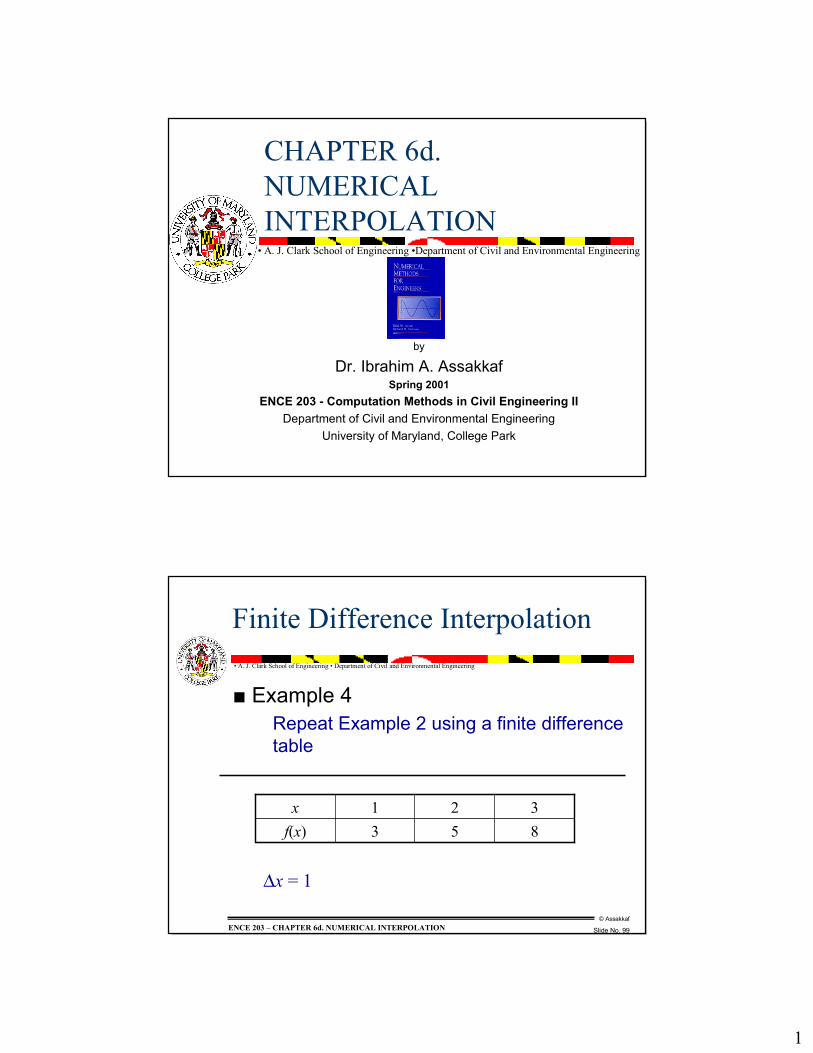
� Example 4Repeat Example 2 using a finite difference table
853f(x)321x
∆x = 1
2
© Assakkaf
Slide No. 100
� A. J. Clark School of Engineering � Department of Civil and Environmental Engineering
ENCE 203 � CHAPTER 6d. NUMERICAL INTERPOLATION
f(x + n∆x)x + n∆x
∆ f [x +( n-1)∆x]∆2 f [x +( n-2)∆x]f [x +( n-1)∆x]x +( n-1)∆x
∆3 f [x +( n-3)∆x]∆ f [x +( n-2)∆x]∆2 f [x +( n-3)∆x]f [x +( n-2)∆x]x +( n-2)∆x
∆nf(x)::::::::∆2 f(x + 3∆x)
∆3 f(x + 2∆x)∆ f(x + 3∆x)∆2 f(x + 2∆x)f(x + 3∆x)x + 3∆x
∆3 f(x + ∆x)∆ f(x + 2∆x)∆2 f(x + ∆x)f(x + 2∆x)x + 2∆x
∆3f(x)∆ f(x + ∆x)∆2f(x)f(x + ∆x)x + ∆x
∆f(x)
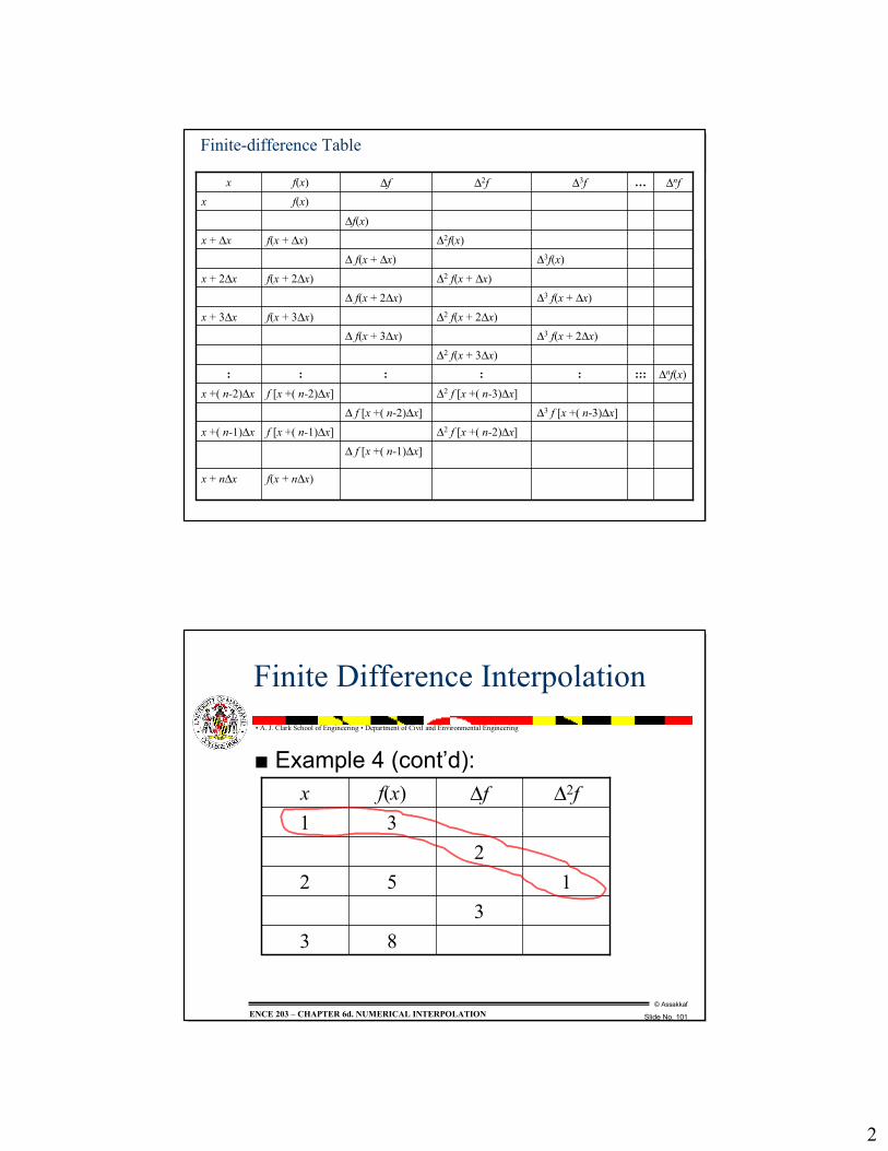
f(x)x∆nf�∆3f∆2f∆ff(x)x
Finite-difference Table
© Assakkaf
Slide No. 101
� A. J. Clark School of Engineering � Department of Civil and Environmental Engineering
ENCE 203 � CHAPTER 6d. NUMERICAL INTERPOLATION
Finite Difference Interpolation
� Example 4 (cont�d):
833
1522
31∆2f∆ff(x)x
3
© Assakkaf
Slide No. 102
� A. J. Clark School of Engineering � Department of Civil and Environmental Engineering
ENCE 203 � CHAPTER 6d. NUMERICAL INTERPOLATION
Finite Difference Interpolation
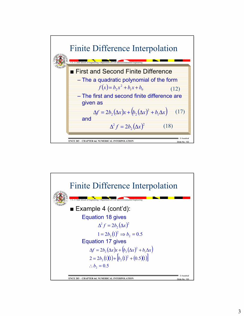
� First and Second Finite Difference� The a quadratic polynomial of the form
� The first and second finite difference are given as
and
( ) 012
2 bxbxbxf ++=
( ) ( )( )xbxbxxbf ∆+∆+∆=∆ 12
222
( )22
2 2 xbf ∆=∆
(17)
(18)
(12)
© Assakkaf
Slide No. 103
� A. J. Clark School of Engineering � Department of Civil and Environmental Engineering
ENCE 203 � CHAPTER 6d. NUMERICAL INTERPOLATION
Finite Difference Interpolation
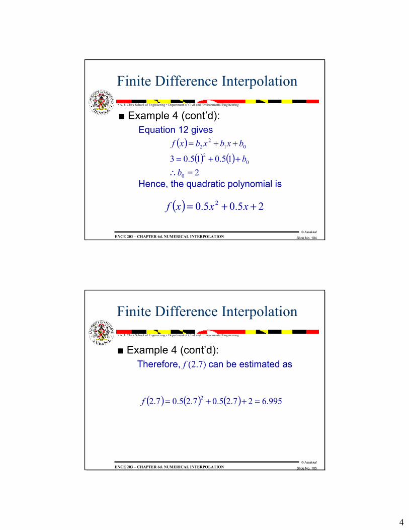
� Example 4 (cont�d):Equation 18 gives
Equation 17 gives
( )( ) 5.0121
2
22
2
22
2
=⇒=
∆=∆
bb
xbf
( ) ( )( )( )( ) ( ) ( )( )[ ]
5.015.011122
2
2
222
12
22
=∴++=
∆+∆+∆=∆
bbb
xbxbxxbf
4
© Assakkaf
Slide No. 104
� A. J. Clark School of Engineering � Department of Civil and Environmental Engineering
ENCE 203 � CHAPTER 6d. NUMERICAL INTERPOLATION
Finite Difference Interpolation
� Example 4 (cont�d):Equation 12 gives
Hence, the quadratic polynomial is
( )( ) ( )2
15.015.03
0
02
012
2
=∴++=
++=
bb
bxbxbxf
( ) 25.05.0 2 ++= xxxf
© Assakkaf
Slide No. 105
� A. J. Clark School of Engineering � Department of Civil and Environmental Engineering
ENCE 203 � CHAPTER 6d. NUMERICAL INTERPOLATION
Finite Difference Interpolation
� Example 4 (cont�d):Therefore, f (2.7) can be estimated as
( ) ( ) ( ) 995.627.25.07.25.07.2 2 =++=f
5
© Assakkaf
Slide No. 106
� A. J. Clark School of Engineering � Department of Civil and Environmental Engineering
ENCE 203 � CHAPTER 6d. NUMERICAL INTERPOLATION
Finite Difference Interpolation
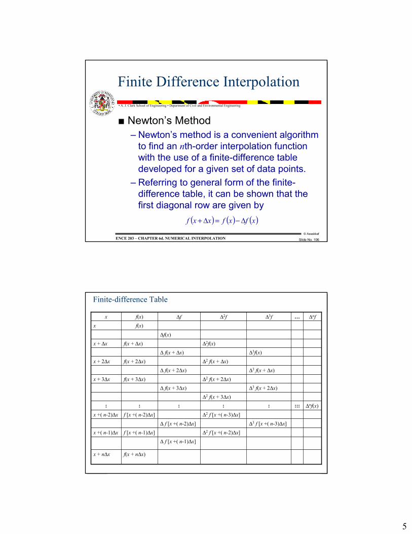
� Newton�s Method� Newton�s method is a convenient algorithm
to find an nth-order interpolation function with the use of a finite-difference table developed for a given set of data points.
� Referring to general form of the finite-difference table, it can be shown that the first diagonal row are given by
( ) ( ) ( )xfxfxxf ∆−=∆+
© Assakkaf
Slide No. 107
� A. J. Clark School of Engineering � Department of Civil and Environmental Engineering
ENCE 203 � CHAPTER 6d. NUMERICAL INTERPOLATION
f(x + n∆x)x + n∆x
∆ f [x +( n-1)∆x]∆2 f [x +( n-2)∆x]f [x +( n-1)∆x]x +( n-1)∆x
∆3 f [x +( n-3)∆x]∆ f [x +( n-2)∆x]∆2 f [x +( n-3)∆x]f [x +( n-2)∆x]x +( n-2)∆x
∆nf(x)::::::::∆2 f(x + 3∆x)
∆3 f(x + 2∆x)∆ f(x + 3∆x)∆2 f(x + 2∆x)f(x + 3∆x)x + 3∆x
∆3 f(x + ∆x)∆ f(x + 2∆x)∆2 f(x + ∆x)f(x + 2∆x)x + 2∆x
∆3f(x)∆ f(x + ∆x)∆2f(x)f(x + ∆x)x + ∆x
∆f(x)
f(x)x∆nf�∆3f∆2f∆ff(x)x
Finite-difference Table
6
© Assakkaf
Slide No. 108
� A. J. Clark School of Engineering � Department of Civil and Environmental Engineering
ENCE 203 � CHAPTER 6d. NUMERICAL INTERPOLATION
Finite Difference Interpolation
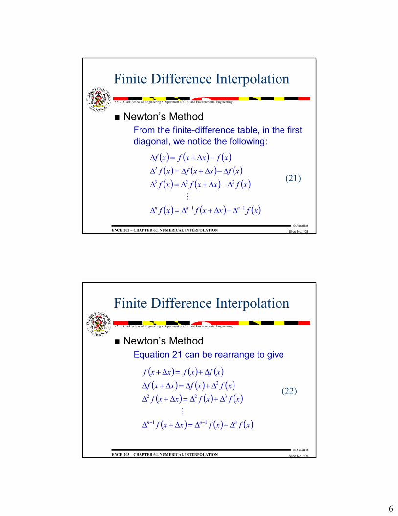
� Newton�s MethodFrom the finite-difference table, in the first diagonal, we notice the following:
( ) ( ) ( )( ) ( ) ( )( ) ( ) ( )
( ) ( ) ( )xfxxfxf
xfxxfxfxfxxfxf
xfxxfxf
nnn 11
223
2
−− ∆−∆+∆=∆
∆−∆+∆=∆∆−∆+∆=∆
−∆+=∆
M
(21)
© Assakkaf
Slide No. 109
� A. J. Clark School of Engineering � Department of Civil and Environmental Engineering
ENCE 203 � CHAPTER 6d. NUMERICAL INTERPOLATION
Finite Difference Interpolation
� Newton�s MethodEquation 21 can be rearrange to give
( ) ( ) ( )( ) ( ) ( )( ) ( ) ( )
( ) ( ) ( )xfxfxxf
xfxfxxfxfxfxxf
xfxfxxf
nnn ∆+∆=∆+∆
∆+∆=∆+∆∆+∆=∆+∆
∆+=∆+
−− 11
322
2
M
(22)
7
© Assakkaf
Slide No. 110
� A. J. Clark School of Engineering � Department of Civil and Environmental Engineering
ENCE 203 � CHAPTER 6d. NUMERICAL INTERPOLATION
Finite Difference Interpolation
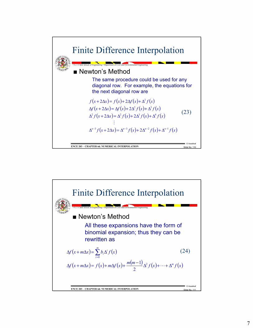
� Newton�s MethodThe same procedure could be used for any diagonal row. For example, the equations for the next diagonal row are
( ) ( ) ( ) ( )( ) ( ) ( ) ( )( ) ( ) ( ) ( )
( ) ( ) ( ) ( )xfxfxfxxf
xfxfxfxxfxfxfxfxxf
xfxfxfxxf
nnnn 1233
4322
32
2
22
2222
22
−−−− ∆+∆+∆=∆+∆
∆+∆+∆=∆+∆∆+∆+∆=∆+∆
∆+∆+=∆+
M
(23)
© Assakkaf
Slide No. 111
� A. J. Clark School of Engineering � Department of Civil and Environmental Engineering
ENCE 203 � CHAPTER 6d. NUMERICAL INTERPOLATION
Finite Difference Interpolation
� Newton�s MethodAll these expansions have the form of binomial expansion; thus they can be rewritten as
( ) ( )
( ) ( ) ( ) ( ) ( ) ( )xfxfmmxfmxfxmxf
xfbxmxf
m
m
i
ii
∆++∆−+∆+=∆+∆
∆=∆+∆ ∑=
L2
0
21
(24)
8
© Assakkaf
Slide No. 112
� A. J. Clark School of Engineering � Department of Civil and Environmental Engineering
ENCE 203 � CHAPTER 6d. NUMERICAL INTERPOLATION
Finite Difference Interpolation
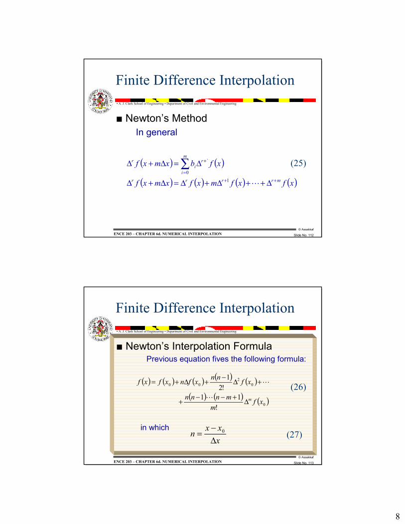
� Newton�s MethodIn general
( ) ( )
( ) ( ) ( ) ( )xfxfmxfxmxf
xfbxmxf
mrrrr
m
i
ri
r
++
=
+
∆++∆+∆=∆+∆
∆=∆+∆ ∑L1
0
` (25)
© Assakkaf
Slide No. 113
� A. J. Clark School of Engineering � Department of Civil and Environmental Engineering
ENCE 203 � CHAPTER 6d. NUMERICAL INTERPOLATION
Finite Difference Interpolation
� Newton�s Interpolation FormulaPrevious equation fives the following formula:
in which
( ) ( ) ( ) ( ) ( )( ) ( ) ( )0
02
00
!11
!21
xfm
mnnn
xfnnxfnxfxf
m∆+−−+
+∆−+∆+=
L
L
xxxn
∆−
= 0
(26)
(27)
9
© Assakkaf
Slide No. 114
� A. J. Clark School of Engineering � Department of Civil and Environmental Engineering
ENCE 203 � CHAPTER 6d. NUMERICAL INTERPOLATION
Finite Difference Interpolation
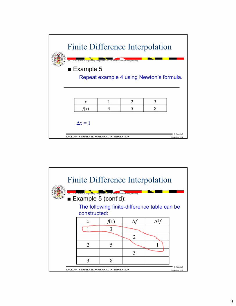
� Example 5Repeat example 4 using Newton�s formula.
853f(x)321x
∆x = 1
© Assakkaf
Slide No. 115
� A. J. Clark School of Engineering � Department of Civil and Environmental Engineering
ENCE 203 � CHAPTER 6d. NUMERICAL INTERPOLATION
Finite Difference Interpolation
� Example 5 (cont�d):The following finite-difference table can be constructed:
833
1522
31∆2f∆ff(x)x
10
© Assakkaf
Slide No. 116
� A. J. Clark School of Engineering � Department of Civil and Environmental Engineering
ENCE 203 � CHAPTER 6d. NUMERICAL INTERPOLATION
Finite Difference Interpolation
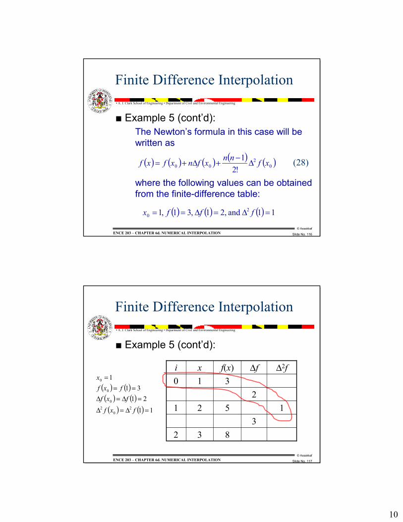
� Example 5 (cont�d):The Newton�s formula in this case will be written as
where the following values can be obtained from the finite-difference table:
( ) ( ) ( ) ( ) ( )02
00 !21 xfnnxfnxfxf ∆−+∆+=
( ) ( ) ( ) 11 and ,21 ,31 ,1 20 =∆=∆== fffx
(28)
© Assakkaf
Slide No. 117
� A. J. Clark School of Engineering � Department of Civil and Environmental Engineering
ENCE 203 � CHAPTER 6d. NUMERICAL INTERPOLATION
Finite Difference Interpolation
� Example 5 (cont�d):
2
1
0i
833
1522
31∆2f∆ff(x)x
( ) ( )( ) ( )( ) ( ) 11
2131
1
20
2
0
0
0
=∆=∆
=∆=∆==
=
fxffxf
fxfx
11
© Assakkaf
Slide No. 118
� A. J. Clark School of Engineering � Department of Civil and Environmental Engineering
ENCE 203 � CHAPTER 6d. NUMERICAL INTERPOLATION
Finite Difference Interpolation
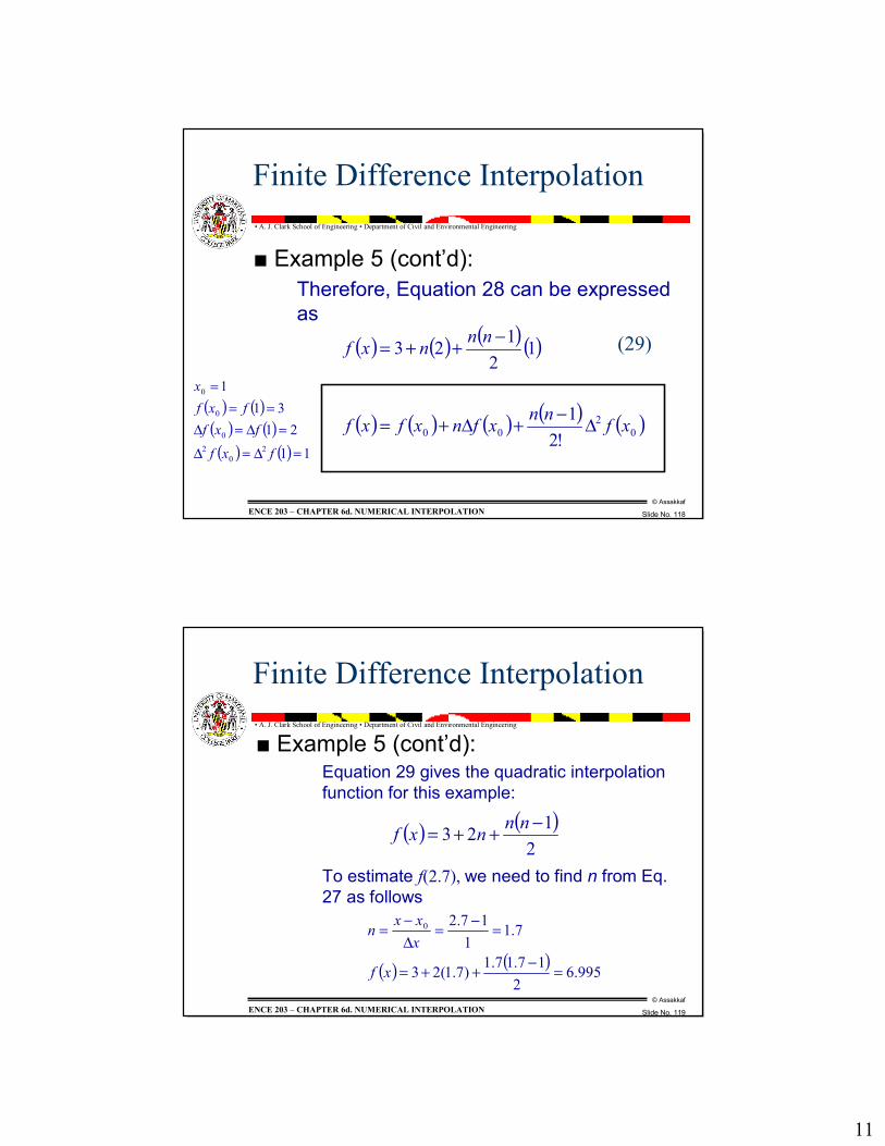
� Example 5 (cont�d):Therefore, Equation 28 can be expressed as
( ) ( ) ( )( )
( ) ( ) ( ) ( ) ( )02
00 !21
12
123
xfnnxfnxfxf
nnnxf
∆−+∆+=
−++=
( ) ( )( ) ( )( ) ( ) 11
2131
1
20
20
0
0
=∆=∆
=∆=∆==
=
fxffxf
fxfx
(29)
© Assakkaf
Slide No. 119
� A. J. Clark School of Engineering � Department of Civil and Environmental Engineering
ENCE 203 � CHAPTER 6d. NUMERICAL INTERPOLATION
Finite Difference Interpolation
� Example 5 (cont�d):Equation 29 gives the quadratic interpolation function for this example:
To estimate f(2.7), we need to find n from Eq. 27 as follows
( ) ( ) 995.62
17.17.1)7.1(23
7.11
17.20
=−++=
=−=∆−
=
xf
xxxn
( ) ( )2
123 −++= nnnxf
12
© Assakkaf
Slide No. 120
� A. J. Clark School of Engineering � Department of Civil and Environmental Engineering
ENCE 203 � CHAPTER 6d. NUMERICAL INTERPOLATION
Finite Difference Interpolation
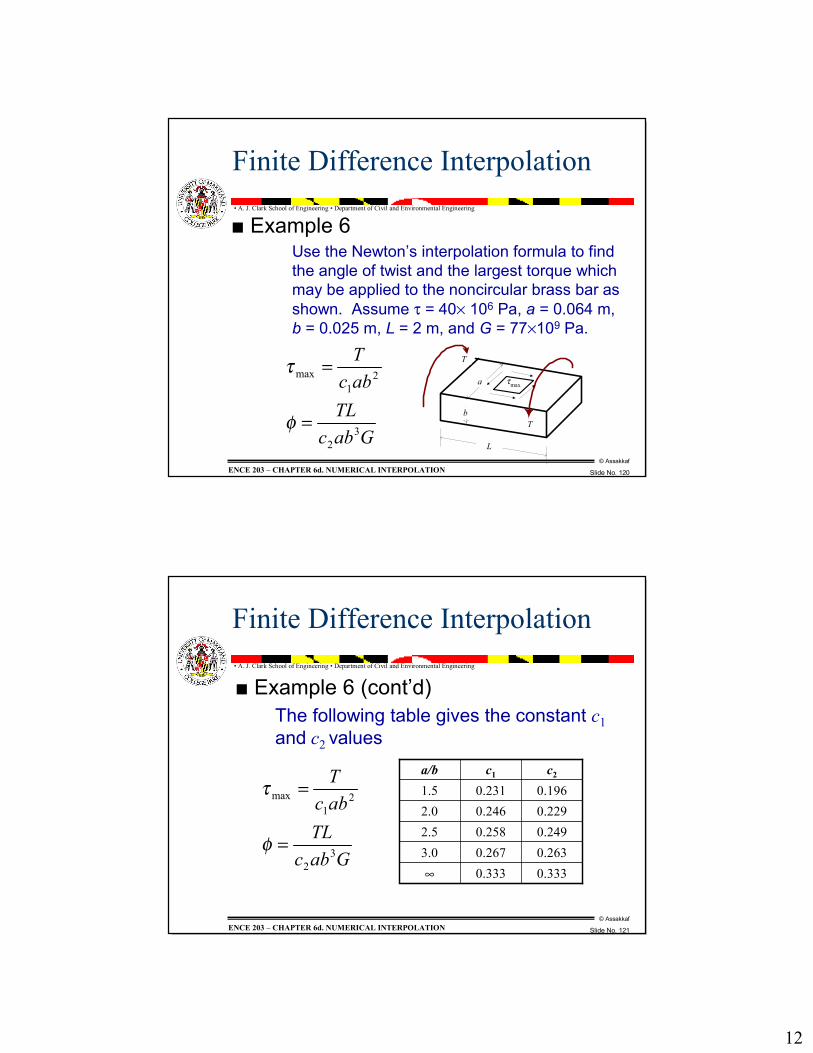
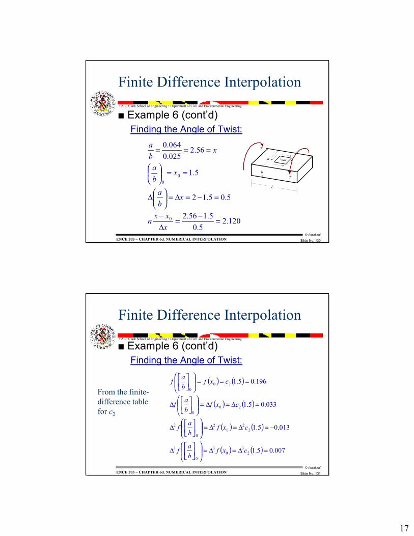
� Example 6Use the Newton�s interpolation formula to find the angle of twist and the largest torque which may be applied to the noncircular brass bar as shown. Assume τ = 40× 106 Pa, a = 0.064 m, b = 0.025 m, L = 2 m, and G = 77×109 Pa.
a
b
T
T
L
τmax
GabcTL
abcT
32
21
max
=
=
φ
τ
© Assakkaf
Slide No. 121
� A. J. Clark School of Engineering � Department of Civil and Environmental Engineering
ENCE 203 � CHAPTER 6d. NUMERICAL INTERPOLATION
Finite Difference Interpolation
� Example 6 (cont�d)The following table gives the constant c1and c2 values
0.3330.333∞0.2630.2673.00.2490.2582.50.2290.2462.00.1960.2311.5c2c1a/b
GabcTL
abcT
32
21
max
=
=
φ
τ
13
© Assakkaf
Slide No. 122
� A. J. Clark School of Engineering � Department of Civil and Environmental Engineering
ENCE 203 � CHAPTER 6d. NUMERICAL INTERPOLATION
Finite Difference Interpolation
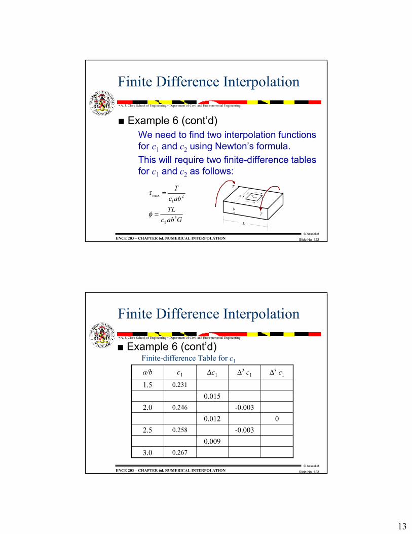
� Example 6 (cont�d)We need to find two interpolation functions for c1 and c2 using Newton�s formula.This will require two finite-difference tables for c1 and c2 as follows:
a
b
T
T
L
τmax
GabcTL
abcT
32
21
max
=
=
φ
τ
© Assakkaf
Slide No. 123
� A. J. Clark School of Engineering � Department of Civil and Environmental Engineering
ENCE 203 � CHAPTER 6d. NUMERICAL INTERPOLATION
Finite Difference Interpolation
� Example 6 (cont�d)
0.2673.00.009
-0.0030.2582.500.012
-0.0030.2462.00.015
0.2311.5
∆3 c1∆2 c1∆c1c1a/b
Finite-difference Table for c1
14
© Assakkaf
Slide No. 124
� A. J. Clark School of Engineering � Department of Civil and Environmental Engineering
ENCE 203 � CHAPTER 6d. NUMERICAL INTERPOLATION
Finite Difference Interpolation
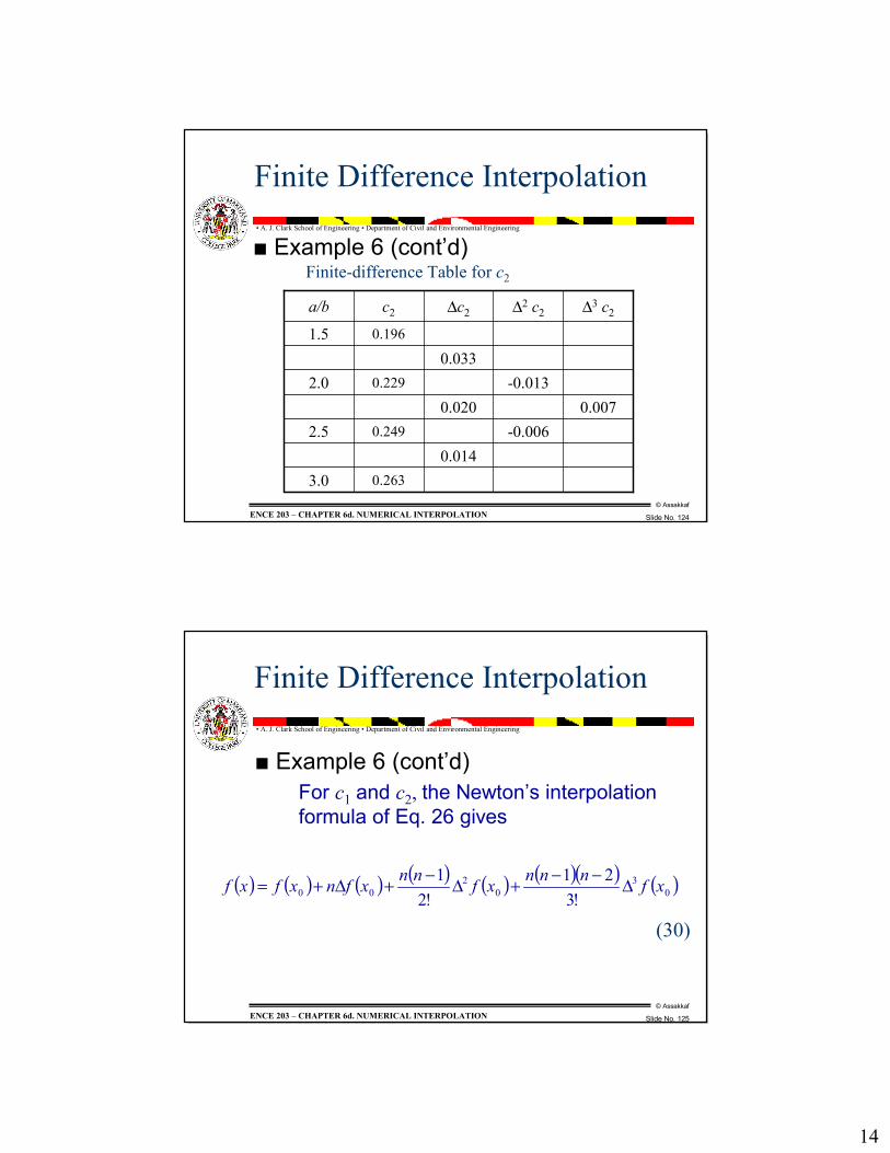
� Example 6 (cont�d)
0.2633.00.014
-0.0060.2492.50.0070.020
-0.0130.2292.00.033
0.1961.5
∆3 c2∆2 c2∆c2c2a/b
Finite-difference Table for c2
© Assakkaf
Slide No. 125
� A. J. Clark School of Engineering � Department of Civil and Environmental Engineering
ENCE 203 � CHAPTER 6d. NUMERICAL INTERPOLATION
Finite Difference Interpolation
� Example 6 (cont�d)For c1 and c2, the Newton�s interpolation formula of Eq. 26 gives
( ) ( ) ( ) ( ) ( ) ( )( ) ( )03
02
00 !321
!21 xfnnnxfnnxfnxfxf ∆−−+∆−+∆+=
(30)
15
© Assakkaf
Slide No. 126
� A. J. Clark School of Engineering � Department of Civil and Environmental Engineering
ENCE 203 � CHAPTER 6d. NUMERICAL INTERPOLATION
Finite Difference Interpolation
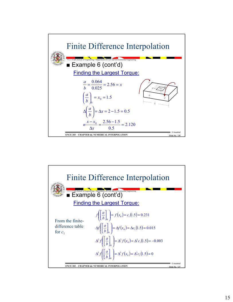
� Example 6 (cont�d)Finding the Largest Torque:
120.25.0
5.156.2
5.05.12
5.1
56.2025.0064.0
0
00
=−=∆−
=−=∆=
∆
==
===
xxxn
xba
xba
xba
a
b
T
T
L
τmax
© Assakkaf
Slide No. 127
� A. J. Clark School of Engineering � Department of Civil and Environmental Engineering
ENCE 203 � CHAPTER 6d. NUMERICAL INTERPOLATION
Finite Difference Interpolation
� Example 6 (cont�d)Finding the Largest Torque:
( ) ( )
( ) ( )
( ) ( )
( ) ( ) 05.1
003.05.1
015.05.1
231.05.1
13
03
0
3
12
02
0
2
100
100
=∆=∆=
∆
−=∆=∆=
∆
=∆=∆=
∆
===
cxfbaf
cxfbaf
cxfbaf
cxfbaf
From the finite-difference table for c1
16
© Assakkaf
Slide No. 128
� A. J. Clark School of Engineering � Department of Civil and Environmental Engineering
ENCE 203 � CHAPTER 6d. NUMERICAL INTERPOLATION
Finite Difference Interpolation
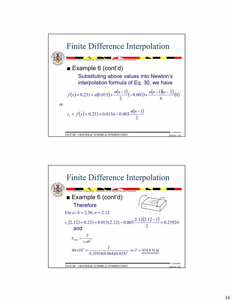
� Example 6 (cont�d)Substituting above values into Newton�s interpolation formula of Eq. 30, we have
( ) ( ) ( )( ) ( )( )( )
( ) ( )2
1003.0015.0231.0
or
06
21003.02
1015.0231.0
1−−+==
−−+−−++=
nnnxfc
nnnnnnxf
© Assakkaf
Slide No. 129
� A. J. Clark School of Engineering � Department of Civil and Environmental Engineering
ENCE 203 � CHAPTER 6d. NUMERICAL INTERPOLATION
Finite Difference Interpolation
� Example 6 (cont�d)Therefore
and( ) ( ) 25924.0
2112.212.2003.0)12.2(015.0231.012.2
12.2 ,56.2/For
1 =−−+=
==
c
nba
N.m 8.414)025.0)(064.0(25924.0
1040 26
21
max
=⇒=×
=
TTabcTτ
a
b
T
T
L
τmax
17
© Assakkaf
Slide No. 130
� A. J. Clark School of Engineering � Department of Civil and Environmental Engineering
ENCE 203 � CHAPTER 6d. NUMERICAL INTERPOLATION
Finite Difference Interpolation
� Example 6 (cont�d)Finding the Angle of Twist:
120.25.0
5.156.2
5.05.12
5.1
56.2025.0064.0
0
00
=−=∆−
=−=∆=
∆
==
===
xxxn
xba
xba
xba
a
b
T
T
L
τmax
© Assakkaf
Slide No. 131
� A. J. Clark School of Engineering � Department of Civil and Environmental Engineering
ENCE 203 � CHAPTER 6d. NUMERICAL INTERPOLATION
Finite Difference Interpolation
� Example 6 (cont�d)Finding the Angle of Twist:
( ) ( )
( ) ( )
( ) ( )
( ) ( ) 007.05.1
013.05.1
033.05.1
196.05.1
23
03
0
3
22
02
0
2
200
200
=∆=∆=
∆
−=∆=∆=
∆
=∆=∆=
∆
===
cxfbaf
cxfbaf
cxfbaf
cxfbaf
From the finite-difference table for c2
18
© Assakkaf
Slide No. 132
� A. J. Clark School of Engineering � Department of Civil and Environmental Engineering
ENCE 203 � CHAPTER 6d. NUMERICAL INTERPOLATION
Finite Difference Interpolation
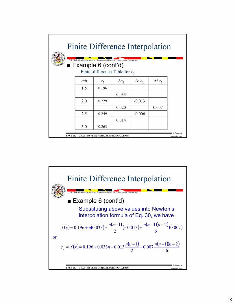
� Example 6 (cont�d)
0.2633.00.014
-0.0060.2492.50.0070.020
-0.0130.2292.00.033
0.1961.5
∆3 c2∆2 c2∆c2c2a/b
Finite-difference Table for c2
© Assakkaf
Slide No. 133
� A. J. Clark School of Engineering � Department of Civil and Environmental Engineering
ENCE 203 � CHAPTER 6d. NUMERICAL INTERPOLATION
Finite Difference Interpolation
� Example 6 (cont�d)Substituting above values into Newton�s interpolation formula of Eq. 30, we have
( ) ( ) ( )( ) ( )( )( )
( ) ( ) ( )( )6
21007.02
1013.0033.0196.0
or
007.06
21013.02
1033.0196.0
2−−+−−+==
−−+−−++=
nnnnnnxfc
nnnnnnxf
19
© Assakkaf
Slide No. 134
� A. J. Clark School of Engineering � Department of Civil and Environmental Engineering
ENCE 203 � CHAPTER 6d. NUMERICAL INTERPOLATION
Finite Difference Interpolation
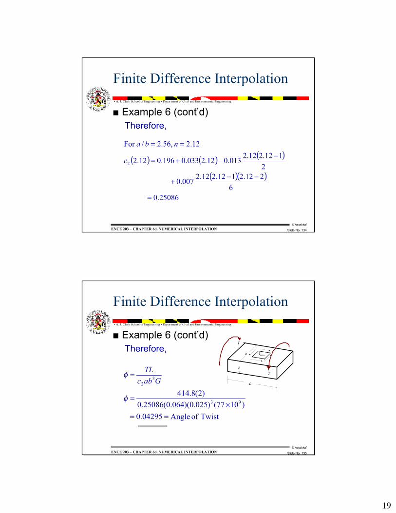
� Example 6 (cont�d)Therefore,
( ) ( ) ( )
( )( )
25086.0 6
212.2112.212.2007.0
2112.212.2013.012.2033.0196.012.2
12.2 ,56.2/For
2
=
−−+
−−+=
==
c
nba
© Assakkaf
Slide No. 135
� A. J. Clark School of Engineering � Department of Civil and Environmental Engineering
ENCE 203 � CHAPTER 6d. NUMERICAL INTERPOLATION
Finite Difference Interpolation
� Example 6 (cont�d)Therefore,
Twist of Angle04295.0 )1077()025.0)(064.0(25086.0
)2(8.41493
32
==×
=
=
φ
φGabc
TL
a
b
T
T
L
τmax
20
© Assakkaf
Slide No. 136
� A. J. Clark School of Engineering � Department of Civil and Environmental Engineering
ENCE 203 � CHAPTER 6d. NUMERICAL INTERPOLATION
Lagrange Polynomials
� Lagrange interpolation polynomials are useful when the given data contains unequal intervals for the independent variables x.
� In fact, this is the case for many engineering problems.
� The data collection cannot be controlled.
© Assakkaf
Slide No. 137
� A. J. Clark School of Engineering � Department of Civil and Environmental Engineering
ENCE 203 � CHAPTER 6d. NUMERICAL INTERPOLATION
Lagrange Polynomials
� The data are collected for one variables f(x), which is the independent variables, as a function of second variable x.
� In the Newton�s interpolation formula, the independent variable x was assumed to be measured at a constant interval, ∆x.
� Lagrange method can handled problem with a varying ∆x.
21
© Assakkaf
Slide No. 138
� A. J. Clark School of Engineering � Department of Civil and Environmental Engineering
ENCE 203 � CHAPTER 6d. NUMERICAL INTERPOLATION
Lagrange Polynomials
� DefinitionThe Lagrange interpolation polynomial is simply a reformulation of Newton�s polynomial that avoids the computation using finite difference, and that can handled problems with varying interval.
© Assakkaf
Slide No. 139
� A. J. Clark School of Engineering � Department of Civil and Environmental Engineering
ENCE 203 � CHAPTER 6d. NUMERICAL INTERPOLATION
Lagrange Polynomials
� Definition of Terms� The data sample is assumed to consist of n
pairs of values measured on x and f(x), with xi being the ith measured value of the independent variable.
� The method provides an estimate of the value of f(x) at a specified value of x, which is denoted x0.
22
© Assakkaf
Slide No. 140
� A. J. Clark School of Engineering � Department of Civil and Environmental Engineering
ENCE 203 � CHAPTER 6d. NUMERICAL INTERPOLATION
Lagrange Polynomials
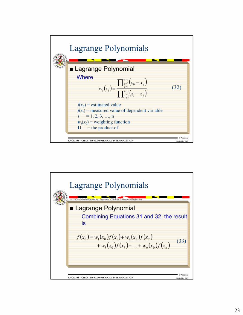
� Definition of Termsf(x0) = estimated valuef(xi) = measured value of dependent variablei = 1, 2, 3, �, nThe method involves a weighting function, with
the weight given to the ith value of f for x0denoted as wi(x0).
© Assakkaf
Slide No. 141
� A. J. Clark School of Engineering � Department of Civil and Environmental Engineering
ENCE 203 � CHAPTER 6d. NUMERICAL INTERPOLATION
Lagrange Polynomials
� Lagrange PolynomialThe Lagrange interpolating polynomial for estimating the value of f(x0) is given by
( ) ( ) ( )∑=
=n
iii xfxwxf
100
(31)
23
© Assakkaf
Slide No. 142
� A. J. Clark School of Engineering � Department of Civil and Environmental Engineering
ENCE 203 � CHAPTER 6d. NUMERICAL INTERPOLATION
Lagrange Polynomials
� Lagrange PolynomialWhere
( )( )( )∏
∏−
≠=
−
≠=
−
−= 1
1
11 0
n
ijj ji
n
ijj j
iixx
xxxw (32)
f(x0) = estimated valuef(xi) = measured value of dependent variablei = 1, 2, 3, �, nwi(x0) = weighting functionΠ = the product of
© Assakkaf
Slide No. 143
� A. J. Clark School of Engineering � Department of Civil and Environmental Engineering
ENCE 203 � CHAPTER 6d. NUMERICAL INTERPOLATION
Lagrange Polynomials
� Lagrange PolynomialCombining Equations 31 and 32, the result is
( ) ( ) ( ) ( ) ( )( ) ( ) ( ) ( )nn xfxwxfxw
xfxwxfxwxf
0303
2021010
++++=
K(33)