403

CHAPTER 7

AGGREGATION OF DISAGGREGATE MODELS FOR FORECASTING

To be useful in planning and policy analysis, forecasts of individual choicebehavior must be aggregated into geographic, socioeconomic, or supply marketgroups of interest to the planner. Disaggregate models are usually non-linear inexplanatory variables, and groups for which forecasts are needed arenon-homogeneous in these variables. Hence, the aggregation process isnon-linear, and must take into account the distribution of the explanatoryvariables. Group choice shares are generally not equal to the probability of choicean individual with the average explanatory variables of the group would have. The choice probabilities of individuals in the multinomial logit model, and otherchoice models used in this study, can be written in the general form

(l) Pj = Fj(V1,...,Vj) ,

where Pj = probability of choosing alternative j ;

Vj = "mean" utility of alternative j ;

J = number of alternatives;

and the utility Vj is a function of observed socioeconomic characteristics andlevel-of-service attributes of alternative j ,

(2) Vj = v(LOSj,SE) .

1Koppelman (1975, 1976) referred to this method as integration/summation.

404

Typically, the function (2) is taken to be linear in specified functions oflevel-of-service and socioeconomic variables,

(3) Vj � �K

k�1βkZ

k(LOSj,SE) ,

with the βk interpreted as "importance weights" that are estimated in the demandanalysis. Let zjk = Zk (LOSj,SE) , and define zjk to be the group mean of zjk .Then group average utilities satisfy

(4) V j � �K

k�1βkz jk .

A naive aggregate forecast can be obtained by substituting in (l) . However,Vj

non-linearity of the function (l) implies that in general the probability evaluated ataverage utilities of the group will not equal the group choice probabilities (i.e., theaverage of the individual probabilities). Consequently, the naive procedure will ingeneral yield biased forecasts.

If, for a group, the multivariate distribution of the utilities Vj is known,and denoted by g(V1,...,Vj) , then the aggregate probability for the group satisfies

(5) Pj � � Fj(V1,...,Vj) g(V1,...,VJ) dV1...dVJ .

This is termed aggregation by statistical integration.1 For a finite (but usuallylarge) group size, this formula reduces to sum

1Overall error is measured in terms of the root-mean-square of the errors in the separate alternatives withrespect to the equivalent enumerated aggregate forecast. See equation (10) in this chapter.

405

(6) Pj �1N �

N

n�1Fj(Vln,...,VJn) ,

where Vjn is the utility of alternative j for individual n . This is known as anenumerated aggregate forecast.

There is an aggregation problem because the enumeration (6) can beexpensive, especially for forecasts for groups such as interzonal choice matrices.Nor is the expected value computation (5) practical in most cases. g(V1,...,Vj) isneither simple nor easy to obtain, and the integral (5) has a known analyticalsolution for only one special case (McFadden and Reid, 1975).

Other attempts to evaluate (5) have also been impractical. Westintransforms (5) to distributions in probability space. However, his method appliesonly to binary choice, and requires numerical integration procedures as costly asenumeration (Westin, 1974).

An attempt by Talvitie to approximate the expected value of group sharesby a Taylor series has given counter-productive results for typical variances of theexplanatory variables because of the poor convergence properties of seriesexpansion (Talvitie, 1973; Koppelman, 1975).

The aggregation error that results from naive aggregate forecasts can besubstantial. A study on a Washington, D. C. area sample and model ofCBD-oriented work mode-choice has shown this error to range from eight to tenpercent RMS, depending on the geographic level of aggregation (Koppelman,1976).1 Results on the data and models of the Urban Travel Demand ForecastingProject study show naive forecasting error between 13.8 RMS, for origin zoneaggregate trips, and forty-three percent RMS for metropolitan area trips,respectively. Neither of the studies were for interzonal naive aggregation, thoughit is estimated that for this level of geographic interchange forecasting the errorwill be about half the origin zone level error above, on the average, andconsiderably greater for individual interchanges (see Vol. VII, Chapter 7, Table7.3 discussion).

406

Naive aggregation can produce larger biases than are produced byestimating and forecasting with strictly aggregate data. The latter procedure has,at least, the ability to replicate baseline shares. However, strictly aggregatemodels produce biased predictions of the impacts of most policy changes and areinsensitive to many policy tests of interest.

The essential advantage of disaggregate models is that they are sensitive tothe mix of variables explaining a traveler�s choice. Ignoring the distribution ofthese variables in forecasting produces errors that cancel the advantage of themodels. Disaggregate models and an acceptable aggregation method must be usedto gain accurate forecasts.

Fortunately, some progress has been made in approximations toenumerated aggregate forecasts, based on classification. These approximationsare simple and considerably reduce the error of the naive method. Koppelman(1976) has shown that classification by auto availability and choice set can reduceRMS error (at various levels of aggregation) to three percent versus eight percentby the naive method. Later results on a sample used by this study show thatclassification based on the values of differences in utilities of choices can reduceerror to less than one percent compared to forty percent for the naive method.

The classification methods also have great potential savings incomputation efficiency with suitably chosen classes. Their attempts to delineatedifferent choice types approach the minimum amount of information necessary todefine the different market segments or traveler types making up the range ofpossible choices. Examples and recommended practice with these methods willbe explained in detail following a review of the state of aggregation theory and adiscussion of the planning context, its needs, and resources. Questions of dataneed and availability, efficiency of predictions, and effects of aggregate size willbe discussed in addition to accuracy.

407

The State of Aggregation Theory

The major thrusts in simplifying the general theory of aggregation have notbeen as fruitful as the approximate classification approaches. Koppelman (1975)extended Talvitie�s Taylor series approximation method for multiple choices toaccount for covariances between utilities of different alternatives. The aggregateshares are

(7) �����Sj

N� P(j | V) �

12�

J

K�

J

�

�2P(i | V)�VK�V

� V

cov (VK,V�) � ... ,

where J is the number of alternatives, V is the vector of utilities of the choices, is its mean in the aggregate of N travelers, and VK,V

� are the utilities ofV

choices k and � . However, he found that this approximation suffers from largererrors when the series is truncated after the second term than when it is truncatedafter the first term. That is, the method produces worse results than the naiveapproach for aggregate sizes down to districts that were about l/l00th of theWashington metropolitan population.

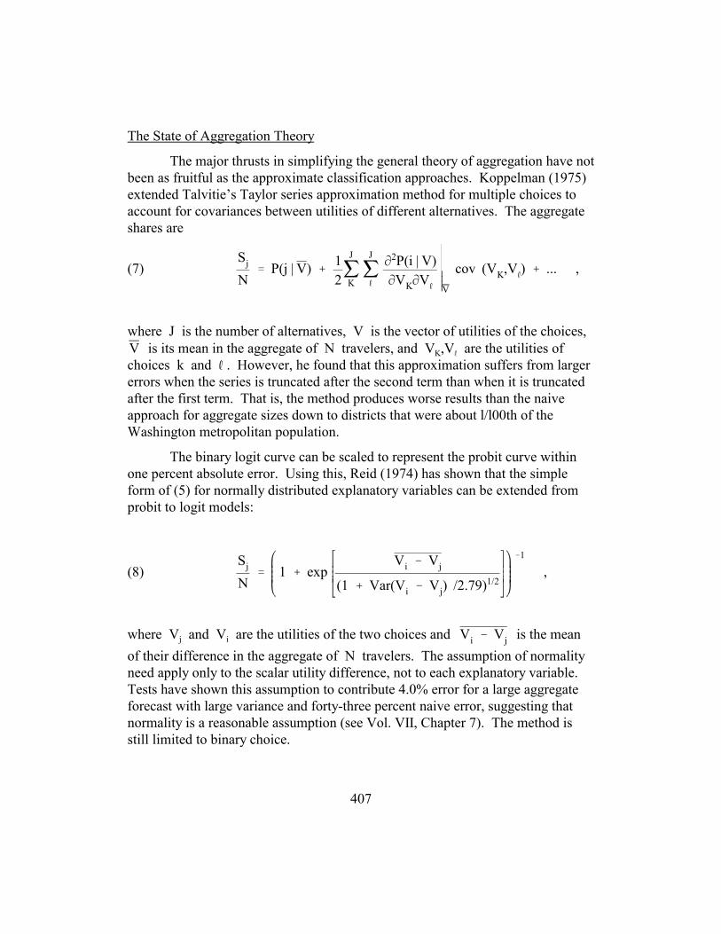
The binary logit curve can be scaled to represent the probit curve withinone percent absolute error. Using this, Reid (1974) has shown that the simpleform of (5) for normally distributed explanatory variables can be extended fromprobit to logit models:

(8)Sj

N� 1 � exp

Vi � Vj

(1 � Var(Vi � Vj) /2.79)1/2

�1

,

where Vj and Vi are the utilities of the two choices and is the meanVi � Vj

of their difference in the aggregate of N travelers. The assumption of normalityneed apply only to the scalar utility difference, not to each explanatory variable.Tests have shown this assumption to contribute 4.0% error for a large aggregateforecast with large variance and forty-three percent naive error, suggesting thatnormality is a reasonable assumption (see Vol. VII, Chapter 7). The method isstill limited to binary choice.

408

Work on the theory of multiple choice by the integration method could bevery productive in extending its simplicity and accuracy. Recent research onestimation methods for multinomial probit models has had the side-effect ofrevealing new efficient approximations to integrals of the form of (5). (Daganzo,et al., 1976; McFadden, 1977).

An aggregate forecast by classification can be defined as a weighted sumof the naive shares in classes identified by some characteristics of the travelers ortheir alternatives. The aggregate shares are obtained by

(9)Sj

N� �

C

c�1P(j | Vc)

Nc

N,

where c is the index of the C cells in the classification, is the mean utilityVc

computed for cell c , and Nc is the number of travelers in cell c . Koppelman(1975) has done the principal study of aggregation by classification using choicesubsets and specific variable values as identifiers. He found that where the fullalternative set is unavailable to a significant portion of individuals in theaggregate (thirty percent in his tests) that classification based on available choiceset is more effective than on any single variable. Additional classification byvariables is recommended to concentrate on those with greatest contribution to theutility variance. Choice set classifications reduced RMS error in the Washingtonsample to five percent. Cross-classification with the variable auto/drivers in thehousehold reduced error to three percent regardless of aggregate size. Naivemethod error was eight percent. No other methods tested by Koppelsnan gavesmaller error. He did not test the statistical integration method.

As stated before, the statistical integration method has been found in thisstudy to be capable of reducing naive error over ten-fold. Koppelman performedMonte Carlo simulations of the aggregation error by each of the above methods todetermine the range of error with statistics of the distribution of the utilities of thealternatives. These confirmed that the integration and classification methodsusually gave better results than the naive and series approximation methods,agreeing with his empirical results, and with ours. However, the simulationsshow that for skewed distributions, exceptions may occur to this ranking,especially regarding the desirability of the integration method.

409

Results of this study have extended the general classification approach intwo ways--developing more systematic methods for defining classes based onspecific variables and considering classification directly on utility scale values.

A systematic picture of priorities for class identifier variables can begained by looking at the covariance matrices of the within-aggregate variation ofthe explanatory variables at the desired level of aggregation. The binary choiceaggregation theory has established the direct relationship between this matrix andaggregate shares for probit models and for logit models with limited assumptions.Though no corresponding theoretical relationship exists in the multiple choicecase, the covariance matrices are still better indicators of which variables areappropriate classifiers than a priori knowledge, especially if these vary withaggregate level. Table 68 shows a normalized covariance matrix of the intra-cityaggregate values of the major explanatory variables in two alternatives of aprediction model. The model used is shown in Part II, Chapter 2, Table 12 of thisvolume. The covariance elements are normalized by dividing by the largest oftheir values (in this case it is the variance of the utility of CARS/DRIVERS in thetraveler's household) in order to give a picture of the ranking of the contributionsof each variable to the overall utility variance. The underlying model is a logitfunction, linear in its explanatory variables.

410

TAB

LE 6

8C

ovar

ianc

e M

atrix

of I

ntra

-City

Val

ues o

f Exp

lana

tory

Var

iabl

es

Aut

o-A

lone

Alte

rnat

ive

Var

iabl

esB

us-w

ith-W

alk-

Acc

essA

ltern

ativ

e

Driv

ers

AU

TO-

ON

VEH

Driv

ers

Empl

oym

.D

ens.

Cos

tB

usw

alk

Bus

-O

NV

EHH

dway

Xfe

r-w

ait

Sum

Alt.

2=1.

73

C/D

R1.

0.0

6<

<.0

7<

<<

<

AO

NV

.06

.51

<<

-.07

.23

<.0

6

DR

�s<

<.2

7<

<<

EMP

<.1

0<

.11

-.06

<

CO

ST1

.07

.10

.07

<

BW

LK<

-.07

<-.0

6.8

4.3

3.0

5<

.84

BO

NV

<.2

3<

<.3

3.2

1<

.07

.54

HD

W<

<<

.05

<.0

9<

.14

XFT

<.0

6<

.07

<.1

4.2

1

SUM

Alt.

1= 2

.62

1.26

.91

.27

.11

.07

4.35

3.96

3

NO

TES:

1.C

ovar

ianc

e va

lues

are

nor

mal

ized

by

mul

tiply

ing

by th

eir r

espe

ctiv

e m

odel

coe

ffic

ient

s and

div

idin

g by

the

max

imum

such

"util

ity"

cova

rianc

e el

emen

t:

(in

this

cas

e th

e m

axim

um u

tility

com

pone

nt c

ovar

ianc

e is

the

varia

nce

of th

eβ k

S2 k�β �

/β1S

2 11β 1

first

var

iabl

e C

AR

S/D

RIV

ERS)

.

2<

= el

emen

t is l

ess t

han

.05

.

3.To

tal v

aria

nce

of d

iffer

ence

s in

utili

ty b

etw

een

alte

rnat

ives

1 a

nd 2

.

1Because most of the variables in this model are unique to a mode, variances of intermodal utility differencesare equal to the individual modal elements. Where the same variable appears in the utility expression for twomodes, the differences of utilities can be obtained from the table by the expression for the variance of such adifference: Var (X - Y) = Var X + Var Y - 2 Cov (X,Y).

411

Hence, each element in the matrix is the product of the covariances of theindividual variables and their correponding model coefficients

; k and � are the matrix indices of the K variables in theSk� � βkS2k�β� / β1S

211β1

model, 1 < k, � < K ; βkβ� are the linear utility coefficients for the k-th and �-th

variables; is the sample covariance between the k and �-th variables; and S 2k�

is the corresponding utility variance for the largest matrix element. Theseβ1S211β1

elements are called utility component covariances because each expresses the partof the total sample variance of the linear utility for one mode contributed by asingle variable (diagonal variance elements) or pairs of variables (covarianceelements). The sum of the matrix elements for any mode equals the total varianceof the utility for that mode.

For binary logit choice models the relationship between these covariancesand aggregation error is understood under the assumption of normally-distributedexplanatory variables (equation (8 )). Thus Table 68 provides a convenient way torank the individual variables and their combinations, by their importance forreducing aggregation error for binary choice. The larger the variance of thedifference of utilities between the two modes the larger the aggregation error.1

The variables that have individual values that are most important forreducing aggregation are the ones with the largest values in Table 68, such asBUSWALK, CARS/DRIVERS, and AONVEH (time riding in autos). Theinter-modal covariances show the relative importance of these pairs of variables inaggregation. However, because inter-modal elements contribute to the variance ofbinary utility difference with negative sign it is the negative values such as thatbetween CARS/ DRIVERS and BUSWALK that increase the aggregationcorrection. Positive values indicate a compensating reduction in aggregationerror. The amount of aggregation error that will result in a forecast using theindividual values of only selected variables can be estimated by comparingequation (8) with and without the unnormalized values of the matrix elements to

1Only the individual values of some variables or their variance may be available in a forecasting situation. Insome cases, variances are possible to obtain or estimate where covariances are not Talvitie and Dehghani,1976).

412

be considered.1

Inspection of Table 68 shows that a large part of the variance of theutilities, and hence aggregation correction, can be recovered by considering only afew of the variables in the model. For example, three of the eleven variables inthe model used here--CARS/DRIVER, BUSWALK, and BONVEH (riding onbus)--constitute fifty-nine percent of the utility variance. When only theirindividual values are used for prediction, they correct for sixty-nine percent of theaggregation error produced by the naive method. Auto (AONVEH) time, incontrast, contributes nothing to the correction of aggregation error by its inclusionwith this set since its covariance with BUSWALK cancels out its variancecontribution alone.

The covariance matrix alone gives incomplete information on theadvantage gained in classification because of the correlations between theclassifier variable(s) and the others. This can also be evaluated by adding theinformation from a corresponding correlation matrix of the variables within thesame prediction aggregate. The additional power of a classifier due to this effectis given by the sum of the product of covariances and correlation coefficients ofall variables correlated to the classifier. With this procedure, one can minimizeaggregation error, given limits on the number of classification variables, orminimize the number of classifiers, given tolerable limits on error.

When applying this covariance analysis to multiple choice, simplerapproximate guides to the important aggregation variables can be gained byobserving the covariance matrices of major subsets of the alternatives. Theseshould be alternatives which have shares different from 1/J and are considerablydifferent from one another.

The procedure also does not account for skewed utility distributions.Skewedness will weaken the analysis. This does not appear be a problem in thetests of this study (see Vol. VII).

The covariance analysis on a subsample of the population can also guidelarger sample data collection and processing priorities for planning and policyanalysis.

413

Utility Scale Classification

Though the covariance analysis procedure above can systematically guideselection of classification variables, the process is inefficient. If more than a fewvariables contribute significantly to aggregation variance, the number ofcross-classifications becomes large for achievement of small error. This isespecially true of predictions for large geographic aggregates.

A more efficient method of classification is possible for the class of simplyscalable models of the form of equation (1). These models express choice among J alternatives as a function of J utility scales of the individual decision-maker�scharacteristics and choice attributes. As long as each scale is only a function ofthe attributes of one choice alternative, regardless of complexity, classificationdirectly on these utilities is much more efficient than on the individual variables.

Cross-classifications between the individual variables include muchinformation that does not enter into a simply scalable choice model. The essentialinformation to predict each individual�s choice in these models is contained in thetotal utility of each alternative. Cross-alternative classification between theseutilities describes the full distribution of individual choice factors in an aggregateprediction sample. Because this procedure bypasses individual variablecross-class information, which does not enter into the choices, it requires fewerclasses. Classification directly on the total utility in choice picks up the totalvariance including the minor variables, not just the variance of the limited numberof interactions feasible in classification, by specific variables. This furtherincreases its efficiency. Defining relatively homogeneous classes of utilitycombinations across modes is getting at the essence of the classificationapproach--the grouping of individuals with uniform choice situations. Becausethe procedure operates on the utility scales, it is termed the utility classificationmethod of aggregation.

This method would not capture the full information entering intonon-simply scalable models such as probit types that incorporateinter-relationships of cross-alternative attributes with separate model coefficients(Hausman and Wise, 1976; McFadden, 1977). Aggregate predictions with thesemodels require individual variable interactions. This is accomplished by theclassification by variable values and enumeration methods previously discussed.

The utility class sizes and boundaries cannot be defined in the same way asfor individual variables, because utilities are not discrete and intuition gives noguide on utility thresholds in choice such as it does, for example, for BUSWALKtime. However, utilities are directly related to choice ranges. For the binary logit

414

case the optimum divisions would be differentiating utility differences near themaximum non-linearity of the choice function (near choice probabilities of .25--or1.1 on the utility scale). For multiple choice logit model classification criteriashould concentrate on the differences of utilities of pairs of alternatives with thesame relative probabilities as in the binary case, thus distributions of utilities ofpairs of alternatives falling, for example, in the range + 1.1 to + 0.5 should bedifferentiated most closely.

Various cluster analysis techniques could be employed to achieve isolationof classes (Green and Wind, 1973; Friedman and Rubin, 1967). In practice, testshave shown that ad hoc class divisions are quite adequte and more feasible in thepress of obtaining predictions.

One such procedure is the successive division of an aggregate sampleabout the median (or mean) values of the differences of the utilities of pairs ofalternatives, starting with the pair with the largest variance of utility difference.The procedure cycles through all pairs of utilities, further subdividing the firstpairs if the variance of utility differences in the resulting classes are still large. The variance criteria for desired accuracy can be estimated with the covarianceanalysis procedures previously discussed, the ranges for which divisions arefruitful from the discussion above. This procedure resulted in a smaller error thanany of the individual variable classifications considered in tests of this study forregional aggregation with only two utility classes for a four-alternative model. With eight classes it resulted in insignificant error. In contrast, the class countsdefined on explanatory variables or on geography ranged from four to 136, withonly the larger divisions equalling the accuracy of the two segment utilityclassification.

The focus of this aggregation method on the total utility value need notpreclude the retention and association of the values of specific explanatoryvariables with the classes. This would be needed for interpretation, predictingsub-segment choice or the analysis of the effects of policy changes on choices.These can all be accommodated by characterizing each class cell by, in addition tothe average value of the J total utilities of its members, the average value of anydesired model variable or socioeconomic descriptor. Thus the characteristics ofthe homogeneous choice groups may be interpreted and sub-segment predictionsmay be obtained. Together with the values of the underlying model scalecoefficients, the mean utilities may be adjusted for policy changes on specificvariables to simply analyze their effects on aggregate choices. A completedsecription and examples of the use of the utility classification method in regionaltravel prediction and policy analysis is given in Volume IX of the Urban TravelDemand Forecasting Project�s Final Report Series.

1Planning simplicity requirements are more than hopes of something for nothing in tightly-budgetedagencies. Budgets are tighter, but the credibility of large complex models is also low. Decision-makers needsimpler, more conceptual models that they can understand. Disaggregate models are a paradox in that theybasically have this conceptual simplicity, yet, in applications, seem to hunger for even more data andforecasting complexity to achieve their promised accuracy. The aggregation methods must be simple if themodels are to be understood and be financially feasible. They must be simple and inexpensive if they hope tobe extended into other realms of analysis, such as joint-choice among the many transport and land-usedimensions.

415

Forecasting in Practice: Planning Requirements Versus Resources

The planning and policy analysis environment in public agencies ischaracterized by different needs for analysis complexity and by availableresources. Forecasts can be needed for aggregate sizes from small geographiczones to entire regions, for demand levels by mode or their financial andenvironmental impacts or for impacts across socioeconomic, political, andgeographical groups. Issues of interest can range from the effects of pricing onwork mode-choice to the effects of transport and zoning policies on congestionand urban form. The implied models range from simple binary choice to complexjoint-choice structures and supporting data. Some analyses may allowlong-scheduled turn-around time; others need results immediately. Available datamay be only for aggregates. Institutionalized procedures and skills, and budgets,may not allow major additions to analytic libraries.

The aggregation procedure complicates this situation because it adds anew step to the traditional forecasting process and may not have similarrequirements or errors across these ranges of requirements. An assumption oflevel-of-service homogeneity will make more error for large aggregate forecastingthan it will for interzonal predictions. Defining homogeneous classes for onedimension of a joint choice for example, between modes and destinations, may bequite different than for the other. Tolerable errors are different for sketchplanning and specific project analysis. It does not seem possible to give generalguidelines on aggregation, especially ones that will suffice across wide geographicforecasting scales or differing requirements for simplicity.1

Some general guidelines will prevail. A version of the classificationapproach will probably be best for most aggregated forecasts. The questions willbe as follows: Which variables will be considered? How many classes arenecessary?

416

The differences needed in aggregation guidelines can be clarified by listingat least a few existing and emerging forecasting environments faced in planning.Table 69 shows categories of planning systems. Different ranges of outputaggregates, levels of complexity, and resource budgets that affect aggregationprocedures are also shown. Typical data resources associated with thesecategories are discussed below.

The traditional four-step interzonal transportation forecasting systems arecomplex even before the aggregation issue is added. They do embody a highdegree of geographical classification and only require forecasts of smallaggregates. The naive method is tempting in its simplicity to apply in these cases,but it still gives significant error. Accurate results require additional data, yetthese systems have little tolerance for increases in complexity even if their error ishigh. Their behavioral generality is now only moderate due to their sequentialchoice assumptions. Improvements to this are challenging their complexity(Ruiter and Ben-Akiva, 1977).

The data available in these systems are usually only zonally aggregatedvalues, sometimes supplemented by small individual traveler data or thesupporting survey data from which intrazonal classes may be reconstructed at acost. Four-step systems are established in most larger U.S. urban areas.

Policy analysis systems have highly aggregated outputs--usually the wholeregion plus some socioeconomic segments. They can include fairly generalbehavioral interactions and are defined to be low-effort. They are moderatelyexpensive but accurate when employing aggregation by enumeration, andinexpensive and fairly accurate with classification. The coarse aggregates of thesemodels require that they consider more variables and class cells when using thelatter procedure than, for example, would be necessary for interzonal (four-step)forecasting systems.

To the extent that these systems need improvements in simplicity systemgenerality, or faster turn-around they require more efficient aggregation methods.For example, if they are to reach the level of simplicity allowing handcomputation or their inclusion as small components in much larger contextanalyses (such as category 4) they require simpler aggregation methods. Theirsmall, but in-depth, disaggregate data sets support these needs. Such data sets areavailable in only a few urban areas.

417

TABLE 69 Categories of Planning and Policy Analysis Systems

Planning Category PhysicalScope

Outputa

DetailGeneralityb Resourcesc Example

System(ref.)d

1 Four-step large fine med.e high UTPS UMTA (1976)

2 Policy Analysis any coarse med. low SRGP MKT.SEGM.

Atherton, et al. (1976)Dunbar (1977)

3 Special Area corridor coarse low very low ChicagoParking

Lisco & Tahir (1974)

4 General Policy any coarse high moderate RAND Bigelow, et al. (1973)

Notes:

l. Output detail refers to choices, geography, or market segements.

m. Generality refers to issues, system, and behavioral scope.

c. Resources include data, computation, and skill requirements and usually in the inverse of turn-around time of analysis.

d. Examples are referred to by common names as well as the references to text.

e. UTPS is of medium generality because its sequential behavioral assumptions restrict its role.

418

Part IV, Chapters 3 and 4 discussed methods of overcoming the problemof traditionally collecting such data from scratch in new areas. Policy AnalysisSystems data can also be derived from the individual survey files supportingfour-step systems at some cost. They cannot utilize the highly aggregated oridealized data typically used by sketch-planning models, which are seen to have asimilar planning role but are not usually derived from behavioral models(Scheifler, et al., 1975; Mann, 1975).

Special Area studies employing behavioral models are usually small scale,simple forms of the category 2 above. They have coarse or total area, yet smallaggregates. They have very low budgets and are feasible only if the data andaggregation requirements are very simple. They require the simplest and mostgeneral rules for aggregation such as methods to estimate utility variance fromaggregate data or classification segment definition without individual data.

The General Policy category is seen as an extension of the (mediumgenerality) policy models of category 2 into a greater individual and systembehavioral scope. Examples are the consideration of equilibration forsupply-demand and joint transportation and locational decisions. The message ofthis category is that they are not feasible, within the generality and accuracypotential of joint-choice behavioral models, without very simple aggregationprocedures. Enumeration would become very expensive; class cells counts couldgrow greatly.

The use of behavioral models with the various planning categories thusrequires different data efforts and aggregation guidelines. The common threadsare: (1) additional disaggregated data is needed in varying degrees for theirbeneficial use, and (2) some form of the classification method is likely to berequired. Questions of the amount and type of these efforts are addressed in theconclusion of the next section on aggregation practice.

419

Methods of Aggregation in Practice

This section gives some examples of aggregate forecasting done withdisaggregate models, shows results of controlled aggregation error tests on actualdata, and concludes with recommendations on the practice for the four planningcategories of Table 69.

Liou, et al. (1975) attempted aggregate forecasts with disaggregate modelsin the four-step interzonal forecasting context. Recognizing that naiveaggregation gave biases, even for small geographic zones, they used the method ofstatistical differentials, developed by Talvitie (1973), to obtain the aggregateshares in each zone. No actual data was available to compute thewithin-aggregate variances required for this method. It was assumed that thedesired variances were equal to the variances of the between-aggregate variablevalues in each of two classes of trips--urban and suburban. Only level-of-servicevariables were involved in the model. Because no true aggregate predictionswere possible, these results were evaluated by comparison with on-the-groundobservations and against a traditional method. The aggregation method wasconsidered a success because it more than equaled the accuracy of the traditionalmethod at a lower effort. The aggregated results showed improvements overthose using the naive method.

This comparison is confounded by the additional sources of error due tothe model and data when comparing actual with predicted aggregate choices. Theassumption of equal intra- and inter-aggregate variance will be highly dependenton the level of aggregation and variables used. The statistical differentials methodhas since been shown to be counter-productive relative to the naive method. It isexpected that the improvement in errors over the naive method in this study wasdue to the better convergence properties of the statistical differentials method onlow variance data. More recent efforts on interzonal forecasting have usedincome-level classification within the zones to reduce naive method error (Ruiterand Ben-Akiva, 1977).

Policy analysis studies have employed both the methods of enumerationand of classification-by-variable-values in their predictions. The study byAtherton, et al. (1976) for the Federal Energy Administration accepted the burdenof enumerated computations for each traveler for large alternative sets andjoint-choice, thus producing accurate results. Forecasts were for the totalgeographic sample but by three socioeconomic segments and trip purposes. Costwas about $100 per policy test at the metropolitan scale. This is a gooddemonstration of the feasibility of the enumeration method where data isavailable. Its retention of the full file of individual characteristics also offers

420

flexibility in selecting outputs for any sub-aggregates. Its limitation is that onsample sizes feasible for enumeration computations, the statistical accuracy ofpredictions is poor for sub-segments smaller than ten percent of the sample.

Dunbar (1977) applied cross-classification by values of specific modelvariables in his policy analysis model. Forecasts were also for whole urban areas.He chose three ranges of transit access, and two each of autos per worker andlength of trip, for a total of twelve class cells. The classification criteria werelargely observations of natural ranges of the data, medians, bi-modal distributions,and the use of variables expected to contribute most of the utility variance. Hementioned that the process involved much judgment, and that his classification ofthe transit access variable on a priori grounds was inefficient.

The aggregation error was 0.9 RMS for the three mode shares predicted.This indicates that a moderate number of roughly determined classes producesgood aggregation results. The model used had three level-of-service variables andone socioeconomic variable--autos per worker. The data set was the 1973Nationwide Personal Transportation Survey.

Lisco and Tahir (1974) used a modified form of geographic classificationin a special area study of the effect of parking taxes in the Chicago CBD. Theyonly had data for the zonal averages of each model variables, so their effort wason the best way of using this limited data to efficiently obtain total areapredictions. This was done by combining zones into rings which they judgedwould have similar mode-splits and proceeding by classification for areapredictions on the weighted zonal averages of the variables in the rings. Therewas no basis for evaluation of the accuracy of these results. This study was one ofthe first to recognize that more than geographic homogeneity was necessary foraggregation. It also reduced the procedure to sufficiently simple classes andcounts that it could be applied with very low effort.

The messages from these experiences are:

1. Regional planning agencies may not have the data necessary toaccomplish aggregation.

2. Enumeration methods are viable for non-segmented forecastswith moderate model structure complexity.

3. Cross-classification by variable values, though inefficient inselection criteria and computation, gives accurate results.

4. Extremely simple classification procedures in special area studiesmay be accurate enough for low budget forecasts.

1Controlled error refers to the isolation of aggregation from model and data error. It is expressed as thedifference between the results from the test method and those by enumeration (with a sufficiently largesample to make sampling error in the minor shares negligible).

421

Aggregation Error Tests

This study has provided controlled evaluations of aggregation error bydifferent methods in different situations.1 Similar isolation of aggregation erroron empirical data has been done only by Koppelman (1975).

The tests of this study were done on a sample of 771 workers drawn fromabout half of the San Francisco Bay Area. Their choice of mode of commuting towork was described by the four alternative models shown in Part II, Chapter 2,Table 12 of this volume. The overall exact mode shares were 55.6% auto alone,17.4% bus-with-walk-access, 3.9% bus-with-drive-access, and 23.1% shared ride.The data were from household surveys and transportation network minimum-pathsimulations with modifications to produce trip attributes temporally and spatiallydisaggregated to the individual schedules and locations of the trips modeled.

The measure of aggregation error was the percent root mean square of thechoice shares as defined by Koppelman:

(10) �J

j�1

�Pj � Pj

Pj

2

Pj

1/2

,

where J is the number of choice alternatives,

is the aggregate share of alternative j estimated by the tested method,�Pjand

Pj is the aggregate share by enumeration.

422

Table 70 shows the error from the naive aggregation method applied atthree levels of geographic classification on our sample. Predictions are all for thetotal region. The impact variables were aggregated to the classes shown torepresent results for either of two forecasting situations: geographic classificationfor regional forecasts or the average absolute errors when making separatepredictions for all the cells at a geographic level. These errors are equivalent.

TABLE 70 Percent Aggregation Error for the Naive Method for Three Scales ofGeographic Classification

Error Measure Region (1) Cities (17) Traffic Analysis Zones (200)

RMS 40.0 17.9 13.8

Multinomial Choices (4 alternatives)

Notes:

1. Errors all based on predictions made for the full sample; inputs are theaverage values of the explanatory variables in classes as defined bythe residential origin of the trips at the indicated geographic scale.

2. The numbers in the parentheses at each geographic classification arethe number of cells at that scale.

The errors are large. It is obvious that geographic classification alone isnot an adequate aggregation method for this region and model. Error doesdecrease with geographic scale. Smaller samples apparently do have lessvariability. Because classification/aggregation was done on the basis ofresidential origin only these results do not represent what would be expected frominterzonal aggregate forecasts. However, it is expected that such errors for thissample would be about half those shown. Individual inter-district errors would beworse.

1It is expected that the average choice shares close to zero bias point (equal shares), caused by Koppelman�sresults to be insensitive to geographic level. The larger the aggregates the less individual cells varied fromthe low bias equal shares case.

423

Koppelman�s results were lower in magnitude and insensitive togeographic scale. He showed an 8.5 percent RMS error for a superdistrict scalesimilar to our cities. Several reasons are speculated for this difference: he had aCBD trip oriented sample only; his average shares were more nearly equal;1 thechoice model he used was simpler; and, the level of service data was lessdisaggregate.

Table 71 shows the error on our sample by five available methods ofaggregate prediction of regional choice shares. The naive method entry is thesame as that for the regional level on the previous table.

TABLE 71 Percent Aggregation Error for Regional Choice Shares Predictionby Five Methods

ErrorMeasure

Naive StatisticalDifferentials

Classificationby City (17)

Classification byAuto Ownership

Classification byUtility Scale3 (4)

RMS 40.0 121.0 17.9 21.7 3.1

Multinomial Choice (4 alternatives)

Notes:

1. Errors are all based on predictions made for the full sample.

2. The statistical differentials method followed the original Talvitiemethod (1973), which ignores the covariances of the utilities betweenalternatives. These were unavailable for this report. It also showserrors larger than for the naive case (Koppelman, 1975) .

3. An approximation was used for the error in the alternative with thesmallest choice share.

424

All of the methods except that of statistical differentials reduce errorbelow that of the naive procedure. These results confirm earlier tests that theTaylor series approximation produces counterproductive results due to its poorconvergence properties on large variance data. Unfortunately, such data is wherethe correction is important. Geographic classification, as shown above, reduceserror but insufficiently.

The predictions by classes of auto ownership also reduce the majority ofthe naive error but are not very accurate at the regional scale of forecasting.Koppelman showed auto availability classification to reduce naive error byone-third, with a result of three percent. Our classifier halved naive error, butfrom a larger base. Hence while specific variable classification may be acceptablefor one data set and geographic scale, it may not be for another.

The method of utility classification gives a much greater reduction relativeto naive error than the other methods. Only four class cells were used. They weredefined by successive divisions of the sample about the means of the distributionof the difference between pairs of utilities (see the utility classification sectionabove describing this method). Obviously, this procedure is more efficient thanthe others. This is to be expected at the regional level where the total utilityvariance of the sample is present. It would also be true within small aggregatesunless a much smaller number of variables dominated the variability of thesample. This is not the case for within-city aggregates, as seen from Table 68.

Table 72 shows the variation in aggregation error by cell count for theutility classification method. These results are shown for a three-alternativesubset of the four-mode choice model above (auto alone, bus-with-walk-accessand shared ride). The cell definition criteria were the same. The error can bereduced below all of the other methods tested with only two utility classes. Witheight it becomes negligible. The instability in error reduction with cell count ispartly due to the ad hoc cell definition criteria used. It is also due to thenon-linearity of the RMS measure; an error measure composed of a linear sum ofabsolute errors in each alternative decreased monotonically with cell count.

425

TABLE 72 Percent Aggregation Error by Cell Count for the UtilityClassification Method for Regional Share Predictions

Error Measure Total Class Cell Count

2 4 6 8

RMS 6.4 2.3 2.6 0.5

Multinomial Choice (3 alternatives)

Some perspective on the importance of these errors is gained by notingexamples of model and data error--the two other contributions to total forecastingerror. As with aggregation, these errors are influenced by many factors. A model,forecasting on the same data and sample on which it was estimated, predictsexactly by definition, as long as alternative-specific constants are allowed. Errorsarise as it is transferred to new samples, with sample size, with changes in theenvironment, due to unobserved factors, not modeled over time and with differentor erroneous data collection.

Two empirical results of model and data error are illustrative. Koppelman(1975) found a 19.7 percent RMS error from these sources in predictingsuper-district shares with a model calibrated on a sample of the Washington areadata. This study found a twenty-three percent RMS error in forecasting theredistribution of choice shares among four modes using a new data set (eightypercent of which was a new sample) and with the passage of three years. Theseerrors are less than those for naive aggregation but more than most of theremaining methods.

426

Conclusions

Some general conclusions and guidelines can be made, followed by morespecific recommendations for each of the planning categories defined earlier.

Aggregation error cannot be ignored, that is, the naive method cannot beused. Even where aggregates are small and other errors are large, such as infour-step interzonal forecasting, it would usually be better to use modelscalibrated, as well as forecasting, with aggregate data than accept naive error.

A classification procedure, especially one based on the utility scales, willbe superior if efficient, rather than enumerated forecasts are desired. Whenclassification is by specific variables, many more cross-classifications will beneeded than on the basis of utility scale values. The utility classificationprocedure is useless for non-simply scalable models such as those of Part IV,Chapter 2. Classification by variables must be used with that category of models. The statistical differentials method is counter-productive.

For the traditional regional forecasting environment with UTPS (four-step)type systems, it is necessary to obtain some individual zonal data, most profitablysocioeconomic variable values, in order to construct at least a few classes in eachinterchange. This will be more important if the disaggregate models being usedto modify aggregate forms of these procedures have high ambitions for responseto issues, thus including many variables, or if they employ joint-choice.

Policy analysis forecasting on single groups (non-segmented) can takeadvantage of the accuracy of the enumeration method unless their objective forsub-aggregate outputs, quick response or low cost use is important. In either case,they can best use the utility classification method unless non-simply scalablemodels are being used. In this case, the intra-aggregate utility componentcovariance matrix analysis discussed in the State of the Theory section above maybe used to most efficiently define the classes.

The Special Area studies can profitably employ the utility classificationprocedure if disaggregate data is available. Even if it is not, that principle ofattempting to classify the sample along lines of homogeneous choice groupsshould be followed in collecting and grouping aggregate or approximate data forforecasting.

Generally, policy analysis systems employing simultaneous choice oriterations for equilibration are the ones that require the simplest form ofclassification to reduce each component of the computation effort. The messagefor data requirements in all of these categories is that some degree of disaggregate

1Omission of intrazonal transit access data in these forecasts has been found in this study to give a 4.2percent RMS error in average zonal shares.

427

data information within the forecasting aggregates must be available orrecoverable. Otherwise strictly aggregate methods are superior. UTPSframeworks can get by on a small additional amount of individual data. Thepolicy analysis categories require full disaggregate household data and, at least,interzonal level-of-service data.1

Chapters 3 and 4 of Part IV have dealt with the problem of derivingdisaggregate data from more conventional sources when it cannot be collecteddirectly.

Classification methods of forecasting, especially those based on selectinghomogeneous utility or choice groups, realize the full potential for efficiency ofdisaggregate models in transportation planning that was first seen when it wasfound that these models could be calibrated on a fraction of the observationsnecessary for aggregate models. Now forecasting can be done by identifying onlya limited number of utility classes, that is, decision-maker types. Forecasts forany aggregates or sub-aggregates are simply a process of determining the relativenumbers of the population in each of these classes. Thus, each class will haveassociated with it the number of travelers in each forecasting--aggregate,socioeconomic, so forth--that has utilities falling within the class. The totalaggregate outputs are just the sums of the shares weighted by the aggregatepopulations. The forecasting problem has been reduced from one of computingchoice shares for great numbers of aggregate outputs to locating the proportions ofthese aggregate cases in a small number of behavioral market segments. Morein-depth data is necessary, but forecasting computations are greatly reduced.

Volume VII of the Urban Travel Demand Forecasting Project Final ReportSeries Aggregation Methods and Tests, gives more details on the subjects of thischapter.